Embed Size (px)
Citation preview
UNIVERSITAT LINZJOHANNES KEPLER JKU
Technisch-NaturwissenschaftlicheFakultat
Combinatorial Sums:
Egorychev’s Method of Coefficientsand Riordan Arrays
MASTERARBEIT
zur Erlangung des akademischen Grades
Diplomingenieur
im Masterstudium
Computermathematik
Eingereicht von:
Christoph Furst
Angefertigt am:
RISC - Research Institute for Symbolic Computation
Betreuung:
Univ.-Prof. Dr. Peter Paule
Linz, 9. Marz 2011

Christoph Furst
Combinatorial Sums:
Egorychev’s Method of Coefficientsand Riordan Arrays
Master ThesisResearch Institute for Symbolic Computation
Johannes Kepler University LinzAdvisor: Univ.-Prof. Dr. Peter Paule
Eidesstattliche Erklarung
Ich erklare hiermit an Eides statt, dass ich die vorliegende Arbeit selbststandig und oh-ne fremde Hilfe verfasst, andere als die angegebenen Quellen nicht benutzt und die denbenutzten Quellen wortlich oder inhaltlich entnommenen Stellen als solche kenntlich ge-macht habe.
Mauthausen, am 9. Marz 2011
Christoph Furst
Abstract
G.P. Egorychev introduced a method which transforms combinatorial sums (e.g. sumsinvolving binomial coefficients and also non-hypergeometric expressions arising in com-binatorial context) into integrals. These integrals can be simplified using substitution orresidue-calculus. With the help of this method one can compute combinatorial sums towhich classical algorithms are not applicable. In this thesis we restrict to the residue func-tional instead of manipulating integral representations. We demonstrate among others howthe Lagrange inversion rule can be applied to find closed forms for combinatorial sums.The special focus is laid on sums involving Stirling numbers and Bernoulli numbers thatare not that easy to handle in comparison to sums over binomial coefficients. The lattersums can be handled e.g. with the application of Zeilberger’s algorithm. A related notionthat will be discussed and used are Riordan arrays, a concept which we also use to handlenon-trivial sums.
Zusammenfassung
G.P. Egorychev hat eine Methode vorgestellt, welche kombinatorische Summen (z.B. Sum-men uber Binomialkoeffizienten und nicht hypergeometrischen kombinatorischen Zah-len) in Integrale transformiert. Diese Integrale konnen dann mittels Substitution bzw.Residuen-Kalkul vereinfacht werden. Mit Hilfe dieses Verfahrens kann man geschlosseneFormen fur Summen berechnen, auf die klassische Algorithmen nicht anwendbar sind.In dieser Arbeit wird gezeigt wie zum Beispiel die Lagrange’sche Inversionsregel verwen-det werden kann, um geschlossene Formen fur kombinatorische Summen zu finden. DerSchwerpunkt ist auf Summen mit Stirlingzahlen und Bernoullizahlen gelegt, welche nichtso einfach zu handhaben sind wie vergleichsweise Summen uber Binomialkoeffizienten(letztere konnen z.B. mit dem Zeilberger Algorithmus behandelt werden). Ein verwand-tes Konzept, das beschrieben wird, ist das des Riordan Arrays welches auch verwendetwerden kann, um nichttrivale Summen zu berechnen.
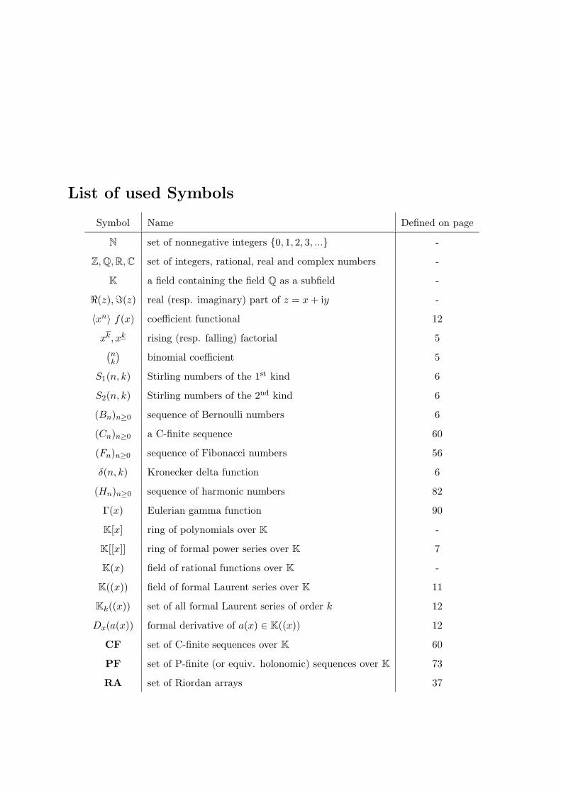
List of used Symbols
Symbol Name Defined on page
N set of nonnegative integers {0, 1, 2, 3, ...} -
Z,Q,R,C set of integers, rational, real and complex numbers -
K a field containing the field Q as a subfield -
ℜ(z),ℑ(z) real (resp. imaginary) part of z = x+ iy -
⟨xn⟩ f(x) coefficient functional 12
xk, xk rising (resp. falling) factorial 5(nk
)binomial coefficient 5
S1(n, k) Stirling numbers of the 1st kind 6
S2(n, k) Stirling numbers of the 2nd kind 6
(Bn)n≥0 sequence of Bernoulli numbers 6
(Cn)n≥0 a C-finite sequence 60
(Fn)n≥0 sequence of Fibonacci numbers 56
δ(n, k) Kronecker delta function 6
(Hn)n≥0 sequence of harmonic numbers 82
Γ(x) Eulerian gamma function 90
K[x] ring of polynomials over K -
K[[x]] ring of formal power series over K 7
K(x) field of rational functions over K -
K((x)) field of formal Laurent series over K 11
Kk((x)) set of all formal Laurent series of order k 12
Dx(a(x)) formal derivative of a(x) ∈ K((x)) 12
CF set of C-finite sequences over K 60
PF set of P-finite (or equiv. holonomic) sequences over K 73
RA set of Riordan arrays 37
Contents
1 Introduction 11.1 Overview . . . . . . . . . . . . . . . . . . . . . . . . . . . . . . . . . . . . . 11.2 Software packages we used . . . . . . . . . . . . . . . . . . . . . . . . . . . 21.3 How to read the thesis . . . . . . . . . . . . . . . . . . . . . . . . . . . . . 31.4 Acknowledgements . . . . . . . . . . . . . . . . . . . . . . . . . . . . . . . 4
2 Preliminaries 52.1 Combinatorial notions . . . . . . . . . . . . . . . . . . . . . . . . . . . . . 52.2 Manipulation of power series . . . . . . . . . . . . . . . . . . . . . . . . . . 7
2.2.1 Operations on formal power series . . . . . . . . . . . . . . . . . . . 72.2.2 Formal Laurent series . . . . . . . . . . . . . . . . . . . . . . . . . . 112.2.3 Differentiation and integration . . . . . . . . . . . . . . . . . . . . . 122.2.4 The concept of res . . . . . . . . . . . . . . . . . . . . . . . . . . . 18
2.3 Rules for the res-functional . . . . . . . . . . . . . . . . . . . . . . . . . . 232.4 Connection to complex analysis . . . . . . . . . . . . . . . . . . . . . . . . 26
3 The Riordan group 323.1 The Riordan array approach . . . . . . . . . . . . . . . . . . . . . . . . . . 323.2 Characterization of Riordan arrays . . . . . . . . . . . . . . . . . . . . . . 37
4 Application to Symbolic Summation 434.1 The Identities of Abel and Gould . . . . . . . . . . . . . . . . . . . . . . . 43
4.1.1 Applying the Egorychev Method . . . . . . . . . . . . . . . . . . . 464.1.2 Applying the Riordan Array paradigm . . . . . . . . . . . . . . . . 48
4.2 Multi-Sum Identities . . . . . . . . . . . . . . . . . . . . . . . . . . . . . . 504.3 Another Mathematical Monthly Problem . . . . . . . . . . . . . . . . . . . 534.4 Symbolic Sums involving C-finite sequences . . . . . . . . . . . . . . . . . 554.5 An explicit formula for Stirling numbers . . . . . . . . . . . . . . . . . . . 654.6 Further non-hypergeometric examples . . . . . . . . . . . . . . . . . . . . . 67
i
4.7 Symbolic Sums involving holonomic sequences . . . . . . . . . . . . . . . . 714.8 Symbolic Sums involving trigonometric functions . . . . . . . . . . . . . . 75
4.8.1 Applying the Egorychev Method . . . . . . . . . . . . . . . . . . . 764.8.2 Applying the Riordan Array paradigm . . . . . . . . . . . . . . . . 77
4.9 An Identity for Jacobi polynomials P(α,β)n (x) . . . . . . . . . . . . . . . . . 78
4.10 An Example with Harmonic Numbers . . . . . . . . . . . . . . . . . . . . . 824.10.1 Solution by the Sigma package . . . . . . . . . . . . . . . . . . . . . 824.10.2 A Guessing try . . . . . . . . . . . . . . . . . . . . . . . . . . . . . 834.10.3 Applying the Egorychev method . . . . . . . . . . . . . . . . . . . . 854.10.4 Solution by the HolonomicFunctions package . . . . . . . . . . . . . 874.10.5 Application of change of variables . . . . . . . . . . . . . . . . . . . 88
4.11 Analytic aspects . . . . . . . . . . . . . . . . . . . . . . . . . . . . . . . . . 89
Chapter 1
Introduction
1.1 Overview
This master thesis contributes to problem solving methods related to symbolic summa-tion and generating functions of combinatorial sequences. During the last years severalcreative and effective approaches towards systematic treatments have been introduced.The Egorychev method is one such attempt.
One of the reasons why the Egorychev method is that powerful is that it takes advantageof the Lagrange inversion rule in a constructive way to derive a closed form for a gener-ating function. With this application one can prove complicated identities such as Abel’sidentity
n∑k=0
(n
k
)a(a+ k)k−1(b+ n− k)n−k = (a+ b+ n)n (1.1)
or Gould’s identity
r∑k=0
r
r − kq
(r − qk
k
)(p+ kq
n− k
)=
(p+ r
n
). (1.2)
A somewhat similar approach is the concept of the Riordan group that also applies theLagrange inversion rule for proving combinatorial identities. Clever construction of Rior-dan arrays makes it easy to discover identities of similar type.
One of the reasons for this thesis was the interest of the author to compute sums that arenot applicable to classical algorithms. The author has attended the Algorithmic Combi-natorics Seminar of the RISC combinatorics group for several years and got an impression
1
of the power of symbolic summation techniques and its utilization in several applications.In particular, the author wants to mention the work of Dr. Kauers, Dr. Schneider, Dr.Koutschan and the advisor of this thesis, Prof. Paule. The author wants to thank themfor their enthusiasm and their always present will to give insights in their work and dis-cussing until all details were understood. We will describe some of their work in thefollowing chapters and also take a look on how their developments can be applied to solvesymbolic summation problems.
This thesis focusses on combinatorial numbers such as Stirling numbers, Bernoulli num-bers and binomial coefficients. Combinatorial numbers express some of the most funda-mental properties of combinatorial objects in mathematics (as for instance the numberof subsets with certain properties, ...) and are in fact not that trivial to handle. A goalof this master thesis is to present some approaches that can be used to derive closedform solutions for combinatorial sums. Also several concrete examples are given to seeimmediately how the machinery developed by Egorychev and Shapiro/Sprugnoli provesidentities arising (among others) in combinatorial mathematics.
One might speculate that there is a way to automatize the Lagrange inversion rule on acomputer algebra system which would lead to a new algorithmic method that assists infinding closed forms for combinatorial sums. Especially the inversion rule which boils theproblem down to pattern matching has the potential to be implemented on some computeralgebra system. Unfortunately this is only part of the work as we will see, because weneed some preprocessing steps which is not that easy to automatize. Therefore we stillneed to go back to paper and pencil for particular problem classes.
1.2 Software packages we used
In this work the author used several software packages (most of them developed by theAlgorithmic Combinatorics group of RISC Linz) for the Mathematica computer algebrasystem. We demonstrate how this packages can be used to solve symbolic summationproblems. The following packages have been used in this thesis (in alphabetical order)
• M. Kauers: Stirling [Kau07]: a Mathematica package for computing recurrenceequations of sums involving Stirling numbers or Eulerian numbers.
• C. Koutschan: Holonomic Functions [Kou09, Kou10]: a Mathematica package fordealing with multivariate holonomic functions, including closure properties, sum-mation, and integration.
2
• C. Mallinger: Generating Functions [Mal96]: a Mathematica package for manipula-tions of univariate holonomic functions and sequences.
• P. Paule, M. Schorn [PS95]: the Paule/Schorn implementation of Gosper’s andZeilberger’s algorithm in Mathematica.
• M. Petkovsek: Hyper [Pet98]: a Mathematica implementation of Petkovsek’s algo-rithm Hyper.
• C. Schneider: Sigma [Sch01, Sch04, Sch07]: a Mathematica package for discoveringand proving multi-sum identities.
The packages developed at RISC can be obtained from
http://www.risc.jku.at/research/combinat/software/
1.3 How to read the thesis
The thesis is divided into four chapters, which depend upon each other. In the followingchapter 2 we clarify the notion of combinatorial numbers and recall their combinatorialinterpretation. Further we go into details how to operate on formal power series andLaurent series. The central element in this thesis is the notion of residue functional. Adetailed account will be devoted to its application on Laurent series. Finally we willinvestigate how this is related to the concept of residue appearing in complex analysis.Chapter 3 is devoted to the notion of Riordan arrays that closely relates to manipulatingpower series on coefficient level. We examine ways of characterizing Riordan arrays byits A- and Z-sequence. At the end of the day we want to apply the developed machineryto solve problems in the area of symbolic summation and computing closed forms forgenerating functions. This will be the main focus in chapter 4. This chapter will alsoprovide some new aspects (to the author’s opinion). We apply Egorychev’s approach, toGould’s identity (1.2) and to a generalization of Abel’s identity (4.12) that is based onRiordan arrays. The power of the Egorychev method on multi-sum identities is demon-strated on an American Mathematical Monthly problem (see section 4.2) that has beenworked out (with input provided by the BSI Problems group, Bonn). An application ofMathematica packages is discussed to solve this kind of problems. As the name suggests,the next section 4.3 shows a recent American Mathematical Monthly problem that wassolved by deriving a residue representation and evaluating it explicitly in closed form.During the examination of a symbolic sum involving Fibonacci numbers the author could
3
generalize the shape of the summand to evaluate sums with binomial coefficients andC-finite sequences. This generalization (Thm. 4.4.5) includes an exercise of [Wil06, Ex.4.16] as special case. Next we will show how to derive a residue representation for anexplicit formula for Stirling numbers of the second kind (4.34) (that reflects the gener-ating function). Stirling numbers are also subject in the identities (4.36), (4.37) thatare out of scope for the known methods introduced in [PWZ96]. For proving an identity(equality of two binomial sums) that is needed for computing the generating function ofJacobi polynomials we will make use of the method of coefficients although Zeilberger’salgorithm as well as the Snake Oil method would also be applicable. Finally we give asummation example involving harmonic numbers and present several ways to compute itin closed form. The final subsection is a remark on asymptotic analysis.
1.4 Acknowledgements
I joined the combinatorics group at RISC in spring 2008. Since that time I had thehonor of learning from experts at this group both in theoretical lectures and practicalresearch. My first thank undoubtedly goes to the leader of this group and the advisorof this thesis, Prof. Peter Paule. With his enthusiasm and his advices he handled tomotivate me in writing this thesis. He also introduced the classic tools in his lectures andshowed where still further research could be done. The author was financially supportedby the Doctoral Program Computational Mathematics (W1214) whom I want to thanktoo. Further I want to thank Dr. Schneider for introducing me to his Sigma package,Dr. Koutschan for demonstrating his HolonomicFunctions package and Dr. Kauers forhis inauguration on his Stirling package (and challenging exercises from his side that arepart of this thesis). Dr. Kauers also was so kind to provide a LATEX package for fancytypesetting of Mathematica source code listings. I want to express my acknowledgementsto the faculty of RISC for teaching me that much in symbolic algorithms. They nevergot tired of answering my questions. Also among the PhD students I want to say thankyou for helpful scientific (and non-scientific) discussions, especially to my friends JakobAblinger, Silviu Radu and Clemens Raab. Finally I must not forget to thank my family,who made all this possible.
4
Chapter 2
Preliminaries
2.1 Combinatorial notions
In chapter 6 of the book [GKP94] there is a comprehensive repertoire on combinatorialnumbers. As mentioned in the introduction we will have a look at some of them tosummarize the most important ones.
Definition 2.1.1 (Rising/falling factorials)Let R be an arbitrary ring with unity, x ∈ R, k ∈ N. We define the rising (resp. falling)factorial by (see [GKP94, p.47/48])
xk = x(x+ 1) . . . (x+ k − 1), k ≥ 1, (2.1)
xk = x(x− 1) . . . (x− k + 1), k ≥ 1, (2.2)
x0 = x0 = 1. (2.3)
Definition 2.1.2 (Binomial coefficients)Let R be a commutative ring containing Q and let λ ∈ R and k ∈ Z. Then(
λ
k
):=
λk
k!=
λ(λ− 1) . . . (λ− k + 1)
k(k − 1) . . . 1, k ≥ 0, (2.4)(
λ
k
):= 0, k < 0. (2.5)
For the case that n, k ∈ N we have the formula:(n
k
)=
n!
k!(n− k)!=
(n
n− k
), (2.6)
and the usual convention that(nk
)= 0 when k > n.
5
Theorem 2.1.1 (Binomial theorem, [KP11], p. 87-89)The binomial theorem states that for n ∈ N and any a, b ∈ K we have
(a+ b)n =n∑
k=0
(n
k
)akbn−k. (2.7)
As we have seen in Def. 2.1.2 it is also useful to consider the cases where n ∈ −N. Inthis case we have for n ∈ N, a, b ∈ K:
(a+ b)−n =∞∑k=0
(−n
k
)akb−n−k =
∞∑k=0
(−n)k
k!akb−n−k. (2.8)
Definition 2.1.3 (Stirling numbers of the 1st kind)Let n, k ∈ N. The signless Stirling numbers of the 1st kind count the number of permuta-tions of n objects with exactly k cycles. We will denote them by
S1(n, k). (2.9)
Definition 2.1.4 (Stirling numbers of the 2nd kind)Let n, k ∈ N. The symbol
S2(n, k) (2.10)
stands for the number of ways to partition a set of n objects into k nonempty subsets.
Definition 2.1.5 (Bernoulli numbers)Let n ∈ N. The sequence of Bernoulli numbers (see [FB07, p.114, Ex. 3])
(Bn)n≥0 (2.11)
is recursively defined by
B0 = 1,n∑
k=0
(n+ 1
k
)Bk = 0, n ≥ 1.
Definition 2.1.6 (The Kronecker symbol)The Kronecker Symbol is given by
δ(n, k) =
{1, n = k,
0, n = k.(2.12)
6
2.2 Manipulation of power series
In this section we summarize the most basic facts concerning power series. For a detailedtreatment see [GCL92, Wil06, GKP94, KP11].
For any commutative ring R containing Q as a subring, the notation R[[x]] denotes theset of all expressions of the form
A(x) ∈ R[[x]] : A(x) =∞∑k=0
akxk, ak ∈ R. (2.13)
In other words R[[x]] denotes the set of all formal power series in the indeterminate x overthe ring R. We call A(x) =
∑∞k=0 akx
k the (ordinary) generating function associated tothe sequence (ak)k≥0.The order ord(A(x)) of a nonzero power series A(x) is the least integer k such that ak = 0.The exceptional case where ak = 0 for all k is called the zero power series. It is commonto define the order of the zero power series to be infinity. For a nonzero power seriesA(x) =
∑∞k=0 akx
k ∈ R[[x]] with ord(A(x)) = l the term alxl is called the low order term
of A(x), al is called the low order coefficient, and a0, also written A(0), is called theconstant term.
2.2.1 Operations on formal power series
It is usual to define the binary operations of addition and multiplication in the set R[[x]]as follows. If
a(x) =∞∑k=0
akxk and b(x) =
∞∑k=0
bkxk,
then the power series addition is defined by
c(x) = a(x) + b(x) =∞∑k=0
ckxk,
whereck = ak + bk, k ≥ 0.
Power series multiplication is defined by
d(x) = a(x) · b(x) =∞∑k=0
dkxk,
7
wheredk = a0bk + · · ·+ akb0, k ≥ 0.
If K a field, (K[[x]],+, ·) forms a commutative ring with unity 1 = 1 + 0 · x+ 0 · x2 + ....
Lemma 2.2.1 (K[[x]],+, ·) is an integral domain.
Lemma 2.2.2 (K[[x]],+, ·) is a principal ideal domain.
Lemma 2.2.3Let R be any commutative ring containing Q as a subring. The units (invertible elements)in R[[x]] are all power series A(x) whose constant terms A(0) are units in the coefficientdomain R.
Proof. If a(x) =∑∞
k=0 akxk is a unit in R[[x]] then there must exist a power series b(x) =∑∞
k=0 bkxk such that a(x)b(x) = 1. By the definitions of power series multiplication we
must have
1 = a0b0,
0 = a0b1 + a1b0,...
0 = a0bn + a1bn−1 + · · ·+ anb0, etc.
Thus, a0 is a unit in R with a−10 = b0. Conversely, if a0 is a unit in R then the above
equation can be solved for the bk as follows:
b0 = a−10 ,
b1 = −a−10 (a1b0),
...
bn = −a−10 (a1bn−1 + · · ·+ anb0), etc.
This way, we construct b(x) such that a(x)b(x) = 1, so a(x) is a unit in R[[x]]. 2
Lemma 2.2.4 If the coefficient domain R (an arbitrary ring with unity) is an integraldomain then R[[x]] is also an integral domain.
Proof. We have to show that for given a(x), b(x) ∈ R[[x]] such that
a(x) =∞∑k=0
akxk = 0, b(x) =
∞∑k=0
bkxk = 0,
8
where for k ∈ N: ak, bk ∈ R, we have that their product a(x)b(x) is not equal to zero.Because a(x) = 0 there exist ai = 0 for some i ∈ N and similar j ∈ N such that bj = 0.Let i, j be minimal with this property. The product a(x)b(x) is given by
c(x) :=∞∑n=0
cnxn = a(x)b(x),
where
cn =n∑
k=0
akbn−k, n ≥ 0.
By assumption ak = 0 for k < i and bn−k = 0 for n− k < j or k > n− j. Therefore, forn = i+ j we find
ci+j =
i+j∑k=0
akbi+j−k = aibj.
The coefficient domain R is by assumption an integral domain and therefore free of zerodivisors. ai and bj are nonzero, so ci+j is nonzero. Therefore c(x) = 0. 2
Theorem and Definition 2.2.1 (General binomial theorem, [KP11], p.89)For λ ∈ R, (R a commutative ring containing Q as a subring) the expression (1 + x)λ
does not have a meaning as formal power series. We still have
(1 + x)λ =∞∑n=0
(λ
n
)xn, x ∈ K, |x| < 1, (2.14)
as analytic power series. Therefore it is reasonable to take
(1 + x)λ :=∞∑n=0
(λ
n
)xn ∈ R[[x]] (2.15)
as the definition of the symbol (1 + x)λ. With this definition, we can prove, the multipli-cation law
(1 + x)λ(1 + x)µ = (1 + x)λ+µ (2.16)
in R[[x]]. By applying the definition of product in R[[x]] this is equivalent to the identity
n∑k=0
(λ
k
)(µ
n− k
)=
(λ+ µ
n
)n ≥ 0, λ, µ ∈ R, (2.17)
that is known as Vandermonde convolution ([GKP94, p. 170, (5.27)]).
9
Now we consider the notion of limit in K[[x]]. With this we can define composition offormal power series.
Definition 2.2.1 ([KP11], p.24)A sequence (ak(x))k≥0 of formal power series in K[[x]] converges to another formal powerseries a(x) ∈ K[[x]] if the ak(x) get arbitrarily close to a(x). Formally, (ak(x))k≥0 con-verges to a(x) in K[[x]] if and only if
limk→∞
ord(a(x)− ak(x)) = ∞,
i.e., if and only if
∀n ∈ N ∃k0 ∈ N ∀k ≥ k0 : ord(a(x)− ak(x)) > n.
Definition 2.2.2 (Composition of power series)Let a(x) =
∑∞n=0 anx
n, b(x) ∈ K[[x]] be such that ord(b(x)) ≥ 1. Consider the sequence(ck(x))k≥0 defined by
ck(x) =k∑
j=0
ajb(x)j.
The composition of a(x) and b(x) is defined by
a(b(x)) :=∞∑n=0
anb(x)n := lim
k→∞ck(x) = c(x). (2.18)
The composition of power series is compatible with addition and multiplication as thefollowing theorem shows.
Theorem 2.2.1 ([KP11], p.26)For every fixed u(x) ∈ K[[x]] with ord(u(x)) ≥ 1 the map
Φu : K[[x]] −→ K[[x]],
a(x) 7−→ a(u(x)),
is a ring homomorphism.
Proof. See [KP11, p. 26, Thm. 2.6] 2
Note that 1x
/∈ K[[x]] but lies in its quotient field, i.e. 1x∈ K((x)), the field of formal
Laurent series.
10
2.2.2 Formal Laurent series
By Lemma 2.2.1 K[[x]] is an integral domain. So one can construct the quotient field:
K((x)) =
{a(x)
b(x): a(x), b(x) ∈ K[[x]] ∧ b(x) = 0
}.
We call this construction the field of formal Laurent series over K.
Lemma 2.2.5K((x)) =
{xkc(x) : k ∈ Z, c(x) ∈ K[[x]]
}.
Proof. For one inclusion take f(x) ∈ K((x)). Hence f(x) = a(x)b(x)
for some a(x), b(x) ∈K[[x]] and b(x) = 0. If we extract xi such that
a(x) =∞∑n=0
anxn = xi
∞∑n=0
αnxn
︸ ︷︷ ︸=:α(x)
,
with α0 = 0 and do the same for
b(x) =∞∑n=0
bnxn = xj
∞∑n=0
βnxn
︸ ︷︷ ︸=:β(x)
,
with β0 = 0,we find by Lemma 2.2.3 a multiplicative inverse of β(x). Hence the expression
a(x)
b(x)=
xiα(x)
xjβ(x)= xi−j α(x)
β(x)︸ ︷︷ ︸∈K[[x]]
is well defined and of the desired form.
For the other direction take f(x) ∈{xkc(x) : k ∈ Z, c(x) ∈ K[[x]]
}: by definition f(x) =
xkc(x) for some k ∈ Z, c(x) ∈ K[[x]]. If k ∈ N0 we have:
xkc(x) = xk
∞∑n=0
cnxn =
∞∑n=0
cnxn+k =
∞∑n=k
cn−kxn,
and by setting a(x) =∑∞
n=k cn−kxn and b(x) = 1 = 1 + 0 · x + 0 · x2 + ... we have
xkc(x) = a(x)b(x)
∈ K((x)).
For k ∈ −N we get the desired form by setting a(x) = c(x) and b(x) =∑∞
n=0 bnxn = x−k,
i.e. (bn)n≥0 : (δ(−k, n))n≥0. 2
11
This Lemma gives the justification to view a formal Laurent series as follows
K((x)) =
{∞∑
n=−∞
anxn an ∈ K ∧ finitely many an = 0 where n < 0
}.
Notation: For k ∈ Z:
Kk((x)) := { f ∈ K((x)) | ord(f(x)) = k} ⊂ K((x)). (2.19)
Definition 2.2.3 (Coefficient functional)Let
f(x) =∑k∈Z
fkxk ∈ K((x)).
We will frequently use the notation
⟨xn⟩ f(x) := fn, n ∈ Z.
We definef(0) := ⟨x0⟩ f(x) = f0.
An elementary property of this functional is given by
⟨xn⟩ xkf(x) = ⟨xn−k⟩f(x), n, k ∈ Z.
In subsection 2.2.4 we will give ⟨x−1⟩ f(x) a special name.
2.2.3 Differentiation and integration
If R is a commutative ring (resp. a field) and D : R → R is such that
D(a+ b) = D(a) +D(b), (2.20)
D(a · b) = D(a)b+ aD(b) (2.21)
for all a, b ∈ R, then D is called a (formal) derivation on R and the pair (R,D) is called adifferential ring (resp. a differential field). Next we define the formal derivative on K((x)).
Definition 2.2.4 (Formal derivative)Let, for k0 ∈ Z,
a(x) = x−k0
∞∑k=0
akxk ∈ K((x)).
12
A derivation on the field of formal Laurent series is given by
Dx : K((x)) −→ K((x)),
a(x) = x−k0
∞∑k=0
akxk 7−→ Dx(a(x)) := −k0x
−k0−1
∞∑k=0
akxk + x−k0
∞∑k=0
ak+1(k + 1)xk.
Notation: For f(x) ∈ K((x)) we also write:
f ′(x) := Dx(f(x)),
f ′′(x) := D2x(f(x)) := Dx(Dx(f(x))),
f (k)(x) := Dkx(f(x)) := Dx(. . . Dx︸ ︷︷ ︸
k times
(f(x)) . . . ), etc.
Note that this definition contains the ring of formal power series as special case by settingk0 = 0, i.e. f(x) =
∑∞k=0 akx
k and
Dx(f(x)) = Dx
(∞∑k=0
akxk
)=
∞∑k=1
akkxk−1 =
∞∑k=0
ak+1(k + 1)xk. (2.22)
We will not distinguish the symbol Dx for K((x)) resp. K[[x]].
Lemma 2.2.6 (K[[x]], Dx) is a differential ring.
Lemma 2.2.7 (K((x)), Dx) is a differential field.
Lemma 2.2.8Let f(x), (fn(x))n≥0 be in K((x)) such that limn→∞ ord(fn(x)) = ∞ and
f(x) =∞∑n=0
fn(x)
Then:
• For k ∈ Z
⟨xk⟩ f(x) =∞∑n=0
⟨xk⟩ fn(x)
•
Dx(f(x)) =∞∑n=0
Dx(fn(x))
13
Proof. By definition of the infinite sum we have that
⟨xk⟩ f(x) = ⟨xk⟩∞∑n=0
fn(x) = ⟨xk⟩ limN→∞
N∑n=0
fn(x)
Now, because of our assumption that limn→∞ ord(fn(x)) = ∞, we know that there existsan index M such that for all m ≥ M we have that ord(fm(x)) > k. Hence we can splitthe sum.
= ⟨xk⟩ limN→∞
(M∑n=0
fn(x) +N∑
n=M+1
fn(x)
)
= ⟨xk⟩M∑n=0
fn(x) + ⟨xk⟩ limN→∞
N∑n=M+1
fn(x)
We have chosen M such that ∀i ∈ N: ord(fM+i(x)) > k, hence the second sum does notcontribute to ⟨xk⟩. Now we use a linearity argument, i.e.,
⟨xk⟩M∑n=0
fn(x) =M∑n=0
⟨xk⟩fn(x),
which proves the theorem, by our choice of M . For the second statement, we plug in thedefinition of the infinite sum:
Dx(f(x)) = Dx
(∞∑n=0
fn(x)
)= Dx
(lim
N→∞
N∑n=0
fn(x)
)Now, because limn→∞ ord(fn(x)) = ∞ we know that for all K ∈ N there exists M ∈ Nsuch that for all m ≥ M : ord(fm(x)− f(x)) > K. Hence, we find that
Dx
(lim
N→∞
N∑n=0
fn(x)
)= Dx
(lim
N→∞
(M∑n=0
fn(x) +N∑
n=M+1
fn(x)
))
= Dx
(M∑n=0
fn(x)
)+Dx
(lim
N→∞
(N∑
n=M+1
fn(x)
))
By our choice of M , we know that the second sum is of the form
N∑n=M+1
fn(x) = xK+1g(x), g(x) ∈ K[[x]].
14
If we differentiate this expression we get
Dx(xK+1g(x)) = (K + 1)xKg(x) + xK+1Dx(g(x)) −→ 0.
as K tends to infinity. Again the linearity property of the Dx operator,
Dx
(M∑n=0
fn(x)
)=
M∑n=0
Dx (fn(x)) ,
proves our claim. 2
Proposition 2.2.1 The following rules hold for f(x), g(x) ∈ K((x)), n ∈ N:
•Dx
(f(x)
g(x)
)=
Dx(f(x))g(x)− f(x)Dx(g(x))
g(x)2, g(x) = 0, (2.23)
•Dx (f(x)
n) = n · f(x)n−1Dx(f(x)), (2.24)
• If f(x) ∈ K0((x)), ord(g(x)) ≥ 1:
Dx (f(g(x))) = Dt(f(t))|t=g(x)Dx(g(x))
= f ′(g(x))g′(x)(2.25)
Proof. For the first statement we show that Dx(1) = 0. Indeed,
Dx(1) = Dx(1 · 1) = 1 ·Dx(1) + 1 ·Dx(1) = Dx(1) +Dx(1) ⇒ Dx(1) = 0.
From this we find that:
0 = Dx(1) = Dx
(g(x)
g(x)
)= g(x)Dx
(1
g(x)
)+
1
g(x)Dx(g(x))
⇒ Dx
(1
g(x)
)= − 1
g(x)2Dx(g(x))
Now we can apply the product rule (2.21):
Dx
(f(x)
g(x)
)= f(x)Dx
(1
g(x)
)+
1
g(x)Dx(f(x))
= f(x)
(−Dx(g(x))
g(x)2
)+
1
g(x)Dx(f(x))
=Dx(f(x))g(x)− f(x)Dx(g(x))
g(x)2.
15

For the second statement we apply induction on n. The base cases n = 0, 1 are trivialfrom the definition. Now let us suppose that for fixed n we have that
Dx(f(x)n) = nf(x)n−1Dx(f(x))
We consider now
Dx(f(x)n+1) = Dx(f(x)
nf(x)) = f(x)nDx(f(x)) + f(x)Dx(f(x)n)
= f(x)nDx(f(x)) + nf(x)nDx(f(x))
= (n+ 1)f(x)nDx(f(x)),
which proves the statement.
For the third statement let f(x) =∑∞
k=0 fkxk. By Lemma 2.2.8 we can exchange sum-
mation and limit. From this we find that
Dx(f(g(x)) = Dx
(∞∑k=0
fkg(x)k
)= Dx
(limn→∞
n∑k=0
fkg(x)k
)
= limn→∞
n∑k=0
Dx(fkg(x)k) = lim
n→∞
n∑k=0
fkDx(g(x)k)
= limn→∞
n∑k=1
fkkg(x)k−1Dx(g(x)) = Dx(g(x)) lim
n→∞
n∑k=1
fkkg(x)k−1
= Dt(f(t))|t=g(x)Dx(g(x)) = g′(x)f ′(g(x)),
that proves the chain-rule. 2
Example 2.2.1 The exponential ex is a shortcut notation for the formal power series
eαx := exp(αx) :=∞∑k=0
αk
k!xk ∈ K[[x]], α ∈ K.
It’s formal derivative is given by
Dx(eαx) = Dx
(∞∑k=0
αk
k!xk
)=
∞∑k=0
αk+1
(k + 1)!(k + 1)xk = α
∞∑k=0
αk
k!xk = αeαx. (2.26)
This power series satisfies:
eαx · eβx =
(∞∑k=0
αk
k!xk
)(∞∑k=0
βk
k!xk
)=
∞∑n=0
xn
n!
(n∑
k=0
(n
k
)αkβn−k
)(2.7)=
∞∑n=0
(α+ β)n
n!xn = e(α+β)x, α, β ∈ K.
(2.27)
16
Similar relations hold for (1 + x)λ ∈ R[[x]] (R a commutative ring containing Q as asubring). We do not carry out the proof in detail, but state the identity for sake ofcompleteness (as we will need it in chapter 4):
Dx((1 + x)λ) = Dx
(∞∑k=0
(λ
k
)xk
)= λ · (1 + x)λ−1. (2.28)
Definition 2.2.5 (Formal integral)The formal integral of the formal power series
f(x) =∞∑k=0
akxk ∈ K[[x]]
is defined by∫x
: K[[x]] −→ K[[x]],
f(x) =∞∑k=0
akxk 7−→
∫x
f(x) =
∫x
∞∑k=0
akxk :=
∞∑k=0
akk + 1
xk+1 =∞∑k=1
ak−1
kxk.
Proposition 2.2.2 ([KP11], p.20, Thm. 2.3)For all a(x) ∈ K[[x]]:
•Dx
(∫x
a(x)
)= a(x), (2.29)
• ∫x
Dxa(x) = a(x)− a(0), (2.30)
•⟨xn⟩ a(x) = 1
n!(Dn
x(a(x))|x=0. (2.31)
Proof. Throughout the proof, let a(x) =∑∞
k=0 akxk ∈ K[[x]]. The first statement is
obtained as follows:
Dx
(∫x
a(x)
)= Dx
(∫x
∞∑k=0
akxk
)= Dx
(∞∑k=1
ak−1
kxk
)
=∞∑k=0
akk + 1
(k + 1)xk =∞∑k=0
akxk = a(x).
17
For the second statement we calculate∫x
Dx(a(x)) =
∫x
Dx
(∞∑k=0
akxk
)=
∫x
∞∑k=0
ak+1(k + 1)xk
=∞∑k=0
ak+1
k + 1(k + 1)xk+1 =
∞∑k=0
ak+1xk+1
=∞∑k=1
akxk = a(x)− a(0).
To prove (2.31) we proceed by induction on n. The base case n = 0 is easily checked:
⟨x0⟩a(x) = a0 =1
0!a(0).
Now suppose for some fixed n ∈ N we have that:
⟨xn⟩ a(x) = 1
n!Dn
x(a(x))|x=0
The connection to the coefficient of xn+1 is given by the derivative as follows
⟨xn+1⟩ a(x) = ⟨xn⟩ Dx(a(x)) ·1
n+ 1
=1
n!Dn
x (Dx(a(x))) |x=01
n+ 1
=1
(n+ 1)!Dn+1
x (a(x))|x=0.
2
2.2.4 The concept of res
Definition 2.2.6 (res-functional)If
C(x) =∞∑
k=−∞
ckxk ∈ K((x)),
then we define the formal residue res of C(x) to be the coefficient of x−1, i.e.,
resx
C(x) := ⟨x−1⟩ C(x) = c−1.
18
Remark: resx
A(x) is a purely formal operation; more precisely, a linear functional on
the K-vector space K((x)). We will set this later into a context to the analytic meaningin complex analysis, but whenever we talk of application of the res-operator we meanextraction of the coefficient of x−1.
Lemma 2.2.9 (Coefficient formula)If
A(x) =∞∑k=0
akxk ∈ K[[x]]
is the generating function for the sequence (ak)k≥0 it follows that
ak = ⟨xk⟩A(x) = resx
A(x)x−k−1, k ≥ 0.
Lemma 2.2.10 For all A(x) ∈ K((x)): resx
Dx(A(x)) = 0
Proof. If we consider
A(x) = a−n0x−n0 + ...+ a−1x
−1 + a0 + a1x+ a2x2 + ...
thenDx(A(x)) = −n0a−n0x
−n0−1 + ...+ (−1)a−1x−2 + 0 + a1 + 2a2x+ ...
and hence ⟨x−1⟩Dx(A(x)) = 0. 2
Lemma 2.2.11 ([Ros97], p. 41, Lemma 48)Let g(x) ∈ K1((x)), n ∈ Z. Then:
resx
Dx(g(x))
g(x)n+1= δ(n, 0).
Proof. For n = 0 we have
Dx(g(x))g(x)−n−1 = − 1
nDx(g(x)
−n),
which has residue zero by Lemma 2.2.10.
For n = 0, we write g(x) = x/h(x) where h(x) =∑∞
k=0 hkxk ∈ K[[x]] such that h0 = 0.
By Lemma 2.2.3 such a representation of g(x) exists. With this substitution, we have
Dx(g(x))
g(x)=
1
g(x)
(Dx
(x
h(x)
))=
h(x)
x
(h(x)− xDx(h(x))
h(x)2
)=
1
x− Dx(h(x))
h(x).
19
1/h(x) is a well defined power series of order 0, the power series Dx(h(x)) has order ≥ 0,so the product Dx(h(x))
1h(x)
has order ord(Dx(h(x)))+ord(1/h(x)) ≥ 0. Therefore
resx
Dx(g(x))
g(x)= res
x
(1
x− Dx(h(x))
h(x)
)= res
x
(1
x
)+ res
x
(Dx(h(x))
h(x)
)= 1.
2
For computing with formal Laurent series we need the following important theorem
Theorem 2.2.2 (Lagrange, [Ros97], p. 38, Thm. 42)Let f(x), g(x) ∈ K[[x]] formal power series with ord(g(x)) = 1 and let (an)n≥0 ∈ KN besuch that
f(x) =∞∑n=0
ang(x)n. (2.32)
Then we have that
a0 = ⟨x0⟩ f(x), (2.33)
am = resx
f(x)Dx(g(x))g(x)−m−1, m ≥ 1. (2.34)
Proof. Several different proofs are given in [Ros97]. One of them goes like this:
The first statement on a0 is immediate since g(x) does not contribute. Hence, we havethat
f(0) = ⟨x0⟩f(x) = a0.
The statement on general am essentially relies on Lemma 2.2.11. If we multiply both sidesof (2.32) by Dx(g(x))g(x)
−m−1 (for m ∈ N,m ≥ 1) we get by Lemma 2.2.8:
f(x)Dx(g(x))g(x)−m−1 =
∞∑n=0
anDx(g(x))
g(x)m−n+1. (2.35)
If we now apply the res-functional we find by Lemma 2.2.11 and Lemma 2.2.8 that
resx
f(x)Dx(g(x))g(x)−n−1 = res
x
∞∑n=0
anDx(g(x))
g(x)m−n+1
=∞∑n=0
an resx
Dx(g(x))
g(x)m−n+1
=∞∑n=0
anδ(n,m) = am.
2
20
In concrete examples (see section 4.1.2) we will find it useful, as in the proof of Lemma2.2.11, to consider a power series of order 1 as a quotient of two power series as follows:
g(x) :=x
h(x), (2.36)
where h(x) ∈ K0((x)). If we apply Thm. 2.2.2 to this choice, use the chain-rule in K[[x]](see Proposition 2.2.2) and multiply both sides of (2.32) by g(x)−m, we find by Lemma2.2.8 that:
Dx(f(x)) =∞∑n=1
anng(x)n−1Dx(g(x)),
Dx(f(x))
g(x)m=
∞∑n=1
annDx(g(x))
g(x)m−n+1.
Now we apply on both sides the res-functional together with Lemma 2.2.8 and Lemma2.2.11:
resx
Dx(f(x))g(x)−m =
∞∑n=1
ann resx
Dx(g(x))
g(x)m−n+1
=∞∑n=1
annδ(m,n)
= m · am.
If we finally expand g(x) according to (2.36) we get that:
m · am = resx
Dx(f(x))g(x)−m
= ⟨x−1⟩ Dx(f(x))h(x)mx−m
= ⟨xm−1⟩ Dx(f(x))h(x)m.
Corollary 2.2.1Under the assumptions (and with the notions) of Thm. 2.2.2 where h(x) ∈ K0((x)) and
g(x) =x
h(x),
we have for m ≥ 1:
am = resx
f(x)Dx(g(x))g(x)−m−1 =
1
m⟨xm−1⟩Dx(f(x))h(x)
m. (2.37)
21
Remark: An alternative derivation of Cor. 2.2.1 from Thm. 2.2.2 is straight-forwardfrom the identity
0 = ⟨x−1⟩ 1mDx
(f(x)g(x)−m
), m ≥ 1. (2.38)
Theorem 2.2.3 (Implicit function theorem, [KP11], Thm. 2.9, p. 33)Let a(x, y) ∈ K[[x, y]] be such that
a(0, 0) = 0 and (Dya)(0, 0) = 0. (2.39)
Then there exists a unique formal power series f(x) ∈ K[[x]] with f(0) = 0 such thata(x, f(x)) = 0.
Proof. See [KP11, p.34]. 2
Theorem 2.2.4 (Existence of a unique compositional inverse)Let r(x) ∈ K[[x]] with ord(r(x)) = 1. Then there exists a unique R(x) ∈ K[[x]] withord(R(x)) = 1 such that
r(R(x)) = x. (2.40)
Proof. In Thm. 2.2.3 seta(x, y) := r(y)− x ∈ K[[x, y]]. (2.41)
Clearly, a(0, 0) = r(0)− 0 = 0. The partial derivative (Dya)(x, y) is given by
(Dya)(x, y) = (Dyr)(y), and (Dyr)(0) = 0,
because ord(r(y)) = 1. Hence, (Dya)(0, 0) = 0. By theorem 2.2.3 there exists some uniqueR(x) ∈ K[[x]] with R(0) = 0 such that
0 = a(x,R(x)) = r(R(x))− x.
Finally, ord(r(x)) = 1 and (2.40) imply that ord(R(x)) = 1. 2
Corollary 2.2.2 For r(x), R(x) ∈ K[[x]] as in Thm.2.2.4:
r(R(x)) = R(r(x)) = x. (2.42)
Proof. ForR(x), as a consequence of Thm. 2.2.4, there exists s(x) ∈ K[[x]] with ord(s(x)) =1 such that
R(s(x)) = x. (2.43)
Hence,
r(x)(2.43)= r(R(s(x)))
(2.40)= s(x). (2.44)
2
22
Notation: We will denote the unique compositional inverse A(x) ∈ K1((x)) of a(x) ∈K1((x)) by
a⟨−1⟩(x) := A(x). (2.45)
In particular, in K[[x]]:
a⟨−1⟩(a(x)) = A(a(x)) = a(A(x)) = a(a⟨−1⟩(x)) = x. (2.46)
Example 2.2.2 Consider the formal power series
f(x) := log(1 + x) :=∞∑k=1
(−1)k+1
kxk ∈ K1((x)). (2.47)
By Thm. 2.2.4 this power series has a unique compositional inverse. A detailed investi-gation of the proof (that involves the implicit function theorem Thm. 2.2.3) gives a wayto construct this compositional inverse. We find that:
f ⟨−1⟩(x) = exp(x)− 1 :=∞∑k=1
1
k!xk ∈ K1((x)). (2.48)
In particular, in K[[x]] we have the relation
log(1 + (exp(x)− 1)) = x, (2.49)
and by Cor. 2.2.2 also that
exp(log(1 + x))− 1 = x ∈ K[[x]]. (2.50)
2.3 Rules for the res-functional
In the book [Ego84], the author comes up with several rules for computing with powerseries. In the following we will list this rules for operations on the coefficients of generatingfunctions of the form A(x) =
∑k akx
k. Most rules (with exception of the inversion ruleand the change of variables) are simple consequences of Lemma 2.2.9.
Two formal power series coincide if and only if their coefficients are the same. Additionas we defined it is a K−linear operation. Hence we get the two (trivial) rules
Rule 1 (Removal of res) For A(x), B(x) ∈ K[[x]]:
A(x) = B(x)
if and only ifres
xA(x)x−k−1 = res
xB(x)x−k−1, k ≥ 0.
23
Rule 2 (Linearity)For a(x), B(x) ∈ K[[x]], α, β ∈ K:
α resx
A(x)x−k−1 + β resx
B(x)x−k−1 = resx
(αA(x) + βB(x))x−k−1, k ≥ 0.
By Definition 2.2.2 we can, under certain conditions, compose two formal power series.This definition justifies
Rule 3 (Substitution)Let A(x) ∈ K[[x]]. If z(t) =
∑∞k=1 akt
k ∈ K1((t)), then
∞∑k=0
z(t)k resx
A(x)x−k−1 = A(z(t)).
This relation remains valid, in the case where A(x) is a polynomial and
z(t) =∞∑
k=−m
aktk ∈ K((t)),
with a−m = 0 where m is a positive integer.
The theorem of Lagrange (Thm. 2.2.2) is the basis for numerous non-trivial applications.
Rule 4 (Inversion)Given f(x) ∈ K[[x]], g(x) ∈ K1((x)), and (an)n≥0 ∈ KN such that
f(x) =∞∑n=0
ang(x)n.
Then Lagrange’s theorem (Thm. 2.2.2) tells that the coefficient an is given by
an = resx
f(x)Dx(g(x))g(x)−n−1, n ≥ 1. (2.51)
Rule 5 (Change of variables under the res sign)For g(t) ∈ K1((t)), f(x) ∈ K((x)) we have that
resx
f(x) = rest
f(g(t)) Dt(g(t)),
where the symbol Dt denotes formal differentiation in K((t)).
24
Proof. Let
f(x) =∞∑
k=−∞
fkxk ∈ K((x)), g(t) =
∞∑k=1
gktk ∈ K1((t)).
For the left hand side we find by Definition 2.2.6 that
resx
f(x) = ⟨x−1⟩ f(x) = ⟨x−1⟩∞∑
k=−∞
fkxk = f−1.
On the other side, we have that
rest
f(g(t))Dt(g(t)) = rest
∞∑k=−∞
fkg(t)kDt(g(t))
=∞∑
k=−∞
fk rest
g(t)kDt(g(t)),
where we used Lemma 2.2.8. Now we realize that g(t)kDt(g(t)) has the primitive functiong(t)k+1/(k + 1) for all k ∈ Z, except k = −1. Hence, the last line is equivalent to
−2∑k=−∞
fk rest
1
k + 1Dt
(g(t)k+1
)+ f−1 res
t
Dt(g(t))
g(t)+
∞∑k=0
fk rest
1
k + 1Dt
(g(t)k+1
).
By Lemma 2.2.10 it follows that all terms except f−1 rest
Dt(g(t))g(t)
vanish and hence, by
Lemma 2.2.11
rest
f(g(t))Dt(g(t)) = f−1 rest
Dt(g(t))
g(t)= f−1.
2
Rule 6 (Differentiation)Let A(x) ∈ K[[x]], k ∈ N:
k resx
A(x)x−k−1 = resx
Dx(A(x))x−k.
Proof. For k = 0, the Rule is trivially true by Lemma 2.2.10. For k ≥ 1 the left hand sideis by Lemma 2.2.9:
k resx
A(x)x−k−1 = k · ak.
25
The right hand side delivers:
resx
Dx(A(x))x−k = ⟨xk−1⟩ Dx(A(x))
= ⟨xk−1⟩∞∑k=0
(k + 1)ak+1xk = ⟨xk−1⟩
∞∑k=1
kakxk−1 = k · ak.
2
Rule 7 (Integration)Let A(x) ∈ K[[x]], k ∈ N:
1
k + 1res
xA(x)x−k−1 = res
x
(∫x
A(x) dx
)x−k−2.
Proof. The left hand side is given by Lemma 2.2.9:
1
k + 1res
xA(x)x−k−1 =
1
k + 1ak.
The right hand side delivers:
resx
(∫x
A(x) dx
)x−k−2 = ⟨xk+1⟩
(∫x
A(x) dx
)
= ⟨xk+1⟩
(∫x
∞∑k=0
akxk dx
)= ⟨xk+1⟩
∞∑k=0
akk + 1
xk+1 =1
k + 1ak.
2
2.4 Connection to complex analysis
In [FB07, p. 164, Def. 6.2] one finds
Definition 2.4.1 (Residue) Let a ∈ C be a singularity of an analytic function f ,
f(z) =∞∑
n=−∞
an(z − a)n
its Laurent expansion in punctured neighborhood of a. The coefficient a−1 in this expan-sion is called residue of f at a.
Notation: Res(f ; a) = a−1
26
Following [FB07, p. 144, Cor. 5.2] we can express any function that is analytic on thedomain
R = {z ∈ C : r < |z − a| < R}, 0 ≤ r < R ≤ ∞,
by a Laurent series, which converges normal1 in the annulus R
f(z) =∞∑
n=−∞
an(z − a)n, z ∈ R.
Additionally this Laurent expansion is uniquely determined, by
an =1
2πi
∮|ζ−a|=ϱ
f(ζ)
(ζ − a)n+1dζ, n ∈ Z, r < ϱ < R.
As the special case n = −1 we have that
Res(f ; a) = a−1 =1
2πi
∮|ζ−a|=ϱ
f(ζ) dζ.
Remark: In the following we will denote by∮γ
f(ζ) dζ
the path integral of f over a suitable curve γ being closed, piecewise smooth, and positiveoriented (counterclockwise).
We will demonstrate how the residue representations in [Ego84] are connected with theCoefficient formula Lemma 2.2.9 and generating functions.
Example 2.4.1The generating function of the binomial coefficient
(nk
), for fixed n ∈ N, is given by
A(x) =n∑
k=0
(n
k
)xk = (1 + x)n. (2.52)
Because(nk
)= 0 for k ∈ Z : k < 0 ∨ k > n we can extend the summation interval over
all integers. From Lemma 2.2.9 we know that(n
k
)= res
x(1 + x)nx−k−1.
1A series of functions f0 + f1 + f2 + . . . where fn : D ⊂ C → C, n ∈ N, is called normal convergentin D if for every a ∈ D there exists a neighborhood U and nonnegative (Mn)n≥0 such that |fn(z)| ≤ Mn
for all z ∈ U ∩D and all n ∈ N and∑∞
n=0 Mn converges.
27
Using the residue integral, in complex analysis this can be rewritten as(n
k
)=
1
2πi
∮γ
(1 + x)nx−k−1 dx.
Sometimes we have to consider the exponential generating function as the following ex-ample shows.
Example 2.4.2The exponential generating function of the sequence of Bernoulli numbers is given by
B(x) =∞∑k=0
Bk
k!xk =
x
ex − 1. (2.53)
Hence, we find that
Bk = k! · resx
B(x)x−k−1 = k! · resw
(ex − 1)−1x−k,
or, in terms of complex analysis:
Bk =k!
2πi
∮γ
(ex − 1)−1x−k dx.
Remark: Note that the residue representations are not necessarily uniquely defined.The same applies to various possible representations of binomial coefficients. To cite[GKP94, p. 204] binomial coefficients are like chameleons, changing their appearanceeasily. The following two lemmas will state binomial coefficient identities and yield adifferent generating function than the classic binomial theorem.
Lemma 2.4.1 (Negating the upper index) For n, k ∈ N:(−n
k
)= (−1)k
(n+ k − 1
k
).
Proof.(−n
k
)=
(−n)k
k!=
(−n)(−n− 1)(−n− 2)...(−n− k + 1)
k!
= (−1)kn(n+ 1)(n+ 2)...(n+ k − 1)
k!= (−1)k
(n+ k − 1
k
).
2
28
Lemma 2.4.2 For n ∈ N: (2n
n
)= (−4)n
(−1/2
n
).
Proof. Following [GKP94, p. 186] we start by considering nn(n− 1/2)n for integer n ≥ 0.We claim that
nn(n− 1/2)n =(2n)2n
4n, (2.54)
which is obvious by expanding the left hand side according to its definition:
nn(n− 1/2)n = n(n− 1/2)(n− 1)(n− 3/2)(n− 2) . . . (1/2)
=2n(2n− 1)(2n− 2) . . . (1)
22n
=(2n)2n
22n=
(2n)!
22n.
If we now divide both sides of (2.54) by n!2 we obtain the identity(n
n
)(n− 1/2
n
)=
1
4n
(2n
n
)⇐⇒ 4n
(n− 1/2
n
)=
(2n
n
)The result now follows by negating the upper index (Lemma 2.4.1) on the left hand side.(
2n
n
)= 4n
(n− 1/2
n
)= (−4)n
(1/2− n+ n− 1
n
)= (−4)n
(−1/2
n
)2
Remark: A more direct proof is obtained by computing the shift quotient a(n+1)/a(n)for both sides of the identity in Lemma 2.4.2. Equality of these quotients reduces the proofof showing equality at the initial value n = 0. With the help of these lemmas we cannow give a summary of several possible residue representations for selected combinatorialnumbers as introduced in the beginning.
Remark: ex is defined as in example 2.2.1, log(1−x) is the formal power series (see alsoexample 2.2.2)
log(1− x) := −∞∑k=1
1
kxk ∈ K1((x)).
29
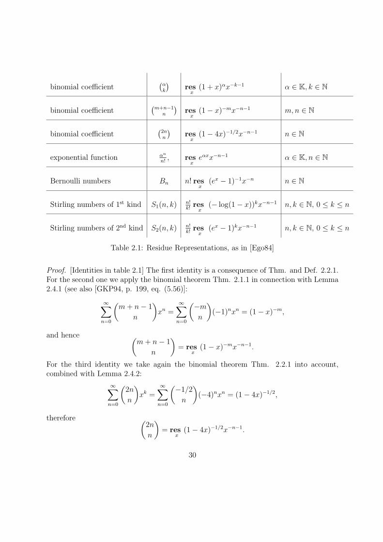
binomial coefficient(αk
)res
x(1 + x)αx−k−1 α ∈ K, k ∈ N
binomial coefficient(m+n−1
n
)res
x(1− x)−mx−n−1 m,n ∈ N
binomial coefficient(2nn
)res
x(1− 4x)−1/2x−n−1 n ∈ N
exponential function αn
n!, res
xeαxx−n−1 α ∈ K, n ∈ N
Bernoulli numbers Bn n! resx
(ex − 1)−1x−n n ∈ N
Stirling numbers of 1st kind S1(n, k)n!k!res
x(− log(1− x))kx−n−1 n, k ∈ N, 0 ≤ k ≤ n
Stirling numbers of 2nd kind S2(n, k)n!k!res
x(ex − 1)kx−n−1 n, k ∈ N, 0 ≤ k ≤ n
Table 2.1: Residue Representations, as in [Ego84]
Proof. [Identities in table 2.1] The first identity is a consequence of Thm. and Def. 2.2.1.For the second one we apply the binomial theorem Thm. 2.1.1 in connection with Lemma2.4.1 (see also [GKP94, p. 199, eq. (5.56)]:
∞∑n=0
(m+ n− 1
n
)xn =
∞∑n=0
(−m
n
)(−1)nxn = (1− x)−m,
and hence (m+ n− 1
n
)= res
x(1− x)−mx−n−1.
For the third identity we take again the binomial theorem Thm. 2.2.1 into account,combined with Lemma 2.4.2:
∞∑n=0
(2n
n
)xk =
∞∑n=0
(−1/2
n
)(−4)nxn = (1− 4x)−1/2,
therefore (2n
n
)= res
x(1− 4x)−1/2x−n−1.
30
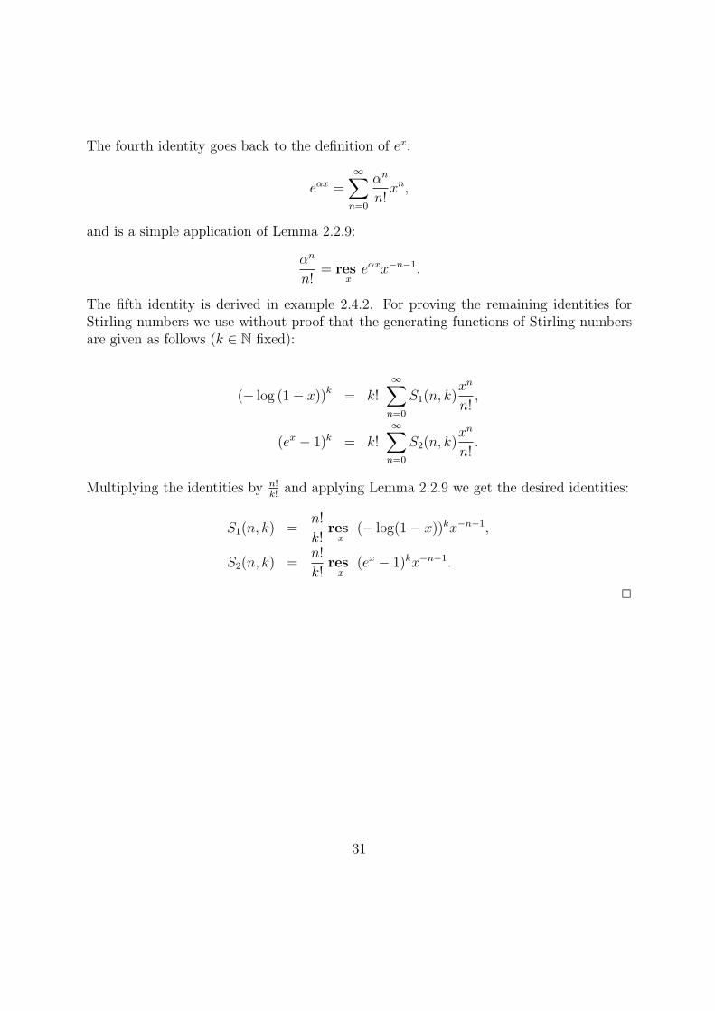
The fourth identity goes back to the definition of ex:
eαx =∞∑n=0
αn
n!xn,
and is a simple application of Lemma 2.2.9:
αn
n!= res
xeαxx−n−1.
The fifth identity is derived in example 2.4.2. For proving the remaining identities forStirling numbers we use without proof that the generating functions of Stirling numbersare given as follows (k ∈ N fixed):
(− log (1− x))k = k!∞∑n=0
S1(n, k)xn
n!,
(ex − 1)k = k!∞∑n=0
S2(n, k)xn
n!.
Multiplying the identities by n!k!
and applying Lemma 2.2.9 we get the desired identities:
S1(n, k) =n!
k!res
x(− log(1− x))kx−n−1,
S2(n, k) =n!
k!res
x(ex − 1)kx−n−1.
2
31
Chapter 3
The Riordan group
3.1 The Riordan array approach
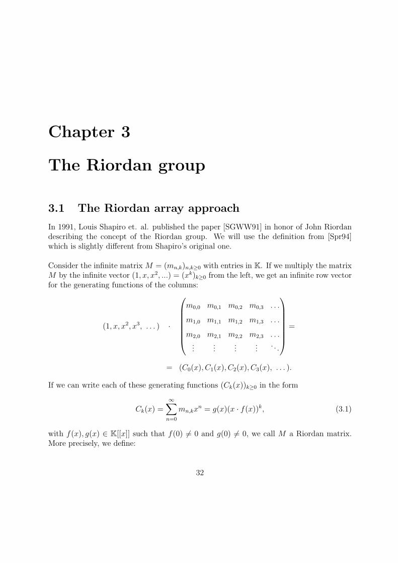
In 1991, Louis Shapiro et. al. published the paper [SGWW91] in honor of John Riordandescribing the concept of the Riordan group. We will use the definition from [Spr94]which is slightly different from Shapiro’s original one.
Consider the infinite matrix M = (mn,k)n,k≥0 with entries in K. If we multiply the matrixM by the infinite vector (1, x, x2, ...) = (xk)k≥0 from the left, we get an infinite row vectorfor the generating functions of the columns:
(1, x, x2, x3, . . . ) ·
m0,0 m0,1 m0,2 m0,3 . . .
m1,0 m1,1 m1,2 m1,3 . . .
m2,0 m2,1 m2,2 m2,3 . . ....
......
.... . .
=
= (C0(x), C1(x), C2(x), C3(x), . . . ).
If we can write each of these generating functions (Ck(x))k≥0 in the form
Ck(x) =∞∑n=0
mn,kxn = g(x)(x · f(x))k, (3.1)
with f(x), g(x) ∈ K[[x]] such that f(0) = 0 and g(0) = 0, we call M a Riordan matrix.More precisely, we define:
32
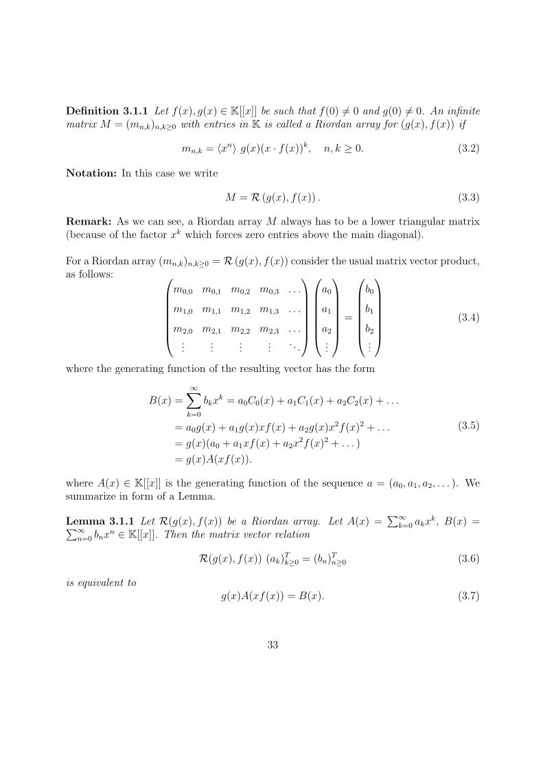
Definition 3.1.1 Let f(x), g(x) ∈ K[[x]] be such that f(0) = 0 and g(0) = 0. An infinitematrix M = (mn,k)n,k≥0 with entries in K is called a Riordan array for (g(x), f(x)) if
mn,k = ⟨xn⟩ g(x)(x · f(x))k, n, k ≥ 0. (3.2)
Notation: In this case we write
M = R (g(x), f(x)) . (3.3)
Remark: As we can see, a Riordan array M always has to be a lower triangular matrix(because of the factor xk which forces zero entries above the main diagonal).
For a Riordan array (mn,k)n,k≥0 = R (g(x), f(x)) consider the usual matrix vector product,as follows:
m0,0 m0,1 m0,2 m0,3 . . .
m1,0 m1,1 m1,2 m1,3 . . .
m2,0 m2,1 m2,2 m2,3 . . ....
......
.... . .
a0
a1
a2...
=
b0
b1
b2...
(3.4)
where the generating function of the resulting vector has the form
B(x) =∞∑k=0
bkxk = a0C0(x) + a1C1(x) + a2C2(x) + . . .
= a0g(x) + a1g(x)xf(x) + a2g(x)x2f(x)2 + . . .
= g(x)(a0 + a1xf(x) + a2x2f(x)2 + . . . )
= g(x)A(xf(x)).
(3.5)
where A(x) ∈ K[[x]] is the generating function of the sequence a = (a0, a1, a2, . . . ). Wesummarize in form of a Lemma.
Lemma 3.1.1 Let R(g(x), f(x)) be a Riordan array. Let A(x) =∑∞
k=0 akxk, B(x) =∑∞
n=0 bnxn ∈ K[[x]]. Then the matrix vector relation
R(g(x), f(x)) (ak)Tk≥0 = (bn)
Tn≥0 (3.6)
is equivalent tog(x)A(xf(x)) = B(x). (3.7)
33
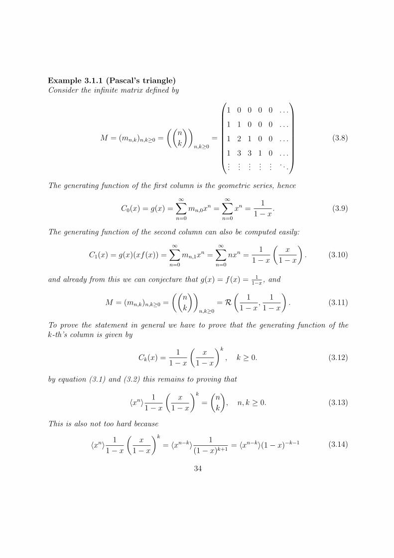
Example 3.1.1 (Pascal’s triangle)Consider the infinite matrix defined by
M = (mn,k)n,k≥0 =
((n
k
))n,k≥0
=
1 0 0 0 0 . . .
1 1 0 0 0 . . .
1 2 1 0 0 . . .
1 3 3 1 0 . . ....
......
......
. . .
(3.8)
The generating function of the first column is the geometric series, hence
C0(x) = g(x) =∞∑n=0
mn,0xn =
∞∑n=0
xn =1
1− x. (3.9)
The generating function of the second column can also be computed easily:
C1(x) = g(x)(xf(x)) =∞∑n=0
mn,1xn =
∞∑n=0
nxn =1
1− x
(x
1− x
). (3.10)
and already from this we can conjecture that g(x) = f(x) = 11−x
, and
M = (mn,k)n,k≥0 =
((n
k
))n,k≥0
= R(
1
1− x,
1
1− x
). (3.11)
To prove the statement in general we have to prove that the generating function of thek-th’s column is given by
Ck(x) =1
1− x
(x
1− x
)k
, k ≥ 0. (3.12)
by equation (3.1) and (3.2) this remains to proving that
⟨xn⟩ 1
1− x
(x
1− x
)k
=
(n
k
), n, k ≥ 0. (3.13)
This is also not too hard because
⟨xn⟩ 1
1− x
(x
1− x
)k
= ⟨xn−k⟩ 1
(1− x)k+1= ⟨xn−k⟩(1− x)−k−1 (3.14)
34
Now we have by the binomial theorem 2.1.1 that
(1− x)−k−1 =∞∑n=0
(−k − 1
n
)(−1)nxn,
and hence,
⟨xn−k⟩(1− x)−k−1 = (−1)n−k
(−k − 1
n− k
)=
(k + 1 + n− k − 1
n− k
)=
(n
n− k
)=
(n
k
),
where we used Lemma 2.4.1 and the elementary symmetry property.
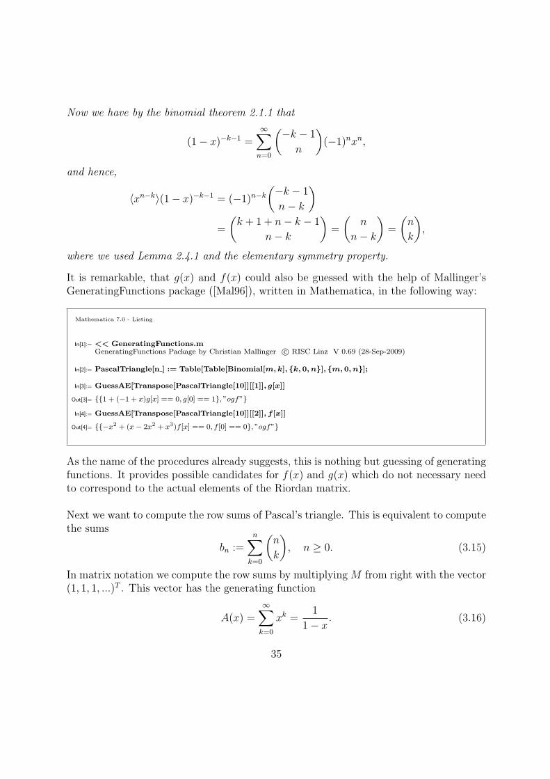
It is remarkable, that g(x) and f(x) could also be guessed with the help of Mallinger’sGeneratingFunctions package ([Mal96]), written in Mathematica, in the following way:
Mathematica 7.0 - Listing
In[1]:= << GeneratingFunctions.mGeneratingFunctions Package by Christian Mallinger c⃝ RISC Linz V 0.69 (28-Sep-2009)
In[2]:= PascalTriangle[n ] := Table[Table[Binomial[m,k], {k, 0, n}], {m, 0, n}];
In[3]:= GuessAE[Transpose[PascalTriangle[10]][[1]], g[x]]
Out[3]= {{1 + (−1 + x)g[x] == 0, g[0] == 1}, ”ogf”}
In[4]:= GuessAE[Transpose[PascalTriangle[10]][[2]], f [x]]
Out[4]= {{−x2 + (x− 2x2 + x3)f [x] == 0, f [0] == 0}, ”ogf”}
As the name of the procedures already suggests, this is nothing but guessing of generatingfunctions. It provides possible candidates for f(x) and g(x) which do not necessary needto correspond to the actual elements of the Riordan matrix.
Next we want to compute the row sums of Pascal’s triangle. This is equivalent to computethe sums
bn :=n∑
k=0
(n
k
), n ≥ 0. (3.15)
In matrix notation we compute the row sums by multiplying M from right with the vector(1, 1, 1, ...)T . This vector has the generating function
A(x) =∞∑k=0
xk =1
1− x. (3.16)
35
Hence, by relation (3.5) we find that
R(
1
1− x,
1
1− x
)1
1
1...
=
b0
b1
b2...
, (3.17)
i.e.,
B(x) =∞∑n=0
bnxn = g(x)A(xf(x)) (3.18)
where we apply the insertion homomorphism Φxf(x) to A(x) = (1−x)−1 as in Thm. 2.2.1,
=1
1− x· 1
1− x1−x
=1
1− 2x. (3.19)
Therefore for the nth row we find that
bn =n∑
k=0
(n
k
)= ⟨xn⟩ 1
1− 2x= 2n, n ≥ 0. (3.20)
The alternating row sum is multiplication of M by (1,−1, 1,−1, ...)T = ((−1)k)k≥0. Againwe get for A(x) a geometric series
A(x) =∞∑k=0
(−x)k =1
1 + x, (3.21)
and the relation
R(
1
1− x,
1
1− x
)
1
−1
1...
=
d0
d1
d2...
, (3.22)
Again (3.5), and application of the insertion homomorphism Φxf(x) to A(x) = (1 + x)−1
gives
D(x) =∞∑n=0
dnxn = g(x)A(xf(x)) =
1
1− x
1
1 + x1−x
= 1, n ≥ 0. (3.23)
We get the identityn∑
k=0
(−1)k(n
k
)= δ(n, 0), n ≥ 0. (3.24)
36
3.2 Characterization of Riordan arrays
Let RA denote the set of all Riordan arrays over K, i.e. the set of all infinite lowertriangular matrices with entries in K, that can be characterized in the way described inDef. 3.1.1. If M1 = R(g(x), f(x)) ∈ RA and M2 = R(h(x), l(x)) ∈ RA are two Riordanarrays, one might want to compute the usual matrix product (row by column - product)to obtain another Riordan array. So let
M1 = (an,k)n,k≥0, M2 = (bn,k)n,k≥0, (3.25)
such that
an,k = ⟨xn⟩g(x)(xf(x))k, (3.26)
bn,k = ⟨xn⟩h(x)(xl(x))k. (3.27)
We compute the matrix product
M := (cn,k) := M1 ·M2 = R (g(x), f(x)) · R (h(x), l(x)) , (3.28)
this means, computing the entry cn,k as for matrices,
cn,k =∞∑j=0
an,jbj,k. (3.29)
Let M = (M (0),M (1),M (2), ...), where
M (k) =
c0,k
c1,k
c2,k...
= kth column of M (3.30)
The generating function of the kth column is given by
M (k)(x) :=∞∑n=0
cn,kxn =
∞∑n=0
xn
(∞∑j=0
an,jbj,k
)=
∞∑j=0
bj,k
(∞∑n=0
an,jxn
)
=∞∑j=0
bj,kg(x)(xf(x))j = g(x)
∞∑j=0
bj,k(xf(x))j
Lemma 3.1.1= g(x)h(xf(x)) (xf(x)l(xf(x)))k
(3.31)
37
From this we can read off that the usual matrix product of Riordan arrays gives again aRiordan array as
· : RA×RA −→ RA,
(R(g(x), f(x))︸ ︷︷ ︸M1
,R(h(x), l(x))︸ ︷︷ ︸M2
) 7−→ M1 ·M2 (3.32)
whereM1 ·M2 = R(g(x)h(xf(x)), f(x)l(xf(x))) (3.33)
Obviously, the operation · : RA×RA → RA on the set of Riordan matrices is an asso-ciative binary operation.
It is also clear that the identity matrix I := R(1, 1) is the (right and left) neutral elementw.r.t ·.
If we now want to find an inverse element w.r.t. our operation · we consider the product
R(g(x), f(x)) · R(h(x), l(x)) = R(g(x)h(xf(x)), f(x)l(xf(x))) = R(1, 1). (3.34)
The formal power seriesF (x) := xf(x) (3.35)
has order 1, and by Thm. 2.2.4 a unique compositional inverse F ⟨−1⟩(x). Hence, wechoose h(x) and l(x) such that
h(x) :=1
g(F ⟨−1⟩(x)), (3.36)
l(x) :=1
f(F ⟨−1⟩(x)). (3.37)
If we plug this in, we find that
R(g(x), f(x)) · R(h(x), l(x))
(3.32)= R(g(x)h(xf(x)), f(x)l(xf(x)))
(3.35)= R(g(x)h(F (x)), f(x)l(F (x)))
(3.36),(3.37)= R
(g(x)
1
g(F ⟨−1⟩(F (x))), f(x)
1
f(F ⟨−1⟩(F (x)))
)(2.46)= R
(g(x)
1
g(x), f(x)
1
f(x)
)= R(1, 1).
The unique (right- and left-)inverse of a Riordan array R(g(x), f(x)), as we constructedit, will be denoted by R(g(x), f(x))−1.
38
Theorem 3.2.1The set of Riordan matrices RA with the operation · (short: (RA, ·)) is groupLet us examine, when an array (dn,k)n,k≥0 is a Riordan array.
Theorem 3.2.2 ([HS09], p. 3963, Thm. 2.1)An infinite lower triangular array D = (dn,k)n,k≥0 in K is a Riordan array if and only ifa sequence A = (a0 = 0, a1, a2, ...) in KN exists such that for every n, k ∈ N the followingrelation holds:
dn+1,k+1 = a0dn,k + a1dn,k+1 + a2dn,k+2 + . . . (3.38)
Remark: The sum is actually finite since dn,k = 0 for k > n.
Proof. ([Spr06, p. 58, Thm. 5.3.1]) ′′ ⇒′′: Let us suppose that D = (dn,k)n,k≥0 is theRiordan array R(g(x), f(x)), i.e.
dn,k = ⟨xn⟩g(x)(xf(x))k, (3.39)
and let us consider the Riordan array R(g(x)f(x), f(x)). We define the Riordan arrayR(A(x), B(x)) by the relation
R(A(x), B(x)) = R(g(x), f(x))−1 · R(g(x)f(x), f(x))
⇔ R(g(x), f(x)) · R(A(x), B(x)) = R(g(x)f(x), f(x)).
Because (RA, ·) is a group, the Riordan array R(A(x), B(x)) is well defined. We will latersee, that A(x) is the generating function of the sequence A. By performing the producton the left hand side we find that:
g(x)A(xf(x)) = g(x)f(x) and f(x)B(xf(x)) = f(x).
From the latter identity we get that B(xf(x)) = 1 ⇒ B(x) = 1. Therefore
R(g(x), f(x)) · R(A(x), 1) = R(g(x)f(x), f(x)).
The Riordan array on the left hand side is
R(g(x), f(x)) · R(A(x), 1) = R(g(x)A(xf(x)), f(x))
and its general element fn,k is
fn,k = ⟨xn⟩ g(x)A(xf(x))(xf(x))k
= ⟨xn⟩∞∑j=0
aj(xf(x))jg(x)(xf(x))k
Lem.2.2.8=
∞∑j=0
aj⟨xn⟩ g(x)(xf(x))k+j
(3.39)=
∞∑j=0
ajdn,k+j
39
The right hand side evaluates to:
⟨xn⟩ g(x)f(x)(x(f(x))k = ⟨xn+1⟩ xg(x)f(x)(xf(x))k = dn+1,k+1.
By equating these two quantities, we get the identity (3.38).
′′ ⇐′′: If the first column of a Riordan matrix (i.e. the sequence of elements (dk,0)k≥0) isgiven, relation (3.38) constructs the Riordan matrix recursively (by repeated applicationof (3.38)). Let g(x) be the generating function of the first column (we assume d0,0 is notzero), A(x) the generating function of the sequence A = (ak)k≥0. Consider the functionalequation (recall that F (x) := xf(x))
f(x) = A(F (x)), (3.40)
where f(x) ∈ K0((x)). Then, F (x) has order 1, and by Thm. 2.2.4 a unique compositionalinverse F ⟨−1⟩(x) exists. In particular, (3.40) implies that
A(x) = f(F ⟨−1⟩(x)). (3.41)
Therefore we can consider the Riordan array
D := R(g(x), f(x))
The generating function of the first column coincide by construction, the generating func-tion for the kth column match by recurrence relation (3.38). 2
The sequenceA = (ak)k≥0 is called theA− sequence of the Riordan arrayD = R(g(x), f(x)).As we have seen in the proof of the theorem, its generating function A(x) =
∑∞k=0 akx
k,satisfies the functional equation
f(x) = A(xf(x)), (3.42)
and it only depends on f(x).Conversely, A(x) can be determined by the relation:
A(x) = f(F ⟨−1⟩(x)), where F (x) := xf(x). (3.43)
Another type of characterization is obtained through the following observation
Theorem 3.2.3 ([Spr06] p. 58, Thm. 5.3.2)Let M := (dn,k)n,k≥0 = R(g(x), f(x)) be a Riordan array. Then a unique sequence Z =(zk)k≥0 exists such that every element in column 0 can be expressed as a linear combinationof all the elements in the preceding row, i.e.
dn+1,0 = z0dn,0 + z1dn,1 + z2dn,2 + . . . (3.44)
40
Proof. Let z0 = d1,0d0,0
. Now, due to the fact that (dn,k)n,k≥0 is a lower triangular matrix,
we can uniquely determine the value of z1 by expressing d2,0 in terms of the elements inrow 1, i.e.
d2,0 = z0d1,0 + z1d1,1 ⇔ z1 =d0,0d2,0 − d21,0
d0,0d1,1.
In the same way, we determine z2 by expressing d3,0 in terms of the elements in row 2,and by substituting the values just obtained for z0 and z1. By proceeding the same way,we determine the sequence Z in a unique way. 2
The sequence Z is called the Z−sequence for the Riordan array. It characterizes column0 except for the first element. Let A(t) =
∑∞k=0 akt
k be the generating function of theA-sequence (ak)k≥0, Z(t) =
∑∞k=0 zkt
k the generating function of the Z-sequence (zk)k≥0.For d0,0 ∈ K\{0}, we can say that the triple
(d0,0, A(t), Z(t))
completely characterizes a Riordan array. The next theorem is a way how to computeg(x) given f(x) and the Z−sequence of a Riordan array.
Theorem 3.2.4 ([MRSV97], p. 5, Thm. 2.3)Let M = (dn,k)n,k≥0 = R(g(x), f(x)) be a Riordan array and let Z(t) =
∑∞n=0 znt
n be thegenerating function of the array’s Z−sequence (zk)k≥0. Then:
g(x) =g(0)
1− xZ(xf(x)). (3.45)
Proof. By the preceding Theorem, the Z−sequence exists and is unique, and equation(3.44) is valid for every n ∈ N. Relation (3.44) translates to
dn+1,0 = z0dn,0 + z1dn,1 + z2dn,2 + . . .
⟨xn+1⟩g(x) =∞∑k=0
zk⟨xn⟩g(x)(xf(x))k
⟨xn⟩g(x)− g(0)
x= ⟨xn⟩g(x)Z(xf(x))
Because two power series are identical if and only if their coefficients coincide, we haveequality above, because the last line holds for all n ∈ N. Hence, we find that
g(x)− g(0)
x= g(x)Z(xf(x)) ⇔ g(x) =
g(0)
1− xZ(xf(x)).
2
41
Note: This relation can be inverted and this gives us a formula for the generating functionof the Z−sequence (F (x) := xf(x)):
g(x)− g(0)
xg(x)= Z(xf(x)) ⇒ Z(y) =
g(F ⟨−1⟩(x))− g(0)
F ⟨−1⟩(x)g(F ⟨−1⟩(x)). (3.46)
There is a non-trivial connection between the generating functions of the A− and the Z−sequence and the functions g(x) and f(x). In particular the following holds:
Theorem 3.2.5 ([MRSV97], p. 6, Thm. 2.4)Let D = R(g(x), f(x)) ∈ RA. Then g(x) = f(x) if and only if A(x) = g(0) + xZ(x)
Proof. ′′ ⇐′′: Let us assume that A(x) = g(0) + xZ(x) or what is the same Z(x) =(A(x)− g(0))/x. By the preceding theorem we have
g(x) =g(0)
1− xZ(xf(x))=
g(0)
1− (xA(xf(x))− g(0)x)/(xf(x))=
g(0)xf(x)
g(0)x= f(x),
because, by (3.42) we have that A(xf(x)) = f(x).
′′ ⇒′′: By (3.45) and from the hypothesis g(x) = f(x) we find that:
g(x) =g(0)
1− xZ(xf(x))=
g(0)
1− xZ(xg(x))
⇔ g(x)− xg(x)Z(xg(x)) = g(0).
Now we apply (3.42) and the hypothesis:
f(x) = A(xf(x)) ⇒ g(x) = A(xg(x)),
to obtain the identity:A(xg(x)) = g(0) + xg(x)Z(xg(x)).
or, with G(x) := xg(x):A(G(x)) = g(0) +G(x)Z(G(x)).
Setting x = G⟨−1⟩(x) gives the desired equality. 2
42
Chapter 4
Application to Symbolic Summation
4.1 The Identities of Abel and Gould
Wilf and Zeilberger provide an algorithm for proving summation identities of the form∑k
summand(n, k) = answer(n), n ≥ 0. (4.1)
where summand(n, k) and answer(n) are nice.
For a given sum
f(n) =∑k
F (n, k), (4.2)
where F is doubly hypergeometric (that is both F (n+1, k)/F (n, k) and F (n, k+1)/F (n, k)are rational functions of n and k) every proper hypergeometric term F (n, k) satisfies ak-free recurrence [PWZ96, Thm. 4.4.1, p. 65]. A proper hypergeometric term can bewritten in the form
P (n, k)
∏ui=0(ain+ bik + ci)!∏vi=0(uin+ vik + wi)!
xk, (4.3)
where P (n, k) ∈ K[n, k], x ∈ K, an, bn, un, vn ∈ N, u, v ∈ N.
So there exist I, J ∈ N and polynomials ai,j(n) such that the recurrence
I∑i=0
J∑j=0
ai,j(n)F (n− j, k − i) = 0 (4.4)
holds at every point (n, k) where F (n, k) = 0. Further there are bounds for I, J given.
43
However, there are combinatorial sums that are not doubly hypergeometric in the sensedefined above. For instance, if we try to prove the identity of Abel ([GKP94, p. 202,(5.64)])
n∑k=0
(n
k
)a(a+ k)k−1(b+ n− k)n−k = (a+ b+ n)n, a, b ∈ K, n ≥ 0. (4.5)
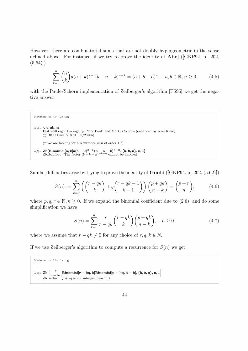
with the Paule/Schorn implementation of Zeilberger’s algorithm [PS95] we get the nega-tive answer
Mathematica 7.0 - Listing
In[1]:= << zb.mFast Zeilberger Package by Peter Paule and Markus Schorn (enhanced by Axel Riese)c⃝ RISC Linz V 3.54 (02/23/05)
(* We are looking for a recurrence in n of order 1 *)
In[2]:= Zb[Binomial[n, k]a(a + k)k−1(b + n − k)n−k, {k, 0, n}, n, 1]Zb::badfac : The factor (b− k + n)−k+n cannot be handled
Similar difficulties arise by trying to prove the identity of Gould ([GKP94, p. 202, (5.62)])
S(n) :=n∑
k=0
((r − qk
k
)+ q
(r − qk − 1
k − 1
))(p+ qk
n− k
)=
(p+ r
n
), (4.6)
where p, q, r ∈ N, n ≥ 0. If we expand the binomial coefficient due to (2.6), and do somesimplification we have
S(n) =n∑
k=0
r
r − qk
(r − qk
k
)(p+ qk
n− k
), n ≥ 0, (4.7)
where we assume that r − qk = 0 for any choice of r, q, k ∈ N.
If we use Zeilberger’s algorithm to compute a recurrence for S(n) we get
Mathematica 7.0 - Listing
In[1]:= Zb
[r
r − kqBinomial[r − kq, k]Binomial[p + kq, n − k], {k, 0, n}, n, 1
]Zb::intlin : p+ kq is not integer-linear in k
44
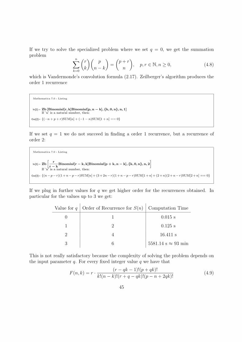
If we try to solve the specialized problem where we set q = 0, we get the summationproblem
n∑k=0
(r
k
)(p
n− k
)=
(p+ r
n
), p, r ∈ N, n ≥ 0, (4.8)
which is Vandermonde’s convolution formula (2.17). Zeilberger’s algorithm produces theorder 1 recurrence
Mathematica 7.0 - Listing
In[2]:= Zb [Binomial[r, k]Binomial[p, n − k], {k, 0, n}, n, 1]If ’n’ is a natural number, then:
Out[2]= {(−n+ p+ r)SUM[n] + (−1− n)SUM[1 + n] == 0}
If we set q = 1 we do not succeed in finding a order 1 recurrence, but a recurrence oforder 2:
Mathematica 7.0 - Listing
In[3]:= Zb
[r
r − kBinomial[r − k, k]Binomial[p + k, n − k], {k, 0, n}, n, 2
]If ’n’ is a natural number, then:
Out[3]= {(n− p− r)(1+n− p− r)SUM[n] + (3+2n− r)(1+n− p− r)SUM[1+n] + (2+n)(2+n− r)SUM[2+n] == 0}
If we plug in further values for q we get higher order for the recurrences obtained. Inparticular for the values up to 3 we get:
Value for q Order of Recurrence for S(n) Computation Time
0 1 0.015 s
1 2 0.125 s
2 4 16.411 s
3 6 5581.14 s ≈ 93 min
This is not really satisfactory because the complexity of solving the problem depends onthe input parameter q. For every fixed integer value q we have that
F (n, k) = r · (r − qk − 1)!(p+ qk)!
k!(n− k)!(r + q − qk)!(p− n+ 2qk)!(4.9)
45
is a proper hypergeometric term, and therefore f(n) =∑
k F (n, k) satisfies a k-free re-currence. In the following, we present ways of how to compute the sum for general q.
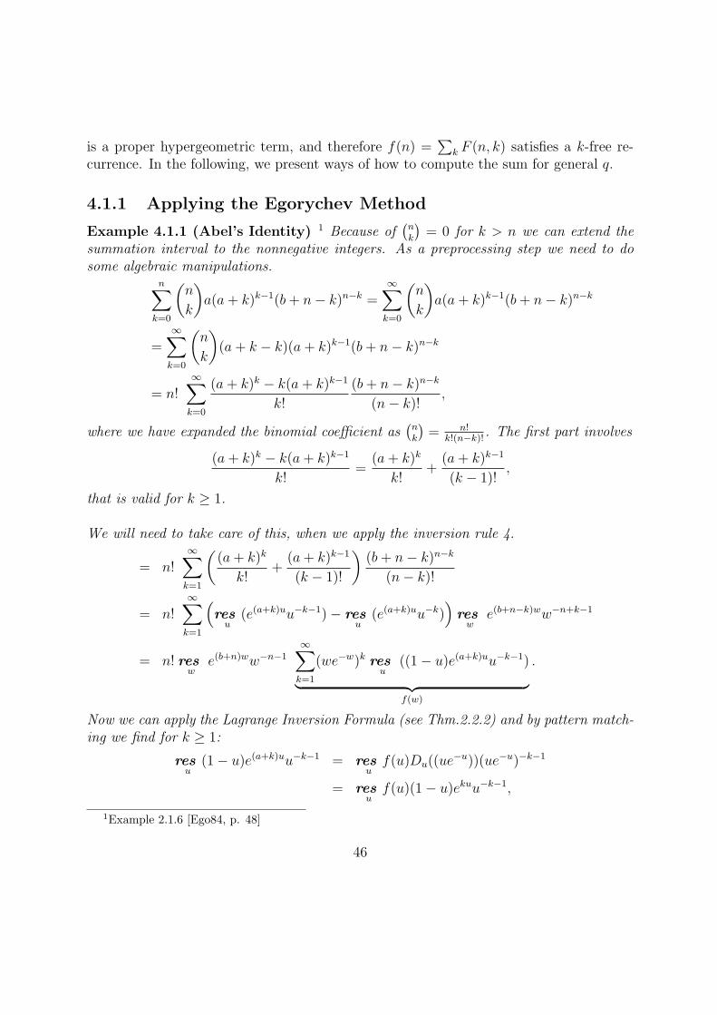
4.1.1 Applying the Egorychev Method
Example 4.1.1 (Abel’s Identity) 1 Because of(nk
)= 0 for k > n we can extend the
summation interval to the nonnegative integers. As a preprocessing step we need to dosome algebraic manipulations.
n∑k=0
(n
k
)a(a+ k)k−1(b+ n− k)n−k =
∞∑k=0
(n
k
)a(a+ k)k−1(b+ n− k)n−k
=∞∑k=0
(n
k
)(a+ k − k)(a+ k)k−1(b+ n− k)n−k
= n!∞∑k=0
(a+ k)k − k(a+ k)k−1
k!
(b+ n− k)n−k
(n− k)!,
where we have expanded the binomial coefficient as(nk
)= n!
k!(n−k)!. The first part involves
(a+ k)k − k(a+ k)k−1
k!=
(a+ k)k
k!+
(a+ k)k−1
(k − 1)!,
that is valid for k ≥ 1.
We will need to take care of this, when we apply the inversion rule 4.
= n!∞∑k=1
((a+ k)k
k!+
(a+ k)k−1
(k − 1)!
)(b+ n− k)n−k
(n− k)!
= n!∞∑k=1
(res
u(e(a+k)uu−k−1)− res
u(e(a+k)uu−k)
)res
we(b+n−k)ww−n+k−1
= n! resw
e(b+n)ww−n−1
∞∑k=1
(we−w)k resu
((1− u)e(a+k)uu−k−1)︸ ︷︷ ︸f(w)
.
Now we can apply the Lagrange Inversion Formula (see Thm.2.2.2) and by pattern match-ing we find for k ≥ 1:
resu
(1− u)e(a+k)uu−k−1 = resu
f(u)Du((ue−u))(ue−u)−k−1
= resu
f(u)(1− u)ekuu−k−1,
1Example 2.1.6 [Ego84, p. 48]
46
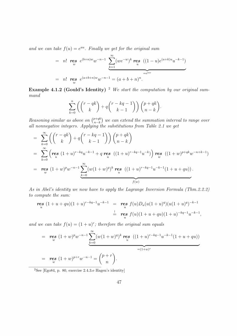
and we can take f(u) = eau. Finally we get for the original sum
= n! resw
e(b+n)ww−n−1
∞∑k=1
(we−w)k resu
((1− u)e(a+k)uu−k−1)︸ ︷︷ ︸=eaw
= n! resw
e(a+b+n)ww−n−1 = (a+ b+ n)n.
Example 4.1.2 (Gould’s Identity) 2 We start the computation by our original sum-mand
n∑k=0
((r − qk
k
)+ q
(r − kq − 1
k − 1
))(p+ qk
n− k
).
Reasoning similar as above on(p+qkn−k
)we can extend the summation interval to range over
all nonnegative integers. Applying the substitutions from Table 2.1 we get
=∞∑k=0
((r − qk
k
)+ q
(r − kq − 1
k − 1
))(p+ qk
n− k
)=
∞∑k=0
(res
u(1 + u)r−kqu−k−1 + q res
u((1 + u)r−kq−1u−k)
)res
w((1 + w)p+qkw−n+k−1)
= resw
(1 + w)pw−n−1
∞∑k=0
(w(1 + w)q)k resu
((1 + u)r−kq−1u−k−1(1 + u+ qu))︸ ︷︷ ︸f(w)
.
As in Abel’s identity we now have to apply the Lagrange Inversion Formula (Thm.2.2.2)to compute the sum:
resu
(1 + u+ qu)(1 + u)r−kq−1u−k−1 = resu
f(u)Du(u(1 + u)q)(u(1 + u)q)−k−1
!= res
uf(u)(1 + u+ qu)(1 + u)−kq−1u−k−1,
and we can take f(u) = (1 + u)r; therefore the original sum equals
= resw
(1 + w)pw−n−1
∞∑k=0
(w(1 + w)q)k resu
((1 + u)r−kq−1u−k−1(1 + u+ qu))︸ ︷︷ ︸=(1+w)r
= resw
(1 + w)p+rw−n−1 =
(p+ r
n
).
2See [Ego84, p. 80, exercise 2.4.3.e Hagen’s identity]
47
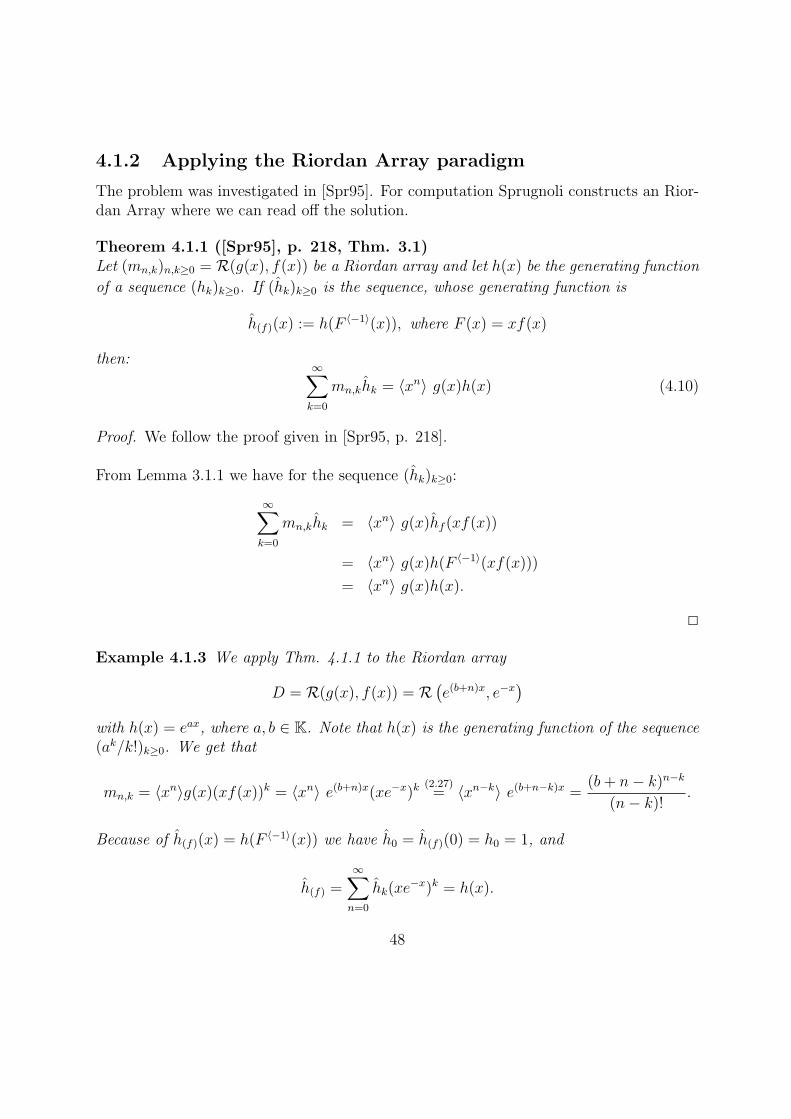
4.1.2 Applying the Riordan Array paradigm
The problem was investigated in [Spr95]. For computation Sprugnoli constructs an Rior-dan Array where we can read off the solution.
Theorem 4.1.1 ([Spr95], p. 218, Thm. 3.1)Let (mn,k)n,k≥0 = R(g(x), f(x)) be a Riordan array and let h(x) be the generating function
of a sequence (hk)k≥0. If (hk)k≥0 is the sequence, whose generating function is
h(f)(x) := h(F ⟨−1⟩(x)), where F (x) = xf(x)
then:∞∑k=0
mn,khk = ⟨xn⟩ g(x)h(x) (4.10)
Proof. We follow the proof given in [Spr95, p. 218].
From Lemma 3.1.1 we have for the sequence (hk)k≥0:
∞∑k=0
mn,khk = ⟨xn⟩ g(x)hf (xf(x))
= ⟨xn⟩ g(x)h(F ⟨−1⟩(xf(x)))
= ⟨xn⟩ g(x)h(x).
2
Example 4.1.3 We apply Thm. 4.1.1 to the Riordan array
D = R(g(x), f(x)) = R(e(b+n)x, e−x
)with h(x) = eax, where a, b ∈ K. Note that h(x) is the generating function of the sequence(ak/k!)k≥0. We get that
mn,k = ⟨xn⟩g(x)(xf(x))k = ⟨xn⟩ e(b+n)x(xe−x)k(2.27)= ⟨xn−k⟩ e(b+n−k)x =
(b+ n− k)n−k
(n− k)!.
Because of h(f)(x) = h(F ⟨−1⟩(x)) we have h0 = h(f)(0) = h0 = 1, and
h(f) =∞∑n=0
hk(xe−x)k = h(x).
48
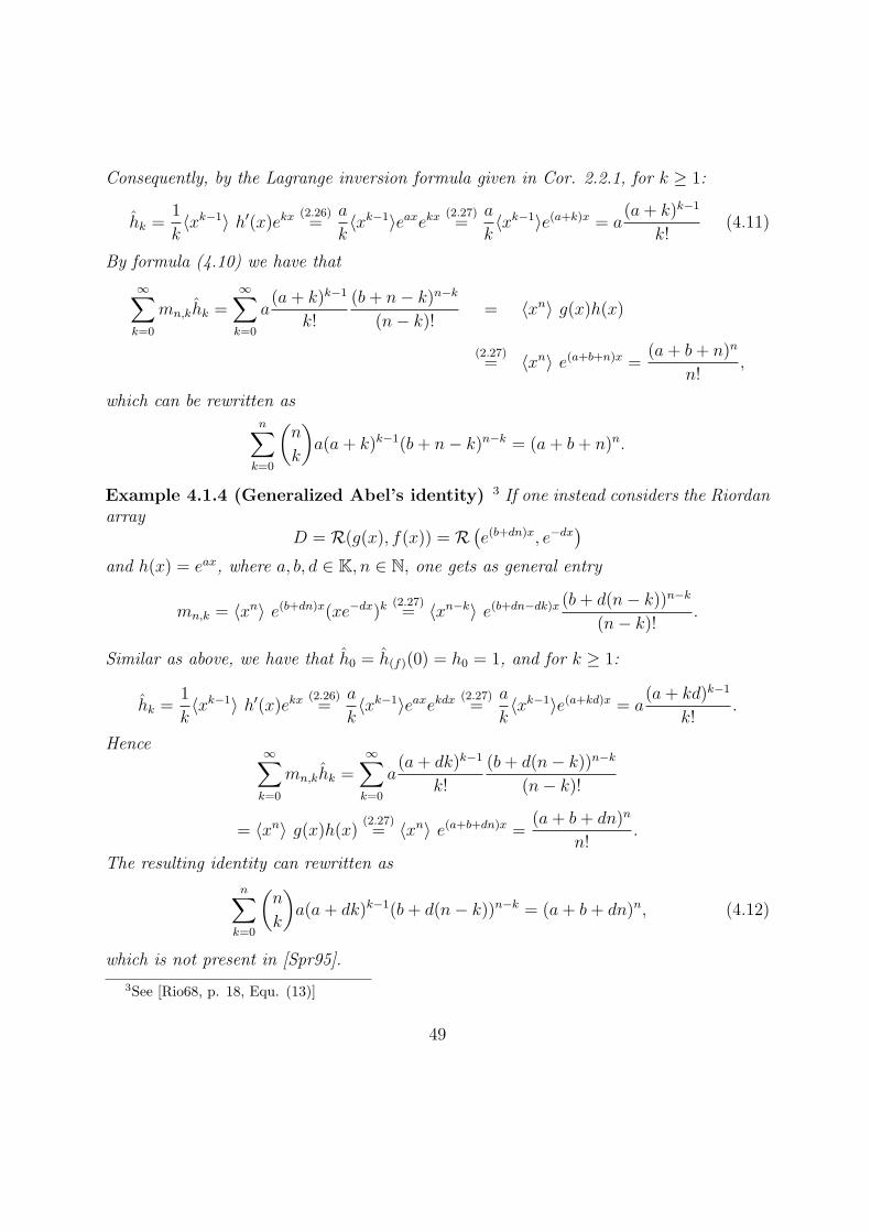
Consequently, by the Lagrange inversion formula given in Cor. 2.2.1, for k ≥ 1:
hk =1
k⟨xk−1⟩ h′(x)ekx
(2.26)=
a
k⟨xk−1⟩eaxekx (2.27)
=a
k⟨xk−1⟩e(a+k)x = a
(a+ k)k−1
k!(4.11)
By formula (4.10) we have that
∞∑k=0
mn,khk =∞∑k=0
a(a+ k)k−1
k!
(b+ n− k)n−k
(n− k)!= ⟨xn⟩ g(x)h(x)
(2.27)= ⟨xn⟩ e(a+b+n)x =
(a+ b+ n)n
n!,
which can be rewritten asn∑
k=0
(n
k
)a(a+ k)k−1(b+ n− k)n−k = (a+ b+ n)n.
Example 4.1.4 (Generalized Abel’s identity) 3 If one instead considers the Riordanarray
D = R(g(x), f(x)) = R(e(b+dn)x, e−dx
)and h(x) = eax, where a, b, d ∈ K, n ∈ N, one gets as general entry
mn,k = ⟨xn⟩ e(b+dn)x(xe−dx)k(2.27)= ⟨xn−k⟩ e(b+dn−dk)x (b+ d(n− k))n−k
(n− k)!.
Similar as above, we have that h0 = h(f)(0) = h0 = 1, and for k ≥ 1:
hk =1
k⟨xk−1⟩ h′(x)ekx
(2.26)=
a
k⟨xk−1⟩eaxekdx (2.27)
=a
k⟨xk−1⟩e(a+kd)x = a
(a+ kd)k−1
k!.
Hence∞∑k=0
mn,khk =∞∑k=0
a(a+ dk)k−1
k!
(b+ d(n− k))n−k
(n− k)!
= ⟨xn⟩ g(x)h(x) (2.27)= ⟨xn⟩ e(a+b+dn)x =
(a+ b+ dn)n
n!.
The resulting identity can rewritten as
n∑k=0
(n
k
)a(a+ dk)k−1(b+ d(n− k))n−k = (a+ b+ dn)n, (4.12)
which is not present in [Spr95].
3See [Rio68, p. 18, Equ. (13)]
49
Example 4.1.5 Consider the Riordan array
D = R(g(x), f(x)) = R ((1 + x)p, (1 + x)q) , p, q ∈ N,
and h(x) = (1 + x)r, where r ∈ N. By Thm. 4.1.1 we obtain that
mn,k = ⟨xn⟩ (1 + x)p(x(1 + x)q)k = ⟨xn−k⟩ (1 + x)p+qk =
(p+ qk
n− k
).
Furthermore, h0 = h(f)(0) = h0 = 1 and
hk =1
k⟨xk−1⟩ h′(x)f(x)−k =
1
k⟨xk−1⟩ Dx((1 + x)r)((1 + x)q)−k
(2.28),(2.16)=
r
k⟨xk−1⟩ (1 + x)r−1−qk =
r
k
(r − 1− qk
k − 1
)=
r
r − qk
(r − qk
k
)So we finally find
n∑k=0
r
r − qk
(r − qk
k
)(p+ qk
n− k
)= ⟨xn⟩ g(x)h(x) (2.16)
= ⟨xn⟩ (1 + x)p+r =
(p+ r
n
).
4.2 Multi-Sum Identities
The machinery developed by Egorychev is not restricted to one single summation quan-tifier as the following American Mathematical Monthly Problem shows.
Example: The American Mathematical Monthly, Problem 11033.4
Proposed by M.N. Deshpande and R.M. Welukar, Institute of Science, Nagpur, India.Let
P (m,n, r) :=r∑
k=0
(−1)k(m+ n− 2(k + 1)
n
)(r
k
)(4.13)
Let m,n and r be integers such that 0 ≤ r ≤ n ≤ m− 2. Show that P (m,n, r) is positiveand that
n∑r=0
P (m,n, r) =
(m+ n
n
)(4.14)
We start by considering the inner sum P (m,n, r). The summation over k can be extendedto range over the nonnegative integers because the binomial coefficient forces the summand
4The American Mathematical Monthly, Vol. 110, No. 8 (Oct., 2003), p. 742
50
to vanish identically for k > r. Afterwards we can replace the binomial coefficient by ourresidue functional.
P (m,n, r) =r∑
k=0
(−1)k(m+ n− 2(k + 1)
n
)(r
k
)=
∞∑k=0
(−1)k(m+ n− 2(k + 1)
n
)(r
k
)=
∞∑k=0
(−1)k resu
(1 + u)m+n−2−2ku−n−1 resw
(1 + w)rw−k−1
= resu
(1 + u)m+n−2u−n−1
∞∑k=0
(−(1 + u)−2)k resw
(1 + w)rw−k−1.
after pulling out the factors not depending on the summation index. Now we can takeinto account the substitution rule 3. The remaining sums simplifies to
∞∑k=0
(−(1 + u)−2)k resw
(1 + w)rw−k−1 =
(1− 1
(1 + u)2
)r
.
This gives us for the inner sum the residue representation
P (m,n, r) = resu
(1 + u)m+n−2−2rur(2 + u)ru−n−1. (4.15)
The BSI Problems Group, Bonn, Germany claimed in their solution5 of the problem thatthe original sum P (m,n, r) can be rewritten in the following way
r∑k=0
(−1)k(m+ n− 2(k + 1)
n
)(r
k
)=
m−2∑k=0
(r
k
)(n− r +m− 2− k
n− r
). (4.16)
If this is the case we have proven that P (m,n, r) is indeed positive since we are addingup non-negative quantities. (Note that by the assumptions on m,n, r the quantityn − r + m − 2 − k for 0 ≤ k ≤ m − 2 is always positive and so is the binomial coef-ficient (i.e. Lemma 2.4.1 is never invoked)).
We will present two proofs: The first one takes into account that the summands are bothhypergeometric. Hence, with the help of Zeilberger’s algorithm we can find recurrencerelations for the free variables r,m, n of both sums. If they coincide (up to a constantmultiple) it remains to check initial values to ensure equivalence.
5The American Mathematical Monthly, Vol. 112, No. 5 (May, 2005), p. 471, ”Expansion By Inclusion-Exclusion”
51
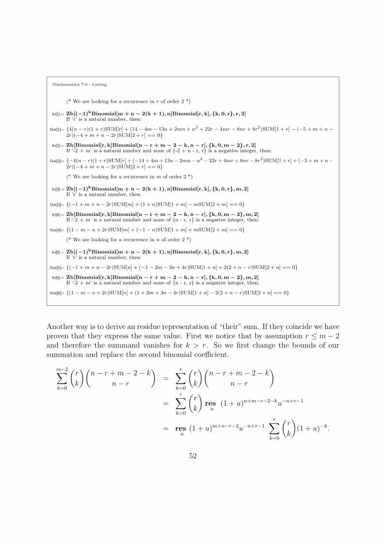
Mathematica 7.0 - Listing
(* We are looking for a recurrence in r of order 2 *)
In[1]:= Zb[(−1)kBinomial[m + n − 2(k + 1), n]Binomial[r, k], {k, 0, r}, r, 2]If ’r’ is a natural number, then:
Out[1]= {4(n − r)(1 + r)SUM[r] + (14 − 4m − 13n + 2mn + n2 + 22r − 4mr − 8nr + 8r2)SUM[1 + r] − (−5 + m + n −2r)(−4 +m+ n− 2r)SUM[2 + r] == 0}
In[2]:= Zb[Binomial[r, k]Binomial[n − r + m − 2 − k, n − r], {k, 0,m − 2}, r, 2]If ‘-2 + m’ is a natural number and none of {-2 + n - r, r} is a negative integer, then:
Out[2]= {−4(n− r)(1 + r)SUM[r] + (−14+ 4m+13n− 2mn− n2 − 22r+4mr+8nr− 8r2)SUM[1+ r] + (−5+m+ n−2r)(−4 +m+ n− 2r)SUM[2 + r] == 0}
(* We are looking for a recurrence in m of order 2 *)
In[3]:= Zb[(−1)kBinomial[m + n − 2(k + 1), n]Binomial[r, k], {k, 0, r},m, 2]If ’r’ is a natural number, then:
Out[3]= {(−1 +m+ n− 2r)SUM[m] + (1 + n)SUM[1 +m]−mSUM[2 +m] == 0}
In[4]:= Zb[Binomial[r, k]Binomial[n − r + m − 2 − k, n − r], {k, 0,m − 2},m, 2]If ‘-2 + m’ is a natural number and none of {n - r, r} is a negative integer, then:
Out[4]= {(1−m− n+ 2r)SUM[m] + (−1− n)SUM[1 +m] +mSUM[2 +m] == 0}
(* We are looking for a recurrence in n of order 2 *)
In[5]:= Zb[(−1)kBinomial[m + n − 2(k + 1), n]Binomial[r, k], {k, 0, r},m, 2]If ’r’ is a natural number, then:
Out[5]= {(−1 +m+ n− 2r)SUM[n] + (−1− 2m− 3n+ 4r)SUM[1 + n] + 2(2 + n− r)SUM[2 + n] == 0}
In[6]:= Zb[Binomial[r, k]Binomial[n − r + m − 2 − k, n − r], {k, 0,m − 2},m, 2]If ‘-2 + m’ is a natural number and none of {n - r, r} is a negative integer, then:
Out[6]= {(1−m− n+ 2r)SUM[n] + (1 + 2m+ 3n− 4r)SUM[1 + n]− 2(2 + n− r)SUM[2 + n] == 0}
Another way is to derive an residue representation of “their” sum. If they coincide we haveproven that they express the same value. First we notice that by assumption r ≤ m− 2and therefore the summand vanishes for k > r. So we first change the bounds of oursummation and replace the second binomial coefficient.
m−2∑k=0
(r
k
)(n− r +m− 2− k
n− r
)=
r∑k=0
(r
k
)(n− r +m− 2− k
n− r
)=
r∑k=0
(r
k
)res
u(1 + u)n+m−r−2−ku−n+r−1
= resu
(1 + u)m+n−r−2u−n+r−1
r∑k=0
(r
k
)(1 + u)−k.
52
Now apply the binomial theorem and get
resu
(1 + u)m+n−r−2u−n+r−1
r∑k=0
(r
k
)(1 + u)−k = res
u(1 + u)m+n−r−2u−n+r−1
(1 +
1
1 + u
)r
= resu
(1 + u)m+n−2−2rur (2 + u)r u−n−1,
in accordance with (4.15). This proves identity (4.16). We note that identity (4.16) couldbe derived by reading our proof of (4.16) backwards.
Finally we note that the identity (4.14) we want to prove here is in fact not very hardonce we plug in (4.15). We pull out the factors not depending on r and remain with asimple geometric series.
S(m,n) :=n∑
r=0
P (m,n, r) =n∑
r=0
resu
(1 + u)m+n−2−2rur(2 + u)ru−n−1
= resu
(1 + u)m+n−2u−n−1
n∑r=0
(u(2 + u)
(1 + u)2
)r
.
The geometric series evaluates to
n∑r=0
(u(2 + u)
(1 + u)2
)r
= (1 + u)2 − un+1(2 + u)n+1(1 + u)−2n,
and hence
S(m,n) = resu
(1 + u)m+nu−n−1 + resu
(1 + u)m−n−2(2 + u)n+1 =
(m+ n
n
)+ 0,
because by assumption m ≥ n+ 2.
2
4.3 Another Mathematical Monthly Problem
Manuel Kauers together with Sheng-Lang Ko came in their work to meet the sum
S(n) := (−1)nn∑
k=0
(−1)k(
2n
n+ k
)S1(n+ k, k). (4.17)
53
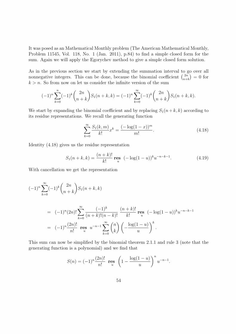
It was posed as an Mathematical Monthly problem (The American Mathematical Monthly,Problem 11545, Vol. 118, No. 1 (Jan. 2011), p.84) to find a simple closed form for thesum. Again we will apply the Egorychev method to give a simple closed form solution.
As in the previous section we start by extending the summation interval to go over allnonnegative integers. This can be done, because the binomial coefficient
(2nn+k
)= 0 for
k > n. So from now on let us consider the infinite version of the sum
(−1)nn∑
k=0
(−1)k(
2n
n+ k
)S1(n+ k, k) = (−1)n
∞∑k=0
(−1)k(
2n
n+ k
)S1(n+ k, k).
We start by expanding the binomial coefficient and by replacing S1(n+k, k) according toits residue representations. We recall the generating function
∞∑k=0
S1(k,m)
k!xk =
(− log(1− x))m
m!. (4.18)
Identity (4.18) gives us the residue representation
S1(n+ k, k) =(n+ k)!
k!res
u(− log(1− u))ku−n−k−1. (4.19)
With cancellation we get the representation
(−1)n∞∑k=0
(−1)k(
2n
n+ k
)S1(n+ k, k)
= (−1)n(2n)!∞∑k=0
(−1)k
(n+ k)!(n− k)!
(n+ k)!
k!res
u(− log(1− u))ku−n−k−1
= (−1)n(2n)!
n!res
uu−n−1
∞∑k=0
(n
k
)(− log(1− u)
u
)k
.
This sum can now be simplified by the binomial theorem 2.1.1 and rule 3 (note that thegenerating function is a polynomial) and we find that
S(n) = (−1)n(2n)!
n!res
u
(1− log(1− u)
u
)n
u−n−1.
54
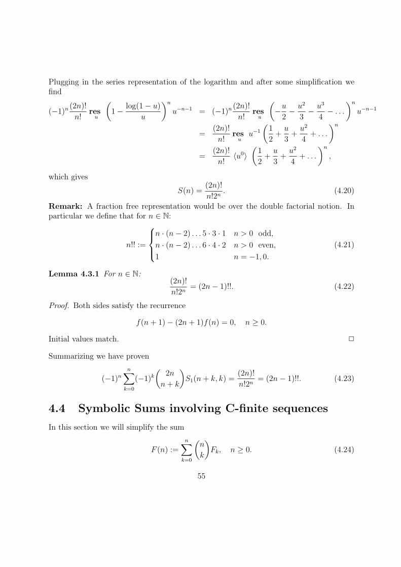
Plugging in the series representation of the logarithm and after some simplification wefind
(−1)n(2n)!
n!res
u
(1− log(1− u)
u
)n
u−n−1 = (−1)n(2n)!
n!res
u
(−u
2− u2
3− u3
4− . . .
)n
u−n−1
=(2n)!
n!res
uu−1
(1
2+
u
3+
u2
4+ . . .
)n
=(2n)!
n!⟨u0⟩
(1
2+
u
3+
u2
4+ . . .
)n
,
which gives
S(n) =(2n)!
n!2n. (4.20)
Remark: A fraction free representation would be over the double factorial notion. Inparticular we define that for n ∈ N:
n!! :=
n · (n− 2) . . . 5 · 3 · 1 n > 0 odd,
n · (n− 2) . . . 6 · 4 · 2 n > 0 even,
1 n = −1, 0.
(4.21)
Lemma 4.3.1 For n ∈ N:(2n)!
n!2n= (2n− 1)!!. (4.22)
Proof. Both sides satisfy the recurrence
f(n+ 1)− (2n+ 1)f(n) = 0, n ≥ 0.
Initial values match. 2
Summarizing we have proven
(−1)nn∑
k=0
(−1)k(
2n
n+ k
)S1(n+ k, k) =
(2n)!
n!2n= (2n− 1)!!. (4.23)
4.4 Symbolic Sums involving C-finite sequences
In this section we will simplify the sum
F (n) :=n∑
k=0
(n
k
)Fk, n ≥ 0. (4.24)
55
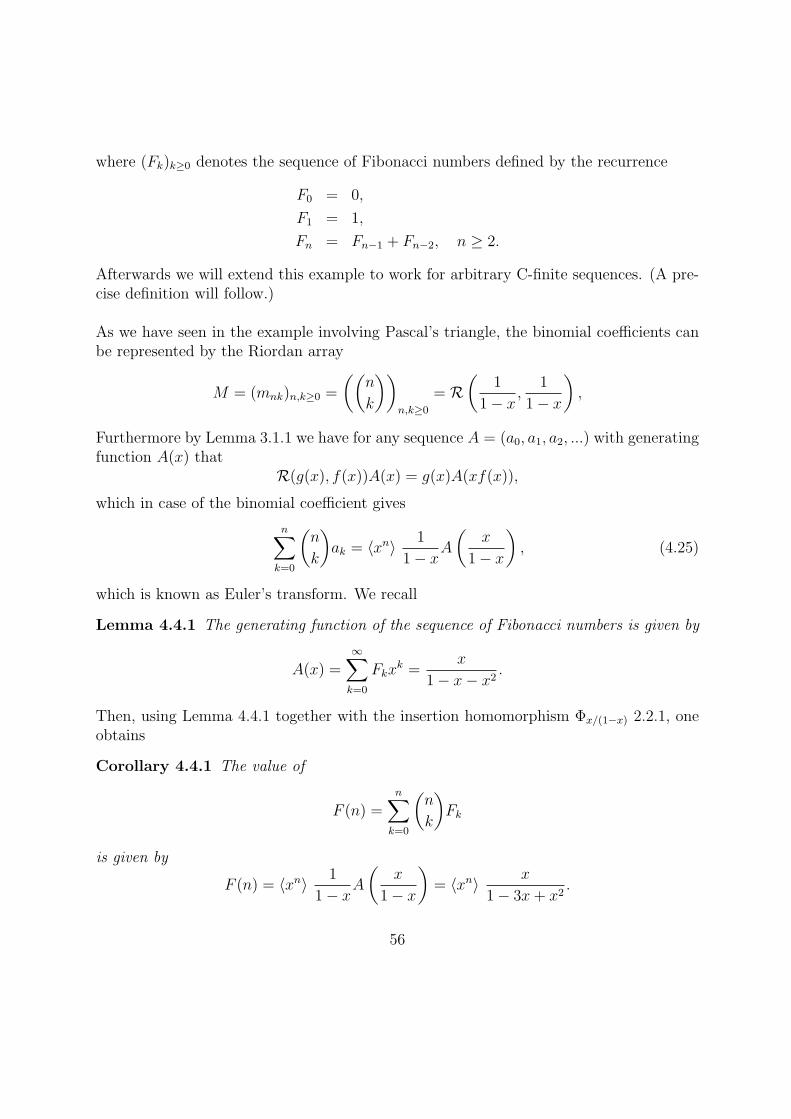
where (Fk)k≥0 denotes the sequence of Fibonacci numbers defined by the recurrence
F0 = 0,
F1 = 1,
Fn = Fn−1 + Fn−2, n ≥ 2.
Afterwards we will extend this example to work for arbitrary C-finite sequences. (A pre-cise definition will follow.)
As we have seen in the example involving Pascal’s triangle, the binomial coefficients canbe represented by the Riordan array
M = (mnk)n,k≥0 =
((n
k
))n,k≥0
= R(
1
1− x,
1
1− x
),
Furthermore by Lemma 3.1.1 we have for any sequence A = (a0, a1, a2, ...) with generatingfunction A(x) that
R(g(x), f(x))A(x) = g(x)A(xf(x)),
which in case of the binomial coefficient gives
n∑k=0
(n
k
)ak = ⟨xn⟩ 1
1− xA
(x
1− x
), (4.25)
which is known as Euler’s transform. We recall
Lemma 4.4.1 The generating function of the sequence of Fibonacci numbers is given by
A(x) =∞∑k=0
Fkxk =
x
1− x− x2.
Then, using Lemma 4.4.1 together with the insertion homomorphism Φx/(1−x) 2.2.1, oneobtains
Corollary 4.4.1 The value of
F (n) =n∑
k=0
(n
k
)Fk
is given by
F (n) = ⟨xn⟩ 1
1− xA
(x
1− x
)= ⟨xn⟩ x
1− 3x+ x2.
56
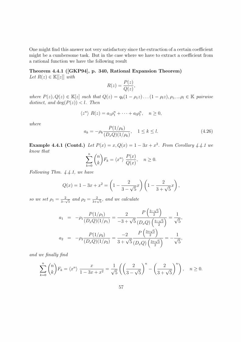
One might find this answer not very satisfactory since the extraction of a certain coefficientmight be a cumbersome task. But in the case where we have to extract a coefficient froma rational function we have the following result
Theorem 4.4.1 ([GKP94], p. 340, Rational Expansion Theorem)Let R(z) ∈ K[[z]] with
R(z) =P (z)
Q(z),
where P (z), Q(z) ∈ K[z] such that Q(z) = q0(1 − ρ1z) . . . (1 − ρlz), ρ1, ...ρl ∈ K pairwisedistinct, and deg(P (z)) < l. Then
⟨zn⟩ R(z) = a1ρn1 + · · ·+ alρ
nl , n ≥ 0,
where
ak = −ρkP (1/ρk)
(DxQ)(1/ρk), 1 ≤ k ≤ l. (4.26)
Example 4.4.1 (Contd.) Let P (x) = x,Q(x) = 1− 3x + x2. From Corollary 4.4.1 weknow that
n∑k=0
(n
k
)Fk = ⟨xn⟩ P (x)
Q(x), n ≥ 0.
Following Thm. 4.4.1, we have
Q(x) = 1− 3x+ x2 =
(1− 2
3−√5x
)(1− 2
3 +√5x
),
so we set ρ1 =2
3−√5and ρ2 =
23+
√5, and we calculate
a1 = −ρ1P (1/ρ1)
(DxQ)(1/ρ1)=
2
−3 +√5
P(
3−√5
2
)(DxQ)
(3−
√5
2
) =1√5,
a2 = −ρ2P (1/ρ2)
(DxQ)(1/ρ2)=
−2
3 +√5
P(
3+√5
2
)(DxQ)
(3+
√5
2
) = − 1√5,
and we finally find
n∑k=0
(n
k
)Fk = ⟨xn⟩ x
1− 3x+ x2=
1√5
((2
3−√5
)n
−(
2
3 +√5
)n), n ≥ 0.
57
Proof. [Proof of Thm. 4.4.1, see [GKP94]]
Let a1, ..., al be as defined in (4.26). Formula (4.26) holds if R(z) = P (z)/Q(z) is equalto
S(z) =a1
1− ρ1z+ · · ·+ al
1− ρlz.
And we can prove that R(z) = S(z) by showing that the function T (z) = R(z) − S(z)is not infinite as z → 1/ρk for all k ∈ {1, . . . , l}. For this will show that the rationalfunction T (z) is never infinite; hence T (z) must be a polynomial. We also can show thatT (z) → 0 as z → ∞; hence T (z) must be zero.
Let αk = 1/ρk. To prove thatlimz→αk
T (z) = ∞,
it suffices to show that limz→αk(z−αk)T (z) = 0, because T (z) is a rational function of z.
Thus we want to show that
limz→αk
(z − αk)R(z) = limz→αk
(z − αk)S(z).
The right-hand limit equals limz→αkak(z − αk)/(1− ρkz) = −ak/ρk, because (1− ρkz) =
−ρk(z − αk) and (z − αk)/(1− ρjz) → 0 for j = k. The left-hand limit is
limz→αk
(z − αk)P (z)
Q(z)= P (αk) lim
z→ak
z − αk
Q(z)=
P (αk)
(DxQ)(αk),
by l’Hospital’s rule. Thus the theorem is proved.2
In general the roots of a polynomial are not distinct. For the case that we have got a rootof multiplicity > 1, we use the following theorem.
Theorem 4.4.2 ((General Version), [GKP94], p. 341)Let R(z) ∈ K[[z]] with
R(z) =P (z)
Q(z),
where P (z), Q(z) ∈ K[z]such that Q(z) = q0(1−ρ1z)d1 . . . (1−ρlz)
dl , ρ1, ..., ρl ∈ K pairwisedistinct, d1, ..., dl ∈ N\{0} and deg(P (z)) < l. Then
⟨zn⟩ R(z) = f1(n)ρn1 + · · ·+ fl(n)ρ
nl , n ≥ 0,
where each fk(n) is a polynomial of degree dk − 1 with leading coefficient
ak = (−ρk)dk
P (1/ρk)dk
(Ddkx Q)(1/ρk)
=P (1/ρk)
(dk − 1)!q0∏
j =k(1− ρj/ρk)dj. (4.27)
58
Example 4.4.2 Consider
rat(x) :=3x4 + 2x3 + x2 + 1
−4 + 4x+ 7x2 − 6x3 − 4x4 + 2x5 + x6
We compute
−4 + 4x+ 7x2 − 6x3 − 4x4 + 2x5 + x6 = −4(1 +
x
2
)2(1− x)3(1 + x),
and hence q0 = −4, ρ1 = −12, d1 = 2, ρ2 = 1, d2 = 3, ρ3 = −1, d3 = 1. The numbers ρi are
pairwise distinct, deg(P (z)) = 4 < d1 + d2 + d3 = 6. We compute the coefficients ak byformula (4.27). By the theorem we get
⟨xn⟩ rat(x) =(
37
108n+ c1
)(−2)−n +
(− 7
36n2 + c2n+ c3
)− 3
8(−1)n︸ ︷︷ ︸
fn
This gives us an Ansatz for the general shape of our expression. If we now compute thefirst 3 values (corresponding to 3 unknowns) of the Taylor expansion we get
3x4 + 2x3 + x2 + 1
−4 + 4x+ 7x2 − 6x3 − 4x4 + 2x5 + x6= −1
4− 1
4x− 15
16x2 +O(x3),
and we can read off f0 = f1 = −1/4 and f2 = −15/16. Equipped with this additionalinformation we can now set up a linear system of equations
1 0 1
−1/2 1 1
1/4 2 1
c1
c2
c3
=
1/8
−7/27
19/432
that has the unique solution (11/36, 2/27,−13/72)T . Hence, we find that
⟨xn⟩ rat(x) =(
37
108n+
11
36
)(−2)−n +
(− 7
36n2 +
2
27n− 13
72
)− 3
8(−1)n.
Example 4.4.3 (Application: non-congruent triangles)In [APR01] the following application is described: What is the number of non-congruenttriangles with prescribed perimeter n ∈ N \{0} and sides a, b, c of positive integer length?The triangles are described via the conditions on the sides
n = a+ b+ c,
1 ≤ a ≤ b ≤ c,
59
and the conditions that we are examining triangles, i.e. the triangle inequalities:
a ≥ b+ c,
b ≥ a+ c,
c ≥ a+ b.
If Tn denotes the number of such tuples, then it is derived in [APR01] that the generatingfunction is given by
∞∑n=0
Tnxn =
x3
(1− x2)(1− x3)(1− x4)= x3 + x5 + x6 + 2x7 + x8 + 3x9 + . . . (4.28)
If we apply the theorem we get the explicit formula
Tk =1
48
(16
3
(− 1
2+ i
√3
2
)k
− (3 + 3i)(−i)k − (3− 3i)(i)k +1
6
(1
2+ i
√3
2
)·(8− 8
(1
2+ i
√3
2
)+ 9
(− 1
2+ i
√3
2
))+
16
3
(− 1
2− i
√3
2
)k
+1
3
(1 + 8
(1
2+ i
√3
2
)−8
(− 1
2+ i
√3
2
))k + k2 − 3(−1)k
(1
18
(19 + 8
(1
2+ i
√3
2
)− 8
(− 1
2+ i
√3
2
)+ k
)),
where i2 = −1, or after further simplification (i.e. rewriting complex numbers to trigono-metric functions)
Tk =1
288
(− 1 + 6k(3 + k)− 36 cos
(kπ
2
)+ 64 cos
(2kπ
3
)− 9(3 + 2k) cos(kπ)
−36 sin
(kπ
2
)− 9i(3 + 2k) sin(kπ)︸ ︷︷ ︸
=0
), k ≥ 0.
Note: The trigonometric functions are coding periodicity, e.g., cos(kπ) = (−1)k.
The general case
Definition 4.4.1 (C-Finite sequence) Let α1, α2, ..., αd be elements in K, d ≥ 1, andαd = 0. The sequence (fn)n≥0 is C-finite if and only if
fn+d + α1fn+d−1 + α2fn+d−2 + · · ·+ αdfn = 0, n ≥ 0.
We will abbreviate the set of C-finite sequences by CF, i.e.,
CF := {(f0, f1, ...) ∈ KN | ∃ (α1, ..., αd) ∈ Kd, αd = 0
∀n ≥ 0 : fn+d + α1fn+d−1 + · · ·+ αdfn = 0}
60
The sequence of Fibonacci numbers (Fk)k≥0 is ∈ CF by the choice α1 = α2 = −1. C-finite sequences have the nice property that their generating function can be expressed arational function. In particular we have the following theorem:
Theorem 4.4.3 ([Sta86], p. 202, [KP11], p. 74) Let α1, α2, ..., αd be elements in K,d ≥ 1 and αd = 0. The following conditions on a function f : N → K are equivalent:
• ∑n≥0
fnxn =
P (x)
Q(x)
where Q(x) = 1 + α1x+ α2x2 + · · ·+ αdx
d ∈ K[x] and P (x) ∈ K[x] is a polynomialin x of degree less than d.
• For all n ≥ 0,fn+d + α1fn+d−1 + α2fn+d−2 + · · ·+ αdfn = 0.
• For all n ≥ 0,
fn =k∑
i=1
Pi(n)γni
where
1 + α1x+ α2x2 + · · ·+ αdx
d =k∏
i=1
(1− γix)di
and the γi’s are distinct elements in K, the algebraic closure of K, and the Pi(x) arepolynomials in K[x] of degree less than di.
Proof. See [Sta86, p. 203] 2
Theorem 4.4.4 Let (Ck)k≥0 ∈ CF. Then:
∞∑n=0
xn
(n∑
k=0
(n
k
)Ck
)
is a rational function.
Proof. The binomial coefficients correspond to the Riordan array
D = R(
1
1− x,
1
1− x
)
61
and hence, by (4.25) we find that
∞∑n=0
xn
(n∑
k=0
(n
k
)Ck
)=
1
1− xC
(x
1− x
)where C(x) ∈ K[[x]] is the generating function of the sequence (Ck)k≥0. Because of theassumption that (Ck)k≥0 ∈ CF we know that C(x) is a rational function. Compositionof C(x) by x/(1− x) and multiplication by 1/(1− x) is again a rational function. 2
Theorem 4.4.5 Let (Ck)k≥0 ∈ CF.
• If a, b ∈ N such that 1 ≤ b ≤ a+ 1:
∞∑n=0
xn
(n∑
k=0
(m+ n+ ak
m+ bk
)Ck
)∈ K(x).
• If a ∈ N, b ∈ Z such that −1 ≤ b ≤ a− 1:
∞∑m=0
xm
(m∑k=0
(n+ ak
m+ bk
)Ck
)∈ K(x).
Proof. The proof proceeds with the same steps as the proof of the previous theorem. Ifwe take n ∈ N fixed and consider
⟨xn⟩ 1
(1− x)m+1
(xb−a
(1− x)b
)k
= ⟨xn⟩ xbk−ak
(1− x)m+1+bk
= ⟨xn−bk+ak⟩ (1− x)−m−1−bk
= (−1)n−bk+ak
(−m− 1− bk
n− bk + ak
)=
(m+ n+ ak
n− bk + ak
)=
(m+ n+ ak
m+ bk
), m, k ≥ 0.
Similar, for m ∈ N fixed:
⟨xm⟩ (1 + x)n(
x−b
(1 + x)−a
)k
= ⟨xm⟩ (1 + x)nxkb
(1 + x)−ka
= ⟨xm+kb⟩ (1 + x)n+ak
=
(n+ ak
m+ bk
), n, k ≥ 0.
62
This suggests to consider the Riordan arrays((m+ n+ ak
m+ bk
))n,k≥0
= R(
1
(1− x)m+1,xb−a−1
(1− x)b
)((
n+ ak
m+ bk
))m,k≥0
= R((1 + x)n,
x−b−1
(1 + x)−a
).
To prove that this are indeed Riordan arrays, we convince ourselves (by standard manip-ulations as above), that by the assumptions on a, b ∈ Z all formal power series involvedhave non-zero constant term.
⟨x0⟩ 1
(1− x)m+1= 1 = 0,
⟨x0⟩ xb−a−1
(1− x)b=
(a
b− 1
)= 0,
⟨x0⟩(1 + x)n = 1 = 0,
⟨x0⟩ x−b−1
(1 + x)−a=
(a
b+ 1
)= 0.
We find by (3.7) for a, b ∈ N such that 1 ≤ b ≤ a+ 1:
∞∑n=0
xn
(n∑
k=0
(m+ n+ ak
m+ bk
)Ck
)=
1
(1− x)m+1C
(xb−a
(1− x)b
), (4.29)
resp. for a ∈ N, b ∈ Z such that −1 ≤ b ≤ a− 1:
∞∑m=0
xm
(m∑k=0
(n+ ak
m+ bk
)Ck
)= (1 + x)nC(x−b(1 + x)a). (4.30)
Again we take into account that composition and multiplication by rational functionskeeps the sum in the field of rational functions. 2
In Connection with Thm. 4.4.2 we can always compute symbolically the value of
{n,m}∑k=0
(n+ ak
m+ bk
)Ck,
for any (Ck)k≥0 ∈ CF and an appropriate choice of m,n ∈ N, in the way illustrated above.
63
Noteworthy is also that, by Thm. 4.4.3, the sequence
(A{m,n}
){m,n}≥0
=
{m,n}∑k=0
(n+ ak
m+ bk
)Ck
{m,n}≥0
,
with (Ck)k≥0 ∈ CF, also satisfies a C-finite recurrence.
Example 4.4.4 ([Wil06], p.162, Ex. 4.16)If two sequences (fn)n≥0 and (ck)k≥0 are connected by the equations
fn =∑k
(n+ k
m+ 2k
)ck, n ≥ 0,
where m ≥ 0 is fixed, then their opsgf ’s are connected by
F (x) =xm
(1− x)m+1C
(x
(1− x)2
)Proof. Let
F (x) =∞∑n=0
fnxn, C(x) =
∞∑n=0
cnxn.
Then
⟨xn⟩F (x) = fn =∑k
(n+ k
m+ 2k
)ck =
n−m∑k=0
(n+ k
m+ 2k
)ck,
because of the ”support” of the binomial coefficient. By (4.29) we have that
⟨xn⟩ xm
(1− x)m+1C
(x
(1− x)2
)= ⟨xn−m⟩ 1
(1− x)m+1C
(x2−1
(1− x)2
)=
n−m∑k=0
(n+ k
m+ 2k
)ck.
Note that the sequence (ck)k≥0 does not has to be necessarily in CF. This restrictionallows us to compute the value in a symbolical fashion (because then we have a rationalgenerating function) but has not to be necessarily the case. 2
64
As we have seen in this discussion the case where the sequence of coefficients satisfy aC-finite recurrence can always be fully solved. In particular we can always give an explicitformula for the general term ck.
The author was pointed to the work of Koutschan [Kou09, Kou10] who examined ap-plications of the holonomic systems approach. He developed the Mathematica packageHolonomicFunctions which computes the annihilator of the sum
∑nk=0
(nk
)Fk. We will
present how to proceed in Mathematica.
Mathematica 7.0 - Listing
In[1]:= <<HolonomicFunctions.mHolonomicFunctions package by Christoph Koutschan, RISC-Linz, Version 1.3 (25.01.2010)
In[2]:= Annihilator[Sum[Binomial[n, k] ∗ Fibonacci[k], {k, 0, n}], S[n]]
Out[2]= {S2n − 3Sn + 1}
Hence, if we denote F (n) =∑n
k=0
(nk
)Fk we know from this that
F (n+ 2)− 3F (n+ 1) + F (n) = 0
holds for n ≥ 0. If we compute initial values we can invoke Thm. 4.4.3 to compute aclosed form for the sum in question.
4.5 An explicit formula for Stirling numbers
From the combinatorial interpretation of Stirling numbers of the second kind, one find arecurrence relation for these numbers. The Stirling numbers of the second kind satisfythe recurrence [Wil06, p. 17]
S2(n, k) = S2(n− 1, k − 1) + kS2(n− 1, k). (4.31)
Proof. Take a set with n elements and highlight one particular element, say for instancethe last one. To obtain a partition of the n element set into k blocks we can partition then−1 element set (where we excluded our highlighted element) into k blocks and place thelast element into any of these blocks in kS2(n− 1, k) ways, or we can put the last elementin a block by itself and partition the n−1 element set into k−1 blocks in S2(n−1, k−1)ways. So the total number of ways is given by (4.31)
2
65
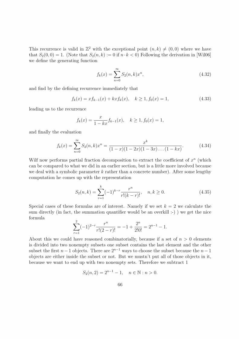
This recurrence is valid in Z2 with the exceptional point (n, k) = (0, 0) where we havethat S2(0, 0) = 1. (Note that S2(n, k) := 0 if n ·k < 0) Following the derivation in [Wil06]we define the generating function
fk(x) =∞∑n=0
S2(n, k)xn, (4.32)
and find by the defining recurrence immediately that
fk(x) = xfk−1(x) + kxfk(x), k ≥ 1, f0(x) = 1, (4.33)
leading us to the recurrence
fk(x) =x
1− kxfk−1(x), k ≥ 1, f0(x) = 1,
and finally the evaluation
fk(x) =∞∑n=0
S2(n, k)xn =
xk
(1− x)(1− 2x)(1− 3x) . . . (1− kx). (4.34)
Wilf now performs partial fraction decomposition to extract the coefficient of xn (whichcan be compared to what we did in an earlier section, but is a little more involved becausewe deal with a symbolic parameter k rather than a concrete number). After some lengthycomputation he comes up with the representation
S2(n, k) =k∑
r=1
(−1)k−r rn
r!(k − r)!, n, k ≥ 0. (4.35)
Special cases of these formulas are of interest. Namely if we set k = 2 we calculate thesum directly (in fact, the summation quantifier would be an overkill :-) ) we get the niceformula
2∑r=1
(−1)2−r rn
r!(2− r)!= −1 +
2n
2!0!= 2n−1 − 1.
About this we could have reasoned combinatorially, because if a set of n > 0 elementsis divided into two nonempty subsets one subset contains the last element and the othersubset the first n− 1 objects. There are 2n−1 ways to choose the subset because the n− 1objects are either inside the subset or not. But we mustn’t put all of those objects in it,because we want to end up with two nonempty sets. Therefore we subtract 1
S2(n, 2) = 2n−1 − 1, n ∈ N : n > 0.
66
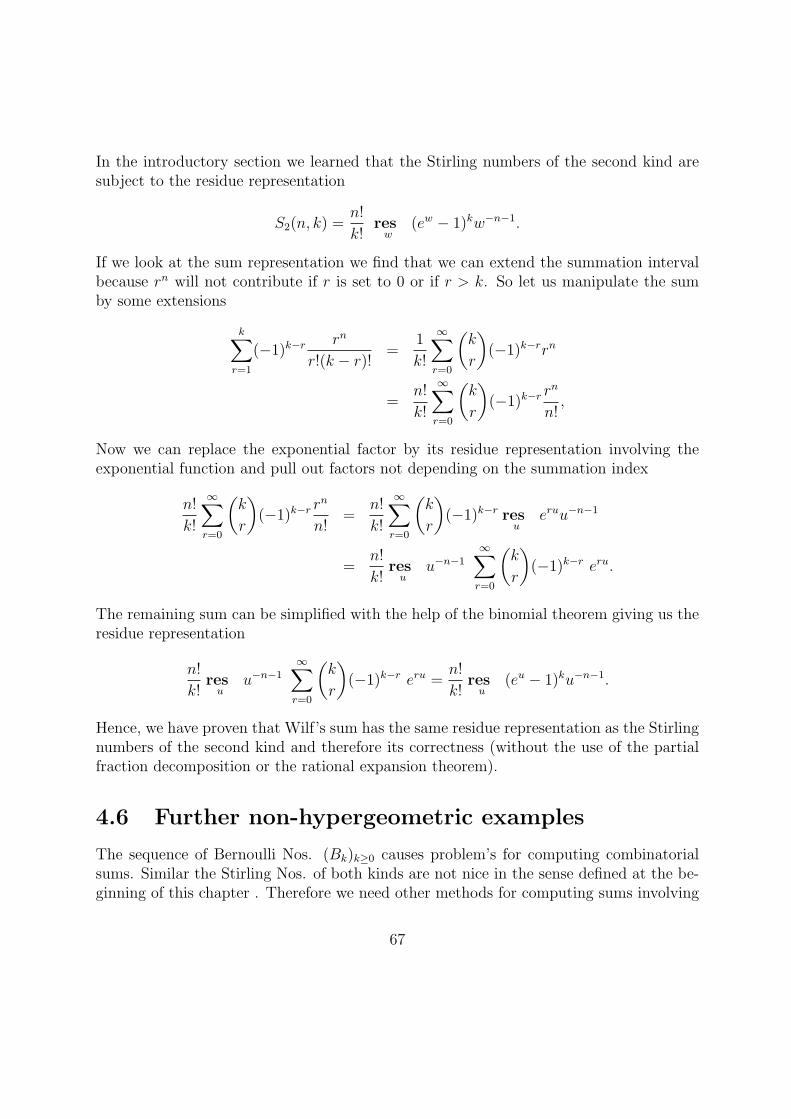
In the introductory section we learned that the Stirling numbers of the second kind aresubject to the residue representation
S2(n, k) =n!
k!resw
(ew − 1)kw−n−1.
If we look at the sum representation we find that we can extend the summation intervalbecause rn will not contribute if r is set to 0 or if r > k. So let us manipulate the sumby some extensions
k∑r=1
(−1)k−r rn
r!(k − r)!=
1
k!
∞∑r=0
(k
r
)(−1)k−rrn
=n!
k!
∞∑r=0
(k
r
)(−1)k−r r
n
n!,
Now we can replace the exponential factor by its residue representation involving theexponential function and pull out factors not depending on the summation index
n!
k!
∞∑r=0
(k
r
)(−1)k−r r
n
n!=
n!
k!
∞∑r=0
(k
r
)(−1)k−r res
ueruu−n−1
=n!
k!res
uu−n−1
∞∑r=0
(k
r
)(−1)k−r eru.
The remaining sum can be simplified with the help of the binomial theorem giving us theresidue representation
n!
k!res
uu−n−1
∞∑r=0
(k
r
)(−1)k−r eru =
n!
k!res
u(eu − 1)ku−n−1.
Hence, we have proven that Wilf’s sum has the same residue representation as the Stirlingnumbers of the second kind and therefore its correctness (without the use of the partialfraction decomposition or the rational expansion theorem).
4.6 Further non-hypergeometric examples
The sequence of Bernoulli Nos. (Bk)k≥0 causes problem’s for computing combinatorialsums. Similar the Stirling Nos. of both kinds are not nice in the sense defined at the be-ginning of this chapter . Therefore we need other methods for computing sums involving
67
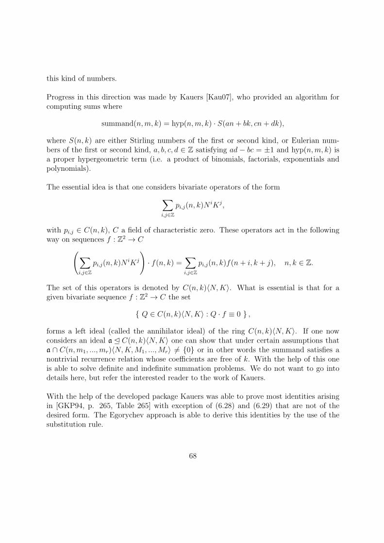
this kind of numbers.
Progress in this direction was made by Kauers [Kau07], who provided an algorithm forcomputing sums where
summand(n,m, k) = hyp(n,m, k) · S(an+ bk, cn+ dk),
where S(n, k) are either Stirling numbers of the first or second kind, or Eulerian num-bers of the first or second kind, a, b, c, d ∈ Z satisfying ad − bc = ±1 and hyp(n,m, k) isa proper hypergeometric term (i.e. a product of binomials, factorials, exponentials andpolynomials).
The essential idea is that one considers bivariate operators of the form∑i,j∈Z
pi,j(n, k)NiKj,
with pi,j ∈ C(n, k), C a field of characteristic zero. These operators act in the followingway on sequences f : Z2 → C(∑
i,j∈Z
pi,j(n, k)NiKj
)· f(n, k) =
∑i,j∈Z
pi,j(n, k)f(n+ i, k + j), n, k ∈ Z.
The set of this operators is denoted by C(n, k)⟨N,K⟩. What is essential is that for agiven bivariate sequence f : Z2 → C the set
{ Q ∈ C(n, k)⟨N,K⟩ : Q · f ≡ 0 } ,
forms a left ideal (called the annihilator ideal) of the ring C(n, k)⟨N,K⟩. If one nowconsiders an ideal a � C(n, k)⟨N,K⟩ one can show that under certain assumptions thata ∩ C(n,m1, ...,mr)⟨N,K,M1, ...,Mr⟩ = {0} or in other words the summand satisfies anontrivial recurrence relation whose coefficients are free of k. With the help of this oneis able to solve definite and indefinite summation problems. We do not want to go intodetails here, but refer the interested reader to the work of Kauers.
With the help of the developed package Kauers was able to prove most identities arisingin [GKP94, p. 265, Table 265] with exception of (6.28) and (6.29) that are not of thedesired form. The Egorychev approach is able to derive this identities by the use of thesubstitution rule.
68
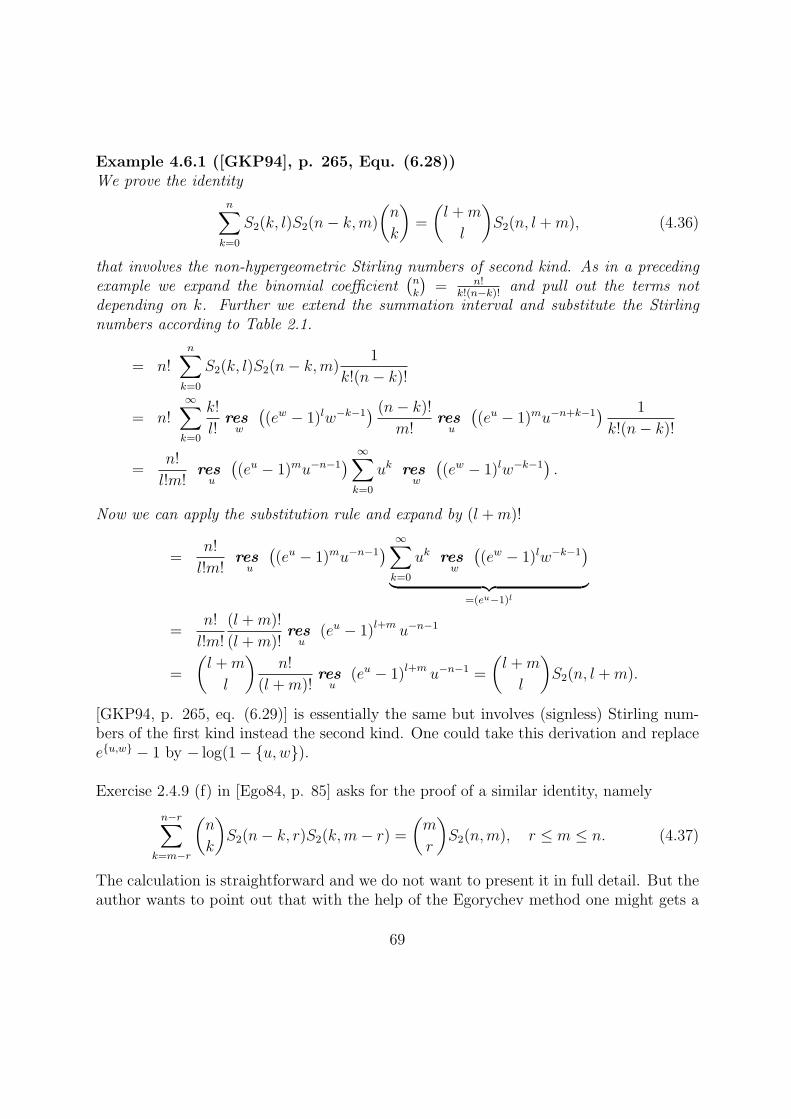
Example 4.6.1 ([GKP94], p. 265, Equ. (6.28))We prove the identity
n∑k=0
S2(k, l)S2(n− k,m)
(n
k
)=
(l +m
l
)S2(n, l +m), (4.36)
that involves the non-hypergeometric Stirling numbers of second kind. As in a precedingexample we expand the binomial coefficient
(nk
)= n!
k!(n−k)!and pull out the terms not
depending on k. Further we extend the summation interval and substitute the Stirlingnumbers according to Table 2.1.
= n!n∑
k=0
S2(k, l)S2(n− k,m)1
k!(n− k)!
= n!∞∑k=0
k!
l!res
w
((ew − 1)lw−k−1
) (n− k)!
m!res
u
((eu − 1)mu−n+k−1
) 1
k!(n− k)!
=n!
l!m!res
u
((eu − 1)mu−n−1
) ∞∑k=0
uk resw
((ew − 1)lw−k−1
).
Now we can apply the substitution rule and expand by (l +m)!
=n!
l!m!res
u
((eu − 1)mu−n−1
) ∞∑k=0
uk resw
((ew − 1)lw−k−1
)︸ ︷︷ ︸
=(eu−1)l
=n!
l!m!
(l +m)!
(l +m)!res
u(eu − 1)l+m u−n−1
=
(l +m
l
)n!
(l +m)!res
u(eu − 1)l+m u−n−1 =
(l +m
l
)S2(n, l +m).
[GKP94, p. 265, eq. (6.29)] is essentially the same but involves (signless) Stirling num-bers of the first kind instead the second kind. One could take this derivation and replacee{u,w} − 1 by − log(1− {u,w}).
Exercise 2.4.9 (f) in [Ego84, p. 85] asks for the proof of a similar identity, namely
n−r∑k=m−r
(n
k
)S2(n− k, r)S2(k,m− r) =
(m
r
)S2(n,m), r ≤ m ≤ n. (4.37)
The calculation is straightforward and we do not want to present it in full detail. But theauthor wants to point out that with the help of the Egorychev method one might gets a
69
handle on a more general class than what Kauers calls a proper Stirling-like term.
For handling Stirling Number identities, it is pointed out in [Spr94] that the Riordanarray approach is also applicable.
Lemma 4.6.1 For k ∈ N fixed:
(− log (1− x))k = k!∞∑n=0
S1(n, k)xn
n!, (4.38)
(ex − 1)k = k!∞∑n=0
S2(n, k)xn
n!. (4.39)
Let us consider the Riordan array
M := (mn,k), where mn,k := S1(n, k)k!
n!.
Then, the Riordan matrix M will look like M = (M (0),M (1),M (2), ...), where
M (0) =
1
0
0...
= first column of M , (4.40)
and
M (k) =
S1(0, k)
k!0!
S1(1, k)k!1!
S1(2, k)k!2!
...
= kth column of M , (4.41)
By Lemma 4.6.1, the generating function of the kth column is given by (− log(1 − x))k.We can reason similar for the Stirling numbers of the second kind, and hence we havefound the Riordan arrays(
S1(n, k)k!
n!
)n,k≥0
= R(1,−1
xlog (1− x)
), (4.42)(
S2(n, k)k!
n!
)n,k≥0
= R(1,
1
x(ex − 1)
). (4.43)
To see how easy this will work with Riordan arrays we will illustratively show an example.
70
Example 4.6.2 ([Spr94])
n∑k=0
S2(n, k)k!(−1)k
k + 1= Bn (4.44)
We start by rewriting the original summand as follows:
n∑k=0
S2(n, k)k!(−1)k
k + 1= n!
n∑k=0
S2(n, k)k!
n!
(−1)k
k + 1(4.45)
As noted above, we can identify by the Stirling numbers of the second kind by the Riordanarray (
S2(n, k)k!
n!
)n,k≥0
= R(g(x), f(x)) = R(1,
1
x(ex − 1)
).
The sequence((−1)k/(k + 1)
)k≥0
has the generating function
∞∑k=0
(−1)k
k + 1xk =
1
x
∞∑k=0
(−1)k
k + 1xk+1 =
1
x
∞∑k=1
(−1)k−1
kxk =
1
x
∞∑k=1
(−1)k+1
kxk =
log(1 + x)
x.
(4.46)Hence, by Lemma 3.1.1 and (2.49) we find that:
B(x) = g(x)A(xf(x)) =log(1 + (ex − 1))
ex − 1=
x
ex − 1
and therefore
n!n∑
k=0
S2(n, k)k!
n!
(−1)k
k + 1= n! ⟨xn⟩ x
ex − 1= Bn.
where the last step is a consequence from (2.53).
4.7 Symbolic Sums involving holonomic sequences
As we have seen in the last section, we sometimes might have to extract the coefficient of xn
of a generating function that is not rational. In particular in examples involving Stirlingnumbers we might get generating functions that contain logarithmic resp. exponentialfactors. In this case we know by Thm. 4.4.3 that the coefficients will not satisfy a C-finiterecurrence. We start again by a concrete example and generalize afterwards.
71
Example 4.7.1 Suppose we want to extract
⟨xn⟩ f(x) := x− log(1 + x) + x log(1 + x)
x2.
Again we take Mallinger’s package in action to obtain information about the behaviourof the sequence. For this purpose we start by computing the first 10 values of the Taylorexpansion of the series.
Mathematica 7.0 - Listing
In[1]:= CoefficientList
[Series
[x − Log[1 + x] + xLog[1 + x]
x2, {x, 0, 15}
], x
]
Out[1]=
{3
2,−
5
6,7
12,−
9
20,11
30,−
13
42,15
56,−
17
72,19
90,−
21
110,23
132
}
No obvious pattern is visible from the coefficient list. We have to work a little more to geta closed form for general fn. If we try Mallinger’s procedures we might obtain a recurrencerelation with polynomial coefficients:
Mathematica 7.0 - Listing
In[2]:= GuessRE
[{3
2,−
5
6,
7
12,−
9
20,11
30,−
13
42,15
56,−
17
72,19
90,−
21
110,
23
132
}, a [n]
]
Out[2]=
{{(−1− n)a[n] + a[1 + n] + (4 + n)a[2 + n] == 0, a[0] ==
3
2, a[1] == −
5
6
}, ”ogf”
}
The initial values are actually no surprise. But the author of this work guesses from thelist of coefficients no person would have come up with this recurrence relation.
How to solve this recurrence equation? There is a built in Mathematica function that canhandle C-finite recurrences and also recurrences of this type. Indeed, if one tries
Mathematica 7.0 - Listing
In[3]:= RSolve
[{(−1 − n)a[n] + a[1 + n] + (4 + n)a[2 + n] == 0, a[0] ==
3
2, a[1] == −
5
6
}, a[n], n
]
Out[3]=
{{a[n] →
(−1)n(3 + 2n)
(n2 + 3n+ 2)
}}
72
one gets already a closed form for the general term. An alternative is to apply Petkovsek’salgorithm Hyper (see [Pet98] and [PWZ96]) for finding hypergeometric solutions to suchequations (we will come back to this).
The general caseIn general it will be the case that the order of the guessed recurrence for the coefficientsequence will be higher than 2. Let us develop the theory for higher order equations.
Definition 4.7.1 (See [Mal96], p. 10, Def. 1.3.1)A sequence (an)n≥0 ∈ KN is holonomic (or P-recursive) if and only if (an)n≥0 satisfies alinear recurrence with polynomial coefficients (holonomic recurrence equation), i.e., thereare polynomials p0, p1, ..., pd ∈ K[x], pd = 0, such that for all n ∈ N :
p0(n)an + p1(n)an+1 + · · ·+ pd(n)an+d = 0 (4.47)
We will call d the order and max(deg(p0(n), ..., pd(n))) the degree of the recurrence.
Similar as before we denote the set of holonomic sequences by PF standing for P-finite.
As it turns out such recurrences does not only appear here but also in cases of definite andindefinite hypergeometric summation (as in Zeilberger’s creative telescoping respectivelyin Gosper’s algorithm). Therefore mathematicians started to investigate the problem offinding solutions to this kind of equations. We distinguish 3 kind of solutions.
Definition 4.7.2 A sequence (an)n≥0 will be called
• polynomial over K if there is a polynomial f(x) ∈ K[x] such that an = f(n) for alln ∈ N large enough
• rational over K if there is a rational function f(x) ∈ K(x) such that an = f(n) forall n ∈ N large enough
• a hypergeometric term over K if there is a rational function r(x) ∈ K(x) such thatan+1 = r(n)an for all n ∈ N large enough
Petkovsek [Pet98] provides an algorithm not only for finding polynomial solutions but alsofor computing hypergeometric solutions. The algorithm is inspired by Gosper’s algorithm[Gos78] that relies on the fact that any rational function r(x) ∈ K(x) can be representedas
r(x) = ZA(x)
B(x)
C(x+ 1)
C(x)
73
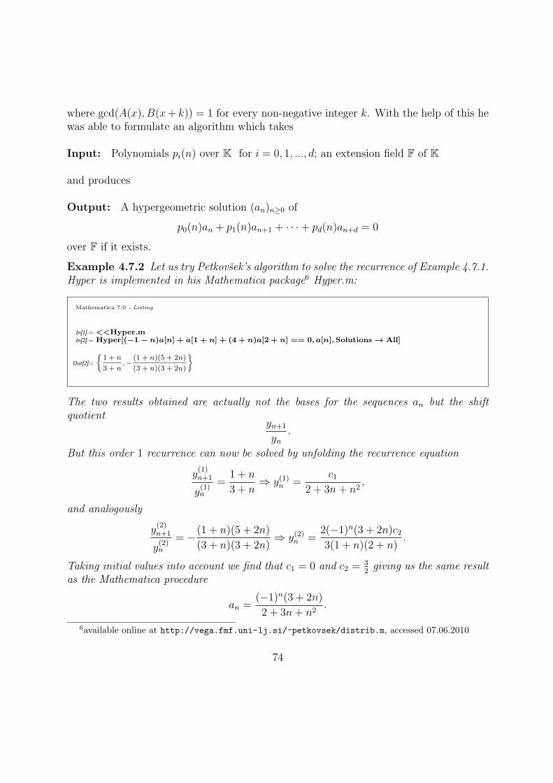
where gcd(A(x), B(x+ k)) = 1 for every non-negative integer k. With the help of this hewas able to formulate an algorithm which takes
Input: Polynomials pi(n) over K for i = 0, 1, ..., d; an extension field F of K
and produces
Output: A hypergeometric solution (an)n≥0 of
p0(n)an + p1(n)an+1 + · · ·+ pd(n)an+d = 0
over F if it exists.
Example 4.7.2 Let us try Petkovsek’s algorithm to solve the recurrence of Example 4.7.1.Hyper is implemented in his Mathematica package6 Hyper.m:
Mathematica 7.0 - Listing
In[1]:= <<Hyper.mIn[2]:= Hyper[(−1 − n)a[n] + a[1 + n] + (4 + n)a[2 + n] == 0, a[n], Solutions → All]
Out[2]=
{1 + n
3 + n,−
(1 + n)(5 + 2n)
(3 + n)(3 + 2n)
}
The two results obtained are actually not the bases for the sequences an but the shiftquotient
yn+1
yn.
But this order 1 recurrence can now be solved by unfolding the recurrence equation
y(1)n+1
y(1)n
=1 + n
3 + n⇒ y(1)n =
c12 + 3n+ n2
,
and analogously
y(2)n+1
y(2)n
= −(1 + n)(5 + 2n)
(3 + n)(3 + 2n)⇒ y(2)n =
2(−1)n(3 + 2n)c23(1 + n)(2 + n)
.
Taking initial values into account we find that c1 = 0 and c2 =32giving us the same result
as the Mathematica procedure
an =(−1)n(3 + 2n)
2 + 3n+ n2.
6available online at http://vega.fmf.uni-lj.si/~petkovsek/distrib.m, accessed 07.06.2010
74
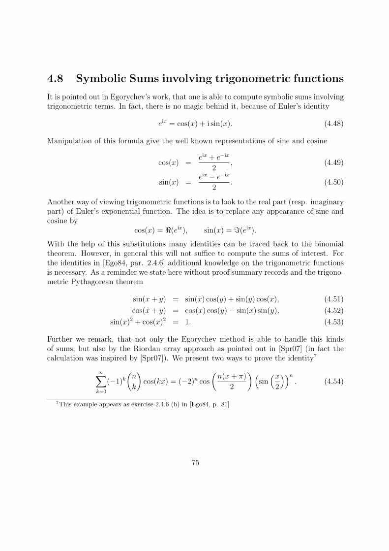
4.8 Symbolic Sums involving trigonometric functions
It is pointed out in Egorychev’s work, that one is able to compute symbolic sums involvingtrigonometric terms. In fact, there is no magic behind it, because of Euler’s identity
eix = cos(x) + i sin(x). (4.48)
Manipulation of this formula give the well known representations of sine and cosine
cos(x) =eix + e−ix
2, (4.49)
sin(x) =eix − e−ix
2. (4.50)
Another way of viewing trigonometric functions is to look to the real part (resp. imaginarypart) of Euler’s exponential function. The idea is to replace any appearance of sine andcosine by
cos(x) = ℜ(eix), sin(x) = ℑ(eix).
With the help of this substitutions many identities can be traced back to the binomialtheorem. However, in general this will not suffice to compute the sums of interest. Forthe identities in [Ego84, par. 2.4.6] additional knowledge on the trigonometric functionsis necessary. As a reminder we state here without proof summary records and the trigono-metric Pythagorean theorem
sin(x+ y) = sin(x) cos(y) + sin(y) cos(x), (4.51)
cos(x+ y) = cos(x) cos(y)− sin(x) sin(y), (4.52)
sin(x)2 + cos(x)2 = 1. (4.53)
Further we remark, that not only the Egorychev method is able to handle this kindsof sums, but also by the Riordan array approach as pointed out in [Spr07] (in fact thecalculation was inspired by [Spr07]). We present two ways to prove the identity7
n∑k=0
(−1)k(n
k
)cos(kx) = (−2)n cos
(n(x+ π)
2
)(sin(x2
))n. (4.54)
7This example appears as exercise 2.4.6 (b) in [Ego84, p. 81]
75
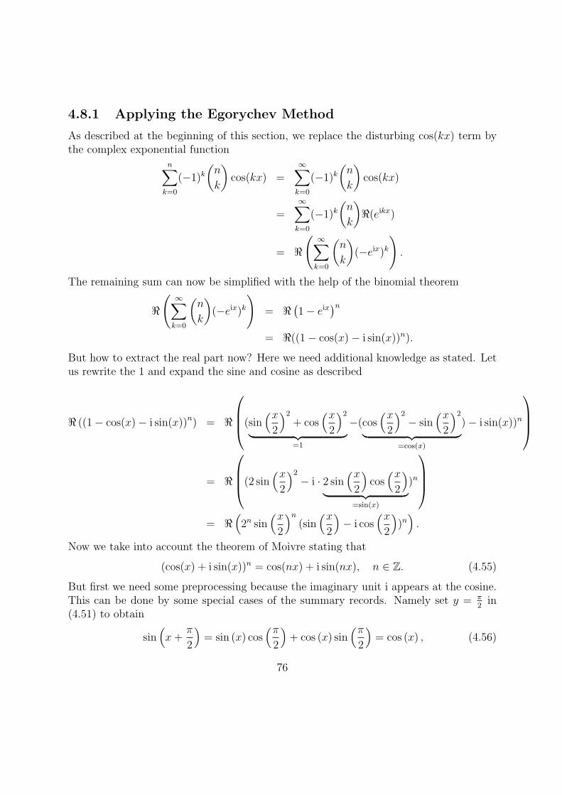
4.8.1 Applying the Egorychev Method
As described at the beginning of this section, we replace the disturbing cos(kx) term bythe complex exponential function
n∑k=0
(−1)k(n
k
)cos(kx) =
∞∑k=0
(−1)k(n
k
)cos(kx)
=∞∑k=0
(−1)k(n
k
)ℜ(eikx)
= ℜ
(∞∑k=0
(n
k
)(−eix)k
).
The remaining sum can now be simplified with the help of the binomial theorem
ℜ
(∞∑k=0
(n
k
)(−eix)k
)= ℜ
(1− eix
)n= ℜ((1− cos(x)− i sin(x))n).
But how to extract the real part now? Here we need additional knowledge as stated. Letus rewrite the 1 and expand the sine and cosine as described
ℜ ((1− cos(x)− i sin(x))n) = ℜ
(sin(x2
)2+ cos
(x2
)2︸ ︷︷ ︸
=1
−(cos(x2
)2− sin
(x2
)2︸ ︷︷ ︸
=cos(x)
)− i sin(x))n
= ℜ
(2 sin(x2
)2− i · 2 sin
(x2
)cos(x2
)︸ ︷︷ ︸
=sin(x)
)n
= ℜ
(2n sin
(x2
)n(sin
(x2
)− i cos
(x2
))n).
Now we take into account the theorem of Moivre stating that
(cos(x) + i sin(x))n = cos(nx) + i sin(nx), n ∈ Z. (4.55)
But first we need some preprocessing because the imaginary unit i appears at the cosine.This can be done by some special cases of the summary records. Namely set y = π
2in
(4.51) to obtain
sin(x+
π
2
)= sin (x) cos
(π2
)+ cos (x) sin
(π2
)= cos (x) , (4.56)
76
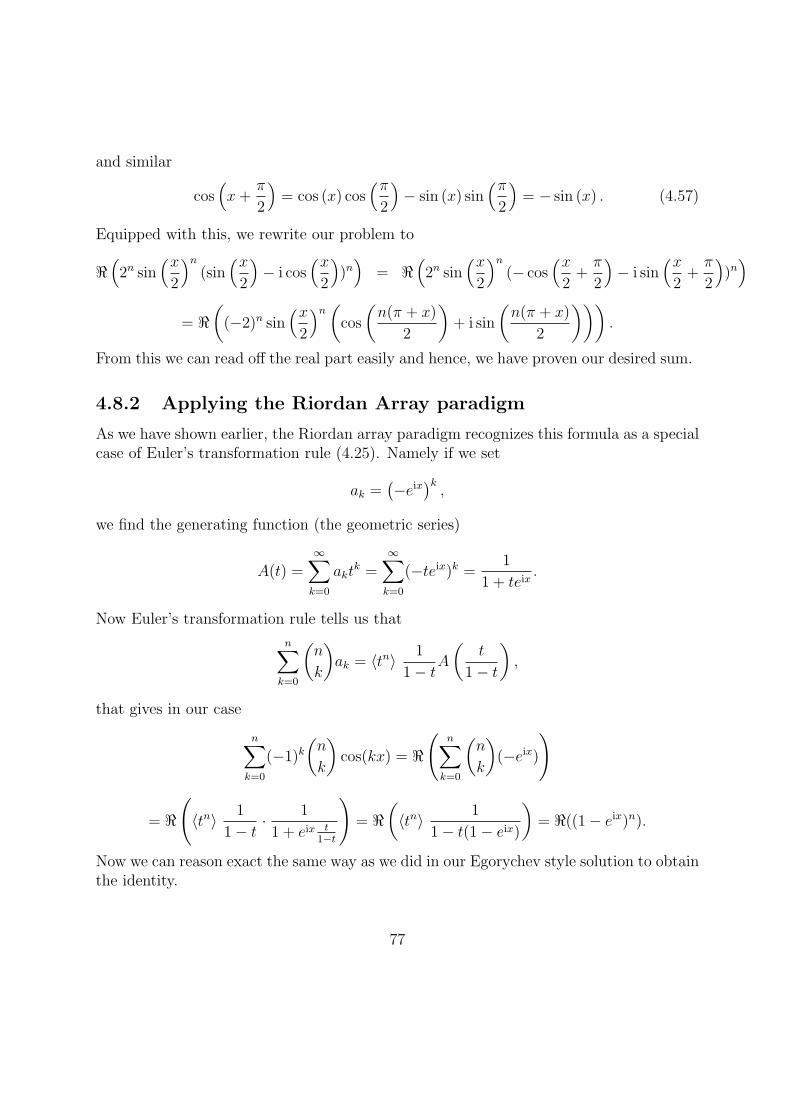
and similar
cos(x+
π
2
)= cos (x) cos
(π2
)− sin (x) sin
(π2
)= − sin (x) . (4.57)
Equipped with this, we rewrite our problem to
ℜ(2n sin
(x2
)n(sin
(x2
)− i cos
(x2
))n)
= ℜ(2n sin
(x2
)n(− cos
(x2+
π
2
)− i sin
(x2+
π
2
))n)
= ℜ((−2)n sin
(x2
)n(cos
(n(π + x)
2
)+ i sin
(n(π + x)
2
))).
From this we can read off the real part easily and hence, we have proven our desired sum.
4.8.2 Applying the Riordan Array paradigm
As we have shown earlier, the Riordan array paradigm recognizes this formula as a specialcase of Euler’s transformation rule (4.25). Namely if we set
ak =(−eix
)k,
we find the generating function (the geometric series)
A(t) =∞∑k=0
aktk =
∞∑k=0
(−teix)k =1
1 + teix.
Now Euler’s transformation rule tells us that
n∑k=0
(n
k
)ak = ⟨tn⟩ 1
1− tA
(t
1− t
),
that gives in our case
n∑k=0
(−1)k(n
k
)cos(kx) = ℜ
(n∑
k=0
(n
k
)(−eix)
)
= ℜ
(⟨tn⟩ 1
1− t· 1
1 + eix t1−t
)= ℜ
(⟨tn⟩ 1
1− t(1− eix)
)= ℜ((1− eix)n).
Now we can reason exact the same way as we did in our Egorychev style solution to obtainthe identity.
77
Remark: Whenever we are able to compute our sum this way we get actually twoidentities. Namely, by considering the imaginary part of our equation we get the identitywith the sine replaced by the cosine for free. In particular we have proven two identities
n∑k=0
(−1)k(n
k
)cos(kx) = (−2)n cos
(n(x+ π)
2
)(sin(x2
))n, n ≥ 0, (4.58)
n∑k=0
(−1)k(n
k
)sin(kx) = (−2)n sin
(n(x+ π)
2
)(sin(x2
))n, n ≥ 0. (4.59)
4.9 An Identity for Jacobi polynomials P(α,β)n (x)
Exercise 4.15 in [Wil06] asks the reader to derive a closed form for the generating func-tion of the Jacobi polynomials. In the following we will show how to make use of theEgorychev and of the Snake Oil method to derive a simple closed form.
The Jacobi polynomials are solutions to the Jacobi differential equation [AAR99, p. 297,(6.3.9)]
(1− x2)y′′(x) + [β − α− (α+ β + 2)x]y′(x) + n(n+ α+ β + 1)y(x) = 0. (4.60)
The first few polynomials are given by
P(α,β)0 (x) = 1
P(α,β)1 (x) =
1
2[2(α+ 1) + (α+ β + 2)(x− 1)]
P(α,β)2 (x) =
1
8[4(α+ 1)(α+ 2) + 4(α+ β + 3)(α+ 2)(x− 1) + (α+ β + 3)(α+ β + 4)(x− 1)2]
A different definition would be over the Rodrigues formula [AAR99, p. 300, Remark 6.4.1]
P (α,β)n (x) =
(1− x)−α(1 + x)−β
(−2)nn!
dn
dxn
[(1− x)n+α(1 + x)n+β
], n ≥ 0. (4.61)
In the following we will give the generating function of Jacobi polynomials. We will derivethat ∑
n
P (α,β)n (x) tn+α+β =
(1 + x− 2t)n+α
2n(x− 1)α(1− t)n+1.
That solves Wilf’s example [Wil06, Ex. 4.1.15, p. 161]. Following Wilf’s proposal, weproceed in 3 steps to show this.
78
Example 4.9.1 ([Wil06], p. 161, Ex. 4.15)For all m,n, q ≥ 0, we have∑
r
(m
r
)(n− r
n− r − q
)(t− 1)r =
∑r
(m
r
)(n−m
n− r − q
)tr.
We will derive a residue representation for both sums in question and show that they arethe same. This proves the claim. Let us first look at the sum at the left hand side.
The convention in Wilf’s book is that the summation index r ranges over the integers. Sothe first step, extending the summation interval precipitates. In the next step we replacethe binomial coefficients by their residue representations∑r
(m
r
)(n− r
n− r − q
)(t− 1)r =
∑r
resw
(1 + w)mw−r−1 resu
(1 + u)n−ru−n+r+q−1 (t− 1)r
= resu
(1 + u)nu−n+q−1∑r
((t− 1)u
(1 + u)
)r
resw
(1 + w)mw−r−1.
Now the substitution rule applies and we find that∑r
(m
r
)(n− r
n− r − q
)(t− 1)r = res
u(1 + u)n−m(1 + ut)mu−n+q−1. (4.62)
For the right hand side start again by replacing the binomial coefficients∑r
(m
r
)(n−m
n− r − q
)tr =
∑r
resw
(1 + w)mw−r−1 resu
(1 + u)n−mu−n+r+q−1tr
= resu
(1 + u)n−mu−n+q−1∑r
(ut)r resw
(1 + w)mw−r−1.
Again, with the help of the substitution rule we find that∑r
(m
r
)(n−m
n− r − q
)tr = res
u(1 + u)n−m(1 + ut)mu−n+q−1. (4.63)
The next step in Wilf’s exercise states that the Jacobi polynomials may be defined forn ≥ 0, by
P (α,β)n (x) =
∑k
(n+ α
k
)(n+ β
n− k
)(x− 1
2
)n−k (x+ 1
2
)k
. (4.64)
79
One should now use the result of part (a) to show also that
P (α,β)n (x) =
∑j
(n+ α+ β + j
j
)(n+ α
j + α
)(x− 1
2
)j
. (4.65)
To see, why this equation holds, we start by considering (4.64) and pulling out constants∑k
(n+ α
k
)(n+ β
n− k
)(x− 1
2
)n−k (x+ 1
2
)k
=
(x− 1
2
)n∑k
(n+ α
k
)(n+ β
n− k
)(x+ 1
x− 1
)k
.
By matching with the sum (4.63) and the assignment of the parameters
m = n+ α,
r = k,
n = 2n+ α+ β,
q = n+ α+ β,
t =x+ 1
x− 1,
we find, with the help of part (a) (observe that t− 1 = 2x−1
), that this sum is equal to(x− 1
2
)n∑k
(n+ α
k
)(n+ β
n− k
)(x+ 1
x− 1
)k
=
(x− 1
2
)n∑k
(n+ α
k
)(2n+ α+ β − k
n− k
)(2
x− 1
)k
=∑k
(n+ α
k
)(n+ α+ β + (n− k)
n− k
)(x− 1
2
)n−k
.
If we now reverse the summation interval (this is replacing k by n−k, a bijective mappingon the summation interval) we get the desired identity
=∑k
(n+ α
n− k
)(n+ α+ β + k
k
)(x− 1
2
)k
=∑j
(n+ α+ β + j
j
)(n+ α
j + α
)(x− 1
2
)j
.
Finally sub exercise (c) wants the reader to use part (b) and a dash of the Snake Oil toshow that
P (α,β)n = 2−n(x− 1)−α ⟨tn+α+β⟩
{(1 + x− 2t)n+α
(1− t)n+1
}. (4.66)
80
To show this, we consider the generating function for Jacobi polynomials
∑n
P (α,β)n (x) tn+α+β =
∑n
tn+α+β
(∑j
(n+ α+ β + j
j
)(n+ α
j + α
)(x− 1
2
)j)
=∑n
(∑j
(n+ α+ β + j
j
)(n+ α
j + α
)(x− 1
2
)j)tn+α+β.
The next step in the Snake Oil method tells to interchange order of summation and replacethe summation variable. Note that we are actually not summing on n but as we shallsee we are summing on n+ α+ β + j. Therefore we can pull out the binomial coefficientalthough it depends on n.
=∑j
(n+ α
j + α
)(x− 1
2t
)j ∑n
(n+ α+ β + j
j
)tn+α+β+j
=∑j
(n+ α
j + α
)(x− 1
2t
)j ∑s
(s
j
)ts.
Hence, together with the elementary generating function∑r
(r
k
)xr =
xk
(1− x)k+1, k ≥ 0. (4.67)
we find that∑j
(n+ α
j + α
)(x− 1
2t
)j ∑s
(s
j
)ts =
1
1− t
∑j
(n+ α
j + α
)(x− 1
2(1− t)
)j
.
Because this ”trick” worked so well, let’s try it once more. We add a factor of(
x−12(1−t)
)αand apply afterwards the binomial theorem.
1
1− t
∑j
(n+ α
j + α
)(x− 1
2(1− t)
)j
=1
1− t
(x− 1
2(1− t)
)−α∑j
(n+ α
j + α
)(x− 1
2(1− t)
)j+α
=1
1− t
(x− 1
2(1− t)
)−α∑s
(n+ α
s
)(x− 1
2(1− t)
)s
=1
1− t
(x− 1
2(1− t)
)−α(1 +
x− 1
2(1− t)
)n+α
.
81
Further simplification leads to the closed form∑n
P (α,β)n (x) tn+α+β =
(1 + x− 2t)n+α
2n(x− 1)α(1− t)n+1.
4.10 An Example with Harmonic Numbers
Section 6.4 in [GKP94] talks about Harmonic Summation. This are sums that may involveharmonic numbers, defined by
Hn :=n∑
k=1
1
k, n ≥ 1, (4.68)
H0 := 0 (4.69)
The authors show in skillful ways how to prove the identities such as
n−1∑k=0
Hk = nHn − n (4.70)
n−1∑k=0
kHk =n(n− 1)
2Hn −
n(n− 1)
4(4.71)
The method that works for their purposes is the concept of summation by parts, a sum-mation analogue of integration by parts. In their words, [GKP94, (6.69)] reads as
b∑a
u(x)∆v(x)δx = u(x)v(x)|ba −b∑a
v(x+ 1)∆u(x)δx
where ∆u(x) := u(x+ 1)− u(x). Equipped with this knowledge they prove
n−1∑k=0
(k
m
)Hk =
(n
m+ 1
)(Hn −
1
m+ 1
)(4.72)
which includes (4.70) and (4.71) as special cases.
4.10.1 Solution by the Sigma package
In his doctoral thesis [Sch01] Schneider started to develop the Sigma package for symbolicsummation. The algorithm due to Karr can be seen as the discrete analogue to Risch’salgorithm for indefinite integration. The essential ingredients to his method are
82
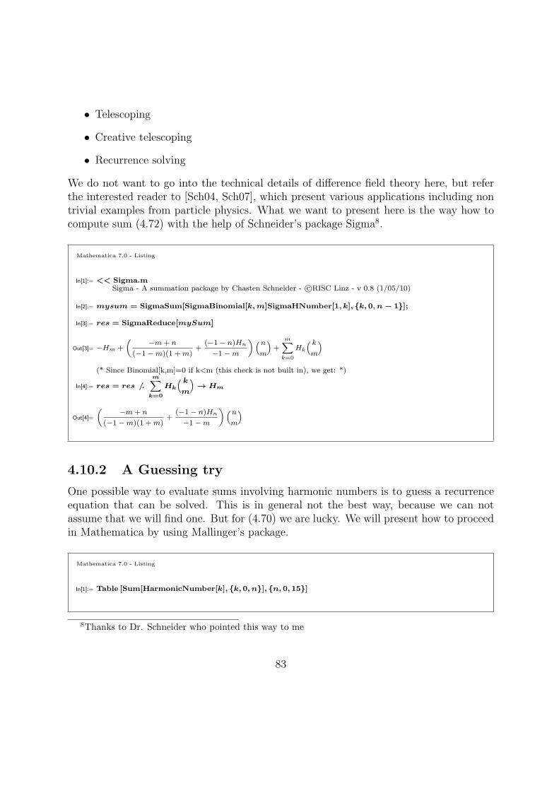
• Telescoping
• Creative telescoping
• Recurrence solving
We do not want to go into the technical details of difference field theory here, but referthe interested reader to [Sch04, Sch07], which present various applications including nontrivial examples from particle physics. What we want to present here is the way how tocompute sum (4.72) with the help of Schneider’s package Sigma8.
Mathematica 7.0 - Listing
In[1]:= << Sigma.mSigma - A summation package by Chasten Schneider - c⃝RISC Linz - v 0.8 (1/05/10)
In[2]:= mysum = SigmaSum[SigmaBinomial[k,m]SigmaHNumber[1, k], {k, 0, n − 1}];
In[3]:= res = SigmaReduce[mySum]
Out[3]= −Hm +
(−m+ n
(−1−m)(1 +m)+
(−1− n)Hn
−1−m
)(n
m
)+
m∑k=0
Hk
( k
m
)(* Since Binomial[k,m]=0 if k<m (this check is not built in), we get: *)
In[4]:= res = res /.m∑
k=0
Hk
( k
m
)→ Hm
Out[4]=
(−m+ n
(−1−m)(1 +m)+
(−1− n)Hn
−1−m
)(n
m
)
4.10.2 A Guessing try
One possible way to evaluate sums involving harmonic numbers is to guess a recurrenceequation that can be solved. This is in general not the best way, because we can notassume that we will find one. But for (4.70) we are lucky. We will present how to proceedin Mathematica by using Mallinger’s package.
Mathematica 7.0 - Listing
In[1]:= Table [Sum[HarmonicNumber[k], {k, 0, n}], {n, 0, 15}]
8Thanks to Dr. Schneider who pointed this way to me
83
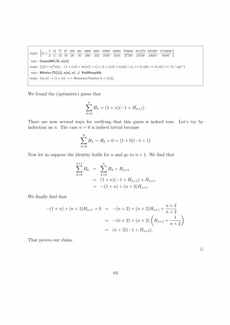
Out[1]=
{0, 1,
5
2,13
3,77
12,87
10,223
20,481
35,4609
280,4861
252,55991
2520,58301
2310,785633
27720,811373
25740,835397
24024,1715839
45045
}In[2]:= GuessRE [%, a[n]]
Out[2]= {{(2 + n)2a[n]− (1 + n)(5 + 2n)a[1 + n] + (1 + n)(2 + n)a[2 + n] == 0, a[0] == 0, a[1] == 1}, ”ogf”}
In[3]:= RSolve [%[[1]], a[n], n] // FullSimplify
Out[3]= {{a [n] → (1 + n)(−1 + HarmonicNumber [1 + n])}}
We found the (optimistic) guess that
n∑k=0
Hk = (1 + n)(−1 +Hn+1).
There are now several ways for verifying that this guess is indeed true. Let’s try byinduction on n. The case n = 0 is indeed trivial because
0∑k=0
Hk = H0 = 0 = (1 + 0)(−1 + 1)
Now let us suppose the identity holds for n and go to n+ 1. We find that
n+1∑k=0
Hk =n∑
k=0
Hk +Hn+1
= (1 + n)(−1 +Hn+1) +Hn+1
= −(1 + n) + (n+ 2)Hn+1.
We finally find that
−(1 + n) + (n+ 2)Hn+1 + 0 = −(n+ 2) + (n+ 2)Hn+1 +n+ 2
n+ 2
= −(n+ 2) + (n+ 2)
(Hn+1 +
1
n+ 2
)= (n+ 2)(−1 +Hn+2).
That proves our claim.
2
84
4.10.3 Applying the Egorychev method
Now we will use again the method of coefficients and generating functions to derive result(4.70). Before we need knowledge about the generating function of harmonic numbers.
Lemma 4.10.1 The generating function of the harmonic numbers is given by
∞∑n=0
Hnzn = − log(1− z)
1− z(4.73)
Proof. An equivalent definition of harmonic numbers is given by the recurrence
H0 = 0
Hn =1
n+Hn−1, n ≥ 1.
From the second line we find that
Hn+1 = Hn +1
n+ 1, n ≥ 0.
Now
H(z) =∞∑n=0
Hn+1zn+1 =
∞∑n=0
Hnzn+1 +
∞∑n=0
1
n+ 1zn+1
⇔ H(z) = zH(z)− log(1− z)
⇔ H(z) = − 1
1− zlog(1− z)
2
By Lemma 2.2.9, we know now that the harmonic numbers have the residue representation
Hk = resz
− log(1− z)
1− zz−k−1, k ≥ 0. (4.74)
If we now calculate sum (4.70) we find that
n∑k=0
Hk =n∑
k=0
resz
− log(1− z)
1− zz−k−1
= resz
− log(1− z)
1− z
1
z
n∑k=0
z−k
= resz
− log(1− z)
1− z
z−n−1 − 1
1− z
= resz
− log(1− z)
(1− z)2z−n−1 − res
z
log(1− z)
(1− z)2
85
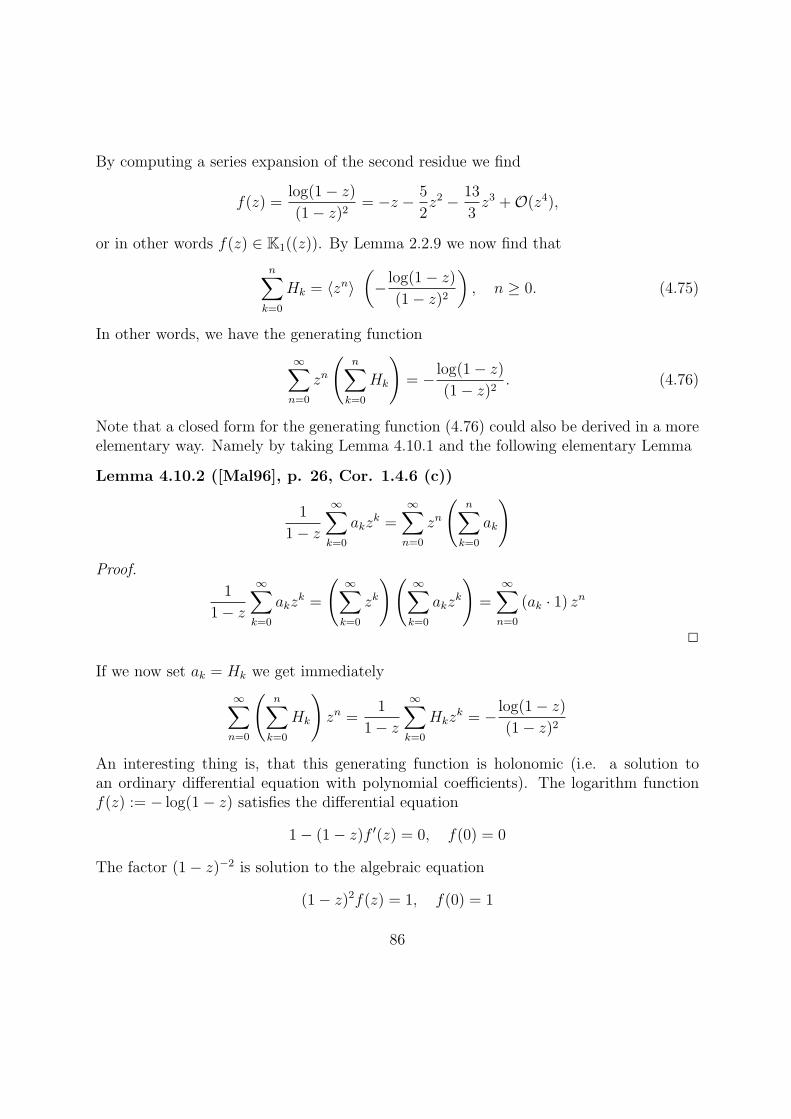
By computing a series expansion of the second residue we find
f(z) =log(1− z)
(1− z)2= −z − 5
2z2 − 13
3z3 +O(z4),
or in other words f(z) ∈ K1((z)). By Lemma 2.2.9 we now find that
n∑k=0
Hk = ⟨zn⟩(− log(1− z)
(1− z)2
), n ≥ 0. (4.75)
In other words, we have the generating function
∞∑n=0
zn
(n∑
k=0
Hk
)= − log(1− z)
(1− z)2. (4.76)
Note that a closed form for the generating function (4.76) could also be derived in a moreelementary way. Namely by taking Lemma 4.10.1 and the following elementary Lemma
Lemma 4.10.2 ([Mal96], p. 26, Cor. 1.4.6 (c))
1
1− z
∞∑k=0
akzk =
∞∑n=0
zn
(n∑
k=0
ak
)Proof.
1
1− z
∞∑k=0
akzk =
(∞∑k=0
zk
)(∞∑k=0
akzk
)=
∞∑n=0
(ak · 1) zn
2
If we now set ak = Hk we get immediately
∞∑n=0
(n∑
k=0
Hk
)zn =
1
1− z
∞∑k=0
Hkzk = − log(1− z)
(1− z)2
An interesting thing is, that this generating function is holonomic (i.e. a solution toan ordinary differential equation with polynomial coefficients). The logarithm functionf(z) := − log(1− z) satisfies the differential equation
1− (1− z)f ′(z) = 0, f(0) = 0
The factor (1− z)−2 is solution to the algebraic equation
(1− z)2f(z) = 1, f(0) = 1
86
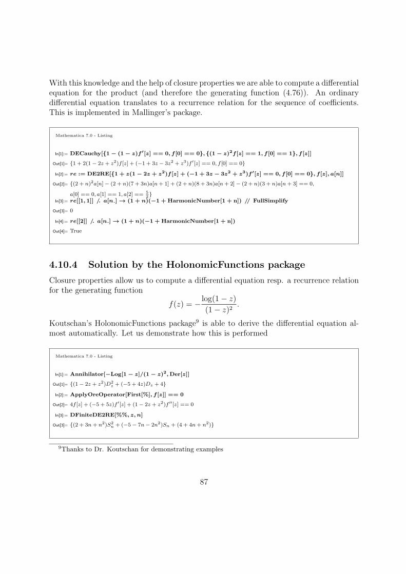
With this knowledge and the help of closure properties we are able to compute a differentialequation for the product (and therefore the generating function (4.76)). An ordinarydifferential equation translates to a recurrence relation for the sequence of coefficients.This is implemented in Mallinger’s package.
Mathematica 7.0 - Listing
In[1]:= DECauchy[{1 − (1 − z)f ′[z] == 0, f [0] == 0}, {(1 − z)2f [z] == 1, f [0] == 1}, f [z]]
Out[1]= {1 + 2(1− 2z + z2)f [z] + (−1 + 3z − 3z2 + z3)f ′[z] == 0, f [0] == 0}
In[2]:= re := DE2RE[{1 + z(1 − 2z + z2)f [z] + (−1 + 3z − 3z2 + z3)f ′[z] == 0, f [0] == 0}, f [z], a[n]]
Out[2]= {(2 + n)2a[n]− (2 + n)(7 + 3n)a[n+ 1] + (2 + n)(8 + 3n)a[n+ 2]− (2 + n)(3 + n)a[n+ 3] == 0,
a[0] == 0, a[1] == 1, a[2] == 52}
In[3]:= re[[1, 1]] /. a[n ] → (1 + n)(−1 + HarmonicNumber[1 + n]) // FullSimplify
Out[3]= 0
In[4]:= re[[2]] /. a[n ] → (1 + n)(−1 + HarmonicNumber[1 + n])
Out[4]= True
4.10.4 Solution by the HolonomicFunctions package
Closure properties allow us to compute a differential equation resp. a recurrence relationfor the generating function
f(z) = − log(1− z)
(1− z)2.
Koutschan’s HolonomicFunctions package9 is able to derive the differential equation al-most automatically. Let us demonstrate how this is performed
Mathematica 7.0 - Listing
In[1]:= Annihilator[−Log[1 − z]/(1 − z)2,Der[z]]
Out[1]= {(1− 2z + z2)D2z + (−5 + 4z)Dz + 4}
In[2]:= ApplyOreOperator[First[%], f [z]] == 0
Out[2]= 4f [z] + (−5 + 5z)f ′[z] + (1− 2z + z2)f ′′[z] == 0
In[3]:= DFiniteDE2RE[%%, z, n]
Out[3]= {(2 + 3n+ n2)S2n + (−5− 7n− 2n2)Sn + (4 + 4n+ n2)}
9Thanks to Dr. Koutschan for demonstrating examples
87
Hence, f(z) satisfies the differential equation
(1− 2z + z2)f ′′(z) + (−5 + 5z)f ′(z) + 4f(z) = 0
and on coefficient level
(2 + 3n+ n2)f(n+ 2) + (−5− 7n− 2n2)f(n+ 1) + (4 + 4n+ n2)f(n) = 0
But how are this differential equations related? In fact they are equivalent, except that thesecond is a homogenous differential equation. In particular, if we differentiate Mallinger’sdifferential equation
d
dz
(1 + 2(1− 2z + z2)f [z] + (−1 + 3z − 3z2 + z3)f ′[z] = 0
)→ (−1 + z)(4f [z] + (−1 + z)(5f ′[z] + (−1 + z)f ′′[z])) = 0
which is (up to multiplication by (−1+z)) exactly Koutschan’s differential equation. Thereason for this is that if f(z) ∈ K[[z]] the linear space spanned by
⟨{f (k)(z) | k ∈ N
}⟩K(z)
=
⟨{dk
dzkf(z) | k ∈ N
}⟩K(z)
is a finite dimensional subspace of K((z)) over K(z). Hence there are many ways ofdescribing the same object. As an example consider (for k ∈ N) the differential equation
dk
dzkf(z)− f(z) = 0,
and the initial condition(
dm
dzmf(z)
)|z=0 = C0 where 0 ≤ m ≤ k − 1, C0 ∈ K. This system
of differential equations has the unique solution
f(z) = C0ez,
although there are infinitely many equations describing f(z). With an appropriate choiceof initial values we can ensure uniqueness of the result.
4.10.5 Application of change of variables
In the text examples of [Ego84], Egorychev demonstrates his method by proving theidentity
S(n) :=n∑
k=1
(−1)k−1
(n
k
)Hk =
1
n.
88
In fact he proceeded the same lines as we did and arrives at the residue representation
n∑k=1
(−1)k−1
(n
k
)Hk = res
u
(1 + u)n−1 log(1− u)
un+1.
But now a miracle happens. If one substitutes
w =u
1 + u∈ K1((u)) ↔ u =
w
1− w,
according to rule 5 we get
resu
(1 + u)n−1 log(1− u)
un+1= − res
w
log(1− w)
wn+1,
or in other words the coefficient of wn in the series expansion of − log(1−w). But this isknown explicitly in closed form. Namely we find that
S(n) = − resw
log(1− w)
wn+1=
1
n.
4.11 Analytic aspects
One reason, why formal power series are that powerful is that we can look at them fromdifferent points of view. So far we have manipulated them in a purely formal way. Let usnow suppose, we have given a generating function in closed form and we want to extractinformation about the asymptotic growth of the coefficient sequence. That is, we want togive an estimate about the size of the n’th element of the sequence (fn)n≥0 that has thegenerating function f(z). In general [FS09, p. 226] this will look like
⟨zn⟩ f(z) = ⟨zn⟩∞∑n=0
fnzn = fn = Anθ(n), (4.77)
where we call An the exponential growth part and θ(n) the subexponential part. In [FS09,p. 227] the two main principles for extracting asymptotic information about the sequenceare described as follows
• First Principle of Coefficient Asymptotics The location of a function’s singu-larities dictates the exponential growth (An) of its coefficients
89
• Second Principle of Coefficients Asymptotics The nature of a function’s sin-gularities determines the associate subexponential factor (θ(n))
The exponential factor A is related to the radius of convergence of a series. As it turnsout, the rate of growth is given by
A =1
ρ=
1
lim supn→∞
n√
|fn|, (4.78)
where ρ is the first singularity encountered along the positive real axis ([FS09, p. 226]).With the help of complex analysis one is able to determine formulas for the asymptoticgrowth of the coefficients in the power series expansion. We consider the case where we donot find an explicit closed form as it might be the case in examples involving logarithmicfactors.
Theorem 4.11.1 ([FS09], p.385, Thm. VI.2) Let α be an arbitrary complex numberin C \ Z≤0. The coefficient of zn in the function
f(z) = (1− z)−α
(1
zlog
(1
1− z
))β
admits for a large n a full asymptotic expansion in descending powers of log(n),
fn = ⟨zn⟩ f(z) ∼ nα−1
Γ(α)(log(n))β
[1 +
C1
log(n)+
C2
log(n)2+ . . .
]where
Ck =
(β
k
)Γ(α)
dk
dsk1
Γ(s)|s=α
Proof. The proof uses complex integration methods and is a consequence of the precedingtheorem VI.1 in [FS09]. For the full details see [FS09, p. 385]. 2
Remark: Γ(α) denotes the Eulerian Gamma function defined by
Γ(α) :=
∫ ∞
0
e−ttα−1 dt (4.79)
In the book there are several special cases pointed out explicitly namely the cases whereα = 1
2and β = −1. Also the case where α is a nonnegative integer is interesting,
because in this case the Gamma function evaluates to a simple factorial by the wellknown interpolation property
∀n ∈ N : Γ(n+ 1) = n!
that is easily proved by integration by parts.
90
Curriculum Vitae
Christoph Furst
Brunngasse 2A-4310 Mauthausen
E-Mail: [email protected]
Date and Place of Birth: November 13, 1986, LinzNationality: Austria
Education:
1993-2001 Classical Education, Mauthausen
2001-2006 Technical High School HTBLA Steyr, Austria,
Educational Focus on Electronics and Technical Informatics
2006-2009 Bachelor Studies in Technical Mathematics, Johannes Kepler University Linz
Completed with distinction on 28.09.2009, Academic Degree: Bachelor of Science
2009-now Master Studies in Technical Mathematics, Johannes Kepler University Linz
Educational Focus on Computer Mathematics
91
Bibliography
[AAR99] George E. Andrews, Richard Askey, and Ranjan Roy. Special Functions.Number 71 in Encyclopedia Math. Appl. Cambridge Univ. Press, Cambridge,1999.
[APR01] G.E. Andrews, P. Paule, and A. Riese. MacMahon’s Partition Analysis IX:k-gon partitions. Bull. Austral. Math. Soc., 64:321–329, 2001.
[Ego84] Gregory P. Egorychev. Integral Representation and the Computation ofCombinatorial Sums. Trans. from the Russian (Translations of Mathemat-ical Monographs) Vol. 59. American Mathematical Society, December 1984.
[FB07] Eberhard Freitag and Rolf Busam. Funktionentheorie 1. Springer, 2007.
[FS09] Philippe Flajolet and Robert Sedgewick. Analytic Combinatorics. CambridgeUniversity Press, 2009.
[GCL92] Keith O. Geddes, Stephen R. Czapor, and George Labahn. Algorithms forComputer Algebra. Kluwer Academic Publishers, Norwell, MA, USA, 1992.
[GKP94] Ronald L. Graham, Donald E. Knuth, and Oren Patashnik. Concrete Math-ematics: A Foundation for Computer Science. Addison-Wesley LongmanPublishing Co., Inc., Boston, MA, USA, 1994.
[Gos78] R W Gosper. Decision procedure for indefinite hypergeometric summation.Proc Natl Acad Sci U S A, 75(1):40–2, 1978.
[HS09] Tian-Xiao He and Renzo Sprugnoli. Sequence characterization of riordanarrays. Discrete Mathematics, 309(12):3962 – 3974, 2009.
[Kau07] Manuel Kauers. Summation algorithms for Stirling number identities. Jour-nal of Symbolic Computation, 42(10):948–970, October 2007.
[Kou09] Christoph Koutschan. Advanced Applications of the Holonomic Systems Ap-proach. PhD thesis, RISC-Linz, Johannes Kepler University, September 2009.
92
[Kou10] Christoph Koutschan. HolonomicFunctions (User’s Guide). Technical Report10-01, RISC Report Series, University of Linz, Austria, January 2010.
[KP11] Manuel Kauers and Peter Paule. The Concrete Tetrahedron. Text and Mono-graphs in Symbolic Computation. Springer Wien, 1st edition, 2011.
[Mal96] C. Mallinger. Algorithmic Manipulations and Transformations of Univari-ate Holonomic Functions and Sequences. Master’s thesis, RISC, J. KeplerUniversity, August 1996.
[MRSV97] Donatella Merlini, Douglas Rogers, Renzo Sprugnoli, and Cecilia Verri. Onsome alternative characterizations of Riordan arrays. Canadian J. Mathe-matics, 49:301–320, 1997.
[Pet98] Marko Petkovsek. Hypergeometric solutions of linear recurrences with poly-nomial coefficients. Journal of Symbolic Computation, 11:1–22, 1998.
[PS95] Peter Paule and Markus Schorn. A Mathematica version of Zeilberger’s algo-rithm for proving binomial coefficient identities. Journal of Symbolic Com-putation, 20(5-6):673–698, 1995.
[PWZ96] M. Petkovsek, H. S. Wilf, and D. Zeilberger. A = B. A. K. Peters, Wellesley,1996.
[Rio68] J. Riordan. Combinatorial Identities. John Wiley, New York, 1968.
[Ros97] M. Rosenkranz. Lagrange Inversion. Master’s thesis, RISC, J. Kepler Uni-versity Linz, 1997.
[Sch01] C. Schneider. Symbolic Summation in Difference Fields. PhD thesis, RISC, J.Kepler University Linz, May 2001. (Published as Technical report no. 01-17in RISC Report Series.).
[Sch04] C. Schneider. The summation package Sigma: Underlying principles and arhombus tiling application. Discrete Math. Theor. Comput. Sci., 6(2):365–386, 2004.
[Sch07] C. Schneider. Symbolic summation assists combinatorics. Sem. Lothar. Com-bin., 56:1–36, 2007. Article B56b.
[SGWW91] Louis W. Shapiro, Seyoum Getu, Wen-Jin Woan, and Leon C. Woodson. TheRiordan group. Discrete Applied Mathematics 34, 229-239, 1991.
93
[Spr94] Renzo Sprugnoli. Riordan arrays and combinatorial sums. Discrete Math.,132(1-3):267–290, 1994.
[Spr95] Renzo Sprugnoli. Riordan arrays and the Abel-Gould identity. DiscreteMath., 142(1-3):213–233, 1995.
[Spr06] Renzo Sprugnoli. An Introduction to Mathematical Methods in Combina-torics, available at http: // www. dsi. unifi. it/ ~ resp/ Handbook. pdf .[Abgerufen: 14. Oktober 2010], 2006.
[Spr07] Renzo Sprugnoli. Riordan array proofs of identities in Goulds book, availableat http: // www. dsi. unifi. it/ ~ resp/ GouldBK. pdf . [Abgerufen: 14.Oktober 2010], 2007.
[Sta86] R P Stanley. Enumerative Combinatorics, volume 1. Wadsworth Publ. Co.,Belmont, CA, USA, 1986.
[Wil06] Herbert S. Wilf. Generatingfunctionology. A. K. Peters, Ltd., Natick, MA,USA, 2006.
94


![A Combinatorial Proof of a Theorem of Katsuuraramanujan.math.trinity.edu/bmiceli/research/KatsuuraCJM.pdfDence [2], in working with Laplace transforms and row-sums on Pascal’s triangle,](https://img.dokumen.tips/doc/110x75/60a50bef8690e966367008fe/a-combinatorial-proof-of-a-theorem-of-dence-2-in-working-with-laplace-transforms.jpg)