Embed Size (px)
Citation preview

1
Combinatorial Optimization
Winter course 2018/2019
Prof. Dr. Stefan Bock
University of Wuppertal
Business Computing and Operations Research
Business Computing and Operations Research 2
Information concerning the course
� Lecture: � Monday, 2:15 pm - 3:45 pm in M12.25
� Thursday, 2:15 pm - 3:45 pm in M12.25
� Start: October 11th, 2018
� Lecturer: Prof. Dr. Stefan Bock� Office: M12.02
� Office hour: Monday, 4:00 pm - 6:00 pm (registration is mandatory (email to [email protected]))
� Secretary office: M12.01
� E-mail: [email protected]
Business Computing and Operations Research 3
Information concerning the course
� Tutorial: � Wednesday, 2:00 pm - 4:00 pm in M.15.09
� Start: October 17th, 2018
� First assignment sheet is already available
� Supervisor: Anna Katharina Janiszczak� Office: M12.33
� Office hour: Wednesday, 4:00 pm-6:00 pm (after agreement (per email))
� E-mail: [email protected]
� Coordinates the Tutorial
Business Computing and Operations Research 4
Information concerning the course
� Weekly assignment sheet submission� Submit in Moodle as PDF or postbox in room M11.25� Write down course name and make sure you can
identify your submission on return
Mo Thu
Lecture
Assignments online in Moodle
10 am: due date for assignment sheet submission
2 pm: Tutorial: Assignment review
Wed

2
Business Computing and Operations Research 5
Preliminary Agenda
1. Linear programming 1. Applications
2. The Simplex Algorithm
3. Geometry of the solution space
4. How fast is the Simplex Method?
5. Working with tableaus
2. Duality1. Motivation and the dual problem
2. The Dual Simplex Algorithm
3. The possible cases
4. Interpreting the dual solution
5. Farkas’ Lemma
Business Computing and Operations Research 6
Preliminary Agenda
3. Computational considerations1. The Revised Simplex Algorithm
2. Analyzing the complexity of the Revised Simplex Algorithm
3. Solving the Max Flow Problem by the Revised Simplex Algorithm
4. The Dantzig-Wolfe Decomposition
4. The Hitchcock Transportation Problem1. Using the standardized Simplex Algorithm
2. The MODI Algorithm
5. The Primal-Dual Simplex Algorithm
Business Computing and Operations Research 7
Preliminary Agenda
6. Optimally solving the Shortest Path Problem1. Deriving the Dijkstra algorithm
2. Bellman-Ford algorithm
3. The Floyd-Warshall algorithm
7. Max-Flow and Min Cut Problems1. Max-Flow Problems
2. Min-Cut Problems
3. A Primal-Dual algorithm
4. The Ford-Fulkerson algorithm
5. Analyzing the Ford-Fulkerson algorithm
6. An efficient algorithm for the Max-Flow Problem
Business Computing and Operations Research 8
Preliminary Agenda
8. Applying the Primal-Dual Simplex to the Transportation Problem – The alpha-beta algorithm
1. Problem definition and analysis
2. Analyzing the reduced primal (RP)
3. Solving the DRP
4. Complexity of the algorithm
9. Integer programming1. Basics
2. Cutting Plane Methods – algorithm of Gomory
3. A Branch&Bound Algorithm

3
Business Computing and Operations Research 9
Preliminary Agenda
10. Matrix Games1. Introducing examples
2. Basic definitions
3. Games and Linear Programming
Business Computing and Operations Research 10
Selected basic Literature
� Brucker, P.; Knust, S. (2012): Complex Scheduling. 2. ed., Springer, Berlin, Heidelberg, New York.
� Domschke, W.; Drexl, A.; Klein, R.; Scholl, A.; Voß, S. (2015): Übungen und Fallbeispiele zum OperationsResearch. 8. Aufl., Springer Gabler, 2015.
� Domschke, W.; Drexl, A. (2015): Einführung in OperationsResearch. 9. Aufl., Springer Gabler.
� Myerson, R.B. (1997): Game Theory. Analysis of Conflict. Havard University Press.
� Nemhauser,G.L.,&Wolsey,L.A.(1988).Integer andcombinatorial optimization. JohnWiley&Sons, New York.
� Papadimitriou, C.H.; Steiglitz, K. (1982, 1988): Combinatorial Optimization. Algorithms and Complexity. Prentice-Hall, 1982 and Dover unabridged edition 1998.
Business Computing and Operations Research 11
Selected basic Literature
� Suhl, L.; Mellouli, T. (2013): Optimierungssysteme. 3. Aufl., Springer Gabler.
� Taha, H.A. (2010): Operations Research. An Introduction. 9th ed, Pearson Education.
� Chvátal, V. (2002): Linear Programming. 16th print. W.H. Freeman and Company, New York.
� Wolsey, L.A. (1998): Integer Programming. John Wiley&Sons.
And thousands of other good books dealing with Optimization, Linear Programming, or Combinatorial Optimization (references to further papers will be given in the respective sections)
Business Computing and Operations Research 12
Simplex calculators
� Excel Solver� Can be activated under Extras⇢Add-Ins (2003
Version), File⇢Options⇢Add-Ins (2010 Version)
� Subsequently, you may use the Solver by Extras⇢Solver (2003 Version), Data⇢Solver (2010 Version)
� It is not powerful but nice to play around with our simple examples
� Online Simplex calculator:
http://www.zweigmedia.com/RealWorld/simplex.html

4
Business Computing and Operations Research 13
1 Linear Programming
� We deal with a large class of problems in this first section
� These problems can be mapped as Linear Programs, i.e., � We define continuous variables
� We define linear constraints to be fulfilled by the values of the variables
� We define an objective function that provides an evaluation of each solution found
� We want to find optimal solutions, i.e., solutions that fulfill all restrictions (then we denote them as feasible) and maximize or minimize the objective function value
Business Computing and Operations Research 14
Linear Program – Main attributes
� continuous decision variables
� linear constraints that must be fulfilled by the values of the decision variables
� objective function that provides an evaluation of each solution found
� Finding an optimal solution
Solution: vector of decision variables
Feasible solution: solution that fulfills all constraints
Optimal solution: feasible solution with maximal or minimal objective function value
Business Computing and Operations Research 15
1.1 Linear Programming Applications
� We commence our work with representative applications of Linear Programming
� Production Program Planning
� Hitchcock problem, i.e., standardized balanced transportation problem
� Diet Problem
Business Computing and Operations Research 16
Application 1 – Production Program Planning
� The production management of a plant of an orange juice producer plans the production program
� There are two types of orange juices that are pressed and mixed in this plant
� For simplicity reasons, let us denote them as A and B
� Both are produced on 3 stages in a predetermined sequence, i.e., 1 – 2 – 3 is the production sequence for both product types
� This is illustrated by the following figure

5
Business Computing and Operations Research 17
Production Program Planning - Illustration
Stage 1
Stage 2
Stage 3
A
B
10 $
Max. amount50
8 $
Max. amount40
Capacity240 h
Capacity240 h
Capacity100 h
Business Computing and Operations Research 18
' and just the values
� All types are produced on all stages
� Capacity on stages 1 and 3 are 240 h,
� Capacity on stage 2 is 100 h
� Product A
� Price per gallon: 10$
� Variable costs per gallon: 5$
� Thus, we obtain a marginal profit of 5$ per gallon
� Max. sales volume: 50 gallons
� In order to produce one gallon of A � on stage 1, we need 2 hours,
� on stage 2, 1 hour,
� and on stage 3, 4 hours
Business Computing and Operations Research 19
' and product B
� Product B� Price per gallon: 8$
� Variable costs per gallon: 2$
� Thus, we obtain a marginal profit of 6$ per gallon
� Max. sales volume: 40 gallons
� In order to produce one gallon of B � on stage 1, A gallon B requires 4 hours
� on stage 2, A gallon B requires 2 hours, and
� on stage 3, A gallon B requires 2 hours
Business Computing and Operations Research 20
Optimal production program
� Clearly, we want to maximize our profit, i.e., the maximally obtainable total marginal profit
� Thus, we analyze what we are able to sell maximally� Both types of orange juice are worth to produce� Each item of A brings us a marginal profit of 5$ per
gallon� Each item of B even 6$
� Consequently, we want to produce as much as possible of both products
� If the maximum volumes of sale can be produced, we have found the optimal production program

6
Business Computing and Operations Research 21
We calculate the maximum demand
� We have the following demand levels
� Stage 1: 50.2+40.4=260>240
Thus, since demand is larger than capacity, we have a bottleneck !
� Stage 2: 50.1+40.2=130>100
Thus, since demand is larger than capacity, we have a bottleneck !
� Stage 3: 50.4+40.2=280>240
Thus, since demand is larger than capacity, we have a bottleneck !
Business Computing and Operations Research 22
What is to do?
?
Since B provides 6$ instead of 5$,
we produce as much as possible of B; and then we
fill up the rest with A
Since B provides 6$ instead of 5$,
we produce as much as possible of B; and then we
fill up the rest with A
Business Computing and Operations Research 23
If we do so, it turns out that '
� B needs
� on stage 1 4h. Maximally produce min{40, 240/4} = 40
� on stage 2 2h. Maximally produce min{40, 100/2} = 40
� on stage 3 2h. Maximally produce min{40, 240/2} = 40
Thus, B can be produced in its maximum volume of sales
� A needs
� on stage 1 2h. Maximally produce min{50, (240-160)/2} = 40
� on stage 2 1h. Maximally produce min{50, (100-80)/1=20/1} = 20
� on stage 3 4h. Maximally produce min{50, (240-80)/4=160/4} = 40
Thus, 20 items of A can be additionally produced and sold
Business Computing and Operations Research 24
Results in
a total profit of
20.5$ + 40.6$ = 100$ + 240$ = 340$
� However, in order to analyze the problem more in detail, we want to formalize it

7
Business Computing and Operations Research 25
Linear Program of the production
Decision variables: : Produced gallons of juice A
: Produced gallons of juice B
Objective function: Maximize 5 6 Maximize the total revenue
Constraints: subject to
50 Maximium volume of sales
40
A
B
A B
A
B
x
x
z x x
x
x
= ⋅ + ⋅
≤
≤
2 4 240 Production capacities
1 2 100
4 2 240
, 0 Non-negativity constraints
A B
A B
A B
A B
x x
x x
x x
x x
⋅ + ⋅ ≤
⋅ + ⋅ ≤
⋅ + ⋅ ≤
≥
Business Computing and Operations Research 26
Graphical solutionxA
10050 7525
25
50
75
100Restriction 1
xB
Restriction 3Z=500Restriction 2
Optimal solution
Business Computing and Operations Research 27
Optimal solution
� Obviously, the optimal solution is located at the point of intersection of restriction 2 and 3
� Thus, we have to solve
( )
6,26
6,46
3/80
3/140
3/80
3/1603/300
3/80
2100
1203200
2100
1204200
2100
12021002
2100
1202
2100
24024
10021
=
=⇔
=
=⇔
=
−=⇔
=
⋅−=⇔
=⋅−
⋅−=⇔
=+⋅−
⋅−=⇔
=+⋅−⋅
⋅−=⇔
=+⋅
⋅−=⇔
=⋅+⋅
=⋅+⋅
B
A
B
A
B
A
B
BA
B
BA
BB
BA
BB
BA
BA
BA
BA
BA
x
x
x
x
x
x
x
xx
x
xx
xx
xx
xx
xx
xx
xx
xx
xx
Business Computing and Operations Research 28
Results in
a total (optimal) profit of
26.6.6$ + 46.6.5$ = 233.3$ + 159.9$ = 393.3$

8
Business Computing and Operations Research 29
Consequence
OK !I admit that I was wrong!
However, what can we do if there are more than 2
variables??
OK !I admit that I was wrong!
However, what can we do if there are more than 2
variables??
Then, we will formulate a general version of that LP
and use the SIMPLEX
ALGORITHM
Then, we will formulate a general version of that LP
and use the SIMPLEX
ALGORITHM
Business Computing and Operations Research 30
Production Program Planning
[ ]
[ ][ ]
,
: Marginal profit per item of product type 1,..., MU/PU
: Production coefficient of product type 1,..., on machine
1,..., CU/PU
: Maximum capacity of machine 1,..., CU
: Maximum number
j
i j
i
j
p j n
c j n
i m
C i m
X
=
=
=
=
[ ]
[ ]
{ }
1
,
of items of product type 1,..., salable in
the planning horizon PU
: Number of items of product type 1,..., to be produced
in the planning horizon PU
Maximize
subject to 1,..., :
j
n
j j
j
i j
j n
x j n
p x
i m c
=
=
=
⋅
∀ ∈
∑
{ }1
1,..., : 0
n
j i
j
j j
x C
j n x X
=
⋅ ≤
∀ ∈ ≤ ≤
∑
Business Computing and Operations Research 31
Using Excel
� The program Excel comprises a standard solver for Linear Programs
� It is neither really high-performance nor convenient to use but available and sufficient for our exemplary problem constellations
� Activate the Solver by Extras⇢Add-Ins (2003 Version), File⇢Options⇢Add-Ins (2010 Version)
� Subsequently, you may use the Solver by Extras⇢Solver(2003 Version), Data⇢Solver (2010 Version)
� Let us try it outV
Microsoft
Excel-Arbeitsblatt
Business Computing and Operations Research 32
Application 2 – The Hitchcock Problem
� A service agent has three sales offices (CX, CY, and CZ) in Wuppertal
� These offices are supplied by three local printing plants (PA, PB, and PC)
� In order to satisfy the numerous soccer fans in Wuppertal, the service agent has an exclusive license of sale for the famous football/soccer club Borussia Mönchengladbach
� While the tickets are printed in the printing plants at equal costs, the transport to the offices causes individual costs
� Additional information� Each printing plant has an individual inventory for the next day.
Note that this inventory is extremely perishable
� Each sales office has an individual maximum amount of sales

9
Business Computing and Operations Research 33
The Hitchcock Problem – Illustration
Printing Plant A
4 pallets
Printing Plant B7 pallets
Printing Plant C2 pallets
Sales Office X
Demand: 2 pallets
Sales Office Z
Demand: 6 pallets
Sales Office Y
Demand: 5 pallets
Business Computing and Operations Research 34
The Matrix
Producers
A B C
Supply 4 7 2
Consumers
X Y Z
Demand 2 5 6
Business Computing and Operations Research 35
Transportation Distances
Distance X Y Z
A 2 3 4
B 4 6 8
C 5 2 7
Business Computing and Operations Research 36
What is the objective?
� Obviously, we have to decide about the quantities to be transported along each relation between a printing plant and a ticket office
� Specifically, we determine the precise number of product units that are transported along each relation
� Since quality is assumed to be negligible, a transportation cost minimization is appropriate to compare generated assignments
� Thus, a solution is solely rated by the incurred transportation costs

10
Business Computing and Operations Research 37
Let’s solve the problem
� When you try something out, you usually provide a heuristic solution
� Heuristic solutions do not always guarantee a certain quality
� Usually, their performance is empirically validated or roughly anticipated for worst case scenarios
� In the following, we want to obtain some insights into the problem structure by applying some well-known simple heuristics
Business Computing and Operations Research 38
Minimum Method
� Basic idea:
“Find the least possible combination of costs and
use it exhaustively. Afterwards, proceed with the
second lowest one,�”
� Let us do soV
Business Computing and Operations Research 39
Minimum Method
Distance X D:2 Y D:5 Z D:6
A S:4 (2) 0 (3) 0 (4) 0
B S:7 (4) 0 (6) 0 (8) 0
C S:2 (5) 0 (2) 0 (7) 0
Business Computing and Operations Research 40
Minimum Method
Distance X D:0 Y D:5 Z D:6
A S:2 (2) 2 (3) 0 (4) 0
B S:7 (4) 0 (6) 0 (8) 0
C S:2 (5) 0 (2) 0 (7) 0

11
Business Computing and Operations Research 41
Minimum Method
Distance X D:0 Y D:3 Z D:6
A S:2 (2) 2 (3) 0 (4) 0
B S:7 (4) 0 (6) 0 (8) 0
C S:0 (5) 0 (2) 2 (7) 0
Business Computing and Operations Research 42
Minimum Method
Distance X D:0 Y D:1 Z D:6
A S:0 (2) 2 (3) 2 (4) 0
B S:7 (4) 0 (6) 0 (8) 0
C S:0 (5) 0 (2) 2 (7) 0
Business Computing and Operations Research 43
Minimum Method
Distance X D:0 Y D:1 Z D:6
A S:0 (2) 2 (3) 2 (4) 0
B S:7 (4) 0 (6) 0 (8) 0
C S:0 (5) 0 (2) 2 (7) 0
Business Computing and Operations Research 44
Minimum Method
Distance X D:0 Y D:1 Z D:6
A S:0 (2) 2 (3) 2 (4) 0
B S:7 (4) 0 (6) 0 (8) 0
C S:0 (5) 0 (2) 2 (7) 0

12
Business Computing and Operations Research 45
Minimum Method
Distance X D:0 Y D:1 Z D:6
A S:0 (2) 2 (3) 2 (4) 0
B S:7 (4) 0 (6) 0 (8) 0
C S:0 (5) 0 (2) 2 (7) 0
Business Computing and Operations Research 46
Minimum Method
Distance X D:0 Y D:0 Z D:6
A S:0 (2) 2 (3) 2 (4) 0
B S:6 (4) 0 (6) 1 (8) 0
C S:0 (5) 0 (2) 2 (7) 0
Business Computing and Operations Research 47
Minimum Method
Distance X D:0 Y D:0 Z D:6
A S:0 (2) 2 (3) 2 (4) 0
B S:6 (4) 0 (6) 1 (8) 0
C S:0 (5) 0 (2) 2 (7) 0
Business Computing and Operations Research 48
Minimum Method
Distance X D:0 Y D:0 Z D:0
A S:0 (2) 2 (3) 2 (4) 0
B S:0 (4) 0 (6) 1 (8) 6
C S:0 (5) 0 (2) 2 (7) 0
Total costs = 68

13
Business Computing and Operations Research 49
Vogel’s Approximation Method
� Basic Idea:
“Avoid larger deteriorations by identifying critical
relations”
� Specifically, calculate the differences between the best and the second best relation for all producers and all consumers
� Select the best relation for the one with the largest difference
� Proceed until a complete solution is found
Business Computing and Operations Research 50
Vogel’s Approximation Method
DistanceX D:2Diff: 2
Y D:5Diff: 1
Z D:6
Diff: 3
A S:4Diff: 1
(2) 0 (3) 0 (4) 0
B S:7Diff: 2
(4) 0 (6) 0 (8) 0
C S:2Diff: 3
(5) 0 (2) 0 (7) 0
Business Computing and Operations Research 51
Vogel’s Approximation Method
DistanceX D:2Diff: 1
Y D:5
Diff: 4Z D:2Diff: 1
A S:0Diff: 0
(2) 0 (3) 0 (4) 4
B S:7Diff: 2
(4) 0 (6) 0 (8) 0
C S:2Diff: 3
(5) 0 (2) 0 (7) 0
Business Computing and Operations Research 52
Vogel’s Approximation Method
DistanceX D:2Diff: 0
Y D:3Diff: 0
Z D:2Diff: 0
A S:0Diff: 0
(2) 0 (3) 0 (4) 4
B S:7
Diff: 2(4) 0 (6) 0 (8) 0
C S:0Diff: 0
(5) 0 (2) 2 (7) 0

14
Business Computing and Operations Research 53
Vogel’s Approximation Method
DistanceX D:0Diff: 0
Y D:3Diff: 0
Z D:2Diff: 0
A S:0Diff: 0
(2) 0 (3) 0 (4) 4
B S:5
Diff: 2(4) 2 (6) 0 (8) 0
C S:0Diff: 0
(5) 0 (2) 2 (7) 0
Business Computing and Operations Research 54
Vogel’s Approximation Method
DistanceX D:0Diff: 0
Y D:0Diff: 0
Z D:2Diff: 0
A S:0Diff: 0
(2) 0 (3) 0 (4) 4
B S:2
Diff: 2(4) 2 (6) 3 (8) 0
C S:0Diff: 0
(5) 0 (2) 2 (7) 0
Business Computing and Operations Research 55
Vogel’s Approximation Method
DistanceX D:0Diff: 0
Y D:0Diff: 0
Z D:0Diff: 0
A S:0Diff: 0
(2) 0 (3) 0 (4) 4
B S:0
Diff: 2(4) 2 (6) 3 (8) 2
C S:0Diff: 0
(5) 0 (2) 2 (7) 0
Total costs = 62
Business Computing and Operations Research 56
Local Improvement Operations
� We may improve an existing solution by applying specific transformation moves, i.e., we slightly modify a current solution in a way that� feasibility is maintained, and � solution quality is improved
� A simple example is the pairwise shift
� Specifically, we select two consumer-producer relations (P1&C1, P2&C2) and ask for the change in costs byV� transporting one unit from P1 to C2 rather than from P1
to C1
� For P2, we simultaneously consider the same� Note that feasibility is ensured by the simultaneous
consideration of both constellations

15
Business Computing and Operations Research 57
Pairwise shift
Distance X D:0 Y D:0 Z D:0
A S:0 (2) 2 (3) 2 (4) 0
B S:0 (4) 0 (6) 1 (8) 6
C S:0 (5) 0 (2) 2 (7) 0
Total Costs = 68
Business Computing and Operations Research 58
Pairwise shift
Distance X D:0 Y D:0 Z D:0
A S:0 (2) 0 (3) 2 (4) 2
B S:0 (4) 2 (6) 1 (8) 4
C S:0 (5) 0 (2) 2 (7) 0
Total Costs are 68-4=64
Business Computing and Operations Research 59
Pairwise shift
Distance X D:0 Y D:0 Z D:0
A S:0 (2) 0 (3) 2 (4) 2
B S:0 (4) 2 (6) 1 (8) 4
C S:0 (5) 0 (2) 2 (7) 0
Total Costs = 64
Business Computing and Operations Research 60
Pairwise shift
Distance X D:0 Y D:0 Z D:0
A S:0 (2) 0 (3) 0 (4) 4
B S:0 (4) 2 (6) 3 (8) 2
C S:0 (5) 0 (2) 2 (7) 0
Total Costs are 64-2=62

16
Business Computing and Operations Research 61
The (balanced) Transportation Problem
[ ][ ][ ]
,
,
: Delivery costs for each product unit that is transported from
supplier 1,..., to customer 1,..., CU/PU
: Total supply of 1,..., PU
: Total demand of 1,..., PU
: Quantity that su
i j
i
j
i j
c
i m j n
a i m
b j n
x
= =
=
=
[ ]
{ }
{ }
{ } { }
, ,
1 1
,
1
,
1
,
pplier 1,..., delivers to the customer 1,..., PU
Minimize
subject to 1,..., :
1,..., :
1,..., : 1,..., : 0
m n
i j i j
i j
n
i j i
j
m
i j j
i
i j
i m j n
c x
i m x a
j n x b
i m j n x
= =
=
=
= =
⋅
∀ ∈ =
∀ ∈ =
∀ ∈ ∀ ∈ ≥
∑∑
∑
∑
Business Computing and Operations Research 62
The balanced Transportation Problem
Printing Plant A
a[A]: 4 pallets
Printing Plant B
a[B]: 7 pallets
Printing Plant C
a[C]: 2 pallets
Sales Office X
b[x]: 2 pallets
Sales Office Z
b[z]: 6 pallets
Sales Office Y
b[y]: 5 pallets
( )
( ) ( )
,
2 3 4
4 6 8
5 2 7
4 2
7 5
2 6
i j
i j
c
a b
=
= =
Business Computing and Operations Research 63
The (balanced) Transportation Problem
( ) ( ) ( ),
2 3 4 4 2
4 6 8 ; 7 ; 5
5 2 7 2 6
i j i jc a b
= = =
1,1 1,2 1,3 2,1 2,2 2,3 3,1 3,2 3,3Minimize 2 3 4 4 6 8 5 2 7x x x x x x x x x⋅ + ⋅ + ⋅ + ⋅ + ⋅ + ⋅ + ⋅ + ⋅ + ⋅
1,1 1,2 1,3 2,1 2,2 2,3 3,1 3,2 3,3
1,1 1,2 1,3 2,1 2,2 2,3 3,1 3,2 3,3
1,1 1,2 1,3 2,1 2,2 2,3 3,1 3,2 3,3
1,1
1 1 1 0 0 0 0 0 0 4
0 0 0 1 1 1 0 0 0 7
0 0 0 0 0 0 1 1 1 2
1 0
x x x x x x x x x
x x x x x x x x x
x x x x x x x x x
x
⋅ + ⋅ + ⋅ + ⋅ + ⋅ + ⋅ + ⋅ + ⋅ + ⋅ =
⋅ + ⋅ + ⋅ + ⋅ + ⋅ + ⋅ + ⋅ + ⋅ + ⋅ =
⋅ + ⋅ + ⋅ + ⋅ + ⋅ + ⋅ + ⋅ + ⋅ + ⋅ =
⋅ + 1,2 1,3 2,1 2,2 2,3 3,1 3,2 3,3
1,1 1,2 1,3 2,1 2,2 2,3 3,1 3,2 3,3
1,1 1,2 1,3 2,1 2,2 2,3 3,1 3,2 3,3
1,1 1,2 1,3
0 1 0 0 1 0 0 2
0 1 0 0 1 0 0 1 0 5
0 0 1 0 0 1 0 0 1 6
, , ,
x x x x x x x x
x x x x x x x x x
x x x x x x x x x
x x x x
⋅ + ⋅ + ⋅ + ⋅ + ⋅ + ⋅ + ⋅ + ⋅ =
⋅ + ⋅ + ⋅ + ⋅ + ⋅ + ⋅ + ⋅ + ⋅ + ⋅ =
⋅ + ⋅ + ⋅ + ⋅ + ⋅ + ⋅ + ⋅ + ⋅ + ⋅ =
2,1 2,2 2,3 3,1 3,2 3,3, , , , , 0x x x x x ≥
subject to
With the previously defined parameters our problem is as follows:
Business Computing and Operations Research 64
Alternative depiction
( ) ( ) ( ),
2 3 4 4 2
4 6 8 ; 7 ; 5
5 2 7 2 6
i j i jc a b
= = =
1,1 1,2 1,3 2,1 2,2 2,3 3,1 3,2 3,3
1,1 1,2 1,3
2,1 2,2 2,3
3,1 3,2 3,3
1,1 2,1 3,1
1,2 2,2 3,2
1,3
Minimize 2 3 4 4 6 8 5 2 7
subject to
1 1 1 4
1 1 1 7
1 1 1 2
1 1 1 2
1 1 1 5
1 1
x x x x x x x x x
x x x
x x x
x x x
x x x
x x x
x
⋅ + ⋅ + ⋅ + ⋅ + ⋅ + ⋅ + ⋅ + ⋅ + ⋅
⋅ + ⋅ + ⋅ =
⋅ + ⋅ + ⋅ =
⋅ + ⋅ + ⋅ =
⋅ + ⋅ + ⋅ =
⋅ + ⋅ + ⋅ =
⋅ + 2,3 3,3
1,1 1,2 1,3 2,1 2,2 2,3 3,1 3,2 3,3
1 6
, , , , , , , , 0
x x
x x x x x x x x x
⋅ + ⋅ =
≥

17
Business Computing and Operations Research 65
The (balanced) Transportation Problem
( )
( )
1
1,1 1, 2,1 2, ,1 ,
Minimize
subject to
1
...1
...... ...
1
,..., , ,..., ,..., ,..., 0
T
T
n
T
n
T
mn
n n n n n
T
n n m m n
P c x
a
x
a
bE E E E E
x x x x x x x
⋅
⋅ =
= ≥
We identify the characteristic structure of the problem.
Business Computing and Operations Research 66
Application 3 – The Diet Problem
� Susan wonders how much money she has to spend on food in order to get the energy that brings her through the day
� Now, she thinks it is time to analyzeV
� Altogether, she chooses six foods that seem to be cheap sources of the nutrients her body needs
Food Size per serving
Energy (kcal)
Protein (g) Calcium (mg)
Price ($ Cents)
Oatmeal 28 g 110 4 2 3
Chicken 100 g 205 32 12 24
Eggs 2 large 160 13 54 13
Whole milk 237 cc 160 8 285 9
Cherry pie 170 g 420 4 22 20
Pork with beans 260 g 260 14 80 19
Business Computing and Operations Research 67
Additional information
� Susan needs per day� 2,000 kcal� 55 g protein� 800 mg calcium� Iron and vitamins are satisfied by pills
� Consequently, 10 servings of pork and beans are sufficient per dayV� Imagine, 10 times pork and beans per dayV� This is disgusting
� OkVWe need to impose servings-per-day limits� Oatmeal: at most 4 servings per day� Chicken: at most 3 servings per day� Eggs: at most 2 servings per day� Milk: at most 8 servings per day� Cherry pie: at most 2 servings per day� Pork with beans: at most 2 servings per day
Business Computing and Operations Research 68
The Diet Problem
1 2 3 4 5 6
1 2 3 4 5 6
1 2 3 4 5 6
1 2 3 4 5 6
1
, , , , , servings per day of the respective food
Minimize 3 24 13 9 20 19
subject to
0 4 0 3 0 2 0 8 0 2 0 2
110 205 160 160 420 260 2000
4
x x x x x x
x x x x x x
x x x x x x
x x x x x x
x
⋅ + ⋅ + ⋅ + ⋅ + ⋅ + ⋅
≤ ≤ ∧ ≤ ≤ ∧ ≤ ≤ ∧ ≤ ≤ ∧ ≤ ≤ ∧ ≤ ≤
⋅ + ⋅ + ⋅ + ⋅ + ⋅ + ⋅ ≥
⋅ 2 3 4 5 6
1 2 3 4 5 6
32 13 8 4 14 55
2 12 54 285 22 80 800
x x x x x
x x x x x x
+ ⋅ + ⋅ + ⋅ + ⋅ + ⋅ ≥
⋅ + ⋅ + ⋅ + ⋅ + ⋅ + ⋅ ≥

18
Business Computing and Operations Research 69
'and in general
, : Amount of th nutrient in a serving of the th food,
1 1 .
: Daily requirement for the th nutrient, 1 .
: Cost per serving for the th food, 1 .
: Maximum number on
i j
i
j
j
a i j
i ,...,m, j ,...,n
r i i ,...,m
c j j ,...,n
X
= =
=
=
1
servings of the th food, 1 .
Decision variables:
: Daily consumption of the th food, 1 . A diet
is denoted by a choice of a vector 0 .
Objective function: Minimize
sub
j
n
n
j j
j
j j ,...,n
x j j ,...,n
x , x IR
c x=
=
=
≥ ∈
⋅∑
{ }
{ }
,
1
ject to 1,..., :
1,..., : 0
n
i j j i
j
j j
i m a x r
j n x X
=
∀ ∈ ⋅ ≥
∀ ∈ ≤ ≤
∑
Business Computing and Operations Research 70
Consequence
� All applications are completely different, but their mathematical definitions are somehow strongly related
� All LPs have in common thatV� Vthe variables are continuous
� Vthe objective function is linear
� Vthe restrictions are linear
� Vthe objective function is either a maximization or minimization
� Vrestrictions require the fulfillment of a minimum or maximum bound
Business Computing and Operations Research 71
LP in general
� In what follows, we introduce general forms in order to define what a Linear Program (LP) is
� In Literature, different forms of LPs are distinguished. Specifically, it can be found for instance� LP in general form
� LP in canonical form
� LP in standard form
� The Reader should be warned that this classification is far away from being unambiguous
� Moreover, what we will denote as a Linear Program in standard form is frequently introduced as the LP in canonical form
Business Computing and Operations Research 72
General Form
{ }1
Let with , 1 , and .
Furthermore, let be the set of row indices corresponding to equality
constraints, and let be the set of row indices correspo
T
m n n m
i
T
m
a
A IR A ... a IR i ,...,m b IR
a
M
M
×
′ ′∈ = ∧ ∈ ∈ ∈ ′
nding to inequality
constraints. Additionally, let be the set of column indices corresponding
to constrained variables, and let be the set of column indices corresponding
to unrestricted variables
N
N
{ }( )
{ }
. Then, the feasible solution space is
: 0 : : .
Furthermore, for , we pursue the maximization of .
Note that and form a partition of 1 . Mo
n T T
j i i i i
n T
P
P x IR | j N x i M a x b i M a x b
c IR z x c x
M M ,...,m
′ ′= ∈ ∀ ∈ ≥ ∧∀ ∈ ⋅ = ∧∀ ∈ ⋅ ≤
∈ = ⋅
{ }reover, and are a
partition of 1 .
N N
,...,n

19
Business Computing and Operations Research 73
Canonical Form
{ }
Let and :
Then, the set of feasible solutions is defined as follows:
0 and
Solutions that belong to are denoted as feasible.
In order to evaluate a solution that is found
m n m
n
A IR b IR
P x IR | x A x b
P
x
×∈ ∈
= ∈ ≥ ⋅ ≤
( ), we introduce an additional
vector. Hence, let : .
In the following, we pursue the maximization of z
under the constraints 0 and .
n Tc IR z x c x
x A x b
∈ = ⋅
≥ ⋅ ≤
Business Computing and Operations Research 74
Standard Form
{ }
Let and :
Then, the set of feasible solutions is defined as follows:
0 and
Solutions that belong to are denoted as feasible.
In order to evaluate solution that is found, we
m n m
n
A IR b IR
P x IR | x A x b
P
×∈ ∈
= ∈ ≥ ⋅ =
( ) introduce an additional
vector. Hence, let : .
In the following, we pursue the minimization or maximization
of under the constraints 0 and .
n Tc IR z x c x
z x A x b
∈ = ⋅
≥ ⋅ =
Business Computing and Operations Research 75
Problem transformations
� In order to prove that it is sufficient to consider LPs in standard form only, we have to think about problem transformations
� Obviously, in particular, the diet problem does not correspond to our class
� In addition, what about equalities?
� And what about unrestricted variables, i.e., variables that may become negative?
� This is briefly considered in the following
Business Computing and Operations Research 76
Transformation – Equality I
( ) ( ) ( )i
n
j
ji,j
n
j
iji,j
n
j
iji,j
bxa
bxa
bxa
⋅−≤
⋅⋅−
∧
≤⋅
=⋅
∑
∑
∑
=
=
=
11
esinequaliti by two Replace
1
1
1

20
Business Computing and Operations Research 77
Transformation – Equality II
1
1
Replace by introducing a
new (positive) variable that is called a :
0
We call all variables that belong to the original
problem
n
i, j j i
j
n
i, j j i i i
j
a x b
a x y b y
x
=
=
⋅ ≤
⋅ + = ∧ ≥
∑
∑
slack variable
structure variables to distinguish them from
the slack variables.
Business Computing and Operations Research 78
Transformation – Objective function
( )
1
1
Just replace the original objective function
Minimize
by the modified equivalent objective function
Maximize 1
n
j j
j
n
j j
j
c x
c x
=
=
⋅
− ⋅ ⋅
∑
∑
Business Computing and Operations Research 79
Transformation – Free variables
Create two additional variables 0, 0 for each unrestricted variable
, and substitute .
This leads to a doubling of the corresponding th column in and in while the added
colu
j j
j j j j
T
x x
x IR x x x
j c A
+ −
+ −
≥ ≥
∈ = −
( ) ( ) ( )
1
1 1
1 1 1
1
mn is multiplied with -1:
...... ...
,..., ,..., ,..., , ,..., and ,..., ,...,
... ......
,..., , ,...
j
j n j j j n j n j
j
n n
n
j j
xx x
xc c c x c c c c A x a a a x
x
x xx
a a a
+
−
⋅ → − ⋅ ⋅ = ⋅
→ −( ) { } { }
1
...
, ,with: 1,..., : , 1,..., :
...
j m
n i i
j
n
x
xa i n c IR i n a IR
x
x
+
−
⋅ ∀ ∈ ∈ ∀ ∈ ∈
Business Computing and Operations Research 80
Conclusion
� Since all forms of LPs are equivalent, we switch between them arbitrarily
� I.e., we always use the form that seems to be most useful

21
Business Computing and Operations Research 81
1.2 The Simplex Method
� Coming back to the Production Program Planning, we consider now the following problem constellation
� This time, a producer has to decide about 3 product types (1,2, and 3) to be produced on 3 stages� Product 1
� Marginal Profit: 5
� Production Coefficients: 2, 4, and 3
� Product 2� Marginal Profit: 4
� Production Coefficients: 3, 1, and 4
� Product 3� Marginal Profit: 3
� Production Coefficients: 1, 2, and 2
Business Computing and Operations Research 82
Altogether, we get
0,,
8243
11214
5132 s.t.
345Max
321
321
321
321
321
≥
≤⋅+⋅+⋅
≤⋅+⋅+⋅
≤⋅+⋅+⋅
=⋅+⋅+⋅
xxx
xxx
xxx
xxx
zxxx
Business Computing and Operations Research 83
Getting equalities by slack variables
Max
s.t.
, ,
z x x x
x x x
x x x
x x x
x x x
= ⋅ + ⋅ + ⋅
⋅ + ⋅ + ⋅ ≤
⋅ + ⋅ + ⋅ ≤
⋅ + ⋅ + ⋅ ≤
≥
1 2 3
1 2 3
1 2 3
1 2 3
1 2 3
5 4 3
2 3 1 5
4 1 2 11
3 4 2 8
0
Max
s.t.
, , , , ,
z x x x
x x x x
x x x x
x x x x
x x x x x x
= ⋅ + ⋅ + ⋅
⋅ + ⋅ + ⋅ + =
⋅ + ⋅ + ⋅ + =
⋅ + ⋅ + ⋅ + =
≥
1 2 3
1 2 3 4
1 2 3 5
1 2 3 6
1 2 3 4 5 6
5 4 3
2 3 1 5
4 1 2 11
3 4 2 8
0
� The variables in the original LP are denoted as structure variables
� In contrast to this, the variables that are additionally introduced in the second LP (with equalities) are denoted as slack variables
Business Computing and Operations Research 84
Getting a first solution
1 2 3
4 1 2 3
5 1 2 3
6 1 2 3
1 2 3 4 5 6
Max 5 4 3
s.t. 5 2 3 1
11 4 1 2
8 3 4 2
, , , , , 0
This is a .
We call the variables that appear on the right
z x x x
x x x x
x x x x
x x x x
x x x x x x
n m
= ⋅ + ⋅ + ⋅
= − ⋅ − ⋅ − ⋅
= − ⋅ − ⋅ − ⋅
= − ⋅ − ⋅ − ⋅
≥
−
dictionary
4 5 6
-hand side
and set their value to zero.
The variables on the left-hand side (i.e., )
form a : 5 11 8 0.
We call the objective function no
m
x x x z= ∧ = ∧ = ⇒ =
non - basic variables
the basic variables
basic solution
w .reduced costs

22
Business Computing and Operations Research 85
Quality of the solution found'
� Vis obviously not really convincing (z=0)� How can we improve it?
� The value is not surprising� Only slack variables are unequal to zero� Slack variables which are unequal to zero do not provide any benefit
according to the objective function value
� Let us consider the set of variables� For this purpose, we consider the objective function coefficients
belonging to the current solution
� Owing to positive coefficients, an increase of x1, x2, or x3 will raise z.
Since x1 has the largest positive coefficient, we first try it out. We call
this pivoting strategy the largest coefficient rule
� How much can we increase x1?
zxxx =⋅+⋅+⋅ 321 345Max
Business Computing and Operations Research 86
How much can we increase x1?
{ }
1 2 3
4 1 2 3 1 1
5 1 2 3 1 1
6 1 2 3 1 1
1
Max 5 4 3
5s.t. 5 2 3 1 0 5 22
11 11 4 1 2 0 11 4 04
8 8 3 4 2 0 8 3 03
5 8 511min , ,2 4 3 2
x x x z
x x x x x x
x x x x x x
x x x x x x
x
⋅ + ⋅ + ⋅ =
= − ⋅ − ⋅ − ⋅ ≥ ⇒ ≥ ⋅ ⇒ ≥
= − ⋅ − ⋅ − ⋅ ≥ ⇒ − ⋅ ≥ ⇒ ≥
= − ⋅ − ⋅ − ⋅ ≥ ⇒ − ⋅ ≥ ⇒ ≥
⇒ = =
Business Computing and Operations Research 87
And now?
!
BUT, how can wekeep the structure…?We want to introduce
x1 on the left-hand side.
BUT, how can wekeep the structure…?We want to introduce
x1 on the left-hand side.
This is only possible
for the first restriction.
Business Computing and Operations Research 88
Transforming the dictionary
( )
( )( )
252
211
250,,,,,
23
21
21
21
251
21
21
23
25 s.t.
25
21
27
252Max
0,,,,,
242
12
12
32
538
212
12
12
32
5411
21
21
23
25 s.t.
342
12
12
32
55Max
651654321
4326
425
4321
432
654321
324326
324325
4321
32432
=⇒=∧=∧=⇒≥
⋅+⋅−⋅+=
⋅+⋅+=
⋅−⋅−⋅−=
=⋅−⋅+⋅−
≥
⋅−⋅−⋅−⋅−⋅−⋅−=
⋅−⋅−⋅−⋅−⋅−⋅−=
⋅−⋅−⋅−=
=⋅+⋅+⋅−⋅−⋅−⋅
zxxxxxxxxx
xxxx
xxx
xxxx
zxxx
xxxxxx
xxxxxx
xxxxxx
xxxx
zxxxxx

23
Business Computing and Operations Research 89
Consider the solution
� The objective function reveals us that we can improve the solution further.
� This is possible by increasing x3.
� Again, we ask for bounds limiting the increase of this variable.
� For this purpose, we have to consider the dictionary.
zxxx =⋅−⋅+⋅− 432 25
21
27
252Max
Business Computing and Operations Research 90
How much can we increase x3?
{ } 11,5min
102
32
12
12
1
0251
502
12
12
32
5 s.t.
25
21
27
252Max
3
34326
425
34321
432
==⇒
≤⇒≥⋅+⋅−⋅+=
≥⋅+⋅+=
≤⇒≥⋅−⋅−⋅−=
=⋅−⋅+⋅−
x
xxxxx
xxx
xxxxx
zxxx
Business Computing and Operations Research 91
Transforming the dictionary
( )
( )
131120,,,,,
231
251
222 s.t.
331Max
23131112
251
21231
21
23
25 s.t.
25231
21
27
252Max
531654321
6423
425
6421
642
64234326
425
464221
46422
=⇒=∧=∧=⇒≥
⋅−⋅++=
⋅+⋅+=
+⋅−⋅−=
=−−⋅−
⋅−⋅++=⇒⋅+⋅−⋅+=⋅
⋅+⋅+=
⋅−⋅−⋅++⋅−⋅−=
=⋅−⋅−⋅++⋅+⋅−
zxxxxxxxxx
xxxx
xxx
xxxx
zxxx
xxxxxxxx
xxx
xxxxxx
zxxxxx
Business Computing and Operations Research 92
And now?
!
Since there remains no variable promising
to increase z, wehave found an
optimal solution.
Since there remains no variable promising
to increase z, wehave found an
optimal solution.
Consider the objective function
zxxx =−−⋅− 642331

24
Business Computing and Operations Research 93
Calculation with dictionaries
� Left-hand side� Variables that are allowed to be unequal to zero� Here, we have altogether m variables � We call these variables basic variables
� Right-hand side� Variables that are equal to zero� Here, we have altogether at least n-m variables� We call these variables non-basic variables
� Objective function� Positive coefficients increase the objective function value and vice versa.� Later on, coefficients that belong to structure variables are denoted as
reduced costs
� We execute a swap of a basic and a non-basic variable in each step. � By doing so, we try to improve the solution quality.� Moreover, we jump along the edge of the solution space. More
specifically, from corner point to corner point
Business Computing and Operations Research 94
The solution space and the Simplex Algorithm
A corner point
Feasible solution space
Iteration 1
Iteration 0
Iteration 2
xA
xB
Optimal solution
Business Computing and Operations Research 95
The Primal Simplex Algorithm with Dictionaries
1. Transform the problem into a canonical form and generate equations.
2. Initialization with a feasible basic solution.
3. Are there strictly positive reduced cost coefficients in the current solution?
“Yes”: Iteration:
- Largest coefficient rule: Choose a variable xB that has the largest positive reduced cost coefficient.
- Determine a positive upper bound on xB.
- If there exists an upper bound on feasible values for xB, set xB to the minimal upper bound that is given by equation i ; otherwise terminate since the solution space is unbounded and no optimal solution exists.
- Transform equation i such that xB appears on the left-hand side.
- Substitute xB in all other equations as well as in the objective function with the obtained equation i.
- Rearrange the equation system.
- Go to step 3.
“No”: Termination. An optimal basic solution is found.
Business Computing and Operations Research 96
Pitfalls and how to avoid them
� The presented calculation went pretty smoothly� The danger that may occur was not pointed out� Three kinds of pitfalls have to be considered
� Initialization� Obviously, we need an initial solution� Are there constellations thinkable where this is not possible?
� Iteration� Is there a danger of getting stuck throughout the calculation?� Is it always possible to swap from one basic solution to the
next one?
� Termination� Is the calculation always finite?� Are cyclical computations possible?

25
Business Computing and Operations Research 97
Initialization
� For what follows, we need at first a feasible solution to the LP. Fortunately, this is quite simple to provide
� If b is positive, we may just make use of the introduction of slack variables; i.e., all structure variables are set to zero and slack variables equal the right-hand side b
� Otherwise, we apply the simple procedure that is depicted on the following slides
Business Computing and Operations Research 98
Pitfall: Initialization with a feasible solution
� If b≥0, take the trivial solution: all structure variables are set to zero and all slack variables equal the right-hand side b
� If there is an i with bi<0, apply the Two-Phase Method
( ){ }{ }
{ }
0
0
0
1 0
1 0
1. Auxiliary LP: Maximize
subject to 1
, 0
2. Initial solution to the auxiliary LP: ,..., ,
with ... 0 min | 0 1,...,
Since 1,..., exists wit
= −
⋅ − ⋅ ≤
≥
=
= = = ∧ = − < ∧ ∈
∈
m
Tini ini ini ini
n
ini ini ini
n i i
z x
A x x b
x x
x x x x
x x x b b i m
i m
*
h 0, is feasible
3. Solve the auxiliary LP and get its optimal solution
4. If >0, terminate (this procedure) because the original LP is not solvable
5. Initial feasible solution to the origina
< ini
ib x
x
z
( )* * *
1l LP: ,...,=T
nx x x
Business Computing and Operations Research 99
Two-Phase Method – Conclusions I
1.2.1 Observation: Since the objective function value is lower
bounded by zero, the auxiliary LP is solvable
1.2.2 Lemma: If and only if the optimal solution to the auxiliary
problem has the objective function value zero, the
original LP is solvable
Proof: “⇒”: Since z=0 holds x0=0 follows. The optimal
auxiliary LP solution yields a feasible solution to the original LP
“⇐”: If the original problem is solvable, we have x0=0 and,
therefore, z=0
Business Computing and Operations Research 100
Two-Phase Method – Conclusions II
Optimal auxiliary LP solution: � x0>0 is basic:
The original LP is not solvable because at least one constraint is violated
� x0 is non-basic or x0=0 is basic: Erase x0 and switch to the original LP with the feasible solution just generated
Special case here:
x0=0 is basic: Consider the next-to-last step where the objective function becomes zero. Here, x0 was decreased to zero. Consequently, in this step x0 was a candidate for being erased. Hence, we can adjust this step accordingly

26
Business Computing and Operations Research 101
Initialization – Example I
1 2 3
1 2 3
1 2 3
1 2 3
1 2 3
0
1 2 3 0 4
1 2 3 0 5
1 2 3 0 6
Max
s.t. 2 2 4
2 3 5
2 1
, , 0
Max
s.t. 2 2 4
2 3 5 min
2 1
x x x z
x x x
x x x
x x x
x x x
x z
x x x x x
x x x x x
x x x x x
− + =
⋅ − + ⋅ ≤
⋅ − ⋅ + ≤ −
− + − ⋅ ≤ −
≥
− =
⋅ − + ⋅ − + =
⋅ − ⋅ + − + = − ↵
− + − ⋅ − + = −
0 1 2 3 4 5 6 , , , , , , 0x x x x x x x ≥
Business Computing and Operations Research 102
Initialization – Example II
( )( )
( )
0,,,,,,
4343
325
92 s.t.
325Max
0,,,,,,
13252
325
432522 s.t.
325Max
6543210
65321
53210
5432
5321
6543210
65321321
53210
45321321
5321
≥
=+−⋅−⋅+⋅−
++⋅−⋅+=
=−++⋅
=−−⋅+⋅−−
≥
−=+++⋅−⋅+−⋅−+−
++⋅−⋅+=
=+++⋅−⋅+−⋅+−⋅
=++⋅−⋅+−
xxxxxxx
xxxxx
xxxxx
xxxx
zxxxx
xxxxxxx
xxxxxxxx
xxxxx
xxxxxxxx
zxxxx
Business Computing and Operations Research 103
Initialization – Example III
0,,,,,,
10443434
35035325
2902929 s.t.
325Max
Introduce0,,,,,,
3434
325
29 s.t.
325Max
6543210
22653216
22053210
2245324
5321
26543210
53216
53210
5324
5321
≥
↵≤⇒≥⋅−=⇒+⋅+⋅−⋅+=
≤⇒≥⋅−=⇒++⋅−⋅+=
≤⇒≥⋅−=⇒+−⋅−=
=−−⋅+⋅−−
⇒≥
+⋅+⋅−⋅+=
++⋅−⋅+=
+−⋅−=
=−−⋅+⋅−−
xxxxxxx
xxxxxxxx
xxxxxxxx
xxxxxxx
zxxxx
xxxxxxxx
xxxxx
xxxxx
xxxx
zxxxx
Business Computing and Operations Research 104
Initialization – Example IV
( )( )
( )
36543210
65312
65310
65314
6531
6543210
65312
53653110
5365314
5365311
Introduce0,,,,,,
41
41
43
431
43
41
45
412
21
21
25
237 s.t.
43
41
45
412Max
0,,,,,,
41
41
43
431
41
41
43
431325
04
14
14
34
3129 s.t.
41
41
43
431325Max
xxxxxxxx
xxxxx
xxxxx
xxxxx
zxxxx
xxxxxxx
xxxxx
xxxxxxxx
xxxxxxx
zxxxxxxx
⇒≥
⋅−⋅+⋅+⋅+=
⋅+⋅+⋅−⋅−=
⋅+⋅+⋅−⋅−=
=⋅−⋅−⋅+⋅+−
≥
⋅−⋅+⋅+⋅+=
++⋅−⋅+⋅+⋅+⋅−⋅+=
≥+−⋅−⋅+⋅+⋅+⋅−=
=−−⋅−⋅+⋅+⋅+⋅+⋅−−

27
Business Computing and Operations Research 105
Initialization – Example V
solution feasible a is 5
8,5
11,0 0,,,,,,
51
52
53
53
511
53
51
54
51
58
23 s.t.
0Max
0,,,,,,
340
41
41
43
431
580
43
41
45
412
5147
250
21
21
25
237 s.t.
43
41
45
412Max
3216543210
65012
65013
6014
0
6543210
365312
365310
3365314
6531
===⇒≥
⋅+⋅+⋅−⋅+=
⋅+⋅+⋅−⋅−=
−⋅+−=
=−
≥
−≥⇒≥⋅−⋅+⋅+⋅+=
↵≤⇒≥⋅+⋅+⋅−⋅−=
≤⇒≤⋅⇒≥⋅+⋅+⋅−⋅−=
=⋅−⋅−⋅+⋅+−
xxxxxxxxxx
xxxxx
xxxxx
xxxx
zx
xxxxxxx
xxxxxx
xxxxxx
xxxxxxx
zxxxx
Business Computing and Operations Research 106
Initialization – Example VI
( ) ( )1 2 3 1 1 5 6 1 5 6
1 5
Consequently, we resume with the Simplex applied to the following dictionary
in order to solve the original problem
3 8 311 2 1 1 1Max Max 5 5 5 5 5 5 5 5
3 1 1 2Max 5 5 5 5
x x x x x x x x x x
x x
− + = − + ⋅ + ⋅ + ⋅ + − ⋅ + ⋅ + ⋅
= − + ⋅ − ⋅ +6
4 1 6
3 1 5 6
2 1 5 6
1 2 3 4 5 6
s.t. 3
8 31 1 5 5 5 5
311 2 1 5 5 5 5
, , , , , 0
x z
x x x
x x x x
x x x x
x x x x x x
⋅ =
= − −
= − ⋅ + ⋅ + ⋅
= + ⋅ + ⋅ + ⋅
≥
Business Computing and Operations Research 107
Cases to be distinguished
� Altogether, we have to deal with the following cases after solving the auxiliary problem
1. x0 is non-basic, i.e., we have the simple case where we can directly switch to the original problem with the feasible solution justly generated. x0 is erased
2. x0>0 is basic, i.e., the original problem is not solvable at all because at least one constraint is violated
3. x0=0 is basic, i.e., this variable can be erased from the basis without affecting the solution quality. In order to make this obvious, consider the next-to-last step where the objective function becomes zero. Here, x0 was decreased to zero. Consequently, in this step x0 was a candidate for being erased. Hence, we can adjust this step accordingly
Business Computing and Operations Research 108
Pitfall: Iteration and Termination
� In each iteration, we erase one variable from the basis and replace it by another variable with a positive contribution to the objective function value
� However, this choice is ambiguous � There may be more than one non-basic candidate for entering the
basis� Thus, we may choose the one with the largest improvement factor� If there is no candidate at all, the current solution is optimal (this
point will be addressed thoroughly in Section 1.3)
� In addition, the choice of the leaving variable is ambiguous as well� If there is no candidate, the solution is unbounded, i.e., we can
improve the solution arbitrarily� Otherwise, if there are several equal bounds, we have alternative
choices. But, here we obtain a degenerate solution

28
Business Computing and Operations Research 109
Primal Degeneration – Example I
1 2 3
4 3
5 1 2 3
6 1 2 3 1 2 3 5 6
3
1 2 3
Consider the following dictionary
Max 2 8
s.t. 1 2
3 2 4 6
2 3 4 , with , , , , 0
We introduce into the basis
Max 2 8
s.t.
x x x z
x x
x x x x
x x x x x x x x x
x
x x x z
x
⋅ − + ⋅ =
= − ⋅
= − ⋅ + ⋅ − ⋅
= + + ⋅ − ⋅ ≥
⋅ − + ⋅ =
4 3 3
5 1 2 3 3
6 1 2 3 3 1 2 3 5 6
11 2 02
1 3 2 4 6 02
1 2 3 4 0 , with , , , , 02
x x
x x x x x
x x x x x x x x x x
= − ⋅ ≥ ⇒ ≤
= − ⋅ + ⋅ − ⋅ ≥ ⇒ ≤
= + + ⋅ − ⋅ ≥ ⇒ ≤ ≥
Business Computing and Operations Research 110
Primal Degeneration – Example II
0,,,, with ,230
20
21
21 s.t.
424Max
653213216
215
43
421
≥⋅+⋅−+=
+⋅−=
⋅−=
=⋅−−⋅+
xxxxxxxxx
xxx
xx
zxxx
� We observe that we have two basic variables (x5, x6) with value zero
� Although this is not harmful in its own right, it may have annoying side effects
� Specifically, primal degeneracy may cause cyclical calculations, i.e., in this case it prevents termination
Business Computing and Operations Research 111
Termination
� Termination may be prevented by cyclical calculations
� Note that cycling is only a rare phenomenon. Specifically, such kind of instances are hard to generate
� But, how does cycling become possible?� Primal degeneration may cause non-improving moves
� Specifically, a basic variable with value zero leaves the basis and is replaced by a non-basic one
� Note that a calculation that only comprises improving moves cannot cycle
Business Computing and Operations Research 112
Smallest subscript rule (rule of Bland)
� The rule proposed by Bland (Bland (1976)) is a relatively late development in the history of linear programming.� It is a very simple rule that allows for proving the termination of the
simplex calculation � It bases on the so-called smallest subscript rule
� Pivoting strategy (smallest subscript rule): Choose the non-basic variable with the smallest index that has positive reduced costs to become a basic variable
� Choose the basic variable with the smallest index to become a non-basic variable from all equations that provides the minimal upper bound on the new basic variable

29
Business Computing and Operations Research 113
Termination of the Simplex algorithm
1.2.3 Theorem:The Simplex Method terminates as long as the entering and leaving variables are selected by the smallest subscript rule
Proof by contradiction: Assume that the opposite holds (i.e., there is a cycle with the smallest subscript rule applied) and show that this leads to a logical contradiction
Business Computing and Operations Research 114
Proof of Theorem 1.2.3 – Basics
� Let us assume that we have a cycle of dictionaries D0-D1-�-Dk, with D0=Dk
� A variable is denoted as volatile if this variable is basic as well as non-basic throughout these dictionaries� Let xt be the volatile variable with the largest subscript
� D is the dictionary where xt is basic and becomes non-basic in the next dictionary
� xs is non-basic in D and becomes basic in the next dictionary
� Further along in the sequence, there is a dictionary D* where xt becomes basic again
Business Computing and Operations Research 115
Proof of Theorem 1.2.3 – Illustration
D
xt is basic
D’
xt leaves the basis
xt is non-basic
xs enters the basis
xs is non-basic xs is basic
D*
xt enters the basis
xt is about to become basic again
VV
Business Computing and Operations Research 116
Proof of Theorem 1.2.3 – Dictionaries D, D*
( ),
Consider the calculation from to . Since we have a cycle, all
these dictionaries are degenerate and the objective function value
is kept unchanged.
i i i j j
j B
j j
j B
*
x b a x i B
z v c x
D D
∉
∉
= − ⋅ ∀ ∈
− −−− − − − − − − − − − −
= + ⋅
∑
∑
*Hence, we obtain for the dictionary the
objective function , with as the basis of .j j
j B
D
z v c x B D∗
∗ ∗ ∗
∉
= + ⋅∑

30
Business Computing and Operations Research 117
Dictionaries D and D*
...
, with 0
This dictionary is generated by algebraic manipulations out of
. Therefore, each feasible solution of is feasible for and
thus for each
j j j
j
z v c x c , j B
D
D D D
∗ ∗ ∗
∗
∗
− − −− −− −− −− −− −− −− −− −− −
= + ⋅ = ∀ ∈∑
feasible solution of it holds:
j j
j
D
z v c x∗= + ⋅∑
Business Computing and Operations Research 118
We know that enters basis in dictionary (next to )
By introducing as the new value for , we generate the following
solution for each chosen value of which is obviously feasible for ɶ
s
s
x B D' D
y x
x y D
x ( )
( )
,
: 0
0,
We substitute all new basic variables of this solution in the objective function
of the dictionaries and * and obtain:
≠
∀ ∉ ∧ ≠ =
= − ⋅ ∀ ∈
=
= ∀ ∉ ∧ ≠
⇒ = + ⋅ + ⋅ = + ⋅ +∑ɶ
�����j
i i i s
s
i
s j j s
j s
j B j s x
b a y i B
x y
x i B i s
D D
z x v c y c x v c y c
: 0
: 0
∈
∀ ∈ =
∗ ∗ ∗ ∗
≠ ∈
∀ ∉ ∧ ≠ =
⋅ = + ⋅
= + ⋅ + ⋅ = + ⋅ + ⋅
∑
∑ ∑
�����
�����
j
j
j j s
j B
j B c
s j j s j j
j s j B
j B j s x
x v c y
v c y c x v c y c x
Proof of Theorem 1.2.3 – A new solution
Business Computing and Operations Research 119
( )
( )
,
,
,
Is a consta
Therefore, we obtain:
, with 0,s s j j j
j B
s s j j
j B
s s j j j s
j B
s s j j j j s
j B j B
s s j j s j j
j B j B
v c y v c y c x c j B
c y c y c x
c y c y c b a y
c c y c b c a y
c c c a y c b
∗ ∗ ∗ ∗
∈
∗ ∗
∈
∗ ∗
∈
∗ ∗ ∗
∈ ∈
∗ ∗ ∗
∈ ∈
+ ⋅ = + ⋅ + ⋅ = ∀ ∈
⇔ ⋅ = ⋅ + ⋅
⇔ ⋅ = ⋅ + ⋅ − ⋅
⇔ − ⋅ = ⋅ − ⋅ ⋅
⇔ − + ⋅ ⋅ = ⋅
∑
∑
∑
∑ ∑
∑ ∑nt independent of y
�����
Proof of Theorem 1.2.3 – Transforming
Business Computing and Operations Research 120
,
Is independent of constant for all chosen values of
,
Consequently, both sides have the value zero.
Thus, 0
Since enters the basis i
∗ ∗ ∗
∈ ∈
⇒
∗ ∗
∈
− + ⋅ ⋅ = ⋅
⇒
− + ⋅ =
∑ ∑
∑
�����s s j j s j j
j B j B
y y
s s j j s
j B
s
c c c a y c b
c c c a
x n , it holds 0. Thus,
is volatile and therefore . Since not enters the
basis in , it holds 0. ∗ ∗
>
<
≤
s
s s
s
D c
x s t x
D c
Proof of Theorem 1.2.3 – Conclusion

31
Business Computing and Operations Research 121
,
,
Since 0 0 0
0 0 0
Since , is basic in .
Since 0, we know that is volatile.
Note that . Since enters in , we
have 0. In
∗ ∗ ∗
∈
∗ ∗ ∗
∗ ∗
∗
∗
− + ⋅ = ∧ > ∧ ≤
⇒ − > ⇒ ∃ ∈ ⋅ < ⇒ ≠
∈
≠ ∉ ⇒
≠
>
∑s s j j s s s
j B
s s r r s r
r
r r
t
c c c a c c
c c r B : c a c
r B x D
c r B x
r t t D
c
�
,
, ,
, , ,
0
, , , ,
addition, is leaving in and
thus, we conduct the following transformation
0 0 0
∉ ∧ ≠ ∉ ∧ ≠
≥
∗ ∗ ∗
= − ⋅ + ⋅ ⇔ = − + ⋅
⇒ > ⇒ ⋅ < ⇒ ⋅ ≠ ⋅ ≥ ⇒ ≠
∑ ∑ t jt tt t t s s t j j s j
j B j s j B j st s t s t s
t s r r s r r s t t s
t D
ab xx b a x a x x x
a a a
a c a c a c a t r
Proof of Theorem 1.2.3 – Conclusion
Business Computing and Operations Research 122
Proof of Theorem 1.2.3 – Conclusion
, ,
Consequently, , but has not entered in .
Although is not basic in , has entered in .
0,actually, 0 since 0 0
Since all solutions between and are degenerate,
∗
∗ ∗
∗ ∗ ∗
∗
<
⇒ ≤ < ⋅ < ⇒ >
r
r t
r r r r s r s
r t x D
x D x D
c c c a a
D D
( )
and and are
volatile, we have in all solutions 0.
0 0 in dictionary and both and were candidates
for leaving the basis .
But, we choose although . This violates the
= =
⇒ = ∧ =
>
r t
r t
r t t r
t
x x
x x
b b D x x
B
x t r Smallest Subscript rule
and is therefore a contradiction.
This completes the proof.
Business Computing and Operations Research 123
What we know so far'
� We have learned how to solve general LPs by applying the Simplex procedure that explores a sequence of basic solutions
� We have seen that under certain circumstances (i.e., if we make use of a specific subscript rule) this algorithm always terminates
� We have learned to deal with problems where an initial solution is not directly available� In order to do this, we have generated the Two-Phase Method
� It terminates either with an initial solution or with the cognition that the problem is not solvable at all
� In what follows, we will show why it is sufficient to concentrate the search process to basic solutions
Business Computing and Operations Research 124
1.3 The Geometry of the solution space
� In what follows, we have to do a little bit mathematics
� By doing so, we get (hopefully!) some insights into the problem structure� First of all, we focus on convexity
� Then, we learn about the solution space that it is sufficient to focus our search on the corner points
� Therefore, let the solution space P be given as defined above in the standard form
� Convexity is a very convenient attribute of solution spaces. Note that it causes – among other advantages –that each local optimum is also a global optimum

32
Business Computing and Operations Research 125
Minimization problem
� In what follows, we consider minimization problems
� I.e., unless it is indicated differently, we consider minimization problems of the following structure
( ){ }bxAxIRxP
P,xIRcx, cxz
n
nT
=⋅≥∈=
∈∈⋅=
and 0| and
,with Minimize
Business Computing and Operations Research 126
Convex combinations
1.3.1 Definition
(Convex combination)
{ }
1
1 1
1
1
Let ,..., and ,..., , 0. Then,
is denoted as a non-negative linear combination and as a
convex combination if additionally 1. If 1 : 0,
then is a
kk n i
k i ii
k
i ii
k i
ii
a a IR IR α a
α i ,...,n α
α a
α α α=
=
=
∈ ∈ ≥ ⋅
= ∀ ∈ >
⋅
∑
∑∑ strict convex combination.
Business Computing and Operations Research 127
Illustration – Convex combinations
strict convex combination
convex combination
Business Computing and Operations Research 128
Convex sets
1.3.2 Definition
( )( ) . and between connectiondirect thedenotes ,2 if
,..., of nscombinatioconvex all ofset thedenotes ,...,
2121
11
aa,aa Ck
aaaaC kk
=
1.3.3 Definition
( ) . i.e., , points of pairs of
nscombinatioconvex all containsit if is set A
Sx,yS, x,yCSx,y
IRS n
∈∀⊆∈
⊆ convex

33
Business Computing and Operations Research 129
Examples – Who is convex, who not?
1
2
3
4
5
Business Computing and Operations Research 130
Solution space of LPs is convex
{ }( )
( )( ) ( ) ( ) ( )( )
{ }
Consider two elements 0 .
Then, consider with 0 1 and 1 .
Obviously, 0.
1 1
1
0 .
Additionally, since 0 1
n
n
y,z P x | x IR x A x b
λ λ λ y λ z x
x
A x A λ y λ z λ A y λ A z
λ b λ b b
x P x | x IR x A x b
λ
∈ = ∈ ∧ ≥ ∧ ⋅ ≤
≤ ≤ ⋅ + − ⋅ =
≥
⋅ = ⋅ ⋅ + − ⋅ = ⋅ ⋅ + − ⋅ ⋅
≤ ⋅ + − ⋅ =
⇒ ∈ = ∈ ∧ ≥ ∧ ⋅ ≤
≤ ≤
ɶ
ɶ
ɶ
ɶ
( )and 0,
it holds 1 0.
y,z
λ y λ z
≥
⋅ + − ⋅ ≥
Business Computing and Operations Research 131
Intersection
1.3.4 Lemma
The intersection of any number of convex sets Si
is convex.
Proof:
Let us consider two elements of the set ∩Si. Then, each convex combination belongs to every set Si. Consequently, it also belongs to the intersection of all sets ∩Si. This completes the proof.
Business Computing and Operations Research 132
Linear combinations in convex sets
1.3.5 Lemma
( )1 1Let be a convex set and ,..., , then ,..., .k kS a a S C a a S∈ ⊆
We provide this proof by induction� Beginning of induction:
� Show that the lemma holds for k=2. This is obviously trivial.
� Induction step: k>2
� The proposition is held for all values up to k-1
� Let us now consider k

34
Business Computing and Operations Research 133
Proof of Lemma 1.3.5
( )
( ) ( )
1
1 1 1
1 1
1 1
Let us now consider: 1 1
Thus, by assumption of induction:
1 1 1
Consequently, it holds: 1
We get: 1 1
k k ki
i i k i
i i i
k ki ii
i
i ik k
k
k k
k
k k k
α a , α α α
αα a a a S
α α
α a α a S
α a α a α
−
= = =
− −
= =
⋅ = ⇔ − =
⋅ ⋅ = ⋅ = ∈− −
− ⋅ + ⋅ ∈
− ⋅ + ⋅ = − ⋅
∑ ∑ ∑
∑ ∑ ɶ
ɶ
ɶ1
1
1
1 1
1
ki ki
k
i k
k ki k i
i k i
i i
αa α a
α
α a α a α a
−
=
−
= =
⋅ + ⋅ = −
⋅ + ⋅ = ⋅
∑
∑ ∑
Business Computing and Operations Research 134
Hyperplanes
{ } { }
( )( ) ( )
1 2
1 2 1
Let \ 0 and . Then, | is
denoted as a hyperplane.
Hyperplanes are obviously convex. This can be easily shown:
Let ,0 1.
Let us now consider:
1 1
n n T
T T T
a IR α IR H x IR a x α
x ,x H
a x x a x a x
λ
λ λ λ λ
∈ ∈ = ∈ ⋅ =
∈ ≤ ≤
⋅ ⋅ + − ⋅ = ⋅ ⋅ + − ⋅ ⋅
( )
2
1 .λ α λ α α= ⋅ + − ⋅ =
Business Computing and Operations Research 135
Half spaces
{ } { }
( )( )
1 2
1 2 1
Let 0 and . Then, is
denoted as a half space.
Half spaces are obviously convex. This can be easily shown as
follows:
Let 0 1
Let us consider:
1
n n T
T T
a IR \ α IR H x IR | a x α
x ,x H , λ .
a λ x λ x λ a x
≥
≥
∈ ∈ = ∈ ⋅ ≥
∈ ≤ ≤
⋅ ⋅ + − ⋅ = ⋅ ⋅ + ( )( )
21
1
Tλ a x
λ α λ α α.
− ⋅ ⋅
≥ ⋅ + − ⋅ =
Business Computing and Operations Research 136
Observation
� A hyperplane in an n-dimensional space has the dimension n-1
� A hyperplane defines two separated half spaces, i.e., it divides the space into two parts
{ }{ }
{ }αxa|IRxH
αx|aIRxH
αx|aIRxHIR
Tn
Tn
Tnn
−≥⋅−∈=
≥⋅∈=
=⋅∈=
≥
≥
2
1 and spaces half twothe
determines hyperplane the, In the

35
Business Computing and Operations Research 137
Convex hull
1.3.6 Definition( ) ( ){ }1 1,..., | ,..., ,
is denoted as the convex hull to .
k k
n
CH M C a a a a M k IN
M IR
= ∈ ∈
⊆
∪
1.3.7 Observation
( ) { }( )
It holds: | convex , i.e.,
is the smallest convex set that contains .
CH M K M K K
CH M M
= ⊆ ∧∩
The set CH(M) is convex since a convex combination of two convex combinations of elements of set M is again a convex combination of elements of set M
Business Computing and Operations Research 138
Proof of Observation 1.3.7
( )( ) ( )
( )( ) ( )
( ) ( )
( )
Let be the smallest convex set that contains
1. :
This is correct since is the smallest convex set that contains
, is convex, and it holds that .
2. :
Consider .
SCH M M
SCH M CH M
SCH M
M CH M M CH M
CH M SCH M
x CH M
⊆
⊆
⊆
∈
( )( )
( )
1
1
Then, we know with
and .
By applying Lemma 1.3.5 and the convexity of set ,
we obtain .
ki k
i
i
x α a , a ,...,a M
M SCH M
SCH M
x SCH M
=
= ⋅ ∈
⊆
∈
∑
Business Computing and Operations Research 139
Illustration – convex hull
1
2
Business Computing and Operations Research 140
Extreme points
1.3.8 Definition
( )
A point convex is denoted as an extreme point
of if it is not defineable by a strict convex combination.
Let be the set of all extreme points of .
nx K,K IR
K
ε K K
∈ ⊆

36
Business Computing and Operations Research 141
Important attributes of extreme points
1.3.9 Observation
( ){ }
{ }
0
0 0 0
0 0
0
The following propositions are equivalent
1. is an extreme point
2.
3. \ 0 :
4. is convex
n
x
a,b K,x C a,b ab x a x b
y IR x y K x y K
K \ x
∀ ∈ ∈ = ⇒ = ∨ =
∀ ∈ + ∉ ∨ − ∉
Business Computing and Operations Research 142
Proof of Observation 1.3.9
( )
( ) { }( )
0 0
0 0
0
1 2 :
trivial, since if , i.e., if , , ,
we can conclude that this convex combination is not
strict. Thus, 0 0.
2 3 :
Let us assume 2 holds and , \ 0 .
Consider
n
x C a,b x a a b b a b IR
a b
x y K x y K y IR
x yλ
⇒
∈ = ⋅ + ⋅ ∈
= ∨ =
⇒
− ∈ ∧ + ∈ ∈
⋅ − + ( ) ( )
( )
( )
0
0 0 0 0
0
0 0 0
1 ,0 1
2
1 2 .
Let 0.5 0.5 0.5
This contradicts 2
x y
x y x y x y x y y
x y
a x y b x y x a b
λ λ
λ λ λ λ λ
λ
λ
− ⋅ + ≤ ≤
⋅ − ⋅ + + − ⋅ − ⋅ = + − ⋅ ⋅
= + − ⋅ ⋅
= ∧ = − ∧ = + ⇒ = ⋅ + ⋅
Business Computing and Operations Research 143
Proof of Observation 1.3.9
{ } ( )
( ) ( ) { }
( )
0
0 0
0
0
0
3 4 :
Consider , \ and 1 , with 0 1. We have to distinguish two cases:
1. 1 , then we know 1 \ due to the convexity of
if 0,52. 1 , then we set
o
λ λ λ
λ λ λ λ
λλ λ
⇒
∈ ⋅ + − ⋅ ≤ ≤
⋅ + − ⋅ ≠ ⋅ + − ⋅ ∈
− ≥⋅ + − ⋅ = =
−
a b K x a b
a b x a b K x K
a xa b x y
b x
( ) ( )( )
0
0 0
0
. In both cases we have 0 if 0< 1. therwise
if 0,5 2 2 1 2 2 if 0,5We consider:
otherwise 2 2 1 2 otherwise
Since all weights are positive an
λ
λ λ λ λλ λ
≠ <
≥ − + = − ⋅ + − ⋅ ≥ + = ∧ − =
− + = ⋅ + − ⋅
y
a a x a bx y x y
b b x a b
( ) ( ) ( )( ) ( ) { }
{ }
0 0 0
0 0
d 2 1 2 2 2 1 2 1, we conclude that
.This contradicts 3 . Hence, we obtain 1 \
4 1:
Let and be convex. We assume that is not an extreme point,
i.e., : , 0
λ λ λ λ
λ λ
− + − = + − =
+ ∈ ∧ − ∈ ⋅ + − ⋅ ∈
⇒
∃ ∈ ∃ ≥ ∈
x y K x y K a b K x
K K \ x x
a,b K a b IR
{ } { }{ }
0 0 0
0 0 0
0
: 1
But then it holds:
1 , 0
This contradicts the convexity of
⋅ + ⋅ = ∧ + = ∧ ≠ ∧ ≠
∈ ∧ ⋅ + ⋅ = ∉ ∧ + = ∧ ≥
a a b b x a b a x b x
a,b K \ x a a b b x K \ x a b a b
K \ x
Business Computing and Operations Research 144
Examples of extreme points
{ }( ) { }( ){ }( ) { }{ }( ) ∅=<∈
=∈=≤∈
∅=
=≥∈≥
1| 4.
1|1| 3.
2.
00| 1.
2
22
xIRx
xIRxxIRx
H
xIRx
n
nn
n
ε
ε
ε
ε

37
Business Computing and Operations Research 145
Bounded sets
Let ⋅ : ℝ� → ℝ, ⋮� ↦ +…+ �
This mapping is denoted as the Euclidean norm and satisfies the norm properties, i.e.,
• = 0 ⇔ = 0• � = � ∀� ∈ ℝand ∀ ∈ ℝ�• + � ≤ + � ∀ ∈ ℝ� and ∀� ∈ ℝ�.
The mapping | ⋅ |: ℝ → ℝ, ↦ �, �� ≥ 0−, �� �is denoted as the absolute value function.
A set ! ⊆ ℝ� is called bounded, if there is an arbitrary, but fixed positive real number #, such that
≤ #∀ ∈ M.Business Computing and Operations Research 146
Convex polyhedron
1.3.10 Definition
A convex polyhedron is an intersection of a finite number of half spaces, i.e.,
{ }
{ }{ }
{ }
1
0 0
|
If (bounded), then is a convex polytope.
A hyperplane is significant if
and for one half space.
If , then is denoted as a c
α
α
≥
=
≥
= = ⋅ ≥
≠ ∅∧ < ∞
= ⋅ = ∧ ∈
∩ ≠ ∅ ⊆ = ⋅ ≥ ∧ ∈
∩ =
∩m
i
T n
T n
P H x A x b
P P P
H x | a x a IR
H P P H x | a x a IR
H P x x orner point.
If , then is denoted as an edge.∩ =H P ab ab
Business Computing and Operations Research 147
Convex polyhedron - Examples
Consider a two-dimensional solution space P
unbounded empty polytope, which is
polyhedron polyhedron a bounded and
non-empty polyhedron
2x
1x
Business Computing and Operations Research 148
Polytope – Example
& = ∈ ℝ� ' ≥ (˄ ≥ 0' = −1 −2−2−1 −63 ( = −5−12−3
/0 = ∈ ℝ� ≤ 5}
&/0
Since & ⊆ /0, the polyhedron & is bounded.

38
Business Computing and Operations Research 149
Conclusion
1.3.11 Theorem
Let P be a convex polyhedron. Then, all corner
points are extreme points.
Business Computing and Operations Research 150
Proof of Theorem 1.3.11
{ } { }
0
0
0 0 0 0
Let be a corner point of . In addition, let
| a significant hyperplane with .
We now make use of Observation 1.3.9 and consider
with
Thus, it h
n T
n
x P
H x IR a x P H x
y IR
x y P x y P x y H x y H
α
≥ ≥
= ∈ ⋅ = ∩ =
∈
+ ∈ ∧ − ∈ ⇒ + ∈ ∧ − ∈
( ) ( ){ }
( ){ }
0 0 0 0
0
0
0 0
0 0 0 0
olds:
and since
0
Therefore, it holds:
0
T T T T T T
T T
T T T
a x y a x a y a x y a x a y
P H x
α a x a y
a x y a x a y α
x y H x y P x y P H x y
α α⋅ + = ⋅ + ⋅ ≥ ∧ ⋅ − = ⋅ − ⋅ ≥
∩ =
= ⋅ ⇒ ⋅ =
⋅ + = ⋅ + ⋅ =
⇒ + ∈ ∧ + ∈ ⇒ + ∈ ∩ = ⇒ =
Business Computing and Operations Research 151
Basic solutions
� In what follows, we are able to bridge the gap to basic solutions, i.e., it is now possible to provide a definition of basic solutions� Recall that these are just the solutions the Simplex
Algorithm is focusing on
� We feel that basic solutions are just corner points or extreme points of the solution space
Business Computing and Operations Research 152
Basic solutions and corner points
1.3.12 Definition
{ } { } { } { }{ }( ) { }( ) { }
( ) ( )( ) ( ) ( )
.0 if , of (bfs)solution feasible basic
a as denoted is Then, .0 and Let
matrix. invertible
an , and
,...,1,...,1,...,1 with injective
,...,1,...,1:,,...,1,...,2,1:Let
1
11
≥=⋅
==⋅=
∈∈=
=−∪
→−→
−
×
xbxA
x
xxxbAx
IR,...,a aIR,...,aaA
nmnNmB
nmnNnmB
N
B
NBB
mmBBmmmBB
B

39
Business Computing and Operations Research 153
Observations
( )
( )( )
( ) ( ){ } mmBB
B
NNBB
NNBB
NNBB
N
B
NB
IRaaA
bbxAbAA
xAbAA
xAxAx
xAAxA
of base a is ,..., invertible is 2.
0
, 1.
:holdsit Obviously,
1
1
1
⇔
=+=⋅+⋅⋅=
⋅+⋅⋅=
⋅+⋅=
⋅=⋅
−
−
Business Computing and Operations Research 154
Conclusions
1.3.13 Theorem
( ){ }
{ }
0
0
0
Let with and let .
Furthermore, let | 0 and ,
for . The following propositions are equivalent:
1. is an extreme point of
2. | 0 are linearly independen
m n m
n
j
j
A IR rank A m n b IR
P x IR x A x b
x P
x P
a x
×∈ = ≤ ∈
= ∈ ≥ ⋅ =
∈
>0
0
t
3. is a basic feasible solution (bfs)
4. is a corner point of
x
x P
Business Computing and Operations Research 155
Proof of Theorem 1.3.13
( ) ( )
{ }
1
0
1 1
0 0
1 2 :
Let us consider ... . We sort the entries so that it holds:
,..., 0 and ,..., 0
0
0. Then, | 0 . By definition, this set is a
set of linearly independent
n
r r n
j
j
x
x
x
x x x x
r
x a x
+
⇒
=
> =
=
⇒ = > =∅
Case 1 :
vectors.
Business Computing and Operations Research 156
Proof of Theorem 1.3.13
( )
( )
1
1
1
0 0 0
0 0
0 0
0
We introduce 0
Now, consider 0 0
We compute i.e.,
Consider 0
Thus, it holds:
ri
r i
i
T n
r
r
α ,...,α IR : α a
y α ,...,α , ,..., IR
x y,x y, x y
A x y A x A y b b
x y,x y P
=
>
∈ ⋅ =
= ∈
+ − ±
⋅ ± = ⋅ ± ⋅ = + =
+ − ∈
∑
Case 2 :

40
Business Computing and Operations Research 157
Proof of Theorem 1.3.13
0 0
0
1
Thus, it holds:
Since is an extreme point and we are making use
of Observation 1.3.9, we can conclude that
0 are linearly independent.r
x y,x y P
x
y a ,...,a
+ − ∈
= ⇒
Business Computing and Operations Research 158
Proof of Theorem 1.3.13
( ) ( )
( )( )
( )
1
1
2 3
We assume that are linearly independent.
If since , we altogether have linearly independent
columns in . Let be this set. Then, w.l.o.g., we can assume
. We
r
r
a ,...,a
r m rank A m m
A li A
a ,...,a li A
⇒
< =
∈
( ) { }1
1 1 0 1 0 0 0
0 0 0
define and accordingly. If , we define
. Then, it holds:
is invertible and it holds:
Since , we know 0 and, therefore, is t
r
m m
B
B B B B B N N B
B N r m
li A a ,...,a
A IR
A b A A x A A x A x x
x P x x
×
− − −
=
=
∈
⋅ = ⋅ ⋅ = ⋅ ⋅ + ⋅ =
∈ ≥ he basic
feasible solution.
Business Computing and Operations Research 159
Proof of Theorem 1.3.13
( ) ( )
� �
{ }
0
0
0
elements elements
3 4
We assume that is the basic feasible solution.
Let 0,...,0 , 1,...,1 . Furthermore, let
| 0 .
We can conclude the following:
1. Let :
B
N
m n m
n T
T T
B
xx
x
a
H x IR a x
x P a x a
−
⇒
=
=
= ∈ ⋅ =
∈ ⋅ = ⋅ 0 since 0T T
B N N N Nx a x a x x
x H P H≥ ≥
+ ⋅ = ⋅ ≥ ≥
⇒ ∈ ⇒ ⊆
Business Computing and Operations Research 160
Proof of Theorem 1.3.13
{ }
0 0 0 0
0
1 0
0 0
2. Consider 0
Thus,
3. We consider 0. Since
0, it holds 0
Additionally, it holds:
Consequent
T T T
B B N N
B T
N N
N
N
B B N N B B B B B
a x a x a x x H
x H P
yy H P a y
y
y y
b A y A y A y A y y A b x
y x H P x
−
⋅ = ⋅ + ⋅ = ⇒ ∈
∈ ∩
= ∈ ∩ ⇒ ⋅ =
≥ =
= ⋅ = ⋅ + ⋅ = ⋅ ⇔ = ⋅ =
⇒ = ⇒ ∩ =0ly, is a corner pointx

41
Business Computing and Operations Research 161
Proof of Theorem 1.3.13
( ) ( )
{ }
0
0
4 1
Assuming is a corner point.
| 0 |
0
Obviously, is a convex polyhedron (Definition 1.3.10).
Since is the corner point and all corner
n n
x
A b
P x IR x A x b x IR A x b
E
P
x P
⇒
= ∈ ≥ ∧ ⋅ = = ∈ − ⋅ ≥ −
∈0
points in are extremal points, is an extremal point.P x
Business Computing and Operations Research 162
Conclusions
1.3.14 Observation( )
( )( ) { }
1. 0 0
This is true due to the fact that if 0 0 fulfills Restriction
2 of Theorem 1.3.13 0 is a corner point
2. | 0
In order to conceive this proposition, we again make use of
Theorem 1
i i
P P
P
x P x x m
ε
ε
∈ ⇒ ∈
∈ ⇒
⇒
∈ ⇒ > ≤
{ }( )
( ) ( )
0.3.13. Owing to the fact that | 0 are
linearly independent and , the proposition
immediately follows
!3. Binomial coefficient
! !
j
ja x
rank A m
n nP
m m m nε
>
=
≤ = −
Business Computing and Operations Research 163
Degeneration
1.3.15 Definition
( ){ }
A basic feasible solution is denoted as degenerated
if | 0 .i i
x P
x x m
ε∈
> <
1.3.16 Observation
( )The respective set of base vectors is unambiguously defined
for each non-degenerate basic feasible solution .x Pε∈
Business Computing and Operations Research 164
The structure of the solution space
� In what follows, we are able to provide a very compact and fundamental definition for the solution space P
� For this purpose, however, we have to distinguish if the solution space is � bounded or � unbounded
� Consequently, if the latter case applies, an infinite number of new elements of P can be generated iteratively

42
Business Computing and Operations Research 165
Preliminary Definitions
1.3.17 Definition
( ) { }Let | : 0 : for .nD P y IR x P x y P , Pλ λ= ∈ ∀ ∈ ∀ > + ⋅ ∈ ≠ ∅
1.3.18 Lemma
( ) { }00| =⋅∧≥∈= yAyIRyPD n
{ }In what follows, we consider an LP with a solution space
| 0nP x IR x A x b= ∈ ≥ ∧ ⋅ =
Business Computing and Operations Research 166
Proof of Lemma 1.3.18
( ) { }( ) { }
( )
1. | 0 0
Let 0
for .
Then, it holds: 0
0
0
0.
In addition, we know that 0
⊆ ∈ ≥ ∧ ⋅ =
∈ = ∈ ∀ ∈ ∀ > + ⋅ ∈
≠ ∅
∀ ∈ ∀ > + ⋅ ∈
⇒∀ ∈ ∀ >
⋅ + ⋅ = ⋅ + ⋅ ⋅ = + ⋅ ⋅ = ⇔ ⋅ ⋅ =
⇔ ⋅ =
∀ ∈ ∀ > + ⋅ ≥
ɶ
ɶ
ɶ ɶ ɶ ɶ
ɶ
ɶ
n
n
D P y IR y A y
y D P y IR | x P : λ : x λ y P ,
P
x P : λ : x λ y P
x P : λ :
A x λ y A x λ A y b λ A y b λ A y
A y
x P : λ : x λ y
{ }( ) { }
0
0 | 0 0
| 0 0
⇒ ≥ ⇒ ∈ ∈ ≥ ∧ ⋅ =
⇒ ⊆ ∈ ≥ ∧ ⋅ =
ɶ ɶ n
n
y y y IR y A y
D P y IR y A y
Business Computing and Operations Research 167
Proof of Lemma 1.3.18
{ } ( )
{ }
( )( )
2. | 0 0
Let | 0 0 .
Consider , 0. Then, it holds:
0
0 since 0 0 .
n
n
y IR y A y D P
y y IR y A y
x λ y x P λ
A x λ y A x λ A y b λ b
x λ y x λ y y D P
∈ ≥ ∧ ⋅ = ⊆
∈ ∈ ≥ ∧ ⋅ =
+ ⋅ ∈ ∧ >
⋅ + ⋅ = ⋅ + ⋅ ⋅ = + ⋅ =
∧ + ⋅ ≥ ≥ ∧ ⋅ ≥ ⇒ ∈
ɶ
ɶ
ɶ ɶ
ɶ
Business Computing and Operations Research 168
Final result – The solution space
( )( ) ( ){ }
( )( )
|
A non - empty polyhedron is represented by a
convex combination of its
and by . If 0, then is called a .
nP x IR x y z y C P z D P
P
y P
z D P z z
ε
ε
= ∈ = + ∧ ∈ ∧ ∈
∈ ≠
extreme (corner) points
ray
1.3.19 Theorem

43
Business Computing and Operations Research 169
0
1
2
0 1 2
x1
x2
Theorem 1.3.19 – Example I
1 1
0 0 with 0.5
1 1λ λ
+ ⋅ =
2 2
1 1 with 0.5
0 2λ λ
+ ⋅ =
( )
( )
1 1
2 2
1 2 1 2
1 1 1 0 1Let 0 . It is , and
2 1 2 1 0
0 1 0, 0 that is an infinite set.
1 2 0
x xP P
x x
D P
ε
λ λ λ λ
− − − = ≥ ⋅ ≤ = −
= ⋅ + ⋅ ≥ ∪
Business Computing and Operations Research 170
Theorem 1.3.19 – Example II
( ) { }( )
( ) 1
Since in , Lemma 1.3.18 becomes | 0 0 .
Note that this is satisfied by all . Theorem 1.3.19 states that
is equivalently written as
0 1 0| 1
1 0 1
n
n
A x b P D P y IR y A y
y D P
P
P x IR x α α λ
⋅ ≤ = ∈ ≥ ∧ ⋅ ≤
∈
= ∈ = ⋅ + − ⋅ + ⋅
( )
2 1 2
1, 0
2
0Note that is omitted in the representation of because it
0
is neutral to .
D P P
x
λ λ λ
+ ⋅ ∧ ≥
∈
Business Computing and Operations Research 171
Proof of Theorem 1.3.19
( )( ) ( ){ }
( )( ) ( ){ }( )( ) ( )
( )
( )
��
�
1
1
1
01 1
1
1. |
Let
,
with: ..., 1
0
Addition
n
n
K
k k
k
K
K k
k
K K
k k k
k kb
x IR x y z y C P z D P P
x x IR | x y λ z y C ε P z D P
x y z y C ε P z D P
A y z A y A z A y A z
y , y ε P
A y A z b A z b b
ε
ζ
ζ
ζ ζ
=
=
== ===
∈ = + ∧ ∈ ∧ ∈ ⊆
∈ ∈ = + ⋅ ∧ ∈ ∧ ∈
⇒ = + ∧ ∈ ∧ ∈
⇒ ⋅ + = ⋅ + ⋅ = ⋅ ⋅ + ⋅
∈ ∧ =
= ⋅ ⋅ + ⋅ = ⋅ + ⋅ = + =
∑
∑
∑ ∑
ally, it holds: 0x y z= + ≥
Business Computing and Operations Research 172
Proof of Theorem 1.3.19
( )( ) ( ){ }{ }
( )
( ) ( )PDyPε,...,xxλyxλx
IR:,...,λλ:nP:lxIN:l
xjn
PDzPCyzyxIRxP
kk
i
i
k
i
i
i
kx
jx
n
∈∧∈∧=∧+⋅=
∈≥∃=∈∀∈∀
>=
∈∧ε∈∧⋅λ+=∈⊆
∑∑==
1
11
1
1
0 :show We
0|by induction by conducted is proof The
| 2.

44
Business Computing and Operations Research 173
Proof of Theorem 1.3.19
( )( )( ) ( ){ }
( )
We commence with 0 0
|
Now, we assume that the proposition holds for all
with . Consider with . Obviously, if
, the proposition immediately follows.
x
n
x x
n x x P
x x IR x y z y C P z D P
x P
n l x P n l
x P
ε
ε
ε
= ⇒ = ⇒ ∈ ⇒
∈ ∈ = + ∧ ∈ ∧ ∈
∈
< ∈ =
∈
Business Computing and Operations Research 174
Proof of Theorem 1.3.19
( )( ) ( )
( )
( )
Consequently, we assume
Since , it holds: 0
Therefore, we can assume
We compute
0
0
Thus, it holds:
n
j j
x ε P .
x ε P y IR : x y P
x y P y x , j
A y A y A x A x A x y A x
b b
A x λ y A x λ A y b b, λ IR
x λ
∉
∉ ∃ ≠ ∈ + ∈
∧ − ∈ ⇒ ≤ ∀
⋅ = ⋅ + ⋅ − ⋅ = ⋅ + − ⋅
= − =
⋅ + ⋅ = ⋅ + ⋅ ⋅ = + = ∀ ∈
+ ⋅ 0y P x λ y∈ ⇔ + ⋅ ≥
Business Computing and Operations Research 175
Proof of Theorem 1.3.19
[ ]
�
� ( )( ) ( )
1
0
Calculate max | 0 1,
ˆ
...
0Furthermore, let: 0
...
ˆ
Obviously, it holds: ,
j j
j
j j
j
jj
n
xxInduction
x y
xxy
y y
x
xx x y x y
y
x
n n x v w v C P w D P
λ
λ
ε−
−
− −
−
≥ ≥
= − > = − ∈ − −∞
= + ⋅ = − ⋅ = ≥
< ⇒ = + ∈ ∧ ∈
Case 1:
ɶ
ɶ
ɶ
ɶɶ
Business Computing and Operations Research 176
Proof of Theorem 1.3.19
� ( )( )
( )
( )( )
( ) ( )
( )( ) ( ){ }
Obviously, it holds: ,
,
Note that 0 0 0 and
0 0 0
|
xxInduction
n
n n x v w v C P
w D P
x x y v w x y
x v w y v C P
λ y w y
A w y A w A y w y D P
x x IR x y z y C P z D P
ε
λ λ
λ ε
λ λ
λ λ λ
ε
−−
− − −
−
− − −
− − −
< ⇒ = + ∈
∧ ∈
= + ⋅ ⇒ + = + ⋅
⇒ = + − ⋅ ∈
< ⇒ ⋅ < ⇒ − ⋅ ≥
⋅ − ⋅ = ⋅ − ⋅ ⋅ = + = ⇒ − ⋅ ∈
⇒ ∈ ∈ = + ∧ ∈ ∧ ∈

45
Business Computing and Operations Research 177
Proof of Theorem 1.3.19
[ ]
�
� ( )( ) ( )
1
0
Calculate min | 0 1,
ˆ
...
0Furthermore, let: 0
...
ˆ
Obviously, it holds: ,
j j
j
j j
j
jj
n
xxInduction
y
xxy
y y
x
xx x y x y
y
x
n n x v w v C P w D P
λ
λ
ε+
+
+ +
+
≤
= − < = − ∈ ∞
= + ⋅ = − ⋅ = ≥
< ⇒ = + ∈ ∧ ∈
Case 2 :
ɶ
ɶ
ɶ
ɶɶ
Business Computing and Operations Research 178
Proof of Theorem 1.3.19
� ( )( ) ( )
( )( )
( )( ) ( )
( )( ) ( ){ }
Obviously, it holds:
,
,
Note that 0 0 since 0 and
0 0 0
|
xx
Induction
n
n n
x v w v C P w D P
x x y v w x y x v w y v C P
λ w y y
A w y A w A y w y D P
x x IR x y z y C P z D P
ε
λ λ λ ε
λ
λ λ λ
ε
+
+
+ + + +
+ +
+ + +
<
⇒ = + ∈ ∧ ∈
= + ⋅ ⇒ + = + ⋅ ⇒ = + − ⋅ ∈
> ⇒ − ⋅ ≥ ≤
⋅ + ⋅ = ⋅ + ⋅ ⋅ = + = ⇒ + ⋅ ∈
⇒ ∈ ∈ = + ∧ ∈ ∧ ∈
Business Computing and Operations Research 179
Proof of Theorem 1.3.19
[ ]
[ ]
�
1
: 0 0
Calculate min | 0 1,
Calculate max | 0 , 1
ˆ
...
0Furthermore, let: 0
...
ˆ
j i
j j
j
j j
j j
j
j j
j
jj
n
j i y y
xxy
y y
xxy
y y
x
xx x y x y
y
x
λ
λ
λ
+
−
− −
∃ ≠ < ∧ >
= − < = − ∈ ∞
= − > = − ∈ −∞ −
= + ⋅ = − ⋅ = ≥
Case 3 :
ɶ
ɶ
ɶ
ɶɶ
Business Computing and Operations Research 180
Proof of Theorem 1.3.19
� ( )( ) ( )
�
( )
1
Obviously, it holds: ,
ˆ
...
0Furthermore, let: 0
...
ˆ
since the considered entries of are 0
Obviously, it holds:
xxInduction
j
jj
n
xxInd
n n x a b a C P b D P
x
xx x y x y
y
x
y
n n
ε
λ
−
+
−− − − −
+ +
< ⇒ = + ∈ ∧ ∈
= + ⋅ = + ⋅ = ≥
<
< ⇒� ( )( ) ( ),uction
x a b a C P b D Pε++ + + += + ∈ ∧ ∈

46
Business Computing and Operations Research 181
( )
( )
( ) ( )
Consider the following convex combination
(note that 0 0)
.
λ
x x x y
x y
x y x y
x y y xx
λ λ
λ λ λλ
λ λ λ λ λ λλ
λλ λλ λ λ λ λ λ
λ λ λ λλ λ λ λ λ λ λ λ
λ λ λ λ
− + −
+ − +− + −
+ − + − + −
−+
+ −
+ + − − − +
+ − + −
+ − + − − + + −
+ − + −
< ⇒ − >
⋅ − ⋅ = ⋅ + ⋅− − −
− ⋅ + ⋅−⋅ + ⋅ ⋅ ⋅ + ⋅ ⋅
= −− −
− ⋅ + ⋅ ⋅ − ⋅ ⋅ − ⋅= = =
− −
Proof of Theorem 1.3.19
Business Computing and Operations Research 182
( ) ( )
( )( ) 0 0
Thus, we know:
C P A b b A b A b
x x x a b a b
a a b b
λ λ λ λελ λ λ λ λ λ λ λ
λλ
λ λ λ λλ λ λ λ λ λ λ λλ λ λ λ
λ λ λ λ λ λ λ λ+ − + −
− + − ++ − + − + − + −
+
+
+ − + −− +
− − + ++ − + − + − + −
+ − + −
− + − ++ − + − + − + −
∈ ≥ ∧ ⋅ ⋅ − ⋅ = ⋅ ⋅ − ⋅ ⋅ = − − − −
⇒−
= ⋅ − ⋅ = ⋅ + − ⋅ +− − − −
= ⋅ − ⋅ + ⋅ − ⋅ − − − − �������������
( )
( )( ) ( ){ }( )( ) ( ){ }
|
|
b b D P
n
n
x x IR x y z y C P z D P
P x IR x y z y C P z D P
λλ λ λ
ε
ε
−
− +− + −⋅ − ⋅ ∈
−
∈ ∈ = + ∧ ∈ ∧ ∈
⇒ = ∈ = + ∧ ∈ ∧ ∈
�����������
Proof of Theorem 1.3.19
Business Computing and Operations Research 183
Now, we are almost done with it
!
We have shown that each solution in the solution space is
a convex combination of the corner points
We have shown that each solution in the solution space is
a convex combination of the corner points
…and this enables the main cognition “…if there is an
optimal solution…then there is a corner point
with an identical objective function value”
Business Computing and Operations Research 184
Important consequence
1.3.20 Observation
( )1.
2. If there is an optimal solution in , there exists a corner
point with identical optimal costs,i.e., there is also an
optimal corner point
3. If and if there is no optimal solution in
P P
P
P
ε≠ ∅⇒ ≠∅
≠∅
( )( )( )
: 0
4. bounded
T
P
y D P c y
P P P C Pε
⇒∃ ∈ ⋅ >
≠ ∅∧ ⇒ =

47
Business Computing and Operations Research 185
Proof of Observation 1.3.20
( )( ) ( ){ }( )( ) ( )
( )( ) ( ){ }( )
( )( ) ( ){ }( ) ( )( ) ( ){ }
( )( ) ( )
1.
Case 1: 0
0
Case 2: 0
0
0
Since it holds that 0, we concl
n
n
n
n
P x x IR | x y z y C ε P z D P
x y z y C ε P z D P
x IR | x y z y C ε P z D P
ε P
x IR | x y z y C ε P z D P
x x IR | x y z y C ε P z D P
x y z y C ε P z D P
A z
≠ ∅⇒ ∃ ∈ ∈ = + ∧ ∈ ∧ ∈
⇒ = + ∧ ∈ ∧ ∈
∈ ∈ = + ∧ ∈ ∧ ∈
⇒ ∈
∉ ∈ = + ∧ ∈ ∧ ∈
⇒ ∃ ≠ ∈ ∈ = + ∧ ∈ ∧ ∈
⇒ = + > ∧ ∈ ∧ ∈
⋅ = ( ) ( )1
ude k
i i
i
i
y P y α a , a ε P ε P=
∈ ∧ = ⋅ ∈ ⇒ ≠∅∑
Business Computing and Operations Research 186
Proof of Observation 1.3.20
{ } ( )
( ){ }
( )( ) ( )
( )
12 3. Let . We introduce as the
corner point that possesses maximal objective function
value, i.e., max |
Consider now
Calculate
k j
T j T i i
T T T T
x ,...,x ε P x
c x c x x ε P
x P x y z y C P z D P
c x c y z c y c z
ε
+ =
⋅ = ⋅ ∈
∈ ⇒ = + ∧ ∈ ∧ ∈
⋅ = ⋅ + = ⋅ + ⋅
ɶ
ɶ
1
1 1
,
with 1
kT i T
i
i
k kT i T T j T
i i
i i
c x c z
c x c z c x c z
α
α α
=
= =
= ⋅ ⋅ + ⋅
= ⇒ ⋅ ⋅ + ⋅ ≤ ⋅ + ⋅
∑
∑ ∑ ɶ
Business Computing and Operations Research 187
Proof of Observation 1.3.20
( )
We know 0
Thus, we have to distinguish
Case 1: 0
There are optimal solutions in . Specifically,
is one of them.
Case 2: 0
There is no optimal solution in .
T
j
T
A z x ξ z P
c z
P
x ε P
c z
P
⋅ = ⇒ + ⋅ ∈
⋅ ≤ ⇒
∈
⋅ > ⇒
ɶ
Business Computing and Operations Research 188
Proof of Observation 1.3.20
( )( ) ( ){ }
( )( )( )PCx
z,λPDzλzA
PDzPCyzyxIRxPx
PP
n
ε∈⇒
=⇒>∈⋅=⋅
∈∧ε∈∧+=∈=∈∃
⇒
∧∅≠
00 know we,0 Since
|
bounded 4.

48
Business Computing and Operations Research 189
Correctness has been proven
!
That is great!We have proven the correctness of the Simplex procedure!
That is great!We have proven the correctness of the Simplex procedure!
…BUT:
How fast is
it?
Business Computing and Operations Research 190
1.4 How fast is the Simplex Method?
� We consider average practical problems of the general form
{ } { } 0:1:1 s.t.
Maximize
1
1
≥∈∀∧≤⋅∈∀
⋅
∑
∑
=
=
j
n
j
iji,j
n
j
jj
x,...,njbxa,...,mi
xc
� Dantzig (1963) reported that the number of iterations that the Simplex procedure conducts is usually less than 3m/2
and only rarely going to 3m (m<50 and m+n<200)
� In fact, recent empirical findings underline that the average running time of the Simplex procedure is linear
� Specifically, it increases proportionally to m
Business Computing and Operations Research 191
1.4.1 Analyzing the average case
� Some investigations reveal that for fixed m the average total number of iterations to be conducted is upper bounded by log(n)
� Thus, if each iteration is executed efficiently, modern computers are able to solve problems with about 100 constraints and variables in a few seconds
� Even cases with n and m of size 1,000 can be solved efficiently
� However, as a prerequisite, this requires an efficient implementation of each iteration, i.e., each basis changes
� For this purpose, two attributes are decisiveV� an appropriate pivot strategy
� an efficient update handling
Business Computing and Operations Research 192
1.4.2 Analyzing the worst case
� An open question for a long time was whether the solving of an Linear Program is in P
� Based on the findings of Klee and Minty (1972), we construct a worst case polytope
� We introduce the following parameters
� Moreover, we introduce the following LP (LP 1.4.2.1)
1 1
1 1
1
1
min
1
0, 2,3,...,
1, 2,3,..., with , , 0, 1,...,
d
j j j
j j j j j j
x
x r
x s
x x r j d
x x s j d x r s j d
ε
ε
ε−
−
−
− =
+ =
− ⋅ − = ∀ =
+ ⋅ + = ∀ = ≥ ∀ =
1 1 1
1For some 0< < : 1 and 1 , 2,3,...,
2j j jx x x x j dε ε ε ε− −≥ ≥ − ⋅ ≥ ≥ ⋅ ∀ =

49
Business Computing and Operations Research 193
The basic feasible solutions (bfs)
1.4.2.1 Lemma
Proof of Lemma 1.4.2.1:
( ){ }1 1 1
The set of feasible bases of the LP 1.4.2.1 is the set of subsets of
,..., , ,..., , ,..., containing all x-variables and exactly one of
, for each 1,..., . Furthermore, all these bases
d d d
j j
x x r r s s
s r j d= are nondegenerate.
1 1Because and , 1,..., 1, we conclude that in each feasible solution
we have 0. Hence, all feasible bases must contain all columns corresponding to
the -variables.
Moreover, a
j j
j
j
x x x j d
x d
x
ε ε
ε
+≥ ≥ ⋅ ∀ = −
≥ >
{ }1 1 1 1 1 1
1
ssume that 1,..., : 0.
Case 1: 1 Since , it holds that and through 1, it holds that 1.
However, this implies 1 and contradicts the assumed parameter setting of .
j jj d r s
j x r x x s x
x
ε ε
ε ε
∃ ∈ = =
= ⇒ − = = − = =
= =
Business Computing and Operations Research 194
Proof of Lemma 1.4.2.1
1 1
1 1 1 1 1
1 1 1 1
Case 2: 1 Since 0 1, it holds that
and 1 1 2 1.
Since 1 and 1, 2,3,..., , we have
1, 1, 2,3,...
ε ε
ε ε ε ε ε
ε ε
− −
− − − − −
− −
> ⇒ − ⋅ − = ∧ + ⋅ + =
= ⋅ = − ⋅ ⇒ ⋅ = − ⋅ ⇒ ⋅ ⋅ =
+ = + ⋅ + = + ⋅ = ∀ =
≤ ∀ =
j j j j j j
j j j j j j j
j j j j j
j
j x x r x x s
x x x x x x x
x s x x s x x j d
x j
{ }
1
1
1, . Due to , we have a contradiction to 2 1.
2
This results from 2 2 1.
Therefore, each feasible basis must contain one of the columns corresponding to
and for every 1,..., . H
ε ε
ε ε
−
−
< ⋅ ⋅ =
⋅ ⋅ ≤ ⋅ <
∈
j
j
j j
d x
x
s r j d owever, there are already 2 elements in
the basis. Moreover, since all these variables are non-zero, these solutions are
nondegenerate.
=d m
Business Computing and Operations Research 195
The set of basic feasible solutions
� In what follows, we write a bfs of the LP (1.4.2.1) as x(S) with S giving a subset of set {1,�,d} that indicates the nonzero r’s in x(S)
� The value of the xj-variable in x(S) is abbreviated by xj(S)
� Based on these abbreviations, we formulate the following Lemma
Business Computing and Operations Research 196
Comparing the objective values
1.4.2.2 Lemma
Proof:
( ) ( ){ } ( ) ( )
Suppose that but ; then . Moreover, if
additionally , we have 1 .
d d
d d
d S d S x S x S
S S d x S x S
′ ′∈ ∉ >
′ ′= − = −
( ) ( ) ( ) ( )( ) ( ) ( )
( ) ( ) ( ) ( ) ( )
1 1
1 1
1 1 1
Since , we have 0 Due to 1,
it holds that 1 . Since , , 0 and 0, we have 1.
1 1By and 1 , we conclude that 1 1
2 2
d d d d d d
d d j j j d
d d d d d
d S s x S x S s x S x S
x S x S x r s x S
x S x S x S x S x S
ε ε
ε ε
ε ε ε
− −
− −
− − −
∈ = ⇒ + ⋅ + = + ⋅ =
= − ⋅ ≥ > ≤
< = − ⋅ = − ⋅ > − ⋅
( ) ( )
( ) ( ) ( ) ( ) ( ) ( )
{ } ( ) ( )
( )
1
1 1
1 1
1
1
2
Moreover, since , we have 0. And by 0, we have
10 . Consequently, we have .
2
If , we have and it holds that
d d d d
d d d d d d
d d
d d
d S r x S x S r
x S x S x S x S x S x S
S S d x S x S
x S x
ε
ε ε
ε
−
− −
− −
−
≥
′ ′ ′∉ = − ⋅ − =
′ ′ ′ ′ ′− ⋅ = ⇒ = ⋅ < <
′ ′= − =
′ ′= ⋅ ( ) ( )( ) ( )( ) ( ) ( )
( ) ( ) ( )
1 1
11 1 1 1 1 , with
2
2 1
d d d d
d d d
S x S x S x S x S
x S x S x S
ε ε− −′= − − ⋅ = − − ⋅ = − >
′⇒ − = ⋅ −

50
Business Computing and Operations Research 197
Comparing the objective values
1.4.2.3 Lemma
Proof:
{ }( ) ( ) ( )
( ) ( )1 2 2
1
We assume that the subsets of set 1,..., are enumerated in such a way that
... . Then, the inequalities are strict, and the basic
feasible solutions and are adjacent for 1,
dd d d
j j
d
x S x S x S
x S x S j+
≤ ≤ ≤
= 2,..., 2 1.d −
( ) ( ) ( ){ }1 1 1 1 1 1 1
We give the proof by induction:
1: In this case there are two basic feasible solutions, namely
, , ,0,1 , 1,1 ,0 since we have and 1.
Clearly, the solutions have unequal nonzero
d
x r s x r x sε ε ε ε
=
∈ − − − = + =
1-values and are adjacent since
exactly two columns are exchanged.
x
Business Computing and Operations Research 198
Proof of Lemma 1.4.2.3
{ }{ }
1 2
1
1: We assume that the proposition holds for . Therefore, there
is the appropriate enumeration ,..., of subsets of set 1,..., .
Clearly, these are also subsets of set 1,..., , 1 . Due to 0+
>
+ =
d
d
d d
S S d
d d r
( ) ( ) ( ) ( )
( ) ( ) ( )
1 1
1 1 1 2 1 2
in the
corresponding solutions and 0, we have .
By applying the induction hypothesis, we conclude that
.... .
Furthermore, we consider the remaining s
ε ε+ +
+ + +
− ⋅ − = = ⋅
⇒
< < < d
d j d j d d j d j
d d d
x S x S r x S x S
x S x S x S
{ }{ } ( ) ( )
( ) ( ) ( ) ( )
( ) ( )
1 1 1
1 1 1 2
1 1
ubsets of set 1,..., , 1 , namely,
1 , i.e., with 0. By applying 1, we obtain
1 . By Lemma 1.4.2.3, we have and
1 with
ε
ε
+ + +
+ + +
+ + +
+
′ ′ ′= ∪ + = + ⋅ + =
′ ′ ′= − ⋅ >
′ = −
d
j j d d j d j d
d j d j d j d
d j d j d
d d
S S d s x S x S s
x S x S x S x S
x S x S x ( )( ) ( ) ( ) ( ) ( ) ( ) ( )
1
1 1 1 2 1 1 1 1 2 1 12 2 2 1
1. Thus, we have
2
.... .... .+ + + + + + +−
<
′ ′ ′ ′< < < < < < < <d d d
j
d d d d d d d
S
x S x S x S x S x S x S x S
Business Computing and Operations Research 199
Proof of Lemma 1.4.2.3
( ) ( )
( ) ( )( ) ( )
1
1
1
By induction hypothesis, we know that and are
adjacent for 1,...., 2 1.
Also and are adjacent for 1,...., 2 1 since,
again by induction hypothesis, and are adjacent.
j j
d
d
j j
j j
x S x S
j
x S x S j
x S x S
+
+
+
= −
′ ′ = −
( ) ( ) 12 2
1
Moreover, and are adjacent since is added to
the basis while leaves the basis.
This completes the proof.
d d d
d
x S x S r
s
+
+
′
Business Computing and Operations Research 200
Main result
1.4.2.4 Theorem
Proof:
For every 1 there is an LP with 2d equations, 3d variables, and integer
coefficients with absolute value bounded by 4, such that the simplex algorithm
may take 2 1 iterations to find the optimal so
>
−d
d
lution.
( )
1We set = and multiply all equations of the LP (1.4.2.1) by 4.
4
Therefore, all coefficients become integer. Since the objective is to maximize
min , the exponentially long chain of 2 adjacent d
d dx x
ε
= − bfs's whose
existance is established by Lemma 1.4.2.4 has decreasing costs.
This proves the Theorem.
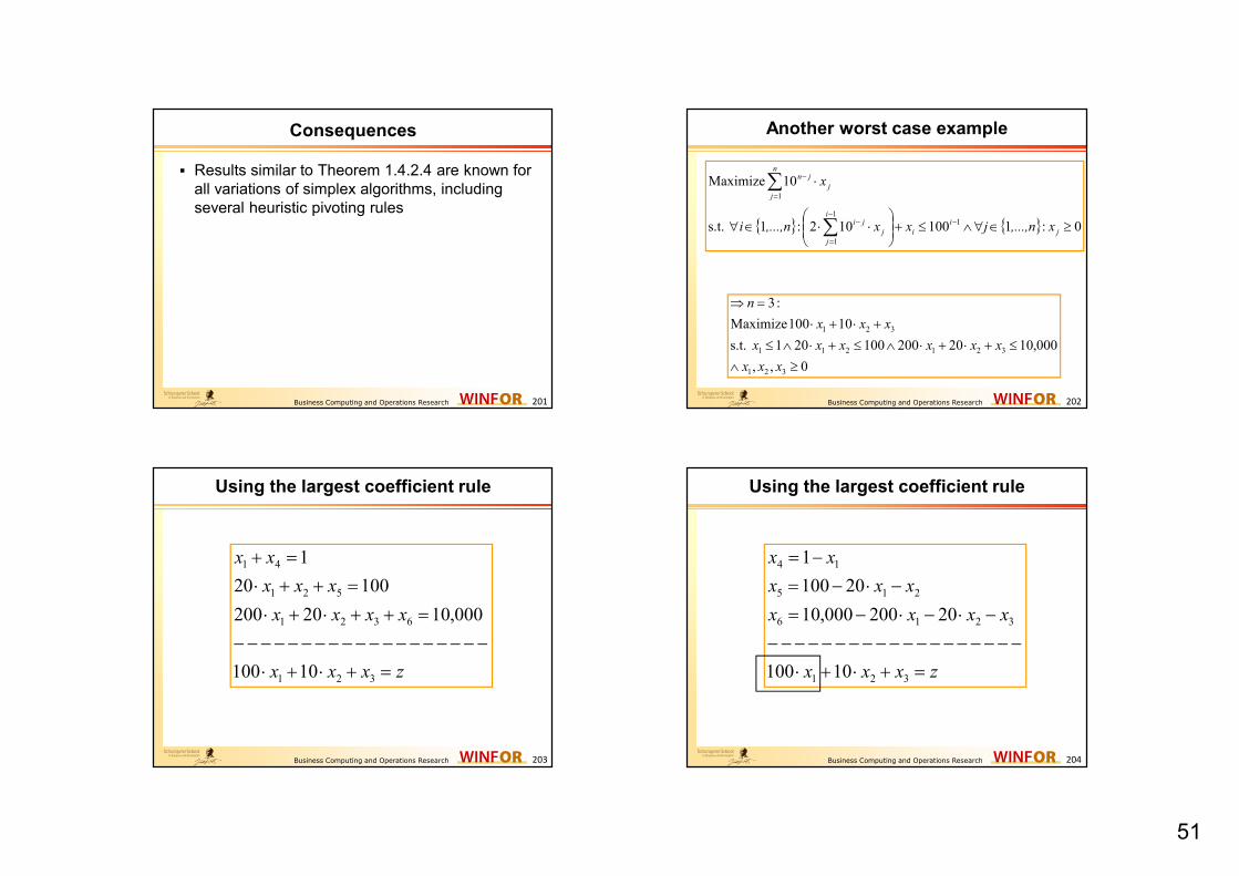
51
Business Computing and Operations Research 201
Consequences
� Results similar to Theorem 1.4.2.4 are known for all variations of simplex algorithms, including several heuristic pivoting rules
Business Computing and Operations Research 202
Another worst case example
{ } { } 0:1100102:1 s.t.
10 Maximize
11
1
1
≥∈∀∧≤+
⋅⋅∈∀
⋅
−−
=
−
=
−
∑
∑
j
i
i
i
j
j
ji
n
j
j
jn
x,...,njxx,...,ni
x
0,,
000,1020200100201 s.t.
10100 Maximize
:3
321
321211
321
≥∧
≤+⋅+⋅∧≤+⋅∧≤
+⋅+⋅
=⇒
xxx
xxxxxx
xxx
n
Business Computing and Operations Research 203
Using the largest coefficient rule
zxxx
xxxx
xxx
xx
=+⋅+⋅
−−−−−−−−−−−−−−−−−−−
=++⋅+⋅
=++⋅
=+
321
6321
521
41
10100
000,1020200
10020
1
Business Computing and Operations Research 204
Using the largest coefficient rule
zxxx
xxxx
xxx
xx
=+⋅+⋅
−−−−−−−−−−−−−−−−−−−
−⋅−⋅−=
−⋅−=
−=
321
3216
215
14
10100
20200000,10
20100
1

52
Business Computing and Operations Research 205
Using the largest coefficient rule
1 4
5 4 2
6 4 2 3
4 2 3
1
80 20
9,800 200 20
100 100 10
x x
x x x
x x x x
x x x z
= −
= + ⋅ −
= + ⋅ − ⋅ −
− − − − − − − − − − − − − − − − − − −
− ⋅ + ⋅ + =
Iteration 1
Business Computing and Operations Research 206
Using the largest coefficient rule
zxxx
xxxx
xxx
xx
=+⋅−⋅+
−−−−−−−−−−−−−−−−−−−
−⋅+⋅−=
−⋅+=
−=
354
3546
542
41
10100900
20200200,8
2080
1
Iteration 2
Business Computing and Operations Research 207
Using the largest coefficient rule
zxxx
xxxx
xxx
xx
=+⋅−⋅−
−−−−−−−−−−−−−−−−−−−
−⋅+⋅+=
−⋅−=
−=
351
3516
512
14
10100000,1
20200000,8
20100
1
Iteration 3
Business Computing and Operations Research 208
Using the largest coefficient rule
4 1
2 1 5
3 1 5 6
1 5 6
1
100 20
8 000 200 20
9 000 100 10
x x
x x x
x , x x x
, x x x z
= −
= − ⋅ −
= + ⋅ + ⋅ −
− − − − − − −− −− − −− −− − −− −
+ ⋅ + ⋅ − =
Iteration 4

53
Business Computing and Operations Research 209
Using the largest coefficient rule
1 4
2 4 5
3 4 5 6
4 5 6
1
80 20
8 200 200 20
9 100 100 10
x x
x x x
x , x x x
, x x x z
= −
= + ⋅ −
= − ⋅ + ⋅ −
− − − −− − −− −− − −− −− − −− −
− ⋅ + ⋅ − =
Iteration 5
Business Computing and Operations Research 210
Using the largest coefficient rule
zxxx
xxxx
xxx
xx
=−⋅−⋅+
−−−−−−−−−−−−−−−−−−−
−⋅−⋅+=
−⋅+=
−=
624
6243
245
41
10100900,9
20200800,9
2080
1
Iteration 6
Business Computing and Operations Research 211
Using the largest coefficient rule
solution! Optimal
10100000,10
20200000,10
20100
1
621
6213
215
14
⇒
=−⋅−⋅−
−−−−−−−−−−−−−−−−−−−
−⋅−⋅−=
−⋅−=
−=
zxxx
xxxx
xxx
xx
Iteration 7
Business Computing and Operations Research 212
Assessing this calculation
Hmmmpffff!For solving this tiny problem, we
have conducted 7 iterations!
Hmmmpffff!For solving this tiny problem, we
have conducted 7 iterations!
Moreover, we were quite stupid. If we had applied the largest improvement
rule, we would have succeeded in just a single
iteration!!

54
Business Computing and Operations Research 213
Largest improvement rule
{ }
4 1
5 1 2
6 1 2 3
1 2 3
1
1
100 20
10,000 200 20
100 10
1,..., : 0 : Improvement min 0, 1,...,
100 10,000min 1, , min 1,5,50 1 Improvem
20 200
ij j j ij
ij
x x
x x x
x x x x
x x x z
bj n c c a i m
a
x
= −
= − ⋅ −
= − ⋅ − ⋅ −
− − −− −− − −− −− −− − −− −− −
⋅ + ⋅ + =
∀ = > = ⋅ < = −
⇒ ≤ = = ⇒
{ }
{ }
1
2 2
3 3
3
ent = 100
10,000min 100, min 100,500 100 Improvement = 1,000
20
min 10,000 10,000 Improvement = 10,000
Choose the variable with the largest improvement
x
x
x
≤ = = ⇒
≤ = ⇒
⇒
Business Computing and Operations Research 214
Largest improvement rule
solution! Optimal
10100000,10
20200000,10
20100
1
621
6213
215
14
⇒
=−⋅−⋅−
−−−−−−−−−−−−−−−−−−−
−⋅−⋅−=
−⋅−=
−=
zxxx
xxxx
xxx
xx
Iteration 1
Business Computing and Operations Research 215
Alternative pivoting rules
� Two efficiency aspects to be considered for assessing pivoting rules� Number of iterations that are induced by the application of the rule� Effort of each iteration
� Generally, it can be stated that the number of iterations required by the largest improvement rule is usually smaller than the number of iterations caused by the largest coefficient rule
� This was underlined empirically� However, the costs caused by each iteration are
increased by the largest improvement rule� Nevertheless, in a direct comparison the reduced number
of iterations prevails and therefore the largest improvement rule outperforms the largest coefficient rule
Business Computing and Operations Research 216
Attention
� However, as already mentioned, each rule has its own specific worst case scenario
� Thus, according to worst case considerations, there is no real distinction between different pivoting rules
� In modern software packages, pivoting rules are chosen according to the handling of large sized problems on a computer
� However, it can be shown that LP is polynomiallysolvable. But this is done by using a different solution strategy

55
Business Computing and Operations Research 217
Complexity of Linear Programming
� Until 1979, the open question whether there can be any polynomial-time algorithm for LP was a most perplexing question (Papadimitriou and Steiglitz (1982,1988), p.170)
� Specifically, there was conflicting evidence about the possible answer � On the one hand, LP was certainly one of the problems (together with
the TSP and many others) which seemed to defy all reasonable attempts at the development of a polynomial-time algorithm.
� However, on the other hand, LP had two positive features that made it completely different from the other classical hard problems � First, LP has a strong duality theory, which is conspicuously lacking for
all the other hard combinatorial problems
� Secondly, LP has an algorithm, the simplex method, which – although exponential in its worst case – certainly works empirically on instances of seemingly unlimited size.
Business Computing and Operations Research 218
Complexity of Linear Programming
� In the spring of 1979 the Soviet mathematician L.G. Khachian proposed an exact polynomial-time solution algorithm for LP (see the paper of Khachian, L. G. (1979)), the so-called ellipsoid algorithm
� Therefore, it was proven that LP is well solvable (in the language of the Complexity Theory), i.e., 2& ∈ &
� This important work was assessed, evaluated and further extended by the papers of Aspvall and Stone (1980), Dantzig, G.B. (1979), and Goldfarb, D., Todd, M.J. (1980)
Business Computing and Operations Research 219
Performance of the ellipsoid algorithm
� Despite the great theoretical value of the ellipsoid algorithm (for worst case scenarios), this algorithm seems to be not very useful in practice� The most obvious among many obstacles is the large
precision that is required by the conducted computations
� Hence, average running times are not competitive, i.e., it is outperformed by the Simplex algorithm for real-world problems
Business Computing and Operations Research 220
Interior point methods
� In 1984, however, Karmarkar, N. (1984) proposes a further polynomial exact solution algorithm for Linear Programming
� In contrast to the Simplex algorithm that moves from edge point to edge point, this procedure finds an optimal solution by iteratively moving through the interior of the solution space until optimality was proven
� Interior methods are also very efficient in practice and are competitive with the Simplex algorithm� This applies in particular to LP with sparsely populated matrices
� However, the Simplex algorithm is superior if a series of problems has to be solved (e.g., applied as a subroutine within a Branch&Bound algorithm for integer problems)

56
Business Computing and Operations Research 221
1.5 How to work with tableaus
� In order to provide a direct understanding of the Simplex procedure, we have illustrated its calculations on the basis of dictionaries
� However, in what follows, we make use of tableaus
� Tableaus are directly derived from the use of matrices in order to solve Linear Programs
� By making use of them, we are able to illustrate several aspects of the matrix transformations executed during the conduction of the Simplex procedure
� Moreover, matrix operations play a crucial role for implementing the Simplex Method as efficiently as possible
� This is done by the so called Revised Simplex Method
Business Computing and Operations Research 222
1.5.1 Basis change
0
0 0 1 0
0
0
0
Consider a basic feasible solution , with 0
and additionally a feasible solution with . Furthermore, let
with 0 and it holds: .
Then, since 0, it
B
B B N
N
n
N
xx x A b x
x
x A x b
y IR A y x x y
x
− = = ⋅ ∧ =
⋅ =
∈ ⋅ = = +
=
1 1
1
1 1
obviously holds: .
Additionally, we derive:
0 0
0 .
We define the basis vectors by and the remaining vect
N N
B B N N B B B B N N
B N N
B B N N B B N N
N
x y
A y A y A x A A y A A x
A A xy A A x y A A x y
x
B
− −
−− −
=
= ⋅ = ⋅ + ⋅ ⇒ = ⋅ ⋅ + ⋅ ⋅
− ⋅ ⋅⇒ = + ⋅ ⋅ ⇒ = − ⋅ ⋅ ⇒ =
ors by .N
Business Computing and Operations Research 223
Basis change
( ) ( )
1
1
1 1 1 1
In the following, we introduce the component in the basis.
We introduce the shortcut ,
with , ,..., ,..., , with .
Note that
−
−
− × −
−
− ⋅ ⋅ = =
= ⋅
∈ = = ⋅ ∈
B B N N
N N
B
m m n n j m
B B
B
y A A xy
y x
t
A A A
A IR A a a A a a a IR
A
�0
0
1
Position
.
Let us now set: 0,...,0, 1 ,0,....,0 .
× × ×
−
∈ ∧ ∈ ⇒ ∈
= = ∈
m m m n m n
T
k n m
N
k
IR A IR A IR
x e IR
Business Computing and Operations Research 224
Basis change
( )
( )
( )( ) 000
000
1
0
0
0
0
0
0Let
:case in this followsit Thus,
.column basic-nonth therepresentsmatrix original
in thecolumn th theI.e., . assume wee,Furthermor
xe
axyyx
bbyAxAyxAyxx
e
a
y
yyaxAAy
k
tkNt
k
t
B
k
t
B
N
Bt
NNBB
−≥
−⋅⇔−≥⋅⇔≥⋅+
=+=⋅⋅+⋅=⋅+⋅⇒⋅+=
−=
=⇒−=⋅⋅−=
=
−
λλλ
λλλλ

57
Business Computing and Operations Research 225
Conducting a basis change
( ) ( ) ( )
( )
0 0
0
0
0
,
0
min | 0 if : 0
0 otherwise
Note that 0 is feasible for these values of . Let us consider the
result of our calc
t t
B B B
k k
B j t t
t j j
j
λ
a x a
x
e e
x
a j aa
x λ
λλ
λ
λ
− − ⋅ ⋅ ≥ − ⇔ ≥ ⇒ ⋅
> ∃ >
= ≥
≥
( ) ( )
( ) ( )
0
0
, if 0
...ulations: , i.e., if
0 otherwise
...
0
t
B B
t
iB j
λ
j
x a
x λ a B i j
x x λ j tλ
λ
λ
− ⋅
− ⋅ = = = =
Business Computing and Operations Research 226
Observation
� By setting λ to a maximal feasible value, we erase the corresponding variable out of the basis and introduce the tth entry instead
� In the following, we examine a simple example
Business Computing and Operations Research 227
Basis change – An illustrative example I
( )
( ) ( ) ( ) 43,32,21set ,
5
12
10
10012
01043
00152
3020,Min
5323 have We
512
1243
1052
25050100
600200150
500250100
===
=∧
−
−
−
=
⋅+⋅=
=+=∧=
≥⋅+⋅
≥⋅+⋅
≥⋅+⋅
⇔
≥⋅+⋅
≥⋅+⋅
≥⋅+⋅
BBBbA
babaf
nm
ba
ba
ba
ba
ba
ba
Business Computing and Operations Research 228
( ) ( ) ( )
=⋅∧
−
−
−
=⋅⇒
−
−=⇒
−
−
=
===
=∧
−
−
−
=
−−
−
8
15
5
41005
50108
10012
410
501
100
001
104
015
43,32,21set ,
5
12
10
10012
01043
00152
11
1
bAAA
AA
BBBbA
BB
BB
Basis change – An illustrative example II

58
Business Computing and Operations Research 229
( )
( ) ( ) ( )
We introduce column , i.e.,
min , ,
and obtain , ,
t
B
k
t
ax x
e
B B B
λλ λ
=
− ⇒ = = ⇒ = + ⋅
− = + ⋅ = = = =− −
0
0
1 1
5 15 8 8
2 8 5 5
8
50 1
95 2
581 2 2 3 3 115 8
1158 5
5
0 0 0
0
Basis change – An illustrative example III
Business Computing and Operations Research 230
( ) ( ) ( )
1
1 1
2 5 1 0 0 10
3 4 0 1 0 12 , set 1 2, 2 3, 3 4
2 1 0 0 1 5
5 1 0 0 0 1
4 0 1 1 0 5
1 0 0 0 1 4
2 1 0 0 1 5
8 0 1 0 5 15
5 0 0 1 4 8
Instead of introducing
B B
B B
A b B B B
A A
A A A b
−
− −
− = − ∧ = = = = −
− = − ⇒ = − −
− ⇒ ⋅ = − ∧ ⋅ = −
column 1, now, we try column 5, i.e., 5t =
Basis change – An illustrative example IV
Business Computing and Operations Research 231
( )
0
5
0
Thus, we obtain:
1
5 0
4
0 0 0
5 1 5
0 15 5 15 5
8 4 8 4
0 1
and yield a ray.
t
B
k
a
ax x
e
λλ
λ λ λ λλ
λ
− ⇒ = − < −
+ −
⇒ ≥ ⇒ = + ⋅ = + ⋅ = + ⋅ + ⋅
Basis change – An illustrative example V
Business Computing and Operations Research 232
Direct consequences
1.5.2 Theorem
( ) ( )
{ } { }
0
00
0
0
0
1. If there exists an with 0, then min | 0 ,
and is a basic feasible solution (bfs) of . Basis
is B/ .
2. If 0, then with ,
B iB it t
i it t
i i
Bt t
B
N
xxi a a
a a
x x x y P
i t
ya y y a
y
λ
λ
λ
> = > =
= = + ⋅
∪
≤ = = −
ɶ
ɶ
ɶ
0
0
and greater equal 0
and, therefore, it holds: , 0
k
Ny e
x x y Pλ λ λ
=
= + ⋅ ∈ ∀ ≥

59
Business Computing and Operations Research 233
Proof of Theorem 1.5.2
( )( )( ){ }( )
( )
( )
0
0
1
if 1. Define by .
otherwise
1,..., :
0 0
Since 0 , .
We replace by in the basis. Thus, arises.
.
is basic feasible solu
j N
t t t t t
i B B
N i i iN N i
B i
x x y j N n m
x x
a a A a a A a
B i t B
A x b
x
λ
−
≠=
⇒ = + ⋅ ⇒∀ ∈ −
= ⇒ =
> ⇒ = ⋅ = ⋅
⋅ =
⇒
ɶ
ɶ
ɶ
tion for .
2. trivial
P
Business Computing and Operations Research 234
Kinds of degeneration
� Primal degeneration of x0:
If λ0=0, then one basic variable equals zero. The objective function value is kept unchanged
0
1
2
3
4
5
6
0 1 2 3 4 5 6 7 8 9 10
x[1]
x[2
]
1 2
1 2
2
1
1 2
7
. . 5
2
3
, 0
Maximize x x
s t x x
x
x
x x
+
+ ≤
≤
≤
≥
Business Computing and Operations Research 235
Observation
� Consider the example� We have five variables altogether (two structure
variables and three slack variables)
� Since m=3, we have always three basic variables
� Clearly, one slack variable becomes zero in the optimal solution
� Note that this is not restricted to optimal solutions
Business Computing and Operations Research 236
Kinds of degeneration
� Dual degeneration of x0:
If for one non-basic variable the relative costs are zero, we are facing a constellation of dual degeneration, i.e., all solutions integrating this variable into the basis yield the same objective function value
0
1
2
3
0 1 2 3 4 5 6 7 8 9 10
x[1]
x[2
]
1 2
1 2
1 2
1 2
3
. . 2 5
2 6 12
, 0
Maximize x x
s t x x
x x
x x
+
+ ≤
+ ≤
≥

60
Business Computing and Operations Research 237
Neighboring basic feasible solution
1.5.3 Definition
Two basic feasible solutions that can be mutually transformed in each other by changing a single basis vector are denoted as neighboring basic feasible solutions.
Business Computing and Operations Research 238
Basis change and objective function value
0
0 0 1 0
0
0 1
0
Let , with , 0 a basic feasible solution.
Assuming it holds: ,
for with .
We calculate:
B
B B N
N
B B
B B N N
N N
N N
T T T T
B B N N
T
xx x A b x
x
x yx x y A A x
x y
y x x A x b
c x c x c y c y
c
−
−
= = ⋅ =
= = + = − ⋅ ⋅ ∧
= ⋅ =
⋅ = ⋅ + ⋅ + ⋅
= ⋅
( )
0 1
0 1
0 1
T T
B B N N N N
T T T
B B N N N N
T T T
N B B N N
x c A A x c y
c x c A A x c x
c x c c A A x
−
−
−
− ⋅ ⋅ ⋅ + ⋅
= ⋅ − ⋅ ⋅ ⋅ + ⋅
= ⋅ + − ⋅ ⋅ ⋅
Business Computing and Operations Research 239
( )( )
( )NB
T
B
T
N
T
BBB
T
BBB
T
B
T
B
N
T
N
T
N
T
NNB
T
B
T
N
T
TT
B
T
B
T
AAcz
cAAcAAcz
xzcxc
xAAccxc
AπzAcπ
⋅⋅=∧
=⋅⋅=⋅⋅=⇒
⋅−+⋅=
⋅⋅⋅−+⋅⇒
⋅=⋅=
−
−−
−
−
1
11
0
10
1 and introduce We
Substitution
Business Computing and Operations Research 240
( ) ( )0 0
0
0
Altogether, we get
.
Thus,
defines the change
(or reduced costs/prices) when is transformed into .
Specifically, it holds:
T T T T T T T
N N N
T T T
T T T
c x c x c z x c x c z x
c c z
x x
c x c x c x
⋅ = ⋅ + − ⋅ = ⋅ + − ⋅
= −
⋅ = ⋅ + ⋅
relative costs
.
Relative cost change

61
Business Computing and Operations Research 241
Optimality criterion
1.5.4 Theorem
0
0
1. By moving between neighboring basic feasible
solutions as introduced above, the objective function
value is modified by .
2. If 0, then is an optimal solution for a
minimization problem.
N
tc
c x
λ⋅
≥
ote that 0 is the optimality criterion for maximization
problems.
c ≤
Business Computing and Operations Research 242
Proof of Theorem 1.5.4
( ) ( )
( )
0 00 0
1
1. Calculate
, since ,
2. Consider an arbitrary solution and a minimization problem
0
We assume 0 0
−
⋅ = ⋅ + − ⋅ = ⋅ + ⋅ = ⋅ =
∈
⇒ ⋅ = ∧ ≥ ⇒ ⋅ = ⋅ + ⋅ − ⋅
≥ ⇒ ⋅ − ⋅ ≥
≥ ⋅ = ⋅ ⋅
T T T T T kN N N t N
T T T T
T T
T T
B B
c x c x c z x c x c x e N k t
x P
A x b x c x c x z x z x
c c x z x
z x c A
λ λ
0 0 0 0
0 0 0
0 0
0
0 : is optimal
⋅ = ⋅ ⋅ = ⋅
= ⋅ ⋅ = ⋅ = ⋅ + ⋅
= ⋅ + = ⋅ = ⋅
⇒ ≥ ⇒∀ ∈ ⋅ ≥ ⋅ ⇒
T T
T T T TB B N N
T T T
B B B B
T T
A x π A x π b
π A x z x z x z x
z x c x c x
c x P c x c x x
Business Computing and Operations Research 243
Summary
( ) 0
Assuming an LP Problem is given in standard form,
i.e., minimize with respect to 0 .
Furthermore, we assume and that is a
basic feasible solution (bfs).
We are transforming the p
Tc x x A x b
rank A m x
⋅ ≥ ∧ ⋅ =
=
( ) ( )
1
1
1
roblem by . Denote as
an elementary matrix.
We introduce
0, and .
B m
B B N m N
T T T
B B
A E
m×m
A A A A ,A E , A ,
b A b x c c π A
−
−
−
= ⋅ = =
= ⋅ = ≥ = − ⋅
Business Computing and Operations Research 244
Summary
( )( ) ( )
( ) ( )
1
1 1
1
0 0
By multiplying , we get the following equivalent problem:
Minimize , s.t.
B
T
B B
T T T T T T T
T T T T T T
B B
T T T T T T
A
c x A A x A b A x b
c x c x z x z x c z x z x
c z x c A A x π b c z x
π A x c z x z x c z x
−
− −
−
⋅ ⋅ ⋅ = ⋅ ⇔ ⋅ =
⋅ = ⋅ + ⋅ − ⋅ = − ⋅ + ⋅
= − ⋅ + ⋅ ⋅ ⋅ = ⋅ + − ⋅
= ⋅ ⋅ + − ⋅ = ⋅ + − ⋅
= ( ) ( )( ) ( )
0 0 0
0 0 0
0T T T T T T T
B B N N B B
T T T T T T T T
B B
z x z x c z x z x c z x
c x c z x c x c z x c x c x
⋅ + ⋅ + − ⋅ = ⋅ + + − ⋅
= ⋅ + − ⋅ = ⋅ + − ⋅ = ⋅ + ⋅

62
Business Computing and Operations Research 245
3 Cases may occur
( )
0
1 1 0
1 0
0
1. 0 is an optimal solution to
2. 0 0 The objective function is not bounded
against
3. 0 0
If 0 it holds
Note that there are constellatio
t
t
t T T
t j
T T
c x P
t : c a
t : j : c a x ε P : c x c x .
λ c x c x
≥ ⇒
∃ < ∧ ≤ ⇒
∞
∃ ∃ < ∧ > ⇒ ∃ ∈ ⋅ ≤ ⋅
> ⋅ < ⋅
ns possible where cases 2 and 3
apply, simultaneously. Furthermore, it is worth mentioning that
all results are directly derived from Theorem 1.5.4.
Business Computing and Operations Research 246
1.5.5 The Tableau
� In order to obtain a basic feasible solution, the following transformation is conducted
� This is illustrated by the following tableaus� Specifically, the modifications are stepwise done by
ordinary row transformations, i.e., we produce the matrix Em out of A and 0 out of cT for the basis vectors of AB
-1.A
0 cT
b A
-cTx0 cT = cT-cBT.AB
-1.A= cT-zT
b = AB-1.b A = AB
-1.A
Business Computing and Operations Research 247
The Primal Simplex Algorithm
1. Transform the primal problem into canonical form, generate equations and a minimization objective function.
2. Initialization with a feasible basic solution to the primal problem.
3. Are there strictly negative cost coefficients in the current solution?
“Yes”: Iteration
� Pivot column t:- Largest coefficient rule
- Smallest subscript rule
- Largest improvement rule
� If , then terminate since the solution space is unbounded.
� Pivot row s: that is an upper bound on xt.
� Basis change: xt enters the basis and xB(s) becomes a non-basic variable.
Apply a linear transformation of the constraint equalities by the Gauß-Jordan algorithm to yield a unit vector with ast=1 at the pivot element (i.e., es in column t). Go to step 3.
“No”: Termination. An optimal basic solution to the primal problem is found.
{ }min 1,..., 0j
j n c= <
{ }min 0 1,...,j
c j n< ∀ =
{ }min / 1,..., : 0i it it
b a i m a∀ = >
max min : 0 : 0ij ij j
ij
bc i a j c
a
⋅ ∀ > ∀ <
c
0 1,...,it
a i m≤ ∀ =
Business Computing and Operations Research 248
Calculation with tableaus – Example I.I
1 2 3
1 2 3
1 2 3
1 2 3
1 2 3
Consider the example from the calculation with dictionaries.
Max 5 4 3
s.t. 2 3 1 5
4 1 2 11
3 4 2 8
, , 0
Introducing the slack variabl
x x x z
x x x
x x x
x x x
x x x
⋅ + ⋅ + ⋅ =
⋅ + ⋅ + ⋅ ≤
⋅ + ⋅ + ⋅ ≤
⋅ + ⋅ + ⋅ ≤
≥
4 5 6
1 2 3 4 5 6
1 2 3 4 5 6
1 2 3 4 5 6
1 2 3 4 5 6
es , , , we transform the problem.
Min 5 4 3 0 0 0
s.t. 2 3 1 1 0 0 5
4 1 2 0 1 0 11
3 4 2 0 0 1 8
x x x
x x x x x x z
x x x x x x
x x x x x x
x x x x x x
− ⋅ − ⋅ − ⋅ + ⋅ + ⋅ + ⋅ = −
⋅ + ⋅ + ⋅ + ⋅ + ⋅ + ⋅ =
⋅ + ⋅ + ⋅ + ⋅ + ⋅ + ⋅ =
⋅ + ⋅ + ⋅ + ⋅ + ⋅ + ⋅ =
1 2 3 4 5 6 , , , , , 0x x x x x x ≥

63
Business Computing and Operations Research 249
Calculation with tableaus – Example I.II
( ) ( ) ( )
3
We commence with the basis 1 4 2 5 3 6
1 0 0
0 1 0 . The trivial initial solution is feasible,
0 0 1
and the start tableau is as follows :
0
0 5 4 3 0 0 0 0
5 2 3 1 1 0 0 0
11 4 1 2 0 1 0 5
8 3 4 2 0 0 1 11
8
B
B B B
A E
x
= ∧ = ∧ =
⇒ = =
− − −
⇒ =
( ) 5, 4, 3,0,0,0TP c
∈ = − − −
Business Computing and Operations Research 250
Calculation with tableaus – Example I.III
{ }
( )
0 1
Applying the largest coefficient rule, a further improvement is possible.
We try to introduce 1 into the basis
5 8 5111 since min , ,2 4 3 2
25 7 510 0 02 2 2 20 5 4 3 0 0 0
5 3 1 11 0 05 2 3 1 1 0 02 2 2 2
11 4 1 2 0 1 0 1
8 3 4 2 0 0 1
t
t
i a
=
⇒ = = =
−− − −
⇒
( ) ( )
52
12
40 5 0 2 1 0
231 1 1 30 0 1
2 2 2 2 2
5 7 5 251 1,0,0,0,1, 0, , , , 0,0 2 2 2 2 2 2
T Tx P c z
⋅
⋅
⋅−− −
− − ⋅−
⇒ = ∈ = − =
Business Computing and Operations Research 251
Calculation with tableaus – Example I.IV
{ }
( )( )
0 3
Further improvement is possible. We try to introduce 3 into the basis
3 since min 5,1 1
25 7 510 0 02 2 2 2 13 0 3 0 1 0 1 1
5 3 1 11 0 0 2 1 2 0 2 0 1 12 2 2 2 1 0 5 0 2 1 01 0 5 0 2 1 0
1 0 1 1 3 0 2 231 1 10 0 12 2 2 2
2,0,1,0,1,0
t
T
t
i a
x
=
⇒ = = =
−⋅
− ⋅−⇒
− −− −− − ⋅− −
⇒ = ( )
( ) ( ) ( )4 5 6 3
0,3,0,1,0,1 13
Since 0, the solution is optimal and the total costs are 13.
Furthermore, , , 0,0,0 1,0,1 .
T
T
T T
P c z
c z c x
c c c π E π
∈ = =
⇒ ≥ = ⋅ =
= − ⋅ = =
Business Computing and Operations Research 252
Calculation with tableaus – Example II.I
( ) ( )
1 2 3 4 1 2 3 4
1 2 3
1 2 3 4
We consider the following example:
Minimize 2 3 0 with 0
with subject to the restrictions
5
2 3 9
2
We commence with the basis
1 11 1 2 2
2 1B
x x x x x ,x ,x ,x
x x x
x x x x
m
B B A
⋅ + ⋅ + + ⋅ ≥
+ + =
⋅ + + ⋅ − =
⇒ =
= ∧ = ⇒ =

64
Business Computing and Operations Research 253
Px ∈
=⇒
−
−
−−
⇒
−
−
−−
⇒
−
−−
⇒
−−−
−−
⇒
−
0
0
1
4
11101
12014
100011
11101
12014
011010
11101
01115
011010
11101
01115
011010
13129
01115
01320
Calculation with tableaus – Example II.II
Business Computing and Operations Research 254
( )
( )
0 1 2
411 0 0 0 1
14 1 0 2 1 0,0,0, 1
01 0 1 1 1
0
Further improvement is possible
We try to introduce 4 in the basis 2 since 1 0 1
11 0 0 0 1 10 0 1 1 0
4 1 0 2 1 5 1 1 1 0
1 0 1 1 1 1 0 1 1 1
5
0
0
1
T
t t
x P c
t i a a
x
− −
− ⇒ = ∈ = −
−
⇒
= ⇒ = = − < ∧ =
− − − −
− ⇒
− −
⇒ =
( ) 0,1, 1,0T
P c
∈ = −
Calculation with tableaus – Example II.III
Business Computing and Operations Research 255
( )
( )
0 2 1
Further improvement is possible. We try to introduce
3 in the basis 1 since 1 0 1
10 0 1 1 0 5 1 2 0 0
5 1 1 1 0 5 1 1 1 0
1 0 1 1 1 6 1 2 0 1
0
0 1,2,0,0
5
6
Optimal solution with total costs
t t
T
t i a a
x P c
⇒
= ⇒ = = − < ∧ =
− − −
⇒
−
⇒ = ∈ =
⇒ 5TZ c x= ⋅ =
Calculation with tableaus – Example II.IV
Business Computing and Operations Research 256
Additional literature to Section 1
� Aspvall, B. and Stone, R.E. (1980): "Khachiyan's Linear Programming Algorithm,“ Journal of Algorithms 1, no. 1.
Anticycling rule:
� Bland, R. G. (1976): "New Finite Pivoting Rules," Discussion Paper 7612, Center for Operations Research and Econometrics (CORE), Universite Catholique de Louvain, Heverlee, Belgium, June 1976 (revised January 1977).
The first publication of the simplex algorithm was:
� Dantzig, G.B. (1949, 1951): "Programming of Interdependent Activities, H, Mathematical Model," pp. 19-32, in Koopmans, T.C. (ed.): Activity Analysis of Production and Allocation. John Wiley & Sons, Inc., New York. Also in Econometrics 17, nos. 3 and 4 (July-Oct. 1949), 200-211.
� Dantzig, G.B. (1951): Maximization of a linear function of variables subject to linear inequalities. In: Activity Analysis of Production and Allocation (T.C. Koopmans, ed.), Wiley, New York, pp. 359–373

65
Business Computing and Operations Research 257
Additional literature to Section 1
� Dantzig, G.B. (1963): Linear Programming and Extensions. Princeton, N.J.: Princeton University Press.
� Dantzig, G.B. (1979): Comments on Khachian's Algorithm for Linear Programming. Technical Report SOL 79-22, Dept. of Operations Research, Stanford University.
� Goldfarb, D., Todd, M.J. (1980): Modifications and Implementation of the Schor-Khachian Algorithm for Linear Programming. Department of Computer Science, Cornell University.
� Grünbaum B. (1967): Convex Polytopes. John Wiley & Sons, Inc., New York.
� Karmarkar, N. (1984): A new polynomial-time algorithm for Linear Programming. Combinatorica 4(4), pp. 373-395.
� Khachian, L. G. (1979): A Polynomial Algorithm for Linear Programming,“ Doklady Akad. Nauk USSR, 244, no. 5 (1979), 1093-96. Translated in Soviet Math. Doklady, 20, 191-94.
Business Computing and Operations Research 258
Additional literature to Section 1
� Klee, V., Minty, G.J. (1972): How Good is the Simplex Algorithm? Inequalities III, edited by O. Shisha. New York: Academic Press, Inc, pp.159-175.
� Kuhn, H. W. (1976): Class Notes, Princeton University, 1976.
� Rockafellar, R.T. (1970): Convex Analysis. University Press, Princeton, N.J.
Dantzig (1961) attributes the formulation of the diet problem to
� Stigler, G.J. (1945): "The Cost of Subsistence," J. Farm Econ., 27, no. 2 (May 1945), pp. 303-314.