Embed Size (px)
Citation preview

Colour Appearance Issues in Digital Video, HD/UHD, and D‑cinema
Charles Poynton B. A., Queen’s University, 1976
Thesis Submitted in Partial Fulfillment of the Requirements for the Degree of Doctor of Philosophy
Under Special Arrangements with Graduate and Postdoctoral Studies and Faculty of Applied Sciences
© Charles Poynton 2018 Simon Fraser University Summer 2018 Copyright in this work rests with the author. Please ensure that reproduction or re-use accords with relevant copyright regulations.

Approvals
Charles Poynton
for the degree of
Colour Appearance Issues in Digital Video, HD/UHD, and D‑cinema
Doctor of Philosophy
Chair:
Examining committee
Binay Bhattacharya Professor, Computing Science
Senior supervisor:
Brian Funt Professor, Computing Science
Supervisor:
Mark Drew Professor, Computing Science
Supervisor:
Kathleen Akins Professor, Philosophy
Examiner:
Lyn Bartram Associate Professor, School of Interactive Arts and Technology
External examiner:
Michael S. Brown Professor, EECS York University, Toronto
Date Defended/Approved Date of this version
2018-07-30 2019-10-05
ii

iii
Abstract
For many decades, professional digital imaging has faced a dilemma. On one hand, imaging scientists and engineers – and, within the last two decades, programmers – have been taught that the goal of imag-ing technology is the accurate “reproduction” of colour values (most commonly quantified by luminance, tristimuli, and/or chromaticity) on a display device. On the other hand, digital imaging craftspeople and artists have learned to manipulate image data as required to yield the intended visual result, objective inaccuracy notwithstanding.
These approaches have been at odds owing to a fundamental aspect of colour vision: Colour appearance depends upon the visual conditions of a scene or a display (particularly, its absolute illuminance or lumi-nance), the region surrounding the acquired portion of the scene or the displayed image, and whether the display is emissive or reflective. The dependence of perceived colour upon absolute luminance and sur-round conditions is well known in colour science. In the last 20 years, these visual effects have been quantified in colour appearance models, and have been standardized (in CIECAM02). However, these effects, and colour appearance theory, remain largely unknown to imaging engineers.
Despite the reluctance of scientists and engineers to abandon their goal of physical accuracy, appearance effects have, in fact, been accommodated in commercially important imaging systems. However, appearance effects have been compensated largely at the level of craft, not science or engineering. Compensation of appearance effects has been subject to such confusing nomenclature and such poor documen-tation that it has remained mostly invisible or mysterious to the scien-tists and engineers.
This thesis seeks to develop a systematic analysis that bridges visual psychophysics, colour appearance theory, and the practice of image sig-nal processing in modern digital imaging systems. I analyze and docu-ment the colour appearance compensation methods that have evolved in modern digital imaging, and I link to these methods to modern psychovisual principles and to colour appearance theory.

iv

v
dedicated to
Alexander Johnston 1839 –1896
artist and photographer Wick, Caithness Scotland
and
Alexander Johnston 1920 –1989
rangeland ecologist, research scientist, and historian Lethbridge, Alberta Canada

vi

vii
Acknowledgements
Thanks to my supervisor Brian Funt, who waited much longer than he anticipated, even taking into account Hofstadter’s Law.
Thanks to my other two supervisory committee members, Kathleen Akins and Mark Drew, for agreeing to participate in what – even at the outset – promised to be an unconventional PhD programme. Thanks to my examiners for their thoughtful comments.
Thanks to the faculty members at other institutions who helped in various ways: Mark Fairchild, Richard Hornsey, Sabine Susstrunk, and 為ヶ谷 秀一 (Tamegaya, Hideichi).
I thank Michael Brill for teaching me, 15 years ago, the vital importance of distinguishing absolute and relative luminance, and of using the correct letter symbols. And for writing a poem about me.
I acknowledge four colleagues-turned-friends who offered me encouragement in the early stages but sadly are no longer with us; I think they would have enjoyed the result: Dick Shoup, Lou Silverstein, Jim Whittlesey, and Lance Williams.
I formulated many of the ideas expressed here while teaching. Thanks to my long-time collaborators in that effort: Katrin Richthofer and Peter Slansky at HFF Munich; and Dirk Meier, Edmond Laccon, and all of the UP.GRADErs at DFFB Berlin.
Thanks to my personal network of colleague/friend reviewers, who provided valuable criticism – some, quite harsh! – and literally hundreds of suggestions and corrections, all taking time to help me while pursuing their own dreams: Don Craig, Dave LeHoty, Barry Medoff, Katherine Frances Nagels, Julia Röstel, Mark Schubin, Jeroen Stessen, 菅原正幸 (Sugawara, Masayuki), and Louise Temmesfeld.
Thanks to my friends, who provided companionship, advice, encouragement, coffee, and other necessities; especially: Marianne Apostolides, Jan Fröhlich, Ken Leese, Paul Mezei, and Jan Skorzewski.
Thanks to my family members for encouragement, support, and love: Quinn, Georgia, and Peg.
Thanks most of all to Barbara, my partner in life. Now it’s your turn.

viii
The thesis is set in Linotype Syntax, designed by Hans Edouard Meier in 1969, and updated in 2000 to include light and medium weights and small caps. Body type is 10.2 points leaded to 12.8 points, set ragged right. The active text is set asymmetrically with an active text line length of 4.5 inches; there is a 2-inch left sidehead, and 1-inch margins to the left and right page edges. I hope that you find it easily readable.

ix
Contents
Acronyms & initialisms xiii
Symbols & notation xvii
1 Background & introduction 1
2 Image acquisition and presentation 5
Entertainment programming 6Axiom Zero 7OETF and EOTF 8EOTF standards 8Image state 8Acquisition 10Consumer origination 10Consumer electronics (CE) display 10
3 Perceptual uniformity in digital imaging 11
Introduction to perceptual uniformity 11Luminance 12Tristimulus values 13Picture rendering I 13Visual response 14Logarithmic approximation 15Lightness 17Display characteristics and EOTF 18Eight-bit pixel components 19Comparing 2.2- and 2.4-power EOTF with CIE L* 21Picture rendering II 22Gamma correction 22Tristimulus values 24Modern misconceptions 24Modern practice in video and HD 26Modern practice in digital cinema 26Summary 28
4 Lightness mappings for image coding 29
Absolute and relative luminance (L and Y ) 29

x CONTENTS
Brightness and lightness 30Contrast 31Contrast sensitivity 32Historical survey of lightness mappings 33Weber-Fechner 33De Vries and Rose 35Stevens 36Unification 37Practical image encodings 37Implementing de Vries-Rose 39Medical imaging 41FilmStream coding for digital cinema 43Summary 44
5 Appearance transforms in video/HD/UHD/D‑cinema 45
sRGB coding 46Colour appearance 46Highly simplified pipeline 48Definition of scene-referred 50Definition of display-referred 50Scene rendering in HD 51Chroma compensation 52Axiom Zero revisited 53Display rendering 54Scene rendering in sRGB 55Composite pipeline 56Optical-to-optical transfer functions (OOTFs) 57ACES 58Summary 59
6 Analysing contrast and brightness controls 61
Introduction 61History of display signal processing 62Algorithm 65Digital driving levels 68Relationship between signal and lightness 69Effect of contrast and brightness on contrast and brightness 70LCDs 72An alternate interpretation 74Black level setting 76Non-entertainment applications 77Summary 78
7 Analysis of greyscale medical image display 81
DICOM 81Window and level 82DICOM GSDF 83Digital driving levels (DDLs) and display EOTF 85DICOM calibration 86Summary 87
CONTENTS xi
8 Wide colour gamut and high dynamic range in HD and UHD 89
Introduction 90Concepts 91EOTF Analysis 93Chroma versus Chromaticity 95CIE Chromaticity and UCS 96Block diagram 98Summary 99
9 Additive RGB and Colour Light Output (CLO) 101
Colour reproduction 101Mastering colour 102Additive mixture 102Light output 104Light efficiency 104White boost 104White boost in spatially multiplexed displays 105White boost in time-multiplexed displays 106Colour Light Output 107Summary 107
10 Contributions & conclusions 109
Image acquisition and presentation 109Perceptual uniformity 110Lightness mapping 110Picture rendering in video/HD 111Contrast and brightness 111Medical imaging 112Wide colour gamut and high dynamic range 112Summary 112
Appendices
A Essential terms & concepts of picture rendering 115
B Seeing the light: Misuse of the term intensity 119
Intensity 119Misuse of intensity 120Units of ”brightness” in projection 121Recommendations 122
C Review of perceptual uniformity and picture rendering in video 123
History of perceptual uniformity 123History of perceptual uniformity in computer graphics 125History of picture rendering in video 126
D References 129

xii CONTENTS

Figures
1 Background & introduction 1
2 Image acquisition and presentation 5
2.1 Image acquisition 52.2 Stages of production 62.3 Image approval 72.4 Colour as a dramatic device 9
3 Perceptual uniformity in digital imaging 11
3.1 CIE Lightness 173.2 EOTF standardized in BT.1886 183.3 CIE Lightness (L*) value as a function of pixel value 193.4 Ratio of relative luminance values 213.5 Gamma function 23
4 Lightness mappings for image coding 29
4.1 Hecht’s 1924 graph 344.2 “Halfmoon” stimulus 344.3 Bipartite field 344.4 Schreiber redrew Hecht’s graph 354.5 Adaptation 364.6 Samei’s adaptation model 364.7 Pure log coding 384.8 Square root coding 394.9 Piecewise encoding function 404.10 Contrast 404.11 Weber contrast of L* 414.12 DICOM GSDF coding 424.13 Weber contrast of the DICOM GSDF 424.14 FilmStream 43
5 Appearance transforms in video/HD/UHD/D‑cinema 45
5.1 sRGB digital image data 465.2 A picture rendering transform 485.3 Scene and display conditions 495.4 Basic scene rendering in HD 525.5 Scene rendering in HD 53
xix

5.6 Basic display rendering in HD 545.7 Picture rendering in sRGB 555.8 Composite pipeline 565.9 Optical-to-optical transfer functions (OOTFs) 575.10 The ACES pipeline 58
6 Analysing contrast and brightness controls 61
6.1 Analog contrast control 636.2 Analog brightness control 636.3 Analog drive and bias processing 636.4 IBM 5151 PC display 656.5 Typical OSD 656.6 Effect of gain control 666.7 Effect of offset control 666.8 Gain alters L* 686.9 Offset alters L* 686.10 Relationship between pixel value and L* 706.11 Contrast ratio and lightness (L*) 736.12 Backlight power 756.13 Black level and white level controls 76
7 Analysis of greyscale medical image display 81
7.1 Dicom block diagram 817.2 Dicom grayscale display function 847.3 Weber contrast of the dicom GSDF 85
8 Wide colour gamut and high dynamic range in HD and UHD 89
8.1 Simplified pipeline 948.2 Various EOTF−1 functions 958.3 Quantization visibility 958.4 Encoder/decoder block diagram 98
9 Additive RGB and Colour Light Output (CLO) 101
9.1 An LCD colour pixel 1029.2 The RGB cube 1039.3 Various methods to “boost” 1039.4 A 3-segment RGB 1-DLP projector 1059.5 A white-segment (RGBW) projector 1059.6 A 6-segment (RGBCYW) projector 105
10 Contributions & conclusions 109
xx FIGURES

Tables
6 Analysing contrast and brightness controls 61
6.1 Effect of adjusting contrast and brightness 71
8 Wide colour gamut and high dynamic range in HD and UHD 89
8.1 Advantages and disadvantages of chroma and chromaticity signals 97
8.2 Example patches 97
xxi

xxii TABLES

xiii
Acronyms & initialisms
ACES Academy color encoding standard, Academy color encoding system
ACR American College of Radiology
AMOLED active matrix light emitting diode (display)
Academy, AMPAS Academy of Motion Picture Arts and Sciences
ANSI American National Standards Institute
AVC advanced video compression, H.264 digital video compression standard promulgated by ISO/IEC and ITU-R
BMP, .bmp bitmap format (for digital image storage and transmission)
BT Broadcast Technology (ITU-R term)
CCD charge coupled device
CE consumer electronics
CEA Consumer Technology Association (formerly CEA)
CGI computer-generated imagery
CIE Commission Internationale de l’Éclairage
CIELAB CIE [15] (L*, a*, b*) uniform chromaticity scale components
CLO color light output
CLUT color lookup table
CMOS complementary metal oxide semiconductor
CMS colour management system
CRT cathode ray tube
CSF contrast sensitivity function
CT computed tomography
D-cinema digital cinema
DCI Digital Cinema Initiatives, LLC
DDL digital driving level
DI digital intermediate

xiv ACRONYMS & INITIALISMS
dicom Digital Image Communication in Medicine
DLP Digital Light Processing (Texas Instruments trademark)
DoP director of photography (cinematographer)
DVI Digital Visual Interface (Digital Display Working Group, DDWG)
EETF electrical-to-electrical transfer function
EOCF electro-optical conversion function
EOTF electro-optical transfer function
FAA Federal Aviation Administration (U. S.)
FCC Federal Communication Commission (U. S.)
GIF, .gif graphics interchange format (image file format)
GSDF grayscale display function (dicom term)
HD high definition (video)
HD-SDI high definition serial digital interface
HDMI high definition multimedia interface (HDMI Licensing, LLC)
HDR high dynamic range
HEVC high efficiency video compression, H.265 digital video compression standard promulgated by ISO/IEC and ITU-R
HLG hybrid log gamma
ICC International Color Consortium
ICDM International Committee on Display Metrology (SID)
IDT input device transform (ACES term)
IEC International Electrotechnical Commission
ISO International Standards Organization
ITU-R International Telecommunications Union, Radiocommunication sector
jnd just noticeable difference
JPEG, .jpeg, .jpg Joint Photographic Experts Group (ISO/IEC)
LAB CIE [15] (L*, a*, b*) uniform chromaticity scale components
LCD liquid crystal display
LCoS liquid crystal on silicon
LG LG (Korean-based consumer electronics company)
LMS longwave, mediumwave, shortwave cone fundamentals (tristimuli)
LMT look manipulation transform (ACES term)
LUT look up the table
MPEG Moving Pictures Experts Group (ISO/IEC/ITU-R)
NDDL normalized digital driving level

ACRONYMS & INITIALISMS xv
NEMA Association of Electrical Equipment and Medical Imaging Manufactur-ers (formerly National Electrical Manufacturers Association)
nit, nt colloquial term (nit) and unit symbol [nt] for candela per metre squared [cd · m−2], SI unit of luminance
NTSC National Television System Committee (North American composite SD video system)
ODT output device transform (ACES term)
OECF opto-electronic conversion function
OETF opto-electronic transfer function
OLED organic light emitting diode
OOTF optical-to-optical transfer function (general)
OOTF1 optical-to-optical transfer function from scene to mastering display
OOTF2 optical-to-optical transfer function from mastering display to consumer display
OOTF3 optical-to-optical transfer function from scene to consumer display
OSD on-screen display
P3 3-primary standard (of DCI), defined in SMPTE RP 431-2
PACS picture archiving and communication system (dicom term)
PAL phase alternate line (European composite SD video system)
PCS profile connection space (ICC term)
PDP plasma display panel
PDR perfect diffuse reflector
pluge picture line-up generator (the acronym refers to the equipment, but in common usage the term refers to the corresponding signal)
PQ perceptual quantizer
Rec. Recommendation (ITU-R term; normative)
Rep. Report (ITU-R term; informative)
RGB red, green, blue (tristimuli)
RGB+W, RGBW red, green, blue, white
RGBCYW red, green, blue, cyan, yellow, white
RP Recommended Practice (SMPTE notation)
RRT reference rendering transform (ACES term)
SDR standard dynamic range
SI Silicon Imaging, Inc.
SID Society for Information Display
SMPTE Society of Motion Picture and Television Engineers

xvi ACRONYMS & INITIALISMS
sRGB simple RGB specification (not an acronym; initial s is written in lowercase)
ST Standard (SMPTE notation)
TIFF, .tiff tagged image file format
TR technical recommendation (e.g., IEC and ISO)
UCS Uniform Chromaticity Scale (CIE term), or Uniform Color Space, Uniform Color Scale
UHD ultra-high definition (video)
VESA Video Electronics Standards Association
VFX visual special effects
VGA video graphics array (VESA standard analog interface to computer displays)
WCG wide colour gamut
WLO white light output
XYZ CIE tristimuli
xvii
Symbols & notation
2 k image format of 1920 × 1080 (i.e., HD)
4 k image format of 3840 × 2160 (i.e., UHD)
Δ L delta-L (a small increment in absolute luminance)
γ gamma, the exponent of a power function that relates physical optical power to signal value, ideally having a value greater than unity and relating to a display EOTF; but sometimes having a value less than unity and relating to a camera OETF or relating to the inverse of a dis-play EOTF (i.e., relating to a display EOTF −1 )
λ wavelength [nm]
a*, b* chromatic coordinates of CIE [15] 1976 (L*, a*, b*) UCS system
b video bias (“offset,” or “intercept,” typically ranging ±0.2)
B brightness as a user interface value, ranging ±50 (or 0 … 100)
C contrast as a user interface value, ranging 0 … 100
C physical contrast: ratio of a higher luminance value to a lower value
CB , CR chroma (blue) and chroma (red) signals in video coding
DZ , DX chroma signals resembling (CB , CR) but based upon X’Y’Z’ instead of R’G’B’
H.264, H.265 digital video compression standards promulgated by ISO/IEC and ITU-R
I intensity (formally in units of candela [cd], but often used informally)
j jnd-value (dicom)
k component bit depth at an interface or processing step (typically 8, 10, or 12)
L absolute luminance [cd · m −2]
L*(▪) CIE [15] lightness function
L0 absolute luminance of adaptation level [cd · m −2] (Schreiber’s [1991] notation)
La absolute luminance of adaptation level [cd · m −2] (CIECAM02 notation; defined as 0.2 · Lw)

xviii SYMBOLS & NOTATION
Ldw absolute luminance of diffuse white [cd · m −2] (defined as 0.9 · Lw)
Ldwp absolute luminance of deffuse white as portrayed [cd · m −2]
Lm absolute luminance of mid-grey [cd · m −2] (defined as 0.18 · Lw)
Lmax maximum absolute luminance of display [cd · m −2]
Lmin minimum absolute luminance display [cd · m −2]
L, M, S longwave, mediumwave, shortwave cone fundamentals (tristimuli)
LUV CIE [15] (L*, u’, v’ ) uniform chromaticity scale components
Lw absolute luminance of perfect diffuse white [cd · m −2]
m video gain (“slope,” typically ranging 0.5 … 2)
P presentation-value (dicom)
R, G, B tristimuli represented as realizable red, green, and blue primary components
R’, G’, B’ RGB tristimuli at a mastering display, each individually related to the inverse of a power-function mastering display EOTF (i.e., EOTF −1)
R”, G”, B” RGB tristimuli at a mastering display, each individually related to the inverse of a PQ-based mastering display EOTF (i.e., EOTF −1)
T tristimulus value (general; radiometric, and relative by definition)
u’, v’ chromatic coordinates of CIE [15] 1976 (L*, u’, v’) UCS system
u″, v″ chromatic coordinates of a UCS system resembling CIE [15] 1976 (L*, u’, v’) but based upon PQ-quantized components
V video (or digital image) signal value (general)
W Weber contrast
wl window level (dicom)
ww window width (dicom)
X, Y, Z CIE tristimuli
Xn, Yn, Zn CIE tristimuli of reference white (to normalize scale of XYZ values)
x, y CIE chromaticity coordinates [CIE 15]
Y relative luminance (in modern usage, reference range 0 … 1; historically, reference range 0 … 100)
y(λ) luminous efficiency of the CIE Standard Observer; in some publications, symbolized V(λ)
Y’ luma, weighted sum of R’G’B’ image signal components
Y′CBCR luma, chroma (blue), chroma (red) video signal components
Y” luma, weighted sum of R”G”B” image signal components

1
1 Background & introduction
Gabriel Lippmann asked in 1908 [Lippmann 1908],
Is it possible to create a photographic print in such a manner that it represents the exterior world framed, in appearance, between the boundaries of the print, as if those boundaries were that of a window opened on reality?
Some people take this quote as an inspiration for virtual reality systems. Here, we’re not concerned with immersive displays, but instead, ordin-ary electronic displays. We know from experience that photographs and digital displays can produce convincing depictions of the real world (and, of imaginary worlds). Electronic displays depict reality at quite low light levels compared to the real world. The adaptation of Lippmann’s question for the purposes of my thesis is this:
How do we create a convincing depiction of the real world at light levels a tenth, a hundredth, or a thousandth of the light levels of the real world?
One hundred and ten years ago, Lippmann used the word appearance. That word is the key to the problem.
For many decades, digital imaging professionals have faced a dilemma concerning the image appearance to which Lippmann alludes. On one hand, imaging scientists and engineers – and, within the last three decades, programmers – have been taught that the goal of imaging technology is to accurately acquire colour values from a scene (most commonly quantified by luminance, tristimuli, and/or chromat-icity), and “reproduce” these values on a display device. On the other hand, digital imaging craftspeople and artists have learned to manipu-late colour image data as necessary to yield the intended appearance, objective inaccuracy notwithstanding.
Photography, television, high definition video (HD), ultra-high definition (UHD) video, and digital cinema (d-cinema) are widely used to tell stories. Tone and colour are important aspects of visual story-telling. Art is typically imposed between the scene and the consumer display. This thesis makes the argument that the objective reference to the colour of image data as distributed must be the display upon which image creation decisions were finalized: The image data must be mastering‑display‑referred. Any image that, when viewed on the mas-tering display, satisfies the program creator is correct by definition, no matter how the image data was created or manipulated. The objective

2 BACKGROUND & INTRODUCTION
colour properties of the image are not referenced to the scene. (In synthetic graphics, cartoons, and animated features, there is no scene!) Upstream of mastering, there are no limits to what we allow the image creator to do – science, craft, and art are all allowed. Downstream of mastering, to remain faithful to the image as created at mastering, pro-cessing and display should involve only science (not craft or art).
Scientists and engineers typically expect objective accuracy of image data with respect to the scene in front of the camera; artists and crafts-people typically expect objective accuracy with respect to the display used to finalize image creation. These approaches have been at odds owing to a fundamental aspect of colour vision: As the amount of light available to vision decreases, colourfulness decreases. Also, as light decreases, visual contrast – or “contrastiness” – decreases. The ratio of average scene or image light to surround light also plays a role in colourfulness and visual contrast. These effects alter the appearance of coloured images when viewing has less light available than acquisition, or when the visual surround differs.
In the last 20 years, the effects of absolute light level and surround conditions upon perceived tone and colour have been quantified in colour appearance models (CAMs). However, because colour appear-ance effects cannot be measured by instruments, they remain largely unknown to imaging scientists and engineers.
Compensation for appearance effects is almost always required in image acquisition, processing, mastering, distribution, and display. Appearance effects have, in fact, been accommodated in commercially important imaging systems; however, the compensation has mainly been accomplished at the level of craft, not science or engineering. Also, compensation of appearance effects has been subject to such con-fusing nomenclature and such poor documentation that it has remained mostly invisible or mysterious to the scientists and engineers.
In professional imagery – such as photography, television, and cin-ema – appearance compensation can be separated into two aspects: one aspect concerns how the scene is acquired and conveyed to the post-production and mastering stages, and the other concerns how the mastered image is presented to the user or consumer.
On the first aspect, if a sunlit scene were to be conveyed math-ematically correctly to a mastering display, so as to produce colour stimuli at the display physically proportional to the colour stimuli at the scene, the relatively low brightness of the mastering display and its very dim surround condition (compared to the scene) would cause the mas-tered image to appear lacking in colourfulness and lacking in contrast. Consider tristimuli acquired from an outdoor scene on a typical overcast day, then “reproduced” accurately on a post-production display that produces just 1/320 or so of the amount of light in the scene. The low “brightness” would cause the displayed image to have the colourfulness and contrastiness of twilight instead of daylight. This aspect requires compensation in the signal path from the scene to the mastering dis-play. This compensation is scene rendering, a concept developed in the remainder of this thesis. Scene rendering lies upstream of mastering: scene‑referred image data is mapped to the mastering-display-referred image state largely as a function of the amount of scene light and the amount of mastering display light.

CHAPTER 1 BACKGROUND & INTRODUCTION 3
On the second aspect, consumer display equipment rarely conforms to the display and visual conditions at mastering. Image presentation typically involves diverse display and viewing conditions. Consumer displays typically produce 3 to 5 times as much light as a mastering display and are viewed in conditions having 5 to 20 times the amount of surround light as mastering. If the mastered image data were to be conveyed mathematically correctly to a consumer display that produced light physically proportional to the light at mastering, the brighter display and the brighter surround would cause the image to have excess colourfulness and excess visual contrast compared to the image as experienced at mastering. To produce acceptable appearance, consumer equipment has to impose compensation for its display and viewing conditions: It has to perform display rendering, mapping mas-tering-display-referred image data into a display-referred state repre-sentative of the particular display (ideally, responsive to the difference between mastering conditions and consumer conditions). This thesis will explain the process.
Neither historical nor contemporary literature in digital image processing or video technology presents a coherent description of the requirement for – or the implementation of – compensation for appear-ance effects. I have concluded that the lack of published information on the topic in video and HD/UHD is due to the compensation being performed in an implicit manner, in no single block of the system block diagram. In this thesis I analyze the implicit scheme used in HD/UHD, and I describe a modern technique for digital movie-making (ACES) where the scene rendering transform is explicit. I describe the coding details of video, where physical signals are subject to nonlinear trans-forms that mimic vision in order to minimize bit depth of the coded digital signals without introducing visible artifacts. I analyze medical imaging, where coding takes advantage of the characteristics of human vision, but appearance transforms are absent. Finally, I apply the prin-ciples developed in the thesis to coding of tone and colour in a con-temporary system for high dynamic range (HDR) and wide colour gamut (WCG) video.
The primary contribution of this thesis is to analyze and document the colour appearance compensation methods that have been deployed the acquisition, post-production, mastering, distribution, and display of HD/UHD video and d-cinema. The thesis links visual psychophysics, classical colorimetry, and modern colour appearance theory to the prac-tical solutions that have evolved in industry.

4 BACKGROUND & INTRODUCTION

5
2 Image acquisition and presentation
The basic proposition of digital imaging is sketched in Figure 2.1. Image data is acquired, processed, and/or recorded, then presented to a viewer. As outlined in the caption, and detailed later, appearance depends upon display and viewing conditions. Viewing ordinarily takes place in conditions different from those in effect at the time of cap-ture of a scene. If those conditions differ, a nontrivial mapping of the captured image data – picture rendering – must be imposed in order to achieve faithful portrayal, to the ultimate viewer, of the appearance of the scene (as opposed to its physical stimulus).
Examine the flowers in a garden at noon on a bright, sunny day. Look at the same garden half an hour after sunset. Physically, the spectral reflectances of the flowers have not changed. For the sake of argument, assume that the spectral distribution of the illumination didn’t change, except by scaling to lower luminance levels. The flowers appear mark-edly less colourful after sunset: Colourfulness decreases as luminance decreases. Images are usually viewed at a small fraction, perhaps 1⁄100 or 1⁄1000 , of the luminance at which they were captured. If the image is presented with luminance proportional to the scene luminance, the presented image would appear less colourful, and lower in contrast, than the original scene.
32,000
320 cd · m
−2
cd · m−2
Figure 2.1 Image acquisition takes place in a camera, which captures light from the scene, converts the light to a signal, and – in most cameras – performs certain image processing operations. The signal may then be recorded, further processed, and/or distributed. Finally, the signal is converted to light at a display device. The appearance of the displayed image depends upon display conditions (such as peak luminance); upon viewing conditions (such as the surroundings of the display surface); and upon conditions dependent upon both the display and its environment (such as contrast ratio). It is common for the scene to be much brighter than the displayed image: The scene may be captured in daylight, but an HD studio display produces white of one hundredth of that light or less (as sugested by the example luminance values in the sketch). The usual goal of imaging is not to match the physical stimulus associated with the scene – say, at daylight luminance levels – but to match the viewers’ expectation of the appearance of the scene. Producing an appearance match requires imposing a nontrivial mapping from the scene to the display.

6 IMAGE ACQUISITION AND PRESENTATION
To present contrast and colourfulness comparable to the ori-ginal scene, the characteristics of the image data must be altered [Giorgianni 2008, Hunt 2004]. An engineer or physicist might strive to achieve physical linearity in an imaging system; however, the required alterations cause the displayed relative luminance to depart from pro-portionality with scene luminance. The dilemma is this: We can achieve physical linearity, or we can achieve correct appearance, but we cannot simultaneously achieve both! Successful commercial imaging systems sacrifice physical linearity to achieve the preferred perceptual result.
Entertainment programming
Entertainment represents an economically important application of imaging, so it deserves special mention here. Digital video, HD/UHD, and digital cinema all involve acquisition, recording, processing, distri-bution, and presentation of programs. I’ll use the generic word “pro-gram” as shorthand for a movie, a television show, or a short piece such as a commercial. The stages of production are sketched in Figure 2.2.
Production refers to acquisition, recording, and processing. In a live action movie, the term production generally refers to just the acquisi-tion of imagery (on set or on location); processes that follow are gener-ally called postproduction (“post”). In the case of a movie whose visual elements are all represented digitally, post production is referred to as the digital intermediate process, or DI.
Production culminates with display and approval of a program on a studio reference display – or, in the case of digital cinema, approval on a cinema reference projector in a review theatre. (If distribution involves compression, then approval properly includes review of compression at the studio and decompression by a reference decom-pressor.) Following approval, the program is mastered, packaged, and distributed.
Professional content creators rarely seek to present, at the view-er’s premises, an accurate representation of the scene in front of the camera. Apart from makers of documentaries, movie makers often make creative choices that alter that reality. They hope that when the program completes its journey through the distribution chain, the ultimate consumer will be presented with a faithful approximation not of the original scene, but rather of what the director saw on his or her studio display when he or she approved the final product of postproduction. In colour management terms, movie and video image data is mastering‑display‑referred (to be detailed later). The situation is sketched in Figure 2.3.
Axiom Zero
The process of converting image data to coloured light on a rectangular surface and optically conveying that light to the eyes of one or more
ProductionApp
rova
l
Mas
terin
g
Pack
aging
Inge
st
Acquis
ition
Post‑production(Digital intermediate)
DistributionConsumer presentation (Exhibition)
Figure 2.2 Stages of production. In video, the final stage is pres-entation; in cinema, it’s called exhibition.

CHAPTER 2 IMAGE ACQUISITION AND PRESENTATION 7
observers is presentation. Presentation is distinguished from the scene, and distinguished from the optical image of the scene on a sensor sur-face (the focal plane image).
Among creators of professional-level video/HD/UHD/D-cinema content, the tools and processes of post-production – and in digital cin-ema, the digital intermediate (DI) – are routinely used to accomplish the æsthetic goals of program creation. The primacy of the studio reference (mastering) display is taken for granted. It is axiomatic that the ultimate goal of imaging technology is to accurately present, to the eyes of the consumer, the appearance of the image as it was finalized at mastering. There are very few cases in professional content creation where the goal is to have the mastering display accurately present the physical colour stimulus of the scene. This thesis is based upon this axiom, which I term Axiom Zero:
Faithful (authentic) presentation is achieved in video/HD/UHD/D‑cinema when imagery is presented to the consumer in a manner that closely approximates its appearance on the display upon which final creative decisions were approved.
Faithful presentation of professionally created material is defined with respect to the experience (not the “intent”) of the creative group that mastered the content. The original scene – if there is one – is not the reference point for faithful presentation, for several reasons:
[a] imagery may be synthetic (there may be no original scene); [b] colours in the original scene may be clipped or otherwise trans-
formed to lie within the colour gamut of recording, mastering, distribu-tion, and/or presentation;
[c] the tone scale of the scene may be reduced or expanded for tech-nical or artistic reasons;
[d] arbitrary colour manipulation for artistic purposes may legitim-ately intervene between the scene and the mastered content; and
[e] image data is typically transformed to achieve an approximate appearance match between the scene and the display (which is typically less luminous than the scene and viewed in a dim or dark surround).
The primacy of the mastering display means that video image data entering the distribution chain should be described as mastering-display-referred.
Owing to the five points [a] through [e] above, image data entering the distribution chain is not scene‑referred (also to be detailed later). To declare finished, mastered video to be scene-referred is to restrict or
Figure 2.3 Image approval is based upon the display at the culmination of the origination process, depicted here as a black box. Upon approval, image data is mastered, packaged, and distributed; these operations are designed to leave colour unaltered. Eventually, imagery is presented to the viewer. Image creators hope for faithful presentation of what was reviewed, approved, and mastered. There is not necessarily any reference to the original scene (if indeed there was a physical scene). In principle, the viewer should be able to compare the presented image to that which was approved.

8 IMAGE ACQUISITION AND PRESENTATION
eliminate artistic freedom in choosing tone or colour in production and postproduction.
OETF and EOTF
A camera captures light, and produces an image data signal (code). The dominant aspect of a camera’s mapping from scene light to image signal code is its opto‑electronic transfer function (OETF). The dominant aspect of a display’s mapping from image signal code to emitted light is its electro‑optical transfer function (EOTF). There are typically several other transfer functions in the chain from a scene through the mastering display to consumer displays.
The OETF and EOTF terminology is common in video systems and is used in ITU-R and SMPTE standards. In ISO and IEC standards for digital still cameras and desktop/prepress colour management, instead of the word transfer, the word conversion is used, leading to the initialisms OECF and EOCF. Imaging systems always involve transfer functions. However, some of the important functions do not involve explicit “con-version” (for example, the optical‑to‑optical transfer functions, OOTFs, to be discussed in later chapters). Because of potential confusion on this point, I prefer OETF and EOTF, and I will use these terms in the remain-der of this thesis.
EOTF standards
In professional imaging systems, imagery is subject to review or approval at the completion of production and post-production. Faithful presentation requires consistent mapping from image data to light – and in entertainment applications, from audio signal to sound – between the approval environment and the ultimate viewing environment.
Figure 2.3 characterizes image approval. The entire production/post-production chain – often but not always including acquisition – is depicted as a “black box.” The mapping from image data to displayed light involves an EOTF. It is clear from the sketch that faithful presenta-tion requires matching EOTFs at the approval display and the presenta-tion display. EOTF is thereby incorporated – explicitly or implicitly – in any image interchange standard. Faithful presentation also requires agreement – again, implicit or explicit – upon reference viewing conditions.
To make the most effective use of limited capacity in the “channel,” the EOTFs common in commercial imaging incorporate some form of perceptual uniformity (to be detailed in the next chapter).
Image state
In many professional imaging applications, imagery is reviewed and/or approved prior to distribution. Even if the image data originated with a colorimetric link from the scene, any technical or creative decision that results in alteration of the image data will break that link. Con-sider the movie Pleasantville [New Line Cinema 1998]. Colour is used as a storytelling device. The story hinges upon characters depicted in greyscale and characters depicted in colour. (See Figure 2.4.) The image data values of the final movie do not accurately represent what was in front of the camera! This example is from the entertainment industry,

CHAPTER 2 IMAGE ACQUISITION AND PRESENTATION 9
however, examples abound wherever colour is adjusted for æsthetic purposes.
Picture rendering is ordinarily a nonlinear operation; when artistic manipulation is included, it is not easily described in a simple equa-tion or even a set of equations. Once picture rendering is imposed, its parameters aren’t usually preserved. In many applications of imaging, image data is manipulated to achieve an artistic effect – for example, colours in a wedding photograph may be selectively altered by the pho-tographer. In such cases, data concerning picture rendering is poten-tially as complex as the whole original image!
The design of an imaging system determines the point at which pic-ture rendering is imposed:
• In consumer digital photography and in professional HD video produc-tion, picture rendering is typically imposed in the camera.
• In movie making, picture rendering is typically imposed in the process-ing chain.
If an imaging system has a direct, deterministic link from luminance in the scene to image code values, in ISO 22028 colour management terminology the image data is said to have an image state that is scene referred. The ISO standard was established for print; it does not clearly address digital display. ISO 22028 does not define the term, but if there is a direct, deterministic linkage from image code values to the lumin-ance and tristimuli intended to be produced by a display, then image data is said to be display referred.
Modern video standards are at best unclear and at worst wrong con-cerning image state. Consequently, video engineers often mistakenly believe that video data is linked colorimetrically to the scene. Users of digital still cameras may believe that their cameras capture “science”; however, when capturing TIFF or JPEG images, camera algorithms perform rendering, so the colorimetric link to the scene is broken. What is important in these applications is not the OETF that once mapped light from the scene to image data values, but rather the EOTF that is expected to map image data values to light presented to the viewer.
Figure 2.4 Colour as a dramatic device. This image is in the style of the 1998 movie, Pleasantville. When the scene was captured, the character at the right of the frame wasn’t grey. The central character was outlined (roto-scoped) in post-production, and the character at the right was selectively edited to remove her chroma. Image data was altered to achieve an artistic goal. The image presents an unusual example, but an entire Holly-wood movie was based upon this storytelling device. Such tech-niques must fit into our anaylsis.

10 IMAGE ACQUISITION AND PRESENTATION
Acquisition
A person using a camera to acquire image data from a scene expects that when the acquired material is displayed it will approximately match the appearance of the scene. Physical light level in imaging is best characterized by luminance, to be detailed later. For now, consider that luminance of white in an outdoor scene might reach 32 000 cd · m-2, but it is rare to find an electronic display for HD whose luminance exceeds 500 cd · m-2, and professional HD content mas-tering and approval is performed with a reference white standardized at 100 cd · m-2. Linear transfer of the scene luminance to the display – in effect, scaling absolute luminance by a factor of 0.016 or 0.0032 – won’t present the same appearance as the outdoor scene. The person using the camera expects an approximate appearance match upon eventual display; consequently, picture rendering must be imposed. In HD, and in consumer still photography, rendering is imposed at the camera; in digital cinema and in professional (“raw”) still photography, rendering is imposed in postproduction.
Consumer origination
Consumer origination of either still photographs or video has all of the issues of image acquisition outlined in Figure 2.1, but consumers rarely process or review imagery before distribution and rarely exercise control over the parameters of image capture or processing. Algorithms in the camera impose picture rendering and incorporate the rendering into the image data. Those operations assume the display and viewing conditions of the consumers’ living room. That viewing environment is thereby incorporated (explicitly or implicitly) into the image exchange standard.
As described earlier, HD studio mastering is built on an assumption of viewing at a standard luminance level in a very dim surround. Con-sumer camcorders and cellphone cameras incorporate picture rendering based upon comparable parameters. Processing in consumer display equipment compensates for the brighter displays typically found in consumer use.
Consumer electronics (CE) display
In the consumer electronics domain, there is a diversity of display devices (having different contrast ratios, different peak luminance values, and different colour gamuts), and there is a diversity of viewing environments (some bright, some dark; some having bright surround, some dim, and some dark).
Different consumer display devices have different default EOTFs. The EOTF for a particular product is preset at the factory in a manner suitable for the viewing conditions expected for that product. Modern consumer HD/UHD receivers are considerably brighter than today’s stu-dio mastering displays; the higher brightness necessitates a somewhat different mapping of image data signal to light than at mastering.
Consumer television receiver vendors commonly impose signal processing claimed to “improve” the image – often described by adjec-tives such as “naturalness” or “vividness.” However, the creative team responsible for a production may have thoughtful reasons for wanting the picture to look unnatural, pale, or noisy.

11
3 Perceptual uniformity in digital imaging1
The digital representation of an image is perceptually uniform if a small perturbation of a component value – such as the digital code value used to represent red, green, blue, or luminance – produces a change in light output that is approximately equally perceptible across the range of that value. Most digital image coding systems – including sRGB (used in desktop graphics), BT.1886 (used in high-definition television, HD), Adobe RGB 1998 (common in digital still photography and graphics arts), and DCI P3 RGB (used in digital cinema) – represent colour com-ponent (pixel) values in a perceptually uniform manner. However, this behaviour is not well documented and is often shrouded in confusion. This chapter surveys perceptual uniformity in digital imaging.
Among computer graphics, imaging, and video practitioners, it is a continuing source of confusion that the term “intensity” is commonly used to refer to pixel component values even when the corresponding quantity is not proportional to light power. Another continuing source of confusion is that the term “brightness” is used for physical quantities. This chapter clarifies these widely misunderstood terms.
Introduction to perceptual uniformity
Many applications of digital colour imaging involve economic or tech-nical constraints that make it important to limit the number of bits per pixel. In capturing, processing, storing, and transmitting image data, a limited number of bits per pixel are most effectively used by percep-tion if coding of luminance values (or tristimulus values) is nonlinearly mapped, like CIE L*, to mimic the lightness response of human vision. Digital imaging system engineers use vision’s nonlinearity to minimize the number of bits per colour component. Mappings based upon power functions are most common, although mappings based upon logarithms and other functions are sometimes used. The concept is fundamentally important to both the theory and practice of digital imaging, but it is widely neglected or misrepresented in the technical literature.
This chapter addresses mainly image capture and display (or if you like, encoding and decoding). Other important issues related to pro-cessing in perceptually uniform space – for example, performing colour transformations in a manner that preserves hue, or coding that main-tains a perceptually uniform chroma scale – are not covered here.
1 This chapter is adapted from Poynton and Funt [2014].

12 PERCEPTUAL UNIFORMITY IN DIGITAL IMAGING
Luminance
Perceptual coding involves absolute luminance, relative luminance, and related quantities. These topics are generally well understood by colour scientists; however, in digital imaging more generally, much confusion surrounds these quantities, and a detour into the nuances of luminance is necessary.
Absolute luminance, defined by the CIE [CIE 15], is proportional to optical power across the visible wavelengths, weighted according to a standardized spectral weighting that approximates the spectral sensitivity of normal human vision. Luminance is proportional to optical power, but derivatives are taken with respect to solid angle and with respect to projected area: Luminance relates to power in a certain dir-ection, emitted from or incident on a certain area. Absolute luminance has the symbol Lv (or just L, if radiometry is not part of the context); its units are cd · m−2 [“nit,” or nt].2 The spectral weighting of luminance is symbolized V(λ) or y(λ).
In applications of image capture, recording, and presentation – including photography, cinema, video, HD, digital cinema, and graph-ics arts – absolute luminance of the original scene is rarely important. Instead, scene luminance is characterized relative to an “adopted” scene white luminance associated with the state of visual adaptation of an actual or hypothetical person viewing the scene [Holm 2002, ISO 22028-1]. Subsequent processing and display involves relative luminance, symbolized Y, whose value is a dimensionless quantity ran-ging from 0 through a suitably chosen reference white. Reference white luminance has traditionally given the value 100, although many modern practitioners prefer to use a reference value of 1. Image scientists and engineers often call this normalized quantity luminance, even though properly speaking it is relative luminance. Distinguishing absolute luminance and relative luminance is important because absolute lumin-ance exerts a strong influence over colour appearance; using relative luminance discounts that effect.
In digital imaging, reference black and reference white values corres-pond to integer values such as 0 and 255 (in sRGB, for desktop com-puting), 64 and 940 (in 10-bit studio digital video), and 0 and 4095 (in 12-bit digital cinema distribution). In some standards, such as studio digital video, codes are allowed to exceed the reference white level; codes above reference white are available to represent scene elements such as specular highlights. Some imaging standards clip at reference white, for example, sRGB [IEC 61966-2-1, Stokes 1996]; some clip at a value slightly above reference white, for example, BT.1886 for HD [ITU-R BT.1886], at about 1.09; and some have essentially no clip-ping, for example, OpenEXR [Kainz 2004].
The term relative luminance and its symbol Y are well established in colour science; however, the term and the symbol are widely misused in the fields of video, computer graphics, and digital image processing. Workers in those fields commonly use the term “luminance” – or worse, the archaic term “luminosity” – to refer to a weighted sum of nonlinear (gamma corrected) red, green, and blue signals instead of the linear-
2 The foot-lambert unit [fL] once used for luminance is now deprecated in favour of the SI unit, cd · m−2. In our view, using foot-based units such as foot-lambert and foot-candle [fc] impedes the understanding of radiometry and photometry.

CHAPTER 3 PERCEPTUAL UNIFORMITY IN DIGITAL IMAGING 13
light quantities defined by the CIE. The nonlinear quantity is properly termed luma and given the symbol Y’ [Poynton 1999].
Luminance is a photometric – or casually, radiometric or linear‑light – measure, directly proportional to light power.3
Tristimulus values
Three signals proportional to intensity, having specific spectral weighting and expressed relative to a certain white chromaticity and absolute luminance reference, are called tristimulus values (or tri‑stimuli). Tristimuli are dimensionless quantities – that is, they have no units [Brill 1996, Hunt 1997]. A colour scientist symbolizes tristim-uli with capital letters and no primes; examples of tristimuli are RGB, LMS, and XYZ. Relative luminance, Y, is a distinguished, special case of a tristimulus value. A suitably-weighted sum of tristimuli yields relative luminance [SMPTE RP 177]; that can be augmented with two other linear-light components (having prescribed spectral composition) to yield tristimuli.
Cameras almost always depart from the spectral sensitivities pre-scribed by CIE standards [Quan 2002]. Consequently, what are called “tristimulus values” acquired from the scene are almost always esti-mated, not exact. The effect of the imperfect match of camera spectral sensitivities to the CIE Standard Observer – that is, camera metamer-ism – is embedded in the image data.
Picture rendering I
The usual goal of digital imaging is to produce the intended presenta-tion on the ultimate display device. Image data are typically referenced to a set of additive primaries. Once sensed and recorded, image data are associated with the colour representation defined in an interchange standard. For example, the sRGB standard applies to general comput-ing; the BT.1886 standard applies to HD. (Not coincidentally, the sRGB and BT.1886 standards share the same set of primaries). Faithful display is achieved on a display device that conforms to the intended colorim-etric standard.
In professional imaging, and in content creation, tristimulus values and luminance are then exact with respect to a reference additive RGB display (for example, a studio reference display). All imaging appli-cations involve nonideal displays, and almost all applications involve image viewing in conditions different from those in effect at the time of image capture. The goal of most imaging applications is not to match relative luminance values between the scene and the display, but instead, to match the ultimate viewers’ expectation of the appearance of the scene.
Engineers and scientists unfamiliar with colour science are usually surprised to learn that the intended appearance is not achieved by matching relative luminance values between scene and display: Preserv-
3 Instead of using the informal term linear-light, some practitioners use the term photometrically linear. The adjective photometric properly refers to use of the CIE standard luminance spectral weighting. However, practical cameras typi-cally don’t closely approximate the CIE spectral weighting, so the term “photo-metrically linear” in this context is wrong. The term radiometrically linear (or better, just radiometric) is appropriate, because the adjective radiometric isn’t associated with any particular spectral distribution.

14 PERCEPTUAL UNIFORMITY IN DIGITAL IMAGING
ing appearance almost always requires manipulating the tristimulus value estimates between the scene and display.
Manipulation is typically accomplished either algorithmically (for example, by firmware in a digital still camera) or manually by a skilled specialist such as a photographer or a colourist [Fairchild 2013, Giorgianni 2008,Hunt 2004]. Picture rendering of image data from a digital camera involves a complicated series of image processing operations, usually proprietary. The operations are often dependent on exposure levels, and on statistics derived from the image data. The pic-ture rendering operation obscures any direct link to scene colorimetry.
ISO 22028 standardized the terms scene‑referred to describe image data having a colorimetric link to a scene (for example, “raw” sensor data) and output‑referred to describe image data having a colorimet-ric link to an output device (such as a standardized display). The ISO standard was intended mainly for colour management for print; “out-put” meant hard copy. Subsequent to adoption of the ISO standard, the term display‑referred has come to describe image data having a colori-metric link to a digital display device [Myszkowski 2008, Green 2010, ICC 2010]. In many applications of digital imaging, there is no camera.
In many modalities of medical imaging (for example, CT scanning), image data are originated algorithmically and do not correspond to any optical image.
In graphic arts, it is common to use application software (such as Photoshop) to “paint” directly on the display screen, producing an image that has no direct counterpart in the physical world. Finally, in computer-generated imagery for movies or games, attempts are made to compute physically plausible scenes that do not exist physically. In all of these applications, image data have no link to a physical scene. In such cases, perceptual uniformity must be referenced to the display alone.
High-end professional digital single-lens reflex cameras (D-SLRs) are typically able to record in raw mode, where image data from the sensor are recorded without any rendering operations. Such data are scene-re-ferred. However, photographers typically process such data through the camera vendor’s processing software or through commercial software such as Lightroom (from Adobe). These software packages read raw camera image data, perform picture rendering, and output display-re-ferred image data.
Most industrial and scientific cameras do not incorporate compli-cated picture rendering operations; they simply transform sensor data through a linear-light 3 × 3 matrix to form RGB tristimuli estimates, then apply a power function having an exponent of around 0.4 (“gamma cor-rection”). Provided that the parameters of matrixing and gamma correc-tion are known, or can be estimated, these cameras can be considered to be scene-referred. The remainder of this chapter discusses perceptual uniformity with reference to the display.
Visual response
Human vision has a nonlinear perceptual response to light power. As explained in the remainder of this chapter, linearly quantizing a radio-metric quantity such as luminance or tristimulus values is perceptually inefficient. RGB pixel values used in most commercial imaging systems –

CHAPTER 3 PERCEPTUAL UNIFORMITY IN DIGITAL IMAGING 15
and in virtually all 8-bit imaging systems – are quantized having a non-linear relationship to light power.
It is a continuing serious source of confusion among computer graphics, imaging, and video practitioners that the term “intensity” is commonly used to refer to pixel component values even when the corresponding quantity is not proportional to light power. For example, Mathematica has a built-in function GrayLevel that “specifies ... gray-level intensity ...”; however, greyscale pixel values are implicitly coded nonlinearly (by virtue of display through a transfer function resembling that of sRGB) and the term intensity is therefore technically incorrect. As another example, the matlab system has four classes of images. Until version 5, one of the classes was called intensity image; however, its pixel values are implicitly coded nonlinearly, and again the term intensity was technically incorrect. The documentation for matlab was recently revised to use the more accurate term grayscale image.
The terms luminance and lightness apply directly to greyscale imaging. Most colour imaging systems encode a nonlinear transforma-tion of red, green, and blue, neither luminance nor lightness is directly available. In what follows, the luminance and lightness of the pure primaries is addressed.
Logarithmic approximation
According to the historical Weber-Fechner model [Hecht 1924], lightness perception is very roughly logarithmic.4 Put briefly [Poynton 2003]:
Vision cannot distinguish two luminance levels if the ratio be‑tween them is less than about 1.01 – in other words, the visual threshold for luminance difference is about 1 percent.
The ratio of 1.01 is the Weber contrast. A first approximation of per-ceptual uniformity is obtained by taking advantage of the Weber ratio, choosing a coding such that successive pixel component values are associated with a constant ratio of luminance from code to code across the tone range from some minimum representable luminance up to white. Such coding is effected by a logarithmic transform of relative scene luminance.
For a true logarithmic law having a 1.01-ratio between adjacent codes across a certain range, the relative luminance difference between adjacent codes is 1%. The number of codes (pixel values) required to maintain a 1.01 Weber ratio across a 100:1 range of relative luminance values (from 0.01 to 1) is as follows:
1.01464 ≈ 100 log 1.01log 100
≈ 464;Equation 3.1
Between 400 and 500 codes suffice.5
4 In what follows, log denotes the base-10 (common) logarithm, as used in engi-neering.
5 In the 1950s, the developers of colour television assumed that it was suffi-cient to cover a contrast ratio of 30:1 with a 1.02 ratio, yielding 172 steps, as described by Fink [1955, p. 201].
16 PERCEPTUAL UNIFORMITY IN DIGITAL IMAGING
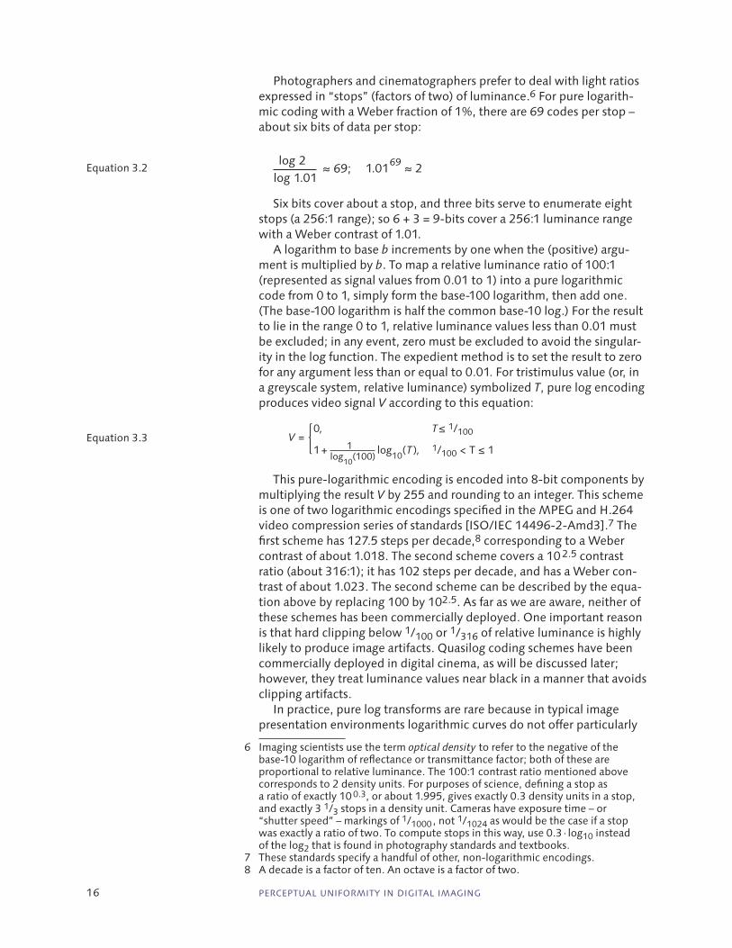
Photographers and cinematographers prefer to deal with light ratios expressed in “stops” (factors of two) of luminance.6 For pure logarith-mic coding with a Weber fraction of 1%, there are 69 codes per stop – about six bits of data per stop:
1.0169 ≈ 2 log 1.01log 2
≈ 69;Equation 3.2
Six bits cover about a stop, and three bits serve to enumerate eight stops (a 256:1 range); so 6 + 3 = 9-bits cover a 256:1 luminance range with a Weber contrast of 1.01.
A logarithm to base b increments by one when the (positive) argu-ment is multiplied by b. To map a relative luminance ratio of 100:1 (represented as signal values from 0.01 to 1) into a pure logarithmic code from 0 to 1, simply form the base-100 logarithm, then add one. (The base-100 logarithm is half the common base-10 log.) For the result to lie in the range 0 to 1, relative luminance values less than 0.01 must be excluded; in any event, zero must be excluded to avoid the singular-ity in the log function. The expedient method is to set the result to zero for any argument less than or equal to 0.01. For tristimulus value (or, in a greyscale system, relative luminance) symbolized T, pure log encoding produces video signal V according to this equation:
log10
(100)1
V = 1 + log10(T ), 1/100 < T ≤ 1
T≤ 1/1000,Equation 3.3
This pure-logarithmic encoding is encoded into 8-bit components by multiplying the result V by 255 and rounding to an integer. This scheme is one of two logarithmic encodings specified in the MPEG and H.264 video compression series of standards [ISO/IEC 14496-2-Amd3].7 The first scheme has 127.5 steps per decade,8 corresponding to a Weber contrast of about 1.018. The second scheme covers a 10 2.5 contrast ratio (about 316:1); it has 102 steps per decade, and has a Weber con-trast of about 1.023. The second scheme can be described by the equa-tion above by replacing 100 by 102.5. As far as we are aware, neither of these schemes has been commercially deployed. One important reason is that hard clipping below 1/100 or 1/316 of relative luminance is highly likely to produce image artifacts. Quasilog coding schemes have been commercially deployed in digital cinema, as will be discussed later; however, they treat luminance values near black in a manner that avoids clipping artifacts.
In practice, pure log transforms are rare because in typical image presentation environments logarithmic curves do not offer particularly
6 Imaging scientists use the term optical density to refer to the negative of the base-10 logarithm of reflectance or transmittance factor; both of these are proportional to relative luminance. The 100:1 contrast ratio mentioned above corresponds to 2 density units. For purposes of science, defining a stop as a ratio of exactly 10 0.3, or about 1.995, gives exactly 0.3 density units in a stop, and exactly 3 1/3 stops in a density unit. Cameras have exposure time – or “shutter speed” – markings of 1/1000 , not 1/1024 as would be the case if a stop was exactly a ratio of two. To compute stops in this way, use 0.3 · log10 instead of the log2 that is found in photography standards and textbooks.
7 These standards specify a handful of other, non-logarithmic encodings. 8 A decade is a factor of ten. An octave is a factor of two.

CHAPTER 3 PERCEPTUAL UNIFORMITY IN DIGITAL IMAGING 17
good approximation of the perceptual response to luminance. For a better approximation, we turn to the CIE’s definition of lightness.
Lightness
The Weber-Fechner Law was based upon the assumption that thresh-olds ( just noticeable differences, JNDs) can be meaningfully integrated. In the 1950s and 1960s, S. Smith Stevens criticized the Weber-Fechner law, declaring that “A power function, not a log function, describes the operating characteristic of a sensory system” [Stevens 1961]. Stevens’ objection was that since thresholds are defined by uncertainties, inte-grating them would be just accumulating uncertainties. Stevens devised and conducted psychophysical experiments based upon magnitude estimation to obtain more direct measures of the relationship between physical stimulus and perceptual response. He concluded that lightness could be approximated by the 0.33-power – that is, the cube root – of relative luminance. His results agreed quite well with investigations made decades earlier by Albert E. O. Munsell [1933], son of Albert H. Munsell [1915].
In the context of the historical Weber-Fechner logarithm and Stevens’ power function, an estimate of vision’s lightness response, symbolized L*, was eventually standardized by the CIE in 1976. The definition is essentially unchanged in today’s colour science stan-dards [CIE 15]. Given relative luminance, CIE L* returns a value between 0 and 100; a “delta” (difference, ΔL* ) of 1 is taken to approximate the threshold of vision for luminance differences. The L* function is basic-ally a power function with what we call an “advertised” exponent of 1/3 – that is, a cube root. A linear segment is inserted near black, below relative luminance of about 1%; the power function segment is scaled and offset to maintain function and tangent continuity at the break-point. See Figure 3.1.
Figure 3.1 CIE Lightness , denoted L*, estimates the perceptual response to light intensity (technically, relative luminance). Here L*, scaled to the range 0 … 1, is overlaid by power function having an exponent 0.42, the exponent that best fits L*. The L* function involves a cube root – that is, a 1/3-power function – but the power function incorporated into L* is scaled and offset. I also overlay a cube root onto the plot: A pure cube root is a poor approximation to L*.
00
20
40
60
80
100
0.2 0.4 0.6 0.8 1.0
Tristimulus value, T
Ligh
tnes
s, L
* (o
r es
tim
ate)
L*(T)
100·T0.42
100·T1/3

18 PERCEPTUAL UNIFORMITY IN DIGITAL IMAGING
The linear segment at relative luminance less than about 0.01 was introduced for mathematical convenience [Pauli 1976] and not for any visual reasons. What effect the linear segment has on perceptual uni-formity is an open question. The technical literature is rife with state-ments that L* is a cube root [McCann 1998, Richter 1980]. However, the scaling and offset cause the function to approximate an “effective” 0.42-power over its entire range.
Display characteristics and EOTF
In the era of the CRT (1941 – 2011), the electrostatic characteris-tics of the electron gun of the CRT imposed an EOTF that was well approximated by a power function from voltage input to light out-put. The symbol γ (gamma) represented the exponent at the dis-play. Although the CRT is gone, the EOTF remains: In a properly adjusted [ITU-R BT.1886] studio HD display, “gamma” is close to 2.4.
In computing, the sRGB standard [IEC 61966-2-1, Stokes 1996] establishes an EOTF that is effectively a pure 2.2-power function. (Veiling glare in the display’s ambient environment is expected to cause an additive increase in tristimuli.) The sRGB standard also includes an alternate EOTF that incorporates a linear segment.
In video and HD, gamma has historically been poorly standardized or not standardized at all. In 2011, after several decades of inaction, the ITU-R standardized the value 2.4 [ITU-R BT.1886], carefully chosen to codify current practice at the time (and for many years earlier). A 2.4 power is a very close match to the inverse of the L* function; see Figure 3.2.
Virtually all non-CRT image display equipment, including obsolete plasma display panel (PDP) direct view displays and today’s liquid crys-tal display (LCD), digital light processing (DLP) projectors, and liquid crystal on silicon (LCoS) projectors, are designed to mimic the histor-ical behaviour of CRTs. In displays such as DLP that involve physical
Figure 3.2 EOTF standardized in BT.1886 is a 2.4-power function from video signal (pixel value) to tristimulus. The gamma of a display system – for example, a studio HD display, or the reference sRGB EOTF – is the numerical value of the exponent of the power function. Here, the inverse of the CIE L* function is overlaid: It is evident that a 2.4-power function is a very close match to the inverse of L*. (A 3.0-power function is overlaid on the graph; clearly, a cube function is a rather poor match to the inverse of L*.)
0
0.2
0
0.4
0.6
0.8
1.0
0.2 0.4 0.6 0.8 1.0
Tr
isti
mul
us v
alue
, T
Video signal value, V
V3
L*(-1)(100·V )
V2.4

CHAPTER 3 PERCEPTUAL UNIFORMITY IN DIGITAL IMAGING 19
behaviour that converts signal to light in a linear manner, a nonlinear function (“degamma,” or “inverse gamma”) is provided by signal pro-cessing, typically incorporating one or more lookup tables (LUTs). In displays such as LCDs that involve nonlinear physical transducers, signal processing incorporates a function that imposes the difference between the desired 2.2- or 2.4-power-law behaviour of the image exchange standard and the inverse of the native characteristic of the transducer.
Eight‑bit pixel components
Eight-bit pixel components are very widely used in digital imaging. It is perceptually uniform coding, imposed by the nonlinear character-istics of standard displays, that makes 8-bit components practical for continuous-tone imaging. (Another factor making 8-bit components practical is that noise causes spatial diffusion of quantization error.)
If eight-bit components were used to encode linear-light values, with black at 0 and white at 255, a Weber contrast of 255/254 – about 1.004 – is obtained at white, code 255. As pixel value drops below code 100, the Weber contrast would increase above 1.01; the boundary between adjacent pixel values would be susceptible to being visible as “con-touring” or “banding.” At pixel value 20, the Weber contrast would be 1.05, high enough that visible artifacts would be likely.
Figure 3.3 plots L* as a function of code value for linear-light coding; for the 1.8-power coding typical of graphics arts (e.g., Macintosh prior to Mac OS X version 10.6); and for pure power functions having expo-nents of 2.2 (sRGB), 2.4 (studio video), and 2.6 (digital cinema, to be discussed). EOTF power function exponents of 2.2, 2.4, and 2.6 are all quite perceptually uniform, evidenced by their straight-line behaviour over most of the range of pixel values in Figure 3.3.
Figure 3.3 CIE Lightness (L*) value as a function of pixel value are plotted for several pure power function EOTFs, with exponents indicated. Linear-light coding (exponent 1.0) exhibits poor perceptual uniformity above L* 60, where the slope of the curve is diminished: one bit is wasted compared to the other codes. Linear-light coding also exhibits poor perceptual uniformity below L* of 40: The slope of the curve is high, and one additional bit would be necessary to achieve visual performance comparable to the other codes. The 1.8-power typical of graphics arts images exhibits good perceptual uniformity. Exponents of 2.2 (sRGB), 2.4 (studio video and HD) and 2.6 (digital cinema) all exhibit excellent perceptual uniformity; the higher the power, the better the performance in very dark tones (as evidenced by the hockey-stick shape close to black).
0.20 0.4 0.6 0.8 1.0
20
0
40
60
80
100
Pixel value, normalized
Ligh
tnes
s, L
*
2.22.4
2.6
1.8
1.0

20 PERCEPTUAL UNIFORMITY IN DIGITAL IMAGING
It is frequently claimed that 8-bit imaging has a “dynamic range” of 255:1 (or 256:1). To pick five of many examples in the literature:
An 8‑bit image has a dynamic range of around 8 stops. [Corke 2011]
Most of the images made for display on contemporary monitors have a dynamic range of only 256:1 per color channel, because that’s all that most monitors are built to support. [Mather 2007]
A typical JPEG, TIFF, BMP image has 8 bits per color or a maximum dynamic range of 256 per color channel (256:1). [Aliaga 2007]
A graphic image file with 8‑bits signal depth in each channel has a dynamic range of 255:1, corresponding to a maximum density of 2.4. [Kim 2006]
A range of 256 brightness steps is not adequate to cover a typical range from 0 to greater than 3 in optical density with useful pre‑cision, because at the dark end of the range, 1 part in 256 repre‑sents a very large step in optical density. [Russ 2006, p. 28]
Such claims arise from the implicit assumption that image data codes (pixel component values) are linearly related to light. For commer-cial imaging systems, that assumption is nearly always false: Eight-bit image data is almost universally coded nonlinearly, assuming a 2.2- or 2.4-power function (comparable to that of sRGB or BT.1886) at the display. Consequently, the dynamic range associated with code 1 is not 255:1 or 256:1, but about 200 000:1, as computed here:
200 0001
≈ 0.000 005 ≈ 2551 2.2( )Equation 3.4
In the fourth quoted statement above, 2.4 is the optical density corresponding to optical transmittance of 1/255 . In the fifth statement, optical density of 3.0 corresponds to 1000:1 contrast ratio, typical of very high quality displayed imagery. Covering a range of 3.0 in optical density with 8-bit coding using pure logarithmic pixel values yields 85 pixel values per decade (or 25.5 pixel values per stop), and a Weber contrast of 10 3/255, about 1.027. Contrary to the fourth author’s claim, quantizing a 3.0 density unit range into an 8-bit pixel value offers per-formance comparable to 8-bit coding of L*.
Another aspect of claims commonly found in the literature, implicit in all five quoted statements above, is that code 0 is disregarded – for no legitimate reason. In a simplistic, idealized system, you could take code 0 to produce luminance of zero, in which case the ratio of max-imum to minimum luminance – the dynamic range – is infinity! In practice, physical factors lead to minimum luminance greater than zero. The actual minimum luminance is an important aspect of the visual experience. If dynamic range is to characterize the visual experience, dynamic range must be defined as a ratio between physical quantities.9
9 As a thought experiment, consider linear-light 8-bit greyscale imaging with pixel values from 1 to 220 driving a display having black at 1 nt and white at ▶

CHAPTER 3 PERCEPTUAL UNIFORMITY IN DIGITAL IMAGING 21
When nonlinear coding is used, dynamic range is not a ratio of image data values.
Comparing 2.2‑ and 2.4‑power EOTF with CIE L*
As described earlier, ΔL* of unity is widely agreed to approximate the visual threshold between luminance levels. The ratio of luminance between L* values of 99 and 100 is about 1.025 – that is, the relative luminance difference at threshold is 2.5% (the Weber fraction):
0.975 ≈ L*(−1) (99)Equation 3.5
As relative luminance decreases, the luminance ratio between adjacent L* values increases, as shown in Figure 3.4. At L* of 8 (relative luminance just less than 0.01) the relative luminance ratio has reached 1.125, that is, a Weber fraction of 12.5%.10 The L* scale assigns 92 levels – or 93, including the endpoints – across a 100:1 range of relative luminance. Assuming that the visual threshold is 1 ΔL* unit, seven bits suffice to encode L* values.
Eight-bit digital studio video has 219 steps between black and white, and is standardized with a 2.4-power function at display [ITU-R BT.1886]; sRGB has 255 steps, and assumes a 2.2-power [IEC 61966-2-1]. These counts of possible integer pixel
▶ 220 nt. Contrast ratio, or dynamic range, is 220:1. Now, modify the graphics subsystem driving the display to add an offset of +15. The offset values appear in image files, and appear across the hardware interface to the display; pixel values now range 16 to 235. Modify the display signal processing to subtract 15 from the incoming data values. Has the dynamic range now dropped from 220:1 to 235/16, or about 15:1? Or is it unchanged?
10 Take the first derivative of the inverse of L* then divide by the inverse of L*; add one to get the Weber contrast.
Figure 3.4 Ratio of relative luminance values for unit ΔL*, across the L* range from 1 to 100. Starting at the right, between L* values 99 and 100, there is a 1.025 ratio (2.5%) between relative luminance values at the assumed threshold of unity ΔL*. As L* decreases, the “delta” increases. At L* of 8 – corresponding to relative luminance of about 1%, or contrast ratio of about 100:1 – the ratio has increased to 1.125. As relative luminance decreases, image coding can use fewer and fewer pixel values per stop without the differences being visible.
208
0 40 60 80 1000.01
0.50
0.20
0.10
0.05
0.02C
on
tras
t, ∆
Y /Y
(log
scal
e)
Lightness, L*

22 PERCEPTUAL UNIFORMITY IN DIGITAL IMAGING
values are intermediate between the 462 codes of pure log coding at a Weber contrast of 1.01 and the 92 codes of direct L* coding. In Photoshop LAB coding [Adobe 2002], and in the LAB PCS of the ICC standard [ISO 15076], L* values are scaled by 2.55 for encoding into the range 0 through 255: The coding has about 2.5 digital code values per L* unit – that is, a Weber fraction of about 1% at white.
We have discussed the number of codes across 100:1 contrast ratio, or two decades of luminance. A particular imaging application may require a range less than or greater than 100:1. Also, typical photo-graphic images have a certain amount of noise; visibility of contouring will be reduced by noise, and quantization will be less demanding.
A discussion of perceptually uniform decoding and display in the domain of medical imaging is found in Chapter Chapter 7, Analysis of greyscale medical image display, on page 81.
Picture rendering II
All imaging applications involve non-ideal displays, and almost all applications involve image viewing in conditions different from those in effect at the time of image capture. The goal of most imaging applications is not to match relative luminance values between the scene and the display, but instead, to match the ultimate viewers’ expectation of the appearance of the scene. Engineers and scientists unfamiliar with colour science are usually surprised to learn that the intended appearance is not achieved by matching relative luminance values between scene and display: Preserving appearance almost always requires manipulating the tristimulus value estimates between the scene and display. Manipulation is typically accomplished either algorithmically (for example, by firmware in a digital still camera) or manually, by a skilled specialist (such as a photographer or a colourist) [Fairchild 2005, Giorgianni 2008, Hunt 2004, ISO 22028-1].
In many commercial imaging systems, including video and digital still photography, baseline picture rendering is achieved by using an OETF that roughly approximates a 0.5-power function (which is the pure power function that best fits BT.709), rather than the 0.42-power that would perfectly invert a 2.4-power EOTF at display. The combination of an effective 0.5-power OETF (e.g., that of BT.709) and a 2.4-power EOTF (e.g., that of BT.709) imposes an end-to-end 1.2-power. For image data acquired at 3200 nt in an average surround, a 2.4-power function is a first approximation for rendering onto a display having reference white at about 100 nt viewed in a very dim surround.
If an imaging application is required to maintain relative luminance values from an encoder to a decoder, then the OETF (at encoding) should be chosen as the mathematical inverse of the EOTF that will be imposed at decoding and display. For the near-ideal 2.4 power used in studio video display, you would expect the encoder to have as its expo-nent the reciprocal of 2.4 – that is, about 0.42. Such cases are rare.
Gamma correction
In nearly all commercial imaging systems, an OETF – or loosely, “gamma correction” – is imposed at encoding, often immediately following transduction in the sensor. Gamma correction takes estimated R, G, and B (radiometrically linear) tristimulus estimates from the scene, and

CHAPTER 3 PERCEPTUAL UNIFORMITY IN DIGITAL IMAGING 23
forms (nonlinear) R’, G’, and B’ quantities to represent those tristimu-lus values in a smaller number of bits. The primes signify the nonlinear relationship to light power. To achieve perceptual uniformity, the OETF roughly approximates vision’s lightness sensitivity by imposing a function comparable to L*. Decoding and display of digital image data involves an EOTF that approximates the inverse of lightness sensitivity for each of the R, G, and B components.
In a historical CRT display, the electrostatic characteristics of the electron gun caused the CRT to impose an EOTF that was approximately a 2.4-power function from voltage input to light output. The symbol γ (gamma) represents the exponent at the display: A studio reference display is said to have gamma of about 2.4. Historically, gamma in video and HD was poorly standardized or not standardized at all. In 2011, when CRTs were rapidly falling into disuse, the ITU-R standardized the value 2.4 [ITU-R BT.1886]. Although CRT displays are now obsolete, the image coding standardized in BT.1886 stands: It remains completely viable and economically important.
To achieve perceptual uniformity, the OETF roughly approximates vision’s lightness sensitivity by imposing a function comparable to L*. Decoding and display of digital image data involve an EOTF that approximates the inverse of lightness sensitivity for each of the R, G, and B components.
Gamma correction is often described as a pair of inverse functions; for example, see Figure 3.5, taken from Rowlands [2017]. However, using an OETF at the camera that is the inverse of the display’s EOTF fails to incorporate any picture rendering. If the captured scene has light levels comparable to the ultimate display – say, diffuse white in the scene has luminance of 80 cd · m−2 – the resulting imagery may be visually correct. However, typical acquisition takes place in environ-ments where a diffuse white reflector exhibits absolute luminance much higher than 80 cd · m−2, and failure to impose picture rendering is highly likely to produce displayed images that are judged as unsatisfactory.
Figure 3.5 Gamma function as presented by Rowlands [2017, p 2-9] shows a 2.2-power function, standardized for the EOTF of an sRGB display. The graph also shows the mathematical inverse, approximately a 0.45-power function, and the identity function. Rowlands’ text explains that “gamma correction” should mathematically invert the display’s EOTF. However, when used with a 2.2-power EOTF, a 0.45-power OETF would not apply any picture rendering.

24 PERCEPTUAL UNIFORMITY IN DIGITAL IMAGING
Tristimulus values
As mentioned earlier, a suitably-weighted sum of tristimuli yields lumin-ance [SMPTE RP 177], and that luminance can be augmented with two other linear-light components (having prescribed spectral composition) to yield tristimuli.
In practice, cameras typically depart from the spectral sensitivities prescribed by CIE standards, consequently, tristimulus values and luminance with respect to the scene are usually estimated, not exact: Image data incorporates the effect of the imperfect match to the CIE Standard Observer (that is, camera metamerism). However, the usual goal of digital imaging is to produce the intended presentation on the ultimate display device. Image data is typically referenced to a set of additive primaries. (The sRGB standard applies to general computing, and the BT.1886 standard applies to HD; not coincidentally, these stan-dards share the same set of primaries.) Faithful display is achieved on a display device that conforms to the intended colorimetric standard. Once sensed and recorded, image data is associated with the colour representation defined in the interchange standard. In professional imaging, and in content creation, tristimulus values and luminance are then exact with respect to a reference additive RGB display (for example, a studio display). Content creators expect that tristimuli and luminance are reasonably well approximated at the ultimate consumer displays.
Modern misconceptions
The 525-line monochrome (greyscale) television system was designed in the 1940s; its extension to colour was designed in the late 1940s and early 1950s. Publications of the time [Hazeltine 1956, Kallmann 1940, Maloff 1939, Mertz 1950, Oliver 1950} make clear that the design-ers of those systems understood the importance of nonlinear coding to achieve good visual performance (although they did not give the concept the name perceptual uniformity).
Astonishingly, since about 1960, the significance of perceptual uniformity has been largely forgotten! Engineers are always desirous of linearity; video engineers apparently came to believe that the purpose of gamma correction was to overcome a supposed deficiency – that is, nonlinearity of the CRT. They realized that the sensible place to perform the “correction” was close to the transmitter, so as to avoid millions of nonlinear circuits in receivers. The link to perceptual uniformity was apparently forgotten. Widespread misunderstanding among television engineers of the fundamental reason for “gamma correction” remains rampant even today. As I stated [2003, p. 258]:
If gamma correction were not already necessary for physical reasons at the CRT, we would have to invent it for perceptual reasons.
You can test your colleagues: Ask, “If television displays in 1953 had exhibited a linear relationship between voltage applied to the CRT and light output, would television standards have included gamma cor-rection?” Anyone who answers “Of course not!” does not appreciate the importance of perceptual uniformity. It is clear from their writ-ings that the inventors of analog television coding [Hazeltine 1956,
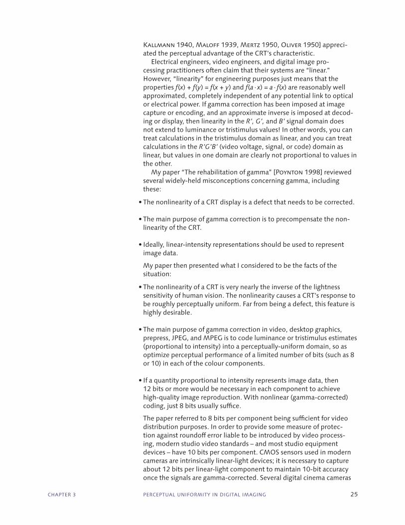
CHAPTER 3 PERCEPTUAL UNIFORMITY IN DIGITAL IMAGING 25
Kallmann 1940, Maloff 1939, Mertz 1950, Oliver 1950] appreci-ated the perceptual advantage of the CRT’s characteristic.
Electrical engineers, video engineers, and digital image pro-cessing practitioners often claim that their systems are “linear.” However, “linearity” for engineering purposes just means that the properties f(x) + f(y) = f(x + y) and f(a · x) = a · f(x) are reasonably well approximated, completely independent of any potential link to optical or electrical power. If gamma correction has been imposed at image capture or encoding, and an approximate inverse is imposed at decod-ing or display, then linearity in the R’, G’, and B’ signal domain does not extend to luminance or tristimulus values! In other words, you can treat calculations in the tristimulus domain as linear, and you can treat calculations in the R’G’B’ (video voltage, signal, or code) domain as linear, but values in one domain are clearly not proportional to values in the other.
My paper “The rehabilitation of gamma” [Poynton 1998] reviewed several widely-held misconceptions concerning gamma, including these:
• The nonlinearity of a CRT display is a defect that needs to be corrected.
• The main purpose of gamma correction is to precompensate the non-linearity of the CRT.
• Ideally, linear-intensity representations should be used to represent image data.
My paper then presented what I considered to be the facts of the situation:
• The nonlinearity of a CRT is very nearly the inverse of the lightness sensitivity of human vision. The nonlinearity causes a CRT’s response to be roughly perceptually uniform. Far from being a defect, this feature is highly desirable.
• The main purpose of gamma correction in video, desktop graphics, prepress, JPEG, and MPEG is to code luminance or tristimulus estimates (proportional to intensity) into a perceptually-uniform domain, so as optimize perceptual performance of a limited number of bits (such as 8 or 10) in each of the colour components.
• If a quantity proportional to intensity represents image data, then 12 bits or more would be necessary in each component to achieve high-quality image reproduction. With nonlinear (gamma-corrected) coding, just 8 bits usually suffice.
The paper referred to 8 bits per component being sufficient for video distribution purposes. In order to provide some measure of protec-tion against roundoff error liable to be introduced by video process-ing, modern studio video standards – and most studio equipment devices – have 10 bits per component. CMOS sensors used in modern cameras are intrinsically linear-light devices; it is necessary to capture about 12 bits per linear-light component to maintain 10-bit accuracy once the signals are gamma-corrected. Several digital cinema cameras

26 PERCEPTUAL UNIFORMITY IN DIGITAL IMAGING
offer 14-bit linear-light analog-to-digital converters, and thereby offer about 12 bits of quantization performance when coded perceptually.11 Roughly speaking, representing colour components in a perceptually uniform manner saves 2, 3, or 4 bits per component compared to rep-resentation in linear-light form.
Modern practice in video and HD
Today’s HD studio reference displays have gamma very close to 2.4. Reference white luminance of 100 cd · m−2 is standardized [SMPTE ST 2080-1]. Contrast ratio is typically about 3200:1. At program mastering, studio reference displays are viewed with a very dim sur-round, illuminated such that the surround luminance is about 1% of the reference white luminance.
Creative approval of program material in the studio environment causes not only the studio EOTF but also the studio viewing conditions to be implicit in the definition of the R’G’B’ exchange standard: It is implicit that the intended picture appearance at the consumers’ prem-ises is obtained from a comparable EOTF in a comparable environment. Should a consumer’s display characteristics or viewing condition differ substantially from the studio – for example, if the consumer display is brighter, or has inferior contrast ratio, or is located in a lighter surround than the studio – then image data should be altered at the consumer’s premises to yield a closer match to the intended appearance.
CRTs are now obsolete, and several display technologies have replaced them. None of the new display technologies – LCD, DLP, LCoS, or OLED/AMOLED – involves a native physical 2.4-power law like that of a CRT. Some people argue that emergent display technology gives us a chance to adopt linear-light encoding for video [Li 2005]. However, perceptual uniformity remains important for these reasons:
• Perceptually uniform coding maximizes the perceptual utility of a lim-ited number of bits – usually 8, or 10, or 12 – per component;
• Nearly all commercially important digital image storage and exchange standards call for perceptual uniformity; and
• Billions of stored images incorporate perceptual uniformity.
Modern practice in digital cinema
Standards for d-cinema mastering [SMPTE ST 431-1, SMPTE RP 431-2] call for R’G’B’ or X’Y’Z’ components (at the reference projector inter-face, or the digital cinema distribution interface, respectively) to be raised to the power 2.6 for display. The 2.6-power is imposed to invert perceptually uniform encoding. Compared to the 2.4-power EOTF of studio video, the 2.6-power offers improved visual performance in the low luminance and dark surround situation of the cinema.
DCI/SMPTE d-cinema standards are completely mastering-display- referred with respect to the standard 2.6-power EOTF. D-cinema
11 That 12-bit perceptual components suffice is demonstrated by the XYZ 1/2.6 EOTF −1 specified in SMPTE/DCI standards for digital cinema [SMPTE ST 431- 1]; however, a pure power function such as this is unsuitable as an OETF.

CHAPTER 3 PERCEPTUAL UNIFORMITY IN DIGITAL IMAGING 27
standards make no reference to a camera, and make no reference to post-production (apart from mastering).
There are no SMPTE/DCI standards for digital cinema acquisition; many techniques are in use. The basic principles outlined above apply when the cinematographer decides, based upon the scene being captured, upon a diffuse white reference near the top end of the digital coding scale. If specular highlights beyond diffuse white are to be accommodated, then the cinematographer may impose what an engineer might call a distortion of the code scale above diffuse white. The cinematographer may have reason to acquire a scene while deferring any decision about reference white – that is, the decision may be deferred until post-production. In that case it may be appro-priate to use an acquisition standard having a pure logarithmic code or a quasilog code with an appropriate number of digital code values per stop of scene-space luminance (“exposure”). For an example of a quasilog encoding commonly used in such situations (“FilmStream”) [SMPTE RDD-2].
In classic photochemical film historically used in cinema, a rough approximation to picture rendering is evidenced by the standard lab‑oratory aim density (LAD) practice [Pytlak 1976] that was ubiquitous in motion picture film laboratories, and is mimicked in digital cinema production: Relative luminance of about 0.18 in the scene produces optical density of about 1.06 in the print, and thereby produces relative luminance on-screen of 10 −1.06, or about 0.087. Approximating the end-to-end function as a pure power function, the resulting effective end-to-end power function exponent is found to be about 1.4:
0.18g = 10−1.06 ≈ 0.087; g = −1.06log 0.18
≈ 1.4Equation 3.6
An 18% grey card is presented at 8.7% on-screen. As a second point of reference, camera negative film stock has
a film gamma of roughly 0.6, and print film stock has a film gamma of roughly 2.5. The product of 0.6 and 2.5 – that is, 1.5 – is an approxima-tion of the exponent of the effective end-to-end power.
The end-to-end exponent of 1.4 or 1.5 for cinema is larger than the 1.2 of HD because the cinema display is darker (having a reference white of 48 nt compared to 100 nt of HD), and because the surround is black (0% in cinema) as opposed to dim (about 1%) in HD mastering.
This chapter mainly concerns quantization of each colour component into a fairly small number of bits – say 8 or 10. Where that constraint is lifted, for example where 16 bits are available per component, then per-ceptual uniformity is still useful, but the ratios of luminance or tristimu-lus values between codes are lower than the visual threshold (even if components are coded in radiometrically linear, “linear-light” manner). In digital cinema acquisition and processing, OpenEXR [Kainz 2004] coding is widely used. That coding uses 16 bits per component. Code values are represented in binary floating point, with one sign bit, five base-2 exponent bits, and ten fraction bits. The floating point encoding imposes a fixed Weber contrast (of about 0.1%) over nearly the entire range of coded values. The logarithmic coding imposes a high degree of perceptual uniformity across a dynamic range of up to 2 30.
28 PERCEPTUAL UNIFORMITY IN DIGITAL IMAGING
Perceptual quantization (PQ)
Peter Barten [1999, 2004] developed an analytical model of the lumin-ance threshold of human vision over a wide range of luminance levels. The model is parameterized by eight or so parameters.
The medical imaging community adapted Barten’s model to grey-scale medical imaging, through suitable choice of the model’s param-eter values. The standards group for Digital Imaging Communications in Medicine (dicom) standardized the grayscale display function (GSDF) [ACR/NEMA 2009]. A detailed discussion is found in Chapter 7, Analysis of greyscale medical image display, on page 81.
In an unrelated effort, Dolby Labs adapted Barten’s model to high dynamic range (HDR) video; conducted experiments to establish suitable parameter values; and developed a perceptual quantizer (PQ) [Miller 2013]. SMPTE standardized the scheme [ST 2084]. The stan-dard is explicitly mastering-display-referred; its EOTF maps a 10-bit perceptually coded video signal12 into absolute luminance values between nominal 0 and 10 000 nt. The PQ comprises an EOTF and its inverse (an EOTF−1). Perceptual quantization takes radiometric values and produces integer code values at luminance/tristimulus values at perceptual increments: the quantizer operates at the encoding stage. Stated succinctly, PQ is an EOTF−1. However, in common language PQ has come to denote the EOTF, what would more accurately be called the dequantizer.
Summary
Perceptual uniformity is a tremendously important aspect of digital image coding, particularly in video, HD, digital cinema, medical imaging, digital still photography, and desktop computer graphics. Without it, 10, 11, or 12 bits per component would be necessary, instead of the 8 bits common in consumer equipment or the 10 bits common in professional video and HD. If L* is taken as a model for perceptual uniformity, 2.2- or 2.4-gamma is a remarkably good match. Perceptual uniformity was appreciated half a century ago, yet is either poorly understood or not recognized at all by a surprisingly large num-ber of image scientists and engineers working today.
12 The standard 10-bit digital video HD-SDI interface has codes between 64 and 940 (inclusive). HDR seeks to extend the luminance/tristimulus range covered, compared to HD. Paradoxically, though, in HDR, use of the footroom and headroom codes is prohibited.

29
4 Lightness mappings for image coding
Visual sensitivity and perception of lightness are nonlinear functions of light power. In most applications of digital imaging, we seek a percep-tually efficient coding of luminance – that is, a coding where increasing the coded value by a certain arithmetic increment produces roughly the same increase in (perceived) lightness across the whole tone scale. In the fixed-point integer coding that is nearly ubiquitous in commercial digital imaging, that increment will typically be one code level; eight-bit coding offers 256 distinct levels. Such an approach is the basis for the sRGB coding in desktop computing, the BT.1886 coding used in digital video and HD, the DICOM standard in digital medical imaging, stan-dard digital cinema encoding, and other applications. There is a big gap between the theory of sensation and its application to image system design. This chapter seeks to narrow that gap.
We outline CIE lightness (L*), and review the historical development of models of lightness perception including the models (“laws”) of Weber, Fechner, de Vries, Rose, Stevens, and Barten. We then sur-vey practical image coding systems used in digital still photography, desktop computing, digital video and HD, digital cinema, and medical imaging, to see how they are related to the theoretical models.
Absolute and relative luminance (L and Y )
We’re concerned with greyscale, luminance, and related quantities. The naïve extension to colour is to apply the same lightness function to each of three tristimulus components. Such is the case in many colour imaging systems like sRGB [ISO 61966], where identical per-ceptually relevant electro‑optical transfer functions (EOTFs) are applied to each component. At least one widely used standard, BT.1886 [ITU-R BT.1886] defines the EOTF using the term luminance for each component individually; implicitly, the definition applies when the other two components are zero.
The terminology, symbols, and units of light are complex and confus-ing [Halsted 1993, Palmer 1993]. We’ll review.
In radiometry, L symbolizes radiance; it has SI units of W · sr −1 · m −2. When spectral radiance is weighted by the CIE luminous efficiency function, the result is absolute luminance, symbolized Lv , having units of cd · m −2. When radiometry is absent from the context, colour scien-tists drop the v subscript, as we will do in what follows. Radiance and luminance are highly useful quantities because they are invariant in

30 LIGHTNESS MAPPINGS FOR IMAGE CODING
transport through lossless media (such as air): you can measure radiance or luminance at the source of light, at a sensor, or anywhere in between.
When absolute luminance is normalized with respect to a reference, the result is relative luminance (Y), a dimensionless quantity. The nor-malization amounts to a crude approximation of the lightness constancy of the human visual system; normalization typically takes a form such as this:
Y = LLW
or Y = L5 LM
Equation 4.1
The first option divides luminance by LW (symbolizing the absolute luminance of a perfect or near-perfect white diffuse reflector in the scene under the prevailing illuminant). In the second option, LM sym-bolizes the absolute luminance of middle grey; normalization assumes an “average surround” of 18% or 20%, and adopts a reference white of 5 times that luminance.
Historically, colour scientists expressed relative luminance Y with respect to a reference of 100; that is, the Y value was a percentage. Nowadays, a reference value of 1 is common; that is, the reference range of Y is from 0 (reference black) to 1 (reference white).
In colour science, relative luminance Y is one of three distinguished tristimulus values; the other two incorporate colour aspects of the stimulus and are denoted X and Z. I say “distinguished” because XYZ are standardized by the famous CIE standard that originated in 1931. XYZ form the bases for other sets of tristimulus values (such as various forms of LMS and various forms of RGB). Robert Hunt and Michael Brill agree that tristimulus values properly have no units [Hunt 1997].1
Brightness and lightness
Brightness is defined by CIE 17.4 [CIE 1987; see also Fairchild 2005] as the attribute of a visual sensation according to which an area appears to emit more or less light. This definition is subjective: Brightness properly has no objective metric. Brightness has no top end; it is not relative to anything. Brightness is most succinctly described as apparent amount of light (or apparent luminance.)2
Lightness is defined by the CIE as the brightness of an area judged relative to the brightness of a similarly illuminated area that appears to be white or highly transmitting. Lightness is by definition relative to a reference. Lightness generally describes diffusely reflecting surfaces; lightness is most succinctly described as apparent reflectance.3
Strictly speaking, the CIE’s definition of lightness is subjective (like that for brightness). Brightness is what Engeldrum [2000, 2004] calls a “-ness” word: it describes a perceptual attribute. Nevertheless, in 1976 the CIE defined an objective quantity that is the perceptual
1 Some spectroradiometers report absolute luminance and X and Z tristimuli relative to that value. Absolute luminance is typically mislabelled Y. The other two quantities – though not tristimuli – are commonly labelled X and Z.
2 From the 1930s through the 1960s, the term brightness and the symbol B were used to refer to what today we would call luminance. The term brightness remains in use today in the physical sense in certain fields such as astronomy.
3 Illumination is necessary to measured or perceive reflectance. There is spectral interaction of illumination and object reflectance. Here we assume wideband illumination. ̀

CHAPTER 4 LIGHTNESS MAPPINGS FOR IMAGE CODING 31
correlate of relative luminance. CIE lightness (L*) is a scaled and offset cube root of relative luminance, with a linear segment inserted below argument values of a percent or so. The range of L* is ordinarily from 0 to 100. L* values are intended to describe diffusely reflecting surfaces. Because lightness is computed from relative luminance, it incorporates visual lightness constancy.
Many authors describe CIE lightness as a cube-root function, but that description neglects the scaling and offset terms, which are sig-nificant to the nature of the function. The best pure power function fit to L* is obtained with an exponent of 0.42, not 0.333 (see Lightness on page 17 of Chapter 3).
The CIE L* calculation takes Y as its argument. The non-expert may interpret the division by Yn as dividing the argument Y by a reference absolute luminance to obtain relative luminance. In fact the CIE arith-metic for L* is doubly-normalized: Absolute luminance has already been normalized to form Y as in Equation 4.1. The division of Y by Yn in the definition of L* merely accommodates different conventions for the scaling of reference white.
L* is intended to describe diffusely reflective surfaces. L* is normal-ized to “white,” but CIE standards aren’t explicit about exactly what constitutes “white.” In hard-copy graphics arts, maximum luminance corresponds to the reflectance of the media (“paper white”); adaptation is nearly always determined by the viewing environment. For electronic displays the situation is more complex, as we will describe.
Contrast
Contrast refers to a measured or visual distinction between grey shades,4 ordinarily quantified by a large or small luminance ratio.
Contrast ratio is the ratio between a high luminance (often refer-ence white, perhaps the luminance of a perfect diffuse reflector or its representation on a display, or the maximum luminance attainable on a display) and a very low luminance (such as the minimum luminance that can be produced by a display in a given ambient environment).
A luminance increment, which we symbolize ΔL, is a small test lumin-ance added to a reference luminance L. When a pair of adjacent patches having luminance values L and L + ΔL are on the threshold of being distinguished by vision as different, ΔL is the threshold luminance incre‑ment. The relative threshold luminance increment – or more succinctly, contrast (C) – is the ratio ΔL/L. When adaptation effects are to be stud-ied, the test stimulus is viewed against a background having luminance symbolized here as L0 .
Weber contrast (here symbolized W ) is the contrast at the threshold of perceptibility. At high absolute luminance levels – say outdoors at noon on a clear day, when a white card reflects perhaps 10 000 nt – normal vision has a threshold luminance increment of about 100 nt, a contrast threshold of about 0.01 (i.e., one percent) and contrast sensitivity of 100.
In describing visual contrast, many authors use the term intensity (symbolized I ) and plot Δ I values (or Δ I/I fractions) on threshold versus intensity (TVI) plots. The term intensity is loaded: We must digress. Intensity of sound has dimensions of power per unit area. Sound inten-
4 More generally, contrast involves colour distinctions.

32 LIGHTNESS MAPPINGS FOR IMAGE CODING
sity is different at different distances from a source; sound follows the inverse square law; and sound intensity is directly correlated to auditory perception.5 Intensity of light, however, is conceptually very different: Luminous flux is comparable to power, but luminous inten-sity has dimensions of flux per unit solid angle (not per meter squared). Light intensity is independent of distance from a source; ittensity is not characterized by the inverse square law.6 Luminous intensity may not be well understood, but it’s important: It’s one of just seven basic SI units.7 The SI unit for luminous intensity is the candela [cd], equivalent to a lumen per steradian.
To properly represent a visual stimulus, the dimensions of light incident on the retina properly include a per unit area term. The cor-rect quantity is luminance, and the proper SI unit is candela per meter squared [cd · m −2]. The prevalence of the term intensity in psychophys-ics seems to be due to psychophysicists studying many modalities of sensation, including studying the loudness of sound, and conflating the terms. The term intensity is common in computer graphics (for example, pixel intensity), but only in contexts where light is not being measured.
Historically, visual contrast results were presented in threshold versus radiance (TVR) plots [Wyszecki 1982]. No spectral assumptions are implicit in the term radiance (unlike luminance). Threshold versus lumin-ance would be more accurate, implying the standard CIE luminous efficiency spectral weighting.
Contrast sensitivity
Contrast sensitivity is the reciprocal of contrast at the visual threshold. The threshold is affected by the spatial extent (area) of the stimulus,
ordinarily expressed in degrees of visual angle. For spatially periodic stimuli (such as gratings), rather than characterizing the visual angle of one element of the stimulus, it is usual to characterize its spatial fre-quency in units of cycles per degree of visual angle (CPD).
The threshold is also affected by the temporal duration of the stimulus. The duration of a single flash can be expressed in seconds or milliseconds. For temporally periodic stimuli such as a rapidly flashing stimulus, rather than characterizing the duration of one flash, it is usual to characterize the temporal frequency in hertz [Hz].
Finally, the threshold is affected by the luminance to which the observer is adapted. Adaptation is affected by the ambient environ-ment, and affected by the scene or image being viewed. In viewing hard-copy material, adaptation is dominated by the ambient illumin-ance; the image itself contributes little. In cinema, the ambient environ-ment is almost completely dark; adaptation is controlled by the average luminance of the displayed imagery. In viewing a computer display, and in viewing television, adaptation is determined by a combination of the ambient environment and the displayed imagery.
5 Sound intensity is not to be confused with sound pressure level (SPL), which is typically measured in units of pascal [Pa], equivalent to newton per square meter [N · m−2]. SPL in decibels [dBspl] is 20 times the base-10 logarithm of a ratio of such quantities. SPL does not follow the inverse square law.
6 If a light source subtends an infinitesimal angle – if it’s a distant star, for example – then characterizing in terms of intensity is not appropriate.
7 The other six are length [m], mass [kg], time [s], electrical current [A], thermo-dynamic temperature [K], and amount of substance [mol].

CHAPTER 4 LIGHTNESS MAPPINGS FOR IMAGE CODING 33
Contrast sensitivity is the key psychovisual parameter that should allow us to explore the nature of the mapping from luminance to light-ness. However, the psychovisual literature dwells only briefly on con-trast sensitivity of what an engineer would call the zero frequency or DC term: the dependence of contrast sensitivity upon spatial and temporal frequency receives much more attention in the psychophysics literature than the DC case, so much so that the term contrast sensitivity function (CSF) has come to denote the spatial and temporal functions, but not the zero-frequency function.
Historical survey of lightness mappings
Mappings that estimate (perceptual) lightness from (physical) lumin-ance have been studied in many psychovisual experiments, with a diversity of results. Norwich [2003] states that “Hundreds, if not thou-sands, of pages have been published in this endeavor.” That statement falls on page 100 of Norwich’s 209-page work, so “hundreds” must be an underestimate. My guess is tens of thousands.
Since lightness is a sensation, the mapping can never be known precisely. However, there are several reasons why it is useful to have an approximation: to estimate the perceptibility of lightness differences; to form the basis for a perceptually uniform colour space; and to imple-ment perceptually uniform image coding.
Analytical estimations of the mapping fall into three main theoretical traditions, all of which are sufficiently well-established in the psycho-physics community to have become known as “laws” (albeit, empirical laws): Weber-Fechner, de Vries-Rose, and Stevens.
Weber‑Fechner
The Weber-Fechner approach, described in virtually all psychology textbooks, posits sensation as proportional to the logarithm of physical stimulus. Perceptible lightness increments (just‑noticeable differences, jnds) are taken to occur at constant ratios of luminance. Different researchers and different experiments establish contrast in the limit at between about 0.04 and 0.005 – that is, researchers estimate Weber contrast between about 4 percent and 0.4 percent.
The graph of Hecht [1924] is reproduced here as Figure 4.1. A Weber fraction of 1 or 2 percent is evident in the upper realms, above x-coordinate8 of about −0.50, that is, above about 1 nt. It is evident from Hecht’s graph that Weber’s Law fails at luminance levels below about 0.1 nt; indeed, Hecht claimed that the Weber-Fechner principle fails as a general principle. A few decades later, Hunt [1953] reiterated the failure of the Weber-Fechner “law.”
Weber’s conclusions were drawn from visual experiments equivalent to using what I call a half-moon stimulus, sketched in Figure 4.2: Weber asked when a human observer judged a patch having luminance L0+ΔL as perceptibly different from a patch having luminance L0 , the lumin-ance of the background. That experiment yields visual thresholds at the adaptation level. For purposes of this chapter, the half-moon subtends about 2˚ of the observer’s visual field.
8 Hecht’s x-axis reflects luminance in archaic units of millilambert [mL]. One mil-lilambert is about 3.426 nt.

34 LIGHTNESS MAPPINGS FOR IMAGE CODING
The crispening effect [Takasaki 1966] is familiar to colour appear-ance researchers: Vision is most sensitive to luminance difference when adapted to a luminance similar to the patches being compared. To examine thresholds at different adaptation states, a bipartite field such as that shown in Figure 4.3 can be used. The observer compares L and L+ΔL; for reasonably small patches (say, less than 2˚), the observer’s adaptation state can be set by changing the background luminance L0 . We’ll return to this stimulus in a moment.
0.00
01
0.00
1
0.01 0.1 1 10 100
1000
10 0
00 nt
Figure 4.1 Hecht’s 1924 graph with “intensity” in millilamberts, is augmented with a modern x-axis in cd · m −2 [nt]. Above −1.5 on the x-axis, corresponding to an absolute luminance of 0.1 nt, Weber’s Law behaviour occurs: The perceptual threshold occurs at a near-constant luminance ratio. Weber’s Law behaviour is maintained over several decades, until luminance above about 1000 nt, when a saturation mechanism takes hold. Below luminance of about 0.1 nt, visual contrast thresholds are consistent with the explanations of de Vries and Rose.
L+ΔL
L = L0
L L+ΔL
L0
Figure 4.2 “Halfmoon” stimulus symbolizes Weber’s stimulus. A just‑noticeable difference (JND) is typically observed when ΔL exceeds about 1% or 2% of L.
Figure 4.3 Bipartite field allows determining the contrast threshold at luminance L different from the adaptation luminance L0 .

CHAPTER 4 LIGHTNESS MAPPINGS FOR IMAGE CODING 35
De Vries and Rose
The Dutch physicist Hessel de Vries, one of the fathers of carbon dating, and Albert Rose, the inventor of the vidicon camera tube, independ-ently studied the properties of vision in light-limited situations [de Vries 1943, Rose 1948]. As absolute luminance decreases, the sta-tistical properties associated with detection of discrete photons cause greater and greater uncertainty. De Vries and Rose concluded that this “photon noise” causes uncertainty proportional to the square root of luminance. (Photon noise is sometimes called shot noise.) At luminance lower than about 0.1 nt, no useful visual information is to be gained by visual performance exceeding this threshold.
Schreiber [1991, Fig. 3.4] redrew Hecht’s graph (shown here in Fig-ure 4.4). He added two lines at low luminance. One has the −0.5 slope of the de Vries-Rose relationship; the other has slope −0.42, fitting Hecht’s data at low luminance. Schreiber’s redrawn graph suggests that the de Vries-Rose “law” explains the visual threshold at low lumin-ances, and that the Weber-Fechner “law” explains thresholds at high luminances. The transition occurs between absolute luminance values of 0.1 to 1 nt.
Schreiber discussed the effect of adaptation. Figure 4.5 reproduces his graph [1991, Fig. 3.8] illustrating that discussion. He shows four hypothetical contrast sensitivity curves, at adapting luminances L1 , L2 , L3 , and L4 . Each curve has a “U” shape showing that the maximum contrast sensitivity is achieved at the adapting luminance. Schreiber’s L0 represents the adaptation (or background) luminance in Figure 4.3. Schreiber argued that the contrast sensitivity of vision is highest at the adaptation luminance, represented by the “troughs” in Figure 4.5, where L and L + ΔL are both similar to L0 . Reducing L below the
0.00
01
0.00
1
0.01 0.1 1 10 100
1000
10 0
00 nt
0
Figure 4.4 Schreiber redrew Hecht’s graph , transforming Hecht’s Δ I/I data to a log scale on the y-axis and adding a dashed line in the left half of the graph to indicate the de Vries-Rose slope of −0.5. Schreiber’s graph has been augmented here with modern units of cd · m −2 [nt]. Schreiber placed an arrow at about 100 nt; his arrow identifies the minimum Weber fraction, about 10 −1.7 or 0.02, that is, 2 percent.

36 LIGHTNESS MAPPINGS FOR IMAGE CODING
adaptation luminance causes the contrast sensitivity to diminish – the left-hand leg of the U-figures in Figure 4.5. Increasing L above the adaptation luminance also causes the contrast sensitivity to diminish – the right-hand leg of the U-figures. Schreiber deleted the numerical scales from this graph: Apparently he didn’t want readers to make quantitative conclusions from it.
Samei is concerned with medical imaging. The graph in Figure 4.6 is reproduced from his work [Samei 2005, Fig. 4]; it shows a quanti-tative model of the adaptation phenomenon postulated by Schreiber. The “Barten model” indicated in his graph was adopted in the dicom GSDF function now widely used in medical imaging. The dicom GSDF is described in a subsequent section of this chapter.
Stevens
A just noticeable difference (jnd) is defined as the magnitude of change in a perceptually relevant physical stimulus that produces 75:25 pro-
Figure 4.5 Adaptation according to Schreiber shows the threshold of visibility (in terms of luminance ratio) having a pronounced “U” shape. Adaptation determines the luminance at which peak sensitivity is achieved (Schreiber’s L0 ). The x-axis in this figure is obviously similar to that of Figure 4.4, but the ticks don’t match, and Schreiber omits the tick values. Apparently Schreiber didn’t base this graph on psychophysical data, and didn’t expect his readers to draw numerical conclusions from it.
Figure 4.6 Samei’s adaptation model was quantified [Samei 2005]; it is consistent with Schreiber’s approach.
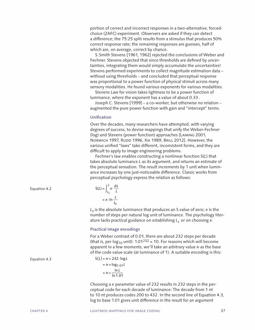
CHAPTER 4 LIGHTNESS MAPPINGS FOR IMAGE CODING 37
portion of correct and incorrect responses in a two-alternative, forced-choice (2AFC) experiment. Observers are asked if they can detect a difference; the 75:25 split results from a stimulus that produces 50% correct response rate; the remaining responses are guesses, half of which are, on average, correct by chance.
S. Smith Stevens [1961, 1962] rejected the conclusions of Weber and Fechner. Stevens objected that since thresholds are defined by uncer-tainties, integrating them would simply accumulate the uncertainties! Stevens performed experiments to collect magnitude estimation data – without using thresholds – and concluded that perceptual response was proportional to a power function of physical stimuli across many sensory modalities. He found various exponents for various modalities.
Stevens Law for vision takes lightness to be a power function of luminance, where the exponent has a value of about 0.33 .
Joseph C. Stevens [1999] – a co-worker, but otherwise no relation – augmented the pure power function with gain and “intercept” terms.
Unification
Over the decades, many researchers have attempted, with varying degrees of success, to devise mappings that unify the Weber-Fechner (log) and Stevens (power function) approaches [Laming 2001, Norwich 1997, Rudd 1996, Xie 1989, Brill 2012]. However, the various unified “laws” take different, inconsistent forms, and they are difficult to apply to image engineering problems.
Fechner’s law enables constructing a nonlinear function S(L) that takes absolute luminance L as its argument, and returns an estimate of the perceptual sensation. The result increments by 1 unit when lumin-ance increases by one just-noticeable difference. Classic works from perceptual psychology express the relation as follows:
S(L) = k ·dLLLz
L
= k ·lnLLz
Equation 4.2
Lz is the absolute luminance that produces an S value of zero; k is the number of steps per natural log unit of luminance. The psychology liter-ature lacks practical guidance on establishing Lz or on choosing k.
Practical image encodings
For a Weber contrast of 0.01, there are about 232 steps per decade (that is, per log10 unit): 1.01232 = 10. For reasons which will become apparent in a few moments, we’ll take an arbitrary value n as the base of the code value scale (at luminance of 1). A suitable encoding is this:
S L( ) = n + 232·logL
= n + log1.01L
= n +ln L
ln1.01
Equation 4.3
Choosing a k parameter value of 232 results in 232 steps in the per-ceptual code for each decade of luminance: The decade from 1 nt to 10 nt produces codes 200 to 432. In the second line of Equation 4.3, log to base 1.01 gives unit difference in the result for an argument

38 LIGHTNESS MAPPINGS FOR IMAGE CODING
ratio of 1.01. Few calculators compute log to arbitrary base; the third line shows a quotient of natural logs that yields the same result as 232 · log10 (or equivalently, log1.01 ). Here the natural log is used, but any ratio of logarithms having the same base is invariant to the base chosen, so any base would serve.
Figure 4.7 shows pure-log coding for n of 200, and plots a luminance range of 3 decades. Each decade can be coded in about 8 bits; for 3 or 4 decades, we need 10-bit coding.
A standardized example of pure log image coding is found in the MPEG and H.264 standards for digital video and high definition video (HD) [ISO/IEC 14496-2: 2004/Amd.3:2007]. Ordinarily, MPEG and H.264 represent R’G’B’ video signals where each component is raised to a power between 2.2 and 2.4 to produce display tristimulus val-ues. The amendment cited above provides an alternative scheme whereby parameters in MPEG’s Picture Display Extension signal use of a pure log code. A two-decade (100:1) luminance range is coded into eight bit component values 0 … 255; there are 127.5 codes per decade.9 For normalized video signal V in the range 0 to 1, decoding to tristimulus is represented as 10 2·(V − 1). For an 8-bit integer video signal value d from 0 … 255 and MPEG-coded, decoding is realized by 10 2/255 (d − 255). The Weber contrast is 10 2/255, about 0.018.10
MPEG prohibits negative values of V (or d ). With this pure-log code, luminance values less than 0.01 cannot be represented; a textbook encoder would clip them. The abrupt onset of clipping leads to objec-tionable image artifacts that a cinematographer would describe as
9 It is a pervasive design principle of MPEG that decoding and display are stan-dardized, not encoding. Surprisingly, the cited Amendment does not follow that principle: It expresses encoding, as V = 1.0 + 0.5 · log10 ( LC ). I follow the spirit of MPEG’s design principle: I describe the decoding of the pure-log code.
10 The cited amendment provides a second pure log code, where a 2.5-decade range of luminance values, about 316:1, is coded into 8-bit component values. There are 255/2.5 or 102 codes per decade. The additional 1/2-decade range is obtained at the expense of widening the Weber contrast to about 0.023.
0.001 0.01 0.1 1 10 100 1000
200
400
600
800
1000
Luminance, L [nt] (log scale)
Cod
e va
lue
Figure 4.7 Pure log coding for a Weber ratio of 1.01 is plotted, according to Equation 3. A range of absolute luminance from 1 to 1000 (three decades) produces code values 200 through about 900. There are 232 codes per decade.
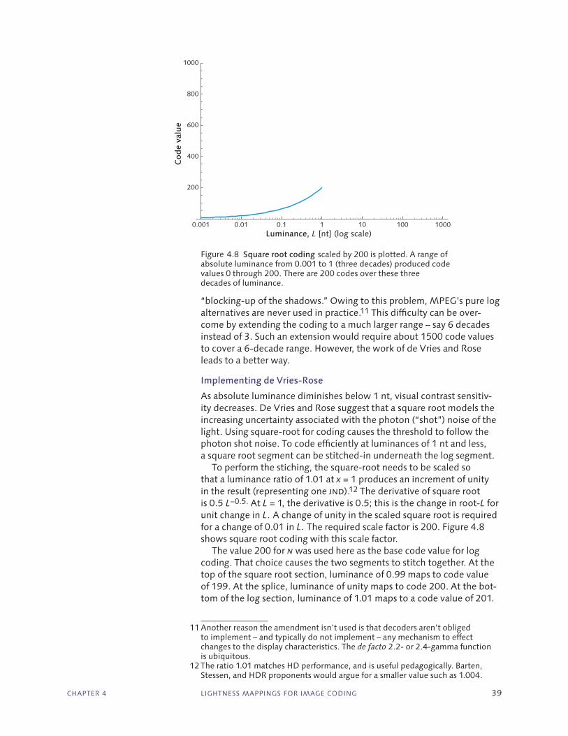
CHAPTER 4 LIGHTNESS MAPPINGS FOR IMAGE CODING 39
“blocking-up of the shadows.” Owing to this problem, MPEG’s pure log alternatives are never used in practice.11 This difficulty can be over-come by extending the coding to a much larger range – say 6 decades instead of 3. Such an extension would require about 1500 code values to cover a 6-decade range. However, the work of de Vries and Rose leads to a better way.
Implementing de Vries‑Rose
As absolute luminance diminishes below 1 nt, visual contrast sensitiv-ity decreases. De Vries and Rose suggest that a square root models the increasing uncertainty associated with the photon (“shot”) noise of the light. Using square-root for coding causes the threshold to follow the photon shot noise. To code efficiently at luminances of 1 nt and less, a square root segment can be stitched-in underneath the log segment.
To perform the stiching, the square-root needs to be scaled so that a luminance ratio of 1.01 at x = 1 produces an increment of unity in the result (representing one jnd).12 The derivative of square root is 0.5 L−0.5. At L = 1, the derivative is 0.5; this is the change in root-L for unit change in L. A change of unity in the scaled square root is required for a change of 0.01 in L. The required scale factor is 200. Figure 4.8 shows square root coding with this scale factor.
The value 200 for n was used here as the base code value for log coding. That choice causes the two segments to stitch together. At the top of the square root section, luminance of 0.99 maps to code value of 199. At the splice, luminance of unity maps to code 200. At the bot-tom of the log section, luminance of 1.01 maps to a code value of 201.
11 Another reason the amendment isn’t used is that decoders aren’t obliged to implement – and typically do not implement – any mechanism to effect changes to the display characteristics. The de facto 2.2- or 2.4-gamma function is ubiquitous.
12 The ratio 1.01 matches HD performance, and is useful pedagogically. Barten, Stessen, and HDR proponents would argue for a smaller value such as 1.004.
0.001 0.01 0.1 1 10 100 1000
200
400
600
800
1000
Luminance, L [nt] (log scale)
Cod
e va
lue
Figure 4.8 Square root coding scaled by 200 is plotted. A range of absolute luminance from 0.001 to 1 (three decades) produced code values 0 through 200. There are 200 codes over these three decades of luminance.
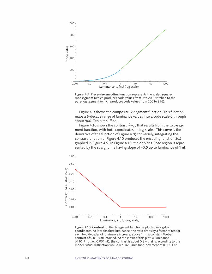
40 LIGHTNESS MAPPINGS FOR IMAGE CODING
Figure 4.9 shows the composite, 2-segment function. This function maps a 6-decade range of luminance values into a code scale 0 through about 900. Ten bits suffice.
Figure 4.10 shows the contrast, ΔL/L , that results from the two-seg-ment function, with both coordinates on log scales. This curve is the derivative of the function of Figure 4.9; conversely, integrating the contrast function of Figure 4.10 produces the encoding function S(L) graphed in Figure 4.9. In Figure 4.10, the de Vries-Rose region is repre-sented by the straight line having slope of −0.5 up to luminance of 1 nt.
0.001 0.01 0.1 1 10 100 1000
200
400
600
800
1000
Luminance, L [nt] (log scale)
Cod
e va
lue
Figure 4.9 Piecewise encoding function represents the scaled square-root segment (which produces code values from 0 to 200) stitched to the pure-log segment (which produces code values from 200 to 896).
0.001 0.01 0.1 1 10 100 1000
0.01
0.02
0.05
0.10
0.20
0.50
1.00
Luminance, L [nt] (log scale)
Co
ntr
ast,
ΔL/
L (lo
g sc
ale)
Figure 4.10 Contrast of the 2-segment function is plotted in log-log coordinates. At low absolute luminance, the ratio drops by a factor of ten for each two decades of luminance increase; above 1 nt, a constant Weber contrast of 0.01 is maintained. At the y-axis of this plot, a luminance of 10−3 nt (i.e., 0.001 nt), the contrast is about 0.3 – that is, according to this model, visual distinction would require luminance increment of 0.0003 nt.

CHAPTER 4 LIGHTNESS MAPPINGS FOR IMAGE CODING 41
The Weber-Fechner region beyond 1 nt is represented by the straight line having zero slope.
Returning to CIE L*, Figure 4.11 plots Weber contrast of the L* function, normalized for Yn at 100 nt. The y-axis is labelled ΔY/Y , to emphasize the fact that L* is based upon relative luminance not abso-lute luminance. Below relative luminance of about 0.01, L* has a linear segment; the Weber contrast has a discontinuity in its derivative at L* of 8. At the breakpoint, a unit step in L* corresponds to a Weber con-trast of 0.125. The fraction drops to 0.025 at reference white; it never reaches 0.01.
When luminance (L) and contrast ( ΔL/L ) are plotted in log-log coordinates, both segments of the L*(▪) function produce straight lines.
Direct coding of L* values from 0 to 100 is rarely if ever seen in practice; instead, the 0 to 100 range is scaled by 2.55 to yield a range 0 to 255 that is conveyed in 8-bits (for example, in Photoshop LAB format). In addition to L*, Figure 4.11 shows the 2.55 · L* code: The L* contrast curve just drops down by 0.4 log units, reaching very close to the 0.01 contrast at the maximum code value.
Medical imaging
Medical images are coded according to the DICOM series of stan-dards. The relationship of luminance values to greyscale image data is defined by the Grayscale Standard Display Function (GSDF) [ACR/NEMA PS 3.14 2009], to be detailed in Chapter 7, Analysis of greyscale medical image display, on page 81. Application-specific image data values are placed on a uniform perceptual scale bounded by the min-imum (Lmin) and maximum (Lmax) luminance available for a particular display.
Relative luminance, Y (log scale)
Co
ntr
ast,
∆L /L
(log
scal
e)
0.001 0.01 0.1 1 10 100 1000
0.01
0.005
0.02
0.05
0.10
0.20
0.50
1.00 L*
2.55 · L* (e.g., Photoshop LAB)
Figure 4.11 Weber contrast of L* is graphed for reference white (Yn) of 100 nt. The upper function represents coding with CIE L*, having 100 steps. The middle function represents CIELAB coding as used in 8-bit systems (such as Photoshop LAB), where L* values are multiplied by 2.55 to code into 8-bit integers ranging 0 through 255. The light dotted line is the 2-segment square root/pure log function of Figure 4.10.

42 LIGHTNESS MAPPINGS FOR IMAGE CODING
The GSDF mapping from absolute luminance L to jnd index value j is defined by the following rather unsatisfying eighth-degree polynomial in log10(L), having nine, eight-digit coefficients:
j( ) . . log ( ) . logL L= + ⋅ + ⋅71 498068 94 593053 41 91205310 1102
103
109 8247004 0 28175407( ) . log ( ) . log ( )L L L+ ⋅ + ⋅ 44
105
1061 1878455 0 18014349 0 1− ⋅ − ⋅ +. log ( ) . log ( ) .L L 44710899 0 01704684510
710
8⋅ − ⋅log ( ) . log ( )L L
Equation 4.4
Figure 4.12 presents a graph of this function. A graph of the Weber con-trast of the GSDF is presented in Figure 4.13.
Luminance, L [nt] (log scale)
JND
inde
x, j
0.1 1 10 100 10000
200
400
600
800
1000
Figure 4.12 DICOM GSDF coding is used in medical imaging. Absolute luminance from 0.05 nt to 4000 nt is mapped to a perceptually uniform scale (typically, integers) from 1 to 1023.
Figure 4.13 Weber contrast of the DICOM GSDF .
0.1 1 10 100 1000
0.01
0.02
0.05
0.10
0.20
0.50
Luminance, L [nt] (log scale)
ΔL/
L (lo
g sc
ale)
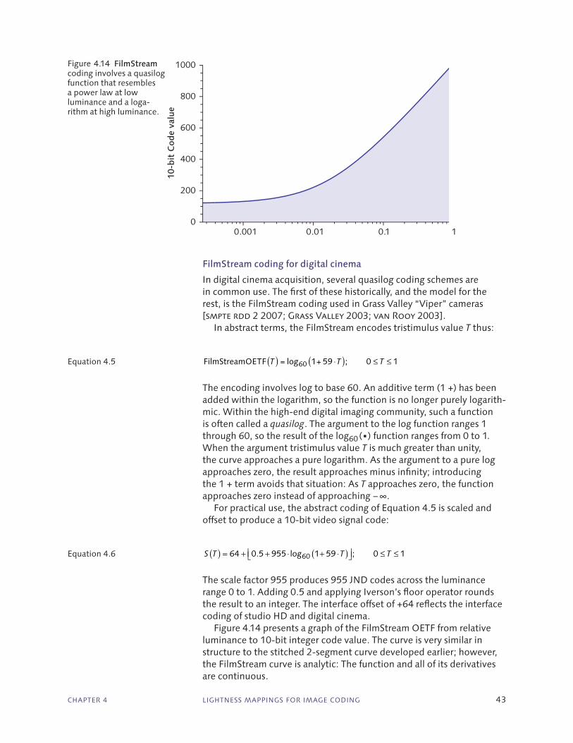
CHAPTER 4 LIGHTNESS MAPPINGS FOR IMAGE CODING 43
FilmStream coding for digital cinema
In digital cinema acquisition, several quasilog coding schemes are in common use. The first of these historically, and the model for the rest, is the FilmStream coding used in Grass Valley “Viper” cameras [smpte rdd 2 2007; Grass Valley 2003; van Rooy 2003].
In abstract terms, the FilmStream encodes tristimulus value T thus:
FilmStreamOETF T( ) = log60 1+ 59 T( ); 0 T 1Equation 4.5
The encoding involves log to base 60. An additive term (1 +) has been added within the logarithm, so the function is no longer purely logarith-mic. Within the high-end digital imaging community, such a function is often called a quasilog. The argument to the log function ranges 1 through 60, so the result of the log60 (▪) function ranges from 0 to 1. When the argument tristimulus value T is much greater than unity, the curve approaches a pure logarithm. As the argument to a pure log approaches zero, the result approaches minus infinity; introducing the 1 + term avoids that situation: As T approaches zero, the function approaches zero instead of approaching − ∞.
For practical use, the abstract coding of Equation 4.5 is scaled and offset to produce a 10-bit video signal code:
S T( ) = 64 + 0.5 + 955 ⋅ log60 1+ 59 ⋅T( )⎢⎣ ⎥⎦; 0 ≤ T ≤ 1Equation 4.6
The scale factor 955 produces 955 JND codes across the luminance range 0 to 1. Adding 0.5 and applying Iverson’s floor operator rounds the result to an integer. The interface offset of +64 reflects the interface coding of studio HD and digital cinema.
Figure 4.14 presents a graph of the FilmStream OETF from relative luminance to 10-bit integer code value. The curve is very similar in structure to the stitched 2-segment curve developed earlier; however, the FilmStream curve is analytic: The function and all of its derivatives are continuous.
0.001
Relative luminance, Y (log scale)
10-b
it C
ode
valu
e
0.01 0.1 1
200
0
400
600
800
1000Figure 4.14 FilmStream coding involves a quasilog function that resembles a power law at low luminance and a loga-rithm at high luminance.
44 LIGHTNESS MAPPINGS FOR IMAGE CODING
A comparable code was developed by Silicon Imaging for the SI 2K camera. (SI cameras were used to acquire major portions of the movie Slumdog Millionaire.) The coding is called SI log90 ; encoding from tris-timulus value T to the abstract range 0 to 1 takes this form:13
SIlogOETF T( ) = log90 1+ 89 T( ); 0 T 1Equation 4.7
Like FilmStream, the abstract code is scaled and offset for practical use. Following from the FilmStream and SI log90 codes, during the past
15 years many more log-based OETFs for D-cinema acquisition have been commercialized. Most of the commercially deployed systems have published equations, owing to the necessity to invert the camera encoding function in the early stages of most post-production pipelines (and all postproduction pipelines that involve computer-generated imagery and visual effects, CGI/VFX). Despite the published functions, no standards have emerged. Little information is available concern-ing the origin of the parameters of these curves, though they all have roughly the shape that I have described.
The 2-segment square root/log function was presented on a scale of absolute luminance values from 10 −3 to 103 nt. When quasilog func-tions such as FilmStream or SI log90 are used to acquire image data, sensor values are scaled, typically by the cinematographer or video camera operator who sets exposure such that unity represents the max-imum value that can be coded without clipping.
The FilmStream and SI log90 quasilog curves emerged from pragmatic engineering concerns associated with high-quality image acquisition. However, in my view they represent an excellent match to the demands of the human visual system, approaching power law behaviour at low luminance and approaching log behaviour at high luminance.
Summary
The Weber-Fechner and Stevens empirical “laws” are both widely used without reference to adaptation or absolute luminance level. However, adaptation matters, and absolute luminance matters. Different models of vision are applicable in different absolute luminance regimes. The de Vries-Rose power-function “law” models the visual contrast thresh-old well at low luminances, below about 0.1 nt. The Weber-Fechner “law” models the visual contrast threshold well at high luminances, above about 0.1 nt.
Chapter 3, Perceptual uniformity in digital imaging, showed that 8-bit R′G′B′ components suffice for distribution of image data covering a limited contrast range, up to 320:1 or so. However, it is clear from Chapter 3 that 10-bit R′G′B′ components produce Weber fraction far lower than the 0.01 or so that satisfies the human visual requirement of avoiding detectable banding. The analysis of the present chapter makes clear that codewords above 200 or so are most effectively used if they are based upon a logarithmic OETF (or an exponential EOTF).
Quasilog image encoding schemes match well the requirements of de Vries-Rose at low luminance and Weber at high luminances.
13 The SI log90 format is not publicly documented apart from passing mention in a web forum posting [Newman 2007].

45
5 Appearance transforms in
video/HD/UHD/D‑cinema
The case for the primacy of the mastering display in the determination of faithful presentation was made in Chapter 2, Image acquisition and presentation. In the present chapter, that notion is formalized as Axiom Zero. The associated mastering‑display‑referred image state was intro-duced in Chapter 2; this chapter presents the details. Chapter 2 also provided a brief description of the scene-referred image state, and it contained a brief description of the (generalized) display-referred image state. In the present chapter those concepts are detailed.
Chapter 3, Perceptual uniformity in digital imaging, described how perceptually uniform coding enables perceptually efficient image coding. Acceptance of Axiom Zero implies that perceptual uniformity is critical in distribution. The present chapter clarifies the idea.
The concept of image state was formalized in the period 1985 – 1995 during the development of colour management systems for prepress. Those systems evolved into general-purpose desktop computer col-our management systems (CMSs). In due course a standards body was established (International Colour Consortium, ICC) and standards were agreed upon and promulgated [ICC 1:2010; ISO 15076]. The ICC tech-niques and standards were conceived for the faithful presentation of hard-copy reflectance prints in graphic arts.
Despite appearance issues being recognized and handled in the signal processing of graphic arts systems, video technologists remain largely ignorant of appearance effects, and they discount the require-ment for their compensation. Even modern video texts [Tooms 2016; see Poynton 2017] describe the ideal of linear-light processing end-to-end, and have hand-waving descriptions of the alterations to linear processing that are fundamentally necessary in practice.
The present chapter identifies the rather curious scheme by which traditional video/HD systems accomplish appearance mapping. There is no specific block in the block diagram that imposes the correction, so the correction has for decades gone unnoticed by video theorists.
HDR video systems accomplish appearance compensation, but mainly through proprietary schemes that are not documented in the open literature. This chapter invokes the concept of optical‑to‑optical transfer function (OOTF) to describe HDR appearance compensation, but contrary to previous work this chapter argues that not one but three distinct OOTFs are needed.

46 APPEARANCE TRANSFORMS IN VIDEO/HD/UHD/D-CINEMA
sRGB coding
Figure 5.1 sketches a simple sRGB imaging system, comprising a cam-era, a “channel,” and a display. The sRGB standard [IEC 61966-2-1] specifies that the EOTF shall be a 2.2-power function.1 An sRGB dis-play’s “gamma” is said to be 2.2.
For image data generated synthetically and presented to an sRGB display, at first glance the situation is clear: Produce whatever data val-ues are required to drive the display to present the intended colours.
For sRGB image data to be produced by a camera, the assumption is commonly made that the camera should have an OETF that is the inverse of sRGB’s EOTF. Figure 5.1 includes a putative OETF that is a 1/2.2-power function.
Despite the intuitive appeal of this approach, it is almost always wrong. There is an unstated assumption in such sketches that pres-entation luminance values are expected to be proportional to scene luminance values. Although the scheme of Figure 5.1 conveys rela‑tive luminance values accurately, the display very rarely has the same absolute light level as that of the scene: The scene ordinarily has much higher absolute luminance. Light level affects the human viewer through what are termed colour appearance effects. To analyze even the sRGB case, we must explore colour appearance.
Colour appearance
According to CIE [17.4], colour appearance is the “aspect of visual perception by which things are recognized by their colour.” Colour is in the human eye and brain; it is not a completely physical phenomenon. Colour appearance, as used in digital imaging, refers to the variability of perceived colour of a physical stimulus (target), or its portrayal on a dis-play, taking into account aspects of the visual stimulus and elements surrounding it in the visual field, including absolute luminance, object shape, angular subtense, visible texture, and spatial frequency.
It has been known for more than half a century that as illumination decreases, colourfulness decreases (the Hunt effect) and visual con-
1 The sRGB standard has complexities concerning a linear segment near black. We disregard these complexities for now. Also, the standard states that refer-ence (peak) display luminance shall be 80 nt, when in fact modern displays are typically set for white of about 320 nt. We disregard this fact for now as well.
scen
e
sRGBOETFV = T 1/2.2
sRGBEOTFT = V 2.2
pres
enta
tio
n
putative!
Figure 5.1 sRGB digital image data is intended be displayed with a 2.2-power EOTF. At the left, light (signified by a dotted line) enters a camera; at the right, light is emitted by a display. T symbolizes tristimuli; V symbolizes video signal. It is widely – and generally incorrectly – assumed that correct imaging is achieved when scene and presentation light levels are proportional: It is assumed that the proper OETF to encode sRGB image data is the mathematical inverse of decoding and display. For sRGB, the correct camera OETF is presumed to be a 1/2.2-power function. That approach is nearly always wrong, because a real scene usually has diffuse white luminance higher than the display (or, if the scene is imaginary, is intended to portray an environment brighter than the viewers’ environment). The naïve approach to sRGB OETF would lead to presentation having lower contrast and less colourfulness than expected.

CHAPTER 5 APPEARANCE TRANSFORMS IN VIDEO/HD/UHD/D-CINEMA 47
trast – or “contrastiness” – decreases (the Stevens effect). These effects alter the appearance of coloured images. The ratio of average scene or image luminance to surround luminance also plays a role. Visual adap-tation has a dominant effect on appearance. Visual adaptation is mainly controlled by a spatiotemporal average of absolute luminance: direct light sources and specular highlights do not contribute significantly to average luminance, and thus do not significantly influence adaptation.
In cinema, video/HD, and HDR, we often seek to recreate – on a rather dark display, often in a dark environment – the appearance of a bright scene. Compensation for appearance effects is necessary.
There is often a ratio of 100 or more in absolute luminance between diffuse white in a scene and its portrayal on a studio reference dis-play at ingest or at mastering. For example, a white card outdoors on an overcast midday could reflect 10 000 nt (in photographic terms, about LV 15). On a clear midday, diffuse white luminance could reach 32 000 nt (LV 16 2/3).2 In HD mastering this would typically be por-trayed at about 80 or 100 nt. Even in HDR, portrayal of diffuse white should be at a luminance that lies below the onset of power limiting, say 200 nt for a 1000 nt master, otherwise the portrayed image is liable to “pulse” as the scene gets brighter and darker.
Robert W.G. Hunt first described [1952], and amplified in many papers and books, that (visual) colourfulness3 decreases as illumina-tion decreases. Physical chroma, tristimuli, and relative luminance are unchanged.
S. Smith Stevens described [1960] that visual contrast (“contrasti-ness”) decreases as illumination decreases. Again, physical contrast, tristimuli, and relative luminance are unchanged.
C. James Bartleson and Edwin J. Breneman described [1967] that a dark surround alters the apparent tone and colour scale of an image: the darker the surround, the less the visual colourfulness and visual contrast. Surround is most usefully expressed as a fraction of the dif-fuse white luminance experienced by the viewer. An ordinary scene has a relative luminance of around 15 – 18% (“mid grey”); when the visual context of a scene is comparable to the scene itself, the viewing situation is described as average surround. Typical consumer viewing is described as dim surround,at about 5%. HD mastering as usually practiced has a very dim surround of about 1%. (Certain professional standards call for HD and HDR mastering at 5% surround; however, this is well outside normal studio practice.) Cinema viewing takes place in a dark (0%) surround.
The Hunt, Stevens, and Bartleson-Breneman effects are all percep-tual; they are not predicted or described by physics or by classical color-imetry, and they cannot be measured by instruments. The effects have been studied in modern colour appearance theory; they are described in textbooks such as those by Giorgianni [2008] and Fairchild [2013]; they are incorporated into modern colour appearance models such as CIECAM02 and CAM16 [Li 2017].
2 Light value (LV) in photography is computed as 10/3 · log10 (0.4 · E ), where E is illuminance in lux. Illuminance of 2.5 lx has LV 0. For a 90% diffuse white reflector, light value is 10/3 · log10 (3.49 · L ), where L is luminance in nt.
3 I use colourfullness instead of saturation; the latter is an ambiguous term that could refer to clipping of a sensor channel or a signal component channel.

48 APPEARANCE TRANSFORMS IN VIDEO/HD/UHD/D-CINEMA
Picture rendering is a general term that refers to signal processing that compensates for appearance effects.4 Given that description, we can return to the colour image processing pipeline.
Highly simplified pipeline
Figure 5.2 sketches a camera and a display, but now calling out (at the left) the absolute luminance values of diffuse white (Ldw ) in various scene acquisition situations ranging over a 10 000:1 ratio of lumin-ance values. At the right, absolute luminance values of diffuse white as portrayed (Ldwp ) in various display situations is indicated, ranging over a 10:1 ratio from the 32 nt white typical in conventional cinema to 320 nt typical in a computer (PC) display or a consumer electronics television display.
Program acquisition has a diversity of scene conditions; program viewing has a diversity of display condition. Program production requires decision about mastering. It is standard in HD [SMPTE 2080-1] to have reference white at 100 nt. HD mastering displays are typically viewed in a 1% (“very dim”) surround.5 In HD production, a standard HD mastering display in a standard viewing condition is taken as the
4 Rendering intent is a graphic arts term; it differs from picture rendering. Render‑ing intent is not an appropriate term for digital cinema, video/HD, and HDR.
5 SMPTE ST 2080-3 calls for a surround luminance of 5 nt (that is, 5% of the 100 nt reference white luminance of ST 2080-1). ST 2080-3’s Annex A provides a highly questionable methodology for establishing the 5 nt value; there is no mention of the standards group taking any measurements. In 2010, I visited four Blu-ray mastering studios (three in Los Angeles and one in New York), and I measured surround values averaging about 1 nt. It was an explicit criterion during the development of the BT.1866 EOTF for HD to codify existing practice; to do otherwise would “break the vault” in the sense that archived material taken out of the vault and displayed in BT.1886 would change in appearance compared to the appearance of the material at the time it was put into the vault. Evidently, no such consideration was applied to the development of SMPTE ST 2080-3. I urge ignoring the 5 nt surround provision of ST 2080-3.
Picture RenderingTransform
scen
e
PC/consumer tvstudio HDcinema (“2D”)
320 nt100 nt32 nt
bright daylight
overcast daylight
studio/bright interior
dim interior
ten candles at 1 m
one candle at 1 m
32,000
3,200
320
32
3
0
nt
nt
nt
nt
.2 nt
.32 nt
Ldw
Ldwp
pres
enta
tio
n
Camera Display
Scene condition
Display condition
Figure 5.2 A picture rendering transform must be interposed between camera and display in the usual case that light levels differ between acquisition and presentation, in order to preserve appearance. On the left is a representation of a range of scene luminance values reflected from a perfect diffuse white reflector in logarithmically spaced intervals a decade apart (overall, a 10 000:1 range). On the right are three absolute luminance levels typical of the portrayal (presentation) of diffuse white, a range of 10:1.

CHAPTER 5 APPEARANCE TRANSFORMS IN VIDEO/HD/UHD/D-CINEMA 49
“hinge point” between diverse scene conditions and diverse pres-entation conditions. The standardization of mastering allows picture rendering to be separated into two components, scene rendering and display rendering. A potential m × n combinations are thereby reduced to m + n. If we assume that scene rendering requires a set of parameters each decade, and display rendering requires a set each half-decade, 6 × 3 = 18 combinations in this example are reduced to 9.
Scene rendering then is signal processing to compensate for the visual appearance effects between the scene and the mastering display. We say “mastering display,” but in complex post-production and digital intermediate (DI) pipelines the complexity is reduced if the image at ingest roughly matches the appearance of the scene; consequently, post/DI image viewing typically takes place after some sort of rendering that is typically very similar or perhaps identical to the scene rendering for mastering. (However, this approximate appearance match at ingest is not a constraint of the mastered program.)
Consumer video displays and their viewing conditions rarely match those of video mastering; these differences introduce appearance shifts that must be compensated. Display rendering is signal processing to compensate for the appearance effects associated with diverse con-sumer display luminance levels and surround conditions. The goal of display rendering is to match, in the eyes of the consumer, the appear-ance of the mastering display.
In cinema, exhibition to consumers is accomplished with display and viewing conditions effectively identical to those at mastering. Recreat-ing the physical stimulus of colour suffices, and no display rendering is necessary or desirable.
Figure 5.3 sketches the previously presented camera and display, but now with the picture rendering transform partitioned into scene rendering and display rendering components.
Scene RenderingTransform
scene
PC/consumer tvstudio HDcinema (“2D”)
320 nt100 nt32 nt
bright daylight
overcast daylight
studio/bright interior
dim interior
ten candles at 1 m
one candle at 1 m
32,000
3,200
320
32
3
0
nt
nt
nt
nt
.2 nt
.32 nt
LDW
mastering
presentationCamera Mastering
Display
DisplayDisplayRenderingTransform
Figure 5.3 Scene and display conditions are independent. Scene conditions and display conditions both affect picture rendering. However, program creators seek to master in a single condition. Diffuse white in HD is ordinarily portrayed at absolute luminance close to the luminance of reference white. A scene rendering transform accommo-dates diverse scene conditions; a display rendering transform accommodates display conditions different from mastering. The sketch is reminiscent of Figure 1 of Pindoria [2016] and Figure 1 of Thomson et al. [2017]; however, my functional labels are different than theirs.

50 APPEARANCE TRANSFORMS IN VIDEO/HD/UHD/D-CINEMA
Definition of scene‑referred
For image data that is acquired from or otherwise intimately connected to a scene, scene‑referred is the property of having a documented mathematical mapping from estimated colorimetric light (e.g., absolute or relative luminance, or tristimuli) to image signal value.6 In absolute scene-referred image data, image signal values or associated metadata convey estimated absolute luminance in the scene, such as the relation between signal value and the absolute luminance of an 18%, 90%, or other diffuse reflector in the scene under the dominant scene illumin-ant. A variation is relative scene‑referred, where image signal values con-vey estimated relative luminance. Image data cannot be scene referred if any of the following conditions hold:
[a] camera tone or colour mapping algorithms are unknown or undocumented;
[b] camera adjustments (apart from exposure or gain) are made without being accompanied by documented algorithms and associated metadata; or
[c] camera signal processing imposes significant gamut limitations with respect to the Pointer [1980] gamut, such as clipping to BT.709 gamut.
In digital photography, scene-referred image signal values are called raw: Image signal values are absent any scene or display rendering transforms. Raw image data may be radiometric or processed by a non-linear OETF, and may be uncompressed or compressed. Raw data is typically in mosaic (“Bayer”) form, but may be demosaicked.
Definition of display‑referred
Display‑referred describes image data wherein intended appearance is obtained through a documented mathematical mapping from signal value to absolute colorimetric light at the surface of a particular display viewed in a particular, specified viewing condition.7
In mastering‑display‑referred image data, intended appearance is obtained, or creative decisions are finalized, through a documented mathematical mapping from signal value to absolute colorimetric light at the surface of a standardized display as viewed in a particular speci-fied or standardized viewing condition.
6 Image signal value may be referenced to the scene directly, or may be refer-enced to the image (focal) plane of the sensor, in which case optical flare may be incorporated.
7 FilmLight Ltd is a highly respected developer of digital filmmaking equipment, including colour grading systems. The company’s Baselight grading system has a highly advanced DI pipeline, including rendering transforms. Its system archi-tecture involves a colour transform that allows parameterized scene conditions and parameterized mastering display conditions. The Baselight scene-to-mas-tering transform is called display rendering transform (DRT). A scene-to-master-ing transform potentially covers a luminance ratio of up to 10 000:1; potential diversity in mastering display luminance (whether diffuse white or average) is perhaps just 10:1. Because the scene-to-mastering transform is by far the dominant transform, I call it a scene rendering transform instead of a display rendering transform. However, my discrepancy with FilmLight terminology is unfortunate.

CHAPTER 5 APPEARANCE TRANSFORMS IN VIDEO/HD/UHD/D-CINEMA 51
Scene rendering in HD
Now that scene rendering and display rendering have been introduced and defined, we can examine how scene rendering is accomplished in HD video.8 The situation has confused video engineers for decades because there is no explicit scene rendering block or display rendering block in any classic video system block diagram.
Consider the usual case of a bright scene in an average surround condition, portrayed on a somewhat darker display in a somewhat darker surround. Scene rendering has to increase physical contrast (to compensate the loss of visual contrast owing to the Stevens effect), to increase physical chroma (to compensate loss of colourfulness owing to the Hunt effect), and to increase both physical contrast and physical chroma (to compensate the loss of visual contrast and colourfulness owing to the surround effect).
Physical contrast can be increased by simply scaling lightness, exemplified by CIE L* lightness: Consider stretching the lightness scale by multiplying each L* increment by 1.2. This act has an effect on large contrast ranges: a 50-unit excursion in L* values becomes 60 units.
In video acquisition, scene tristimuli are subject to the camera OETF. Examination of the BT.709 OETF standard for HD reveals a very close fit to a 0.5-power function (that is, BT.709 approximates a square root). Scaling the square root (or indeed any power function of luminance) by a factor of 1.2 is mathematically equivalent to applying a 1.2-power function to the original (luminance) quantity. In HD, a pure 2.4-power EOTF is standard. A 1/2.4 (approximately 0.42) power applied as an OETF would yield display tristimuli proportional to the scene. However, BT.709 applies an effective 0.5-power instead. The 0.5-power OETF and the 2.4-power compose as equivalent to a 1.2-power function through the OETF and the EOTF. This amazingly simple scheme imposes the standard, baseline scene rendering transform of HD: It is a power function having an exponent of 1.2.
The BT.709 standard (or “factory”) setting is such that pleasing images are portrayed on 100 nt display when scene diffuse white luminance is about 3200 nt. If the scene luminance is higher than 3200 nt, then more compensation will be necessary. In a mastering-dis-play-referred system, the mastering EOTF is fixed; the compensation obviously belongs at the camera. The experience of cinematographers, directors of photography (DoPs), and HD camera operators suggests that a 32 000 nt scene requires camera OETF equivalent to about a 0.55-power instead of 0.5. If the scene luminance is lower than 3200 nt, then less scene rendering compensation will be necessary. Anecdotal evidence suggests that a 320 nt scene produces pleasing images on an HD mastering display using camera OETF equivalent to about a 0.45-power instead of 0.5. A dim interior might be acquired using camera OETF equivalent to about a 0.4-power.
DoPs and HD camera operators are very familiar with adjusting camera “gamma” to yield pleasing pictures for particular scene light-ing conditions. However, they may find the gamma numbers quoted above – 0.55 for a bright sunlit scene, 0.5 as a baseline for a scene lit by overcast daylight, 0.45 for a studio scene, and 0.4 for a dim interior – to be somewhat high. The DoP or camera operator may expect 0.5, 0.45,
8 I say “HD,” but the approach was used in SD and even in analog video.

52 APPEARANCE TRANSFORMS IN VIDEO/HD/UHD/D-CINEMA
0.4, and 0.35 respectively. The apparent dilemma is resolved by recog-nizing that camera gamma variations are not labelled by the effective gamma; instead, they are labelled by the exponent of the OETF’s power function prior to scaling and offsetting associated with insertion of the linear segment near black. Details of the formulation of the BT.709 OETF are described by Poynton [2012, Ch. 27]. Gamma settings on commercial HD cameras are designated (or, if you will, “advertised”) by a number roughly 0.05 smaller than the effective power.
Figure 5.4 depicts the expansion of the scene luminance range by the application of the 1.2-power scene rendering transform, in this example taking 3 decades of scene luminance to 3.6 decades of mastering dis-play luminance.
We can now return to the HD pipeline. Figure 5.5 sketches the cam-era and display seen in previous figures, but now augmented by a phan-tom block that represents the implicit scene rendering power function. Scene luminance of 3200 nt, equivalent to overcast daylight, is high-lighted; this is the scene luminance best compensated by the standard BT.709 “factory” setting of an HD camera. The 1.2-power rendering takes image appearance from the 320 nt scene to a 100 nt display, a ratio of 32:1. Cinema display (at 32 nt) will require display rendering, as will PC display or consumer television display (at perhaps 320 nt) .
Chroma compensation
Scene rendering in HD was introduced by describing how a mild power function, having an exponent slightly greater than unity, is applied to luminance. The explanation as set out above is correct for the greyscale, where R = G = B. Contrast is increased. However, scene rendering also requires an increase in physical (or if you wish, colorimetric) chroma. Once video is encoded using the Y′CBCR technique, chroma could be increased simply by applying a small amount of gain (perhaps 1.2) to the CBCR components. However, a simpler method is possible, and in fact preferable: Scene rendering is implemented by applying the mild power function on individual RGB tristimuli components instead of on lumin-
10 000
32 000Scene Absolute luminance
of diffuse white,LDW [nt] (log scale)
1000
100
10
0.01
1
0.1
3 de
cade
s in
sce
ne,
L DW
320
0 nt
(20
% s
urro
und) Ingest
100
1000
10
0.01
1
0.1
3.6
deca
des
at H
D m
aste
ring
, L D
W 1
00 n
t (1
% s
urro
und)
1.2expand
Figure 5.4 Basic scene rendering in HD . Luminance levels of an example scene are depicted, with absolute luminance of diffuse white (Ldw) at 3200 nt, a decade below the maximum of 32 000 nt under bright sunlight. A 3-decade range (1000:1) is sketched. HD mastering display absolute luminance is on the right, with diffuse white portrayal at 100 nt. Scene luminance is reduced overall by a factor of 32:1 in transfer to the mastering display. Luminance ratios in the scene need to be expanded to overcome the Hunt, Stevens, and surround effects. For 100 nt diffuse white in the very dim (1%) surround of HD mastering, preserving appearance of 3200 nt white in an average surround requires that luminance ratios be scaled by a factor of 1.2. In log space, the transform is just scaling by 1.2; in “linear-light” space, it’s a 1.2-power function. The 1000:1 luminance range of this scene (3 decades) expanded to 4000:1 (3.6 decades) at mastering (1000 1.2 = 4000).

CHAPTER 5 APPEARANCE TRANSFORMS IN VIDEO/HD/UHD/D-CINEMA 53
ance. If R−G, R−B, or G−B colour difference values were to be formed, they would all be zero on the greyscale (where R = G = B). When any colour difference departs from zero – that is, off the greyscale axis – the power function on each component causes the colour difference to be amplified. The effect is a moderate chroma increase in the midscale, reducing to no amplification at the primaries or secondaries.
Axiom Zero revisited
Previous sections have outlined a systematic approach to scene render-ing in HD. However, the primacy of the mastering display, introduced as Axiom Zero in Chapter 2, Image acquisition and presentation, must now be reëmphasized. In the making of art – in our case, colour images – what matters is what is perceived. Any image data transformation that yields the desired image at mastering is correct by definition, no mat-ter what science was or was not used to get there. The video industry has survived without a clear systematic approach to scene rendering because cinematographers, DoPs, and camera operators have felt free to adapt the camera parameters in any way that seemed appropriate to produce the intended image without any necessary reference to colour appearance science. If the imagery at post-production ingest was deemed unsatisfactory, then the colourist would make whatever signal alterations were necessary to achieve the desired appearance at mastering.
Historically, and in most applications of HD today, video signal manipulation was accomplished in the “gamma-corrected” mas-tering-display-referred domain. Owing to the likelihood of signal manipulation at acquisition (as just mentioned), HD image signals typically lack any objective connection to scene luminance levels (either absolute or relative).
scen
e
PC/consumer tvstudio HDcinema (“2D”)
320 nt100 nt32 nt
32,000
3,200
320
32
3
0
nt
nt
nt
nt
.2 nt
.32 nt
LDW
pres
enta
tio
n
BT.709OETFV = T 0.5
BT.1886EOTFT = V 2.4
bright daylight
overcast daylight
studio/bright interior
dim interior
ten candles at 1 m
one candle at 1 m
Implicit 1.2-powerscene renderingtransform
32:1 ratio
Figure 5.5 Scene rendering in HD is not implemented in any single processing block. The EOTF of studio HD is standardized in BT.1886 as an effective 2.4-power function. The OETF of HD is standardized in BT.709 as effectively a square root. Obviously, these are not inverses. The composition of the standard OETF and EOTF is equivalent to a 1.2-power function on each of the R, G, and B tristimuli. That 1.2-power function imposes HD’s scene rendering transform. The 1.2-power is appropriate for a scene at diffuse white of about 3200 nt and portrayal of that diffuse white on the mastering display at 100 nt. Scenes having diffuse white considerably brighter than 3200 nt need more correction than the 1.2-power; scenes having diffuse white less luminous than 3200 nt need less correction.

54 APPEARANCE TRANSFORMS IN VIDEO/HD/UHD/D-CINEMA
Many modern productions have computer-generated imagery (CGI) and/or visual effects (VFX), where synthetic image elements are com-bined with “live action footage.” In these cases, inversion of the OETF is necessary to obtain scene-referred signal values. A later section of this chapter will describe the ACES system that has been standardized and widely deployed to address such needs.
Display rendering
As outlined earlier in this chapter, HD display rendering is referenced to the studio reference display, which according to BT.1886 closely approximates a pure 2.4-power function, according to ST 2080-1 delivers 100 nt reference white, and according to industry practice has surround of 1% of diffuse white.
Consider displaying such HD imagery on a home theatre projector that portrays diffuse white at 32 nt, in a completely dark (0%) surround. The projected diffuse white has lower luminance than at mastering, and the surround luminance is lower than mastering. Hunt, Stevens, and surround effects are more pronounced than at mastering. Compensa-tion of these effects can be achieved by using a 2.6-power EOTF instead of 2.4. Display rendering is characterized a power-function having an exponent of about 2.6/2.4 = 1.1. The situation is sketched in the “1.1 expand” portion of Figure 5.6.
Figure 5.6 Basic display rendering in HD is sketched above, to the right of a copy of Figure 5.4. Mastering luminance is on the left; home theatre display luminance is at the centre; and consumer display luminance is at the right. In display rendering for home theatre, luminance ratios at HD mastering are expanded in order to overcome the Hunt, Stevens, and surround effects. For white at 32 nt in a dark (0%) surround, preserving appearance requires scaling luminance ratios by a factor of 1.1; a 1000:1 range of HD mastering luminance is expanded to 2000:1 at the home theatre display. A 1.1-power display rendering function results. For consumer display, with white at 320 nt in an average (15 – 18%) surround, preserving appearance requires reducing HD mastered luminance ratios by a factor of 0.9; a 1000:1 range of mastering luminance is reduced to 500:1 at the consumer display. A 0.9-power display rendering function results.
10 000
32 000Scene Absolute luminance
of diffuse white,LDW [nt] (log scale)
1000
100
10
0.01
1
0.1
3 de
cade
s in
sce
ne,
L DW
320
0 nt
(20
% s
urro
und) Ingest
100
1000
10
0.01
1
0.1
3.6
deca
des
at H
D m
aste
ring
, L D
W 1
00 n
t (1
% s
urro
und)
1.2expand
0.9compress
1.1expand
100
1000
10
0.01
1
0.1 Cin
ema
disp
lay,
L D
W 3
2 nt
(0%
sur
roun
d)
100
1000
10
0.01
1
0.1 Con
sum
er d
ispl
ay,
L DW
320
nt
(5%
sur
roun
d)
100
1000
10
0.01
1
0.1 Mas
teri
ng d
ispl
ay,
L DW
100
nt
(1%
sur
roun
d)
Homecinema
Consumer/PC displayMastering

CHAPTER 5 APPEARANCE TRANSFORMS IN VIDEO/HD/UHD/D-CINEMA 55
Consider displaying HD imagery on a brighter display in a brighter environment than HD mastering, for example a typical sRGB display (with reference/diffuse white about 320 nt in a 15 – 18% average sur-round), or consumer video display (with similar luminance but a 5% dim surround). Hunt, Stevens, and surround effects are less pronounced than at mastering. Correct appearance can be achieved by using a dis-play power-function exponent (“gamma”) of around 2.2 (as opposed to 2.4 at mastering). The implicit display rendering function is thereby a power-function having an exponent of about 2.2/2.4 = 0.9, the “0.9 compress” portion at the right of Figure 5.6.
The example above described home theatre projection of imagery mastered in HD conditions. “Gamma” of 2.6 was appropriate. Mas-tering and presentation of native digital cinema (d-cinema) material, though, is mastered with an EOTF comprising a pure 2.6-power func-tion [SMPTE ST 431-1, SMPTE RP 431-2].9 D-cinema display charac-teristics and viewing conditions at presentation (“exhibition”) closely match display and viewing conditions at mastering. In d-cinema, display rendering is neither required nor desirable.
Like HD, d-cinema is completely mastering-display-referred. SMPTE D-cinema standards make no reference whatsoever to the scene-re-ferred image state or to scene rendering. (However, the emergent ACES system, to be described in a few moments, involves scene-referred image data.)
Scene rendering in sRGB
We can now return to the basic sRGB block diagram of Figure 5.1 (on page 46, at the start of this chapter). Figure 5.7 augments that figure with a phantom block showing the implicit picture rendering transform that is imposed on HD material when displayed with “gamma 2.2”.
9 The standard d-cinema display primary set, denoted DCI P3, has a somewhat wider gamut than the BT.1886 HD primary set.
scen
e
PC/consumer tvstudio HDcinema (“2D”)
320 nt100 nt32 nt
LDW
pres
enta
tio
n
BT.709OETFV = T 0.5
sRGBEOTFT = V 2.2
32,000
3,200
320
32
3
0
nt
nt
nt
nt
.2 nt
.32 nt
bright daylight
overcast daylight
studio/bright interior
dim interior
ten candles at 1 m
one candle at 1 m
Implicit 1.1-powerpicture renderingtransform
10:1 ratio
Figure 5.7 Picture rendering in sRGB is, as in HD, not implemented in any single processing block. The EOTF of sRGB is standardized in IEC 61966-2-1 as a 2.2-power function. If image data mastered in studio HD is displayed at 320 nt diffuse white and 15% (average) surround, appearance comparable to the master is achieved. The composition of the standard BT.709 OETF and the sRGB EOTF is equiva-lent to a 1.1-power function on each of the R, G, and B tristimuli. That 1.1-power function is suitable to transform a scene at diffuse white of about 3200 nt to a portrayal at 320 nt on an sRGB display.

56 APPEARANCE TRANSFORMS IN VIDEO/HD/UHD/D-CINEMA
The sRGB situation is comparable to the HD situation sketched in Figure 5.5, where a 0.5-power OETF combined with a 2.4-power EOTF yields a 1.2-power picture rendering transform. The sRGB EOTF is a 2.2-power, not a 2.4-power, so the overall function has an exponent of 1.1; the picture rendering is milder. That is appropriate because the ratio of diffuse luminance (from scene white to display white) is just 10:1, compared to 32:1 for HD, and the surround is assumed to be comparable to the image content – that is, average (around 15 – 18%) instead of very dim (1%). The situation for consumer television is nearly the same, and the same 2.2-power EOTF is typical.
Composite pipeline
Figure 5.8 presents the composition of all the block diagrams presented so far in this chapter, adapted so as to have scene rendering operate in the radiometric (linear-light) domain – a scene-referred image data flow. The blocks are as follows:
• The camera, at the left, senses scene light, and imposes an OETF for the purpose of achieving rough perceptual uniformity in recording.
• The OETF −1 function, typically at the ingest stage of the post/DI pipe-line, inverts the camera code to provide scene-referred image signals.
• The scene-rendering transform operates on linear-light, scene-referred data and produces display-referred data (also linear-light).
• The EOTF−1 function, typically at the last stage of the post/DI pipeline, introduces perceptual uniformity. That data drives the mastering dis-play, and also is presented to the distribution channel.
• The mastering display converts data to light; it incorporates an EOTF.
Approval/Masteringdisplay
Consumerdisplay
Cameraincl. OETF EOTF
-1 EOTF & DisplayOETF
-1
EOTF & Display
Scene RenderingTransform
Display RenderingTransform
con
sum
er p
rese
nta
tio
nmas
teri
ng
scen
e
Camera code(e.g., log)
Distribution (e.g., BT.1886)
Figure 5.8 Composite pipeline . The camera OETF imposes rough perceptual uniformity so as to enable economical recording. Post-production applies the inverse transform to recover linear-light relative-scene-referred colour signals. Scene rendering transforms from the scene to the mastering display; the transform is conceptually applied in the linear-light domain. After scene rendering, the inverse of the mastering display EOTF is applied; this step imposes rough perceptual uniformity to enable efficient distribution. The mastering display incorporates an EOTF; however, image data is launched into the distribution channel prior to its application. Display rendering transforms from mastering to the consumer presentation condition. The ultimate display applies an EOTF; this sketch shows the display rendering transform and the display EOTF as intertwined because their functions are often combined.

CHAPTER 5 APPEARANCE TRANSFORMS IN VIDEO/HD/UHD/D-CINEMA 57
• The display rendering transform processes image data on its way to the consumer presentation display. The Display rendering, EOTF, and Display blocks are sketched intertwined in Figure 5.8, because their functions may be combined in consumer electronic (CE) equipment.
Optical‑to‑optical transfer functions (OOTFs)
OOTFs characterize the transforms imposed on colorimetric image data to preserve appearance. Figure 5.9 recasts the block diagram of Fig-ure 5.8, demonstrating three OOTF relationships.
In most situations, there is a scene, here at the extreme left, often at relatively high luminance level. That image data traverses the post-production/DI pipeline and produces an image on the mastering display. OOTF1 characterizes the relationship between light at the scene and light at the mastering display. Once approved, image data is launched into the distribution chain, where it eventually appears at the consumer display. The relationship between light at mastering and light at the consumer display is described by OOTF2. The relationship between the scene and the consumer display is described by OOTF3. OOTF1 is imposed by the scene rendering transform, and OOTF2 is imposed by the display rendering transform, which in classic video and even in HD is typically implicit in the consumer display EOTF being dif-ferent from the mastering EOTF. In HDR, the situation is more complex; a display rendering transform much more sophisticated than a power function is ordinarily implemented in the signal path.
Some HDR proponents (and even standards) fail to distinguish scene rendering and display rendering, and refer to a single OOTF.10 It should be clear from earlier parts of this dissertation that absent standardiza-
10 EETF is sometimes used to denote a display rendering transform, especially if it is a luminance function (or 1-D LUT) or three tristimuli functions (three 1-D LUTs). In historical video terminology, EE stands for electrical‑to‑electrical.
OOTF1
OOTF3
OOTF2
Approval/Masteringdisplay
Consumerdisplay
Cameraincl. OETF EOTF
-1 EOTF & DisplayOETF
-1
EOTF & Display
Scene RenderingTransform
Display RenderingTransform
con
sum
er p
rese
nta
tio
nmas
teri
ng
scen
e
Camera code(e.g., log)
Distribution (e.g., BT.1886)
Figure 5.9 Optical‑to‑optical transfer functions (OOTFs) characterize the transforms imposed on colorimetric image data to preserve appearance. OOTF1 characterizes the relationship between light at the scene and light at the mastering display; that is, it characterizes the scene rendering transform. OOTF2 characterizes the relationship between light at mastering and light at the consumer display; that is, it characterizes a display rendering transform. OOTF3 characterizes the relationship between light at the scene and light at a consumer display; that is, it characterizes the overall picture rendering transform.

58 APPEARANCE TRANSFORMS IN VIDEO/HD/UHD/D-CINEMA
tion of the consumer display condition image data in distribution must be mastering-display-referred. It is clear from Figure 5.9 that without knowledge of consumer presentation conditions, OOTF2 and OOTF3 cannot be known.
ACES
The Academy of Motion Picture Arts and Sciences (AMPAS) has developed and established a set of standards for digital motion picture production: the Academy Color Encoding System (ACES). Certain ACES documents have been adopted as SMPTE standards. The ACES pipeline is standard in cinema digital intermediate (DI)/post-production, espe-cially for programs (movies) that are dependent upon CGI and/or VFX.
The ACES pipeline is sketched in Figure 5.10. This block diagram can be cast as a specialized version of the top part of the block diagram in Figure 5.8. Distribution is absent from the ACES pipeline: It produces mastered image data, but does not address distribution.
The camera OETF imposes rough perceptual uniformity so as to enable reduced bit-depth, but typically uses a log-based code instead of a power-function-based (“gamma”) code. The input device trans‑form (IDT) applies the inverse transform to recover linear-light rela-tive-scene-referred colour signals (ACES colourspace). According to ST 2065-1, ACES image data is supposed to be absolute scene-referred with a diffuse white luminance of 1 600 nt. However, in practice, ACES image data is usually relative scene‑referred: Absolute luminance ref-erence is not directly available (except perhaps through side-channel metadata).
A look manipulation transform (LMT) achieves artistic requirements. The reference rendering transform (RRT) is central; it transforms from scene-referred to mastering-display-referred colourspace. The RRT is conceptually applied in the linear-light domain; its output is OCES
Approval/Masteringdisplay
Cameraincl. OETF
ODT incl.
EOTF-1
IDT incl.
OETF-1
EOTF & Display
RRT
LMT
mas
teri
ng
distribution
scen
e
Camera code(e.g., log)
colour gradingcontrols
ACEScc/ACEScct
OCES
ACES
ACES
Figure 5.10 The ACES pipeline is standard in cinema digital intermediate (DI)/post-production, especially for programs (movies) that are dependent upon computer‑generated imagery (CGI) and/or visual effects (VFX). The input device transform (IDT) applies the inverse of the camera OETF to recover linear-light relative-scene-re-ferred colour signals (ACES colourspace). A look manipulation transform (LMT) achieves artistic requirements. The reference rendering transform (RRT) transforms from scene-referred to mastering-display-referred colour-space. An output device transform (ODT) applies the inverse of the mastering display EOTF, and may also apply a certain degree of tone and colour mapping dependent upon the output device and its viewing environment.

CHAPTER 5 APPEARANCE TRANSFORMS IN VIDEO/HD/UHD/D-CINEMA 59
colourspace, which is colorimetrically identical to ACES space but has display-referred image state: OCES is associated with a considerably lower absolute luminance level than ACES space (about 32 nt, com-pared to 1600 nt, a 50:1 ratio). At the completion of picture rendering, the output device transform (ODT) applies the inverse of the mastering display EOTF; this step imposes rough perceptual uniformity to enable efficient distribution, and may also apply a certain degree of tone and colour mapping dependent upon the characteristics of the output device and its expected viewing environment.
Mastered image data is distributed assuming that the ultimate display will impose the equivalent of the mastering display EOTF composed with whatever local display rendering is necessary to accom-modate the luminance range, colour gamut, and viewing characteristics of the local display and its viewing conditions.
Summary
This chapter has described how in classic video and in HD a power func-tion arises from the fact that the power functions of the OETF and the EOTF are not inverses. It is commonly and incorrectly stated in many sources that the goal of video technology is to make the OETF and the EOTF inverses; usually such statements reference camera “gamma” of 0.45 and display “gamma” of 2.2. These numbers are almost always wrong. Typical HD camera gamma is effectively about 0.5; standard HD studio reference displays incorporate a 2.4-power function. The com-position of those two power functions yields the end-to-end 1.2-power function that serves as the baseline scene rendering transform.

60

61
6 Analysing contrast and brightness controls
User-accessible controls labelled contrast and brightness are found on nearly all electronic displays used for pictorial imagery. These labels are indirectly and confusingly related to the perceptual attributes brightness and contrast. In nearly all displays – including cathode ray tubes (CRTs), plasma display panels (PDPs), and liquid crystal displays (LCDs) – adjusting brightness upwards from its optimum setting affects visual contrast much more than a comparable adjustment of the contrast control. Adjusting contrast affects visual brightness much more than a comparable adjustment of the brightness control. Contrast and brightness are therefore misleading labels. Today, these two controls are implemented in literally billions of pieces of equipment – legacy CRT and PDP displays, modern LCD and OLED displays, and projectors. Poor understanding of these controls began half a century ago, and today hundreds of millions of people have no confidence in adjusting their displays: Imaging system designers are faced with a big problem. This chapter describes the perceptual attributes brightness and contrast; describes conventional contrast and brightness controls in electronic displays, analyses the relations between the control settings and the visual attributes; and concludes by making some recommendations to reduce or perhaps even eliminate the rampant confusion.
Introduction
According to two vision and display system researchers [Heynderickx 2005],
The four most important image quality attributes, at least for non‑expert viewers when assessing image quality of high‑end TVs, are brightness, contrast, color rendering and sharpness.
Heynderickx and her colleague are referring to brightness and contrast as perceptual attributes. This chapter addresses the first two image attributes, brightness and contrast, which presumably the authors consider the most important. There are like-named controls on display equipment; however, in this chapter we argue that the controls do not affect the perceptual attributes of a displayed image in the obvious manner. In this chapter, we have to distinguish the names of the controls from the perceptual attributes. In this thesis the names of the controls are typeset in small capitals – contrast and brightness – and set in normal type the visual attributes brightness and contrast.
62 ANALYSING CONTRAST AND BRIGHTNESS CONTROLS
We are about to enter an arena where words are ambiguous; care-ful use of terminology is necessary. Absolute and relative luminance (L and Y ) were defined and explained on page 29. Brightness and light-ness were defined and explained on page 30. Contrast was defined and explained on page 31.
History of display signal processing
Television originated with analog vacuum tube circuits; CRTs are them-selves vacuum tubes. Vacuum tubes and the associated analog compon-ents (primarily resistors and capacitors) were subject to drift owing to operating temperature variation and owing to age-induced component degradation. The main effects of drift were to alter the gain and offset of the video signal; so, electrical gain and offset controls were provided. Drift was such a serious problem that the controls were located on the front panel of television receivers; consumers were expected to use them.
User-adjustable gain and bias controls were first implemented in vacuum tube analog television receivers of the early 1940s. Gain of video amplifier circuitry was adjusted by a control that came to be called contrast. Control of offset (bias) was typically implemented at the CRT itself by a control called brightness. Gain control was invari-ably applied earlier in the signal path than offset.
In 1940, Kallmann [1940] described the typical implementations:
… the so‑called contrast control … is a voltage divider controlling signal amplitude … the background‑light control … adjusts bias on the cathode‑ray tube.
The scheme described by Kallmann prevailed for the entire CRT era – more than half a century – as video signal processing technology shifted, first in about 1965 to transistors used in analog mode, then in about 1975 to analog integrated circuits, and then in about 1990 to digital integrated circuits, whose complexity has increased dramatically since then. Benson [2000] documented the classic CRT drive arrange-ment; see Figure 6.1 and Figure 6.2. The tapped variable resistors are called a potentiometers, or “pots.” The gain control pot of Figure 6.1 came to be called contrast and the bias or offset control pot of Fig-ure 6.2 came to be called brightness. Later in this chapter, I propose that Figure 6.2’s brightness pot should be called black. Figure 6.3, also from Benson, contains a schematic diagram of analog circuitry implementing the drive and bias controls typical of internal calibration adjustments for individual R, G, and B signals. Again, gain control pre-cedes application of offset.1
I have been unable to find any historical documents that discuss how the names contrast and brightness came about. Some early tele-vision receivers used the label brilliance for the gain control and some used background for the offset. Some early television models had concentric contrast and volume controls, suggesting a single place for the user to alter the magnitude of the sound and the magnitude of
1 Bias is sometimes called screen. In home theatre calibration circles the drive and bias internal adjustments were historically called RGB-high and RGB-low (respectively).

CHAPTER 6 ANALYSING CONTRAST AND BRIGHTNESS CONTROLS 63
the picture. One model had brightness on the front panel between vertical hold and focus !
Video scientists, engineers, and technicians have been skeptical about the names contrast and brightness for many decades. Almost seventy years ago, Oliver [1950] wrote:
… the gain (“contrast”) control certainly produces more nearly a pure brightness change than does the bias (“brightness”) con‑trol, so the knobs are, in a sense, mislabeled.
The parentheses and quotes are in the original. Concerning brightness, Oliver stated:
… A good name for this knob might be “blacks,” or “background,” or “shadows.”
That these controls are misnamed was observed a few years later by the preeminent electronics engineer Donald Fink [1952]:
“Unfortunately, in television systems of the present day, … the separate manipulation of the receiver brightness and contrast controls (both of which are misnamed, photometrically speaking)
Figure 6.3 Analog drive and bias processing was applied to individual R, G, and B signals in colour CRTs. Drive functions as channel-wise contrast, and bias as channel-wise brightness. As in Figure 6.1 and Figure 6.2, application of gain precedes application of offset. This diagram is Figure 17.1.32 from Benson [2000].
Figure 6.1 Analog contrast control is applied in the video signal chain. In this example, gain control is effected by variable resistor (potentio meter, or “pot”) R2 in the emitter of a video amplifier stage. This diagram is Figure 17.1.26 (a) of Benson [2000, p 17-57]. The dotted line indicates a direct or indirect connection to the output stage.
Figure 6.2 Analog brightness control is applied directly at the CRT cathode or grid. Note the order of operations implied by this schematic and Figure 6.1: application of gain (contrast) takes place before bias adjustment (brightness). This is Benson’s [2000, p 17-57] Figure 17.1.27 (b).

64 ANALYSING CONTRAST AND BRIGHTNESS CONTROLS
by the nontechnical viewer may readily undo the best efforts of the system designers and the operating technicians.”
Despite researchers of the stature of Oliver and Fink complaining many decades ago, the names stuck – unfortunately, in my opinion.2
The contrast and brightness nomenclature was adopted for com-puter displays as early as the IBM model 3270 in 1972 [IBM 1972]. In 1984, the IBM model 5151 display was introduced with the original IBM PC; its contrast and brightness controls were implemented vir-tually identically to those of television monitors of the day [IBM 1984], and operated in the same way. Interestingly, the 5151 had no externally visible control names, just two graphic symbols (see Figure 6.4). The service manual’s schematic diagram [Sams 1984] reveals that internally the controls were referenced by their historical names. The graphic sym-bols were subsequently incorporated into many IEC and ISO standards (for example, IEC TR 60878 for medical equipment and ISO TR 15847 for graphic arts equipment), without meaningful descriptions of the functions.
In video processing equipment, gain and offset controls have histor-ically been available; they operate comparably to the display controls, but the associated controls are usually labelled gain and black level.3
Figure 6.5 depicts the on-screen display (OSD) of a contemporary television receiver [Panasonic 2012, p 40]. Computer displays typically have very similar on-screen displays.4 User manuals typically state that the brightness control “Adjusts the screen brightness,” and contrast “Adjusts the screen contrast.” As we will show in subsequent sections, these descriptions do not reflect the perceptual effect of the controls. The ubiquitous descriptions of the classic pair of controls are wrong.
In some cases, the descriptions provided by manufacturers in user manuals border on perverse. One display intended for high-end graph-ics arts [LaCie 2009] has a user manual that states that the brightness control “Adjusts screen Brightness,” contrast “Adjusts screen contrast,” and a third, separate luminance control “Adjusts the Brightness of the screen.” No user can be expected to discern the difference between “adjusting the screen brightness” and “adjusting the brightness of the screen.” One wonders whether the designers of this equipment make a distinction between these two phrases. Another manufacturer pro-vides a conventional brightness control, but also provides a backlight control with the description “You can adjust the screen brightness by adjusting the LCD backlight brightness (0 ~ 10)” [Samsung 2009]. This model also has a brightness control, for which no explanation is provided. So, the unit has a backlight control that is stated to control
2 In some consumer television receivers, including many Sony products, the gain control has historically been labelled picture. In my view this is a small improvement over contrast. (However, Sony user documentation confusingly described the picture control as increasing or decreasing picture contrast.)
3 Black level is sometimes called pedestal, particularly in Europe. If control circuitry alters gain to keep white level stable, then the control is called lift.
4 Apple is the exception: Apple displays have one user adjustment, correspond-ing to the historical gain control. The OSD comprises a single icon and a bar that resembles a slider. The setting of bias is correct by design; user adjustment of that parameter is unavailable. Confusingly to experts (but not to consumers), the single control for gain/backlight has the icon of the historical brightness control.

CHAPTER 6 ANALYSING CONTRAST AND BRIGHTNESS CONTROLS 65
brightness, and a separate undocumented brightness control. One wonders whether the equipment design engineers know what these controls do.
Many researchers have struggled over the decades to cor-relate contrast and brightness settings with display response [Deguchi 1998, Díaz 1996, Jervis 2003, Roehrig 1990].
Algorithm
The effect of conventional contrast and brightness controls on an R’, G’, or B’ video5 signal scaled to the range 0 to 1 symbolized x is approximated by the following equation:
y =m ·x + bEquation 6.1
contrast alters the m parameter – Oliver and Fink (cited earlier) would have called it gain – over a range of approximately 0.5 to 2. Brightness alters the b parameter (offset or bias) over a range approximately ±0.2.
The x and y signals of Equation 6.1 are in the gamma-corrected (R’G’B’) domain. The result is then raised to a modest power γ (gamma, ranging from about 2.0 to 2.6) to produce a displayed tristimulus value (R, G, or B). Historically, the CRT itself imposed the power function associated with display “gamma,” owing to a five-halves power law of the electrostatics of the cathode of the electron gun. Gamma was to some extent a function of the mechanical arrangement of the electron gun, but was not electrically adjustable.
5 Displays capable of displaying motion, and their interface signals, are referred to as video even when still images are being conveyed and presented.
Figure 6.4 IBM 5151 PC display was introduced in 1984 with no external control names; instead, the controls were marked with graphic symbols. The symbols were subsequently standardized by IEC and ISO.
Figure 6.5 Typical OSD (on-screen display) includes contrast and brightness settings. Contrast sets signal gain, then brightness sets offset. Display users cannot be expected to understand signal processing: It is reasonable for users to expect contrast to affect visual contrast, and brightness to affect visual brightness.

66 ANALYSING CONTRAST AND BRIGHTNESS CONTROLS
Figure 6.6 and Figure 6.7 show, for a 2.2-power function dis-play (such as sRGB), the effect on display tristimuli of changing gain (contrast) and offset (brightness).
In Equation 6.1, the result y is clipped6 – historically by the action of the CRT itself, or in modern display equipment by signal processing – so as not to fall below zero. At a sufficiently high value, perhaps as low as 1.09, clipping is likely to set in. Users are typically naive of clipping, and user adjustment of gain or offset is liable to introduce picture artifacts.
With analog gain control circuitry, contrast historically imple-mented a “one-quadrant” multiplier on R’G’B’ video signals clamped at blanking level (0). In PAL video, black and blanking levels were iden-tically 0; consequently, adjusting contrast in a PAL receiver left black of a properly coded signal where it was supposed to be (without inter-action with brightness). In NTSC encoding, +7.5-percent “setup” was inserted, causing black level of a properly encoded signal to lie at 0.075 on the 0 to 1 scale. However, the reference for gain adjustment was still
6 Clipping may be called saturation, but that usage is confusing because colour saturation – also called purity or chroma – is a completely different phenom-enon.
Figure 6.6 Effect of gain control (“contrast”) for nominal offset (“brightness”) setting (b = 0). Gain values 1.25, 1.0, and 0.8 are shown; these are values of m in Equation A.1. The control effectively scales the display response along the x-axis with reference to a certain fixed point (in this case, pixel value 0). The y-axis is tristimulus value, a linear-light quantity that is not directly perceptually meaningful.
Figure 6.7 Effect of offset control (“brightness”) for nominal gain (“contrast”) setting (m = 1). Offset values +0.2, 0, and −0.2 are shown; these are values of b in Equation 6.1. The control effect-ively shifts the display response along the x-axis.
0
0.2
0
0.4
0.6
0.8
1.0
0.2 0.4 0.6 0.8 1.0
Pixel value, V
Tr
isti
mul
us v
alue
, T
+0.2 0 -0.2
0
0.2
0.4
0.6
0.8
1.0
0.2 0.4 0.6 0.8 1.0
Pixel value, V
Tr
isti
mul
us v
alue
, T
1.25 1.0 0.80 1
0 1

CHAPTER 6 ANALYSING CONTRAST AND BRIGHTNESS CONTROLS 67
blanking level (0). With gain “hinged” at zero, adjusting gain from 0.5 to 2 would alter black level from 0.0375 to 0.15, a significant change. Consequently, in analog standard definition television (SD, NTSC and PAL), the contrast and brightness controls interacted. Analog VGA interfaces for computers [Myers 2002] inherited the NTSC levels – in particular, the 7.5-percent “setup” of NTSC – so analog VGA computer monitors suffered from the same control interaction problem as NTSC.
There is no standard or convention for the range of m and b, for the relationship of m and b values to the controls, or for numerical control values presented to the user. Today’s video studio reference displays (“BVMs”) are adjustable allowing m to range between about 0.5 and 2, and b to range about ±0.2 [Poynton 2012, p 47]; however in studio practice it is common for both controls to lack numerical control values. In today’s on-screen displays used in consumer equipment, contrast is typically presented to the user as a value (here denoted C ) from 0 through 100, and brightness as a value (here, B ) from 0 through 100. Suitable mappings from those control values to parameters m ran-ging 0.5 and 2 and b ranging ±0.2 are these:
m bC
B= =
−−
250
50 50
250;Equation 6.2
brightness values might alternatively be presented in the range −50 through +50, in which case the second mapping would be b = B/250 .
Figure 6.8 graphs lightness (CIE L*) as a function of video signal for various settings of the gain parameter m (0.5 … 2.0). The range of val-ues in the graph corresponds to a contrast range of 0 to 100 under the mapping of Equation 6.2.
Figure 6.9 graphs the lightness produced as a function of video signal for various settings of the offset parameter b (±0.2). The range of values in the graph corresponds to a brightness range of 0 to 100 under the mapping of Equation 6.2.
Contrast and brightness controls are widespread in image appli-cations in computers. The effect of contrast and brightness controls in these domains is generally comparable to the effect of like-named controls on display equipment: contrast generally imposes a (multi-plicative) scaling to each signal component, and brightness generally applies an (additive) offset. However, there is no formal standard for the controls, and some applications diverge from the usual treatment. For example, contrast in Photoshop behaves very differently than contrast in typical displays: Photoshop contrast controls gain, but it “pivots” the gain around a certain formulation of the average pixel level instead of pivoting at zero as is usual in video equipment and in displays [Poynton 2012, p. 62]. Because there is no standard, it is often difficult or impossible to tell exactly how a particular application implements these controls.
Contrast can typically be set to amplify or attenuate signal values. If the numerical contrast settings range 0 through 100, expect 50 to be the factory setting, and expect that to yield unity gain. Expect this “detent” value to pass the video signal codes unaltered.
Brightness can typically be set to a negative or positive offset. If the numerical brightness values range 0 through 100, expect 50 to be the

68 ANALYSING CONTRAST AND BRIGHTNESS CONTROLS
factory (“detent”) setting, yielding zero offset. Expect this setting to pass the video signal codes unaltered.
The unity setting of typical contrast and brightness controls is typically at the centre of their control range. Setting a control to the average of its minimum and maximum values is likely to establish the setting that leaves the video signal undisturbed.
Digital driving levels
The term digital driving level (DDL) refers to a video signal component value – typically produced by a PC graphics subsystem or by a consumer signal source such as a Blu-ray player – that crosses an interface (typ-ically DVI, HDMI, or DisplayPort) and drives display equipment. The term pixel value is ambiguous with respect to the interface, because pixel values originated by application software can be altered by the graphics subsystem on the way to the display – for example, they can be altered by the lookup table in the graphics adapter. DDL numbers cross the interface, but they are not necessarily passed to the display panel (column drivers and “glass”): Modern display equipment ordinarily
0.20 0.4 0.6 0.8 1.0
20
0
40
60
80
100
Pixel value, normalized DDL
Ligh
tnes
s, L
*
0.871.001.1
51.321.5
11.742.
00
0.76
0.66
0.570.50
Figure 6.8 Gain alters L* according to this graph, for nominal bias setting (b = 0), with gain control viewed as setting the display function. Gain values correspond to values of m in Equation 6.1.
0.20 0.4 0.6 0.8 1.0
20
0
40
60
80
100
Pixel value, normalized DDL
Ligh
tnes
s, L
*
0+0.04
-0.04-0.08
-0.12-0.16
-0.20+0.08
+0.12+0.16
+0.20
Figure 6.9 Offset alters L* for nominal gain setting (m = 1), with bias control viewed as setting the display function. Bias values correspond to values of b in Equation 6.1.
CHAPTER 6 ANALYSING CONTRAST AND BRIGHTNESS CONTROLS 69
incorporates signal processing – often including lookup tables (LUTs) – to impose the expected external display response (for example, the 2.2-gamma of sRGB) and to invert the native display panel response.
A DDL is an integer value ranging 0 … 2 K − 1 (where k is the bit depth at the interface, typically 8, but potentially 10 or 12). Video signal component values are usually denoted R’, G’, and B’, where the prime signifies gamma correction – that is, the display is expected to produce tristimuli proportional to a power function of the data value, where the power function exponent typically ranges from 2.0 to 2.6.
Computer interfaces such as DVI carry 8-bit DDLs where DDL 0 is reference black and DDL 255 is reference white.
Video interface standards such as HD-SDI in the studio, and HDMI and DisplayPort in consumer equipment, allow footroom below refer-ence black and headroom above reference white. HD-SDI is standard-ized with 10-bit values; interface code 64 corresponds to reference black and interface code 940 corresponds to reference white. In consumer use, eight-bit HDMI is commonly used; interface code 16 corresponds to reference black and interface code 235 corresponds to reference white.
To simplify the rest of the discussion we will refer to DDLs in terms of normalized DDLs (NDDLs) where reference black at the interface corres-ponds to NDDL 0 and reference white at the interface corresponds to NDDL 1. Pixel values in video are permitted to have modest excursions outside the reference 0 to 1 range, 15/219 to 235/219 (about −0.07 to +1.09). The NDDL range 0 to 1 corresponds to what an HD engineer might call IRE levels 0 through 100.
Relationship between signal and lightness
The sRGB standard [IEC 61966-2-1; Stokes 1996] specifies an elec-tro-optical conversion function (EOTF) comprising a 2.2-power function.7 The sRGB 2.2-power function, the standard 2.4-power function of today’s studio video reference displays [ITU-R BT.1886], and the 2.6-power function of digital cinema all almost perfectly invert L*, as depicted in Figure 6.10 (see Display characteristics and EOTF on page 18 of Chapter 3). The 2.4-curve, which typifies video and HD practice, has a highly linear relationship with L* for NDDL 0.2 and above (that is, for 8-bit interface codes above 59). NDDL of 0.2 yields L* of 16. The line from [0.2, 16] through reference white has slope of 105; extending that line back towards the x-axis yields an x-intercept of 0.0475, and back further, a y-intercept of almost exactly −5.
Ware [2004, p 92, Figure 3.20] graphed L* as a function of a 2.5-power function EOTF; that curve would lie between the 2.4 and 2.6 lines on the plot of Figure 6.10. In Ware’s graph, inexplic-ably the “hockey stick” feature near black is not evident. Ware described 0.4-power encoding as “perceptually linear,” and suggested the utility of that arrangement for information coding and display. He made no mention of pictorial image data or video.
7 The sRGB standard EOTF has a linear segment near black, enabling inversion without infinite slope. The power-function segment is adjusted to match a pure 2.2-power (“effective gamma”) overall by scaling, offsetting, and choosing an appropriate “advertised” exponent. The linear slope near black does not match CRT behaviour; that no longer matters because CRTs have fallen into disuse.
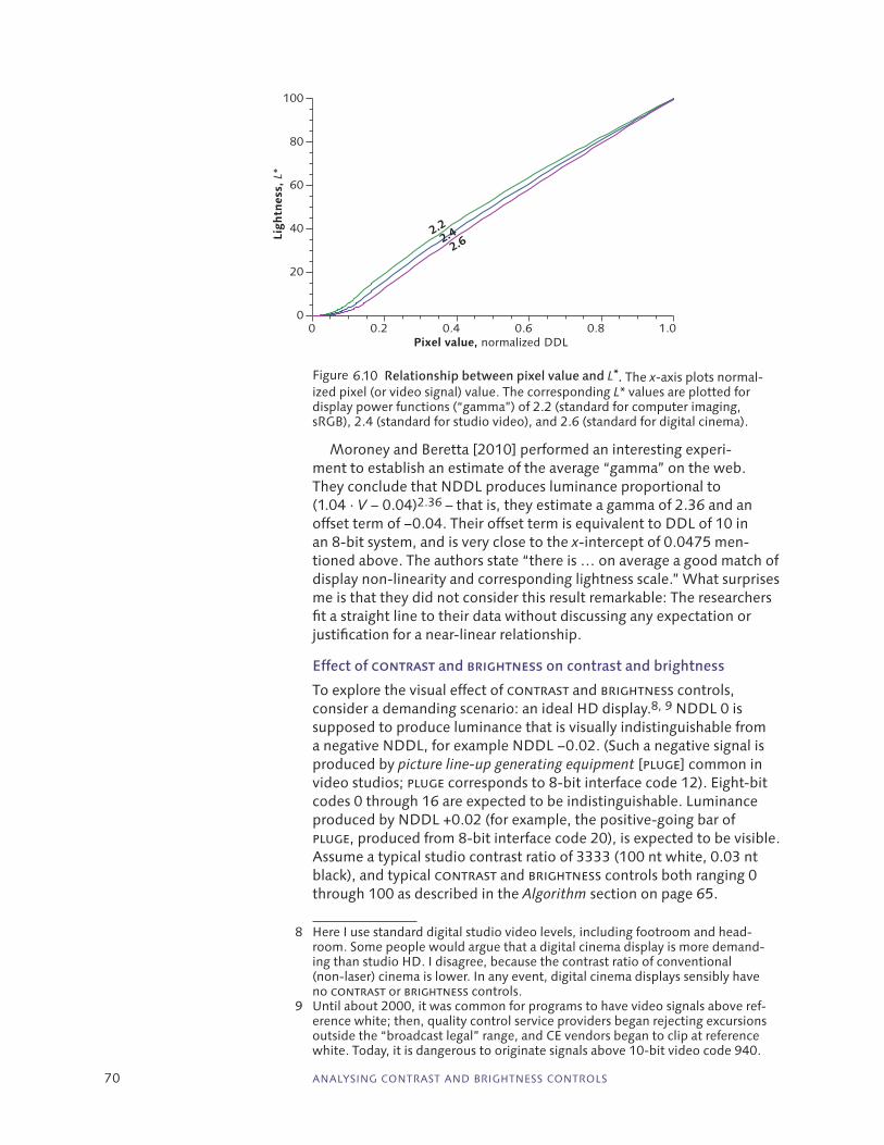
70 ANALYSING CONTRAST AND BRIGHTNESS CONTROLS
Moroney and Beretta [2010] performed an interesting experi-ment to establish an estimate of the average “gamma” on the web. They conclude that NDDL produces luminance proportional to (1.04 · V − 0.04)2.36 – that is, they estimate a gamma of 2.36 and an offset term of −0.04. Their offset term is equivalent to DDL of 10 in an 8-bit system, and is very close to the x-intercept of 0.0475 men-tioned above. The authors state “there is … on average a good match of display non-linearity and corresponding lightness scale.” What surprises me is that they did not consider this result remarkable: The researchers fit a straight line to their data without discussing any expectation or justification for a near-linear relationship.
Effect of contrast and brightness on contrast and brightness
To explore the visual effect of contrast and brightness controls, consider a demanding scenario: an ideal HD display.8, 9 NDDL 0 is supposed to produce luminance that is visually indistinguishable from a negative NDDL, for example NDDL −0.02. (Such a negative signal is produced by picture line‑up generating equipment [pluge] common in video studios; pluge corresponds to 8-bit interface code 12). Eight-bit codes 0 through 16 are expected to be indistinguishable. Luminance produced by NDDL +0.02 (for example, the positive-going bar of pluge, produced from 8-bit interface code 20), is expected to be visible. Assume a typical studio contrast ratio of 3333 (100 nt white, 0.03 nt black), and typical contrast and brightness controls both ranging 0 through 100 as described in the Algorithm section on page 65.
8 Here I use standard digital studio video levels, including footroom and head-room. Some people would argue that a digital cinema display is more demand-ing than studio HD. I disagree, because the contrast ratio of conventional (non-laser) cinema is lower. In any event, digital cinema displays sensibly have no contrast or brightness controls.
9 Until about 2000, it was common for programs to have video signals above ref-erence white; then, quality control service providers began rejecting excursions outside the “broadcast legal” range, and CE vendors began to clip at reference white. Today, it is dangerous to originate signals above 10-bit video code 940.
0.20 0.4 0.6 0.8 1.0
20
0
40
60
80
100
Pixel value, normalized DDL
Ligh
tnes
s, L
*
2.22.4
2.6
Figure 6.10 Relationship between pixel value and L* . The x-axis plots normal-ized pixel (or video signal) value. The corresponding L* values are plotted for display power functions (“gamma”) of 2.2 (standard for computer imaging, sRGB), 2.4 (standard for studio video), and 2.6 (standard for digital cinema).

CHAPTER 6 ANALYSING CONTRAST AND BRIGHTNESS CONTROLS 71
Decreasing brightness from its optimum setting causes clipping of any video content that lies barely above reference black. Clipping does not impair contrast ratio per se, but stripping out image content “in the shadows” produces obvious artifacts, so we will not explore decreasing brightness.
To compute the effect of contrast on contrast ratio, take the ratio of the luminance of white to the luminance of black:
CRm b
b=
+( )2 4
13333
2 4
.
.[ , ]maxEquation 6.3
Decreasing contrast from 50 to 30 reduces the white video signal to 0.8, yielding a relative luminance of 0.585. Increasing contrast from 50 to 70 increases the white signal to 1.25, yielding a relative luminance of 1.71. Starting with contrast ratio of 3333, adjusting contrast ±20 decreases contrast ratio to about 1950:1 or increases it to about 5700:1.
To compute the effect of contrast on “brightness,” estimate the user’s perception of display brightness by using L*:
L m b* [( ) ]. /= ⋅ + −116 162 4 1 3Equation 6.4
Adjusting contrast ±20 yields L* ranging from 81 to 118. To compute the effect of increasing brightness on contrast
ratio, increasing brightness from 50 to 70 takes the y-intercept of the 2.4-gamma curve of Figure 6.10 from −5 to +3. Reference black code now produces relative luminance of about 0.00332; reference white produces relative luminance of about 1.08. Increasing brightness thus causes contrast ratio to drop from 3333 to 1/0.00332 , that is, to 325.
Increasing brightness from 50 to 70 causes the reference white sig-nal to increase L* to 103.
To summarize contrast ratio, increasing contrast by 20 takes contrast ratio from 3333 to 5700, roughly a factor of 2. Increasing brightness by 20 drops contrast ratio from 3333 to 325, roughly a factor of 10. A 20-unit change in brightness has much more effect on contrast ratio than a 20-unit change in contrast.
To summarize display lightness, increasing brightness from 50 to 70 takes L* from 100 to 103, but increasing contrast from 50 to 70 takes L* from 100 to 118. Contrast has a much larger effect than brightness on the user’s perception of display brightness.
The results are summarized in this table:
Contrast ratio Ref. black L* Ref. white L*
Nominal 3333 0.3 100
Decrease contrast 20% 1950 0.5 81
Increase contrast 20% 5700 0.2 118
Increase brightness 20% 325 2.8 103
Table 6.1 Effect of adjusting contrast and brightness

72 ANALYSING CONTRAST AND BRIGHTNESS CONTROLS
This numerical example is elaborated by the four graphs of Fig-ure 6.11, which show the effect on contrast ratio (at the top) and lightness (L*, at the bottom) of adjusting contrast (at the left) and brightness (at the right), where the contrast and brightness scales correspond to the mappings to m and b of Equation 6.2. The optimiz-ation of contrast ratio by choosing the appropriate brightness setting is clearly evident in the peak of the top-right graph. The other three graphs show clipping, which for this example I have taken to set in at a video level of 125% of reference white, corresponding to relative luminance of 1.71.
From the right-hand halves of the two top graphs it is evident that an adjustment to brightness above its optimum setting causes con-trast ratio to decrease at roughly three times the rate that contrast ratio increases when contrast is adjusted (in its non-clipped region): Contrast ratio is more responsive to brightness than to contrast. From the bottom graphs, adjusting either contrast or brightness upwards increases the lightness of white (until the onset of clipping), but the typical contrast control is about three times more responsive.
LCDs
By the year 2000, display technology was shifting from CRTs to LCDs;
at the same time, digital driving circuitry was replacing analog. Today, the shift is complete. CRTs are obsolete, and digital driving circuits are ubiquitous.
It was a commercial requirement for the emerging technology to pro-duce the same response – from signal to light – as the entrenched CRTs. LCD displays do not have the same native physical response as CRTs, so display system developers incorporated into the signal processing a mapping that was the combination of two functions (but typically implemented in a single circuit or table lookup): the inverse of the dis-play’s native physical response, cascaded with a power function appro-priate for the CRT being replaced. In the case of an LCD, it’s complex, as the LCD native characteristic is roughly S-shaped.
LCDs are dramatically more stable than CRTs, and the need for adjustment to overcome drift was essentially eliminated. Nonetheless, contrast and brightness were carried forward into digital display tech-nology. In today’s equipment, these controls are implemented in the digital signal processing path in a digital version of the historical gain and offset processing.
Gain (contrast) can be implemented in the signal path, at the risk of introducing contouring artifacts. In an LCD, it is more sensible to modulate luminance through analog control of backlight power. For any display having a power-function EOTF – such as an sRGB display or a studio video display – backlight power level and traditional contrast setting are related by the display EOTF, according to this simple alge-braic identity:
Equation 6.5 ( )m x m x⋅ ≡ ⋅γ γ γ
The left-hand side of this equation represents gain adjustment in the signal path through traditional contrast; the right-hand side represents scaling the light output by modulating the backlight power. In theory, separate backlight and contrast controls are redundant.

CHAPTER 6 ANALYSING CONTRAST AND BRIGHTNESS CONTROLS 73
It is advantageous to implement traditional contrast through back-light modulation – in the optical analog domain – for two reasons. First, power is saved when backlight power is set less than maximum. Second, having contrast leave the video signal untouched main-tains the full digital signal range, and thereby avoids introduction of contouring.
It is pervasive that both professional and consumer display products have both backlight and contrast controls. In such cases, backlight should be used to control the display luminance, because moving contrast away from its detent is likely to introduce rounding or requantization errors in the signal path and thereby deteriorate image quality.
Some display products have controls labelled luminance; presum-ably such controls alter backlight power. If a display having a luminance control also has a contrast control, contrast should be set at detent and luminance should be used to control display luminance.
One display model has separate brightness, contrast, and black level adjustments, along with a user manual containing inscrut-able explanations [LaCie 2011]. Presumably brightness alters backlight power, and both contrast and black level are implemented in the
Figure 6.11 Contrast ratio and lightness (L*) are graphed in the upper and lower pairs, as a function of the m parameter ranging 0.5 to 2 (with the typical contrast setting 0 to 100) graphed at the left, and the b parameter ranging ±0.2 (with the typical brightness setting 0 to 100) graphed at the right. The display EOTF underlying these graphs clips at about 109% of the video signal, that is, at a relative luminance of about 1.09 2.4 or 1.22. The light grey vertical lines indicate the default m = 1, b = 0 (typically, contrast 50 and brightness 50).
0 20 40 60 80 100 0 20 40 60 80 100200
500
1000
2000
5000C
ontr
ast
rati
o (l
og s
cale
)
200
500
1000
2000
5000
0 20 40 60 80 100 0 20 40 60 80 1000
20
40
60
80
100
120
CONTRAST
Ligh
tnes
s, L
*
0
20
40
60
80
100
120
BRIGHTNESS
0.5 1 2.0
Gain, m (log scale)0 0.1 0.2-0.1-0.2
Bias, b
Clipping at black
Clipping at white
Clipping at white
Clipping at black

74 ANALYSING CONTRAST AND BRIGHTNESS CONTROLS
digital signal path. Ideally, users of such displays will set contrast and black level at detent, and use brightness to alter display luminance.
Another display model has separate brightness, picture, and backlight adjustments, along with a user manual having inscrutable explanations [Sony 2008]. Presumably backlight alters backlight power, and both picture and brightness are implemented in the digital signal path. Ideally, users of such displays will set brightness and picture at detent, and use backlight to alter display luminance.
Finally, another display model has separate backlight, contrast, and brightness adjustments, along with a user manual explaining that if backlight is increased, “The screen brightens,” and that brightness should be increased “For more brightness.” [Sharp 2012] Presumably backlight alters backlight power, and both contrast and brightness are implemented in the digital signal path. Like the previous example, users should leave brightness and picture at detent, and use backlight to alter display luminance.
As mentioned earlier, the typical contrast control range is equiva-lent to setting video gain between 0.5 and 2. For the 2.2-power of sRGB, a signal ratio of 2 yields a power (or luminance) ratio of 2 2.2, or about 4.6. It is highly unlikely that a display manufacturer will take a display having maximum luminance of 320 nt and establish a factory contrast setting correspond to 1/4.6 · 320, or 70 nt, in order to achieve perfect contrast control throughout the range of that control. One approach is to have factory setting of contrast at 100, corresponding to full backlight power; any contrast setting below 100 then simply reduces backlight power. However, some users in some situations wish to obtain higher average brightness, and are willing to compromise tone response, even potentially suffering some degree of highlight clip-ping. So the display manufacturer will be tempted to arrange maximum backlight power to be delivered at a factory setting of contrast lower than 100, and implement a two-stage contrast control where settings below the default reduce the backlight power (but preserve the video signal without clipping), and settings above the default produce max-imum backlight power and impose electrical gain in the signal path. The more gain, the more potential video signal clipping.
The behaviour of such a two-stage scheme is graphed in Figure 6.12. The relationship of gain factor and backlight power is shown in for the 2.2-power function of sRGB, for the contrast range 0 to 50 (that is, for gain from 0.5 to 1). For contrast between 50 and 100, gain between 1 and 2 is applied in the signal path. In the region where signal gain is applied, clipping will occur for some picture content; by the time gain of 2 is reached, video above level 0.5 will be clipped. Furthermore, any multiplication operation on signal component values is liable to impose requantization errors, depending upon the bit depths in pro-cessing and the bit depth at the display interface.
An alternate interpretation
In Figure 6.6 and Figure 6.7 (on page 66), several display curves were shown as a function of a fixed NDDL scale on the x-axis. In Figure 6.8 and Figure 6.9, the contrast and brightness controls were interpreted as changing the display’s response for a fixed scale of input values (normalized DDLs). Turn that around, and consider the display response

CHAPTER 6 ANALYSING CONTRAST AND BRIGHTNESS CONTROLS 75
to be a fixed function of display reference values ranging 0 through 1. Equation 6.1 implements a linear operation on the x-axis of Figure 6.10. Adjustment of contrast and brightness can therefore be interpreted as scaling and offsetting along the x-axis.
We can establish a parameter B (accessible to the user as black level) to control the display reference value intended to be produced by NDDL 0, and parameter W (accessible to the user as white level) to control the display reference value intended to be produced by NDDL 1.
Figure 6.13 shows the new interpretation. The x-axis in Figure 6.8 and Figure 6.9 has been relabelled Display reference value; under-neath that is the Pixel value (normalized DDL) scale. The NDDL scale is now squeezed or stretched, and offset. The example of Figure 6.9 has black level of +0.1, elevated from reference level so that NDDL 0 produces L* of about 3; white level of 0.9 causes NDDL 1 to produce L* of about 90.
The reparameterized version of Equation 6.1 is this:
Equation 6.6 y W B x B= −( ) ⋅ +
To implement an offset range comparable to a conventional brightness control, and to allow treatment of input signals that have black-level errors, settings for B should range about ±0.2. To be comparable to the gain range of a conventional contrast control,
Figure 6.12 Backlight power can be modulated to mimic the traditional contrast control. Providing both backlight and contrast controls is redundant. Traditional contrast setting can be mapped to a gain factor which is then mapped through the display’s EOTF (for example, the 2.2-power EOTF of sRGB, graphed here). Here, maximum backlight power is produced at default contrast setting, 50. Beyond that, signal path gain is applied; however, requantization is liable to degrade signal quality and clipping will occur for some signal content.
0
0.2
0
0.4
0.6
0.8
1.0
0.4 0.6 0.8 1.0
0
0.5
0
1.0
1.5
2.0
1.0 1.2 1.4 1.6 1.8 2.0
Gain factor, m
Gain factor, m
Traditional contrast setting
Bac
klig
ht o
ptic
al p
ower
(n
orm
aliz
ed)
Sign
al‑p
ath
gain
50 70300 100

76 ANALYSING CONTRAST AND BRIGHTNESS CONTROLS
settings for W should extend from 0.5 to 2.0. Most displays will be expected to exhibit clipping at W values greater than about 1.2, and it may be desirable to limit the user setting to such a value.
One advantage of this scheme is that black level and white level are more likely to be understood by the user than contrast and brightness. Another advantage is that there is no order dependence of operations: The user sees the controls as being independent, free from interaction.10
Black level setting
To set brightness (or black level) in studio video, display a pattern such as that standardized in ITU-R BT.814-2 containing pluge (levels −0.02, 0, +0.02) on a test image having average relative luminance of about 0.01 (1%). Set black level high, then reduce it until the −0.02 pluge level becomes visually indistinguishable from the 0 pluge level. That’s it: You’re done.
If you have no pluge pattern, display a picture that is predomin-antly or entirely black. Set black level to its minimum, then increase its level until the display barely shows a hint of dark grey, then back off a smidge.
Once black level is set correctly, contrast can be set to whatever level is appropriate for comfortable viewing, provided that clipping is avoided. In the studio, the contrast control can be used to achieve the
10 A different reparametrization, also exhibiting no control interaction, is the window level and window width (wl/ww) scheme that is common in med-ical imaging. See Window and level, on page 82.
Figure 6.13 Black level and white level controls . The display is viewed as having a fixed conversion from display reference values (0 to slightly more than 1) to luminance. Instead of contrast and brightness, black level and white level controls (indicated by the black and white triangles above) set the display reference values that correspond to NDDL values 0 and 1. In this example, black level is set to 0.1 and white level to 0.9. This example’s black level and white level settings of 0.1 and 0.9 cause the gain parameter m of Equation 6.1 to be computed as 0.8 and the bias (offset) parameter b as +0.1.
0.20 0.4 0.6 0.8 1.0
20
0
40
60
80
100
-0.2 1.2
0.20 0.4 0.6 0.8 1.0Pixel value, normalized DDL
Display reference value
Ligh
tnes
s, L
*

CHAPTER 6 ANALYSING CONTRAST AND BRIGHTNESS CONTROLS 77
desired luminance of reference white. Unfortunately, no current studio standard specifies the luminance of reference white; many studios11 choose 100 cd · m−2.
Historically, black level was sometimes adjusted to compensate drift of analog electronic components. Modern display equipment is very stable, and frequent adjustment is unnecessary. Historically, black level was sometimes used to compensate inaccuracies in source material; however, modern sources are quite reliable, and user adjust-ment to compensate poor sources is no longer required. Historically, black level setting was somewhat dependent upon ambient light. The diffuse ambient reflectance of modern displays is very low, around 0.01. This value is so low that ambient light contributes very little unwanted luminance, and has a minor effect on contrast ratio. Consumer adjust-ment in order to mitigate ambient light is no longer required.
For all of these reasons, manufacturers of consumer equipment should consider abolishing black level control (as Apple has done), or relegating it to an internal or service adjustment.
Historically, separate bias (or screen) calibration adjustments were provided for CRTs to allow a technician to null-out any difference in drift between channels that would otherwise cause a black input signal to display as a dark colour. Provision of such adjustments on LCDs and PDPs is insidious, because neither of these technologies involve any physical mechanism that could cause differential drift. These adjust-ments should therefore be abolished.
Non‑entertainment applications
Dr. Kristina Hellén-Halme and her colleagues reported research [2008a] concerning the analysis of dental radiographs (x-rays):
… the most accurate diagnosis of carious lesions was made when viewing the radiograph on a monitor that had been optimally adjusted …
She summarized that research for general dentists [2008b]:
… The accuracy of approximal caries diagnoses is higher when monitor brightness and contrast have been set at levels that are optimal for the task.
Rendering her conclusion in laymans’ terms, proper display settings affect health. But is she referring to brightness or brightness? Contrast or contrast? Clearly she is conscientious about display controls, but it’s unlikely that the majority of dentists understand contrast and brightness controls, nor should they be expected to.
Another medical display practitioner [Seto 2005] advocates leaving the display controls alone, and modifying images through application software:
… Disabling user control of the display settings and training the users to modify … the PACS viewer application instead of chang‑ing the monitor contrast and brightness will also help …
11 In the CRT era, studios in Europe used a somewhat lower reference white luminance, around 80 cd · m−2.

78 ANALYSING CONTRAST AND BRIGHTNESS CONTROLS
In a different professional domain, consider the following passages from a technical report of the U. S. Federal Aviation Administration [FAA 2007]. The technical report describes design criteria to be used in air traffic control displays:
5.1.6.9 Provide adjustable contrast and brightness. Controls shall be provided that are capable of providing multiple step or con‑tinuously variable contrast and brightness …
Does the FAA intend the terms “contrast” and “brightness” in this passage to refer to the perceptual phenomenon or to the like-named controls? The remainder of the document offers no hint. You might think that the interpretation of this passage is inconsequential; it merely indicates that two controls should be provided. But consider these two additional passages that are more specific about function:
5.1.6.10 Luminance range. A control should allow the user to vary the luminance from 10% luminance to 100% luminance. …
5.1.6.13 Contrast adjustment. A control shall be provided to ad‑just the foreground‑background contrast ratio.
To effect the change in luminance of the first passage, would a typical air traffic controller use the knob or slider labelled contrast or the one labelled brightness? The second passage has three instances of the word “contrast.” To effect that change of contrast, would a typical air traffic controller be expected to use the contrast control or the brightness control?
In my view, there is no reason to expect that professional users – including those people whose work concerns health and safety – should be knowledgeable about the engineering behind today’s display con-trols. Their job is in front of the display, not behind it. They deserve to have the display controls labelled in a manner directly related to their visual function. In my view, it is the display designers’ task to provide controls that are visually meaningful.
Summary
For the historical brightness and contrast controls of video, the dominant effect of changing contrast is to change brightness and the dominant effect of increasing brightness (from its optimum setting) is to reduce contrast ratio. In my view, this conclusion is not obvious. The roots of this relationship lie in analog CRT technology.
Burns [1959] and his colleagues at RCA wrote:
… the average viewer does not understand these controls well enough to clearly connect what is needed to what the controls do to be able to obtain an optimum picture except by a trial and error process.
More than half a century later the situation has not improved – in fact, owing to a much wider diversity of display types, a large degree of inconsistency in manufacturers’ implementations, confusion in control legends, and confusion in the information that is provided to both pro-fessional users and consumers, the situation is worse.

CHAPTER 6 ANALYSING CONTRAST AND BRIGHTNESS CONTROLS 79
In modern technology it is easy by design to present a black input signal as the darkest black possible. The situation for consumers and computer users – as well as for dentists, air traffic controllers, and other professionals – would be greatly improved if display manufacturers abolished user adjustment of bias, and thereby eliminated user-access-ible brightness controls.
Only a negligible fraction of users can be expected to understand display controls well enough to adjust black level to compensate ambi-ent light. For professional displays, it may be appropriate to provide a black level control, accomplishing the function formerly labelled brightness.
Contrast and brightness are confused by prior usage, so a new name is needed for user control of display lightness with respect to maximum available display luminance. I propose the name luminance for this control (whether calibrated or not).

80

81
7 Analysis of greyscale
medical image display
Perceptual uniformity was described in Chapter 3, on page 11. Peter Barten [1999, 2004] developed an analytical model of the luminance threshold of human vision over a wide range of luminance levels. The medical imaging community adapted and standardized Barten’s model to greyscale imaging; the standard is now widely used. Appli-cation-specific image data values are placed on a uniform perceptual scale bounded by the minimum and maximum luminance that can be produced by a particular display. There is a subtle interplay between the approximate perceptual uniformity provided by the default sRGB behaviour of typical displays (including medical displays) and the explicit perceptual uniformity implemented by the dicom GSDF. This chapter analyses the dicom image display process, emphasizing the calibration model and the perceptual nature of the mapping.
DICOM
Digital Imaging and Communications in Medicine (dicom) refers to a set of standards promulgated by National Electrical Manufacturers Asso-ciation (nema), in association with the American College of Radiology (acr). The standard concerns processing, distributing, and viewing digital medical images. The standard document PS 3.14 (“Part 14”) relates to the calibration and display of greyscale images [ACR/NEMA 2009]. Figure 7.1 illustrates the conceptual processing chain.
Figure 7.1 Dicom block diagram is adapted from Figures 6.1 and 6.2 of the standard. The “Standardized Display System” is illustrated in the dicom standard as a block; however, digital drive levels (DDLs) are conveyed from a computer graphics subsystem across an interface (such as DVI) to a display device, so the line labelled DDLs is the typically external interface to the display. Conversion of P ‑values to DDLs is typically implemented by a LUT loaded into the computer’s graphics subsystem.
Image data(Modality-specific)
Values ofinterest, Polarity
Image presentation
Specialized PC Hardware/Software
Standardized Display System
Lumina
nce
P-Valu
es
DDLs
window and level
Display
driv
er
& LCD
pan
elj(eocf-1(L))
Display unit
Calibration

82 ANALYSIS OF GREYSCALE MEDICAL IMAGE DISPLAY
The dicom model starts with image data values dependent upon imaging modality – that is, upon the type of equipment used to produce the imagery. For example, in computed tomography (CT), Hounsfield units (HU) ranging −1000 … +3000 are used; by defin-ition, air has attenuation −1000 HU and water has attenuation 0 HU [Hounsfield 1980; Jackson 2004]. In other modalities, data in ranges such as 0 … 255, 0 … 1023, or 0 … 4095 may be used. Application software provides a default mapping to the display luminance range. For example, to encode Hounsfield Units into 10-bit integer pixel values, data values ±1000 are typically offset by +1000 then scaled by 1023/2000.
Through the mechanism described in the remainder of this chapter, data values are displayed in a perceptually uniform manner. Medical practitioners commonly refer to perceptual linearization, or perceptually linear values [Samei 2005]; however, it seems to me that linear is too strong a term to be applied to a perceptual process that no instrument can directly measure. The term perceptual uniformity is used here (see Chapter 3, Perceptual uniformity in digital imaging, on page 11).
Window and level
In some medical imaging modalities, useful data may occupy a few thousand levels (such as the 4000 levels of CT data when expressed in Hounsfield units); however, human vision cannot discern 4000 shades of grey at one glance. In medical application software, window width (ww) and window level (wl) adjustments1 [Hsieh 2009; Pooley 2001] are typically provided to allow the viewer – for example, a radiolo-gist – to amplify differences in a certain range of image data values. The controls are commonly called window and level. Window serves as a wide-range gain control; it sets the fraction of the input data range that is to be mapped into the full output signal range. Level serves as a wide-range offset control: Level is set by the viewer to the data value that is to produce output of y = 0.5, halfway up the result perceptual scale. Clipping is routinely expected.
Window and level are typically expressed in a modality-specific manner, either in terms of data values standard for the modality (e.g., Hounsfield units for computed tomography, CT), or in terms of integer pixel values. In the default mapping, the window encompasses the entire data range, and the halfway point in that range is mapped to an output of 0.5. In an application that presents 12 bit values 0 through 4095, ww and wl both range 0 to 4095, and the “unity” mapping is ww = 4096, wl = 2048. In this 12-bit coding, setting ww to 1024 has the effect amplifying by 4, which causes 1/4 of the input range to span the full output range (and causes 3/4 of the input range to be lost to clipping). For data value D, ww value, and wl value all normalized to the same range, windowing returns a result P potentially from 0 through 1023 according to this transfer function:
P D= ⋅ + ⋅ −
10231
0 112
Clipww
wl( ), ,{ }Equation 7.1
1 Window width and window level adjustments are apparently so common-place in medical imaging that it’s difficult to find a definitive reference to their operation.

CHAPTER 7 ANALYSIS OF GREYSCALE MEDICAL IMAGE DISPLAY 83
Clipping is defined to return a result which is the argument, unless it lies outside specified minimum and maximum values:
Clip x L HH H xx L x HL x L
, ,,,,
{ }( )<< ≤≤
=Equation 7.2
Medical imaging equipment is typically equipped with a set of select-able, predefined window/level settings. For example, a CT scanner typically has a default “bone window” and a default “soft tissue win-dow”; these are optimized for visual examination of the respective structures.
Medical displays are typically well calibrated, so medical practi-tioners don’t need controls to compensate the displays. The contrast and brightness controls found on commodity displays aren’t typically found in medical displays. Window and level are not used to calibrate displays; they are used to aid in examining the image data.
Following value-of-interest (window/level) processing, data is optionally inverted in the Polarity block of Figure 7.1. (Inversion is math-ematically equivalent to negating the ww parameter in Equation 7.1). The result is a presentation value (P‑value), crossing the vertical line in Figure 7.1 that separates dicom from Image Presentation. P-values lie in the range 0 through 1023.
P-values are mapped to jnd index values ( j values), thence to digital drive levels (DDLs) presented to the display unit, through a mapping that we will describe. The mapping depends upon the dicom GSDF and upon the characteristics of the display to be used.
DICOM GSDF
The dicom greyscale display function (GSDF) is a standardized nonlinear function L( j) that transforms a jnd index value2 denoted j, ranging 1 through 1023, to an absolute luminance from L(1) of 0.05 cd · m−2 to L(1023) of 4000 cd · m−2. The function L( j ) is based upon the ratio of two polynomials in ln ( j ); the quotient provides the log10 of abso-lute luminance. The numerator is a fourth degree polynomial, and the denominator is fifth degree; the coefficients are expressed to six digits:3
L( )
. . ln( ) .
j
j
=
− + ⋅ + ⋅
10
1 0 08 0 13011877 0242636 3646699 lln( ) . ln( ) . ln( )j j j2 3 40 02 0 001
1
5468404 3635334− ⋅ + ⋅
−− ⋅ − ⋅ +0 02 0 1 0 025840191 0320229 874562. ln( ) . ln( ) .j j 220 1978977 29926340 003 0 00013 4⋅ − ⋅ + ⋅ln( ) . ln( ) . lnj j (( )j 5
Equation 7.3
The function is graphed in Figure 7.2; the y-axis is plotted on a log scale, so the curve as presented in that graph is the rational polynomial enclosed in parentheses in Equation 7.3.
Clearly, zero must not be presented as an argument to the function defined in Equation 7.3. The calibration process to be described below returns j-values strictly in the range 1 through 1023, and zero never appears in a proper mapping from P-values.
2 The dicom group determined that about 1000 JND increments lie between 0.05 cd · m−2 and 4000 cd · m − 2. The choice of 1023 JND indices sug-gests an optimization for 10-bit coding; however, for practical displays P-values are mapped to a subset of the complete j range. Why 1023 codes are used instead of 1000 is not apparent.
3 Equation 7.3 and Equation 7.4 are included here for illustrative purposes only. Implementors are advised to consult the standard.

84 ANALYSIS OF GREYSCALE MEDICAL IMAGE DISPLAY
P-values that are presented to the GSDF are implicitly perceptually uniform. In the case of Hounsfield units for CT, the data represents a computed linear attenuation coefficient that acts as an exponent. Each pixel value is proportional to the logarithm of X-ray radiance after traversing the path to that pixel. CT image data therefore has the char-acter of a logarithmic encoding:
The inverse mapping, from absolute luminance L to jnd index value j, is defined by this eighth-degree polynomial in log10(L) having nine, eight-digit coefficients:
j( ) . . log ( ) . logL L= + ⋅ + ⋅71 498068 94 593053 41 91205310 1102
103
109 8247004 0 28175407( ) . log ( ) . log ( )L L L+ ⋅ + ⋅ 44
105
1061 1878455 0 18014349 0 1− ⋅ − ⋅ +. log ( ) . log ( ) .L L 44710899 0 01704684510
710
8⋅ − ⋅log ( ) . log ( )L L
Equation 7.4
The GSDF luminance extremes are well beyond what is available in electronic displays today, and the contrast ratio of 80 000:1 (about 4.9 log10 units) between the extremes is well beyond what is available in electronic displays today. Medical image data values are mapped into a practical range through the technique to be described below.
The perceptual uniformity of the L( j ) mapping can be characterized by Weber contrast, that is, the ratio of absolute luminance values asso-ciated with two adjacent jnd index values. The Weber contrast between the lowest pair of j values – that is, the ratio L(2)/L(1) – is about 1.09. At j value 268, the Weber contrast has fallen to 1.01; for j exceed-ing 269, Weber contrast gradually falls to the ratio L(1023)/L(1022) , about 1.006, shown in Figure 7.3. Across the top octave of luminance, from 2000 cd · m−2 to 4000 cd · m−2 – that is, across one log2 unit, or one photographic stop – there are 106 j values.
Figure 7.2 Dicom grayscale display function L( j ) maps jnd index j (from 1 through 1023) to absolute luminance (here graphed on a log scale).
0 200 400 600 800 1000
0.10.05
1
10
100
1000
4000
JND index, j
Lum
inan
ce, L
(j)
[nt]
(lo
g sc
ale)
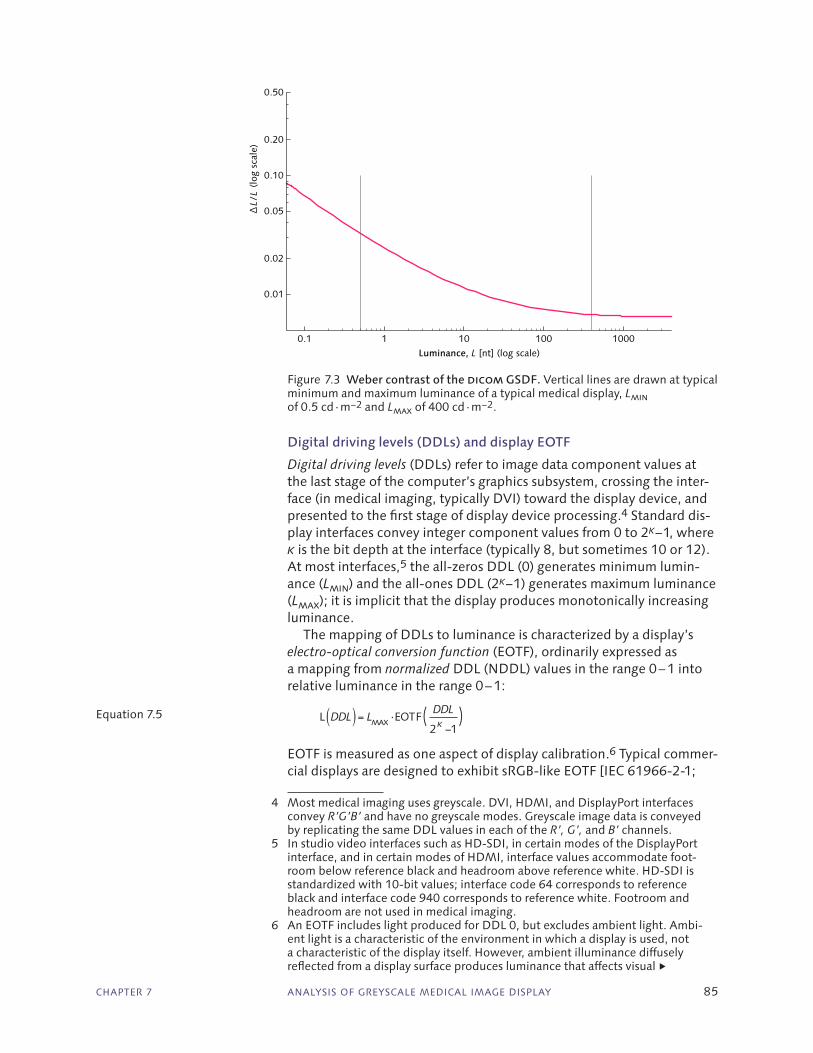
CHAPTER 7 ANALYSIS OF GREYSCALE MEDICAL IMAGE DISPLAY 85
Digital driving levels (DDLs) and display EOTF
Digital driving levels (DDLs) refer to image data component values at the last stage of the computer’s graphics subsystem, crossing the inter-face (in medical imaging, typically DVI) toward the display device, and presented to the first stage of display device processing.4 Standard dis-play interfaces convey integer component values from 0 to 2k−1, where k is the bit depth at the interface (typically 8, but sometimes 10 or 12). At most interfaces,5 the all-zeros DDL (0) generates minimum lumin-ance (Lmin) and the all-ones DDL (2k−1) generates maximum luminance (Lmax); it is implicit that the display produces monotonically increasing luminance.
The mapping of DDLs to luminance is characterized by a display’s electro‑optical conversion function (EOTF), ordinarily expressed as a mapping from normalized DDL (NDDL) values in the range 0 – 1 into relative luminance in the range 0 – 1:
L EOT· F( )DDL LDDLk( ) =−
max2 1
Equation 7.5
EOTF is measured as one aspect of display calibration.6 Typical commer-cial displays are designed to exhibit sRGB-like EOTF [IEC 61966-2-1;
4 Most medical imaging uses greyscale. DVI, HDMI, and DisplayPort interfaces convey R’G’B’ and have no greyscale modes. Greyscale image data is conveyed by replicating the same DDL values in each of the R’, G’, and B’ channels.
5 In studio video interfaces such as HD-SDI, in certain modes of the DisplayPort interface, and in certain modes of HDMI, interface values accommodate foot-room below reference black and headroom above reference white. HD-SDI is standardized with 10-bit values; interface code 64 corresponds to reference black and interface code 940 corresponds to reference white. Footroom and headroom are not used in medical imaging.
6 An EOTF includes light produced for DDL 0, but excludes ambient light. Ambi-ent light is a characteristic of the environment in which a display is used, not a characteristic of the display itself. However, ambient illuminance diffusely reflected from a display surface produces luminance that affects visual ▶
0.1 1 10 100 1000
0.01
0.02
0.05
0.10
0.20
0.50
Luminance, L [nt] (log scale)
∆L/
L (lo
g sc
ale)
Figure 7.3 Weber contrast of the dicom GSDF . Vertical lines are drawn at typical minimum and maximum luminance of a typical medical display, Lmin of 0.5 cd · m−2 and Lmax of 400 cd · m−2.

86 ANALYSIS OF GREYSCALE MEDICAL IMAGE DISPLAY
Stokes 1996]: The mapping from DDL to relative luminance resembles a 2.2 power function. Typical LCD panels have intrinsic native response that is somewhat S-shaped [Lee 2005]; a typical LCD display unit incor-porates an internal circuitry (sometimes including a lookup table) that maps DDLs into panel driving levels that are presented to the digit-al-to-analog converters. The DACs are typically incorporated into the column-driver circuits attached to the panel.
The sRGB specification calls for reference white luminance7 of 80 cd · m−2; however, that aspect of the sRGB specification is outdated, and today’s displays typically have maximum luminance between 250 cd · m−2 and 400 cd · m−2. The sRGB specification calls for reference veiling glare of 0.2 cd · m−2; reference contrast ratio at the standard’s 80 cd · m−2 is thus 400:1, and modern displays now com-monly exhibit higher contrast ratio than 400:1.
As explained in Chapter 3, the 2.2 power of sRGB is remarkably per-ceptually uniform. The dicom display model would break down if the display’s EOTF were to depart significantly from perceptual uniformity; however, dicom places no specific requirement upon the display.
DICOM calibration
Conceptually, dicom image presentation takes P-values (ranging 0 to 1023, inclusive), and scales and offsets them into the range of j val-ues that lies between the luminance limits (Lmin and Lmax) of a particu-lar display:
j LP
L L= ( )+ ( ) − ( )( )j j jmin max min1023Equation 7.6
j values are then mapped through that portion of the GSDF L( j) func-tion that lies between the particular display’s minimum and maximum absolute luminance values (Lmin , produced by DDL value 0, and Lmax , produced by DDL 2 k−1) to produce the required absolute luminance. The DDL required to produce a particular absolute luminance is deter-mined by the inverse of measurements of the display’s mapping from DDL to luminance – that is, by mapping through EOTF−1.
In practice, the data mapping and the calibration in dicom are combined, and effected in a lookup table (LUT) loaded into the back-end of the graphics subsystem that drives the display – that is, the LUT is loaded into the block labelled P‑values to DDLs in Figure 7.1. Appli-cation P-values (following window and level processing and polarity control) are mapped through the LUT, whose contents are typically established to calibrate a specific display type or to calibrate a particular display unit [AAPM 2005; Fetterly 2008]. The operation of the LUT is simply this (where square brackets indicate table lookup):
DDL LUTP P( ) = Equation 7.7
▶ performance. dicom standards do not account for ambient light; however, guidelines have been established by the medical profession [Chawla 2007].
7 The sRGB standard has no footroom or headroom; the “reference” luminance of sRGB is comparable to a video engineer’s peak luminance.

CHAPTER 7 ANALYSIS OF GREYSCALE MEDICAL IMAGE DISPLAY 87
The LUT entries are constructed to map the full range of P-values (0 through 1023) into the full range of DDLs (0 through 2k−1, where k is the bit depth at the interface, typically 8).
The calibration LUT is constructed across all possible P-values 0 through 1023 by first mapping P to a j value using Equation 7.6, then mapping through the applicable portion of the dicom GSDF L( j) to obtain an absolute luminance, then mapping through the inverse of the display’s EOTF to obtain a DDL. In equation form, using Iverson’s “floor” notation:
LUT EOTF
j j
i
L Li
Lk⎡⎣ ⎤⎦ = + ( ) ⋅
( ) + (−
−12
1 121023min max )) − ( )⎡
⎣⎤⎦
⎛
⎝⎜
⎞
⎠⎟⎞
⎠
⎟⎟⎟
⎢
⎣
⎢⎢⎢⎢
⎥
⎦
⎥⎥⎥⎥
j L
L
min
maxEquation 7.8
At first glance, it appears that the dicom standard anticipates j val-ues that are 10 bit integers, excluding zero. Zero is, indeed, excluded; however, j values are not necessarily integers: In principle, calibration could implement arbitrary precision in the calculation of L( j), and could retain arbitrary precision in the device measurements that represent the inverse of the display’s mapping of DDL to luminance.
Summary
In the dicom image display model, application image data values are scaled and offset according to window width and window level controls, and a “polarity” (inversion) control, adjusted by the specialist viewer. These adjustments can be considered to be a reparametrization of video contrast and brightness controls.
Image signal values after window and level processing, P-values, are then mapped through a calibration LUT loaded into the graphics sub-system of the computer, producing DDLs that are conveyed across the interface to the display unit. For full-range window and level settings, any particular display produces absolute luminance values across the range of luminance levels produced by that display. The calibration LUT is built such that displayed luminance values lie along that portion of the dicom GSDF representing luminance values available on that par-ticular display.
The effect is that application P-values are presented on a uniform perceptual scale disposed across calibrated luminance levels across the minimum-to-maximum luminance range available for any particular dis-play unit. This concept of adaptation of image data values to a particu-lar display could be usefull applied to video display, and in particular, to HDR. However, the dicom model does not incorporate compensation of adaptation effects at viewing.

88

89
8 Wide colour gamut and high dynamic range
in HD and UHD1
Twenty four years ago, I presented and published a conference paper entitled “Wide gamut device-independent colour image interchange” [Poynton 1994]. The CCIR (now, ITU-R) Rec. 709 standard had just been adopted (in 1990), and, by 1994, sRGB deployment in desktop computing was well underway. That paper anticipated commercial interest in exchange of wide-gamut imagery. As it turned out, wide gamut was not imminent: We’ve had 25 years of very stable colour encoding for video in the form of BT.709 for HD (augmented in 2011 by BT.1886, which finally standardized the HD EOTF and enabled the emergence of mastering-display-referred video), and the BT.709-deriv-ative sRGB that remains ubiquitous in the computer domain.
Now, however, dramatic changes are underway. Wide colour gamut (WCG), enabled mainly by RGB LED backlights for LCD displays, has been deployed in consumer television. High dynamic range (HDR) cameras are commercially available; and HDR displays, mainly enabled by spatially modulated LED backlights, have been commercialized. Many industry experts agree that consumers experience WCG and HDR as more significant than increasing spatial resolution from HD (“2 k”) to “4 k”.
This chapter describes work performed jointly with Jeroen Stessen, Rutger Nijland, and their colleagues at Philips Research in Eindhoven. We revisit the topic of the 1994 paper, but now with some urgency, to address the question: How should wide colour gamut and high dynamic range video imagery be encoded? We conclude that the Y′CBCR tech-nique and its variants are perfectly adequate for moderate dynamic range but yield poor performance when combined with HDR. New encoding techniques are needed. We conclude that a perceptual quan-tizer (PQ) should replace the conventional gamma function to enable HDR. Chroma subsampling of CBCR components performs poorly in combination with the PQ; we propose encoding and decoding modified u′v′ chromaticity components instead of CBCR.
1 This chapter reports on joint work undertaken with Jeroen Stessen and Rutger Nijland, both of Philips Research, Eindhoven, Netherlands. This chapter is an edited version of a paper published in SMPTE Motion Imaging Journal [Poynton et al. 2015]. The authors earned a SMPTE 2015 Award of Merit.

90 WIDE COLOUR GAMUT AND HIGH DYNAMIC RANGE IN HD AND UHD
Introduction
For twenty years HD material has been mastered to a fixed set of display primaries, those standardized in ITU-R Rec. BT.1886, which are best described as having moderate colour gamut. The BT.1886 primaries were originally chosen in 1990 (as “Rec. 709”) to closely approximate the CRT phosphors that had been in use since about 1965. LCD dis-plays commercialized since 1995 have been designed to have primar-ies comparable to those of BT.1886, partly because virtually all of the available content was mastered to those primaries, and partly because BT.1886 primaries were easily achieved by CCFL and white LED back-light units (BLUs). Now, though, BLUs incorporating red, green, and blue LEDs are economical. Each of the red, green, and blue LED types has a rather narrow spectral spread (between about 25 nm and 35 nm); the narrow spectral coverage leads to the possibility of gamut wider than BT.1886. Typical RGB LED BLU technology enables display gamut approximately matching the P3 gamut of digital cinema. The possibility arises for studios to deliver movie-class colour gamut to consumers; movies would benefit, and so would sports and live events.
Consumers seem to like colourful pictures. Consumer electronics (CE) manufacturers have found that television sets producing colour-ful pictures are more profitable than those delivering pictures that are not colourful. Today, however, there is no wide colour gamut program material available. So, consumer manufacturers have built signal pro-cessing circuitry to expand the colour range of BT.1886 material. The colours that are displayed are not faithful to the original. One goal of our work is to allow content creation with wide gamut and to encode and decode in a way that it makes it possible to display authentic wide gamut colour to consumers.
The second development is high dynamic range, HDR [Daly 2013]. Conventional HD is approved at a contrast ratio of about 1000:1; dif-fuse white is portrayed at about 100 nt; and the blackest black is about 0.1 nt. Consumers prefer brighter pictures than those displayed at pro-gram creation: Today’s consumer experiences diffuse white at between 300 and 500 nt; black level is typically between 0.3 and 2 nt. For this contrast range, at consumer quality level, eight-bit components coded using a 2.4-power function, as defined in BT.1886, are sufficient. Ten-bit components are used in the studio, and ten bit components would deliver somewhat better performance to consumers than today’s eight bit components.
Much work has been done in HDR acquisition, and capture of live action at HDR is now fairly simple using several different camera types.
On the display side, a Canadian company called Brightside developed a particularly interesting type of display technology [Seetzen 2004]. Dolby acquired Brightside in 2007; Dolby has commer-cialized the technology in the consumer domain. The display involves an area array backlight comprising around a thousand LED clusters (instead of the more common linear array with a few dozen LED clus-ters); backlights are individually controlled, achieving spatial backlight modulation. Some CE manufacturers conceptualize the scheme starting with fully-on backlights and call the scheme “local dimming.” We prefer to say, “local brightening.” Should AMOLED displays be commercial-

CHAPTER 8 WIDE COLOUR GAMUT AND HIGH DYNAMIC RANGE IN HD AND UHD 91
ized for consumer television, we expect at least some of them also to be able deliver HDR-class imagery.
Our goal is to take WCG/HDR material at the approval stage of pro-duction (prior to mastering), and encode into signals that can be pre-sented to a conventional H.264/265 compressor. After decompression at the consumers’ premises, we decode for WCG/HDR display. We seek unlimited colour gamut, but we expect HDR displays to have gamut approximating that of the DCI P3 standard. Luminance of the portrayal of diffuse white need not be higher than about 500 nt, but we seek to portray specular highlights and directly light sources using luminance levels perhaps ten times higher than diffuse white, a capability unavail-able in today’s systems. We also seek to enable HDR displays to present blacks darker than today’s 0.3 nt or so.
Concepts
We will speak of an encoding standard. Historically, we would have said transmission standard, but that term fails to encompass modern distri-bution technologies. Decoding is as close as possible to the inverse of encoding; however, encoding is somewhat lossy, so encoding is not per-fectly inverted. We are not encoding the scene; we encode the material that is presented for approval at the final stage of post-production, immediately prior to mastering. By encoding and decoding, we refer to representing tone (greyscale) and colour.2 Here, wide gamut and HDR image data is encoded into to three components that are presented to such a compressor. After distribution, and decompression, the three colour components are decoded prior to display; see Poynton [2012].
When R′G′B′ signals are conveyed (or decoded from Y′CBCR), they are conveyed in display-referred form: The decoded XYZ components represent the colours intended to be displayed. CRT displays historic-ally had physical primaries matching the reference primaries defined in the encoding colour space, and also has an intrinsic EOTF matching the encoding standard.
In professional imaging, and especially entertainment imaging, encoding typically has only an indirect connection to the scene and the camera. In computer animation, or other synthetically generated content, there is no physical scene and no physical camera at all! In the general case, what is important to content creators is that the image displayed to the consumer is a reasonable approximation of the image as displayed on an approval display (e.g., studio reference display) at the end of the production and post-production chain.
Upstream of approval, there may be science, but what really matters is art and craft. Downstream of approval, ideally there is just science.
Today’s world offers a wide diversity of display devices; these display devices have a diversity of tone and colour characteristics. We expect a transform to take place at the viewing device to adapt transmission encoding to the native device. (For example, in today’s LCDs, the LCD driver circuitry incorporates compensation of the native LCD S-shaped EOTF function.) Today’s BT.1886 is not capable of HDR; in order to accommodate HDR content in the transmission chain, we’ll need an
2 The terms encoding and decoding are ambiguous because these terms are also used to refer to motion-compensated transform-based compression systems such as H.264/265.
92 WIDE COLOUR GAMUT AND HIGH DYNAMIC RANGE IN HD AND UHD
HDR-capable quantizer. A perceptual quantizer (PQ) was proposed by Dolby [Miller 2013] and has been standardized [SMPTE ST 2084].
The diversity of display devices comes with a diversity of physical dis-play primaries. Signal processing to accomplish a colour transform from the encoding (“transmission” or “interchange”) primaries to the display device is expected to be implemented at the viewing device. Many television engineers are familiar with colorimetric transforms imple-mented as 3 × 3 “linear-light” matrix processing to transform from one primary set to another. These transforms are perfectly suitable when the source colour space is completely contained within the destination space, as is the case in transforming BT.1886 to wide-gamut primaries such as those of DCI P3 or BT.2020. However, a nontrivial colorimetric transform never fills the destination colour space; CE manufacturers typically implement noncolorimetric transforms that stretch colours into the destination gamut in order to make pictures more colourful. When transforming to a destination space that has a smaller gamut than the source, a colorimetric transform is bound to clip some colours. We expect that colorimetric transforms will not suffice; we hope that some standards concerning gamut mapping can be established.
Historical video systems have used pure power functions at the dis-play. Y′CBCR interchange signals are converted to R′G′B′ image signals, and each of the R′G′B′ image signals is raised to approximately the 2.4-power to yield the display tristimulus RGB. The scheme is better than using code values proportional to light intensity (“linear-light”); however, power function coding places many more digital codes in the light tones than are needed, and not enough codes in the deep blacks. The way to optimize the coding for visual perception is to determine how many “just noticeable difference” ( jnd) steps are perceived by human vision and to quantize accordingly. Peter Barten, of Philips, com-pleted a very detailed study of this issue [Barten 1993, 1999]. We use Barten’s work to establish perceptual quantization (PQ).
Conventional video systems form a “luma” component representa-tive of the achromatic content of the image and two components carry-ing the “chroma”: Y′CBCR . The chroma components are subsampled, that is, spatially lowpass filtered (“downsampled”) typically in the 4:2:0 scheme where chroma resolution is reduced by a factor of 2:1 in both the horizontal and vertical domains. These calculations are done in the gamma-corrected domain (nonconstant luminance); so, the calculations are affected by the choice of R′G′B′ coding (gamma). The scheme works well for moderate R′G′B′ nonlinearity such as the 2.4-power function of the BT.1886 EOTF for HD. However, we have found that serious chroma subsampling artefacts result when the same calculation is performed on R′G′B′ signals having an HDR perceptual quantizer.
We propose to convey colour using true colour science chromaticity coordinates (u′, v′) instead of CBCR . We have found that (u′, v′) can be subsampled 4:2:0 without visible impairment. The system we propose has true constant luminance, owing to the fact that one compon-ent contains all of the CIE luminance. (An alternate scheme, ICTCP , approaches but does not achieve exact constant luminance. See the PhD thesis of Fröhlich [2017].)
The suggestion of using of (u′, v′) components for colour digital image data dates back many decades [Solomon 1975], prior to the
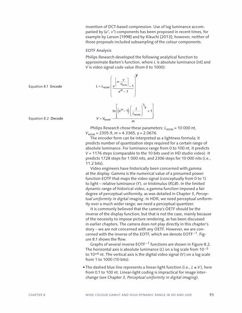
CHAPTER 8 WIDE COLOUR GAMUT AND HIGH DYNAMIC RANGE IN HD AND UHD 93
invention of DCT-based compression. Use of log luminance accom-panied by (u′, v′) components has been proposed in recent times, for example by Larson [1998] and by Kikuchi [2013]; however, neither of those proposals included subsampling of the colour components.
EOTF Analysis
Philips Research developed the following analytical function to approximate Barten’s function, where L is absolute luminance [nt] and V is video signal code value (from 0 to 1000):
Equation 8.1 Encode
L = Lnom· em·VVnom 1
em 1
γ
Equation 8.2 Decode
V = Vnom·
ln em 1( )· LLnom
1/
+ 1
m
γ
Philips Research chose these parameters: Lnom = 10 000 nt, Vnom = 2305.9, m = 4.3365, γ = 2.0676.
The encoder form can be interpreted as a lightness formula; it predicts number of quantization steps required for a certain range of absolute luminance. For luminance range from 0 to 100 nt, it predicts V = 1176 steps (comparable to the 10 bits used in HD studio video). It predicts 1728 steps for 1 000 nits, and 2306 steps for 10 000 nits (i.e., 11.2 bits).
Video engineers have historically been concerned with gamma at the display. Gamma is the numerical value of a presumed power function EOTF that maps the video signal (conceptually from 0 to 1) to light – relative luminance (Y ), or tristimulus (RGB). In the limited dynamic range of historical video, a gamma function imposed a fair degree of perceptual uniformity, as was detailed in Chapter 3, Percep‑tual uniformity in digital imaging. In HDR, we need perceptual uniform-ity over a much wider range; we need a perceptual quantizer.
It is commonly believed that the camera’s OETF should be the inverse of the display function; but that is not the case, mainly because of the necessity to impose picture rendering, as has been discussed in earlier chapters. The camera does not play directly in this chapter’s story – we are not concerned with any OETF. However, we are con-cerned with the inverse of the EOTF, which we denote EOTF −1. Fig-ure 8.1 shows the flow.
Graphs of several inverse EOTF −1 functions are shown in Figure 8.2. The horizontal axis is absolute luminance (L) on a log scale from 10 −3 to 10+4 nt. The vertical axis is the digital video signal (V ) on a log scale from 1 to 1000 (10 bits):
• The dashed blue line represents a linear-light function (i.e., L ∝ V ), here from 0.1 to 100 nt. Linear-light coding is impractical for image inter-change (see Chapter 3, Perceptual uniformity in digital imaging).

94 WIDE COLOUR GAMUT AND HIGH DYNAMIC RANGE IN HD AND UHD
• The dash-dot magenta line represents video decoding according to the BT.1886 standard; here, reference white is 100 nt. The line has a con-stant slope of 1/2.4.
• The solid magenta line represents a typical consumer television receiver EOTF from 0 to 500 nt. This line represents typical consumer TV receiver behaviour; the line has a constant slope of 1/2.2 , suitable for reference white luminance considerably higher than 100 nt and sur-round condition brighter than the mastering (approval) condition.
• The solid green line represents an HDR function from 0 to 5000 nt, pro-posed by Philips, inspired by Barten’s CSF, and similar to ST 2084 PQ. The dark part of this line has a slope of 1/2.35 . The bright part of the line is a logarithmic function. The logarithmic property allows an efficient expansion of the dynamic range to very high luminance, more so than any realistic power function.
A linear-light relative luminance signal is symbolized Y, in the gamma domain the signal is called luma and symbolized Y′. We will double-prime the corresponding quantities in the perceptually quantized domain: We will write Y” (and R″, G″, B″).
We can evaluate the visibility of quantization of the V signal for various functions. We plot Δ f/L against L, on log-log axes, for various functions f. The graph is presented in Figure 8.3.
In addition to the four EOTFs of the previous figure, the reciprocal of Barten’s CSF is added as a dashed red line; this line represents the just noticeable quantization step across the luminance range. Anything above the red dashed line is liable to be visible as a false contour. The linear-light signal is quantized far too coarsely at the dark end and far too finely at the bright end. The Barten CSF line shows that the dynamic range can be extended indefinitely at a ratio of 0.004, analogous to the Weber-Fechner “law.”
Approval displayStud
io co
de/
displa
y int
erfac
e
Cons
umer
code
/
displa
y int
erfac
e
Chan
nel
Camera
code
(e.g.,
log)
Consumerdisplay
CameraOETF
PQ PQ-1EOTF
modelEOTF
-1
model
DisplayEOTF(intrinsic)
Post/DI process
DisplayEOTF(intrinsic)
Figure 8.1 Simplified pipeline of an imaging system using the PQ EOTF is sketched.

CHAPTER 8 WIDE COLOUR GAMUT AND HIGH DYNAMIC RANGE IN HD AND UHD 95
Chroma versus Chromaticity
It is standard for (CB , CR) signals to have the same bit depth (thus, precision) as the associated Y′ signal. (Y′, CB , CR) are always defined for a certain colour gamut, like BT.1886 (a.k.a., sRGB). If we want to increase the colour gamut then we can use some of the “illegal” codes to represent colours outside the standard RGB cube. Alternatively we can choose more colourful (“saturated”) colour primaries, as is done in BT.2020. To maintain precision for a larger colour space, the range of (Y′, CB , CR) values in BT.2020 should be increased: Both HDR and WCG
0.010.001 0.1 1 10 100 1000 10 000
0.01
0.001
0.1
1
10
linear-light
HDR TV
SDR TV
BT.1886
Barten’s CSF
Absolute luminance, L [nt] (log scale)
Rel
ativ
e lu
min
ance
incr
emen
t pe
r co
de (
log
scal
e)
Figure 8.3 Quantization visibility is graphed in terms of relative luminance increment for various EOTFs.
0.01 0.1 1
Absolute luminance, L [nt]
Vie
o co
de le
vel (
inte
ger)
1010-3 104100 10001
10
100
1000
Linear-light
HDR TV
SDR TV
BT.1886
Figure 8.2 Various EOTF−1 functions are graphed.
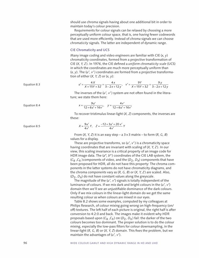
96 WIDE COLOUR GAMUT AND HIGH DYNAMIC RANGE IN HD AND UHD
should use chroma signals having about one additional bit in order to maintain today’s colour precision.
Requirements for colour signals can be relaxed by choosing a more perceptually uniform colour space, that is, one having fewer codewords that are used more efficiently. Instead of chroma signals we can choose chromaticity signals. The latter are independent of dynamic range.
CIE Chromaticity and UCS
Many image coding and video engineers are familiar with CIE (x, y) chromaticity coordinates, formed from a projective transformation of CIE (X, Y, Z ). In 1976, the CIE defined a uniform chromaticity scale (UCS) in which the coordinates are much more perceptually uniform than (x, y). The (u′, v′ ) coordinates are formed from a projective transforma-tion of either (X, Y, Z) or (x, y):
Equation 8.3
′u = 4 XX +15Y + 3Z
= 4 x3− 2 x +12 y
, ′v = 9YX +15Y + 3Z
= 9 y3− 2 x +12 y
The inverses of the (u′, v′ ) system are not often found in the litera-ture; we state them here:
Equation 8.4
x = 9 ′u12+ 6 ′u +16 ′v
, y = 4 ′v12+ 6 ′u +16 ′v
To recover tristimulus linear-light (X, Z) components, the inverses are these:
Equation 8.5
X = 9 ′u4 ′vY, Z = −12+ 3 ′u + 20 ′v
4 ′vY
From (X, Y, Z) it is an easy step – a 3 × 3 matrix – to form (R, G, B) values for a display.
These are projective transforms, so (u′, v′ ) is a chromaticity space having coordinates that are invariant with scaling of (X, Y, Z ). In our view, this scaling invariance is a critical property of an image code for HDR image data. The (a*, b* ) coordinates of the CIE LAB system, the (CB , CR ) components of video, and the (DZ , DX) components that have been proposed for HDR, all do not have this property: The chroma com-ponents in the latter systems do not have chromaticity diagrams, and the chroma components vary as (R, G, B) or (X, Y, Z ) are scaled. Also, (DZ , DX) do not have constant values along the greyscale.
The magnitude of the (u′, v′) signals is totally independent of the luminance of colours. If we mix dark and bright colours in the (u′, v′) domain then we’ll see an unjustifiable dominance of the dark colours. Only if we mix colours in the linear-light domain do we get the same resulting colour as when colours are mixed in our eyes.
Table 8.2 shows some examples, computed by my colleagues at Philips Research, of colour mixing going wrong on high-frequency (on/off) textures. The left half of each picture is original, the right half is after conversion to 4:2:0 and back. The images make it evident why HDR proposals based upon (CB , CR ) or (DZ , DX ) fail: the darker of the two colours becomes too dominant. The proper solution is to do the colour mixing, especially the low-pass filters for colour downsampling, in the linear-light (R, G, B) or (X, Y, Z) domain. This fixes the problem, but we maintain the advantages of (u′, v′).

CHAPTER 8 WIDE COLOUR GAMUT AND HIGH DYNAMIC RANGE IN HD AND UHD 97
Dark blue and lighter grey Light blue and very dark grey
Mix in (X, Y, Z ), linear-light
Mix in (Y′, CB , CR ), LDR
Mix in (Y′, CB , CR ), HDR
Mix in (Y′, DX , DZ ), HDR
Mix in (Y″, u′, v′), HDR
Transmit (Y″, u″, v″), HDR
Table 8.2 Example patches show the effect of chroma subsampling on high-frequency signal content. Ideally the subsampling would have no effect, and the left and right hand sides of each patch would appear identical. Many encoding schemes cause unwanted interference between luma and chroma, and distort the colours.
In practice, a slight modification to (u′, v′) is beneficial: Below a luminance of approximately 5 nt, the (u′, v′) signals are attenuated towards grey in proportion to Y″, forming signals denoted (u″, v″). These signals are amplified back at decoding. The scheme sends less dark colour noise to the MPEG encoder and has an insignificant effect on the perceived accuracy of dark colours. Said another way: In the region below 5 nt, (u″, v″) scale down with luminance just like 12-bit (CB , CR) signals do, so the accuracy is never worse.
This table summarizes the advantages of the scheme, compared to other proposals:
Table 8.1 Advantages and disadvantages of chroma and chromaticity signals
Chroma (CB , CR ) or (DZ , DX ) Chromaticity (u’, v’)
Grow with dynamic range, ≥ 12 bits per component needed
Independent of dynamic range, 10 bits needed
Multiple colour gamuts (dependent on RGB primaries), conversions needed
One infinite colour gamut, convert only once to the native display gamut
Inefficient code space, cube within a cube
Efficient code space, perceptually uniform
Sharpness loss for low-luminance colours when there is not much Y″ signal
All luminance sharpness is carried by the full bandwidth Y″ channel
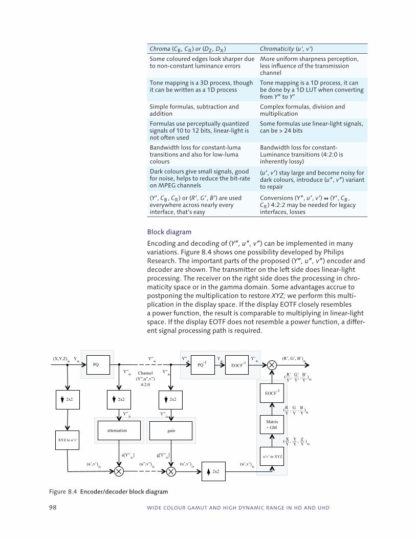
98 WIDE COLOUR GAMUT AND HIGH DYNAMIC RANGE IN HD AND UHD
Chroma (CB , CR ) or (DZ , DX ) Chromaticity (u’, v’)
Some coloured edges look sharper due to non-constant luminance errors
More uniform sharpness perception, less influence of the transmission channel
Tone mapping is a 3D process, though it can be written as a 1D process
Tone mapping is a 1D process, it can be done by a 1D LUT when converting from Y″ to Y′
Simple formulas, subtraction and addition
Complex formulas, division and multiplication
Formulas use perceptually quantized signals of 10 to 12 bits, linear-light is not often used
Some formulas use linear-light signals, can be > 24 bits
Bandwidth loss for constant-luma transitions and also for low-luma colours
Bandwidth loss for constant-Luminance transitions (4:2:0 is inherently lossy)
Dark colours give small signals, good for noise, helps to reduce the bit-rate on MPEG channels
(u′, v′) stay large and become noisy for dark colours, introduce (u″, v″) variant to repair
(Y′, CB , CR ) or (R′, G′, B′) are used everywhere across nearly every interface, that’s easy
Conversions (Y″, u′, v′) ↔ (Y′, CB , CR ) 4:2:2 may be needed for legacy interfaces, losses
Block diagram
Encoding and decoding of (Y″, u″, v″) can be implemented in many variations. Figure 8.4 shows one possibility developed by Philips Research. The important parts of the proposed (Y″, u″, v″) encoder and decoder are shown. The transmitter on the left side does linear-light processing. The receiver on the right side does the processing in chro-maticity space or in the gamma domain. Some advantages accrue to postponing the multiplication to restore XYZ; we perform this multi-plication in the display space. If the display EOTF closely resembles a power function, the result is comparable to multiplying in linear-light space. If the display EOTF does not resemble a power function, a differ-ent signal processing path is required.
Y4k
2x2
PQ PQ-1
Y”4k
Y4k
(u”,v”)2k
EOCF-1
Y’4k
Matrix + GM
2x2
Channel (Y”,u”,v”)
4:2:0
(X,Y,Z)4k
X Y Z (–– , –– , –– )
4k
Y Y Y
(R’, G’, B’)4k
EOCF-1
R G B (–– , –– , – )
4k
Y Y Y
2x2
Y”2k
Y”4k
2x2
Y”2k
attenuation gain
XYZ to u’v’
Y”4k
Y”4k
R’ G’ B’ (–– , –– , – )
4k
Y’ Y’ Y’
(u’,v’)2k
(u’,v’)2k
a[Y”2k
] g[Y”2k
]
(u’,v’)4k
u’v’ to XYZ
Figure 8.4 Encoder/decoder block diagram
CHAPTER 8 WIDE COLOUR GAMUT AND HIGH DYNAMIC RANGE IN HD AND UHD 99
Summary
We conclude that Y″CBCR (or Y″DZDX) is not optimum for HDR. Y″u″v″ is suitable. Compared to other schemes that have been proposed, a (Y″, u″, v″) 4:2:0 transmission signal for HDR promises a lower bit-rate, bet-ter colour reproduction at high spatial frequencies and 100% coverage of colour gamut.

100

101
9 Additive RGB and Colour Light Output (CLO)
At the heart of virtually all standards for digital colour image display is the principle of additive RGB mixture. According to this principle, col-ours are created by mixtures of specific red, green, and blue light. The mathematics of the mixture process are fairly straightforward, and the colours obtained are predictable. The scheme is inherent in the sRGB standard for desktop graphics and the BT.1886 standard for HD; the scheme applies to most direct-view displays and to many projectors.
However, in certain AMOLED displays and in certain projectors an engineering trade-off is made that optimizes the brightness of white at the expense of departing from the principle of additive mixture. The additive mixture principle does not predict the colours displayed on such displays; accuracy in reproducing the input signal suffers. Common display specifications make it difficult to determine whether a particular model of display uses this technique or not; furthermore, the commonly used method of specifying brightness allows nonadditive displays to claim a brightness advantage.
This chapter explains the principle of additive mixture. We‘ll provide graphic representations of additive and nonadditive colour mixture. We‘ll explain how display luminance is characterized – particularly in projectors – and we’ll detail the colour light output (CLO) metric that allows a user to determine what luminace a display can achieve without suffering the inaccuracy of nonadditive mixture.
Colour reproduction
Before introducing additive mixture, we set the stage with two brief dis-cussions: one discussion concerns colour accuracy, and the other estab-lishes the philosophical principle by which colour images are mastered.
In the early days of projectors, approximately the decade 1995 – 2005, sources of continuous-tone colour imagery were scarce. Scanners were expensive; digital still cameras were primitive; it ranged from difficult to impossible to use desktop computers to access video material. This was the era of “business graphics,” characterized by Power Point presentations comprising text, graphic elements, and clip art. Colour bar and pie charts were commonplace, but full-colour imagery was rare. The dominant attribute of digital projectors was brightness; for most users, accuracy wasn’t very important.
Around 2005, all that changed. Desktop scanners became easily and cheaply available; multi-function printers were commercialized having built-in scanners; digital still cameras proliferated. Capture and edit-
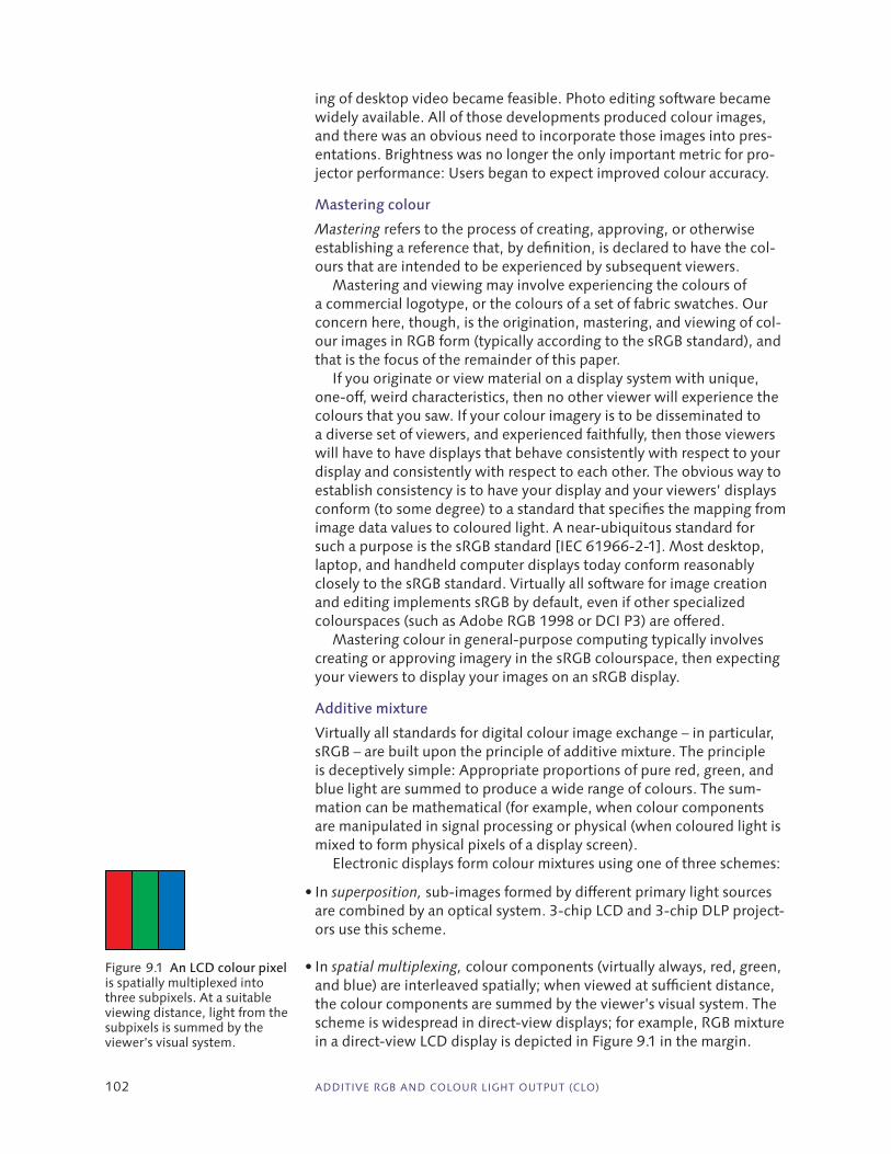
102 ADDITIVE RGB AND COLOUR LIGHT OUTPUT (CLO)
ing of desktop video became feasible. Photo editing software became widely available. All of those developments produced colour images, and there was an obvious need to incorporate those images into pres-entations. Brightness was no longer the only important metric for pro-jector performance: Users began to expect improved colour accuracy.
Mastering colour
Mastering refers to the process of creating, approving, or otherwise establishing a reference that, by definition, is declared to have the col-ours that are intended to be experienced by subsequent viewers.
Mastering and viewing may involve experiencing the colours of a commercial logotype, or the colours of a set of fabric swatches. Our concern here, though, is the origination, mastering, and viewing of col-our images in RGB form (typically according to the sRGB standard), and that is the focus of the remainder of this paper.
If you originate or view material on a display system with unique, one-off, weird characteristics, then no other viewer will experience the colours that you saw. If your colour imagery is to be disseminated to a diverse set of viewers, and experienced faithfully, then those viewers will have to have displays that behave consistently with respect to your display and consistently with respect to each other. The obvious way to establish consistency is to have your display and your viewers’ displays conform (to some degree) to a standard that specifies the mapping from image data values to coloured light. A near-ubiquitous standard for such a purpose is the sRGB standard [IEC 61966-2-1]. Most desktop, laptop, and handheld computer displays today conform reasonably closely to the sRGB standard. Virtually all software for image creation and editing implements sRGB by default, even if other specialized colourspaces (such as Adobe RGB 1998 or DCI P3) are offered.
Mastering colour in general-purpose computing typically involves creating or approving imagery in the sRGB colourspace, then expecting your viewers to display your images on an sRGB display.
Additive mixture
Virtually all standards for digital colour image exchange – in particular, sRGB – are built upon the principle of additive mixture. The principle is deceptively simple: Appropriate proportions of pure red, green, and blue light are summed to produce a wide range of colours. The sum-mation can be mathematical (for example, when colour components are manipulated in signal processing or physical (when coloured light is mixed to form physical pixels of a display screen).
Electronic displays form colour mixtures using one of three schemes:
• In superposition, sub-images formed by different primary light sources are combined by an optical system. 3-chip LCD and 3-chip DLP project-ors use this scheme.
• In spatial multiplexing, colour components (virtually always, red, green, and blue) are interleaved spatially; when viewed at sufficient distance, the colour components are summed by the viewer’s visual system. The scheme is widespread in direct-view displays; for example, RGB mixture in a direct-view LCD display is depicted in Figure 9.1 in the margin.
Figure 9.1 An LCD colour pixel is spatially multiplexed into three subpixels. At a suitable viewing distance, light from the subpixels is summed by the viewer’s visual system.

CHAPTER 9 ADDITIVE RGB AND COLOUR LIGHT OUTPUT (CLO) 103
• In temporal multiplexing (also called frame sequential colour), sub-im-ages formed by different colour components are arranged in time; when presented at a sufficiently high rate – when the set of all of the colour components is repeated every 1/60 s or less – the colour components are summed by the viewer’s visual system.
The three components of colour mixtures are analogous to the three coordinates of physical space, so we say that the range of possible col-our mixtures forms a colourspace. R, G, and B components are repre-sented in abstract terms in the range 0 to 1; the mixtures fill an RGB cube diagrammed in Figure 9.2. (Figure 9.3. will be discussed later.)
Different colours of red, green, and blue can potentially be chosen as the basis for colour mixtures; the individual pure components are called primaries. For pure colours and mixed colours to be consistent, the col-ours (technically, chromaticities) of the particular red, green, and blue primaries must be standardized. The sRGB standard defines the colour coordinates of specific red, green, and blue primaries. The BT.1886 colourspace for video and HD material [ITU-R BT.1886] has exactly the same primaries. Digital imagery is almost always prepared (mastered) with the sRGB/BT.1886 primaries; this scheme is almost certainly the one you are interested in when you’re distributing your images. sRGB/BT.1886 is bound to remain the dominant colourspace for the next dec-ade. The rest of this chapter focusses on sRGB/BT.1886 colours.
Figure 9.2 The RGB cube represents additive mixture of R, G, and B color components. Such a mixture represents sRGB image data values; it also represents physical mixture of RGB color components in the creation of colours on an sRGB display such as a projector. The display implements the color model of the color image data, consequently, faithful display of colors is achieved.
0.0
0.5
1.0
1.5
2.0
0.00.5
1.01.5
2.0
0.0
0.5
1.0
1.5
2.0
R
G
B
0.0
0.5
1.0
1.5
2.0
R
0.00.5
1.01.5
2.0
G
0.0
0.5
1.0
1.5
2.0
B
Figure 9.3 Various methods to “boost” white have been devised; these schemes cause nonadditive RGB mixture. Here, white is pushed to luminance 1.5 that of the sum of the individual R, G, and B luminance values; the high luminance at white is represented by the sharp point at coordinates [1.5, 1.5, 1.5]. The disadvantage is that colorspace is warped in a manner that doesn’t faithfully portray sRGB colors.

104 ADDITIVE RGB AND COLOUR LIGHT OUTPUT (CLO)
Light output
Users of direct-view displays and projectors are interested in light output – loosely, “brightness.” I say loosely because according to the governing body of colour science standards, the CIE, brightness is sub-jective; it cannot be measured. We can characterize a projector in terms of its total visible light output. To measure “brightness” of a projector, the appropriate quantity is luminous flux; its SI unit is the lumen [lm].
Flux is proportional to power; lumens [lm] are related to watts [W]. If a projector were to emit ultraviolet or infrared power, that power would not be perceptible, that is, not visually useful. The lumen is defined in a manner that mimics the spectral response of human vision: Ultraviolet and infrared power are weighted to zero, so ultraviolet and infrared power have zero luminous flux and measure as zero lumens.
The total emitted flux from a projector (in lumens) isn’t the whole story. Distance to the screen matters, as does the conversion of light illuminating the screen into light directed toward the viewers’ eyes. These issues involve luminance (which has its own unit, candelas per metre squared). See Units of ”brightness” in projection on page 121.
Light efficiency
Spectral distributions that are dominated by medium wavelengths (between about 500 nm and 600 nm) appear green. Human vision is more sensitive to those wavelengths than to wavelengths shorter than about 500 nm (which on their own appear blue) or to wavelengths longer than about 600 nm (which appear red). Green light dominates the calculation of light output.
A small desktop projector may have light output of 2000 lumens. Assuming that projector emits red, green, and blue light according to the sRGB/BT.1886 colourspace, about 1400 lm would come from the green channel, 425 lm from red, and just 175 lm from blue. Despite their low flux values, the red and blue light is critically important to colour: Although the blue signal produces a mere 7% of the total flux, without those 175 blue lumens there would be no blue in the pictures! Typically, around one third of the optical power (in watts) of a projector goes into producing just 7% of the light flux (in lumens).
In an ideal world, for the sake of faithful colour display, we would live with that trade-off. That would be the end of the story. However, in a quest for increased light output, some manufacturers sacrifice colour accuracy as we will now explore.
White boost
Display engineers found the very low flux of blue, and the fairly low flux of red, frustrating. Lots of electrical and optical power was consumed delivering those blue and red lumens. Display engineers were motiv-ated to obtain more lumens from a given amount of optical power. The maximum number of lumens per watt is obtained by using unfiltered or lightly filtered light – that is, using white or yellow light. Display engin-eers realized that if they included white light or yellow light in colour mixtures, efficiency could be improved: Colour mixtures could include “white boost” or “yellow boost.” (These terms are placed in quotes here because, although the techniques are widely used, the industry has no standard terms for the concept.)
Some people consider luminous flux to be comparable to energy. It’s not: Flux is related to the rate of flow of energy, that is, related to energy per unit time, that is, power. Lumens, not watts, are what you want when you buy a light bulb. European Union standards call for light bulbs to be advertised to con-sumers in lumens, not watts.
Quite a few years ago, ANSI standard-ized a measurement procedure for projectors [ANSI IT7.227]. Values measured according to that procedure came to be known (misleadingly) as ANSI lumens, even though no new unit was involved. In 2003, ANSI withdrew that standard. If you see ANSI lumens mentioned in any modern context, be suspicious. The comparable modern standard is ISO/IEC 61966-6.

CHAPTER 9 ADDITIVE RGB AND COLOUR LIGHT OUTPUT (CLO) 105
White boost in spatially multiplexed displays
In Figure 9.2, I presented an example of a spatially multiplexed display that delivers additive colour. Three spatially multiplexed direct-view displays having more than three components have been widely commercialized:
• Samsung’s PenTile RGBW scheme is used in several models of handheld devices. The scheme involves a white subpixel in addition to red, green, and blue. The white subpixel increases electrooptical efficiency com-pared to RGB; battery life is somewhat improved.
• Sharp Quattron direct-view LCD displays have a yellow subpixel in addition to the usual red, green, and blue: These displays do not have a white boost, they have a yellow boost. The scheme offers higher efficiency and slightly wider gamut than RGB LCDs; however, owing to nonlinear signal processing the colour mixture is non additive, so pre-dictability of colour suffers.
• LG OLED televisions use “white” OLED elements for all subpixels. Red, green, and blue filters are layered over three of the OLED subpixels; the fourth subpixel is left unfiltered. Although white boost would be pos-sible in such an arrangement, observation of the display suggests that white boost is not used. The algorithm is not public, but additive RGB is used. The minimum of the [R, G, B] values is computed. That value is subtracted from each of the R, G, and B drive signals, and the computed minimum drives the white OLED. A considerable power advantage is obtained. Ideally, the unfiltered white OLED spectral power distribu-tion is metameric to the sum of the filtered RGB; however even if it’s not metameric an appropriate mixture of RGB can be subtracted to compensate such that additive colour mixture is obtained.
Samsung PenTile scheme (spatial)
Sharp Quattron scheme (spatial)
LG RGBW OLED scheme (spatial)
3·
= 1.00.21263
0.71523
0.07223
+ +
3·
0.2126 0.7152+ +
Figure 5. In a white-segment (RGBW) projector, mixing red, green, and blue primary components makes white; however, additional light (dependent upon signal processing) is added from a fourth segment. The mixture becomes nonadditive. In this example, CLO remains 1, but the additional light “pushes” white light output (WLO) to 1.5.
0.21264
0.71524
0.07224
14
3·+ + +
= 1.53·
0.21266
0.71526
0.07226
1 0.21266
1 0.07226
16
3·+ + +−
+−
+ = 1.863·− −
Figure 9.4 A 3‑segment RGB 1‑DLP projector has red, green, and blue light presented sequentially to the modulator. The mixture is additive. The equation’s overall scale factor of 3 normalizes light output to 1; call this the normalized color light output.
Figure 9.5 A white‑segment (RGBW) projector mixes red, green, and blue primary components; however, additional light (dependent upon signal processing) is added from a fourth clear (“white”)segment. The mixture becomes nonadditive. In this example, CLO remains 1, but the additional light “pushes” white light output (WLO) to 1.5.
Figure 9.6 A 6‑segment (RGBCYW) projector has cyan and yellow segments in addition to the RGBW of the example above. White light output (WLO) is boosted to about 1.86 times the color light output (CLO); however, color accuracy suffers.

106 ADDITIVE RGB AND COLOUR LIGHT OUTPUT (CLO)
White boost in time‑multiplexed displays
Texas Instruments offers a light modulator called DLP that is used in projectors. Many DLP projectors – in particular, those used in digital cinema – have three light modulators (“3-chip DLP”), and achieve colour through the superposition scheme. Light from the light source is split into three wavelength bands, the bands are modulated separately, then recombined. These projectors exhibit additive mixture by design, and have accurate colour. In fact, in the case of digital cinema project-ors, they have very accurate colour.
In commercial and consumer use, single DLP (“1-chip DLP”) pro-jectors are common. Colour is created using the time-multiplexed (frame-sequential) scheme: Wideband white light is emitted by the projector bulb; red, green, and blue light is obtained time-sequentially from a filter wheel in the light path; and that light illuminates the DLP modulator.
A 1-chip DLP projector could, in principle, implement additive mixture. The filter wheel would insert a red filter into the light path for 1/3 of the time interval of each frame, a green filter 1/3 of the time, and a blue filter 1/3 of the time. This mixing scheme, depicted in Figure 9.4, would produce additive colour.
In a 1-chip DLP projector, “white boost” can be implemented by augmenting the red, green, and blue filter segments with a clear (“white”) filter segment. Signal processing circuits are used to “steer” a certain amount of the signal toward modulating the light correspond-ing to the white segment. The technique was described, though not called “white boost,” in a 1998 paper [Kunzman 1998]. The scheme is depicted in Figure 9.5.
A straightforward implementation of white boost shrinks the RGB segments of the filter wheel to 3/4 of their previous time intervals – to 1/4 red, 1/4 green, and 1/4 blue – freeing up 1/4 of the time for the white segment, as sketched in Figure 9.5. If the signal processing is arranged to drive the white segment fully when all of the R, G, and B signals are at their maximums, light output of this RGBW scheme would be 1.5 times that of the 3-segment RGB scheme.
Algorithms for “white boost” are usually secret.1 In a typical case, white boost produces white flux 1.5 times the sum of red, green, and blue. The algorithm could be as simple as this: If (R + G + B) ≤ 2, then set W to zero; otherwise, set W to (R + G + B) - 2. That algorithm pro-duces the RGB colourspace depicted in Figure 9.3 on page 103.
Many design variations are possible: The time interval of the white segment can be increased relative to the red, green, and blue segments; also, using more than four segments is possible. Some commercial projectors have red, green, blue, cyan, yellow, and white segments: RGBCYW. Figure 9.6 shows an example where white boost produces white flux about 1.86 times the sum of red, green, and blue. However, such design variations are typically accompanied by signal processing that causes nonadditive colour mixture.
Virtually all colours can be produced by mixtures of RGB. CMY seg-ments provide little to no benefit in the projected colour gamut if the colours produced are to remain additive (i.e., predictable).
1 An analysis of a commercial 1-chip DLP projector can be found in a paper by Heckaman and his colleagues [Heckaman 2006].

CHAPTER 9 ADDITIVE RGB AND COLOUR LIGHT OUTPUT (CLO) 107
Colour Light Output
To characterize the light output (total flux) of a greyscale projector, we could simply use lumens. However, most of us are more interested in colour projectors. For a projector that exhibits additive mixing, the calculation is trivially simple:
In additive colour mixture, total flux is simply the flux of the red component plus the flux of the green component plus the flux of the blue component, all measured in lumens.
However, we have seen that there are projectors whose colour mix-ing behaviour is far from additive. Such projectors are engineered to deliver lots of white light, but not as much red, green, or blue as would be required to exhibit additivity. Put simply, such projectors deliver “brightness” in certain colours, at the expense of colour accuracy.
Virtually all projector specifications include a specification of light output (in lumens); however, it can be difficult or impossible to deter-mine, from a spec sheet, whether a particular projector is designed to deliver additive mixture of RGB (that is, accurate colours) or not. The flux specification (lumens) applies to whatever mixture constitutes full white, including any “white boost” that is designed into the projector.
Until recently, there was no simple specification that could be quoted on a spec sheet that specified the “brightness” that could be achieved for accurate colour. Since the defining characteristic of an additive (accurate) projector is that white flux is the sum of the red, green, and blue flux values, the missing specification is straightforward:
Colour light output (CLO) is the sum of the flux of full red plus the flux of full green plus the flux of full blue, all measured in lumens.
A definition having this essence (but expressed in somewhat more technical language) was incorporated into the SID/ICDM IDMS stan-dard [2012 , Section 9.12, p 165]. The measurement methodology was described in detail by Kelley and his colleagues [Kelley 2009].
When CLO is quoted among the specifications of a projector, that value reveals the light output available for displaying accurate colours.
Total light output or white light output (WLO) may also be indicated. If white light output is higher than colour light output, then the pro-jector has “white boost.” A projector that implements white boost typ-ically affords access to a mode that switches off the boost, in order to achieve reasonable accuracy. The modes have no standard names, but the appropriate mode might be labelled srgb, theater, or photo. When these modes are activated, projector output drops significantly, by up to 40% of the projector’s marketed brightness level.
Summary
• Additive RGB is the foundation of digital imaging. The concept is sim-ple: White is the sum of red, green, and blue. Additive colour mixture is required by the sRGB standard for desktop colour and the BT.1886 standard for video.

108 ADDITIVE RGB AND COLOUR LIGHT OUTPUT (CLO)
• For colour fidelity, the colour characteristics of the viewers’ displays must be consistent with the characteristics of the source (master) display.
• Many digital projectors do not conform to the principle of additive colour mixture; in particular, “white boost” is common. It is not easy to identify, from a spec sheet, a projector with white boost or other depar-ture from reasonable colour accuracy.
• Colour Light Output (CLO) characterizes light output of additive colour mixture – that is, the light output of faithful colour (typically sRGB/BT.1886). If CLO is specified, the user is assured that the indicated light output (flux, in lumens) is available to faithfully display colour.

109
10 Contributions & conclusions
It is widely thought that the goal of digital imaging – including video and cinema – is to “reproduce,” at a display, the colour stimuli of a scene. Many textbooks explain that the goal is achieved by producing, at a display, luminance or colour tristimuli proportional to that of the scene. I have shown that assumption to be almost always wrong: Visual conditions almost always differ between the scene and the display – in particular, absolute luminance is usually lower at the display, and sur-round conditions usually differ – so an appearance match, not a match of the colour stimuli, is the behaviour that human viewers expect.
Adjustments in video acquisition and production are routinely made with reference to a mastering display and without direct reference to a scene. Consequently, the correct reference for distribution is not the scene, but rather the colour stimuli approved at the mastering display.
I will outline the contributions of this thesis in the sections below, where the section heads correspond to chapter titles.
Image acquisition and presentation
Many digital imaging engineers and scientists assume that the goal of digital imaging is to produce, at a display, light levels proportional to light levels at the original scene. Many imaging systems are described as accurately conveying image information from “scene-to-screen.” This thesis has shown that assumption to be wrong. Visual conditions (including absolute luminance and surround conditions) alter appear-ance. For a given colorimetric stimulus (such as XYZ or L*a*b*), when scene illumination levels are diverse (the usual case), or consumer pres-entation conditions are diverse (also the usual case), colour appearance changes. In professional imaging, it is faithful portrayal of appearance that matters, not faithful reproduction of colour stimuli. A successful imaging system must compensate for expected appearance changes.
I explained how approval of imagery at a mastering display is the ref-erence point for faithful presentation. Axiom Zero refers to this concept.
Colour management systems for graphic arts and digital photography are based upon input‑referred and output‑referred image data, but those systems were conceived for – and are effectively limited to – acquisition from scanned photographic media and presentation of reflective print media (having rather low contrast ratio and limited colour gamut). This thesis defined the term mastering‑display‑referred, and explained how that concept characterizes the image state of video data at mastering and distributed downstream from mastering. Such data carries explicit

110 CONTRIBUTIONS & CONCLUSIONS
or implicit information about visual conditions at mastering. Upstream of mastering, I described how a scene rendering transform is necessary to compensate for appearance shifts that would otherwise arise from variations in scene conditions. Downstream of mastering, when pres-entation conditions differ from mastering conditions, I described how a display rendering transform is necessary in order to compensate for appearance shifts that would be expected owing to diversity in displays and their viewing conditions.
Perceptual uniformity
It is a persistent source of confusion in digital imaging that the words intensity, brightness, and lightness are misused. This thesis clarified these terms and the underlying concepts.
Digital representation of image data is perceptually uniform if a small perturbation of a component value – such as the digital code value used to represent red, green, blue, or luminance – produces a change in light output that is approximately equally perceptible across the range of that value. I described how nearly all digital imaging systems have evolved to be tuned to vision’s nonlinearity in a manner that minimizes the number of bits per colour component. The issue is fundamental to the efficient storage and transmission of digital images; it is also funda-mental to “lossy” image and video compression, where it is vital that information be discarded in a manner that minimizes perceptibility. I explained how the tuning is mainly a consequence of technological natural selection and accidents of history; the fundamental issues of perceptual uniformity are largely unknown and the technical literature is rife with misunderstanding. I clarified the concept of perceptually uniform coding and detailed its relationship to CIE lightness.
Lightness mapping
The visual psychophysics literature has not established consensus on whether lightness perception follows Stevens’ Law (where lightness is assumed to follow a power law of luminance) or the Weber-Fechner Law (where lightness is assumed to follow a logarithmic law). This lack of consensus extends into the engineering of imaging systems: There are conflicting accounts in the literature, with some sources describing digital image systems as conforming to Stevens’ Law and other sources describing them as conforming to the Weber-Fechner Law.
I showed that optimum digital image encoding should conform roughly to Stevens (power) Law in the lower realms of relative lumin-ance (below about 10% of diffuse white), and conform roughly to the Weber-Fechner (logarithmic) Law in the higher realms. The thesis described how modern coding systems used in HD/UHD and digital cin-ema – for example, quasilog systems such as FilmStream, and “hyper-gamma” – conform to this interpretation.
Visual perception is modulated by the absolute luminance of colour stimuli: Colourfulness decreases as luminance decreases, even when chromaticity remains constant. However, imaging scientists and engin-eers ordinarily normalize image signals in the early stages of image acquisition and processing, and thereby discard perceptually meaning-ful differences in luminance. This normalization or scaling is so common that absolute luminance and relative luminance are often both sym-

CHAPTER 10 CONTRIBUTIONS & CONCLUSIONS 111
bolized Y. I showed that absolute luminance is fundamental to image appearance, and how it deserves its own letter symbol, L. I explained the importance of distinguishing and absolute luminance, relative luminance, and lightness, and I described the importance of carrying information about the overall scene illuminance into the imaging pipe-line to enable compensation of appearance effects.
Picture rendering in video/HD
It is very widely believed that a camera’s mapping from light to signal, and a display’s mapping from signal to light, should be inverses. Com-mon wisdom holds that a video camera converts light to signal accord-ing to a power function having an exponent of about 1/2.2 (about 0.45), and that a standard display converts signal to light according to a power function approximating a 2.2-power. I showed that the standard BT.709 camera encoding imposes an effective power of 0.5, not 0.45. The standard BT.1886 studio display imposes a power function having an exponent of 2.4, not 2.2. The ratio of 0.5 and 2.4 is 1.2: This thesis showed that a “factory setting” video/HD pipeline imposes a 1.2-power function from the scene to the mastering display. It is not referred to as such by the standards, but that end-to-end power applied to RGB tristimuli functions as a scene rendering transform.
In computing, a 2.2-power is standard (sRGB). Consumer television displays have no firm standards but “gamma” values are typically close to 2.2. I showed that the ratio of 2.2/2.4 (about 0.9) between these display conditions and the mastering condition has the effect of impos-ing a display rendering transform equivalent to a 0.9-power function on each of the R, G, and B tristimuli. I explained how application of this function is appropriate to compensate the higher luminance (about 320 nt diffuse white) and higher surround fraction (between 5% “dim” and 15 – 18% “average”) of these presentation conditions, compared to the mastering situation (100 nt and about 1% “very dim” surround).
I explained how appearance effects are compensated by signal processing in a process termed picture rendering. I showed that there are two distinct picture rendering transforms in professional imaging applications: the scene rendering transform and the display rendering transform. Because appearance depends upon both scene and display viewing conditions, scene-referred and display-referred image states must be distinguished. Many recent papers on HDR explain the import-ance of the optical-to-optical transfer function (OOTF). However, there are three important viewing conditions: scene, mastering, and consumer. This thesis explained why there are three important OOTFs – termed OOTF1 ,OOTF2, and OOTF3 – not one. Given the primacy of the mastering display in video distribution (Axiom Zero), only one of the three OOTFs – namely, OOTF2, as I term it – is important to video standards.
Contrast and brightness
Appearance effects in digital images have historically been partly compensated by contrast and brightness controls that are pro-vided by tools in the production pipeline (in modern systems, even Photoshop), and made available to end-users of display equipment. The words used to label these controls are terribly confused, and the
112 CONTRIBUTIONS & CONCLUSIONS
order of their operation, although reasonably consistent, is not widely understood. The deficiencies affect billions of consumers. I presented a numerical analysis of the signal processing associated with contrast and brightness processing and showed that the dominant effect of the contrast control is to alter visual brightness and that the dominant effect of the brightness control is to alter visual contrast. I explained why the appropriate user control to alter visual brightness is nei-ther contrast nor brightness, but the control labelled – completely nonintuitively – backlight.
Medical imaging
Medical imaging has, for the last 10 years or so, used perceptually uniform coding (dicom GSDF). However, medical imaging is primar-ily concerned with the preservation of just-noticeable-differences in image data values, and is not very concerned about the appearance of large luminance differences. Consequently, the coding and processing of medical image data is somewhat different from that of other appli-cations of imaging. I explored those differences, and presented the mathematics underlying medical display calibration.
Wide colour gamut and high dynamic range
The most important practical application of appearance modelling in video is in high dynamic range (HDR) and wide colour gamut (WCG) systems. I analyzed the application of the principles described in this thesis to a commercially feasible HDR/WCG imaging system.
Summary
I have described how colour appearance effects arise in digital imaging. These effects potentially appear in two places: first, between a scene and a mastering display; and second, between a mastering display and a consumer display. Compensation for such appearance effects is neces-sary to make images look the same, even if colorimetric measures then differ. Compensation is almost always required in commercial imaging systems, but has not previously been studied systematically for digital media. In this thesis, I have shown that in modern HD/UHD practice, appearance effects between the scene and the mastering display are compensated by having “gamma” values in the camera and at the mastering display that combine to impose a 1.2-power function of RGB tristimuli. This power function has been described in prior literature as being required owing to “non-ideal” behaviour of various system com-ponents, but I argue that it is fundamental. I have described how the typical consumer display and sRGB “gamma” value of about 2.2, when applied to image data from from a standard mastering display, yields an appearance transform suitable for the consumer display and viewing conditions. I have framed the discussion in terms of HD/UHD, but such transforms are required in HDR between black and the diffuse white (as portrayed).
In summary, I have bridged between visual psychophysics, colour appearance theory, and the practice of image signal acquisition, pro-cessing, storage, transmission, and display in modern digital imaging systems.

113
Appendices
A Essential terms & concepts of picture rendering 115
B Seeing the light: Misuse of the term intensity 119
C Review of perceptual uniformity and picture rendering in video 123
D References 129

114 APPENDICES

115
A Essential terms & concepts
of picture rendering
This glossary describes terms relating to image appearance that are important to signal processing in professionally produced digital cinema and video/HD/UHD, and described in the body of the thesis. I assume familiarity with HD terminology, as covered in the Glossary of Poynton [2012].
Absolute scene-referred Scene-referred image data where image signal values or associated metadata convey estimated absolute luminance in the scene, such as the relation between signal value and the absolute luminance of an 18%, 90%, or other diffuse reflector in the scene under the dominant scene illuminant. According to ST 2065-1, ACES image data is supposed to be absolute scene-referred with a diffuse white luminance of 1 600 nt; however, in practice ACES image data is nearly always relative scene-referred.
Axiom Zero (A0) “Faithful (authentic) presentation is achieved in video/HD/UHD/D‑cinema when imagery is presented to the consumer in a man‑ner that closely approximates its appearance on the display upon which final creative decisions were approved.”
Axiom Zero, Corollary Zero (A0C0) “The original scene – if there is one – is not the reference point for faithful presentation.” The original scene is not the reference point for image fidelity for several reasons: [a] imagery may be synthetic (there may be no original scene); [b] col-ours in the original scene may be clipped or otherwise transformed to lie within the colour gamut of recording, mastering, distribution, and/or presentation; [c] the tone scale of the scene may be reduced or expanded for technical or artistic reasons; [d] arbitrary colour manipula-tion for artistic purposes may legitimately intervene between the scene and the mastered content; and [e] image data is typically transformed to achieve an approximate appearance match between the scene and the display (which is typically not nearly as bright as the scene and is typically viewed in a dim or dark surround).
Axiom Zero, Corollary One (A0C1) “When accessing mastering‑dis‑play‑referred material, it is reasonable to infer the director’s experience at the time of content approval; however, intent cannot be inferred object‑ively at the time and place of presentation.”
Axiom Zero, Corollary Two (A0C2) “To declare video to be scene‑referred is to restrict or eliminate artistic freedom in choosing tone or colour in production and postproduction.”
116 ESSENTIAL TERMS & CONCEPTS OF PICTURE RENDERING
Colour appearance According to CIE, “aspect of visual perception by which things are recognized by their colour.” Colour is in the human eye and brain; it is not a completely physical phenomenon. Colour appear-ance, as used in digital imaging, refers to the variability of perceived colour of a physical stimulus (target), or its portrayal on a display, taking into account aspects of the visual stimulus and elements surrounding it in the visual field, including absolute luminance, object shape, angular subtense, visible texture, and spatial frequency.
Diffuse white The absolute or relative luminance reflected in a Lam-bertian (nonspecular) manner by a white surface under nondirectional illumination; the digital representation of that luminance; or the abso-lute or relative luminance of the portrayal of that surface on a display. Under ordinary lighting, a diffuse white surface has a relative luminance (or luminance factor, or diffuse reflectance, or albedo) of around 0.9.
Director’s intent, Creative intent See Axiom Zero. Display-referred Image data wherein intended appearance is obtained
through a documented mathematical mapping from signal value to absolute colorimetric light at the surface of a particular display viewed in a particular, specified viewing condition.
Display rendering Signal processing applied at display equipment downstream of mastering to compensate for visual appearance effects owing to differences between mastering display conditions in the mas-tering viewing environment and presentation display conditions in the presentation viewing environment (e.g., at a consumer’s premises). Dis-play rendering is typically not required in digital cinema because display characteristics and viewing conditions at presentation (“exhibition”) closely match display and viewing conditions at mastering. In HD, display rendering is referenced to the studio reference display, which according to BT.1886 closely approximates a pure 2.4-power function and according to ST 2080-1 delivers 100 nt reference white. HD mas-tering is typically performed in a very dim surround of about 1 nt (1% of diffuse white). An appearance match on a brighter display in a brighter environment (e.g., sRGB as practiced, with reference/diffuse white portrayed at around 320 nt) requires a lower display power-function exponent (“gamma”) of around 2.2 – that is, display rendering is associ-ated with a power-function having an exponent of about 2.2/2.4 = 0.9. An appearance match on a darker display in a darker environment (e.g., d-cinema, with diffuse white portrayed at about 32 nt) requires a higher display power-function exponent (“gamma”) of around 2.6/2.4 = 1.1; that is, display rendering is associated with a power-function having an exponent of about 1.1.
Faithful/authentic presentation See Axiom Zero. Faithful presentation of professionally created material is defined with respect to the experi‑ence (not the “intent”) of the creative group that mastered the content.
Image state Information concerning display and viewing conditions that is necessary to enable reconstruction of image appearance from colorimetric image data. Key parameters include the chromaticity and absolute luminance of diffuse white and the chromaticity and absolute or relative luminance of the surround. In digital video/HD/UHD or d-cinema, image signal values are categorized as either scene‑referred (typically associated with average luminance of 320 nt or more) or dis‑play‑referred (typically associated with average luminance of 100 nt or

APPENDIX A ESSENTIAL TERMS & CONCEPTS OF PICTURE RENDERING 117
less). Display-referred image data can be distinguished as mastering‑dis‑play‑referred or referred to consumer display conditions.
Mastering-display-referred Image data wherein intended appearance is obtained, or creative decisions were finalized, through a documented mathematical mapping from signal value to absolute colorimetric light at the surface of a standardized display (e.g., for HD, according to BT.1886 and SMPTE ST 2080-1) as viewed in a particular specified or standardized viewing condition.
Physical contrast The ratio of a higher luminance value and a lower luminance value; possibly a ratio near unity (e.g., Weber ratio), a mod-erate ratio, or a large ratio (e.g., contrast ratio). Physical contrast is meaningful only when referenced to physical (optical) light levels.
Picture rendering Signal processing to compensate for visual appear-ance effects owing to the ratio (often a factor of 1000 or more) in absolute luminance between diffuse white in a real or imagined scene and its portrayal on a display, transforming from scene-referred image data into display-referred image data. For professionally mastered content, picture rendering conceptually involves the concatenation of scene rendering and display rendering transforms. Picture rendering transforms are sometimes explicit, for example in ACES, where there are explicit rendering (RRT) and display (ODT) transforms. Picture render-ing transforms are sometimes implicit in the concatenation of various transforms, for example in HD, where scene rendering is the concaten-ation of the camera’s OETF as adjusted, any processing alterations (e.g., in colour grading), and the display’s EOTF.
Poynton’s Fourth Law “Downstream of program mastering, errors in production are indistinguishable from expressions of creative intent.”
Presentation (portrayal, depiction) The process of converting image data to coloured light on a rectangular surface and optically conveying that light to the eyes of one or more observers. Presentation is distin-guished from the scene, and distinguished from the optical image of the scene on a sensor surface (the focal plane image).
Raw In digital photography, scene-referred image signal values – that is, image signal values absent any scene or display rendering transforms. Raw data may be radiometric or processed by a nonlinear OETF, and may be uncompressed or compressed. Raw data is typically in mosaic (“Bayer”) form, but may be demosaicked.
Relative scene-referred Scene-referred image data where signal values convey estimated relative tristimulus values. (In relative-scene-referred image data, absolute luminance reference is not directly available.)
Rendering Image data manipulation to achieve a desired image appearance.
Rendering intent The term is best avoided in digital video/HD/UHD or d-cinema. 1. In ICC desktop and graphics arts colour management, metadata indicating colour treatment to render image data from the ICC profile connection space (see ISO 15076-1:2005) onto a device having certain gamut and/or viewing conditions. 2. In BBC HLG ter-minology, and BT.2390 terminology, picture rendering. In 2003, when image colour appearance terminology was in development, Poynton [2003] used the term rendering intent; in Poynton’s second edition [2012], that term was replaced by picture rendering.

118 ESSENTIAL TERMS & CONCEPTS OF PICTURE RENDERING
Saturation Ambiguous. 1. Colour saturation: Colourfulness relative to lightness; the degree to which a colour is judged to be free from mix-ture with white. Colour purity. 2. Sensor saturation: A condition where the magnitude of an optical stimulus exceeds the capacity of an image sensor element. 3. Signal saturation: A condition where an image signal is at the higher limit of its ability to represent optical magnitude. 4. Saturation: A user-accessible control that adjusts chroma of image signal values; more sensibly called chroma.
Scene-referred For image data that is acquired from or otherwise intimately connected to a scene, the property of having a documented mathematical mapping from estimated colorimetric light (e.g., absolute or relative luminance, or tristimuli) to image signal value. Image signal value may be referenced to the scene directly, or may be referenced to the image (focal) plane of the sensor, in which case optical flare may be incorporated. In digital still photography, scene-referred image data is known as “raw.” Image data cannot be scene referred if any of the following conditions hold: [a] camera signal tone or colour mapping algorithms are unknown or undocumented; [b] camera adjustments apart from exposure or gain are made without being accompanied by documented algorithms and associated metadata; or [c] camera signal processing imposes significant gamut limitation with respect to the Pointer [1980] gamut, such as clipping to BT.709 gamut.
Scene rendering Signal processing to compensate for visual appearance effects owing to the ratio (often a factor of 1000 or more) in abso-lute luminance between diffuse white in a scene and its portrayal on a mastering (studio reference) display. In HD, scene rendering is usually effected by the combination of the camera’s OETF (where the BT.709 standard OETF approximates a 0.5-power of scene tristimulus values) and a standard studio reference display in a known viewing condition (e.g., for HD, the pure 2.4-power function standardized by BT.1886 combined with 100 nt reference white luminance standardized by ST 2080-1 and approximately 1% surround ratio). For HD, an “end-to-end” power function (OOTF) exponent of approximately 1.2 results, suitable for scene diffuse white of about 3200 nt. (The terminal “end” in this case refers to the mastering display, not to a consumer display.)
Screen-referred Please avoid this term; use display‑referred. Because “screen-referred” is nearly a homonym of scene-referred, it is poten-tially confusing.
Visual contrast The apparent (subjective, qualitative) difference, large or small, between two luminances or colours as judged by human vision.

119
B Seeing the light:
Misuse of the term intensity
Many common words used to describe light – such as lightness, bright‑ness, intensity, and value – have special meanings in the technical domains of physics, optics, and colour science. In popular writing, lack of precision is understandable: To impose rigour on the beginner would deter understanding, not aid it. However, in technical sources such as textbooks and journal articles, lack of rigour is a serious flaw. Much image processing and video research is reported where it is impossible to determine from the published results whether the investigators were using pixel values that were physically linear or pixel values that were perceptually uniform. In this note I will set out several misused terms, and try to set straight some of the misunderstandings of the term with respect to digital imaging.
Intensity
Luminous intensity is one of the seven basic SI quantities. To be included among the seven base SI quantities, intensity must be import-ant ! Nonetheless, the term is widely misused in computer graphics, video, and other domains. Palmer [1993] lamented poor use of the term within the field of optics.
Intensity is flux – that is, power – per unit solid angle. The SI unit for power is the watt [W]; the SI unit for solid angle is the steradian [sr]. The SI unit for radiant (electromagnetic) intensity is watts per steradian [W / sr, or as I prefer to write it, W · sr −1].
Intensity refers to flux emitted in a particular direction into a cone of infinitesimal “width” (or properly, solid angle). The reference solid angle corresponds to quite a broad cone, about 65.5° in diameter. However, expressing flux per steradian doesn’t require measuring across a whole steradian any more than you have to wait an hour to measure 55 mph, or wait a second to measure speed of 24.5872 m · s −1. The physics and mathematics of this concept (and its unit) is that emitted flux in a par-ticular direction is characterized without having to express the cone angle over which it was measured.
Intensity captures a source property from a distance. Intensity is defined so as to neutralize the inverse square law.
Radiometry deals with radiant intensity, whose units are watts per steradian (W · sr −1). In photometry, the spectral intensity of radiometry is weighted by the spectral sensitivity of human vision – the V(λ), also

120 SEEING THE LIGHT: MISUSE OF THE TERM INTENSITY
known as y(λ) – function of the CIE. Photometry deals with luminous intensity, whose units are candelas [cd], equivalent to lumens per stera-dian [lm · sr −1]. Luminous intensity is appropriate to characterize the visible light output, in a specified direction, of a point-like source.
In image science, we are generally concerned with area-like sources. We need to include area in our units. Radiance is intensity per unit (pro-jected) area; the SI derived unit is watts per steradian per meter squared [W · sr −1 · m −2]. To characterize radiance that has visual effect, we weight by V(λ); the quantity is luminance, its SI derived unit is candela per meter squared [cd · m −2], often colloquially called nit [nt].
Intensity is by definition proportional to physical light power; it is what I call a linear‑light quantity.
Misuse of intensity
Nearly all image sensor devices (CCD and CMOS imagers) respond linearly to light power; however, in-camera processing typically sub-jects sensor values to a nonlinear mapping to produce pixel values. (For example, the camera may impose “gamma correction.”) The mapping typically approximates the human visual response to light power – that is, “gamma correction” approximates the CIE L* function. Pixel values are typically not proportional to light power; instead, they are typically coded in accordance with perceptual properties: pixel values are typ-ically perceptually uniform.
The primary misuse of the term intensity involves using the word to describe pixel values independent of their relationship to the underlying physical quantities, and in particular, using “intensity” to denote perceptual quantities that are not proportional to light flux. For example, it is common to use the word intensity to describe pixel values in image processing software. For its first two decades, until version 5, the matlab system used the term “intensity image’; however, pixel values in matlab images are ordinarily proportional to displayed intensity raised to approximately the 0.42-power. The same situation pertains for Mathematica: The built-in symbol GrayLevel specifies what Mathematica calls “the gray-level intensity”; however, like matlab, pixel values in Mathematica images are ordinarily proportional to displayed intensity to the 0.42-power. It is common to use the word intensity to describe RGB values in computer graphics – for example, RGB values in a colour lookup table (CLUT). However, those colourmap entries are actually perceptually uniform values (properly denoted R’G’B’, where the primes denote the nonlinearity with respect to physical power). In the ICTCP coding standardized in BT.2100 for HDR video, the I stands for “intensity” – but the associated signal is perceptually coded, not radiometric.
A secondary misuse of intensity relates to the absence of area from its definition. Intensity characterizes light power emitted from a point-like source in a particular direction. In digital imaging we are ordinarily concerned with area-like sources, where characterization of power should be given per unit area. For example, a display screen is not char-acterized in candelas, the unit of luminous intensity, but in candelas per meter squared.
A third misuse of intensity relates to the fact that spectral content is absent from its definition in physics. This tertiary misuse of intensity

APPENDIX B SEEING THE LIGHT: MISUSE OF THE TERM INTENSITY 121
arises from use of the term to describe visible light. Only a small part of the electromagnetic spectrum is visible ! If the adjective luminous is prepended, then the spectral weighting of is the CIE Standard Observer is meant; however, imaging systems rarely use cameras that accurately sense colorimetric quantities; usually, the best that is possible is to have an approximation of luminous intensity.
Units of ”brightness” in projection
In the language of video and data projectors, the term “brightness” is used very loosely; according to the CIE, brightness can’t even be quan-tified! This section outlines how luminous power (flux) emitted from a projector is converted to luminance, the quantity that describes the visual effect of light in transit from the display surface to the viewers’ eyes.
Flux characterizes light output of a projector. The screen is located at some distance from the projector, and light falls off as the inverse of the square of that distance. When a given amount of flux fully illuminates a display screen – that is, when an appropriate combination of lens and viewing distance is used – then the illuminance incident on the screen is the flux divided by the screen area. The appropriate SI unit is lux [lx]; one lux is a lumen per metre squared.
The visual sensation of brightness of an image element isn’t deter-mined by the flux or illuminance, but by the flux emitted from a small area of the image into a narrow beam directed toward the viewer’s eyes. To characterize the amount of light experienced by a viewer, the appropriate quantity is luminance, having units of candela per metre squared. Luminance quantifies light emitted from a direct-view display such as an LCD or AMOLED, or light reflected from a projector screen toward a viewer.
Assuming for the moment that the screen is perfect – what a colour scientist would call a perfect diffuse reflector (PDR) – the conversion of illuminance into luminance can be computed in SI units: Just divide illuminance (in lux) by π to obtain luminance (in nits).
In practice, a screen may have reflectance less than unity, or – if it has gain – effective reflectance greater than unity. To incorporate screen loss or gain, just use the appropriate factor (typically between 0.7 and 1.5).
Illuminance is a function of screen area. An image 1.33 m wide and 0.75 m high has an aspect ratio of 16:9 and an area of 1 m2; its image diagonal will be sqrt[1.332 + 0.752], or about 1.5 m (60 in).
Take the example of projector having 2000 lumens fully illuminating a 4 m2 unity-gain screen. You can expect screen illuminance of 2000 lm divided by 4 m2, that is, 500 lx. Divide that value by π to obtain lumin-ance; in this case, 160 nt. A modern desktop LCD display set to full brightness has luminance of about 320 nt: For this projector, you’ll want lighting that is somewhat subdued compared to that of an office environment. If you want luminance comparable to a desktop display, you’ll need flux of about 4000 lm. Projector manufacturers and system integrators often offer spreadsheets and web pages that perform such calculations. Beware projectors having white light output (WLO) larger than colour light output (CLO); such projectors have colour distortion.
Screen gain greater than one can only be obtained from a non-diffuse reflector: When screen gain is greater than unity, viewing angle is necessar-ily restricted to some extent.

122 SEEING THE LIGHT: MISUSE OF THE TERM INTENSITY
Recommendations
• Use intensity to describe physical quantities that are that are propor-tional to light power and expressed per unit solid angle. If you don’t understand solid angle and steradians, then avoid the term.
• Use radiance and luminance to describe physical quantities that are pro-portional to light power and are expressed per unit solid angle, per unit projected area. If you don’t understand solid angle, steradians, and projected area, then be careful using these tersm.
• Use primes on quantities such as R’, G’, B’, and Y’ when the correspond-ing quantities are perceptually coded, as in video, JPEG, and MPEG, and in most raster image files such as GIF, BMP, and TIFF.
123
C Review of perceptual uniformity
and picture rendering in video
Digital image encoding is perceptually uniform if a small perturba-tion to a component value – such as the digital code value used to encode luminance, red, green, or blue – is approximately equally perceptible across the range of that value. Perceived lightness follows approximately a 0.42-power function with respect to luminance (which is, by definition, physical). The most effective use is made of a limited number of bits per component when coding approximates lightness.
Picture rendering refers to modifications to image data that are made in order to obtain subjectively correct reproduction under display and viewing conditions different from capture conditions.
Although the principles of perceptual uniformity and picture ren-dering are used in virtually all commercial imaging systems, their use in video is widely unknown or misunderstood. This appendix surveys the development and deployment of these concepts in video, from their origins in the 1930s to their contemporary use at present. Poyn-ton [2012] surveys contemporary use of these concepts.
The following discussion assumes that you are familiar with colour science and with the basic concepts of video systems, and that you are familiar with video terminology. An introduction to the technical issues of perceptual uniformity is provided in Chapter 3, on page 11, and in Digital Video and HD Algorithms and Interfaces [Poynton 2012]
History of perceptual uniformity
Perceptual uniformity in electronic imaging was appreciated almost three quarters of a century ago. In 1939, Maloff [1939] wrote this about black and white television:
A small increment in light intensity is more noticeable to the eye in dark parts of the picture than is the same increment in bright parts of the picture. When the picture at the receiver is expanded,1 the highlights are over‑emphasized and shadows are under‑emphasized, and in this way a greater amount of interfer‑ence may be tolerated. … The expansion or increase in contrast may be applied either at the transmitter or the receiver, but the
1 The “picture” (really, luminance range) is “expanded” (increased) by the CRT’s power function, whose exponent is larger than unity.

124 REVIEW OF PERCEPTUAL UNIFORMITY AND PICTURE RENDERING IN VIDEO
interference consideration makes it more desirable to expand at the receiver.
In his book about monochrome television, Fink [1940] summarized the relationship of image coding and perceptual uniformity. Concerning the 525-line monochrome standard, established in 1941, he said:
The transmitter output shall vary in substantially inverse logarith‑mic relation to the brightness [now, luminance] of the subject.
The “logarithmic relation” reflects the Weber-Fechner law, which was detailed by Fink. The reference to “inverse” concerns the transmitter’s negative modulation polarity, which is irrelevant to our purposes.
In 1950, during development of the NTSC colour system, Mertz [1950] published a comprehensive description of the issue. He con-cluded (using the symbol n instead of today’s γ):
The characteristic for n = 1 gives … the greatest susceptibility to additive noise. … As n is increased, the susceptibility to additive noise is reduced … The changes are slow beyond n = 2.
Had Mertz explored values of γ much beyond 3, he would have found noise in the whites.
In 1950, the noise was analog – what Maloff called “interference,” and what Mertz called “random.” Nowadays, in digital systems, the noise arises from quantization. However, whether noise arises from analog or digital processes, the effects are similar. What Mertz describes as “characteristic for n = 1” we would today term linear‑light.
CRTs of Mertz’s day had power laws of about 2.3 ~ 2.5, and were appreciated in his time to be well matched to perception. In his 1950 paper “Tone Rendition in Television,” Oliver [1950] gave quite a lucid summary of the Weber-Fechner law applied to luminance, then stated:
With a 2.5‑root transmitter, a 2.5‑power receiver, properly adjusted, would give linear reproduction … any receiver exponent lying between 2 and 3 is not too bad a match [to perception].
Applebaum [1952] clearly expressed the desirability of nonlinear pro-cessing in terms of vision:
The brightness‑transfer characteristic of the average picture tube compresses the shadow tones and expands highlight tones. How‑ever, it has been shown that the nonlinear characteristic of the average picture tube is almost ideal for minimizing noise sensitiv‑ity. This indicates that the precorrections for the nonlinear charac‑teristic of the receiver should be applied at the transmitter …
The FCC standard for NTSC [U. S. Reg. Title 47, p 212] refers to R, G, and B signals
… having a transfer gradient (gamma exponent) of 2.2 associated with each primary color.
The parenthesized words are in the original. The standard fails to describe whether the 2.2 value refers to the reciprocal of the effective power function exponent at the encoder (what I term γ e ), or to the effective power function exponent at the decoder (γ d).

APPENDIX C REVIEW OF PERCEPTUAL UNIFORMITY AND PICTURE RENDERING IN VIDEO 125
The FCC avoided placing a tolerance on gamma:
Note: At the present state of the art it is considered inadvisable to set a tolerance on the value of gamma ...
Apparently the issue was not sufficiently well understood in 1953 to standardize a firm number. The FCC has never revisited the issue.
NTSC was thereby standardized with decoding having an exponent of somewhere around 2.2, expecting encoding at the camera through a power function having an exponent of somewhere around 1/2.2 (gamma correction). In practice, decoding must have used the power function intrinsic in CRTs of the day, which I suspect had exponents around 2.3 or 2.4. Encoding would have been done with whatever function made the best looking pictures on such a display.
The Hazeltine Labs book [Hazeltine 1956] states:
… it is very benificial from the standpoint of combatting radio‑path noise to have the receiver compress the dark shades and expand the light shades. The usual picture tube, either mono‑chrome or color, has a characteristic in the right direction in this regard.
The passage refers to “radio-path noise”: additive white Gaussian noise (AWGN) in the RF channel was the dominant noise source at the time. The perceptual coding that was effected by the power functions at the encoder and decoder caused noise to be distributed approximately uniformly across the tone scale from black to white.
The 2.2 figure – again without reference to whether it is intended for encoding or decoding – is documented in ITU-R Report 624 [ITU BT.624].
Many European video engineers expect the decoder gamma (of a studio display or a television receiver) to be 2.8: That value was enshrined in EBU standards, and is documented in ITU-R Rep. 624. I have found no evidence that such a high value has ever been used. To the contrary, Alan Roberts found values of the exponent in Europe between 2.2 and 2.4 [Roberts 1993], quite consistent with the 2.4 value found in North America.
The seminal documents of the NTSC used the term luminance signal. Judging from their published work, the participants in the first decade clearly understood that the signal was not linearly related to colour science luminance. However, over the following several decades the distinction was lost to almost everyone involved in video engineer-ing. Despite its rigid definition in the colour science community as a linear-light quantity, the term luminance came to be used by the video engineering community to reflect the nonlinear quantity representing the achromatic signal. Confusion resulted. The confusion is discussed in Appendix A of Digital video and HDTV algorithms and interfaces [Poynton 2012]. The sloppy nomenclature made its way into ostensibly authoritative video references, such as Pritchard’s SMPTE paper [1977].
History of perceptual uniformity in computer graphics
Computer graphics pioneers recognized early on the importance of per-ceptual uniformity (although they did not give it that term – or indeed, any particular term). Tom Stockham, at the University of Utah, analysed

126 REVIEW OF PERCEPTUAL UNIFORMITY AND PICTURE RENDERING IN VIDEO
the situation very thoroughly in a 1972 paper [Stockham 1972], and detailed the advantages of logarithmic coding. Shortly afterward, that university became a hotbed of computer graphics development. Edwin Catmull – later to found Pixar – attended that university, and in 1979 characterized the transfer of computer images to film; he considered perceptual requirements, but used the word “intensity” quite loosely) [Catmull 1979].
Alvy Ray Smith joined Catmull at NYIT. In his quest to adapt video principles to computer graphics, Smith apparently encountered the word luminance (presumably from Pritchard’s paper). Smith apparently correlated Pritchard’s use of the term luminance with his own know-ledge of the term as used in colour science. Understandably – though wrongly – he concluded that video “luminance” and colour science luminance were identical. His 1978 paper [Smith 1978] clearly pre-sented “NTSC luminance” as a linear combination of RGB. So, percep-tual uniformity was appreciated, but it was mistakenly not understood to extend to video. Smith’s conclusions were published in the highly influential proceedings of the siggraph conference.
It took only a few years for Smith’s interpretation to pervade com-puter graphics. The seminal textbook by Foley and van Dam states, without attributing any primary sources [Foley 1984],
The Y component of YIQ is not yellow but luminance, and is defined to be the same as the CIE Y primary.
Foley and van Dam discuss the desirability of an exponential relation-ship between RGB digital code values and the associated tristimulus values (“intensities”), thereby suggesting a logarithmic relationship between “intensities” and code values. However, like Smith, they fail to extend this concept to video, and wrongly describe video as having linear-light coding. Foley and van Dam cite Pritchard’s 1977 paper. Clearly, Pritchard’s failure to properly describe video’s “luminance” contributed strongly to subsequent misunderstanding.
Foley and van Dam subsequently revised their book into several editions (adding co-authors Feiner and Hughes), and unknowingly propagated the error. The die was cast. Confusion was to reign for the next few decades. With the emergence of colour management systems around 1995, colour science concepts and terminology reached a broad audience among computer professionals, and – perhaps a decade later – a broad audience among video professionals. Only since 2005 or so has the confusion begun to subside.
History of picture rendering in video
Well before the invention of the NTSC colour system, the necessity of picture rendering – then termed “modification to the tone scale” – was appreciated for monochrome television. Maloff stated [1939],
Unity gamma is not sufficient for transmitting studio and outdoor pickup and for such occasions the contrast should be raised [to achieve a2] resultant overall contrast of 1.6.
2 The phrase in square brackets is mine.

APPENDIX C REVIEW OF PERCEPTUAL UNIFORMITY AND PICTURE RENDERING IN VIDEO 127
The high value of 1.6 is presumably due to displays of the time being rather dim.
Fink’s 1940 book [1940] contains this passage:
An over‑all value of gamma of between 1.2 and 1.7 is used in commercial motion pictures … similar values of gamma should serve equally well for television work.
Maloff’s terms “unity gamma” and “resultant overall contrast” and Fink’s term “over-all value of gamma” all refer to the end-to-end power function exponent – the product of the gamma exponents at each stage. Today, some people call this “system gamma.” Decades ago, the “system” comprised just a few subsystems between the original scene and eventual presentation; in that era, the term “system gamma” was unambiguous. Now, many subsystems intervene between capture and display, and many people use the term “system gamma” to refer to the power function imposed by an individual subsystem, thereby intro-ducing ambiguity and confusion. Lacking a clear delineation of what constitutes the “system,” I avoid the term.
The 1953 U. S. FCC standard for NTSC [U. S. Reg. Title 47, p 212] refers to R, G, and B signals … having a transfer gradient (gamma expo-nent) of 2.2 associated with each primary color.
Describing the NTSC colour system, the famous Hazeltine book cited in the margin [Hazeltine 1956] states:
… typical conditions might include a [gamma] corrector adjusted to an exponent of 0.64 (= 1⁄1.6 ), which will reduce the 2.2 of the picture tube to 1.4 for the system.
I find Hazeltine’s quoted CRT exponent of 2.2 somewhat low. Some accounts of the time quote CRT exponents as high as 2.75. Bingley’s 1954 paper [1954] on transfer characteristics discusses, on page 75, an encoder having an exponent of 1⁄2.2 (1 ⁄ γe ) mated to a decoder having an exponent of 2.75 (γd ), yielding an end-to-end exponent of 1.25.
I find it impressive that the NTSC researchers identified the necessity of perceptually uniform coding, and that they understood the necessity of applying an end-to-end power function to impose what we now call picture rendering. However, colour appearance phenomena were not sufficiently well understood to permit exact encoding and decoding exponents to be standardized.
During the decades following the introduction of NTSC broadcast-ing, a deeper understanding of the implications of nonlinear encoding and decoding developed. In 1967, Bartleson and Breneman pub-lished the results of some experiments in photographic reproduction [Bartleson 1967]. Later, DeMarsh extended their results to television. By 1975, DeMarsh was aware that many video engineers were under the mistaken impression that end-to-end linearity was a goal, and he stated with confidence [DeMarsh 1972],
It is often assumed that television should have a system gamma of unity. … This assumption is wrong.

128 REVIEW OF PERCEPTUAL UNIFORMITY AND PICTURE RENDERING IN VIDEO
DeMarsh continued,
When we look at television pictures in a dark surround, we prefer a television system gamma of 1.5. If we view the same pictures with a dimly lit surround 3 ( 1⁄10 of picture highlight luminance), we prefer a gamma of 1.2; if we view these pictures with a bright surround (equal to highlight luminance), we want a gamma of 1.0.
The parenthetical phrases are in the original. Sproson’s book [1983] refers to encoding with γe = 1 ⁄2.2 and decoding with γd = 2.75. This achieves an end-to-end exponent of 1.25, in good agreement with DeMarsh’s 1.2 value for a dim surround; however, I find Sproson’s quoted exponent of 2.75 to be unreasonably high.
According to Roberts’ paper [1993], typical display expo-nents 25 years ago were between 2.3 and 2.4. I have concluded that professional studio displays configured for studio control room environ-ments since that time, and in use today for HD, have exponents very close to 2.4; that value that was finally standardized for HD by ITU-R in 2011, as BT.1886.
Perceptual uniformity in medical imaging
Peter Barten [1999, 2004] developed an analytical model of the lumin-ance threshold of human vision over a wide range of luminance levels. The model is parameterized by eight or so parameters. The medical dis-play industry embraced Barten’s solution, assigned suitable parameter values, and adapted his model as the dicom standard greyscale display function (GSDF) [ACR/NEMA PS 3.14 2009]. The GSDF is defined for display luminance between 0.05 and 4000 nt. This function serves as an EOTF, but it is altered by a standard mechanism to adapt to the min-imum and maximum absolute luminance values attainable on a particu-lar display.
3 Today, “dim surround” would be 1/20 of reference white, i.e., 5%. Today’s HD is mastered at “very dim surround” of about 1% of reference white.

129
D References
AAPM (2005, Apr.), Assessment of display performance for medical imaging systems, AAPM On-line Report No. 03. See also Samei, Ehsan et al. (2005), “Assessment of display performance for medical imaging systems: Executive summary of AAPM TG18 report,” in Medical Physics 32 (4): 1205 – 1225.
ACR/NEMA PS 3.14 (2009), Digital Imaging and Communications in Medicine (dicom), Part 14: Grayscale Standard Display Function.
Adobe Systems Inc. (2002-03-22), Adobe Photoshop TIFF technical note. Aliaga, Daniel G. (2009), Capturing and Rendering Real‑World Scenes, lecture
notes for Purdue Univ. CS635-07. http://www.cs.purdue.edu/homes/aliaga/cs635-07/lec-capture-devices.pdf (accessed 2009-10-25).
Applebaum, Sidney (1952, Oct.), “Gamma correction in constant luminance color television systems,” in Proc. IRE 40 (11): 1185 – 1195.
Barten, Peter G. J. (1999), Contrast Sensitivity of the Human Eye and its Effects on Image Quality, PhD diss., T U Eindhoven (HV Press Knegsel).
Barten, Peter G. J. (2004), “Formula for the contrast sensitivity of the human eye,” Proc. SPIE 5294: 231 – 238.
Bartleson, C. James and Edwin J. Breneman (1967), “Brightness reproduc-tion in the photographic process,” in Photographic Science and Engineering 11 (4): 254 – 262.
Benson, K. Blair (2000), “Television reception principles,” Chapter 17.1 in Whitaker, Jerry C. and Benson, K. Blair, Standard Handbook of Video and Television Engineering, Third edition (McGraw-Hill). [This book is denoted Third edition, but the first two editions had a different title, Television Engi‑neering Handbook.]
Bingley, Frank J. (1954, Jan.), “Transfer characteristics in NTSC in color televi-sion,” in Proc. IRE 42 (1): 71 – 78.
Brill, Michael H. (1996, Aug.), “Do tristimulus values have units?” in Color Research and Application 21 (4): 310 – 313.
Brill, Michael H. and Carter, Robert C. (2012), “Does lightness obey a log or a power law? Or is that the right question?” in Color Research & Application 39 (1): 99 – 101.
Burns, Leslie L., Ahrons, Richard W., and Johnston, Loren B. (1959), “Simpli-fication of viewer brightness and contrast controls on color TV receivers,” in IRE Trans. Broadcast and Television Receivers BTR-5 (2): 54 – 66.
Canon (2016), High dynamic range (HDR) – What it is and what it is not (white paper).
Catmull, Edwin (1979), “A tutorial on compensation tables,” in Proc. ACM SIGGRAPH: 1 – 7.
Chawla, Amarpreet S. and Samei, Ehsan (2007, Jan.), “Ambient illumination revisited: A New adaptation-based approach for optimizing medical imag-ing reading environments,” in Medical Physics 34 (1): 81 – 90.
CIE S 014-5 (2004), Colorimetry, Part 5, CIE 1976 L*u*v* Colour Space and u′, v′ Uniform Chromaticity Space. Also published as ISO 11664-5:2009.
CIE 15 (2004), Colorimetry, 3rd Edition.

130 REFERENCES
CIE 17.4 (1987), International Lighting Vocabulary. Co-published as IEC 60050-845, International Electrotechnical Vocabulary (IEV) – Chap‑ter 845: Lighting.
CIE 159 (2004), A Colour Appearance Model for Colour Management Systems: CIECAM02.
Corke, Peter (2011), Robotics, Vision and Control: Fundamental Algorithms in matlab (Berlin: Springer).
Cowan, Matthew, Kennel, Glenn, Maier, Thomas O., and Walker, Brad (2004, Sep.), “Contrast sensitivity experiment to determine the bit depth for digital cinema,” in SMPTE Motion Imaging Journal 113 (9): 281 – 292.
Daly, Scott et al. (2013), “Preference limits of the visual dynamic range for ultra high quality and aesthetic conveyance,” in Proc. SPIE 8651: 86510J-1 – 86510J-11.
de Vries, Hessel (1943), “The quantum character of light, its bearing upon threshold of vision, the differential sensitivity and visual acuity of the eye,” in Physica 10: 553 – 564.
Deguchi, Tatsuya and Katoh, Naoya (1998), “Effect of user controls on CRT monitor characteristics,” in Proc. SPIE 3300: 219 – 230.
DeMarsh, LeRoy E. (1972, Oct.), “Optimum telecine transfer characteristics,” in J. SMPTE 81 (10): 784 – 787.
Días, José A. et al. (1996, Apr.), “Optimizing the constant-channel chromaticity and color gamut of CRT color displays by control of brightness and contrast levels,” in Applied Optics 35 (10): 1711 – 1718.
Engeldrum, Peter G. (2000), Psychometric Scaling: A Toolkit for Imaging Sys‑tems Development (Winchester, Mass.: Imkotek Press).
Engeldrum, Peter G. (2004, Sep.), “A theory of image quality: The image qual-ity circle,” in J. Imaging Science and Technology 48 (5): 447 – 457.
FAA [U. S.] Federal Aviation Administration (2007), Human Factors Criteria for Displays: A Human Factors Design Standard, Technical Report DOT/FAA/TC-07/11 (May). Available through NTIS.
Fairchild, Mark D. (2005), Color Appearance Models, Second edition (Chiches-ter, U. K.: Wiley).
Fairchild, Mark D. (2007), “A Color Scientist Looks At Video,” in Proc. Third International Workshop on Video Processing and Quality Metrics for Con‑sumer Electronics (VPQM).
Fairchild, Mark D. (2013), Color Appeareance Models, Third edition (Wiley). Ferwerda, James A. et al. (1996), “A Model of Visual Adaptation for Realistic
Image Synthesis,” in Proc. SIGRAPH 1996: 249 – 258. Fetterly, Kenneth A. et al. (2008), “Introduction to grayscale calibration and
related aspects of medical imaging grade liquid crystal displays,” in Journal of Digital Imaging 21 (2): 193 – 207.
Fink, Donald G. (1952), Television Engineering, Second edition (New York: McGraw-Hill).
Fink, Donald G. (1955), Color Television Standards (New York: McGraw-Hill). Foley, James D. and van Dam, Andries (1984), Fundamentals of Interactive
Computer Graphics (Reading, Mass.: Addison-Wesley). Fröhlich, Jan (2017), Encoding High Dynamic Range and Wide Color Gamut
Imagery, PhD diss., Universität Stuttgart. Gilchrist, Alan L. (2010), “Lightness Constancy,” in Goldstein, E. Bruce, Ency‑
clopedia of Perception, 527 – 529 (SAGE Publications). Giorgianni, Edward J. and Madden, Thomas E. (2008), Digital Color Manage‑
ment: Encoding Solutions, Second edition (Chichester, U. K.: Wiley). Gish, Walter C. and Miller, J. Scott (2016), “Unambiguous video pipeline
description motivated by HDR,” in Proc. ICIP 2016: 909 – 912. Godlove, Isaac H. (1933), “Neutral value scales. I. A Comparison of results and
equations describing value scales,” in J. Opt. Soc. Am., 23 (12): 419 – 423. (The primary author of Part I is Munsell, Albert E. O.)
Green, Barry W. (2015), A Guide to the Panasonic DVX200 Camera.

APPENDIX D REFERENCES 131
Halsted, Charles P. (1993, Mar.), “Brightness, luminance, and confusion,” in Information Display (SID) 9 (3): 21 – 24.
Hazeltine Corporation (1956), Principles of Color Television, by the Hazel-tine Laboratories staff, compiled and edited by McIlwain, Knox and Dean, Charles E. (New York: Wiley)
Hecht, Selig (1924), “The visual discrimination of intensity and the Weber-Fechner law,” in J. Gen. Physiol. 7 (2): 235 – 267.
Heckaman, Rodney L. and Fairchild, Mark D. (2006), “Effect of DLP projector white channel on perceptual gamut,” Journal of the Society of Information Display 14 (9): 755 – 761.
Hellén-Halme, Kristina et al. (2008a, Jan./Feb.), “Effect of ambient light and monitor brightness and contrast settings on the detection of approximal caries in digital radiographs. An in vitro study,” in Dentomaxillofacial Radiol‑ogy 37: 380 – 384.
Hellén-Halme, Kristina (2008b, Jan./Feb.), “Quality aspects of digital radiogra-phy in general dental practice,” in Digital Dental News: 64 – 70.
Heynderickx, Ingrid and Langendijk, Erno (2005), “Image-quality comparison of PDPs, LCDs, CRTs and LCoS projection displays,” in SID Symposium Digest 36 (1): 1502 – 1505.
Holm, Jack M., Tastl, Ingeborg, Hanlon, Larry, and Hubel, Paul (2002), “Color processing for digital photography,” Ch. 9 in Green, Phil and MacDonald, Lindsay W., Editors, Colour Engineering: Achieving Device Independent Colour (Wiley), 179 – 217.
Hounsfield, Godfrey N. (1980), “Computed medical imaging,” in Medical Physics 7 (4): 283 – 290.
Hsieh, Jiang (2009), “Image Presentation,” Ch. 4 in Hsieh, Jiang, Computed Tomography: Principles, Design, Artifacts, and Recent Advances, Second edi-tion (Wiley/SPIE Press).
Hunt, Robert W. G. (1952, Mar.), “Light and dark adaptation and the percep-tion of color,” in J. Opt. Soc. Am. 42 (3): 190 – 199.
Hunt, Robert W. G. (1997, Dec.), “The heights of the CIE colour-matching functions,” in Color Research and Application 22 (5): 335 – 335.
Hunt, Robert W. G. (2004), The Reproduction of Color, Sixth edition (Chichester, U. K.: Wiley).
IBM (1972, July), Operator’s Guide for IBM 3270 Information Display Systems, Second edition, IBM publication GA27-2742-1.
IBM (1984), IBM Monochrome Display, part of Personal Computer Hardware Reference Library, IBM publication 6361474.
ICC (2010), International Color Consortium Specification ICC.1:2010‑12 (Profile version 4.3.0.0). Image technology colour management – Architecture, profile format and data structure.
ICC (2018), International Color Consortium Specification ICC.2:2018 (iccMAX) Image technology colour management – Extensions to architecture, profile format, and data structure.
IEC 61966-2-1 (1999), Multimedia systems and equipment – Colour measure‑ment and management – Part 2‑1: Colour management – Default RGB colour space – sRGB.
IEC TR 60878 ed2.0 (2003), Graphical symbols for electrical equipment in medi‑cal practice.
ISO/IEC 14496-2:2004/Amd 3:2007 (2007), Information technology – Cod‑ing of Audio‑visual objects – Part 2: Visual, Amendment 3: Support for colour spaces; see also Technical Corrigendum 1.
ISO/IEC 61966-2-1 (1999, Oct.), Multimedia systems and equipment – Colour measurement and management – Part 2‑1: Colour management – Default RGB colour space – sRGB.
ISO/IEC 61966-6, Multimedia systems and equipment – Colour measurement and management – Part 6: Front projection displays.

132 REFERENCES
ISO 15076-1 (2010), Image technology colour management – Architecture, profile format and data structure – Part 1: Based on ICC.1:2004‑10. (Also published as ICC Specification ICC.1:2010-12).
ISO 22028-1 (2004), Photography and graphic technology – Extended colour encodings for digital image storage, manipulation and interchange – Part 1: Architecture and requirements.
ISO TR 15847:2008, Graphic technology – Graphical symbols for printing press systems and finishing systems, including related auxiliary equipment.
ITU-R Rec. BT.1886-0 (2011, Mar.), Reference electro‑optical transfer function for flat panel displays used in HDTV studio production.
ITU-R Rec. BT.709-6 (2015, June), Parameter Values for the HDTV Standards for Production and International Programme Exchange.
ITU-R Rec. BT.814-2 (2007, Sep.), Specifications and alignment procedures for setting of brightness and contrast of displays.
ITU-R Rep. BT.624-4 (1990), Characteristics of television systems. ITU-R Rec. BT.1886 (2011, Mar.), Reference electro‑optical transfer function for
flat panel displays used in HDTV studio production. ITU-R Rec. BT.709-5 (2002, Apr.), Parameter Values for the HDTV Standards for
Production and International Programme Exchange. ITU-R Rec. BT.2100-1 (2017, June) Image parameter values for high dynamic
range television for use in production and international programme exchange. ITU-R Rep. BT.2390-2 (2017, Mar.), High dynamic range television for produc‑
tion and international programme exchange. Jackson, S. A. and Thomas, R. M. (2004), “Introduction to CT Physics,” Ch. 1 in
Cross‑sectional imaging made easy (London: Elsevier/Churchill Livingstone): 3 – 16.
Jervis, S. E. and Brettle, D. S. (2003), “A practical approach to soft-copy display consistency for PC-based review workstations,” in British J. of Radiology 76 (909): 648 – 652.
Kainz, Florian (2004), “The OpenEXR image file format,” in Fernando, Ran-dima, Editor, GPU Gems: Programming Techniques, Tips and Tricks for Real‑Time Graphics (Addison-Wesley), ch. 26.
Kainz, Florian (2005-03-24), A Proposal for OpenEXR Color Management. (Revision 6).
Kainz, Florian (2007-08-02), Using OpenEXR and the Color Transformation Language in Digital Motion Picture Production.
Kallmann, Heinz. E. (1940, Apr.), “The gradation of television pictures,” in Proc. IRE 28 (4): 170 – 174.
Kelley, Edward D.,Lang, Karl, Silverstein, Louis D., and Brill, Michael H. (2009, Jan.), A rational methodology for estimating the luminous flux based upon color primaries from digital projection displays, NISTIR 6657.
Kikuchi, Hisakazu et al. (2013), “Compression of High Dynamic Range Images in the yu′v′ Color Space,” in Proc. Int. Tech. Conf. on Circuits/Systems, Com‑puters and Communications (ITC-CSCC): 631 – 634 (Yeosu, Korea).
Kim, Min H. and MacDonald, Lindsay W. (2006, July), “Rendering high dynamic range images,” in Proc. 17th Annual EVA Conference (EVA 2006), pages 22.1 – 22.11, Middlesex, England, EVA Conferences International (ECI).
Kunzman, Adam, and Pettitt, Gregory S. (1998, May), “White-enhancement for Color Sequential DLP,” SID Symposium Digest of Technical Papers 29 (1): 121 – 124 (Society for Information Display).
La Cie (n.d., circa 2009), LaCie 324 LCD Monitor User Guide. La Cie (n.d., circa 2011), LaCie 324 i LCD Monitor User Manual. Laming, Donald (2001), “Fechner’s Law: Where does the log transform come
from?” in Sommerfeld, E., Kompass, R., and Lachmann, T. (Eds.), Fechner Day 2001: Proc. Seventeenth Annual Meeting of the International Society for Psychophysics: 36 – 41.
Larson, Greg Ward [a.k.a. Ward, Greg] (1998), “LogLuv Encoding for Full Gamut, High Dynamic Range Images,” in J. Graphics Tools 3 (1): 15 – 31.

APPENDIX D REFERENCES 133
Lee, Po-Ming and Chen, Hung-Yi (2005), “Adjustable gamma correction circuit for TFT LCD,” in Circuits and Systems, 2005. ISCAS 2005. IEEE International Symposium on: 780 – 783.
LG (n.d., circa 2009), LCD TV/Plasma TV Owner’s Manual, SAC30708020 (0809-REV08).
Li, Changjun (2017), “Comprehensive color solutions: CAM16, CAT16, and CAM16-UCS,” in Color Research and Application 42 (6): 703 – 718.
Lippmann, J. F. Gabriel (1908, Mar. 20), “Reversible prints providing the sensa-tion of depth,” communication at the French Society of Physics, Session of March 20th, 1908.
Maloff, Ioury G. (1939, Apr.), “Gamma and range in television,” in RCA Review 3 (4): 409 – 417. Previously published by RCA Manufacturing Company in 1938 as a like-named 13-page monograph.
Maloney, Laurence T. and Schirillo, James A. (2002), “Color constancy, lightness constancy, and the articulation hypothesis,” in Perception 31 (2): 135 – 139. See also other articles in this issue.
Mather, Jeff (2007), Ask Dr. Color’s assistant: Tone‑mapping in matlab, «http://jeffmatherphotography.com/dispatches/2007/09/ask-dr-colors-assistant-tone-mapping-in-matlab» (accessed 2009-10-25).
McCann, John J. and Stokes, Michael (1988, May), “Color spaces and image quality,” in PICS 1998: Image Processing, Image Quality, Image Capture, Sys‑tems Conference, 140 – 144.
Mertz, Pierre (1950, Jan.), “Perception of Television Random Noise,” in J. SMPTE 54 (1): 8 – 34.
Miller, J. Scott, Nezamabadi, Mahdi, and Daly, Scott (2013, May/June), “A Perceptual EOTF for Extended Dynamic Range Imagery,” in SMPTE Motion Imaging Journal 122 (4): 52 – 59 .
Munsell, Alexander E. O., Sloan, Louise L., and Godlove, Isaac H. (1933), “Neutral value scales. I. Munsell neutral value scale,” in J. Opt. Soc. Am. 23 (11): 394 – 402. (The primary author of Part II is Godlove, Isaac H.)
Munsell, Albert H. (1907), Atlas of the Munsell Color System (Malden, Mass. (Boston): Wadsworth, Howland & Co., Inc.).
Myers, Robert L. (2002), Display Interfaces (Wiley). New Line Cinema (1998), Pleasantville (movie). Ross, Gary, director; Lindley,
John, cinematographer. Newman, David (2007-09-21), “10-bit log vs 12-bit linear,” GoPro/CineForm
Insider blog post «http://cineform.blogspot.com/2007/09/10-bit-log-vs-12-bit-linear.html» (accessed 2018-06-11)
Norwich, Kenneth H. and Wong, Willy (1997), “Unification of psychophysical phenomena: The complete form of Fechner’s law,” in Perception & Psycho‑physics 59: 929 – 940.
Norwich, Kenneth H. (2003), Information, Sensation and Perception. Unpub-lished manuscript available at http://www.biopsychology.org/norwich/isp/isp.htm (accessed 2010-12-03).
Oliver, Bernard M. (1950, Nov.), “Tone rendition in television,” in Proc. IRE 38 (11): 1288 – 1300.
Palmer, James M. (1993), “Getting Intense on Intensity,” in Metrologia 30 (4): 371 – 372.
Panasonic (n.d., circa 2012), Plasma Television – Viera – Operating Instructions, ST50A series.
Pauli, Hartmut K. A. (1976), “Proposed extension of the CIE recommenda-tion on ‘uniform color spaces, color difference equations, and metric color terms’,” in J. Opt. Soc. Am., 66 (8): 866 – 867.
Pindoria, Manish, and Thompson, Simon (2016), “Image adaptation require-ments for High Dynamic Range video under reference and non-reference viewing conditions,” in Proc. IBC 2016 (n.p, 10 pages).
Pines, Joshua (2010, July 27), “From scene to screen,” Course notes from siggraph course Color enhancement and rendering in film and game produc‑tion (ACM).

134 REFERENCES
Pooley, Robert A., McKinney, J. Mark, and Miller, David A. (2001), “AAPM/RSNA Physics Tutorials for Residents – Digital Fluoroscopy,” in RadioGraphics 21 (2): 521 – 534.
Poynton, Charles (1998), “The rehabilitation of gamma,” in Proc. SPIE 3299: 232 – 249 (Human Vision and Electronic Imaging III).
Poynton, Charles (2003), Digital Video and HDTV Algorithms and Interfaces, First ed. (San Francisco: Morgan Kaufmann).
Poynton, Charles (2009), “Perceptual uniformity in Digital Imaging,” in Proc. Gjøvik Color Imaging Symposium (GCIS 2009): 102 – 109.
Poynton, Charles (2010-04-29), Picture rendering, image state, and BT.709 (unpublished). Available at «http://www.poynton.com/notes/PU-PR-IS/Poynton-PU-PR-IS.pdf».
Poynton, Charles (2012), Digital Video and HD Algorithms and Interfaces, Sec-ond edition (Burlington, Mass.: Elsevier/Morgan Kaufmann).
Poynton, Charles (2012), YUV and luminance considered harmful, Appendix A in Poynton, Charles (2012), Digital Video and HD Algorithms and Interfaces, Second edition (Burlington, Mass.: Elsevier/Morgan Kaufmann); also avail-able at «http://www.poynton.com/papers/YUV_ and_luminance_harmful.html» (accessed 2009-10-25).
Poynton, Charles, and Funt, Brian (2014, Feb.), “Perceptual uniformity in digital image representation and display,” in Color Research and Applica‑tion 39 (1): 6 – 15.
Poynton, Charles, Stessen, Jeroen, and Nijland, Rutger (2015, Oct.), “Deploy-ing wide colour gamut and high dynamic range in HD and UHD,” in SMPTE Motion Imaging Journal 124 (3): 37 – 49.
Poynton, Charles (2017), “Book Review: Colour Reproduction in Electronic Imaging Systems: Phototography – Television – Cinematography, by Michael Tooms,” in Color Research and Application 42 (5): 39 7 –398. See also Tooms’ response, 42 (5): 1 – 2.
Pritchard, Dalton H. (1977, Nov.), “U.S. Color television fundamentals – A Review,” in SMPTE Journal, 86 (11): 819 – 828.
Pytlak, John P. and Fleischer, Alfred W. (1976, Oct.), “A simplified motion-picture laboratory control method for improved color duplication,” in SMPTE Journal 85 (10): 781 – 786.
Quan, Shuxue (2002), Evaluation and Optimal Design of Spectral Sensitivities for Digital Color Imaging, PhD Diss., Rochester Institute of Technology.
Reinhard, Erik, Khan, Erum Arif, Akyüz, Ahmet Oguz, and Johnson, Garrett M. (2008), Color Imaging: Fundamentals and Applications (A K Peters/CRC Press).
Richter, Klaus (1980, Apr.), “Cube-root color spaces and chromatic adapta-tion,” in Color Research & Application 5 (1): 25 – 43.
Roberts, Alan (1993, Autumn), “Measurement of display transfer characteristic (gamma, γ ),” in EBU Technical Review 257: 32 – 40.
Roehrig, Hans et al. (1990), “Signal-to-noise ratio and maximum information content of images displayed by a CRT,” in Proc. SPIE 1232: 115 – 133 (Medi-cal Imaging IV: Image Capture and Display).
Rose, Albert (1948, Feb.), “The sensitivity performance of the human eye on an absolute scale,” in J. Opt. Soc. Am. 38 (2): 196 – 208.
Rose, Albert (1973), Vision: Human and Electronic (New York: Plenum Press). Rowlands, Andy (2017), Physics of Digital Photography (London: IOP Publish-
ing). Rudd, Michael E. and Brown, Lawrence G. (1996), “Stochastic retinal
mechanisms of light adaptation and gain control,” in Spatial Vision 10 (2): 125 – 148.
Russ, John C. (2006), The Image Processing Handbook, Fifth edition (Boca Raton, Fl.: CRC Press, Taylor & Francis).
Samei, Ehsan (2005), “AAPM/RSNA Physics tutorial for residents: Technologi-cal and psychophysical considerations for digital mammographic Displays,” in Radiographics 25 (2): 491 – 501.

APPENDIX D REFERENCES 135
Sams, Howard W. & Co. (1984), SAMS Computerfacts: CMT4‑1 IBM Model 5151.
Samsung (n.d., circa 2009), TFT‑LCD Monitor SMT‑1722/SMT‑1922 User Guide. Schäfer, Ralf and Kauff, Peter (1987), “HDTV Colorimetry and gamma con-
sidering the visibility of noise and quantization errors,” in SMPTE Journal 96 (9): 822 – 833.
Schreiber, William F. (1967), “Picture coding,” in Proc. IEEE 55 (3): 320 – 330. Schreiber, William F. (1991), Fundamentals of Electronic Imaging Systems,
Second edition (Berlin: Springer-Verlag). Seetzen, Helge et al. (2004), “High Dynamic Range Display Systems,” in ACM
Transactions on Graphics 23 (3): 760 – 768 (Proc. siggraph 2004). Seto, Emily, et al. (2005), “Image quality assurance of soft copy display sys-
tems,” in J. Digital Imaging 18 (4): 280 – 286. Sharp (n.d., circa 2012), LCD Colour Television Operation Manual,
LC32‑40‑46‑52LE‑LX‑LU700‑S. SID/ICDM (International Committee for Display Metrology) (2012, June),
IDMS1 (Information Display Measurement Standard), Version 1.03a. Smith, Alvy Ray (1978, Aug.), “Color Gamut Transform Pairs,” in Computer
Graphics 12 (2): 12 – 19 (Proc. siggraph 78). SMPTE RDD 2 (2007), Use of Logarithmic Non‑Linear Transfer Characteristic for
Transmission of Linear Signals through Limited‑Bit‑Depth Image Representa‑tions and Interfaces.
SMPTE RP 177 (1993), Derivation of Basic Television Color Equations, reaffirmed 2002, archived 2010.
SMPTE RP 431-2 (2011), D‑Cinema Quality – Reference projector and Environ‑ment.
SMPTE ST 431-1 (2006), D‑Cinema Quality – Screen Luminance Level, Chroma‑ticity and Uniformity.
SMPTE ST 2080-1 (2015), Reference White Luminance Level and Chromaticity for HDTV.
SMPTE ST 2080-3 (2017), Reference Viewing Environment for Evaluation of HDTV Images.
Solomon, Robert D. (1975), Color Coding for a Facsimile System, PhD diss., MIT.
Sony (2003), The Basics of Camera Technology. Sony (2005), ChromaTRU Color Processing Technical Review (MK10307V1).
(Sony published a like-named document dated 2007, intended for the UK market, spelling colour with u. However, the 2007 document has several typographical deficiencies including, ominously, omission of the γ symbol.)
Sony (2008), LCD Digital Color TV Operating Instructions, KDL‑40XBR6. Sony (2009), Colour Matching Technology, BVM‑L Series TRIMASTER Master
Monitor (MK10483V2). Stevens, Joseph C. and Marks, Lawrence E. (1999), “Stevens power law in
vision: Exponents, intercepts, and thresholds,” in Killeen, P. and Uttal, W. (Eds.), Fechner Day 99: Proc. Fifteenth Annual Meeting of the International Society for Psychophysics: 82 – 87.
Stevens, Joseph C. and Stevens, S. Smith (1963), “Brightness function: Effects of adaptation,” in J. Opt. Soc. Am. 53 (3): 375 – 385.
Stevens, S. Smith (1961, Jan.), “To honor Fechner and repeal his law: A power function, not a log function, describes the operating characteristic of a sen-sory system,” in Science 133 (13): 80 – 86.
Stevens, S. Smith (1962), “The surprising simplicity of sensory metrics,” in American Psychologist 17 (1): 29 – 39.
Stokes, Michael, Anderson, Matthew, Chandrasekar, Srinivasan, and Motta, Ricardo (1996, Nov.), “Proposal for a standard default color space for the internet – sRGB,” in Proc. IS&T/SID Fourth Color Imaging Conference, 238 – 246. Also available at «www.w3.org/Graphics/Color/sRGB.html».

136 REFERENCES
Takasaki, Hiroshi (1966), “Lightness change of grays induced by change in reflectance of gray background,” in J. Opt. Soc. Am. 56 (4): 504 – 509.
Thomson Grass Valley (n.d., circa 2003), FilmStream Interface Specification. Thompson, Simon, Noland, Kate, and Pindoria, Manish (2107), “Evaluation
of required adjustments for HDR displays under domestic ambient condi-tions,” in Proc. 2017 IEEE 7th Int’l Conf. Consumer Electronics (ICCE-Berlin): 159 – 162.
Tooms, Michael (2016), Colour Reproduction in Electronic Imaging Systems: Photography – Television – Cinematography (Chichester, U. K.: Wiley).
U. S. Reg. Title 47 (47 CFR Ch. I), Part 73.682; see www.fcc.gov/searchtool.html
van Rooy, Jan, Peter Centen, and Mike Stekelenburg (undated, circa 2003), Viper FilmStream Camera: A Technical Overview.
Ware, Colin (2004), Information Visualization: Perception for Design, Second edition (San Francisco: Elsevier/Morgan Kaufmann).
Wyszecki, Günter W. and Stiles, W. Stanley (1982), Color Science: Concepts and Methods, Quantitative Data and Formulæ (Wiley).
Xie, Zhenhua and Stockham, Thomas G. (1989), “Toward the unification of three visual laws and two visual models in brightness perception,” in IEEE Trans. on Systems, Man and Cybernetics, 19 (2): 379 – 387.


![Smart DMB based on Hybrid DMB - ITU15 (July, 2015) UHD 1 UHD 2 UHD 3 UHD 4 UHD 5 698 704 710 718 728 753 759 765 771773 783 803 [MHz] 806 National Disaster Safety Comm. ↑ National](https://img.dokumen.tips/doc/110x75/5f1bd0c17a9742053249fa91/smart-dmb-based-on-hybrid-dmb-itu-15-july-2015-uhd-1-uhd-2-uhd-3-uhd-4-uhd.jpg)