COLOR SYSTEMATICS OF COMETS AND RELATED …jewitt/papers/2015/J15b.pdf · COLOR SYSTEMATICS OF COMETS AND RELATED BODIES* David Jewitt1,2 1 Department of Earth, Planetary and Space

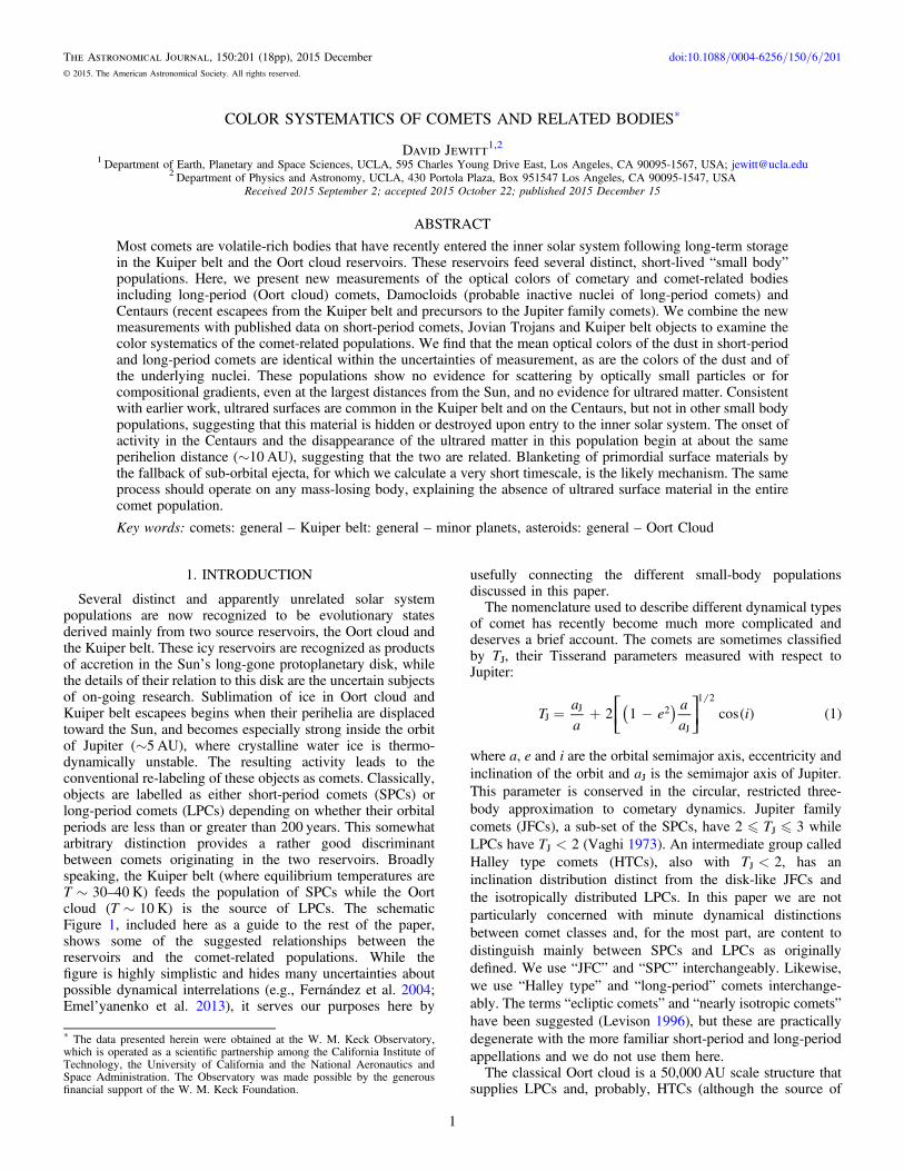
COLOR SYSTEMATICS OF COMETS AND RELATED BODIES*

David Jewitt1,21 Department of Earth, Planetary and Space Sciences, UCLA, 595 Charles Young Drive East, Los Angeles, CA 90095-1567, USA; [email protected]

2 Department of Physics and Astronomy, UCLA, 430 Portola Plaza, Box 951547 Los Angeles, CA 90095-1547, USAReceived 2015 September 2; accepted 2015 October 22; published 2015 December 15

ABSTRACT

Most comets are volatile-rich bodies that have recently entered the inner solar system following long-term storagein the Kuiper belt and the Oort cloud reservoirs. These reservoirs feed several distinct, short-lived “small body”populations. Here, we present new measurements of the optical colors of cometary and comet-related bodiesincluding long-period (Oort cloud) comets, Damocloids (probable inactive nuclei of long-period comets) andCentaurs (recent escapees from the Kuiper belt and precursors to the Jupiter family comets). We combine the newmeasurements with published data on short-period comets, Jovian Trojans and Kuiper belt objects to examine thecolor systematics of the comet-related populations. We find that the mean optical colors of the dust in short-periodand long-period comets are identical within the uncertainties of measurement, as are the colors of the dust and ofthe underlying nuclei. These populations show no evidence for scattering by optically small particles or forcompositional gradients, even at the largest distances from the Sun, and no evidence for ultrared matter. Consistentwith earlier work, ultrared surfaces are common in the Kuiper belt and on the Centaurs, but not in other small bodypopulations, suggesting that this material is hidden or destroyed upon entry to the inner solar system. The onset ofactivity in the Centaurs and the disappearance of the ultrared matter in this population begin at about the sameperihelion distance (∼10 AU), suggesting that the two are related. Blanketing of primordial surface materials bythe fallback of sub-orbital ejecta, for which we calculate a very short timescale, is the likely mechanism. The sameprocess should operate on any mass-losing body, explaining the absence of ultrared surface material in the entirecomet population.

Key words: comets: general – Kuiper belt: general – minor planets, asteroids: general – Oort Cloud

1. INTRODUCTION

Several distinct and apparently unrelated solar systempopulations are now recognized to be evolutionary statesderived mainly from two source reservoirs, the Oort cloud andthe Kuiper belt. These icy reservoirs are recognized as productsof accretion in the Sun’s long-gone protoplanetary disk, whilethe details of their relation to this disk are the uncertain subjectsof on-going research. Sublimation of ice in Oort cloud andKuiper belt escapees begins when their perihelia are displacedtoward the Sun, and becomes especially strong inside the orbitof Jupiter (∼5 AU), where crystalline water ice is thermo-dynamically unstable. The resulting activity leads to theconventional re-labeling of these objects as comets. Classically,objects are labelled as either short-period comets (SPCs) orlong-period comets (LPCs) depending on whether their orbitalperiods are less than or greater than 200 years. This somewhatarbitrary distinction provides a rather good discriminantbetween comets originating in the two reservoirs. Broadlyspeaking, the Kuiper belt (where equilibrium temperatures areT∼30–40 K) feeds the population of SPCs while the Oortcloud (T∼10 K) is the source of LPCs. The schematicFigure 1, included here as a guide to the rest of the paper,shows some of the suggested relationships between thereservoirs and the comet-related populations. While thefigure is highly simplistic and hides many uncertainties aboutpossible dynamical interrelations (e.g., Fernández et al. 2004;Emel’yanenko et al. 2013), it serves our purposes here by

usefully connecting the different small-body populationsdiscussed in this paper.The nomenclature used to describe different dynamical types

of comet has recently become much more complicated anddeserves a brief account. The comets are sometimes classifiedby TJ, their Tisserand parameters measured with respect toJupiter:

Taa

eaa

i2 1 cos 1JJ 2

J

1 2

( ) ( ) ( )= + -⎡⎣⎢

⎤⎦⎥

where a, e and i are the orbital semimajor axis, eccentricity andinclination of the orbit and aJ is the semimajor axis of Jupiter.This parameter is conserved in the circular, restricted three-body approximation to cometary dynamics. Jupiter familycomets (JFCs), a sub-set of the SPCs, have 2�TJ�3 whileLPCs have TJ<2 (Vaghi 1973). An intermediate group calledHalley type comets (HTCs), also with TJ<2, has aninclination distribution distinct from the disk-like JFCs andthe isotropically distributed LPCs. In this paper we are notparticularly concerned with minute dynamical distinctionsbetween comet classes and, for the most part, are content todistinguish mainly between SPCs and LPCs as originallydefined. We use “JFC” and “SPC” interchangeably. Likewise,we use “Halley type” and “long-period” comets interchange-ably. The terms “ecliptic comets” and “nearly isotropic comets”have been suggested (Levison 1996), but these are practicallydegenerate with the more familiar short-period and long-periodappellations and we do not use them here.The classical Oort cloud is a 50,000 AU scale structure that

supplies LPCs and, probably, HTCs (although the source of

The Astronomical Journal, 150:201 (18pp), 2015 December doi:10.1088/0004-6256/150/6/201© 2015. The American Astronomical Society. All rights reserved.

* The data presented herein were obtained at the W. M. Keck Observatory,which is operated as a scientific partnership among the California Institute ofTechnology, the University of California and the National Aeronautics andSpace Administration. The Observatory was made possible by the generousfinancial support of the W. M. Keck Foundation.

1

mailto:[email protected]

http://dx.doi.org/10.1088/0004-6256/150/6/201

HTCs has not been definitively established; c.f. Levisonet al. 2006; Emel’yanenko et al. 2013). Damocloids arepoint-like objects with TJ<2 that are likely to be the defunctnuclei of HTCs (Jewitt 2005), but again the details of thisconnection are not certain (Wang et al. 2012). Objects withperihelia between the orbits of Jupiter and Neptune are calledCentaurs. They are likely escaped Kuiper belt objects which, inturn, feed the population of JFCs. The Centaurs are short-lived(median lifetime ∼10Myr, albeit with a wide range; Horneret al. 2003, 2004; Tiscareno & Malhotra 2003) as a result ofstrong gravitational scattering interactions with the giantplanets. The JFCs are even shorter-lived (∼0.4 Myr; Levison& Duncan 1994) because of frequent scattering by theterrestrial planets. They also experience very rapid physicalevolution driven by sublimation. About 80% of the “asteroids”possessing JFC-like orbits have low, comet-like albedos (Kimet al. 2014).

Previous work has established that the Kuiper belt objectsdisplay an extraordinarily large range of optical colors (Luu &Jewitt 1996; Tegler & Romanishin 2000; Jewitt & Luu 2001;Hainaut & Delsanti 2002; Jewitt 2002; Tegler et al. 2003;Peixinho et al. 2004; Hainaut et al. 2012). This is due, in part,to the presence of ultrared matter which is defined as having anormalized reflectivity gradient S′�25% (1000Å)−1,

corresponding to optical colors B – R�1.6 mag (Jewitt2002). While irradiated organics have long been suspected tobe responsible for the red colors, the nature of the ultraredmatter remains unknown. We do know that the distribution ofultrared matter in the solar system is peculiar. It is mostconcentrated in the dynamically cold (low inclination) portionof the Classical Kuiper belt (Tegler & Romanishin 2000;Trujillo & Brown 2002) but is present in all the known Kuiperbelt populations (e.g., Sheppard 2010; Hainaut et al. 2012).Ultrared matter exists on the Centaurs, whose optical colordistribution appears to be bimodal (Peixinho et al. 2003, 2012;Tegler et al. 2003) but it has not been reported on other small-body populations (Jewitt 2002).In this paper, we present new optical measurements and

combine them with data from the literature in order to examinecolor systematics of the comet-related populations. We presentsystematic measurements of the LPCs, as a group, and the firstmeasurements of trans-Jovian LPCs (i.e., those with periheliabeyond Jupiter’s orbit, where sublimation of crystalline waterice is negligible). Our measurements of Damocloids andCentaurs extend earlier work (Jewitt 2005, 2009, respectively).The paper is divided as follows; Section 2 describes theobservational methods and object samples, Section 3 presentsresults that are discussed in Section 4, while Section 5 presentsa summary.

2. OBSERVATIONS

2.1. Methods

We used the 10 m diameter Keck I telescope located atopMauna Kea, Hawaii and the Low Resolution ImagingSpectrometer (LRIS) camera (Oke et al. 1995) to obtainphotometry. The LRIS camera has two channels housing redand blue optimized charge-coupled devices (CCDs) separatedby a dichroic filter (we used the “460” dichroic, which has 50%transmission at 4875Å). On the blue side we used a broadbandB filter (center wavelength λc = 4369Å, full width at halfmaximum (FWHM) Δλ = 880Å) and on the red side a V filter(λc = 5473Å, Δλ = 948Å) and an R filter (λc = 6417Å,Δλ = 1185Å). Some objects were also measured in the I filter(λc = 7600Å, Δλ = 1225Å). The I-filter measurements arelisted in the data-tables of this paper but have not been used inthe subsequent analysis because they are few in numbercompared to photometry in B, V and R. All observations usedthe facility atmospheric dispersion compensator to correct fordifferential refraction, and the telescope was tracked non-sidereally while autoguiding on fixed stars. The image scale onboth cameras was 0 135 pixel−1 and the useful field of viewapproximately 320″×440″. Atmospheric seeing ranged from∼0 7 to 1 3 FWHM and observations were taken only whenthe sky above Mauna Kea was photometric, as judged in real-time from a photometer at the nearby Canada–France–Hawaiitelescope and later by repeated measurements of photometricstandard stars.The data were reduced by subtracting a bias (zero exposure)

image and then dividing by a flat field image constructed fromintegrations taken on a diffusely illuminated spot on the insideof the Keck dome. The target objects were identified in theflattened images from their positions and distinctive non-sidereal motions. Photometry was obtained using circularprojected apertures tailored to the target and the individualnightly observing conditions, with sky subtraction obtained

Figure 1. Schematic flow diagram highlighting suspected connections betweencometary populations. Numbers give the approximate lifetimes of the differentstages. SPC—short-period comet, LPC—long period comet, HTC—Halley-type comet, dLPC and dJFC are defunct LPCs and JFCs, respectively. Severalsuggested connections (e.g., between the Scattered KBOs and the Oort cloud)have been omitted for clarity.

2

The Astronomical Journal, 150:201 (18pp), 2015 December Jewitt

from a contiguous annulus. In poor seeing we usedappropriately enlarged apertures. Observations of resolvedcomets generally used a sky annulus 12″ in radius and 6″ inwidth; the resulting contamination of the sky annulus bycometary dust is judged to be minimal. Photometric calibrationwas secured from observations of standard stars from Landolt(1992), always using the same apertures as employed for thetarget objects, on stars at similar airmass. We used only Landoltstars having ±0.01 mag or better uncertainties and colors closeto those of the Sun. Repeated measurements of the standardstars confirmed the photometric stability of each night at the∼±1% level.

The red-side CCD in LRIS is a physically thick device that isparticularly susceptible to “cosmic ray” (actually muon andother ionizing particles) contamination. We examined eachimage for such contamination and individually removedartifacts by digital interpolation before photometry wherepossible. In a few cases, long cosmic ray tracks (caused byenergetic particles grazing the CCD) could not be removed andwe eliminated these images from further consideration. Like-wise, objects whose photometry was contaminated by fieldstars and galaxies were revisited where possible, and ignoredfrom further consideration where not. Uncertainties wereestimated from the scatter of repeated measurements takenwithin a single night. Some objects were observed on morethan one night. In general, we find that the agreement betweennights is compatible with the photometric uncertaintiesestimated nightly.

2.2. The Observational Samples

The new measurements presented in this paper refer to thepopulations of LPCs, the Damocloids, and the Centaurs. Foreach of these populations we present the orbital properties, thegeometric circumstances of observation and the photometricresults in a series of data tables, as we shortly discuss. Theorbital properties are taken from the NASA JPL Horizonsephemeris service (http://ssd.jpl.nasa.gov/horizons.cgi),which was also used to compute the geometric circumstancesfor each observation. Photometric uncertainties on each object,σ, were computed from k d0

2 2 1 2( )s s= + , where σd is thestandard error on the mean of repeated measurements. Quantityk0 is a floor to the acceptable uncertainty estimated from thescatter in zero points deduced from observations of photometricstandard stars, and from inspection of real-time opacitymeasurements from the CFHT Skyprobe (http://www.cfht.hawaii.edu/Instruments/Elixir/skyprobe/home.html). Typi-cally, we found k0 = 0.01 while σd varied strongly with thebrightness of the object, as expected, and with the contaminat-ing effects of field stars and galaxies. The reported mean colorsof the different populations are given as unweighted means ofthe individual object colors, with the error on the meancomputed assuming Gaussian statistics (i.e., the error on themean is approximately the standard deviation of the populationdivided by the square root of the number of measurements). Weconservatively elected not to consider the weighted mean colorof a population because the weighting gives too much power tothe most precise photometry (typically of the brightest objects).However, in most cases, the unweighted mean and theweighted mean colors of a population are consistent.

Long Period Comets: We observed 26 LPCs (i.e., cometswith TJ<2), 18 of them with perihelion distance q>aJ,where aJ = 5.2 AU is the orbital semimajor axis of Jupiter.

Interest in the properties of these rarely observed trans-Jovianobjects is high, for two reasons. First, beyond Jupiter, the rateof sublimation of crystalline water ice is negligible, meaningthat any observed activity must have another cause (either thesublimation of a more volatile ice, or the action of a differentmechanism of ejection). Second, trans-Jovian radiation equili-brium temperatures are so low that ice grains expelled from thenucleus can survive in the coma, whereas the lifetimes of icegrains in the inner solar system are strongly curtailed bysublimation. Together, these effects (a potential change in thephysics of ejection and the preferential survival of volatilesolids at large distances) are expected to have observableeffects on the trans-Jovian LPCs.The orbital elements of the observed LPCs are listed in

Table 1. Two objects (2013 AZ60 with q = 7.9 AU and 2013LD16 with q = 2.545 AU) lack a cometary designation but areincluded in Table 1 because we have observed them to showcoma. Of the 18 trans-Jovian comets, three (namely C/2014 B1at q = 9.5 AU, C/2010 L3 at q = 9.9 AU and C/2003 A2 atq = 11.4 AU) have perihelia at or beyond the orbit of Saturn.Table 2 lists the geometric circumstances of observation for

each comet, while the color measurements are presented inTable 3. The mean colors of the LPCs from our observationsare B – V=0.78±0.02, V – R=0.47±0.02 and R – I=0.42±0.03. Some of the LPCs in our sample are likelymaking their first passage through the planetary system andmay show properties different from comets that have beenpreviously heated (for example, owing to the release of surfacematerial accumulated during 4.5 Gyr of exposure in the Oortcloud). To this end, we analyzed the pre-perihelion andpost-perihelion observations separately, finding B – V=0.81±0.02, V – R=0.47±0.02 and R – I=0.40±0.04(pre-perihelion) and B – V=0.75±0.02, V – R=0.47±0.02 and R – I=0.44±0.03 (post-perihelion), with 13 cometsin each group. No significant differences exist between the pre-and post-perihelion colors of the LPCs. Neither do the colorsshow a correlation with the orbital binding energy (taken as theinverse semi-major axis, from Table 1). We conclude that thereis no evidence for color differences that might be associatedwith the first entry of dynamically new comets into theplanetary region. This conclusion is tempered by intrinsicuncertainties in the orbits followed by comets in the past (e.g.,Królikowska & Dybczyński 2013).For comparison, the mean colors of six LPCs measured by

Solontoi et al. (2012) in the Sloan filter system (buttransformed to BVRI using the relations given by Ivezićet al. 2007) are B – V=0.76±0.01 (6), V – R=0.43±0.01,are in reasonable agreement with our data. The mean colorsof five LPCs reported by Meech et al. (2009) areB – V=0.687±0.005, V – R=0.443±0.003. While V – Ris again in good agreement, the latter B – V color appears bluerby ∼0.08 mag than in Solontoi et al. (2012) or the presentwork, and this difference is unexplained. Comet C/2003 A2,the only object observed in common between the Meechet al. paper and the present work, has consistent colors(V – R = 0.46±0.01, R – I = 0.39±0.01 from Meech et al.versus V – R = 0.47±0.04, R – I = 0.46±0.04 here) but wasnot measured in B – R. Object 2010 AZ60 was independentlyobserved by Pál et al. (2015), who found Sloan g′ – r′ =0.72±0.05. When transformed according to the prescriptionby Jester et al. (2005), this gives B – V=0.93±0.06.This compares with B – V=0.82±0.01 measured here. We

3


http://ssd.jpl.nasa.gov/horizons.cgi

http://www.cfht.hawaii.edu/Instruments/Elixir/skyprobe/home.html

http://www.cfht.hawaii.edu/Instruments/Elixir/skyprobe/home.html

consider this reasonable agreement given the large uncertaintieson the former measurement. Pal et al. did not comment on thecometary nature of 2010 AZ60.

Damocloids: The Damocloids are point-source objectshaving TJ<2, where TJ is the Tisserand parameter measuredwith respect to Jupiter (Jewitt 2005). The orbital elements ofthe Damocloids observed here are reported in Table 4 and thegeometric circumstances of observation may be found inTable 5. The measured colors of the Damocloids are listed inTable 6. The mean colors from these measurements alone areB – V=0.80±0.02, V – R=0.54±0.01, R – I=0.45±0.03 and B – R=1.34±0.02. Combined with additionalmeasurements from Table 4 of Jewitt (2005), we obtainmean colors B – V=0.80±0.02, V – R=0.51±0.02,R – I= 0.47±0.02 and B – R=1.31±0.02.

Two of the 15 observed Damocloids, C/2010 DG56 and C/2014 AA52, received cometary designations between theirselection for this study and their observation at the Keck. Athird, 2013 LD16, was found by us to be cometary, although itretains an asteroidal designation. This transformation frominactive to active also occurred in our original study ofthe Damocloids (Jewitt 2005), and provides strong evidencethat bodies selected as probable defunct comets on the basisof their distinctive orbits indeed carry near-surface volatiles. Wemoved the active Damocloids to our LPC sample. The colors ofobject 342842 (2008 YB3) were independently measured by

Sheppard (2010) as B – R=1.26±0.01, V – R=0.46±0.01,and by Pinilla-Alonso et al. (2013) as B – R=1.32±0.06,V – R=0.50±0.06, in reasonable agreement with the colorsmeasured here B – R= 1.25±0.02, V – R=0.51±0.02.Centaurs: To define our Centaur sample (Table 7), we

selected objects having perihelia q>aJ and semimajor axesa aN∣ ∣ < , ignoring objects in 1:1 resonance with the giantplanets (c.f. Jewitt 2009). This is a narrower definition than isemployed by some dynamicists, but serves to provide aconvenient sample distinct from the Kuiper belt objects atlarger semimajor axes and the SPCs at smaller distances. Weobserved 17 Centaurs, 7 of them active. The geometriccircumstances of observation are given in Table 8 while thephotometry is given in Table 9. To the new observations inthese tables we add separate measurements of the colors ofCentaurs using data from Jewitt (2009) and from Peixinho et al.(2003) and Peixinho et al. (2012). We consider the inactive andactive Centaurs separately. Their colors appear quite differentin being, for the inactive Centaurs B – V=0.93±0.04 (29),V – R=0.55±0.03 (29), R – I=0.45±0.02(3) and forthe active objects B – V=0.80±0.03 (12), V – R=0.50±0.03 (13).Active SPCs: We used results from a survey by Solontoi

et al. (2012), who found mean colors B – V=0.80±0.01(20), V – R=0.46±0.01 (20). These measurements weretaken using the SLOAN broadband filter system and

Table 1Long Period Comet Orbital Elements

N Object qa ab ec id TPe

1 C/2003 A2 (Gleason) 11.427 −1643.9 1.007 8.1 2003 Nov 04.02 C/2004 D1 (NEAT) 4.975 −3056.1 1.002 45.5 2006 Feb 10/83 C/2006 S3 (Loneos) 5.131 −1672 1.0031 166.0 2012 Apr 16.54 C/2007 D1 (LINEAR) 8.793 −30938 1.000 41.5 2007 Jun 19.05 C/2008 S3 (Boattini) 8.019 −7505.6 1.001 162.7 2011 Jun 05.96 C/2009 T1 (McNaught) 6.220 3837.1 0.998 89.9 2009 Oct 08.27 C/2010 D4 (WISE) 7.148 64.656 0.889 105.7 2009 Mar 30.98 C/2010 DG56 (WISE) 1.591 67.525 0.976 160.4 2010 May 15.69 C/2010 L3 (Catalina) 9.882 12180.5 0.999 102.6 2010 Nov 10.410 C/2010 U3 (Boattini) 8.469 −7071.7 1.001 55.42 2019 Feb 26.311 C/2011 Q1 (PANSTARRS) 6.780 3285.0 0.998 94.9 2011 Jun 29.412 C/2012 A1 (PANSTARRS) 7.605 −7505.85 1.001 120.9 2013 Nov 29.313 C/2012 E1 (Hill) 7.503 3761.43 0.998 122.5 2011 Jul 04.014 C/2012 K8 (Lemmon) 6.464 −2021.4 1.003 106.1 2014 Aug 19.215 C/2012 LP26 (Palomar) 6.534 3954.3 0.998 25.4 2015 Aug 17.516 2013 AZ60 7.911 991.67 0.992 16.5 2014 Nov 22.217 C/2013 E1 (McNaught) 7.782 −3133.88 1.003 158.7 2013 Jun 12.118 C/2013 H2 (Boattini) 7.499 −2657.52 1.003 128.4 2014 Jan 23.219 2013 LD16 2.545 80.008 0.968 154.7 2013 Oct 14.820 C/2013 P3 (Palomar) 8.646 9.99e99 1. 93.9 2014 Nov 24.121 C/2014 AA52 (CATALINA) 2.003 −5503.2 1.000 105.2 2015 Feb 27.622 C/2014 B1 (Schwarz) 9.531 −642.7 1.015 28.4 2017 Sep 06.323 C/2014 R1 (Borisov) 1.345 181.9 0.993 9.9 2014 Nov 19.224 C/2014 W6 (Catalina) 3.088 −1659 1.0019 53.6 2015 Mar 19.025 C/2014 XB8 (PANSTARRS) 3.011 1902749 0.999998 149.8 2015 Apr 05.526 C/2015 B1 (PANSTARRS 3.700 9.99e99 1. 20.8 2016 Sep 20.9

Notes.a Perihelion distance, AU.b Orbital semimajor axis, AU.c Orbital eccentricity.d Orbital inclination, degree.e Date of perihelion.

4


transformed to BVR. The transformation may incur a smalluncertainty, probably of order 0.01 mag, in addition to thequoted statistical uncertainty.

Active Cometary Nuclei: The colors of cometary nuclei havebeen reported in Tables 3 and 5 of the compilation by Lamy &Toth (2009). The accuracy of many of these colors depends ondigital processing to remove near-nucleus coma and severaldiscrepant or anomalous objects exist. We reject objects (forexample, 6P/d’Arrest) having wildly inconsistent colors, andobjects for which the B – R color is uncertain by σ>0.1 mag.The resulting sample has 16 SPC nuclei (2�TJ�3), forwhich the mean colors and the standard errors on the means areB – V=0.87±0.05, V – R=0.50±0.03, R – I=0.46±0.03, giving B – R=1.37±0.08.

The sample also includes five comets with TJ<2, (i.e., LPCnuclei) for which the mean colors are B – V=0.77±0.02,V – R=0.44±0.02, R – I=0.44±0.02(5) and B – R=1.22± 0.03.

Defunct Short-period Nuclei: The colors of the defunctnuclei of SPCs, sometimes called ACOs (Asteroids inCometary Orbits), have been measured by several authors.Alvarez-Candal (2013) found a mean reflectivity gradientS′ = 2.8% (1000Å)−1 (no uncertainty quoted) from a sample

of 94 objects, after eliminating 73 objects “with behaviorsimilar to S- or V- type asteroids,” leading to a value that islikely artificially blue. Licandro et al. (2008) reported spectra of57 objects and from them derived S′ = 4.0% (1000Å)−1 (againwith no quoted uncertainty). The latter value of S′ wouldcorrespond approximately to broadband colors B – V=0.68,V – R=0.39. However, both studies note that there is a trendfor the colors to become more red as the Tisserand parameterdecreases, consistent with dynamical inferences that the“comet-like orbits” are fed from a mix of cometary andasteroid-belt sources.Jupiter Trojans: The Jovian Trojans have no known

association with the Kuiper belt or Oort cloud comet reservoirsbut we include them for reference because some models posit anorigin by capture from the Kuiper belt (Nesvorný et al. 2013).We take the mean colors of Jovian Trojans from a large study bySzabó et al. (2007), who reported B – V=0.73±0.08,V – R=0.45±0.08, R – I=0.43± 0.10 (where the quoteduncertainties are the standard deviations, not the errors on themeans). The Szabo et al. sample is very large (N∼300) and, asa result, the standard errors on the mean colors are unphysicallysmall. We set the errors on the mean colors equal to ±0.02magto reflect the likely presence of systematic errors of this order.

Table 2Long Period Comet Observational Geometry

N Object UT Date rHa Δb αc

1 C/2003 A2 (Gleason) 2005 Jan 15 11.640 10.921 3.42 C/2004 D1 (NEAT) 2005 Jan 15 5.799 5.041 9.03 C/2006 S3 (Loneos) 2015 Feb 18 9.011 8.164 3.44 C/2007 D1 (LINEAR) 2010 Mar 17 10.490 9.587 2.45 C/2008 S3 (Boattini) 2010 Aug 10 8.222 8.055 7.0

” 2010 Sep 10 8.182 7.505 5.56 C/2009 T1 (McNaught) 2011 Jan 30 7.024 6.894 8.07 C/2010 D4 (WISE) 2010 Sep 10 7.822 8.114 6.98 C/2010 DG56 (WISE) 2010 Sep 10 2.210 1.226 7.39 C/2010 L3 (Catalina) 2010 Sep 10 9.889 10.094 5.710 C/2010 U3 (Boattini) 2011 Jan 30 17.982 18.003 3.1

” 2012 Oct 13 15.382 14.487 1.7” 2012 Oct 14 15.378 14.487 1.6

11 C/2011 Q1 (PANSTARRS) 2012 Oct 13 7.449 6.961 6.9” 2012 Oct 14 7.452 6.998 7.0

12 C/2012 A1 (PANSTARRS) 2014 Feb 26 7.621 7.333 7.313 C/2012 E1 (Hill) 2014 Feb 26 9.567 9.048 5.214 C/2012 K8 (Lemmon) 2012 Oct 13 7.872 7.695 7.215 C/2012 LP26 (Palomar) 2012 Oct 13 9.378 10.174 3.5

” 2012 Oct 14 9.374 10.176 3.5” 2014 Feb 27 7.442 7.677 7.3

16 2013 AZ60 2014 Feb 26 8.077 7.214 3.617 C/2013 E1 (McNaught) 2014 Feb 26 7.944 6.983 1.818 C/2013 H2 (Boattini) 2014 Feb 27 7.502 7.384 7.619 2013 LD16d 2014 Feb 27 2.915 2.001 9.120 C/2013 P3 (Palomar) 2013 Oct 01 8.984 8.101 3.221 C/2014 AA52 (CATALINA) 2014 Feb 26 4.483 3.563 5.222 C/2014 B1 (Schwarz) 2014 Feb 26 11.875 11.462 4.423 C/2014 R1 (Borisov) 2015 Feb 18 1.875 1.882 30.524 C/2014 W6 (Catalina) 2015 Feb 18 3.100 2.282 12.025 C/2014 XB8 (PANSTARRS) 2015 Feb 17 3.047 3.239 17.826 C/2015 B1 (PANSTARRS) 2015 Feb 18 6.145 5.203 3.0

Notes.a Heliocentric distance, AU.b Geocentric distance, AU.c Phase angle, degree.

5


Independent colors determined from a much smaller sample(N = 29), B – V= 0.78±0.09, V – R=0.45±0.05,R – I=0.40±0.10 arein agreement with the values by Szabo et al. (Fornasieret al. 2007).

Kuiper Belt Objects: The colors of Kuiper belt objects aredistinguished by their extraordinary range (Luu & Jewitt 1996),and by the inclusion of some of the reddest material in the solarsystem (Jewitt 2002). Their colors have been compiled innumerous sources (e.g., Hainaut & Delsanti 2002; Hainautet al. 2012). Here, we use the online compilation provided byTegler, http://www.physics.nau.edu/~tegler/research/survey.htm, which is updated from a series of publications (most fromTegler & Romanishin 2000; Tegler et al. 2003) and has theadvantages of uniformity and high quality. Note that the colorsof Kuiper belt objects are employed only to provide context tothe new measurements, and our conclusions would not bematerially changed by the use of another Kuiper belt dataset.The mean colors of Kuiper belt objects are B – V = 0.92 ±0.02, V – R = 0.57 ± 0.02. It is well known that the KBOcolors are diverse, and so we additionally compute colors for

dynamical sub-groups (the hot and cold Classical KBOs, the3:2 resonant Plutinos and the scattered KBOs), again usingmeasurements from Tegler et al. for uniformity.

3. RESULTS

The color data are summarized in Table 10 where, for eachcolor index and object type, we list the median color and themean value together with the error on the mean and, inparentheses, the number of objects used. We note an agreeableconcordance between the median and mean colors of mostobject classes, showing that the color distributions are nothighly skewed (the main exception is found in the B – R colorof the inactive Centaurs, with median and mean colors differingby nearly three times the error on the mean). We note that thelisted uncertainties are typically ±0.02 mag and larger, and thateven the B – V color of the Sun has an uncertainty of 0.02 mag(Holmberg et al. 2006).We are first interested to know if the measured colors of

the LPCs might be influenced by the angular sizes of theapertures used to extract photometry. If so, the colors ofobjects measured using fixed angle apertures might appear

Table 3Long Period Comet Photometry

N Object UT Date Notea fb mRc B − V V − R R − I B − R

1 C/2003 A2 (Gleason) 2005 Jan 15 E 6.0 19.96±0.03 0.61±0.04 0.47±0.04 0.46±0.04 1.08±0.042 C/2004 D1 (NEAT) 2005 Jan 15 E 6.0 17.54±0.03 0.82±0.05 0.43±0.04 0.51±0.04 1.25±0.053 C/2006 S3 (Loneos) 2015 Feb 18 E 8.1 17.57±0.01 0.74±0.01 0.58±0.01 K 1.32±0.024 C/2007 D1 (LINEAR) 2010 Mar 17 E 5.4 18.85±0.02 0.75±0.02 0.44±0.02 0.41±0.03 1.19±0.035 C/2008 S3 (Boattini) 2010 Aug 10 E 6.8 18.57±0.02 0.74±0.05 0.48±0.04 0.38±0.04 1.22±0.05

” 2010 Sep 10 E 8.2 18.23±0.01 0.78±0.02 0.44±0.01 0.36±0.01 1.22±0.026 C/2009 T1 (McNaught) 2011 Jan 30 E 9.4 19.25±0.03 0.64±0.04 0.53±0.03 0.45±0.03 1.17±0.037 C/2010 D4 (WISE) 2010 Sep 10 P 8.0 20.91±0.05 0.74±0.07 0.46±0.05 K 1.20±0.058 C/2010 DG56 (WISE) 2010 Sep 10 E 8.0 19.98±0.03 0.77±0.05 0.37±0.05 K 1.14±0.059 C/2010 L3 (Catalina) 2010 Sep 10 E 5.6 19.94±0.02 0.75±0.03 0.42±0.03 0.41±0.03 1.17±0.0310 C/2010 U3 (Boattini) 2011 Jan 30 E 9.4 20.09±0.05 0.82±0.05 0.48±0.04 0.32±0.05 1.30±0.06

” 2012 Oct 13 E 6.8 20.04±0.02 0.81±0.03 0.54±0.03 K 1.35±0.03” 2012 Oct 14 E 6.8 19.86±0.02 0.72±0.03 0.53±0.03 K 1.25±0.03

11 C/2011 Q1 (PANSTARRS) 2012 Oct 13 E 6.8 20.98±0.06 0.83±0.05 0.51±0.07 K 1.34±0.07” 2012 Oct 14 E 6.8 21.02±0.02 0.81±0.04 0.48±0.03 K 1.29±0.04

12 C/2012 A1 (PANSTARRS) 2014 Feb 26 E 8.0 18.84±0.02 0.74±0.01 0.45±0.02 K 1.19±0.0313 C/2012 E1 (Hill) 2014 Feb 26 E 8.1 21.84±0.05 0.79±0.09 0.40±0.07 K 1.19±0.0914 C/2012 K8 (Lemmon) 2012 Oct 13 P 6.8 K 0.72±0.01 K K K15 C/2012 LP26 (Palomar) 2012 Oct 13 E 6.8 19.60±0.03 0.88±0.03 0.52±0.04 K 1.40±0.04

” 2012 Oct 14 E 6.8 19.57±0.01 0.91±0.02 0.58±0.01 K 1.49±0.01” 2014 Feb 27 E 8.1 19.12±0.01 0.78±0.02 0.45±0.01 K 1.23±0.02

16 2013 AZ60 2014 Feb 26 E 8.1 18.85±0.01 0.82±0.01 0.54±0.01 K 1.36±0.0117 C/2013 E1 (McNaught) 2014 Feb 26 E 8.1 19.16±0.02 0.75±0.03 0.48±0.03 K 1.23±0.0318 C/2013 H2 (Boattini) 2014 Feb 27 E 8.1 18.80±0.01 0.77±0.02 0.49±0.01 K 1.26±0.0219 2013 LD16 2014 Feb 27 E 8.0 20.15±0.02 0.86±0.05 0.44±0.03 K 1.30±0.0220 C/2013 P3 (Palomar) 2013 Oct 01 E 8.1 19.78±0.04 0.92±0.05 0.45±0.05 K 1.37±0.0621 C/2014 AA52 (CATALINA) 2014 Feb 26 E 8.0 18.36±0.02 0.77±0.02 0.41±0.02 K 1.18±0.0322 C/2014 B1 (Schwarz) 2014 Feb 26 E 8.1 19.20±0.02 0.85±0.03 0.58±0.03 K 1.43±0.0323 C/2014 R1 (Borisov) 2015 Feb 18 E 8.1 15.40±0.01 0.81±0.01 0.46±0.01 K 1.27±0.0124 C/2014 W6 (Catalina) 2015 Feb 18 E 8.1 18.09±0.01 0.81±0.01 0.45±0.01 K 1.26±0.0125 C/2014 XB8 (PANSTARRS) 2015 Feb 17 E 5.4 20.92±0.02 0.79±0.03 0.44±0.03 K 1.23±0.0326 C/2015 B1 (PANSTARRS) 2015 Feb 18 E 8.1 19.51±0.01 0.78±0.01 0.45±0.01 K 1.23±0.01

Sund K K K K 0.64±0.02 0.35±0.01 0.33±0.01 0.99±0.02

Notes.a Morphology; P = point source, E = extended.b Angular diameter of photometry aperture in arcsecond.c Apparent red magnitude inside aperture of diameter f.d Holmberg et al. (2006).

6


http://www.physics.nau.edu/~tegler/research/survey.htm

http://www.physics.nau.edu/~tegler/research/survey.htm

to depend on geocentric distance. Color gradients areexpected if, for example, the nuclei and the dust coma of agiven object have intrinsically different colors, or if theparticles properties change with time since release from thenucleus. In almost every comet observed here, inspection ofthe surface brightness profiles shows that the cross-section inthe photometry aperture is dominated by dust, not by thegeometric cross-section of the central nucleus. We also notethat spectra of distant comets are invariably continuumdominated (indeed, gaseous emission lines are usually noteven detected, e.g., Ivanova et al. 2015) because of the stronginverse distance dependence of the resonance-fluorescenceline strength.

We compare measurements of active comets using apertureshaving different angular radii in Table 11 and show themgraphically in Figure 2. To maximize the color differences andshow the results most clearly, we consider only the B – R colorindex. The data show that real color variations with angular

radius do exist in some active comets but that these variationsare small, never larger than 0.1 mag in B – R over the range ofradii sampled and more typically only a few ×0.01 mag.Moreover, the color gradients with angular radius can bepositive (as in C/2006 S3) or negative (e.g., C/2014 XB8).These findings are consistent with measurements reportedfor five active Centaurs (Jewitt 2009). For the comets inFigure 2, radial color variations are likely to result fromsmall changes in the particle properties as a function of thetime since release from the nucleus. For example, dustfragmentation and/or the loss of embedded volatiles couldcause color gradients across the comae. Here, we merely notethe possible existence of these effects and remark on theirevident small size. There is no evidence from the measuredcomets that the comae are systematically different from thecentral nuclei.Figure 3 shows B – R of the comets as a function of the

heliocentric distance, rH, including data from Solontoi et al.(2012) for comets inside Jupiter’s orbit. The figure shows noevidence for a trend, consistent with Jewitt & Meech (1988),Solontoi et al. (2012) but over a much larger range ofheliocentric distances (∼1 to ∼12 AU) that straddles the waterice sublimation zone near 5–6 AU.Figure 4 shows the B – R color of the comets as a function of

the perihelion distance, q. Clearly, there is no discerniblerelation between B – R and q. This is significant because, asnoted above, the mechanism for mass loss likely changes withincreasing distance from the Sun. Comets active beyond theorbit of Jupiter are likely to be activated by the sublimation ofices more volatile than water and/or by different processes (forexample, the exothermic crystallization of ice). The meancolors of the active SPCs and LPCs are indistinguishable in thefigure, mirroring the absence of significant compositionaldifferences between these two groups in measurements ofgas-phase species (A’Hearn et al. 2012).The LPC colors are compared with the colors of Kuiper belt

objects in Figure 5. The color of the Sun (Holmberg et al. 2006)is shown as a yellow circle. While both sets of objects fall onthe same color–color line, the comets show no evidence forredder colors (B – R�1.50, B – V�0.95) that are commonlyfound in members of the Kuiper belt. Figure 5 shows that theLPCs are devoid of the ultrared matter. The significance of the

Table 4Damocloid Orbital Elements


1 2010 BK118 6.106 452.642 0.987 143.9 2012 Apr 30.22 2010 OM101 2.129 26.403 0.919 118.7 2010 Oct 01.43 2010 OR1 2.052 27.272 0.925 143.9 2010 Jul 12.54 2012 YO6 3.304 6.339 0.479 106.9 2012 Jul 30.35 2013 NS11 2.700 12.646 0.786 130.4 2014 Sep 26.26 2013 YG48 2.024 8.189 0.753 61.3 2014 Mar 11.67 2014 CW14 4.235 19.810 0.786 170.6 2014 Dec 23.48 330759 (2008 SO218) 3.546 8.148 0.565 170.4 2009 Dec 31.29 336756 (2010 NV1) 9.417 292.030 0.968 140.8 2010 Dec 13.210 342842 (2008 YB3) 6.487 11.651 0.443 105.0 2011 Mar 01.711 418993 (2009 MS9) 11.004 387.251 0.972 68.0 2013 Feb 11.7

a Perihelion distance, AU.b Orbital semimajor axis, AU.c Orbital eccentricity.d Orbital inclination, degree.e Date of perihelion.

Table 5Damocloid Observational Geometry


1 2010 BK118 2011 Jan 30 6.855 7.079 7.9” 2010 Sep 10 7.330 6.825 7.1

2 2010 OM101 2010 Aug 10 2.208 1.780 26.8” 2010 Sep 10 2.143 1.469 24.4

3 2010 OR1 2010 Aug 10 2.079 1.278 22.0” 2010 Sep 10 2.164 1.254 15.1

4 2012 YO6 2013 Oct 01 4.243 3.938 13.45 2013 NS11 2014 Feb 26 3.312 2.813 16.16 2013 YG48 2014 Feb 26 2.028 1.268 22.8

” 2014 Feb 27 2.028 1.278 23.27 2014 CW14 2014 Feb 26 4.770 3.845 4.78 330759 (2008 SO218) 2010 Sep 10 3.937 3.197 11.09 336756 (2010 NV1) 2010 Aug 10 9.441 8.851 5.210 342842 (2008 YB3) 2014 Feb 26 7.998 7.609 6.711 418993 (2009 MS9) 2010 Sep 10 11.886 11.553 4.6


7


difference is self-evident from the figure. It can be simplyquantified by noting that none of the 26 measured LPCs hascolors redder than the median color of cold classical KBOs.The probability of finding this asymmetric distribution bychance is (1/2)26∼10−8, by the definition of the median. TheKolmogorov–Smirnov (KS) test applied to the color datashows that the likelihood that the B – R distributions of theLPCs and KBOs are drawn from the same parent distribution is<0.001, confirming a >3σ difference.

The colors of the inactive (point-source) Centaurs (bluecircles) are plotted with their formal uncertainties in Figure 6,where they are compared with the color distribution ofthe Kuiper belt objects (gray circles) taken from Tegler. Themean colors of the inactive Centaurs are B – V=0.93±0.04(29), V – R=0.55±0.03 (29) and B – R=1.47±0.06(N = 32), overlapping the mean colors of the KBOs(B – V = 0.91±0.02, V – R = 0.57±0.01 and B – R =1.48±0.03). Not only do the mean colors agree, but

Table 6Damocloid Photometry


1 2010 BK118 2011 Jan 30 P 5.4 18.97±0.02 0.76±0.03 0.57±0.03 0.51±0.03 1.33±0.03” 2010 Sep 10 P 8.0 20.06±0.02 0.80±0.02 0.52±0.02 0.45±0.03 1.32±0.03

2 2010 OM101 2010 Aug 10 P 5.6 20.64±0.03 0.81±0.04 0.53±0.04 K 1.34±0.05” 2010 Sep 10 P 5.6 19.94±0.07 0.77±0.07 0.69±0.07 0.36±0.07 1.46±0.07

3 2010 OR1 2010 Aug 10 P 6.8 18.94±0.02 0.76±0.03 0.52±0.02 0.48±0.04 1.28±0.04” 2010 Sep 10 P 8.0 19.97±0.02 0.81±0.04 0.51±0.04 0.43±0.02 1.32±0.03

4 2012 Y06 2013 Oct 01 P 8.0 21.59±0.05 K K 0.34±0.05 1.32±0.055 2013 NS11 2014 Feb 26 P 8.0 19.12±0.03 0.74±0.02 0.56±0.04 K 1.30±0.036 2013 YG48 2014 Feb 26 P 8.0 20.13±0.02 0.77±0.02 0.55±0.02 K 1.32±0.02

” 2014 Feb 27 P 5.4 19.94±0.01 0.83±0.02 0.48±0.02 K 1.31±0.027 2014 CW14 2014 Feb 26 P 8.0 20.97±0.02 0.87±0.09 0.51±0.06 K 1.38±0.078 330759 (2008 SO218) 2010 Sep 10 P 5.6 18.81±0.01 0.89±0.03 0.55±0.02 0.50±0.04 1.44±0.029 336756 (2010 NV1) 2010 Aug 10 P 8.0 20.31±0.02 0.79±0.03 0.53±0.03 0.39±0.02 1.32±0.0310 342842 (2008 YB3) 2014 Feb 26 P 8.0 18.35±0.01 0.74±0.02 0.51±0.02 K 1.25±0.0211 418993 (2009 MS9) 2010 Sep 10 P 3.8 20.79±0.04 0.84±0.04 0.52±0.04 K 1.36±0.04

Sund K K K K 0.64±0.02 0.35±0.01 0.33±0.01 0.99±0.02

Notes.a Morphology; P = point source, E = extended.b Angular diameter of photometry aperture in arcsecond.c Apparent red magnitude measured in aperture of diameter f.d Holmberg et al. (2006).

Table 7Centaur Orbital Elements


1 2001 XZ255 15.476 16.026 0.034 2.6 1986 May 06.92 2010 BL4 8.573 18.534 0.537 20.8 2009 Jul 27.13 2010 WG9 18.763 53.729 0.651 70.2 2006 Feb 20.44 2013 BL76 8.374 1216.0 0.993 98.6 2012 Oct 27.75 2014 HY123 6.998 18.552 0.623 14.0 2017 Jan 08.16 2015 CM3 6.784 13.182 0.485 19.7 2013 Apr 26.07 32532 Thereus (2001 PT13) 8.513 10.615 0.198 20.4 1999 Feb 12.08 148975 (2001 XA255) 9.338 29.617 0.685 12.6 2010 Jun 19.29 160427 (2005 RL43) 23.449 24.550 0.045 12.3 1991 Sep 13.610 433873 (2015 BQ311) 5.051 7.140 0.293 24.5 2007 Oct 16.111 C/2011 P2 (PANSTARRS) 6.148 9.756 0.370 9.0 2010 Sep 13.512 P/2011 S1 (Gibbs) 6.897 8.655 0.203 2.7 2014 Aug 20.213 C/2012 Q1 (Kowalski) 9.482 26.154 0.637 45.2 2012 Feb 09.414 C/2013 C2 (Tenagra) 9.132 15.993 0.429 21.3 2015 Aug 28.615 C/2013 P4 (PANSTARRS) 5.967 14.779 0.596 4.3 2014 Aug 12.416 166P/NEAT 8.564 13.883 0.383 15.4 2002 May 20.817 167P/CINEOS 11.784 16.141 0.270 19.1 2001 Apr 10.0

Notes.a Perihelion distance, AU.b Orbital semimajor axis, AU.c Orbital eccentricity.d Orbital inclination, degree.e Epoch of perihelion.

8


Figure 6 shows that the inactive Centaurs and the KBOs spanthe same large range of colors. The inactive Centaurs, however,show B – V, V – R colors that are bimodally clustered towardthe ends of the color distribution defined by the KBOs, withfew examples near the mean color of the KBOs. Thisbimodality was noted by Peixinho et al. (2003), Tegler et al.(2003) and Peixinho et al. (2012), and is an unexplained butapparently real feature of the Centaur color distribution. Itindicates that there are two surface types with few intermediateexamples.

By comparison, the mean colors of the active Centaurs areless red, with B – V=0.80±0.03, V – R=0.50±0.03,B – R=1.30±0.05, while comparison of Figures 6 and 7shows that the distribution of the colors is qualitativelydifferent from that of the inactive Centaurs. The activeCentaur distribution is unimodal, with most of the activeCentaurs being less red than the average color of the KBOs.The B – R color distributions are compared as a histogramin Figure 8.

We estimate the statistical significance of the differencebetween the active Centaurs and the KBOs using the non-parametric KS test to compare B – R. Based on this test,the likelihood that the two populations could be drawn bychance from a single parent population is ∼6%. In a Gaussiandistribution, this would correspond roughly to a 2σ (95%)difference. Thus, while Figure 7 is suggestive, we cannotyet formally conclude at the 3σ level of confidence thatthe active and inactive Centaurs have different colordistributions.

Figure 9 shows the Damocloids on the Kuiper belt color fieldplot. The new data confirm the absence of ultrared matterpreviously noted in the Damocloid population (c.f. Jewitt 2005)but in a sample that is twice as large.

4. DISCUSSION

The summary data from Table 10 are plotted in Figure 10.Also plotted for reference in Figure 10 are the colors ofcommon asteroid spectral types, tabulated by Dandy et al.(2003). The solid line in color–color plot Figure 10 is thereddening line for objects having linear reflectivity gradients,S′=dS/dλ = constant, where S is the normalized ratio of theobject brightness to the solar brightness (Jewitt & Meech 1988).Numbers along the line show the magnitude of S′, in units of %(1000Å)−1. Deviations from the line indicate spectral curva-ture, with objects below the line having concave reflectionspectra across the B to R wavelengths (d2S/dλ2>0) whilethose above it are convex (d2S/dλ2<0). The figure showsthat, whereas the reflection spectra of many common asteroidtypes are concave in the B – R region (as a result of broadabsorption bands), the comet-related populations all fall closeto the reddening line, consistent with having linear reflectivityspectra. We emphasize that the reddening line has zero freeparameters and is not a fit to the data. That the mean colormeasurements fall within a few hundredths of a magnitudefrom the reddening line gives us confidence that theuncertainties (which are on the same order) have been correctlyestimated. However, it is important to remember that these arethe average colors of each group, and that individual objectscan have colors and spectral curvatures widely different fromthe average values.The comet-related populations, including the active comets

themselves, are systematically redder than the C-complexasteroids (C, B, F, G) that are abundant members of the outerasteroid belt. The Jovian Trojans, the least-red of the plottedobjects, have mean optical colors that are identical to those ofthe D-type asteroids within the uncertainties of measurement.The most red objects in Figure 10 are the low-inclination(i�2°) Classical KBOs.

4.1. The Absence of Blue Scattering in Cometary Dust

We find no significant difference between the mean opticalcolors of dust in short-period (Kuiper belt) and long-period(Oort cloud) comets. Comparable uniformity is observed in thegas phase compositions of comets, where significant abundancedifferences exist but are uncorrelated with the dynamical type(Cochran et al. 2015). In both dust and gas, relative uniformityof the properties is consistent with radial mixing of the sourcematerials in the protoplanetary disk, and with population of theKuiper belt and Oort cloud from overlapping regions ofthis disk.We expect that the colors of cometary dust should become

more blue with increasing heliocentric distance, for tworeasons. First, the size of the largest particle that can beaccelerated to the nucleus escape velocity is a strong functionof the gas flow and hence of the heliocentric distance. At largedistances the mean size of the ejected particles should fall intothe optically small regime (defined for a sphere of radius a byx<1, where x=2πa/λ is the ratio of the particle circumfer-ence to the wavelength of observation), leading to non-geometric scattering effects that include anomalous (blue)colors (Bohren & Huffman 1983; Brown 2014). Second, icegrains have been detected spectrally in comets (e.g., Kawakitaet al. 2004; Yang et al. 2009, 2014) and should be moreabundant in distant comets as a result of their lowertemperatures, reduced sublimation rates and longer lifetimes.

Table 8Centaur Observational Geometry


1 2001 XZ255 2003 Jan 09 16.079 15.096 0.12 2010 BL4 2010

Mar 178.632 8.017 5.4

3 2010 WG9 2011 Jan 29 19.621 19.161 2.64 2013 BL76 2013 Oct 01 8.610 7.627 1.35 2014 HY123 2015 Feb 17 7.818 6.838 1.06 2015 CM3 2015 Feb 17 7.417 6.540 3.77 32532 Thereus (2001 PT13) 2007 Feb 20 10.792 11.233 4.6

” 2015 Feb 17 12.703 12.087 3.68 148975 (2001 XA255) 2003 Jan 09 14.965 13.982 0.19 160427 (2005 RL43) 2014 Feb 26 24.142 24.544 2.110 433873 (2015 BQ311) 2015 Feb 17 8.888 7.944 2.011 C/2011 P2 (PANSTARRS) 2014 Oct 22 8.412 7.475 2.412 P/2011 S1 (Gibbs) 2014 Feb 26 6.914 7.398 6.913 C/2012 Q1 (Kowalski) 2012 Oct 13 9.546 8.837 4.4

” 2012 Oct 14 9.546 8.848 4.4” 2013 Oct 01 9.849 8.903 2.0

14 C/2013 C2 (Tenagra) 2014 Feb 26 9.355 8.478 3.015 C/2013 P4 (PANSTARRS) 2014 Oct 22 5.980 5.015 2.516 166P/NEAT 2015 Feb 17 15.640 14.700 1.117 167P/CINEOS 2010 Sep 10 14.415 13.481 1.6

” 2012 Oct 13 15.332 14.398 1.3


9


Pure ice grains are bluer than more refractory silicate andcarbonaceous solids and thus the average color should againbecome more blue with increasing distance from the Sun.Indeed, Hartmann & Cruikshank (1984) reported a color-distance gradient in comets but this has not been independentlyconfirmed (Jewitt & Meech 1988; Solontoi et al. 2012) and isabsent in the present work (Figure 3). While one might expectthat the dust in distant comets should begin to show blue colorsconsistent with small-particle scattering and with an increasingice fraction, this is not observed. We briefly discuss why thismight be so.

With λ = 0.5 μm, x∼1 corresponds to particle radiiac∼0.1 μm. Larger particles scatter in proportion to theirphysical cross-section while in smaller particles the scatteringcross-section also depends on the wavelength. The limitingcase is Rayleigh scattering, reached in the limit x 1.� Theabsence of a color-distance trend in comets is most simplyinterpreted as evidence that the weighted mean particle size, a ,satisfies a ac> . The scattered intensity from a collection ofparticles is weighted by the size distribution n(a)da (equal tothe number of dust grains having radii in the range a toa da+ ), the individual cross sections (∝Q(a)a2), where Q(a) isthe dimensionless scattering efficiency (c.f. Bohren &

Huffman 1983) and to the residence time, t, in the apertureused to measure the brightness. The latter depends inversely onthe speed of the ejected particles, t∝v−1. Under gas dragacceleration, v∝a−1/2 leading to t∝a1/2. Larger, slowerparticles spend longer in the photometry aperture than smaller,faster particles and so are numerically over-represented inproportion to a1/2.Accordingly, we write the weighted mean particle size

(Jewitt et al. 2014)

aaQ a a n a da

Q a a n a da2a

a

a

a

5 2

5 20

1

0

1

( ) ( )

( ) ( )( )

ò

ò

p

p=

in which a0 and a1 are the minimum and maximum sizes in thedistribution. The exact form of Q(a) depends not only on thesize, but on the shape, porosity and complex refractive index ofthe particle, none of which are known from observations. Thelimiting cases are Q(a)=1 for x 1� and Q(a)∼x−4

(Rayleigh scattering) for x 1� .Two illustrative solutions to Equation (2) are shown in

Figure 11. For both, we represent the size distribution by n(a)da=Γa− γda, with Γ and γ constants. Detailed measurements

Table 9Centaur Photometry


1 2001 XZ255 2003 Jan 09 P 5.4 22.43±0.03 1.36±0.05 0.68±0.05 K 2.04±0.052 2010 BL4 2010 Mar 17 P 5.4 21.18±0.03 0.86±0.05 0.39±0.03 0.47±0.03 1.25±0.033 2010 WG9 2011 Jan 29 P 9.4 20.92±0.02 0.73±0.05 0.37±0.04 K 1.10±0.054 2013 BL76 2013 Oct 01 P 8.0 19.78±0.04 0.92±0.05 0.45±0.05 K 1.37±0.065 2014 HY123 2015 Feb 17 P 5.4 20.03±0.02 0.67±0.05 0.49±0.02 K 1.16±0.066 2015 CM3 2015 Feb 17 P 8.2 20.99±0.04 1.21±0.06 0.57±0.05 K 1.78±0.067 32532 Thereus (2001 PT13) 2007 Feb 20 P 5.4 19.90±0.02 K 0.41±0.05 0.43±0.05 K

” 2015 Feb 17 P 5.4 20.00±0.02 0.77±0.03 0.45±0.03 K 1.22±0.038 148975 (2001 XA255) 2003 Jan 09 P 5.4 22.35±0.03 0.81±0.05 0.68±0.05 0.44±0.05 1.49±0.059 160427 (2005 RL43) 2014 Feb 26 P 8.0 21.39±0.05 1.12±0.04 0.73±0.06 K 1.85±0.0510 433873 (2015 BQ311) 2015 Feb 17 P 5.4 21.43±0.02 0.85±0.03 0.40±0.03 K 1.25±0.0311 C/2011 P2 (PANSTARRS) 2014 Oct 22 E 2.7 22.18±0.04 0.81±0.06 0.43±0.05 K 1.24±0.07

” E 5.4 22.11±0.03 1.00±0.05 0.21±0.05 K 1.21±0.05” E 8.2 22.04±0.05 0.93±0.06 0.33±0.05 K 1.26±0.06

12 P/2011 S1 (Gibbs) 2014 Feb 26 E 8.0 20.55±0.03 0.96±0.11 0.59±0.03 K 1.55±0.1113 C/2012 Q1 (Kowalski) 2012 Oct 13 E 13.6 19.60±0.03 0.88±0.03 0.52±0.04 K 1.40±0.04

” 2012 Oct 14 E 13.6 19.57±0.01 0.91±0.02 0.58±0.01 K 1.49±0.01” 2013 Oct 01 E 2.7 20.64±0.01 0.85±0.03 0.54±0.02 K 1.39±0.03” 2013 Oct 01 E 5.4 20.23±0.01 0.94±0.03 0.51±0.02 K 1.45±0.03” 2013 Oct 01 E 8.2 19.96±0.01 0.95±0.03 0.50±0.02 K 1.45±0.03” 2013 Oct 01 E 10.8 19.80±0.01 0.91±0.03 0.52±0.02 K 1.43±0.03

14 C/2013 C2 2014 Feb 26 E 2.7 19.51±0.02 0.87±0.02 0.55±0.02 K 1.42±0.02” 2014 Feb 26 E 5.4 19.14±0.02 0.88±0.02 0.54±0.02 K 1.42±0.02” 2014 Feb 26 E 8.0 18.91±0.02 0.90±0.02 0.52±0.02 K 1.42±0.02” 2014 Feb 26 E 10.8 18.77±0.02 0.90±0.02 0.52±0.02 K 1.42±0.02

15 C/2013 P4 2014 Oct 22 E 2.7 19.78±0.02 0.82±0.02 0.49±0.02 K 1.31±0.02” E 2.7 19.25±0.02 0.83±0.02 0.48±0.02 K 1.31±0.02” E 4.0 18.99±0.02 0.83±0.02 0.49±0.02 K 1.32±0.02

16 166P/NEAT 2015 Feb 17 E 2.7 23.16±0.02 0.89±0.11 0.56±0.03 K 1.45±0.1117 167P/CINEOS 2010 Sep 10 E 8.2 20.89±0.03 0.80±0.04 0.57±0.03 0.45±0.03 1.37±0.04

” 2012 Oct 13 E 13.6 21.21±0.03 0.68±0.05 0.34±0.05 K 1.12±0.04Sund K K K K 0.64±0.02 0.35±0.01 0.33±0.01 0.99±0.02

Notes.a Morphology; P = point source, E = extended.b Angular diameter of photometry aperture in arcsecond.c Apparent red magnitude measured in aperture of diameter f.d Holmberg et al. (2006).

10


show size-dependent deviations from power-law behavior, butmeasured indices are typically in the range 3<γ<4, with anaverage near γ = 3.5, which we take as our nominal value (e.g.,Grün et al. 2001; Pozuelos et al. 2014). We assume that Q = 1for a�0.1 μm and Q=x4 otherwise. We set a0 = 10−9 mbased on measurements from impact detectors on spacecraftnear rH∼1 AU (e.g., Hörz et al. 2006). Smaller particles mayexist (although 10−9 m is already approaching the dimensionsof a big molecule) but the choice of a0 is not critical becauseQ a 0( ) as a 0. We evaluate two cases, for a1 = 10 and1000 μm, to illustrate the effect of the upper size limit, which isitself set by the rate of sublimation and therefore by theheliocentric distance. In equilibrium sublimation of exposed,perfectly absorbing water ice, for example, 10 μm particles canbe ejected against gravity by gas drag from a 2 km radiusnucleus out to rH∼4.6 AU while 1000 μm particles areejected out to only rH∼3 AU.

The figure shows that, when the inefficiency of small particlescattering is included, the inequality a ac< is never reached.

Physically, this is because the optically small particles,although very numerous, are not abundant enough to dominatethe scattering cross-section, which therefore reflects optically

Table 10Color Comparisona,b

Object B − V V − R R − I B − R Source

Cold Classical KBOs(Cold CKBO)

1.09, 1.06±0.02(13) 0.64, 0.66±0.02(13) N/A 1.73, 1.72±0.02(13) Tegler online

Mean KBO Colors 0.93, 0.92±0.02(85) 0.57, 0.57±0.02(85) N/A 1.52, 1.49±0.03(85) Tegler onlinePlutinos 0.94, 0.93±0.04(25) 0.58, 0.56±0.03(25) N/A 1.52, 1.49±0.06(25) Tegler onlineInactive Centaurs 0.85, 0.93±0.04(29) 0.51, 0.55±0.03(29) 0.44, 0.45±0.02(3) 1.30, 1.47±0.06(32) Table 9 + Peixinho et al.

(2003, 2012)Hot Classical KBOs

(Hot CKBO)0.95, 0.89±0.05(14) 0.57, 0.54±0.04(14) N/A 1.52, 1.44±0.08(14) Tegler online

Scattered KBOs (SKBO) 0.82, 0.84±0.03(20) 0.54, 0.53±0.02(20) N/A 1.38, 1.37±0.05(20) Tegler onlineJFC Nuclei 0.80, 0.87±0.05(16) 0.49, 0.50±0.03(16) 0.47, 0.46±0.03(12) 1.31, 1.37±0.08(12) Lamy & Toth (2009)Damocloids 0.79, 0.80±0.02(20) 0.51, 0.51±0.02(21) 0.48, 0.47±0.02(15) 1.31, 1.31±0.02(20) Table 6 + Jewitt (2005)Active Centaurs 0.80, 0.80±0.03(12) 0.51, 0.50±0.03(13) 0.57, 0.57±0.03(8) 1.29, 1.30±0.05(12) Table 9 + Jewitt (2009)Active LPC 0.77, 0.78±0.02(25) 0.46, 0.47±0.02(24) 0.41, 0.42±0.03(7) 1.23, 1.24±0.02(25) Table 3Active JFC 0.74, 0.75±0.02(26) 0.46, 0.47±0.02(26) 0.44, 0.43±0.02(26) 1.21, 1.22±0.02(26) Solontoi et al. (2012)LPC Nuclei 0.76, 0.77±0.02(5) 0.45, 0.44±0.02(5) 0.43, 0.44±0.02(5) 1.22, 1.22±0.03(5) Lamy & Toth (2009)Jupiter Trojansc 0.73±0.02(∼1000) 0.45±0.02(∼1000) 0.43±0.02(∼1000) 1.18±0.02(∼1000) Szabó et al. (2007)

Sun 0.64±0.02 0.35±0.01 0.33±0.01 0.99±0.02 Holmberg et al. (2006)

Notes.a For each object group we list the median color, the mean color with its ±1σ standard error, and the number of measurements.b Ordered by mean B – R color.c The Trojan data are presented in such a way that we cannot determine the median or error on the mean directly; we set the latter equal to ±0.02 mag to reflect likelysystematic errors in transforming from the Sloan filter system to BVRI.

Table 11B – R vs.Aperture Radiusa

Object f = 1 35 f = 2 70 f = 4 05 f = 5 40

C/2006 S3 1.08±0.02 1.13±0.02 1.16±0.02 1.16±0.02C/2012 Q1 1.39±0.05 1.45±0.01 1.45±0.01 1.43±0.01C/2013 C2 1.42±0.01 1.42±0.01 1.42±0.01 1.42±0.01C/2014 W6 1.20±0.04 1.23±0.04 1.25±0.04 1.21±0.04C/2014 XB8 1.21±0.03 1.20±0.03 1.14±0.03 1.12±0.03C/2014 R1 1.24±0.01 1.27±0.01 1.27±0.01 1.28±0.01C/2015 B2 1.21±0.02 1.24±0.02 1.23±0.02 1.24±0.02

Note.a We list the mean B – R color with its ±1σ standard error. The columns showthe angular radii of the circular apertures used to take the measurements, inarcseconds.

Figure 2. The B – R color as a function of projected aperture radius for activecomets.

11


large, x>1, particles. This result has been independentlyreached from impact counter measurements on spacecraftflying through the comae of active comets (Kolokolova et al.2004 and references therein). The figure shows that the result isgenerally true, even in the most distant, least active comets.

The role of ice grains in determining the colors of cometsalso seems to be limited. One notable exception is provided by17P/Holmes, which displayed a blue reflection spectrum in thenear infrared (1�λ�2.4 μm) due to small ice grains (Yanget al. 2009). The exceptional behavior of this comet is likely atransient consequence of its massive outburst, which releasedabundant, but short-lived ice grains from cold regions beneaththe nucleus surface. Even in 17P/Holmes, the Yang et al. waterice absorption bands have depths equal to only a few percent ofthe local continuum, showing dilution of the scattered bluelight from small particles by spectrally bland (non-ice)coma dust.

Figure 3. B – R color of LPCs vs. heliocentric distance in AU, from Table 3(red circles) and comets from the SLOAN survey by Solontoi et al. (2012). Thelatter are divided into short period (green circles) and long-period (orangecircles) comets.

Figure 4. B – R color vs.perihelion distance for LPCs from Table 3 (redcircles) and comets from the SLOAN survey by Solontoi et al. (2012). Thelatter are divided into short period (green circles) and long-period (orangecircles) comets. No evidence for a color vs.perihelion distance trend isapparent.

Figure 5. Color–color plot comparing LPCs from Table 3 (red circles) withKuiper belt objects (gray circles) measured by Tegler. The color of the Sun ismarked by a yellow circle.

Figure 6. Color–color diagram comparing the inactive Centaurs (blue) withKuiper belt objects (gray). The yellow circle shows the color of the Sun.

Figure 7. Color–color diagram comparing the active Centaurs (red) withKuiper belt objects (gray). The yellow circle shows the color of the Sun.

12


In the simplest, “classical” model (whose origin lies withWhipple’s (1950) epochal paper) the largest particle that can belifted from the surface is defined by setting the gas drag forceequal to the gravitational force toward the nucleus. In thismodel, with gas supplied by the sublimation of crystallinewater ice, activity is confined to distances less than orcomparable to the ∼5 AU radius Jupiter’s orbit. Activity incomets with perihelia 5 AU requires the sublimation of amore volatile ice (e.g., CO2 or CO) or the action of another

process (e.g., exothermic crystallization of amorphouswater ice).However, many authors (most recently Gundlach et al. 2015)

point out that the classical model incorrectly neglects theeffects of particle cohesion, which should be particularlyeffective in binding small particles to the nucleus surface. Intheir model, the size distribution of escaping grains is biasedtoward larger sizes, because of cohesive forces. This isqualitatively consistent with the absence of color evidence forblue colors and optically small particles in comets. However,their “sticky particle” model (see their Figure 3) predicts thatcohesive forces are so strong that no particles of any size can beejected by water ice sublimation beyond rH∼2.5 AU and eventhe more effusive sublimation of super-volatile carbon mon-oxide ice cannot eject grains beyond rH∼5 AU. The activityobserved in the distant comets of Table 2 is thus entirelyunexplained by their model.

4.2. Active Centaurs

Figure 12 shows the Centaurs in the semimajor axis versusorbital eccentricity plane. The observed Centaurs from Table 9,and from Peixinho et al. (2003, 2012), Jewitt (2009) andTegler, are plotted with color-coding such that point-source redCentaurs (B – R>1.6) and blue Centaurs (B – R�1.6) aredistinguished by small red and blue circle symbols, respec-tively. Active Centaurs (from Table 9 and Jewitt 2009), all ofwhich have B – R�1.6, are shown as large yellow circles. Theorbital locations of all known JFCs (specifically, comets with2�TJ�3) and all known Centaurs, are marked as oceangreen diamonds and gray circles, respectively. The figureshows that of the known active Centaurs all but one (167P) arefound with perihelia between the orbital distances of Jupiterand Saturn, whereas inactive Centaurs are observed to nearlythe orbit of Neptune. The KS test was used to compare theperihelion distance distribution of the active Centaurs with thatof the entire known Centaur population. By this test there is a0.2% likelihood of these distributions being consistent,corresponding to a 3.2σ significant difference. While there isan observational selection effect against the detection ofcoma in more distant objects, models of this selection effectby Jewitt (2009) suggest that it cannot account for the apparentconcentration of the active Centaurs with perihelia q10 AU.As in Jewitt (2009), then, we conclude that the active Centaurstend to be those with smaller perihelion distances, as expectedfor activity driven by a thermal process.The onset of activity near the 10 AU orbit of Saturn has two

implications. First, these Centaurs must have formed at largerdistances, for otherwise their surfaces would have beendevolatilized at formation and they would not reactivate uponreturning to 10 AU. This is probably consistent with mostcurrent solar system dynamical models (e.g., Nice model) inwhich strong radial mixing is an important feature; the activeCentaurs set one small constraint on the degree of mixing.Second, for activity to start as far out as ∼10 AU requires

another volatile or a different process, since crystalline waterice sublimates negligibly at this distance. (The upper axis ofFigure 13 shows, for reference, the spherical blackbodyequilibrium temperature, calculated from TBB = 278 q−1/2 K.This is a lower limit to the surface temperature, while an upperlimit is set by the subsolar temperature, T T2SS BB= .)Supervolatile ices including CO2 and CO could also drivemass loss at 10 AU if exposed to the heat of the Sun. However,

Figure 8. Histogram of the B – R colors of active (black) and inactive (yellow)Centaurs.

Figure 9. Color–color diagram comparing the Damocloids (red circles) withKuiper belt objects. The yellow circle shows the color of the Sun.

13


CO is so volatile that it would sublimate strongly at 20 AU andeven 30 AU distances, leaving no explanation for the ∼10 AUcritical distance for the onset, as seen in Figure 12. Carbondioxide is important in some cometary nuclei and must bepresent in the Centaurs. Neither it nor CO is likely to be presentas bulk ice but could be incorporated as clathrates or trapped inamorphous ice. The thermodynamic properties of clathrates arelargely those of the host water molecule cage, so that activity at10 AU would again be unexplained, leaving amorphous ice asthe most plausible structure.

Crystallization of amorphous ice, with the concommitantrelease of trapped volatiles, is the leading candidate process(Jewitt 2009). The latter obtained a simple criterion for thecrystallization of amorphous ice exposed on the surface of anincoming Centaur. The resulting crystallization distances,

7�rh�14 AU, overlap the range of distances at which weobserve activity in the Centaurs. More sophisticated heattransport models reveal the effect of obliquity, ψ, withcomplete crystallization out to rH∼10 AU for ψ = 0° andout to rH∼14 AU at ψ = 90° (Guilbert-Lepoutre 2012).Therefore, even activity in the Centaur with the largestperihelion distance (167P/CINEOS at q = 11.8 AU) isconsistent with a crystallization origin, provided the obliquityof this object is large.Figure 13 shows the B – R colors of the Centaurs and active

JFCs as a function of the perihelion distance. The active JFCs(green diamonds) have a mean B – R=1.22±0.02 (N = 26)indistinguishable from that of the active Centaurs (yellowcircles; mean B – R = 1.30±0.05 (N = 12)), within theuncertainties of measurement. But the inactive Centaurs (blue

Figure 10. Color–color diagram showing the locations of various small-body populations, as labelled. Dynamically distinct subsets of the Kuiper belt are shown as redcircles while measurements of comet-related bodies are shown as blue circles (c.f. Table 10). Black circled letters denote asteroid spectral types in the Tholen (1984)classification system, from Dandy et al. (2003). The solid line shows the locus of points for reflection spectra of constant gradient, S′; numbers give the slope in unitsof % 1000 Å−1. The large yellow circle shows the color of the Sun. Some overlapping points have been displaced (by 0.005 mag) for clarity. Error bars show theuncertainties on the respective means.

14


circles) are on average much redder (mean B – R =1.47±0.06 (N = 32)) than either the active Centaurs or theJFCs. As remarked above (c.f. Figure 8, Peixinho et al. 2012),their colors appear bimodally distributed because of thepresence of very red objects (B – R∼1.9±0.1) that are notpresent in the other populations. Taken together, Figures 12and 13 suggest that the transition from bimodal Centaur colorsto unimodal colors begins at perihelion distances (q10 AU)similar to the perihelion distances at which Centaur activitybegins. It is natural to suspect, then, that the disappearance ofthe ultrared matter is connected to activity in the Centaurs.

4.3. Blanketing and the Ultrared Matter

A key observation from the present work is that thedisappearance of ultrared matter and the emergence of Centaurand JFC activity occur over the same range of periheliondistances, beginning at about 10 AU. This suggests thatcometary activity itself, beginning in the Centaurs, isresponsible for the disappearance of the ultrared matter.Possible mechanisms include thermodynamic instability, ejec-tion and burial (or “blanketing”) of ultrared material (Jewitt2002). In support of this inference, numerical integrations ofCentaur orbits show that ultrared objects have statistically spentless time inside rH<9.5 AU than have more nearly neutralobjects (Melita & Licandro 2012).The low albedos and bland spectra of many middle and outer

solar system objects have lead to a general expectation thatorganics, specifically irradiated organics, are optically impor-tant in these bodies (e.g., Cooper et al. 2003). Indeed, recentmeasurements unambiguously reveal organic molecules on thesurface of former Kuiper belt object 67P/Churyumov–Gerasimenko (Capaccioni et al. 2015; Goesmann et al. 2015;Wright et al. 2015). The optical response of organiccompounds to energetic bombardment is a strong function ofcomposition. Some, for example the simple organics methane

Figure 11. Cross-section and residence-time weighted mean particle radius as afunction of the size distribution power law index, γ, computed fromEquation (2) (see discussion in Section 4.1). The vertical dashed line marksγ = 3.5, a nominal value measured in comets.

Figure 12. Orbital semimajor axis vs.eccentricity for active Centaurs (largeyellow circles), inactive Centaurs with measured B – R�1.6 (small bluecircles) and inactive Centaurs with B – R>1.6 (small red circles). Also plottedare all known Jupiter family comets (ocean green diamonds) and Centaurs(gray circles). Diagonal arcs mark the locus of orbits having periheliondistances equal to the orbital semimajor axes of the giant planets (labeled qJ, qS,qU and qN for Jupiter, Saturn, Uranus and Neptune, respectively). The sphericalblackbody temperature for each perihelion distance, TBB, is marked. Verticaldashed lines denote the semimajor axes of Jupiter (aJ) and Neptune (aN), forreference.

Figure 13. B – R color index vs. perihelion distance for active Centaurs(yellow), red and blue inactive Centaurs and Jupiter family comets (green) fromSolontoi et al. (2012). The upper horizontal axis shows the spherical blackbodytemperature. The upper dashed horizontal line shows the location of the colorgap between red and neutral groups as identified by Peixinho et al. (2012)while the lower dashed line shows the B – R color of the Sun.

15


(CH4), methanol (CH3OH) and benzene (C6H6) show increasedreddening following irradiation by energetic particles (Brunettoet al. 2006). Conversely, the complex, high molecular-weighthydrocarbons asphaltite and kerite (for which no simplechemical formulae can be given) become less red whenirradiated, owing to the destruction of chemical bonds and theloss of hydrogen leading to carbonization of the material (e.g.,Moroz et al. 2004). They also show a simultaneous increase inthe optical reflectivity (from ∼0.05 to ∼0.12) upon irradiation,interpreted as due to the graphitization of the material resultingfrom hydrogen loss. The sense of these changes (toward lessred materials having higher albedos) is opposite to the trendestablished in the Kuiper belt (where redder objects have thehigher albedos; Lacerda et al. 2014). Interestingly, methanolhas been spectroscopically reported in the ultrared (andinactive) Centaur 5145 Pholus (Cruikshank et al. 1998) andin the KBOs 2002 VE95 and 2004 TY364 (Merlin et al. 2012).Brown et al. (2011) have suggested that the ultrared mattercould be caused by the irradiation of compounds includingammonia, which they believe might exist in certain regions ofthe Kuiper belt. In any event, it is quite conceivable that theoptical responses of different organics to energetic particleirradiation could be the cause of the wide dispersion of colorsin the outer solar system (Figure 10), with ultrared surfacesfrom irradiated simple organics and more neutral objects fromirradiated complex, high molecular weight compounds.

In this scenario, why would the ultrared surfaces disappearon objects approaching the Sun from the Kuiper belt? Thermalinstability (e.g., sublimation) is one possibility. However, thehigh molecular weight hydrocarbons are not volatile (Brunettoet al. 2006), particularly at 10 AU where the sphericalblackbody temperature is only TBB = 88 K. It is difficult tosee how they could sublimate away. Instead, we prefer anexplanation in which outgassing activity destroys the ultraredmatter, either by ejection or by blanketing of the nucleus bysub-orbital (“fallback”) debris (Jewitt 2002). Since close-upobservations show that the nuclei of comets are extensivelyshrouded in fine particulates, we focus on blanketing as themore likely mechanism for the change of color observed inFigures 10 and 13.

Our assumption is that the “primordial” surfaces of KBOsconsist of irradiated organics in a layer probably ∼1 m thick(Cooper et al. 2003), with compositional differences (them-selves products of different formation locations in theprotoplanetary disk) responsible for the dispersion of colorsfrom neutral to ultrared. Once outgassing from sub-surface icebegins, this surface layer is obscured from view by blanketingwith “fresh,” un-irradiated material expelled from beneath. Redand neutral irradiated organics alike are buried by fallback.

The time needed to blanket a spherical nucleus of radius rn todepth Δℓ with dust mass loss at total rate dM/dt is

r ℓf dM dt4

3Bn

B

2

( )( )t

p r=

D

where ρ is the density of the material and fB is the fraction ofthe ejecta, by mass, which falls back to the surface. Jewitt(2002) used a variant of Equation (3) to estimate the timescalefor formation of an insulating refractory mantle capable ofsuppressing sublimation of buried ice (a so-called rubblemantle). Such a mantle would need to be at least severalcentimeters thick, comparable to the diurnal thermal skin depth,

to suppress sublimation. However, a much thinner depositedlayer is sufficient to hide the underlying material from view andthe timescales we derive here are thus very short compared tothose needed to build an insulating rubble mantle. We takeΔℓ = 10 μm (corresponding to about 20 times the wavelengthof observation), appropriate for an opaque, organic-richmaterial (Brunetto & Roush 2008) as found on the surface ofthe nucleus of comet 67P/Churyumov–Gerasimenko (Capac-cioni et al. 2015). We calculated values of fB according to theprescription in Jewitt (2002) for dust ejection through theaction of gas drag (for which the terminal speed is related to theinverse square root of the particle size). At rH = 8 AU, weobtain fB=4×10−4 r ,n

1.1 with rn expressed in kilometers.Larger nuclei have larger capture fractions, all else being equal,because they have larger gravitational escape speeds. Sub-stituting for fB into Equation (3) gives

rdMdt

year 10 4B n0.9

1

( ) ( )t =-⎡

⎣⎢⎤⎦⎥

with rn expressed in kilometers and dM/dt in kg s−1.Values of rn and dM/dt have been reported for several

Centaurs based on the interpretation of integrated-lightphotometry. For example, the large Centaur 29P/Schwass-mann–Wachmann 1 has radius rn = 30±3 km (Schambeauet al. 2015) and a range of recent dust production rate estimatesfrom 430 to 1170 kg s−1 (Fulle 1992; Ivanova et al. 2011; Shiet al. 2014). Centaur P/2011 S1 has rn�3.9 km, dM/dt = 40–150 kg s−1 (Lin et al. 2014). For P/2004 A1 thecorresponding numbers are rn�3.5 km, dM/dt∼130 kg s−1

(Epifani et al. 2011), while for P/2010 C1 they arern�4.8 km, dM/dt = 0.1–15 kg s−1 (Epifani et al. 2014).The blanketing timescales computed using these numbers

with Equation (4) are shown in Figure 14. Clearly, thetimescales are very uncertain, given the difficulties inherent inestimating dM/dt from photometry and in calculating fB whenneither the nucleus shape, rotation nor ejection mechanism canbe well-specified. In addition, Equations (3) and (4) almost

Figure 14. Blanketing timescale as a function of the nucleus radius inkilometers and the dust mass loss rate in kg s−1. Lines show the timescales inyears (from Equation (4)), as marked. Circles denote measurements of fourobjects with their error bars. Bars that extend to the left hand axis indicate thatthe radius measurements are reported upper limits.

16


certainly underestimate τB, perhaps by an order of magnitudeor more, because Centaur activity is typically episodic andbecause fallback ejecta will not, in general, be uniformlydistributed across the Centaur surface, with some areas takinglonger to blanket than others. Nevertheless, even with thesecaveats in mind, it is evident from Figure 14 that τB is veryshort compared to the 106–107 year dynamical lifetimes of theCentaurs. As in Jewitt (2002), we conclude that blanketing ofthe surface by suborbital debris is an inevitable and fast-actingconsequence of outgassing activity.

The demise of the ultrared matter, like the rise of Centauractivity, does not occur sharply at q = 10 AU but is spread overa range of perihelion distances inwards to ∼7 AU (Figure 13).This is consistent with simulations by Guilbert-Lepoutre (2012)which show that crystallization of amorphous ice in Centaurscan occur over a range of distances from ∼14 to ∼7 AU. Thisis because the surface temperature is influenced by themagnitude and direction of the spin vector (as well as by thebody shape, which was not modeled). Activity and blanketingcould also be delayed if the thermal diffusivity of the materialor the thickness of the irradiated layer vary from object toobject, as seems likely. However, soon after activation, anyobject should promptly lose its original surface in this way.Fallback blanketing can account for the absence of ultraredmatter in the comae and on the nuclei of active SPCs and LPCs,where the observed material has been excavated from beneaththe meter-thick radiation damaged surface layer. The JovianTrojans, while they are not now active, exist close enough tothe Sun that any exposed ice is unstable on long-timescales. AtrH = 5 AU ice should be depleted down to depths of meters ormore (Guilbert-Lepoutre 2014) and, if the Trojans were oncebriefly closer to the Sun (Nesvorný et al. 2013), to even greaterdepths. In the fallback blanketing scenario, the presence ofultrared matter indicates the absence of past or current activity.However, we cannot conclude the opposite, namely thatneutral-group objects have necessarily been active leading tothe burial of their irradiated surfaces. Neutral group objects inthe Kuiper belt are very unlikely to have experienced activitybecause their equilibrium temperatures are low (∼40 K).Instead, the existence of a wide dispersion of surface colorsin the Kuiper belt presumably reflects real compositionaldifferences between bodies.

An early model similar to this one invoked a competitionbetween cosmic ray reddening and impact resurfacing toexplain the color diversity in the Kuiper belt (Luu &Jewitt 1996). The “resurfacing model” produced dramaticcolor variations only when the timescales for optical reddeningand impact resurfacing were comparable, otherwise the colorequilibrium would settle to one extreme or the other. Thismodel was later observationally rejected (Jewitt & Luu 2001),both because the measured color dispersion is larger than themodel can produce and because expected azimuthal colorvariations on the KBOs were not detected. The impactresurfacing model further struggles to account for Kuiper beltproperties discovered since its formulation, notably theexistence of the color-distinct cold Classical KBO (lowinclination) population. In the present context, the timescalefor global impact resurfacing is assumed to be long comparedto the timescale for reddening and the color diversity in theKuiper belt has a compositional, not impact-caused, origin. Asthe perihelion of an escaped KBO diffuses inward to the Sun,the near-surface temperatures rise until they are sufficient to

trigger outgassing, whereupon blanketing of the surface by sub-orbital fallback debris is nearly immediate.A few simple tests and consequences of the fallback

blanketing hypothesis can be imagined. First, the existence ofultrared comets or active Centaurs would challenge thehypothesis directly, given the short timescales for blanketingindicated by Equation (4). Future observations should system-atically search for objects which are both outgassing andultrared. Second, steep surfaces and outcrops on cometarynuclei might resist the accumulation of suborbital debrisrelative to more nearly horizontal surfaces. High resolutioncolor images could then reveal ultrared matter surviving oncliffs and outcrops (e.g., in 67P/Churyumov–Gerasimenkodata from the ESA Rosetta spacecraft) and should be sought.Third, on ultrared Kuiper belt objects and Centaurs, freshimpact craters that are deeper than a few meters (i.e.,corresponding to crater diameters larger than perhaps 10 or20 m) should possess dark, neutral rims and rays consisting ofmatter excavated from beneath the irradiated layer. Images ofthe post-Pluto Kuiper belt objects to be visited by NASA’s NewHorizons spacecraft might be able to test this possibility,provided they have surfaces which are ultrared.Grundy (2009) noted that ultrared colors could be produced

by fine tuning the wavelength dependence of the optical depthsof ice particles through the addition of selected organicabsorbers. Sublimation of the ice could then cause thedisappearance of the coloration. Indeed, at 8 AU the thermalequilibrium sublimation mass flux of a flat water ice surfaceoriented perpendicular to sunlight is Fs∼2×10−10 kg m−2

s−1, corresponding to a surface recession rate Fs/ρ∼2×10−13 m s−1, with ice density ρ = 103 kg m−3. A1 μm ice grain would take ∼5×106 s (1 month) to sublimateaway, consistent with the prompt removal of ultrared matter onan object at this distance. While we cannot rule it out, thismechanism does rely upon arbitrary assumptions about theoptical properties of the absorbing materials and about the sizesof the ice grains that are needed to guarantee strongwavelength-dependent optical depth effects. Moreover, wenote that terrestrial frosts and snows darken but do not becomestrongly colored when contaminated, reflecting the difficultyinherent in fine tuning the wavelength-dependent optical depth.Neither have ultrared colors been noted on the icy surfaces ofthe outer planet satellites.

5. SUMMARY

We examined the optical colors of short-lived, small-bodypopulations originating in the Kuiper belt and Oort cloud cometreservoirs.

1. Ultrared matter, abundant in the Kuiper belt and Centaurpopulations, is less common (at the ∼95% level ofconfidence) in active Centaurs. It is not detected in theactive SPCs or LPCs, in either their comae or nuclei.

2. The onset of activity in the Centaurs and the depletion ofultrared matter from the Centaur population both begin atperihelion distances q∼10 AU. This coincidence indistance suggests a connection between the two, namelythat cometary activity is itself responsible for thedisappearance of ultrared matter.

3. A plausible mechanism is the blanketing of ultraredsurface material by an optically thick layer of fallbackejecta excavated from beneath the irradiated surface crust.

17


Blanketing is a natural and probably unavoidableconsequence of cometary activity, occurring on time-scales (∼0.1–10 year, for the cases considered here) thatare very short compared to the dynamical lifetimes of theCentaurs and JFCs.

4. We find no significant difference between the meanoptical colors of the dust in short-period (Kuiper belt) andlong-period (Oort cloud) comets, or between the colors ofthe dust and the underlying nuclei in the comets of eithergroup. Neither do we find any correlation between theoptical colors and the heliocentric or perihelion distancesof the comets. The latter shows that the weighted meanparticle size is always optically large (i.e., scatteringcross-sections are geometric), regardless of distance fromthe Sun and that ice grains in distant comets cannotusually be detected by their influence on the optical color.

Masateru Ishiguro, Raquel Nuno, Hilke Schlichting, ChrisSnead and Sid Grollix helped with the observations. Jing Li,Yoonyoung Kim and the anonymous referee made helpfulcomments on the manuscript. We thank Luca Ricci (LRIS) andJulie Renaud-Kim (Keck) for assistance. This work wassupported by a grant to DCJ from NASA’s Solar SystemObservations program.

REFERENCES

A’Hearn, M. F., Feaga, L. M., Keller, H. U., et al. 2012, ApJ, 758, 29Alvarez-Candal, A. 2013, A&A, 549, A34Bohren, C. F., & Huffman, D. R. 1983, Absorption and Scattering of Light by

Small Particles (New York: Wiley)Brown, A. J. 2014, Icar, 239, 85Brown, M. E., Schaller, E. L., & Fraser, W. C. 2011, ApJL, 739, L60Brunetto, R., Barucci, M. A., Dotto, E., & Strazzulla, G. 2006, ApJ, 644, 646Brunetto, R., & Roush, T. L. 2008, A&A, 481, 879Capaccioni, F., Coradini, A., Filacchione, G., et al. 2015, Sci, 347, aaa0628Cochran, A. L., Levasseur-Regourd, A.-C., Cordiner, M., et al. 2015,

arXiv:1507.00761Cooper, J. F., Christian, E. R., Richardson, J. D., & Wang, C. 2003, EM&P,

92, 261Cruikshank, D. P., Roush, T. L., Bartholomew, M. J., et al. 1998, Icar,

135, 389Dandy, C. L., Fitzsimmons, A., & Collander-Brown, S. J. 2003, Icar, 163, 363Emel’yanenko, V. V., Asher, D. J., & Bailey, M. E. 2013, EM&P, 110, 105Epifani, E. M., Dall’Ora, M., Perna, D., Palumbo, P., & Colangeli, L. 2011,

MNRAS, 415, 3097Epifani, E. M., Perna, D., Licandro, J., et al. 2014, A&A, 565, A69Fernández, J. A., Gallardo, T., & Brunini, A. 2004, Icar, 172, 372Fornasier, S., Dotto, E., Hainaut, O., et al. 2007, Icar, 190, 622Fulle, M. 1992, Natur, 359, 42Goesmann, F., Rosenbauer, H., Bredehöft, J. H., et al. 2015, Sci, 349, 020689Grün, E., Hanner, M. S., Peschke, S. B., et al. 2001, A&A, 377, 1098Grundy, W. M. 2009, Icar, 199, 560Guilbert-Lepoutre, A. 2012, AJ, 144, 97Guilbert-Lepoutre, A. 2014, Icar, 231, 232Gundlach, B., Blum, J., Keller, H. U., & Skorov, Y. V. 2015,

arXiv:1506.08545Hainaut, O. R., Boehnhardt, H., & Protopapa, S. 2012, A&A, 546, A115Hainaut, O. R., & Delsanti, A. C. 2002, A&A, 389, 641Hartmann, W. K., & Cruikshank, D. P. 1984, Icar, 57, 55Holmberg, J., Flynn, C., & Portinari, L. 2006, MNRAS, 367, 449Horner, J., Evans, N. W., & Bailey, M. E. 2004, MNRAS, 354, 798

Horner, J., Evans, N. W., Bailey, M. E., & Asher, D. J. 2003, MNRAS,343, 1057

Hörz, F., Bastien, R., Borg, J., et al. 2006, Sci, 314, 1716Ivanova, O., Neslušan, L., Krišandová, Z. S., et al. 2015, Icar, 258, 28Ivanova, O. V., Skorov, Y. V., Korsun, P. P., Afanasiev, V. L., & Blum, J.

2011, Icar, 211, 559Ivezić, Ž., Smith, J. A., Miknaitis, G., et al. 2007, AJ, 134, 973Jester, S., Schneider, D. P., Richards, G. T., et al. 2005, AJ, 130, 873Jewitt, D. 2005, AJ, 129, 530Jewitt, D. 2009, AJ, 137, 4296Jewitt, D., Ishiguro, M., Weaver, H., et al. 2014, AJ, 147, 117Jewitt, D., & Meech, K. J. 1988, AJ, 96, 1723Jewitt, D. C. 2002, AJ, 123, 1039Jewitt, D. C., & Luu, J. X. 2001, AJ, 122, 2099Kawakita, H., Watanabe, J.-i., Ootsubo, T., et al. 2004, ApJL, 601, L191Kim, Y., Ishiguro, M., & Usui, F. 2014, ApJ, 789, 151Kolokolova, L., Hanner, M. S., Levasseur-Regourd, A.-C., &

Gustafson, B. A. S. 2004, in Comets II, ed. M. Festou, H. Weaver &U. Keller (Tucson: Univ. Arizona Press), 577

Królikowska, M., & Dybczyński, P. A. 2013, MNRAS, 435, 440Lacerda, P., Fornasier, S., Lellouch, E., et al. 2014, ApJL, 793, L2Lamy, P., & Toth, I. 2009, Icar, 201, 674Landolt, A. U. 1992, AJ, 104, 340Levison, H. F. 1996, in ASP Conf. Proc. 107, Completing the Inventory of the

Solar System, ed. T. W. Retting & J. M. Hahn (San Francisco, CA:ASP), 173

Levison, H. F., & Duncan, M. J. 1994, Icar, 108, 18Levison, H. F., Duncan, M. J., Dones, L., & Gladman, B. J. 2006, Icar,

184, 619Licandro, J., Alvarez-Candal, A., de León, J., et al. 2008, A&A, 481, 861Lin, H. W., Chen, Y. T., Lacerda, P., et al. 2014, AJ, 147, 114Luu, J., & Jewitt, D. 1996, AJ, 112, 2310Meech, K. J., Pittichová, J., Bar-Nun, A., et al. 2009, Icar, 201, 719Melita, M. D., & Licandro, J. 2012, A&A, 539, A144Merlin, F., Quirico, E., Barucci, M. A., & de Bergh, C. 2012, A&A,

544, A20Moroz, L., Baratta, G., Strazzulla, G., et al. 2004, Icar, 170, 214Nesvorný, D., Vokrouhlický, D., & Morbidelli, A. 2013, ApJ, 768, 45Oke, J. B., Cohen, J. G., Carr, M., et al. 1995, PASP, 107, 375Pál, A., Kiss, C., Horner, J., et al. 2015, arXiv:1507.05468Peixinho, N., Boehnhardt, H., Belskaya, I., et al. 2004, Icar, 170, 153Peixinho, N., Delsanti, A., Guilbert-Lepoutre, A., Gafeira, R., & Lacerda, P.

2012, A&A, 546, A86Peixinho, N., Doressoundiram, A., Delsanti, A., et al. 2003, A&A,

410, L29Pinilla-Alonso, N., Alvarez-Candal, A., Melita, M. D., et al. 2013, A&A,

550, A13Pozuelos, F. J., Moreno, F., Aceituno, F., et al. 2014, A&A, 568, A3Schambeau, C. A., Fernández, Y. R., Lisse, C. M., Samarasinha, N., &

Woodney, L. M. 2015, Icar, 260, 60Sheppard, S. S. 2010, AJ, 139, 1394Shi, J., Ma, Y., & Zheng, J. 2014, MNRAS, 441, 739Solontoi, M., Ivezić, Ž., Jurić, M., et al. 2012, Icar, 218, 571Szabó, G. M., Ivezić, Ž., Jurić, M., & Lupton, R. 2007, MNRAS,

377, 1393Tegler, S. C., & Romanishin, W. 2000, Natur, 407, 979Tegler, S. C., Romanishin, W., & Consolmagno, G. J. 2003, ApJL,

599, L49Tholen, D. J. 1984, PhD thesis, Univ. ArizonaTiscareno, M. S., & Malhotra, R. 2003, AJ, 126, 3122Trujillo, C. A., & Brown, M. E. 2002, ApJL, 566, L125Vaghi, S. 1973, A&A, 24, 107Wang, S., Zhao, H.-B., Ji, J.-H., et al. 2012, RAA, 12, 1576Whipple, F. L. 1950, ApJ, 111, 375Wright, I. P., Sheridan, S., Barber, S. J., et al. 2015, Sci, 349, 020673Yang, B., Jewitt, D., & Bus, S. J. 2009, AJ, 137, 4538Yang, B., Keane, J., Meech, K., Owen, T., & Wainscoat, R. 2014, ApJL,

784, L23

18


http://dx.doi.org/10.1088/0004-637X/758/1/29

http://adsabs.harvard.edu/abs/2012ApJ...758...29A

http://dx.doi.org/10.1051/0004-6361/201220274

http://adsabs.harvard.edu/abs/2013A&A...549A..34A

http://dx.doi.org/10.1016/j.icarus.2014.05.042

http://adsabs.harvard.edu/abs/2014Icar..239...85B

http://dx.doi.org/10.1088/2041-8205/739/2/L60

http://adsabs.harvard.edu/abs/2011ApJ...739L..60B

http://dx.doi.org/10.1086/503359

http://adsabs.harvard.edu/abs/2006ApJ...644..646B

http://dx.doi.org/10.1051/0004-6361:20078889

http://adsabs.harvard.edu/abs/2008A&A...481..879B

http://dx.doi.org/10.1126/science.aaa0628

http://arXiv.org/abs/1507.00761

http://dx.doi.org/10.1023/B:MOON.0000031944.41883.80

http://adsabs.harvard.edu/abs/2003EM&P...92..261C

http://adsabs.harvard.edu/abs/2003EM&P...92..261C

http://dx.doi.org/10.1006/icar.1998.5997

http://adsabs.harvard.edu/abs/1998Icar..135..389C

http://adsabs.harvard.edu/abs/1998Icar..135..389C

http://dx.doi.org/10.1016/S0019-1035(03)00087-3

http://adsabs.harvard.edu/abs/2003Icar..163..363D

http://dx.doi.org/10.1007/s11038-012-9413-z

http://adsabs.harvard.edu/abs/2013EM&P..110..105E

http://dx.doi.org/10.1111/j.1365-2966.2011.18919.x

http://adsabs.harvard.edu/abs/2011MNRAS.415.3097E

http://dx.doi.org/10.1051/0004-6361/201322757

http://adsabs.harvard.edu/abs/2014A&A...565A..69M


http://adsabs.harvard.edu/abs/2004Icar..172..372F


http://adsabs.harvard.edu/abs/2007Icar..190..622F

http://dx.doi.org/10.1038/359042a0

http://adsabs.harvard.edu/abs/1992Natur.359...42F

http://dx.doi.org/10.1126/science.aab0689

http://adsabs.harvard.edu/abs/2015Sci...349b0689G

http://dx.doi.org/10.1051/0004-6361:20011139

http://adsabs.harvard.edu/abs/2001A&A...377.1098G


http://adsabs.harvard.edu/abs/2009Icar..199..560G

http://dx.doi.org/10.1088/0004-6256/144/4/97

http://adsabs.harvard.edu/abs/2012AJ....144...97G


http://adsabs.harvard.edu/abs/2014Icar..231..232G


http://dx.doi.org/10.1051/0004-6361/201219566

http://adsabs.harvard.edu/abs/2012A&A...546A.115H

http://dx.doi.org/10.1051/0004-6361:20020431

http://adsabs.harvard.edu/abs/2002A&A...389..641H

http://dx.doi.org/10.1016/0019-1035(84)90007-1

http://adsabs.harvard.edu/abs/1984Icar...57...55H

http://dx.doi.org/10.1111/j.1365-2966.2005.09832.x

http://adsabs.harvard.edu/abs/2006MNRAS.367..449H

http://dx.doi.org/10.1111/j.1365-2966.2004.08240.x

http://adsabs.harvard.edu/abs/2004MNRAS.354..798H

http://dx.doi.org/10.1046/j.1365-8711.2003.06714.x

http://adsabs.harvard.edu/abs/2003MNRAS.343.1057H

http://adsabs.harvard.edu/abs/2003MNRAS.343.1057H

http://dx.doi.org/10.1126/science.1135705

http://adsabs.harvard.edu/abs/2006Sci...314.1716H


http://adsabs.harvard.edu/abs/2015Icar..258...28I


http://adsabs.harvard.edu/abs/2011Icar..211..559I

http://dx.doi.org/10.1086/519976

http://adsabs.harvard.edu/abs/2007AJ....134..973I

http://dx.doi.org/10.1086/432466

http://adsabs.harvard.edu/abs/2005AJ....130..873J

http://dx.doi.org/10.1086/426328


http://dx.doi.org/10.1088/0004-6256/137/5/4296

http://adsabs.harvard.edu/abs/2009AJ....137.4296J

http://dx.doi.org/10.1088/0004-6256/147/5/117


http://dx.doi.org/10.1086/114924

http://adsabs.harvard.edu/abs/1988AJ.....96.1723J

http://dx.doi.org/10.1086/338692


http://dx.doi.org/10.1086/323304


http://dx.doi.org/10.1086/382073

http://adsabs.harvard.edu/abs/2004ApJ...601L.191K

http://dx.doi.org/10.1088/0004-637X/789/2/151

http://adsabs.harvard.edu/abs/2014ApJ...789..151K

http://dx.doi.org/10.1093/mnras/stt1313

http://adsabs.harvard.edu/abs/2013MNRAS.435..440K

http://dx.doi.org/10.1088/2041-8205/793/1/L2

http://adsabs.harvard.edu/abs/2014ApJ...793L...2L


http://adsabs.harvard.edu/abs/2009Icar..201..674L

http://dx.doi.org/10.1086/116242

http://adsabs.harvard.edu/abs/1992AJ....104..340L

http://dx.doi.org/10.1006/icar.1994.1039

http://adsabs.harvard.edu/abs/1994Icar..108...18L




http://dx.doi.org/10.1051/0004-6361:20078340

http://adsabs.harvard.edu/abs/2008A&A...481..861L

http://dx.doi.org/10.1088/0004-6256/147/5/114

http://adsabs.harvard.edu/abs/2014AJ....147..114L

http://dx.doi.org/10.1086/118184

http://adsabs.harvard.edu/abs/1996AJ....112.2310L


http://adsabs.harvard.edu/abs/2009Icar..201..719M

http://dx.doi.org/10.1051/0004-6361/201117439

http://adsabs.harvard.edu/abs/2012A&A...539A.144M

http://dx.doi.org/10.1051/0004-6361/201219181




http://adsabs.harvard.edu/abs/2004Icar..170..214M

http://dx.doi.org/10.1088/0004-637X/768/1/45

http://adsabs.harvard.edu/abs/2013ApJ...768...45N

http://dx.doi.org/10.1086/133562

http://adsabs.harvard.edu/abs/1995PASP..107..375O



http://adsabs.harvard.edu/abs/2004Icar..170..153P

http://dx.doi.org/10.1051/0004-6361/201219057

http://adsabs.harvard.edu/abs/2012A&A...546A..86P

http://dx.doi.org/10.1051/0004-6361:20031420

http://adsabs.harvard.edu/abs/2003A&A...410L..29P

http://adsabs.harvard.edu/abs/2003A&A...410L..29P

http://dx.doi.org/10.1051/0004-6361/201220030



http://dx.doi.org/10.1051/0004-6361/201423762

http://adsabs.harvard.edu/abs/2014A&A...568A...3P


http://adsabs.harvard.edu/abs/2015Icar..260...60S

http://dx.doi.org/10.1088/0004-6256/139/4/1394

http://adsabs.harvard.edu/abs/2010AJ....139.1394S

http://dx.doi.org/10.1093/mnras/stu607

http://adsabs.harvard.edu/abs/2014MNRAS.441..739S


http://adsabs.harvard.edu/abs/2012Icar..218..571S

http://dx.doi.org/10.1111/j.1365-2966.2007.11687.x

http://adsabs.harvard.edu/abs/2007MNRAS.377.1393S

http://adsabs.harvard.edu/abs/2007MNRAS.377.1393S

http://dx.doi.org/10.1038/35039572

http://adsabs.harvard.edu/abs/2000Natur.407..979T

http://dx.doi.org/10.1086/381076

http://adsabs.harvard.edu/abs/2003ApJ...599L..49T

http://adsabs.harvard.edu/abs/2003ApJ...599L..49T

http://dx.doi.org/10.1086/379554

http://adsabs.harvard.edu/abs/2003AJ....126.3122T

http://dx.doi.org/10.1086/339437

http://adsabs.harvard.edu/abs/2002ApJ...566L.125T

http://adsabs.harvard.edu/abs/1973A&A....24..107V

http://dx.doi.org/10.1088/1674-4527/12/11/011

http://adsabs.harvard.edu/abs/2012RAA....12.1576W

http://dx.doi.org/10.1086/145272

http://adsabs.harvard.edu/abs/1950ApJ...111..375W

http://dx.doi.org/10.1126/science.aab0673

http://adsabs.harvard.edu/abs/2015Sci...349b0673W

http://dx.doi.org/10.1088/0004-6256/137/5/4538

http://adsabs.harvard.edu/abs/2009AJ....137.4538Y

http://dx.doi.org/10.1088/2041-8205/784/2/L23

http://adsabs.harvard.edu/abs/2014ApJ...784L..23Y

http://adsabs.harvard.edu/abs/2014ApJ...784L..23Y

Documents

COLOR SYSTEMATICS OF COMETS AND RELATED …jewitt/papers/2015/J15b.pdf · COLOR SYSTEMATICS OF COMETS AND RELATED BODIES* David Jewitt1,2 1 Department of Earth, Planetary and Space