Color Space Transformations

Philippe Colantoni and Al

2004

1 Introduction

This document defines several color concepts and all the mathematic relationsused in ColorSpace. The first version of this document has been built 3 yearsago using several documents and unfortunately I did not keep all the references.If you find in this document something you write, send me an email and I willinclude your name in the acknowledgment section.

2 Generality

2.1 What is the difference between device dependent anddevice independent color space?

A device dependent color space is a color space where the resultant color dependson the equipment and the set-up used to produce it. For example the colorproduced using pixel values of rgb = (250,134,67) will be altered as you varythe brightness and contrast on your display. In the same way if you changethe red, green and blue phosphors of your monitor will have slightly differentcharacteristics and the color produced will change. Thus RGB is a color spacethat is dependent on the system being used, it is device dependent. A deviceindependent color space is one where the coordinates used to specify the colorwill produce the same color wherever they are applied. An example of a deviceindependent color space is the CIE L∗a∗b∗ color space (known as CIELAB andbased on the human visual system).

Another way to define a device dependency is to imagine an RGB cubewithin a color space representing all possible colors (for example a CIE basedcolor space). We define a color by its values on the three axes, however the exactcolor will depend on the position of the cube within the perceptual color space,i.e. move the cube (by changing the set-up) and the color will change. Somedevice dependent color spaces have their position within CIE space defined.They are known as device calibrated color spaces and are a kind of half way housebetween dependent and independent color spaces. For example, a graphic filethat contains colorimetric information, i.e. the white point, transfer functions,

1

and phosphor chromaticities, would enable device dependent RGB data to bemodified for whatever device was being used - i.e. calibrated to specific devices.

2.2 What is a color gamut ?

A color gamut is the area enclosed by a color space in three dimensions. Itis usual to represent the gamut of a color reproduction system graphically asthe range of colors available in some device independent color space. Often thegamut will be represented in only two dimensions.

2.3 What is the CIE System ?

The CIE has defined a system that classifies color according to the HVS (thehuman visual system). Using this system we can specify any color in terms ofits CIE coordinates.

The CIE system works by weighting the spectral power distribution of anobject in terms of three color matching functions. These functions are the sen-sitivities of a standard observer to light at different wavelengths. The weightingis performed over the visual spectrum, from around 360nm to 830nm in setintervals. However, the illuminant, the lighting and the viewing geometry arecarefully defined, since these all affect the appearance of a particular color. Thisprocess produces three CIE tristimulus values, XYZ, which are the buildingblocks from which many color measurements are made.

2.4 Gamma and linearity

Many image processing operations, and also color space transforms that in-volve device independent color spaces, like the CIE system based ones, mustbe performed in a linear luminance domain. By this we really mean that therelationship between pixel values specified in software and the luminance of aspecific area on the CRT display must be known. In most cases CRT havea non-linear response. The luminance of a CRT is generally modeled using apower function with an exponent, e.g. gamma, somewhere between 2.2 (NTSCand SMPTE specifications) and 2.8. This relationship is given as follows:

luminance ∼ voltageγ

Where luminance and voltage are normalized. In order to display imageinformation as linear luminance we need to modify the voltages sent to the CRT.This process stems from television systems where the camera and receiver haddifferent transfer functions (which, unless corrected, would cause problems withtone reproduction). The modification applied is known as gamma correctionand is given below:

NewV oltage = OldV oltage(1/γ)

2

(both voltages are normalized and γ is the value of the exponent of thepower function that most closely models the luminance-voltage relationship ofthe display being used.)

For a color computer system we can replace the voltages by the pixel valuesselected, this of course assumes that your graphics card converts digital valuesto analogue voltages in a linear way. (For precision work you should check this).The color relationships are:

R = a.(R′)γ + b G = a.(G′)γ + b B = a.(B′)γ + b

where R′, G′, and B′ are the normalized input RGB pixel values and R, G,and B are the normalized gamma corrected signals sent to the graphics card.The values of the constants a and b compensate for the overall system gain andsystem offset respectively (essentially gain is contrast and offset is intensity).For basic applications the value of a, b and γ can be assumed to be consistentbetween color channels, however for precise applications they must be measuredfor each channel separately.

3 Tristimulus values

3.1 The concept of the tristimulus values

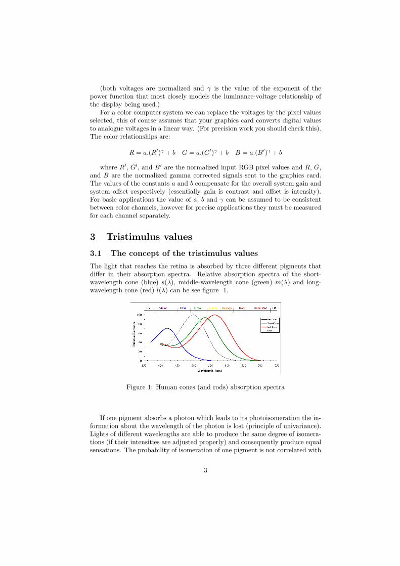
The light that reaches the retina is absorbed by three different pigments thatdiffer in their absorption spectra. Relative absorption spectra of the short-wavelength cone (blue) s(λ), middle-wavelength cone (green) m(λ) and long-wavelength cone (red) l(λ) can be see figure 1.

Figure 1: Human cones (and rods) absorption spectra

If one pigment absorbs a photon which leads to its photoisomeration the in-formation about the wavelength of the photon is lost (principle of univariance).Lights of different wavelengths are able to produce the same degree of isomera-tions (if their intensities are adjusted properly) and consequently produce equalsensations. The probability of isomeration of one pigment is not correlated with

3

the probability of isomeration of another pigment. The probability of isomer-ation is just determined by the wavelengths of the incident photons. If we donot think about the influences of the spatial and temporal effects that influenceperception, the sensation of color is determined by the number of isomerationsin the three types of pigments. Therefore colors can be described by just threenumbers, the tristimulus values, independent of their spectral compositions thatlead to these three numbers.

3.2 The Tristimulus Values

The tristimulus values T for a complex light I(λ) (light that is not monochro-matic) can be calculated for the specific primaries P with their correspondingcolor matching functions Pi(λ):

T1 =∫

λ

P1(λ).I(λ).dλ T2 =∫

λ

P3(λ).I(λ).dλ T3 =∫

λ

P2(λ).I(λ).dλ

3.3 Consequences

1. The amount of excitation of the three pigment types for a complex lightstimulus I(λ) can be calculated:

Sexc =∫

λ

s(λ).I(λ).dλ Mexc =∫

λ

m(λ).I(λ).dλ Lexc =∫

λ

l(λ).I(λ).dλ

2. The amount of excitation of each pigment type to a stimulus P (λ) can becalculated:

Sexc =∫

λ

s(λ).P (λ).dλ Mexc =∫

λ

m(λ).P (λ).dλ Lexc =∫

λ

l(λ).P (λ).dλ

Each primary has a defined overlap in the absorption spectra of the threepigments and consequently leads to a defined sensation. An increase inintensity of one primary reduces to the multiplication with a scalar foreach pigment. Now, because of the principle of univariance, we can addthe influences of the three primaries to the resulting excitations of thethree pigment types.

3. Because of 2, there exists a linear transformation between the tristimulusvalues of a set of primaries and the color space formed by the isomerationsof the cone pigments.

Tristimulus values describe the whole sensation of a color. There exist a lotof other possibilities to describe the sensation of color. For example it is possibleto use something equivalent to cylinder coordinates where a color is expressedby hue, saturation and luminance. If the luminance or the absolute intensity of acolor is not of interest then a color can be expressed in chromaticity coordinates.

4

3.4 Chromaticity Coordinates

In order to calculate the tristimulus values T of a light stimulus due to a set ofprimaries we need to know the spectral shape of the color matching functionsand of the stimulus. The tristimulus values are calculated by the integration ofthe product of the color matching function and the stimulus over the wavelength.The tristimulus values describe the sensation of the stimulus due to the set ofprimaries including the absolute intensities of the three primaries needed tomatch the stimulus. Of course the luminance of that stimulus could be variedwithout changing the hue and saturation of the stimulus. This is reflected in thechromaticity coordinates c that form a two dimensional space thus luminanceis ignored.

c1 =T1

T1 + T2 + T3c2 =

T2

T1 + T2 + T3c3 =

T3

T1 + T2 + T3

It is not necessary to mention the third coordinate because:

c1 + c2 + c3 = 1

3.5 Spectrum locus

We can read the tristimulus values for the spectral colors as the values of thecolor matching functions. For complex light stimuli we would have to integrate.After that we can calculate the chromaticity coordinates out of the tristimulusvalues. In CIE space the tristimulus values are called X, Y and Z, the chromatic-ity coordinates are called x and y. The curve of the chromaticity coordinates ofthe spectral colors is called the spectrum locus (fig. 2).

The straight line connecting the blue part of the spectrum with the red partof the spectrum does not belong to the spectral colors, but it can be mixed outof the spectral colors just as all colors inside the spectrum locus.

4 Color spaces definitions

Color is the perceptual result of light in the visible region of the spectrum, hav-ing wavelengths in the region of 380 nm to 780 nm. The human retina has threetypes of color photoreceptor cells cone, which respond to incident radiation withsomewhat different spectral response curves. Because there are exactly threetypes of color photoreceptor, three numerical components are necessary andtheoretically sufficient to describe a color.

Because we get color information from image files which contain only RGBvalues we have only to know for each color space the RGB to the color spacetransformation formulae.

5

Figure 2: CIE 1931 xyY chromaticy diagram

4.1 Computer Graphic Color Spaces

Traditionally color spaces used in computer graphics have been designed forspecific devices: e.g. RGB for CRT displays and CMY for printers. They aretypically device dependent.

4.1.1 Computer RGB color space

This is the color space produced on a CRT display when pixel values are appliedto a graphic card or by a CCD sensor (or similar). RGB space may be displayedas a cube based on the three axis corresponding to red, green and blue (seefig. 3(a)).

4.1.2 Printer CMY color space

The CMY color model stands for Cyan, Magenta and Yellow which are the com-plements of Red, Green and Blue respectively. This system is used for printing.CMY colors are called ”subtractive primaries”, white is at (0.0, 0.0, 0.0) andblack is at (1.0, 1.0, 1.0). If you start with white and subtract no colors, you getwhite. If you start with white and subtract all colors equally, you get black (seefig. 3(b)).

4.2 CIE XYZ and xyY color spaces

The CIE color standard is based on imaginary primary colors XYZ i.e. whichdon’t exist physically. They are purely theoretical and independent of device-dependent color gamut such as RGB or CMY . These virtual primary colorshave, however, been selected so that all colors which can be perceived by the

6

(a) RGB color space (b) CMY color space

Figure 3: Visualization of RGB and CMY color spaces

human eye lie within this color space.

The XYZ system is based on the response curves of the three color receptorsof the eye’s. Since these differ slightly from one person to another person, CIEhas defined a ”standard observer” whose spectral response corresponds more orless to the average response of the population. This objectifies the colorimetricdetermination of colors.

XYZ (fig. 4(a)) is a 3D linear color space, and it is quite awkward to workin it directly. It is common to project this space to the X + Y + Z = 1 plane.The result is a 2D space known as the CIE chromaticity diagram (see fig. 2).The coordinates in this space are usually called x and y and they are derivedfrom XYZ using the following equations:

x =X

X + Y + Zy =

Y

X + Y + Zz =

Z

X + Y + Z(1)

As the z component bears no additional information, it is often omitted.Note that since xy space is just a projection of the 3D XYZ space, each pointin xy corresponds to many points in the original space. The missing informationis luminance Y. Color is usually described by xyY coordinates, where x and ydetermine the chromaticity and Y the lightness component of color (fig. 4(b)).

4.2.1 RGB to CIE XYZ Conversion

There are different mathematical models to transform RGB device dependentcolor to XYZ tristimulus values. Conversion from RGB to XYZ can take theform of a simple matrix transformation (equ. 2) or a more complex transfor-mation depending of the hardware used (e.g. to acquire or to display colorinformation).

7

In this section we will define how to compute a linear transformation model.This model may by a correct approximation for CCD sensor (RGB to XYZtransform) and CRT display (XYZ to RGB transform). But do not forget, thisis only an approximate model.

RGB

= A.

XYZ

(2)

We can use for example this transformation:

RGB

=

3.06322 −1.39333 −0.475802−0.969243 1.87597 0.04155510.0678713 −0.228834 1.06925

.

XYZ

and the inverse transform simply uses the inverse matrix.

XYZ

=

3.06322 −1.39333 −0.475802−0.969243 1.87597 0.04155510.0678713 −0.228834 1.06925

−1

.

RGB

This is all very useful, but the interesting question is ”Where do these num-bers come from?”. Figuring out the numbers to put in the matrix is the hardpart. The numbers depend on the color system of the output device we areusing. The important parts of a color system are the x and y chromaticitycoordinates and the luminance component of the primaries (xyY ). However, ifwe don’t know the Y values, which is often the case, then we have a problem.However, we can solve this problem if we know the chromaticity coordinates ofthe white point. In the previous example we have used a the color system whichhas the following specifications:

Coordinate xRed yRed xGreen yGreen xBlue yBlue

Value 0.64 0.33 0.29 0.60 0.15 0.06

Coordinate xWhite yWhite YWhite

Value 0.3127 0.3291 1

These terms will be abbreviated to xr, yr, xg, yg, xb, yb, xw, yw and Yw. Weknow already that the relation 1 links the tristimulus values to the chromaticitycoordinates.

We can transform these relations:

X =x

yY Z =

z

yY

The first step is to use these relationships to determine the luminance Yvalues. So we can calculate the tristimulus values as follows

8

Xr = Yr

yrxr Xg = Yg

ygxg Xb = Yb

ybxb

Yr = Yr Yg = Yg Yb = Yb

Zr = Yr

yrzr Zg = Yg

ygzg Zb = Yb

ybzb

For the tristimulus values of the white point:

Xw = xw

ywYw = Yw Zw = zw

yw

We now make the assumption that the sum of full intensity values of redgreen and blue will be white. Using this assumption we can write this relation-ship:

Xw = Xr + Xg + Xb

Yw = Yr + Yg + Yb

Zw = Zr + Zg + Zb

We can then substitute the previous equations to the current one and thenrewrite this latter as a matrix relationship:

xw

ywY w

Y wzw

ywY w

=

xr

yr

xg

yg

xb

yb

1.0 1.0 1.0zr

yr

zg

yg

zb

yb

.

Yr

Yg

Yb

This matrix can be re-written as follows:

Yr

Yg

Yb

=

xr

yr

xg

yg

xb

yb

1.0 1.0 1.0zr

yr

zg

yg

zb

yb

−1

.

xw

ywY w

Y wzw

ywY w

We now have the luminance values Yr, Yg, Yb and we can substitute thesevalues into the previous equations to find Xr, Xg, Xb, Zr, Zg, and Zb. The finalstep is to define the relationship between tristimulus values and RGB valuesas follows. The RGB matrix R should be the result of a multiplication of theconversion matrix C by the tristimulus matrix T :

1 1 0 01 0 1 01 0 0 1

=

? ? ?? ? ?? ? ?

Xw Xr Xg Xb

Yw Yr Yg Yb

Zw Zr Zg Zb

Then the conversion matrix can be calculated as follows

C = R ∗ TT ∗ (T ∗ TT )−1

If we follow this procedure using the values given in the previous examplethen we arrive at the following solution:

C =

3.06322 −1.39333 −0.475802−0.969243 1.87597 0.04155510.0678713 −0.228834 1.06925

9

(a) XYZ color space (b) xyY color space

Figure 4: Visualization of XYZ and xyY color spaces

4.2.2 Chromaticity coordinates of phosphors

Name xr yr xg yg xb yb White pointShort-Persistence 0.61 0.35 0.29 0.59 0.15 0.063 N/ALong-Persistence 0.62 0.33 0.21 0.685 0.15 0.063 N/ANTSC 0.67 0.33 0.21 0.71 0.14 0.08 Illuminant CEBU 0.64 0.33 0.30 0.60 0.15 0.06 Illuminant D65Dell 0.625 0.340 0.275 0.605 0.150 0.065 9300 KSMPTE 0.630 0.340 0.310 0.595 0.155 0.070 Illuminant D65HB LEDs 0.700 0.300 0.170 0.700 0.130 0.075 xw=.31 yw=.32

4.2.3 Standard white points

Name xw yw

Illuminant A 0.44757 0.40745Illuminant B 0.34842 0.35161Illuminant C 0.31006 0.31616Illuminant D65 0.3127 0.3291Direct Sunlight 0.3362 0.3502Light from overcast sky 0.3134 0.3275Illuminant E 1/3 1/3

4.3 A better model for RGB to CIE XYZ conversion

ColorSpace enables user to apply a more accurate model for RGB to CIE XYZconversion. This model (equ. 3) includes an offset suitable to calibrate CCD orCMOS sensors.

10

XYZ

= A.

RGB

+

Xoffset

Yoffset

Zoffset

(3)

4.4 CIE L∗a∗b∗ and CIE L∗u∗v∗ color spaces

There are based directly on CIE XYZ (1931) and are another attempt tolinearize the perceptibility of unit vector color differences. there are non-linear,and the conversions are still reversible. Coloring information is referred to thecolor of the white point of the system. The non-linear relationships for CIEL∗a∗b∗ (see equ. 4 and fig. 5(a)) are not the same as for CIE L∗u∗v∗ (see equ. 7and fig. 5(b)), both are intended to mimic the logarithmic response of the eye.

L∗ = 116(

YY0

) 13 − 16 if Y

Y0> 0.008856

L∗ = 903.3(

YY0

)if Y

Y0≤ 0.008856

a∗ = 500[f( X

X0)− f( Y

Y0)]

b∗ = 200[f( Y

Y0)− f( Z

Z0)]

(4)

with {f(U) = U

13 if U > 0.008856

f(U) = 7.787U + 16/116 if U ≤ 0.008856(5)

and

U(X,Y, Z) =4X

X + 15Y + 3Zet V (X, Y, Z) =

9Y

X + 15Y + 3Z(6)

L∗ = 116(

YY0

) 13 − 16 if Y

Y0> 0.008856

L∗ = 903.3(

YY0

)if Y

Y0≤ 0.008856

u∗ = 13L∗[U(X,Y, Z)− U(X0, Y0, Z0)

]

v∗ = 13L∗[V (X, Y, Z)− V (X0, Y0, Z0

](7)

4.5 Color spaces used in video standards

Y UV and Y IQ are standard color spaces used for analogue television transmis-sion. Y UV is used in European TVs (see fig. 6(a)) and Y IQ in North AmericanTVs (NTSC) (see fig. 6(b)). Y is linked to the component of luminance, andU, V and I, Q are linked to the components of chrominance. Y comes from thestandard CIE XYZ.

11

(a) L∗a∗b∗ color space (b) L∗u∗v∗ color space

Figure 5: Visualization of L∗a∗b∗ and L∗u∗v∗ color spaces

(a) Y UV color space (b) Y IQ color space

Figure 6: Visualization of Y UV and Y IQ color spaces

12

RGB to Y UV transformation

Y = 0.299×R + 0.587×G + 0.114×BU = −0.147×R− 0.289×G + 0.436×BV = 0.615×R− 0.515×G− 0.100×B

RGB to Y IQ transformation

Y = 0.299×R + 0.587×G + 0.114×BI = 0.596×R− 0.274×G− 0.322×BQ = 0.212×R− 0.523×G + 0.311×B

With these formulae the Y range is [0; 1], but U, V, I, and Q can be as wellnegative as positive.

Y CbCr (see fig. 4.5) is a color space similar to Y UV and Y IQ. The trans-formation formulae for this color space depend on the recommendation used.We use the recommendation Rec 601-1 which gives the value 0.2989 for red, thevalue 0.5866 for green and the value 0.1145 for blue.

Figure 7: Y CbCr color space

RGB to Y CbCr transformation

Y = 0.2989×R + 0.5866×G + 0.1145×BCb = −0.1688×R− 0.3312×G + 0.5000×BCr = 0.5000×R− 0.4184×G− 0.0816×B

4.6 Linear transformations of RGB

4.6.1 I1I2I3 color space

Ohta [3] introduced, after a colorimetric analysis of 8 images, this color space.This color space is a linear tranformation of RGB (see fig. 4.6.1).

13

Figure 8: I1I2I3 color space

RGB to I1I2I3 transformation

I1 = 13 (R + G + B)

I2 = 12 (R−B)

I3 = 14 (2G−R−B)

4.6.2 LSLM color space

This color space is a linear transformation of RGB based on the opponent signalsof the cones: black–white, red–green, and yellow–blue (see fig. 4.6.2).

RGB to LSLM transformation

L = 0.209(R− 0.5) + 0.715(G− 0.5) + 0.076(B − 0.5)S = 0.209(R− 0.5) + 0.715(G− 0.5)− 0.924(B − 0.5)

LM = 3.148(R− 0.5)− 2.799(G− 0.5)− 0.349(B − 0.5)

4.7 HSV and HSI color spaces

The representation of the colors in the RGB and CMY color spaces are designedfor specific devices. But for a human observer, they have not accurate defini-tions. For user interfaces a more intuitive color space is preferred. Such colorspaces can be:

• HSI ; Hue, Saturation and Intensity, which can be thought of as a RGBcube tipped up onto one corner (see fig. 10(b) and equ. 8).

14

Figure 9: LSLM color space

(a) HSV color space (b) HSI color space

Figure 10: Visualization of HSV and HSI

15

RGB to HSI transformation

H = arctan(βα )

S =√

α2 + β2

I = (R + G + B)/3(8)

with{

α = R− 12 (G + B)

β =√

32 (G−B)

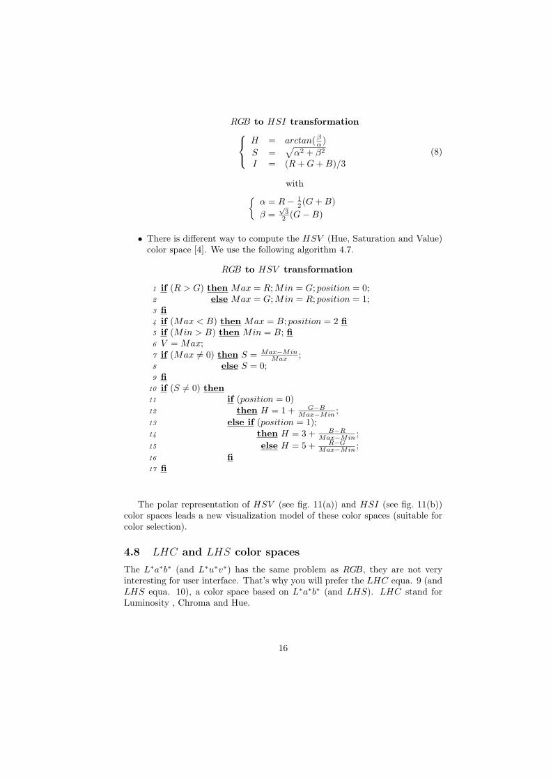
• There is different way to compute the HSV (Hue, Saturation and Value)color space [4]. We use the following algorithm 4.7.

RGB to HSV transformation

1 if (R > G) then Max = R; Min = G; position = 0;2 else Max = G;Min = R; position = 1;3 fi4 if (Max < B) then Max = B; position = 2 fi5 if (Min > B) then Min = B; fi6 V = Max;7 if (Max 6= 0) then S = Max−Min

Max ;8 else S = 0;9 fi

10 if (S 6= 0) then11 if (position = 0)12 then H = 1 + G−B

Max−Min ;13 else if (position = 1);14 then H = 3 + B−R

Max−Min ;15 else H = 5 + R−G

Max−Min ;16 fi17 fi

The polar representation of HSV (see fig. 11(a)) and HSI (see fig. 11(b))color spaces leads a new visualization model of these color spaces (suitable forcolor selection).

4.8 LHC and LHS color spaces

The L∗a∗b∗ (and L∗u∗v∗) has the same problem as RGB, they are not veryinteresting for user interface. That’s why you will prefer the LHC equa. 9 (andLHS equa. 10), a color space based on L∗a∗b∗ (and LHS). LHC stand forLuminosity , Chroma and Hue.

16

(a) HSV color space (polar representa-tion)

(b) HSI color space (polar representa-tion)

Figure 11: Visualization of HSV and HSI color spaces (polar representation)

L∗a∗b∗ to LHC transformation

L = L∗

C =√

a∗2 + b∗2

H = 0 whether a∗ = 0H = (arctan(b∗/a∗) + k.π/2)/(2π)

whether a 6= 0 (add π/2 to H if H < 0)and k = 0 if a∗ >= 0 and b∗ >= 0or k = 1 if a∗ > 0 and b∗ < 0or k = 2 if a∗ < 0 and b∗ < 0or k = 3 if a∗ < 0 and b∗ > 0

(9)

L∗u∗v∗ to LHS transformation

L = L∗

S = 13√

(u∗ − u∗w)2 + (u∗ − u∗w)2H = 0 whether u∗ = 0H = (arctan(v∗/u∗) + k.π/2)/(2π)

whether u 6= 0 (add π/2 to H if H < 0)and k = 0 if u∗ >= 0 and v∗ >= 0or k = 1 if u∗ > 0 and v∗ < 0or k = 2 if u∗ < 0 and v∗ < 0or k = 3 if u∗ < 0 and v∗ > 0

(10)

In order to have a correct visualization (with a good dynamic) of LHS andLHC color spaces we used the following color transformations:

17

L∗a∗b∗ to LHC transformation used in ColorSpace

L = L∗

C =√

a∗2 + b∗2

H = 0 whether a∗ = 0H = 180

π (π + arctan( b∗a∗ )

(11)

L∗u∗v∗ to LHS transformation used in ColorSpace

L = L∗

S = 1.3√

(u∗ − u∗w)2 + (v∗ − v∗w)2H = 0 whether u∗ = 0H = 180

π (π + arctan( v∗u∗ )

(12)

(a) LHC color space (b) LHS color space

Figure 12: Visualization of LHC and LHS color spaces

4.9 Spectral (λSY ) color space

λSY is a color space representation based on brightness, dominant wavelengthand saturation attributes. λSY color coordinates are defined from xyY colorcoordinates.

Let us consider the xy chromaticy diagram given by Figure 13(b). Then, anyreal color X that lies within the region enclosed by the spectrum locus line andupper the lines BW and WR can be considered to be a mixture of illuminantW and spectrum light of its dominant wavelength λd which is determined byextending the line WX until it intersects the spectrum locus [9].

Any color Y that lies on the opposite side of the illuminant point and belowthe lines BW and WR can be described both by a dominant wavelength λd and

18

Red

Green

Blue

White

Spectrum locus

d

x

xc

λ

(a)

Red

Green

Blue

White

Spectrum locus

dλ

x

yys

λ

xsmax

max

a−d

(b)

(c) (d)

Figure 13: λSY color space transformation.

19

by its complementary wavelength λcd which is determined by extending the line

Y W until it intersects the line BR (i.e. the purple line).The saturation S is determined in the xy chromaticity diagram, either by

the relative distance of the sample point and the corresponding spectrum pointfrom the illuminant point, either by the relative distance of the sample pointand the corresponding purple point from the illuminant point.

5 Decorrelated hybrid color spaces

The basic idea of hybrid color spaces is to combine either adaptively, eitherinteractively, different color components from different color spaces to: (a) in-crease the effectiveness of color components to discriminate color data, and (b)reduce rate of correlation between color components [2].

It is established that we can all the more reduce, from K to 3, the numberof color dimensions that: (a) most of color spaces are linked the ones to theothers, either by linear transformations or by non-linear transformations, and(b) all color spaces are defined by a 3 dimensional system.

(a) (b) (c) (d) (e)

(f) (g) (h) (i) (j)

Figure 14: (a) RGB Color image, made of 6 regions (Brown, Orange, Yellow,Pink, Green and Dark Green), projected on different color components. (b),(c), (d) R, G, B projections. Among the three R,G, B color components, atmost 3 regions can be identified with the component G. (e), (f), (g) Y, Cb, Cr

projections. Among the three Y, Cb, Cr color components, at most 3 regions canbe identified with the component Y . (h), (i), (j) H, S, V projections. Amongthe three H, S, V color components, at most 3 regions can be identified withthe component H. In combining G, Y, H color components, all regions can beidentified.

Considering that there is a high redundancy between colors components itis, in a general way, quite difficult to define criteria of analysis to compute au-

20

tomatically the most relevant color components corresponding to a selected setof color components. That is the reason why, in order to build a hybrid colorspace, based on K ′ color components, from K selected color components, suchas K ′ << K (see Figure 14), we propose the following method: (1) select Kcolor components, by using a specific interface which enables the user to weighteach selected color components, and build the corresponding image of dimensionK, (2) compute the covariance matrix (of size K ×K) of K color componentsselected, (3) compute the eigenvectors and the eigen values of this matrix, (4)reduce to K ′ the number of color components in computing the K ′ most signif-icant eigen values of the covariance matrix from a principal component analysis(PCA).

Next, the three first principal components computed (i.e. the decorrelatedhybrid colors components) are used to compute the 3D representation whichbest characterizes the image studied (see Figure 15).

(a) Original Image (b) 3D representation of the hybrid colors

Figure 15: Decorrelated hybrid color space visualization

Figures 16 shows some 3D visualization of decorrelated hybrid color spacesin different configurations in 16(b) 1, 16(c) 1 and 16(d) 2

1Using Components R,G and B of RGB, X and Y of XYZ, L, M and S of LMS, cos ofλSY Polar, without weight

1Using Components L∗ and a∗ of L∗a∗b∗, H and C of LHC, H and S of HSI, withoutweight

2Using Components Y of xyY , L∗ of L∗a∗b∗,L of LHC, I of HSI, without weight

21

(a) Parrot image (b)

(c) (d)

Figure 16: Decorrelated hybrid color spaces examples on parrot image

22

6 Decorrelated hybrid color spaces applied toimage database

6.1 Decorrelated hybrid color spaces: an extension

We have introduced the hybrid construction scheme in the precedent paragraph,based on one initial image. This strategy can be easily applied to a list of im-ages, considering the set of images as one unique image.We will use the following notations, and we will suppose (for simplicity of for-mulæ only) all color spaces are normalized.

• S the set of n images and Sl the l-th image.

• K the set of selected color spaces components and Ki the i-th component.

• Kli(x, y) the corresponding value of pixel (x, y) of component Ki of image

Sl.

• Size (Sl) the size in pixel of the image Sl.

Let introduce the Sum and Cross matrix, defined by:

Sumli =

∑

xy∈Sl

Kli(x, y)

Crosslij =

∑

xy∈Sl

Kli(x, y) ∗Kl

j(x, y)

We note, that for one image Sl, the covariance is then defined by:

Covlij =

Crosslij

Size (Sl)− Suml

i

Size (Sl)× Suml

j

Size (Sl)

Then, to expand the formula to n images:

Covij =

∑1≤l≤n Crossl

ij∑1≤l≤n Size (Sl)

−∑

1≤l≤n Sumli∑

1≤l≤n Size (Sl)×

∑1≤l≤n Suml

j∑1≤l≤n Size (Sl)

At this point, the computation of the hybrid color space follows the previ-ously cited steps:

4. principal component analysis;

5. selection of the 3 most significant axis.

We have developed via ICobra and ColorSpace applications a web interfacesystem3 [14] to manage these hybrid color spaces. The process is divided in twosteps:

3Available at: http://www.icobra.info/hybrid.php

23

• Off-line computation. This part intends to compute the main portion ofcalculus required by the hybrid color space computation.

• Online interface. This part intends, via the interface, to select color spacescomponents and images, to complete the calculus, and, then, to show theselected image in the computed hybrid space.

Before describes rapidly these two parts, we can note: all color spaces are nor-malized during the computation (there is a scale rapport from 1 to 200 betweensome spaces); the transfer values (primaries and white settings) used are, at thismoment, still approximation.

6.2 Off-line computation

Figure 17: Off-line scheme

The figure 17 illustrates the off-line computation. For each image, we willcompute and store:

• for each couple of color spaces components, the Cross value corresponding.It results a m×m matrix, where t is the number of possible color spacescomponents, presently 72 (3× 24) components.

• for each color spaces components, the Sum value corresponding. It resultsa vector of size m.

• the size of image.

6.3 Online interface

As shown in 17 the application may be split into several sections:

• World Wide Web Interface, as figure 19 illustrates. It permits:

– to browse the different image databases;

– to select by clicks a list of images. An empty list means that thedecorrelated hybrid color space is computed on self-image, as usual;

24

Figure 18: Overall online scheme

Figure 19: WWW interface

25

– to select a list of color spaces components;

– to choose the mode of visualization: 2D image, 3D, or 3D histogram;

– to launch ColorSpace with the selected parameters;

• A computational part: the final covariance matrix is computed, usingpre-calculated data;

• A CSI file generation: a csi file (Color Space Interface) is generated, in-cluding all settings and information in order to compute the PCA anddisplaying the selected visualization;

• ColorSpace launching: ColorSpace is launched by the browser (applica-tion/csi mime-type bind) with the csi file as parameter. The softwarecomputes the PCA, and renders the selected visualization.

Figure 20 illustrates this tool within some screenshots using different imagesand color spaces components.

7 References and lectures

[1] P. Colantoni and A. Tremeau, “3d visualization of color data to analyzecolor images,” in The PICS Conference, (Rochester, USA), May 2003.

[2] N. Vandenbrouke, L. Macaire, and J. G. Postaire, “Color pixels classifi-cation in a hybrid color space,” in Proceedings of IEEE, pp. 176–180,1998.

[3] Y. I. Ohta, T. Kanade, and T. Sakai, “Color information for region seg-mentation,” Computer Graphics and Image Processing, vol. 13, pp. 222–241, 1980.

[4] D. F. Rogers, Procedural Elements for Computer Graphics. Mc Graw Hill,1985.

[5] G. A. Agoston, Color Theory and its Application in Art and Design. Op-tical Sciences, Springer-Verlag, 1987.

[6] CIE, “Parametric effects in colour-difference evaluation,” Tech. Rep. 101,Bureau Central de la CIE, 1993.

[7] CIE, “Technical collection 1993,” tech. rep., Bureau Central de la CIE,1993.

[8] CIE, “Industrial colour-difference evaluation,” Tech. Rep. 116, BureauCentral de la CIE, 1995.

[9] D. L. MacAdam, Color Measurement, theme and variation. Optical Sci-ences, Springer-Verlag, second revised ed., 1985.

[10] G. Wyszecki and W. S. Stiles, Color Science: Concepts and Methods,Quantitative Data and Formulae. John Wiley & sons, second ed., 1982.

26

(a) Original image (b) Selected com-ponents and imageslist

(c) Decorrelated hybrid colorspace representation

(d) (e) (f)

(g) (h) (i)

Figure 20: Decorrelated hybrid color spaces: some examples

27

[11] H. R. Kang, Color Technology for Electronic Imaging Devices. SPIEOptical Engineering Press, 1997.

[12] K. N. Plataniotis and A. N. Venetsanopoulos, Color Image Processingand Application. Springer, 2000.

[13] R. Hall, Illumination and Color in Computer Generated Imagery.Springer-Verlag, 1988.

[14] J. D. Rugna, P. Colantoni, and N. Boukala, “Hybrid color spaces appliedto image database,” vol. 5304, pp. 254–264, Electronic Imaging, SPIE,2004.

28