Color appearance of surfaces viewed through fogmdzmura/pubs/HagedornDZmura2000ColorAppearance.p… · Color appearance of surfaces viewed through fog Perception, 2000, volume 29,

1 IntroductionFog that lies between an observer and a surface modifies the light from the surfacethat reaches the eye. To light reflected from a surface is added light scattered byintervening particles. Can observers take these effects of fog into account when theyjudge surface color? Mahadev and Henry (1999) reported that observers can discountthe increased blueness of lights from distant surfaces caused by atmospheric haze. Wereplicate and extend their finding of color constancy for surfaces viewed through fogin the work reported here.

Our approach originates in earlier work on color transparency. The conditions underwhich one perceives a gray, transparent filter that lies atop a set of surfaces were

Color appearance of surfaces viewed through fog

Perception, 2000, volume 29, pages 1169 ^ 1184

John Hagedorn, Michael D'ZmuraôDepartment of Cognitive Sciences, University of California at Irvine, Irvine, CA 92697, USA;e-mail: [email protected] 15 November 1999, in revised form 27 April 2000

Abstract. How do the colors of surfaces seen through fog depend on the chromatic propertiesof the fog? Prior work (eg Chen and D'Zmura, 1998 Perception 27 595 ^ 608) shows that the colors ofsurfaces seen through a transparent filter can be described by a convergence model. The con-vergence model takes into account color shift and change in contrast. Whether the convergencemodel can also be applied to fog was tested experimentally with an asymmetric matching task.In computer graphic simulation, observers adjusted the color of a surface seen through fog inorder to match the color of a surface seen in the absence of fog. The convergence model fitsthe data well. The results suggest that the color constancy revealed in this task with fog isdescribed best by a model that takes into account both shift in color and change in contrast.

DOI:10.1068/p3007

ô Author to whom all correspondence and requests for reprints should be addressed.

Figure 1. Stimulus configuration. This figure and figure 3 can also be seen on the Perceptionwebsite at http://www.perceptionweb.com/perc1000/hagedorn.html and will be archived on theannual CD-ROM accompanying issue 12 of Perception.

http://www.perceptionweb/per1000/hagedorn.html

mailto:[email protected]

examined systematically by Metelli (1974), Beck (1978), Gerbino et al (1990) and others.Metelli devised a model for transparency perception that involves mixing the lumi-nance properties of overlying filter and underlying surfaces. Da Pos (1989) extendedMetelli's model of transparency perception to the three dimensions of color vision bysubstituting tristimulus values for luminances.

This work was corroborated by observations which show that a shift in the colors ofunderlying surfaces or a change in their contrast can lead to transparency perception(D'Zmura et al 1997). Other systematic changes of colour, like rotations or shears in colorspace, do not. Furthermore, one can perceive transparency even in cases of equiluminousshifts in the colors of surfaces lying under a filter. Equiluminous color shifts are notnatural. They can be generated neither by physical filters, which reduce the amount oflight received from a surface, nor by devices like an episcotister (eg Heider 1932; Beck1978), upon which Metelli's original model was based. Transparency perception in casesof equiluminous color shifts shows clearly that the study of transparency perceptionmust be based on perception itself, rather than on particular physical instantiations.

A convergence model was proposed to take into account these observationsconcerning chromatic prerequisites for transparency perception (D'Zmura et al 1997;Chen and D'Zmura 1998). The model holds that an area of the visual field will appeartransparent if and only if the colors of lights from surfaces along the border of the areaconverge towards a point in color space, as the surfaces pass from outside to within.

Do observers take into account the color shift and change in contrast caused by atransparent filter when judging surface color? The results of asymmetric color matchingexperiments show that they do (D'Zmura et al 2000). With the asymmetric matchingtechnique, the color of a surface viewed under a test condition is adjusted so that itmatches the color of a surface viewed under a reference condition (Wyszecki and Stiles1982; Brainard et al 1997). Observers adjusted, in computer graphic simulation, thecolor of a surface seen behind a transparent filter so that it matched the color of asurface seen in plain view. The convergence model fits the color-matching data verywell, suggesting that observers take into account both the color shift and the contrastchange of the filter when judging surface color.

Can observers discount color shifts and changes in contrast caused by fog? Does theconvergence model help to describe the color appearance of surfaces seen through fog?We use the asymmetric matching technique to answer these questions. The colors of testsurfaces seen through fog are compared to the colors of reference surfaces seen in plainview. The comparison reveals the effects of fog on judgments of surface color and letsone quantify how well observers discount fog properties when judging surface color.A preliminary report of this work was made by Hagedorn and D'Zmura (1999).

2 MethodsObservers viewed two texture-mapped rooms that were positioned beside one anotherin computer graphic simulation (see figure 1). The two rooms were identical, with theexception that the room on the left contained fog and the room on the right did not.In each room was placed a Mondrian placard. The observer performed an asymmetricmatching task by matching in colour appearance the central square of the Mondrian inthe fogged room to the central square of the Mondrian in the unfogged reference room.

2.1 DisplayThe stimuli were presented on a Sony Trinitron GDM 20E21 color monitor, whichobservers viewed binocularly at a distance of 57 cm in a dark room. Software on anSGI O2 computer provided 24 bits of chromatic information for each of the 128061024pixels presented at a field rate of 72 Hz (noninterlaced). The software corrected thenonlinear relationship between applied voltage and phosphor intensity for each gun.

1170 J Hagedorn, M D'Zmura

The chromaticities and luminances of the three phosphors of the monitor were measuredwith a Photo Research PR-650 SpectraColorimeter and are presented in table 1.

2.2 Spatial configurationThe stimulus was presented in a window that subtended 35.5 deg627.1 deg. EachMondrian placard consisted of a five by five array of colored areas, each of uniformcolor and of approximately square shape (see figure 1). The width and height of eachpseudosquare were generated randomly from a distribution uniform on the interval[1.2, 1.8] deg. The square shapes were perturbed in this way in order to avoid unwantedinstances of transparency that arise when squares in uniform arrays are colored randomly(D'Zmura et al 2000).

2.3 Color spaceStimulus color properties are described in the DKL color space (Derrington et al 1984),which is based on the MacLeod and Boynton (1979) color diagram (see figure 2). Theneutral gray point G of this color space was set to the light created by displayingsimultaneously each of the monitor's three phosphors at half intensity. The chromatic-ity of G was (0.27, 0.29), and its luminance was 31.1 cd mÿ2.

The color space has three axes which intersect at the gray point G. The first ofthese axes is the achromatic (A) axis, lights along which are created by generatingequal modulations of the three phosphors about G. The other two axes lie in theequiliminous plane through G; lights in this plane are of equal luminance as definedby the Vl photopic luminosity function (Wyszecki and Stiles 1982). Modulation alongthe LM axis changes the excitations of the L and M cones and is invisible to S cones.Lights along this axis typically have a red or blue ^ green appearance. Modulationalong the S axis changes the excitation of S cones and is invisible both to L and toM cones. Lights along the S axis typically have a purple or yellow ^ green appearance.Below, we specify the length of a vector that lies along a particular half axis in theDKL space in terms of cone contrast (Smith and Pokorny 1975).

Table 1. CIE 1931 standard observer chromaticity (x, y) and maximal luminance Lmax of eachphosphor R, G, and B.

R G B

x 0.621 0.286 0.150y 0.341 0.605 0.062Lmax =cd mÿ2 14.6 52.6 8.28

A

G

y

908S

LM0

f

Figure 2. DKL color space; see text for details

Color appearance of surfaces viewed through fog 1171

2.4 Chromatic propertiesThe pseudosquares for both the test and reference placards had R, G, and B values thatwere drawn randomly from a distribution uniform on the interval [0.25, 0.75] (with 1.0representing maximum possible intensity). For each pseudosquare, other than the centralreference pseudosquare, an independent random draw was performed for each of thethree phosphors on each trial to determine the chromatic properties of the pseudosquare.

The fog was simulated with the convergence model, the intuition for which is asfollows. Suppose that the chromatic properties of the light from a surface seen in plainview are represented by a three-dimensional vector of tristimulus values a. In the presenceof fog, only some of the original light from the surface reaches the eye. The effects of fogcan be simulated by adding some amount of a second light f that depends on thechromatic properties of the fog. The resulting light b that reaches the eye is a combina-tion of the two original lights:

b � �1ÿ a�a� af , (1a)

Figure 3. Various fog conditions. Four uppermost panels: full intensity fog with placard in thefar position. Fog colors shown are, at upper left, `red', along the positive LM half-axis;at upper right, `blue ^ green', along the negative LM half-axis; at middle left, `purple', alongthe positive S half-axis, and at middle right, `yellow ^ green', along the negative S half-axis.The two lowermost panels show, at left, full-intensity gray fog with the placard in the nearposition; and at right, half-intensity fog with the placard in the far position.


in which the contrast reduction parameter a varies from 0 to 1 and represents theamount of fog present: no fog whatsoever (a � 0) through fully opaque fog (a � 1).Physical variations that can cause a to vary include fog density and viewing distancethrough the fog. In an equivalent formulation, one sets the translation t equal to theproduct af and the contrast parameter b equal to 1ÿ a:

b � ba� t . (1b)

The appendix presents a derivation of the convergence model from the radiative-transfer equation for light in a homogeneous scattering medium. This equation describesthe chromatic and the spatial dependence of light from a surface viewed through fog(Middleton 1950; Mahadev and Henry 1999). The radiative-transfer equation can bereduced to the form of equation (1), if one assumes that the fog extinction coefficient isa constant function of wavelength. This assumption is true of natural clouds and fogthat are formed from water vapor (McClatchey et al 1978). The result is a spatiochro-matic convergence model [equations (A6) and (A8)], formulated in terms of tristimulusvalues that takes into account the distance from the observer of the viewed surfacethrough the fog.

OpenGL graphics software was used in these experiments to display the experimentalscene and to simulate the effects of fog. The OpenGL model for fog corresponds to theconvergence model, formulated in terms of R, G, and B values, rather than in termsof tristimulus values (OpenGL ARB et al 1997). OpenGL graphics software allows forfog intensity to depend on fog distribution in depth in either a linear or an exponentialfashion.We used fog with a linear dependence on optical depth in these experiments.Wehave no reason to believe that the results depend in any significant fashion on this choice.

2.5 ConditionsFog color, fog intensity, and test placard position in depth were varied in computergraphic simulation. Twenty conditions were provided by varying factorially five fogcolors, two levels of fog intensity, and two levels of placard position.

2.5.1 Fog color. Five fog colors were chosen, including gray and one for each of the fourcardinal half-axes: �LM (red), ÿLM (blue ^ green), �S (purple), and ÿS (yellow ^ green).These have azimuthal angles 08, 1808, 908, and 2708, respectively, in the equiluminousplane of the DKL color space (figure 2). These colored fogs are shown at full intensity inthe top four panels of figure 3. The RGB equivalents used in the OpenGL softwarefor each color were gray (0.3, 0.3, 0.3), red (0.3282, 0.2360, 0.2590), blue ^ green (0.1531,0.2850, 0.2573), purple (0.2645, 0.2393, 0.3510), and yellow ^ green (0.2169, 0.2816, 0.1653).

2.5.2 Placard position. Test placards were presented at `far' and at `near' levels. In afar condition, the placard was placed just in front of the back wall of the room (asshown in figure 1). A support post and a shadow on the back wall were displayed tohelp the observer perceive a distant placement for the placard. In the near condition,the placard was placed at a simulated distance of one-half the length of the room.As shown in the bottom two panels of figure 3, a support post was added to theplacard in near position; no shadow was used. The physical size of the simulatedtest placard was decreased in the near conditions to keep its position on the screenand its projected size in degrees of visual angle identical to that of the placards in thefar conditions. The placard in the fogless reference condition was placed in the farposition.

2.5.3 Fog intensity. Fog was presented at `full' and at `half' intensity levels. These inten-sity levels correspond to choices for the contrast reduction parameter a in equations(1a) and (1b). The value of a in the half-fog conditions was 0.5, when measured foritems placed in the far position, and was 0.25, when measured for items placed in


the near position. The value of a in the full-intensity fog conditions was 0.714, whenmeasured for items in the far position, and was 0.357, when measured for items placedin the near position. One can find the corresponding values for contrast parameter b[equation (1b)] by subtracting each of the values for a from one, giving 0.5, 0.75,0.286, and 0.643, respectively.

2.6 ObserversThree color-normal observers, two of whom (JH and MD) are authors, matchedseventeen reference colors, arrayed in the equiluminous plane about the neutral graypoint, for each of the twenty conditions. Reference color chromaticity coordinates areprovided in table 2 and are plotted in figure 4 as filled circles. The task was to match

Table 2. CIE 1931 standard observer chromaticities of the seventeen reference stimuli. Eachreference stimulus was of luminance 31.1 cd mÿ2.

1 2 3 4 5 6 7 8 9

x 0.2994 0.2739 0.2515 0.238 0.2406 0.267 0.3044 0.3163 0.2856y 0.2772 0.2384 0.2296 0.2502 0.3005 0.3649 0.3877 0.3403 0.2827

10 11 12 13 14 15 16 17

x 0.2727 0.2602 0.2534 0.2562 0.2693 0.2853 0.2919 0.2712y 0.2610 0.2556 0.2679 0.2943 0.3221 0.3307 0.3122 0.2884

JH S GL S

MD S CC S

LM LM

LM LM

Figure 4. Results of color-matching for red fog. For each of the seventeen reference colors, shownby the filled circles, observers JH, GL, and MD made six settings whose averages are shown bythe unfilled circles. The bottom right panel labeled CC shows the settings expected of a fullycolor-constant observer. The gray diamond in the bottom right panel along the LM axis showsthe red target of convergence. Reference color chromaticities are given in table 2.


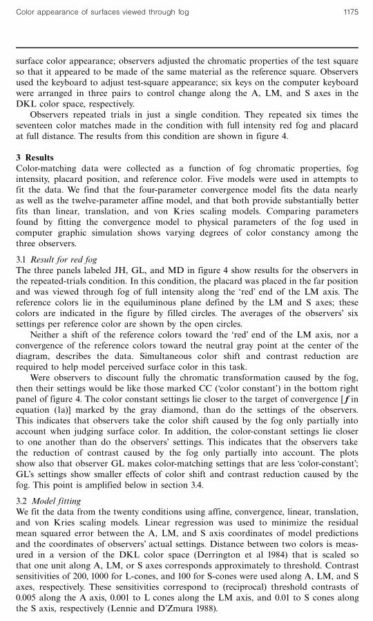
surface color appearance; observers adjusted the chromatic properties of the test squareso that it appeared to be made of the same material as the reference square. Observersused the keyboard to adjust test-square appearance; six keys on the computer keyboardwere arranged in three pairs to control change along the A, LM, and S axes in theDKL color space, respectively.

Observers repeated trials in just a single condition. They repeated six times theseventeen color matches made in the condition with full intensity red fog and placardat full distance. The results from this condition are shown in figure 4.

3 ResultsColor-matching data were collected as a function of fog chromatic properties, fogintensity, placard position, and reference color. Five models were used in attempts tofit the data. We find that the four-parameter convergence model fits the data nearlyas well as the twelve-parameter affine model, and that both provide substantially betterfits than linear, translation, and von Kries scaling models. Comparing parametersfound by fitting the convergence model to physical parameters of the fog used incomputer graphic simulation shows varying degrees of color constancy among thethree observers.

3.1 Result for red fogThe three panels labeled JH, GL, and MD in figure 4 show results for the observers inthe repeated-trials condition. In this condition, the placard was placed in the far positionand was viewed through fog of full intensity along the `red' end of the LM axis. Thereference colors lie in the equiluminous plane defined by the LM and S axes; thesecolors are indicated in the figure by filled circles. The averages of the observers' sixsettings per reference color are shown by the open circles.

Neither a shift of the reference colors toward the `red' end of the LM axis, nor aconvergence of the reference colors toward the neutral gray point at the center of thediagram, describes the data. Simultaneous color shift and contrast reduction arerequired to help model perceived surface color in this task.

Were observers to discount fully the chromatic transformation caused by the fog,then their settings would be like those marked CC ( c̀olor constant') in the bottom rightpanel of figure 4. The color constant settings lie closer to the target of convergence [ f inequation (1a)] marked by the gray diamond, than do the settings of the observers.This indicates that observers take the color shift caused by the fog only partially intoaccount when judging surface color. In addition, the color-constant settings lie closerto one another than do the observers' settings. This indicates that the observers takethe reduction of contrast caused by the fog only partially into account. The plotsshow also that observer GL makes color-matching settings that are less c̀olor-constant';GL's settings show smaller effects of color shift and contrast reduction caused by thefog. This point is amplified below in section 3.4.

3.2 Model fittingWe fit the data from the twenty conditions using affine, convergence, linear, translation,and von Kries scaling models. Linear regression was used to minimize the residualmean squared error between the A, LM, and S axis coordinates of model predictionsand the coordinates of observers' actual settings. Distance between two colors is meas-ured in a version of the DKL color space (Derrington et al 1984) that is scaled sothat one unit along A, LM, or S axes corresponds approximately to threshold. Contrastsensitivities of 200, 1000 for L-cones, and 100 for S-cones were used along A, LM, and Saxes, respectively. These sensitivities correspond to (reciprocal) threshold contrasts of0.005 along the A axis, 0.001 to L cones along the LM axis, and 0.01 to S cones alongthe S axis, respectively (Lennie and D'Zmura 1988).


Five models were fit to the data: affine, convergence, linear, translation, and von Kriesscaling. The affine model is described by the equation

b �Ma� t , (2)

in which a is a three-dimensional vector of reference color coordinates, M is a 363matrixdescribing a linear transformation, t is a three-dimensional translation vector, and b isa predicted vector of test color coordinates (Jameson and Hurvich 1964; Brainard et al1997). When fitting the model to the color-matching data found by an observer in aparticular condition, one chooses the entries of the matrix M and the vector t so asto minimize the RMS error between the predictions and an observer's actual settings.The affine model has twelve parameters that may be adjusted during the fitting proce-dure: nine for the 363 linear transformation M and three for the color shift t.

The convergence model [equation (1b)] is a special case of the affine model withonly four parameters. The linear model, too, is a special case of the affine model andis formulated by removing the translation t from equation (2):

b �Ma . (3)

Likewise, the translation model is a special case found by removing the linear trans-formation M from equation (2):

b � a� t . (4)

The von Kries (1905) scaling model, finally, can be expressed by the equation

b 0 � Da 0 , (5)

in which a 0 is a vector of reference color L-, M-, and S-cone excitations, and D is adiagonal matrix that scales the cone excitations to produce the cone excitations b 0

predicted by the model. To fit data with this model, color specifications in the DKLspace are first converted into the LMS space of cone excitations. One then attemptsto fit the data using three factors to scale the respective cone excitations. The resultsare then converted from the LMS space back to the DKL space so that they may becompared with the fits of the other models.

3.3 Model fitsFigure 5 shows the sum of residual mean squared errors for the three observers JH,MD, and GL. The models are indicated below the horizontal axis by their first letter:Aöaffine, Cöconvergence, Lölinear, Tötranslation, and Sövon Kries scaling. Betterfits correspond to smaller residual error values.

The affine model (leftmost columns) fits the data best; indeed, the affine modelmust perform at least as well as the other models, because the others are all instances

35

30

25

20

15

10

5

0

Residua

lerror

A C L T SModel

JH

MD

GL

Figure 5. Model fits for the color conditions,by observer. Each column lists the sum ofresidual mean squared errors found in fittinga model to each of the twenty conditions.The model is listed by its first letter along thehorizontal axis: affine (A), convergence (C),linear (L), translation (T), scaling (S).


of it. The results show also that the convergence model fits the data nearly as well asthe affine model, and that the other three models fit the data less well. The similarityin the abilities of the affine and convergence models to fit the data suggests that theeight extra degrees of freedom within the linear transformation of the affine model donot account for much variance in the data beyond that accounted for by the contrast-reduction parameter. Note also that the fits to GL's data by the linear, translation,and scaling models are better than the fits to the data of JH and MD by these models.

Figure 6 shows that there is no significant dependence of the quality of fits onfog color.

The effect of fog intensity on the model fits are shown in figure 7. Again, the affine andconvergence models fit the data substantially better than the linear, translation, and scalingmodels. The affine and convergence model fits are slightly better in the full-intensity fogconditions than in the half-intensity fog conditions. The other modelsölinear, translation,and scalingöfail to fit the data, especially in the full-intensity conditions.

Figure 8 shows the effects of placard position on the model fits. The affine andconvergence models fit the data well, and perform slightly better for the far-placardconditions than for the near-placard positions. The linear, translation, and von Kriesmodels fit the data less well, but perform better for the near-placard condition.

gray

yellow ^ green

purple

blue ^ green

red

20

15

10

5

0

Residua

lerror

A C L T SModel

Figure 6. Fog color has little effect on model fits. Each column lists the sum of residual meansquared errors found in each of four conditions per color, averaged across the three observers.Model labels are as in figure 5.

70

60

50

40

30

20

10

0

Residua

lerror

A C L T SModel

full

half

Figure 7. Effects of fog intensity onmodel fits. Each column lists the sumof residual mean squared errors foundin each of ten conditions per intensity,averaged across the three observers.Model labels are as in figure 5.


The results for fog intensity and for placard position shown in figures 7 and 8,respectively, indicate that the affine and convergence models fit the color-matchingdata better in conditions with relatively more intervening fog, as in the full-intensityand far-placard conditions. Conversely, the linear, translation, and von Kries modelsperform better in conditions with relatively less intervening fog. The affine and con-vergence models fit best in all conditions.

3.4 Color constancy resultsOne can use the fits to data provided by the convergence model to estimate the degreeof color constancy exhibited by each observer at each condition. The fits provideestimates of the scalar contrast parameter b̂ and the vector color shift parameter t̂[equation (2)] required for the fit by the convergence model.

Figure 9 shows scatter plots, for each observer, of the estimates b̂ of perceived contrastversus the actual values b required to generate the fogs in the various experimentalconditions. Each point in the plot represents a pair of perceived and actual contrastvalues, found for each observer and for each condition. The Pearson product momentcorrelation coefficients for each observer are given in table 3. Perceived and actualcontrast are highly correlated; the correlation coefficients range from 0.94 to 0.96.

The best-fit lines have slopes 0.80 (GL), 1.01 (MD), and 1.14 (JH), while the interceptsare 0.34 (GL), ÿ0.06 (MD), and ÿ0:06 (JH). The intercepts are of negligible value, with theexception of that for observer GL. The two observers JH and MD evidently take thecontrast properties of fog into account fully when judging surface color. There is a

70

60

50

40

30

20

10

0

Residua

lerror

A C L T SModel

near

far

Figure 8. Effects of placard posi-tion on model fits. Each columnshows the sum of residual meansquared errors found in each often conditions per simulated dis-tance, averaged across the threeobservers. Model labels are as infigure 5.

1.0

0.8

0.6

0.4

0.2

0

Perceivedcontrast

GL

JH

MD

0 0.2 0.4 0.6 0.8 1.0Actual contrast

Figure 9. Plot of perceived contrastversus actual contrast for observersGL (diamonds), JH (triangles),and MD (squares). Estimates b̂ ofthe contrast parameters for eachobserver for each condition, foundby fitting the convergence modelto observers' data, are plottedagainst the actual, physical con-trasts b of the fogs simulated incorresponding conditions. Param-eters of the best-fit lines are givenin table 3.


nearly one-to-one correspondence between the contrast estimates b̂ and the actual val-ues b for observers JH and MD. While the slope for observer GL is also high, this isoffset by the high value of the intercept, so that the estimates of perceived contrast b̂are uniformly higher than the actual values. Higher values indicate that reduction ofcontrast by fog is not taken fully into account by GL. Recall that the parameter b ofthe convergence model [equation (1b)] reports surface contrast: a value of 1 for bcorresponds to no reduction in the contrast of the surface, while a value of 0 corre-sponds to a total reduction in contrast. The higher estimates b̂ for GL thus correspondto smaller estimates of perceived contrast reduction.

In figure 10 are shown scatter plots of estimated and actual lengths of color shiftvectors. Each point represents an estimate of the length of the perceived color shift foundby fitting the convergence model to an observer's data in an experimental condition(vertical axis) and the actual length (horizontal axis). Table 4 shows the correlation

Table 3. Correlation between the estimates b̂ found by fitting the convergence model to the dataof observers JH, MD, and GL and the actual contrast reduction b of the fogs used in the twentyexperimental conditions. Shown are Pearson product moment correlations, as well as the slopesand intercepts of best-fitting lines (pictured in figure 9).

JH MD GL

Correlation 0.942 0.955 0.963Slope 1.138 1.013 0.800Intercept ÿ0.061 ÿ0.064 0.337

40

30

20

10

0

Perceivedleng

th

0 10 20 30 40Actual length

JH

MD

GL

Figure 10. Plot of magnitude of perceivedcolor shift versus magnitude of actual colorshift for observers GL (diamonds), JH (tri-angles), and MD (squares). Estimates ofthe lengths of the perceived color shifts t̂ foreach observer for each condition, found byfitting the convergence model to observers'data, are plotted against the lengths of theactual color shifts t of the fogs simulatedin corresponding conditions. Parameters ofthe best-fit lines are given in table 4.

Table 4. Correlation between the lengths of perceived color shifts t̂ fit to the data of observersJH, MD, and GL, and the lengths of actual color shifts t. Shown are Pearson product momentcorrelations, as well as the slopes and intercepts of best-fitting lines (pictured in figure 10). Theintercepts are shown in threshold-scaled units.

JH MD GL

Correlation 0.778 0.555 0.607Slope 0.780 0.623 0.292Intercept ÿ0.133 3.171 2.002


coefficients for each observer. They range from 0.56 to 0.78 and, although less high invalue than those for contrast reduction, they are significant. The slopes and intercepts ofthe best-fit lines are given in table 4 also. The intercepts, which are reported in threshold-scaled units, are negligible in value. The slopes for MD and JH are 0.62 and 0.78,respectively, while that for GL is 0.29. These slopes suggest that the first two observerstake between 60%^ 80% of the actual color shift into account when judging surface color.The third observer, GL, takes about 30% of the shift into account, so evincing less colorconstancy, which agrees with the perceived contrast results found for this observer.

The azimuthal angles of perceived color shifts within the equiluminous plane arecompared to the azimuthal angles of the actual color shifts in figure 11. Actual azimuthalangles of the fog stimuli were 08 for �LM (`red'), 908 for �S (`purple'), 1808 for ÿLM(`blue ^ green'), and 2708 for ÿS (`yellow ^ green'). The correlations for the three observersare uniformly very high (see table 5). The plot shows that observers made settings that,for the most part, agreed very closely with the actual azimuths. The points in the plotlie close to the diagonal line, which has a slope of 1 and an intercept of 0.

4 DiscussionThe results of these asymmetric color-matching experiments show that observers takeinto account the chromatic properties of fog when judging surface color. Observersdiscount two aspects of the chromatic properties of fog: reduction in contrast and shiftin the colors of lights from surfaces. Two of the observers in this study discountedcontrast reduction fully, and discounted somewhere between 60% ^ 80% of the color

360

270

180

90

0

ÿ90

Perceivedazim

uth=

8

90 180 270 360Actual azimuth=8

Figure 11. Plot of azimuthal angleof perceived color shift versus azi-muthal angle of actual color shiftfor observers GL (diamonds), JH(triangles), and MD (squares).Estimates of the azimuthal angles,within the equiluminous plane, ofthe perceived color shifts t̂ foreach observer for each conditionare plotted against the azimuthalangles of the actual color shifts t.Actual azimuthal angles were 08(�LM, `red'), 908 (�S, `purple'),1808 (ÿLM, `blue ^ green') and 2708(ÿS, `yellow-green'). The diagonal linehas slope 1 and intercept 0.

Table 5. Correlation between the azimuthal angles in the equiluminant plane of color shifts t̂ fitto the data of observers JH, MD, and GL, and the azimuthal angles of fog actual color shifts t.

JH MD GL

Correlation 0.991 0.975 0.937


shift. These two observersöthe authorsöexhibit nearly complete color constancy. Theother, na|« ve, observer, discounted contrast reduction and color shift only partially.

In all cases, the convergence model fit the data nearly as well as the affine model,even though the affine model has twelve parameters and the convergence model hasonly four. Linear, translation, and von Kries scaling models fit the data considerablyless well in all cases. That the asymmetric color-matching data are fit well by theconvergence model suggests that observers take into account both contrast reductionand shift in color when judging the colors of surfaces seen through fog.

It may seem tautological to test a convergence model of visual processing with fogstimuli that are modeled in the same way. Yet it need not have been the case that thevisual system takes fog contrast reduction and color shift into account when judgingsurface color. For instance, were our visual systems unable to take into account fogcontrast reduction, then translation and von Kries scaling models would have donejust as well in fitting the data as the more general convergence and affine models. Yetthe results of the present experiments show convincingly that observers do take contrastvariation into account when judging surface color.

A similar result was found in recent experiments on the colors of surfaces seento lie behind a transparent filter (D'Zmura et al 2000). Observers took into accountboth contrast reduction and color shift caused by such a filter. Asymmetric color matchesshowed that approximately one-half of the reduction of contrast and one-half of the colorshift caused by a transparent filter were taken into account by the observers. Again, theconvergence model fit the data nearly as well as the affine model and performedsubstantially better than linear, translation, or von Kries scaling models.

Fog differs from a transparent filter in two ways. First, the chromatic effects offog increase with depth, as the amount of fog intervening between surface and viewerincreases. Unlike a transparent filter, fog imposes a chromatic transformation on under-lying surfaces that depends strongly on the depth of a surface behind the filter. Second,fog tends to have poorly defined borders, while transparent filters tend to have clearly-demarcated borders defined by sharp edges and X-junctions (Heider 1932).

Common to both fog and a transparent filter are the scission or perceived layeringin depth of the visual field into chromatic processes (Faul 1997; Mausfeld 1998). Thelayers include opaque surfaces, seen to lie farther away from the observer, and interveningchromatic processes like illumination, transparency, and fog. Our results with trans-parency and with fog suggest that the convergence model describes the color appearanceof surfaces in cases of scission (D'Zmura et al, in press). Observers can discount both shiftin color and change in contrast caused by an intervening color process.

Observers match color in these experiments by finding the color for the test surface,seen through an intervening color process, that causes it to appear to be made of the samestuff as the reference surface. Such a `paper' or surface-color match differs from ac̀olorimetric' match, for which one attempts to set the color of the test area so that itmatches the color of the reference area, independently of context provided by surroundingelements (Arend and Reeves 1986). The two situations that are compared by observers inexperiments with fog and with transparency involve highly visible color differences.

That we are able to take into account changes in contrast when judging surfacecolor was first pointed out by Brown and MacLeod (1992). There are two potentialways in which such a compensation may be done. The first is an automatic contrastgain control, which is known to operate within both achromatic and color-opponentchannels [see review by D'Zmura and Singer (1999)]. This automatic compensation hasbeen studied by colorimetric matches. The second is through a conscious judgmentconcerning visible processes; this has been studied here with surface-color matches.


Acknowledgements. We thank an anonymous referee for help in clarifying the relationshipbetween the Beer ^ Lambert law and the radiative transfer equation. This work was supported byNIH EY10014 and by NSF DB9724595.

ReferencesArend L E, Reeves A, 1986 `̀ Simultaneous color constancy'' Journal of the Optical Society of

America A 3 1743 ^ 1751Beck J, 1978 `̀Additive and subtractive color mixture in color transparency'' Perception & Psycho-

physics 23 265 ^ 267Brainard D H, Brunt W A, Speigle J M, 1997 `̀ Color constancy in the nearly natural image.

1. Asymmetric matches'' Journal of the Optical Society of America A 14 2091 ^ 2110Brown R O, MacLeod D I A, 1992 `̀ Saturation and color constancy'', in Advances in Color Vision

Technical Digest (Washington, DC: Optical Society of America) pp 110 ^ 111Chen V J, D'Zmura M, 1998 `̀ Test of a convergence model for color transparency perception''

Perception 27 595 ^ 608Da Pos O, 1989 Transparenze (Padua: Icone)Derrington A M, Krauskopf J, Lennie P, 1984 `̀ Chromatic mechanisms in lateral geniculate nucleus

of macaque'' Journal of Physiology (London) 357 241 ^ 265D'Zmura M, Colantoni P, Hagedorn H, in press `̀ Perception of color change'' Color Research

and ApplicationD'Zmura M, Colantoni P, Knoblauch K, Laget B, 1997 `̀ Color transparency'' Perception 26

471 ^ 492D'Zmura M, Rinner O, Gegenfurtner K R, 2000 `̀ The colors seen behind transparent filters''

Perception 29 911 ^ 926D'Zmura M, Singer B, 1999 `̀ Contrast gain control'', in Colour Vision: From Genes to Perception

Eds L T Sharpe, K R Gegenfurtner (Cambridge: Cambridge University Press) pp 369 ^ 385Faul F, 1997 `̀ Theoretische und experimentelle Untersuchung chromatischer Determinanten per-

zeptueller Transparenz'', Dissertation, Christian-Albrechts-Universita« t zu Kiel, Kiel, GermanyGerbino W, Stultiens C I F H J, Troost J M, Weert C M M de, 1990 `̀ Transparent layer

constancy'' Journal of Experimental Psychology: Human Perception and Performance 163 ^ 20

Hagedorn J B, D'Zmura M, 1999 `̀ Color appearance of surfaces viewed through fog'' InvestigativeOphthalmology & Visual Science 40(4) S750

Heider G M, 1932 `̀ New studies in transparency, form and color'' Psychologische Forschung 1413 ^ 55

Jameson D, Hurvich L M, 1964 `̀ Theory of brightness and color contrast in human vision''Vision Research 4 135 ^ 154

Kries J von, 1905 `̀ Die Gesichtsempfindungen'', in Handbuch der Physiologie des Menschen vol-ume 3 Ed. W Nagel (Braunschweig: Vieweg) pp 109 ^ 279

Lennie P, D'Zmura M, 1988 `̀ Mechanisms of color vision'' Critical Reviews in Neurobiology 3333 ^ 400

McClatchey R A, Fenn R W, Selby J E A, Volz F E, Garing J S, 1978 `̀ Optical properties ofthe atmosphere'', in Handbook of Optics Ed. W G Driscoll (New York: McGraw-Hill)pp 14.1 ^ 14.65

MacLeod D I A, Boynton R M, 1979 ``Chromaticity diagram showing cone excitation by stimuliof equal luminance'' Journal of the Optical Society of America 69 1183 ^ 1186

Mahadev S, Henry R C, 1999 `̀Application of a color-appearance model to vision through atmo-spheric haze'' Color Research and Application 24 112 ^ 120

Mausfeld R, 1998 `̀ Color perception: From Grassmann codes to a dual code for object andilluminant colors'', in Color Vision Eds W Backhaus, R Kliegl, J Werner (Berlin: deGruyter)pp 219 ^ 250

Metelli F, 1974 `̀ The perception of transparency'' Scientific American 230(4) 91 ^ 98Middleton W E K, 1950 `̀ The colors of distant objects'' Journal of the Optical Society of America

40 373 ^ 376OpenGL ARB, Woo M, Neider J, Davis T, 1997 OpenGL Programming Guide second edition

(New York: Addison-Wesley)Smith V C, Pokorny J, 1975 `̀ Spectral sensitivity of the foveal cone photopigments between 400

and 500 nm'' Vision Research 15 161 ^ 171Wyszecki G, Stiles W S, 1982 Color Science. Concepts and Methods, Quantitative Data and Formulae

(New York: John Wiley)


Appendix. A spatiochromatic convergence modelThe radiative transfer equation for light through a homogeneous medium can be usedto describe the spatial and chromatic dependence of light from a surface viewed throughfog. The radiative transfer equation can be reduced to the form of the convergencemodel, if one assumes that the fog extinction coefficient is a constant function of wave-length. This assumption holds true of natural clouds and fog, formed from water vapor(McClatchey et al 1978). The result is a formulation of the convergence model, in termsof cone tristimulus values, that takes into account the distance from the observer ofthe viewed surface through the fog.

The radiative transfer equation for light, assuming a horizontal sight path in ahomogeneous scattering medium, is given by the following equation (Middleton 1950;Mahadev and Henry 1999):

L�x; l� � S�l� exp �ÿt�x; l�� h�l�e�l��

f1ÿ exp �ÿt�x; l��g . (A1)

In this equation, L(x, l) is the radiance of the light reaching the eye and S(l) is theradiance of the light from the surface prior to its passage through the fog. Thevariable x refers to the distance of the viewed surface through uniform fog, and lrefers to visible wavelength. The function of wavelength e(l) in equation (A1) is theextinction coefficient of the fog, and t(x, l) is the optical depth of the viewed surfaceand is related to the extinction coefficient by

t�x; l� � e�l�x . (A2)

The function h(l), finally, describes the light from the air along the line of sight andquantifies scattered light per unit length and volume of fog.

The first term on the right-hand side of equation (A1) describes the light transmittedfrom the surface to the viewer through the fog. It represents the integral form of theBeer ^ Lambert law, on the assumption of a homogeneous medium. The second termdescribes the path radiance, or light that reaches the viewer from the fog that did notoriginate from the surface.

If one assumes that the extinction coefficient e(l) is a constant function e of wave-length, then the optical depth may be expressed simply as a function of distance:

t�x; l� � t�x� � ex . (A3)

The three tristimulus values q1 , q2 , q3 of the light with radiance L(x, l) can bedetermined by integrating the product of the radiance and each of the three spectralsensitivity functions Qi (l), 1 4 i 4 3:

qi �x� � hQi �l�; L(x; l�i; 1 4 i 4 3 , (A4)

in which h j; ki is used as a shorthand for the integral over the visible spectrum ofthe product of two functions of wavelength j and k. Substituting the right-hand side ofequation (A1) for the radiance in equation (A4) and assuming that equation (A3)holds true, one finds that

qi �x� � hQi �l�; S�l�i exp�ÿex� ��Qi �l�;

h�l�e

��1ÿ exp�ÿex�� , (A5)

orqi �x� � exp�ÿex�ai � �1ÿ exp�ÿex�� fi , for 1 4 i 4 3 , (A6)

where

ai � hQi �l�; S�l�i (A7a)


and

fi ��Qi �l�;

h�l�e

�, 1 4 i 4 3 . (A7b)

Equation (A6) has the form of the convergence model but specifies the spatial depen-dence of the tristimulus values.

The integrals in equation (A5) would not separate nicely were the extinctioncoefficient to depend on wavelength. In that case, the optical depth t would depend onwavelength and would remain inside the integral with the spectral sensitivity function(Middleton 1950). The assumption of a constant extinction coefficient allows one toseparate spatial from spectral forms in the radiative transfer equation to provide aspatiochromatic convergence model [equation (A6)].

A simple generalization lets one model a non-exponential fall-off of contrast withincreasing optical depth, of the sort that might arise with fog of space-varying density.Substituting the fall-off function d(x) for exp (ÿex) in equation (A6) produces thefollowing, more general, formulation:

qi �x� � d�x�ai � �1ÿ d�x�� fi , 1 4 i 4 3 . (A8)

One uses a fall-off function d (x) which is a monotonic decreasing function of distance xwith range [0, 1].

ß 2000 a Pion publication printed in Great Britain


Documents

Color appearance of surfaces viewed through fogmdzmura/pubs/HagedornDZmura2000ColorAppearance.p… · Color appearance of surfaces viewed through fog Perception, 2000, volume 29,