College of Nanoscale Science and Engineering The application of Conformal Computing techniques to problems in computational physics: The Fast Fourier Transform

College of Nanoscale Science and Engineering

The application of Conformal Computing techniques to problems in computational physics:

The Fast Fourier Transform

James E. Raynolds, College of Nanoscale Science and Engineering

Lenore Mullin, College of Computing and Information

University at Albany, State University of New York, Albany, NY 12309


Premise

Most software is inefficient and error prone

Large systems require years to develop

Difficult to maintain

Hundreds of Millions $ lost annually (NIST Survey)

Critical need for software and hardware efficiency and reliability (e.g. embedded systems)

Recognized need for new discipline: NSF Science of Design


Solution: Math-Based Design Methodology

Current problems foreseen decades ago

Solution: “A Mathematics of Arrays” and -calculus (Mullin 1988)

All array based computations handled with an array algebra and index calculus to produce the MOST efficient implementation

Ability to avoid array valued temporaries

€

ψ


Matrix Example

In Fortran 90:

First temporary computed:

Second temporary:

Last operation:

€

D = A + B + C

€

temp1 = B + C

€

temp2 = A + temp1

€

D = temp2


Matrix Example (cont)

Intermediate temporaries consume memory and add to processing operations

Solution: compose index operations

Loop over i, j:

No temporaries:

€

D(i, j) = A(i, j) + B(i, j) + C(i, j)


Need for formalism Few problems are as simple as

Formalism designed to handle extremely complicated situations systematically

Goal: composition of algorithms

• For Example: Radar is composed of the composition of numerous algorithms: QR(FFT(X)).

• Optimizations are classically done sequentially even when parallel Optimizations are classically done sequentially even when parallel processors and nodes are used. FFT(or DFT?) then QRprocessors and nodes are used. FFT(or DFT?) then QR

• Optimizations can be optimized across algorithms, processors, and Optimizations can be optimized across algorithms, processors, and memoriesmemories

€

D = A + B + C


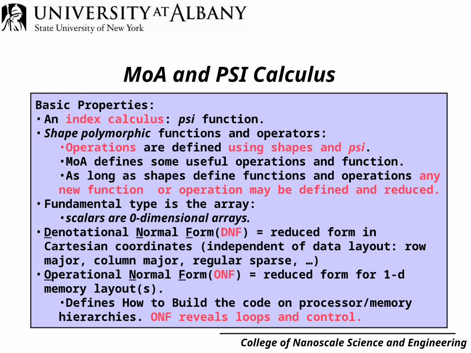
MoA and PSI CalculusBasic Properties:• An index calculus: psi function.• Shape polymorphic functions and operators:

•Operations are defined using shapes and psi.•MoA defines some useful operations and function.•As long as shapes define functions and operations any new function or operation may be defined and reduced.

• Fundamental type is the array:•scalars are 0-dimensional arrays.

• Denotational Normal Form(DNF) = reduced form in Cartesian coordinates (independent of data layout: row major, column major, regular sparse, …)

• Operational Normal Form(ONF) = reduced form for 1-d memory layout(s).

•Defines How to Build the code on processor/memory hierarchies. ONF reveals loops and control.


Historical Background

Universal Algebra – Joseph Sylvester, late 19th Century Algebra of Arrays - APL – Ken Iverson, 1950’s

• Languages: Interpreters

• Phil Abrams: An APL Machine(1972) with Harold Stone Indexing operations on shapes, open questions, not algebraic Indexing operations on shapes, open questions, not algebraic

closed system. Furthered by Hassett and Lyon, Guibas and closed system. Furthered by Hassett and Lyon, Guibas and Wyatt. Used in Fortran. Wyatt. Used in Fortran.

• Alan Perlis: Explored Abram’s optimizations in compilers for APL. Furthered by Miller, Minter, Budd. ZPL uses these ideas not full theory of arrays.

• Susan Gerhart: Anomalies in APL algebra, can not verify correctness.

• Alan Perlis with Tu: Array Calculator and Lambda Calculus mid 80’s.


Historical Background continued

MoA and Psi Calculus: Mullin 1988, full closure on Algebra of arrays and index calculus based on shapes. • Used with Lambda Calculus• Built prototype compilers: output C, F77, F90, HPF• Modified Portland Groups HPF, HPF Research Partner• Introduced Theory to Functional language Community

Bird-Meertens, SAC, …Bird-Meertens, SAC, …• Applied to Hardware Design and Verification

Pottinger(ASICS), IBM(Patent, Sparse Arrays), Sevaria(Hierarchical Pottinger(ASICS), IBM(Patent, Sparse Arrays), Sevaria(Hierarchical Bus Parallel Machines)Bus Parallel Machines)

• Introduce Theory to OO Community Expression Templates and C++, Optimizations for Scientific Expression Templates and C++, Optimizations for Scientific

Libraries, Matlab to VHDL optimizations(Sabbatical MIT Lincoln Libraries, Matlab to VHDL optimizations(Sabbatical MIT Lincoln Laboratory). Laboratory).


ApplicationsLevels of Processor/Memory Hierarchy

• Can be Modeled by Increasing Dimensionality of Data Array.

– Additional dimension for each level of the hierarchy.– Envision data as reshaped/transposed to reflect mapping to

increased dimensionality.– An Index Calculus automatically transforms algorithm to

reflect restructured data array.– Data, layout, data movement, and scalarization automatically

generated based on MoA descriptions and Psi Calculus Definitions of Array Operations, Functions and their compositions.

– Arrays are any dimension, even 0, I.e. scalars


Processor/Memory Hierarchycontinued

• Math and indexing operations in same expression

• Framework for design space search– Rigorous and provably correct– Extensible to complex architectures

Approach

Mathematics of Arrays

Example: “raising” arraydimensionality

y= convintricate math

intricatememory accesses(indexing)

(x)

Me

mo

ry H

iera

rch

y

Parallelism

Main Memory

L2 Cache

L1 Cache

Map

x: < 0 1 2 … 35 >

Map:

< 3 4 5 >< 0 1 2 >

< 6 7 8 >< 9 10 11 >

< 12 13 14 >

< 18 19 20 >< 21 22 23 >

< 24 25 26 >< 27 28 29 >

< 30 31 32 >

< 15 16 17 >

< 33 34 35 >

P0 P1 P2

P0

P1

P2


Application DomainSignal Processing3-d Radar Data Processing

Composition of Monolithic Array Operations

Algorithm is Input

Architectural Information is Input

Hardware Info:- Memory- Processor

Change algorithmto better match

hardware/memory/communication.Lift dimensionalgebraically

PulseCompression

DopplerFiltering

Beamforming Detection

Algebraically adding processors becomes 4-d, time 5-d,cache 6-d, Block-Cyclic decomposition requires restructuring

Algebraically adding processors becomes 4-d, time 5-d,cache 6-d, Block-Cyclic decomposition requires restructuring

Convolution Matrix Multiply


Manipulation of an array Given a 3 by 5 by 4 array:

Shape vector:

Index vector:

Used to select:

€

A =

0 1 2 3

4 5 6 7

8 9 10 11

12 13 14 15

16 17 18 19

⎡

⎣

⎢ ⎢ ⎢ ⎢ ⎢ ⎢

⎤

⎦

⎥ ⎥ ⎥ ⎥ ⎥ ⎥

,

€

20 21 22 23

24 25 26 27

28 29 30 31

32 33 34 35

36 37 38 39

⎡

⎣

⎢ ⎢ ⎢ ⎢ ⎢ ⎢

⎤

⎦

⎥ ⎥ ⎥ ⎥ ⎥ ⎥

,

€

40 41 42 43

44 45 46 47

48 49 50 51

52 53 54 55

56 57 58 59

⎡

⎣

⎢ ⎢ ⎢ ⎢ ⎢ ⎢

⎤

⎦

⎥ ⎥ ⎥ ⎥ ⎥ ⎥

€

ρA =< 354 >

€

i =< 213 >

€

iψA =< 213 >ψA = 47


Other Definitions Ravel: to flatten an array. Given B…

Now re-shape:€

B =

0 1 2 3 4

5 6 7 8 9

10 11 12 13 14

⎡

⎣

⎢ ⎢ ⎢

⎤

⎦

⎥ ⎥ ⎥

€

rav(B) =< 012 3456 789 10 1112 1314 >

€

< 5 3 > ρ rav(B) =

€

0 1 2

3 4 5

6 7 8

9 10 11

12 13 14

⎡

⎣

⎢ ⎢ ⎢ ⎢ ⎢ ⎢

⎤

⎦

⎥ ⎥ ⎥ ⎥ ⎥ ⎥


More Definitions

Reverse: Given an array

The reversal is given through indexing

Examples:

€

ξ

€

φξ

€

< i >ψ (φξ ) =< ρξ [0] − (i +1) >ψξ

€

rv =< 012 34 5 >

€

φ r

v =< 54 3210 >

€

ξ 2 =

0 1

2 3

4 5

6 7

⎡

⎣

⎢ ⎢ ⎢ ⎢

⎤

⎦

⎥ ⎥ ⎥ ⎥

€

φξ =

6 7

4 5

2 3

0 1

⎡

⎣

⎢ ⎢ ⎢ ⎢

⎤

⎦

⎥ ⎥ ⎥ ⎥


Some Psi Calculus OperationsBuilt Using ψ & Shapes

Operations

take

drop

rotate

cat

unaryOmega

binaryOmega

reshape

iota

Arguments

Vector A, int N

Vector A, int N

Vector A, int N

Vector A, Vector B

Operation Op, dimension D,Array A

Operation Op,Dimension Adim.Array A, Dimension Bdim,Array B

Vector A, Vector B

int N

Definition

Forms a Vector of the first N elements of A

Forms a Vector of the last (A.size-N) elements of A

Forms a Vector of the last N elements of A concatenated to the other elements of A

Forms a Vector that is the concatenation of A and B

Applies unary operator Op to D-dimensional components of A (like a for all loop)

Applies binary operator Op to Adim-dimensional components of A and Bdim-dimensional components of B (like a for all loop)

Reshapes B into an array having A.size dimensions, where the length in each dimension is given by the corresponding element of A

Forms a vector of size N, containing values 0 . . N-1

= index permutation = operators = restructuring = index generation


Psi Reduction

ONF has minimum number of reads/writes

PSI Calculus rules applied mechanically to produce ONF which is easily translated to optimal loop implementation

A=cat(rev(B), rev(C)) A[i]=B[size(B)-1-i] if 0≤ i < size(B)

A[i]=C[(size(C)+size(B))-1-i] if size(B) ≤ i <size(B)+size(C)


Psi Reduction: 2-d exampleDNF to ONF

Assume A, B, and C are n by n arrays.Let n=4.

C=(shift(A,1)+shift(B,2))T I. Get shape: shape((shift(A,1)+shift(B,2))T) = reverse(shape(shift(A,1)+shift(B,2)))= reverse(shape(shift(A,1))= reverse(shape(A)=reverse(n,n)=(n,n)

II Psi Reduce: for all I,j s.t. 0 <= I,j < (n,n)<I,j> psi (shift(A,1)+shift(B,2))T =<j,I> psi (shift(A,1)+shift(B,2)) =

(<j,I> psi shift(A,1)) + (<j,I> psi shift(B,2)) =(<I> psi (<j+1> psi A)) + (<I> psi (<j+2) psi B)) = DNFAvec[(gamma(j+1,n)*n)+iota(n)][I] + Bvec[(gamma(j+2,n)*n)+iota(n)][I] =Avec[(gamma(j+1,n)*n)+I] +Bvec[(gamma(j+2,n)*n)+I]=Avec[((j+1)*n)+I] + Bvec[((j+2)*n)+I] = ONF

Once we have the ONF we know how to build the code. Substituting when j=0 and I=0 above Avec[(1*4)+0] + Bvec[(2*4)+0] = Avec[4]+Bvec[8]

0 1 2 34 5 6 78 9 10 1112 13 14 15

0 1 2 34 5 6 78 9 10 1112 13 14 15

A= B=


New FFT algorithm: record speed

Maximize in-cache operations through use of repeated transpose-reshape operations

Similar to partitioning for parallel implementation

Do as many operations in cache as possible

Re-materialize the array to achieve locality

Continue processing in cache and repeat process


Example

Assume cache size c = 4; input vector length n = 32; number of rows r = n/c = 8

Generate vector of indices:

Use re-shape operator r to generate a matrix

€

rv = ι (n) =< 012K 31>


Starting Matrix

Each row is of length equal to the size “c”

Standard butterfly applied to each row as...

€

A ≡ rc ˆ ρ r v =

0 1 2 3

4 5 6 7

8 9 10 11

12 13 14 15

16 17 18 19

20 21 22 23

24 25 26 27

28 29 30 31

⎡

⎣

⎢ ⎢ ⎢ ⎢ ⎢ ⎢ ⎢ ⎢ ⎢ ⎢

⎤

⎦

⎥ ⎥ ⎥ ⎥ ⎥ ⎥ ⎥ ⎥ ⎥ ⎥


⎥⎥⎥⎥

⎦

⎤

⎢⎢⎢⎢

⎣

⎡

=

31272319151173

30262218141062

2925211713951

2824201612840

TA

Next transpose

To continue further would induce cache misses so transpose and reshape.

Transpose-reshape operation composed over indices (only result is materialized.

The transpose is:


Resulting Transpose-Reshape

Materialize the transpose-reshaped array B

Carry out butterfly operation on each row

Weights are re-ordered Access patterns are

standard...⎥⎥⎥⎥⎥⎥⎥⎥⎥⎥⎥

⎦

⎤

⎢⎢⎢⎢⎢⎢⎢⎢⎢⎢⎢

⎣

⎡

=≡

31272319

151173

30262218

141062

29252117

13951

28242016

12840

)(ˆ TArcB ρ


⎥⎥⎥⎥

⎦

⎤

⎢⎢⎢⎢

⎣

⎡

=

3115301429132812

27112610259248

237226215204

193182171160

TB

Transpose-Reshape again

As before: to proceed further would induce cache misses so:

Do the transpose-reshape again (composing indices) The transpose is:


⎥⎥⎥⎥⎥⎥⎥⎥⎥⎥⎥

⎦

⎤

⎢⎢⎢⎢⎢⎢⎢⎢⎢⎢⎢

⎣

⎡

=≡

31153014

29132812

27112610

259248

237226

215204

193182

71160

)(ˆ TBrcC ρ

Last step (in this example)

Materialize the composed transpose-reshaped array C

Carry out the last step of the FFT

This last step corresponds to cycles of length 2 involving elements 0 and 16, 1 and 17, etc.

1


Final Transpose Data has been permuted numerous times

• Multiple reshape-transposes We could reverse the transformations

• There would be multiple steps, multiple writes. Viewing the problem as an n-cube(hypercube for radix 2)

allows us to use the number of reshape-transposes as an argument to rotate(or shift) of a vector generated from the dimension of the hypercube.• This rotated vector is used as an argument to binary

transpose.• Permutes everything at once.• Express Algebraically, Psi reduce to DNF then ONF for a

generic design.• ONF has only two loops no matter what dimension

hypercube(or n-cube for radix = n) we start with.


Speed enhancement over previous record

0

0.5

1

1.5

2

2.5

3

3.5

4

4.5

5

1 2 3 4 5 6 7 8 9 10 11 12 13 14 15 16 17 18 19 20 21 22

Log_2(size of FFT)

Enhancement Ratio


FFT Time vs. size

0.0001

0.001

0.01

0.1

1

10

100

1 2 3 4 5 6 7 8 9 10 11 12 13 14 15 16 17 18 19 20 21 22

log_2(FFT size)

Time (sec)

optimized

not optimized


Summary All operations have been carried out in cache at the

price of re-arranging the data Data blocks can be of any size (powers of the radix):

need not equal the cache size Optimum performance: tradeoff between reduction of

cache misses and cost of transpose-reshape operations Number of transpose-reshape operations determined

by the data block size (cache size) Record performance: up to factor of 4 better than

libraries


Benefits of Using MOA and Psi Calculus

Processor/Memory Hierarchy can be modeled by reshaping data using an extra dimension for each level.

Composition of monolithic operations can be reexpressed as composition of operations on smaller data granularities

• Matches memory hierarchy levels• Avoids materialization of intermediate arrays.

Algorithm can be automatically(algebraically) transformed to reflect array reshapings above.

Facilitates programming expressed at a high level• Facilitates intentional program design and analysis• Facilitates portability

This approach is applicable to array-based computation in general.


Current Research Using MoA and Psi Calculus to Describe Abstract

Processor/Memory Hierarchies and Instruction Sets. Working with Library Developers to Mechanize some or all of the

MoA algebra with the Psi Calculus.

• Andrew Lumsdaine, Matrix Template Library, etc.

• Bob Bond, Expression Templates to Optimize Scientific Libraries, explore connection to Matlab to VHDL.

Developing Designs for Hardware

• Indentify how to easily Program and Optimize FPGAs in conjunction with new machines and their cooperative OSs, e.g. Cray XD1.

• FFT presently is radix n, m-dimensional, supports a cache loop, and is across multiple processors both shared and distributed.

• QR, TD Convolution, LU, Matrix Multiple(inner product), Kronecker Product(outer product) have been previously designed and include processor/cache loops.


Current Research continued

Identifying bottlenecks in first-principles scientific simulations: FFT (PDE solvers have similar memory accesses).

• Such problems are the large grid problems that require deterministic resource allocation. High-speed and huge data sizes are essential. Real-time is the goal.

• Scientific Simulations include: Weather, Materials Deposition, Earthquake prediction, Oil Location, Ground Water Contamination, etc. All require the same algorithms.

Monograph documenting theory and applications.• DSP Journal, comprehensive introduction to both.(to

appear)• Continue to teach and assist those who may benefit.

Documents

College of Nanoscale Science and Engineering The application of Conformal Computing techniques to problems in computational physics: The Fast Fourier Transform