Embed Size (px)
Citation preview

College Algebra(Draft)
by Avinash Sathaye, Professor of Mathematics
Department of Mathematics, University of Kentucky
D(4,–3):Quad 4
B(–4,3):Quad 2 A(4,3):Quad 1
C(–4,–3):Quad 3 –3
–2
–1
1
2
3
–10 –5 5 10
July 27, 2005

2
Contents
1 Polynomials, the building blocks of algebra 11.1 Underlying field of numbers. . . . . . . . . . . . . . . . . . . . . . . . 11.2 Indeterminates, variables, parameters . . . . . . . . . . . . . . . . . . 21.3 Basics of Polynomials . . . . . . . . . . . . . . . . . . . . . . . . . . . 31.4 Working with polynomials . . . . . . . . . . . . . . . . . . . . . . . . 61.5 Examples of polynomial operations. . . . . . . . . . . . . . . . . . . . 8
Example 1. Polynomial operations. . . . . . . . . . . . . . . . . . . 8Example 2. Collecting coefficients. . . . . . . . . . . . . . . . . . . . 9Example 3. Using algebra for arithmetic. . . . . . . . . . . . . . . . 9Example 4. Expanding powers. . . . . . . . . . . . . . . . . . . . . 10Example 5. Substituting in a polynomial. . . . . . . . . . . . . . . . 11Example 6. Completing the square. . . . . . . . . . . . . . . . . . . 12
2 Solving linear equations. 152.0.1 What is a solution? . . . . . . . . . . . . . . . . . . . . . . . . 16
2.1 One linear equation in one variable. . . . . . . . . . . . . . . . . . . . 162.2 Several linear equations in one variable. . . . . . . . . . . . . . . . . . 182.3 Two or more equations in two variables. . . . . . . . . . . . . . . . . 182.4 Several equations in several variables. . . . . . . . . . . . . . . . . . . 192.5 Solving linear equations efficiently. . . . . . . . . . . . . . . . . . . . 20
Example 1. Manipulation of equations. . . . . . . . . . . . . . . . . 20Example 2. Cramer’s Rule. . . . . . . . . . . . . . . . . . . . . . . . 21Example 3. Exceptions to Cramer’s Rule. . . . . . . . . . . . . . . . 22Example 4. Cramer’s Rule with many variables. . . . . . . . . . . . 23
3 The division algorithm and applications 273.1 Repeated Division. . . . . . . . . . . . . . . . . . . . . . . . . . . . . 303.2 The GCD and LCM of two polynomials: meaning and calculations. . 313.3 Aryabhata algorithm: Efficient Euclidean algorithm. . . . . . . . . . . 32
Example 1. Kuttaka or Chinese Remainder Theorem.. . . . . . . . . 353.4 Division algorithm in integers. . . . . . . . . . . . . . . . . . . . . . . 38
Example 2. GCD calculation in Integers. . . . . . . . . . . . . . . . 40
3

4 CONTENTS
Example 3. Efficient division by a linear polynomial. . . . . . . . . . 42
Example 4. Division by a quadratic polynomial. . . . . . . . . . . . 44
4 Introduction to analytic geometry. 49
4.1 Coordinate systems. . . . . . . . . . . . . . . . . . . . . . . . . . . . 49
4.2 Geometry: Distance formulas. . . . . . . . . . . . . . . . . . . . . . . 50
4.3 Change of coordinates on a line. . . . . . . . . . . . . . . . . . . . . . 52
4.4 Change of coordinates in the plane. . . . . . . . . . . . . . . . . . . . 53
4.5 General change of coordinates: . . . . . . . . . . . . . . . . . . . . . . 54
Examples. Changes of coordinates. . . . . . . . . . . . . . . . . . . 55
5 Equations of lines in the plane. 59
Examples. Parametric equations of lines. . . . . . . . . . . . . . . . 59
5.1 Meaning of the parameter t: . . . . . . . . . . . . . . . . . . . . . . . 61
Examples. Special points on parametric lines. . . . . . . . . . . . . . 62
5.2 Details of the equation of a line. . . . . . . . . . . . . . . . . . . . . . 64
5.3 Examples of equations of lines. . . . . . . . . . . . . . . . . . . . . . . 68
Example 1. Points equidistant from two given points. . . . . . . . . 68
Example 2. Right angle triangles. . . . . . . . . . . . . . . . . . . . 69
6 The Circle 71
6.1 Parametric form of a circle. . . . . . . . . . . . . . . . . . . . . . . . 72
6.2 Trigonometric parametrization. . . . . . . . . . . . . . . . . . . . . . 73
Definition. Trigonometric Functions. . . . . . . . . . . . . . . . . . . 75
6.2.1 Yet another take on parametrizing the circle. . . . . . . . . . . 79
Pythagorean Triples. Generation of. . . . . . . . . . . . . . . . . . 79
6.3 Examples of equations of a circle. . . . . . . . . . . . . . . . . . . . . 82
Example 1. Intersection of two circles. . . . . . . . . . . . . . . . . . 82
Example 2. Line joining through the intersection of two circles. . . . 83
Example 3. Circle through three given points. . . . . . . . . . . . . 83
Example 4. Exceptions to a circle through three points. . . . . . . . 84
Example 5. Smallest circle with a given center meeting a given line. 84
Example 6. The distance between a point and a line. . . . . . . . . 85
Example 7. Half plane defined by a line. . . . . . . . . . . . . . . . 86
7 Special study of Linear and Quadratic Polynomials. 89
7.1 Linear Polynomials. . . . . . . . . . . . . . . . . . . . . . . . . . . . 89
7.2 Factored Quadratic Polynomial. . . . . . . . . . . . . . . . . . . . . 90
Interval notation. Intervals on real line. . . . . . . . . . . . . . . . 90
7.3 The General Quadratic Polynomial. . . . . . . . . . . . . . . . . . . . 91
7.4 Examples of quadratic polynomials. . . . . . . . . . . . . . . . . . . . 93

CONTENTS 5
8 Functions 958.1 Plane algebraic curves . . . . . . . . . . . . . . . . . . . . . . . . . . 958.2 What is a function? . . . . . . . . . . . . . . . . . . . . . . . . . . . . 968.3 Modeling a function. . . . . . . . . . . . . . . . . . . . . . . . . . . . 97
9 Looking closely at a function 101Parabola. Analysis near its points. . . . . . . . . . . . . . . . . . . . 101Circle. Analysis near its points. . . . . . . . . . . . . . . . . . . . . . 104
9.1 Analyzing a general curve y = f(x) near a point (a, f(a)). . . . . . . 1059.2 The slope of the tangent, calculation of the derivative. . . . . . . . . 1079.3 Derivatives of more complicated functions. . . . . . . . . . . . . . . . 1109.4 More complicated derivatives. . . . . . . . . . . . . . . . . . . . . . . 1119.5 Using the derivatives for approximation. . . . . . . . . . . . . . . . . 114
Linear Approximation. Examples. . . . . . . . . . . . . . . . . . . 1149.6 Efficient expansions of polynomials, the Binomial Theorem. . . . . . . 116
10 Root finding 11910.1 Newton’s Method . . . . . . . . . . . . . . . . . . . . . . . . . . . . . 11910.2 Limitations of the Newton’s Method . . . . . . . . . . . . . . . . . . 121
11 Summation of series. 12511.1 Application of polynomials . . . . . . . . . . . . . . . . . . . . . . . . 12511.2 Examples of summation of series. . . . . . . . . . . . . . . . . . . . . 126
12 More on the Trigonometric Functions. 12912.1 Basic definitions of Trigonometric Functions. . . . . . . . . . . . . . . 12912.2 Connection with the usual Trigonometric Functions. . . . . . . . . . . 13112.3 Addition Formula. . . . . . . . . . . . . . . . . . . . . . . . . . . . . 13212.4 Identities Galore. . . . . . . . . . . . . . . . . . . . . . . . . . . . . . 13412.5 Using trigonometry. . . . . . . . . . . . . . . . . . . . . . . . . . . . . 139
Index . . . . . . . . . . . . . . . . . . . . . . . . . . . . . . . . . . . . . . . . . . . . . . . . . . . . . . . . . . . . . . . . . . . . . . . . . . . . 143

6 CONTENTS
Introduction.
This book on College Algebra is designed with a different philosophy from the othertextbooks on the same subject.
The core material of a course on College Algebra is usually a subset of therecommended material expected to be taught in a high school course. The materialis usually taught at a slow pace with extensive practice and lots of routine exercises.The College Algebra course usually attempts to get the student prepared forextensive calculations using a calculator and discusses several real life examples formotivation as well as practice. Due to short amount of time available and manyspecific topics to study, the students end up learning how to answer specificquestions.
Often there is not enough time or motivation to get an overall view of any specificsubject and due to the emphasis on solving specific practical problems with explicitdecimal answers, the student has no time or motivation to study how the answersare derived. A typical student often insists that ”don’t tell me too many ways ofdoing something; don’t tell me how the formula is derived; just show me how to dothe problems which will appear on the test!”.
When a trained student goes to a higher level course, he still needs such an explicithelp, since he has not learned how to create his own theory and set up his ownequations.
Our hope is to offer a course where the emphasis is on mastering the Algebraictechnique. Algebra consists of manipulating expressions to put them in convenientform for getting at desired answers. Algebra consists of looking for ways of findinginformation about various quantities even though it is difficult to actually solve forthem. Algebra consists of
finding multiple expressions for the same quantities, for the comparison of differentexpressions often leads to new discoveries.
We urge the readers to approach this book with an open mind. You may find newperspective on known topics.
We urge the reader to carefully study and memorize the definitions. A majority ofmistakes are caused by forgetting what a certain term means.
We urge the reader to be bold. Don’t be afraid of a long involved calculation.Answers which pop out in a step or two hide the true meaning of what is going on.As far as possible, try to do the derivations yourself. If you get stuck, look up orask. The derivations are not to be memorized, they should be done as a freshexercise in Algebra; a regular exercise is good for you!
We urge the reader to be inquisitive. Don’t take anything for granted, until youunderstand it. Don’t be ever satisfied by a single way of doing things; look foralternative shortcuts.
We also urge the reader to be creatively lazy. Look for simpler (yet correct, ofcourse) ways of doing the same calculations. If there is a string of numerical
CONTENTS 7
calculations, don’t just do them. Try to build a formula of your own; perhapssomething that you could then feed into a computer some day.A warning about graphing. Graphs are a big help in understanding the problem andthey help you set up the right questions. They are also notorious in misleading youinto wrong configurations or suggesting possible wrong answers. Never trust ananswer until it is verified by theory or straight calculations.Calculators are useful for getting answers but in this course, most questions aredesigned for precise algebraic answers. A computer system which is capable ofinfinite precision calculations can be used for study and is recommended. But makesure that you understand the calculations well.
What is Algebra?
Algebra is the part of mathematics dealing with manipulation of expressions andsolutions of equations. Since these operations are needed in all branches ofmathematics, algebraic skill is a fundamental need for doing mathematics.The name algebra itself is a shortened form of the title of an old Arabic book onalgebra entitled al jabr wa al mukabala which roughly means manipulation (ofexpressions) and comparison (of equations).It is the foundation and the core of higher mathematics. A strong foundation inAlgebra will help students to become better mathematicians, analyzers, andthinkers.The fundamental operations of algebra are addition, subtraction, multiplication anddivision (except by zero). An extended operation derived from the idea of repeatedmultiplication is the exponentiation (raising to a power).We start Algebra with the introduction of variables. Variables are simply symbolsused to represent unknown quantities. Next we combine these variables intomathematical expressions using algebraic operations and numbers. In other words,we learn to handle them just like numbers. The real power of Algebra comes inwhen we learn tools and techniques to solve equations involving various kinds ofexpressions for appropriate values.Often, the expected solutions are just numbers, but at higher levels, we need todevelop a finer idea of what we can accept as a solution. This equation solving isthe art of Algebra! 1
1Here is thought for the philosophical readers. Think what you mean when you say that√
2 is asolution to the equation x2 − 2. Do we really have an independent evidence that
√2 makes sense,
other than saying that it has square equal to 2? And is it not just an alternate way of saying thatit is a solution of the desired equation? Now having thought of a name
√2 for the answer, we can
proceed to compare it with other known numbers, find various decimal digits of its expansion andso on.
In higher mathematics, we find a way of turning this abstract thought into solutions of equationsby declarations and into the art of finding the properties of solutions of equations without ever

8 CONTENTS
A student in a College Algebra course is expected to be familiar with suchoperations and sufficiently skilled in performing them with ease and speed. The firsthomework and diagnostic test will help evaluate the level of these skills.We next discuss a few generalities which will be useful for a general understanding.If things begin to become frustrating, remember that learning Algebra is much likelearning a new language.It is important to first have all the letters, sounds, words, and punctuation downbefore you can make a correct sentence, or in our case, write and solve an equation.Of course, there are people who can pick up a language without ever learninggrammar, by being good at imitating others and picking up on what is important.You may be one of these few lucky ones, but be sure to verify your feeling with thecorrect rules. Unlike a spoken language, mathematics has a very precise structure!
solving them! You will see some examples of this later.

CONTENTS 1

2 CONTENTS

Chapter 1
Polynomials, the building blocks ofalgebra
1.1 Underlying field of numbers.
To begin our work in Algebra, we must first each use the same notations tocommunicate. Mathematicians do this by agreeing to a field of numbers to work in.In our field we will want numbers which allow all of the four basic operations:addition, subtraction, multiplication, and division (except by 0). For our purpose,we usually include the set of all real numbers denoted by <.
The set of rational numbers consists of all numbers of the form ±a/b where a, bare non negative integers with a non zero b. It is denoted by Q . A more familiar setfor you is probably < the set of real numbers which may be thought of as the setof all possible decimal numbers (with expansions of unlimited length).You might have already seen that a rational number may be expressed as a finitedecimal (for example 3
4= 0.75 or a repeating decimal 4
3= 1.3333 ) 1
In a slightly more advanced setting you may find the set of complex numbers C .It is obtained from < by throwing in one extra number denoted as i. This number iis defined by the basic equation i2 = −1. By the known algebraic operations, it iseasy to see that every number of the form u + iv where u, v are real numbers mustbe in C . Conversely, it is not hard to convince yourself that all the four algebraicoperations on numbers of the form u + iv result in numbers of the same form. 2
In your higher level math classes you will also encounter the set of complex numbersdenoted by C . However, we will use the complex numbers only on special occasions.
1Recall that the line over 3 indicates the digit 3 repeated indefinitely.2An enthusiastic reader only needs to verify the formulas:
(a + ib)(c + id) = (ac − bd) + i(ad + bc) and 1/(a + ib) = a/(a2 + b2) − bi/(a2 + b2).
It is easy to see that now all algebraic operations can be easily performed.To verify your understanding, assign yourself the task of verifying the following:
1
2 CHAPTER 1. POLYNOMIALS, THE BUILDING BLOCKS OF ALGEBRA
We may, occasionally, denote our set of underlying numbers by the letter F (toremind us of its technical mathematical term - a field). Usually, we may just callthem numbers and we will usually be talking about the field of real numbers i.e.F = <.
1.2 Indeterminates, variables, parameters
If you see an expression like ax2 + bx + c; you usually think of this as an expressionin a variable x with constants a, b, c.
At this stage, x as well as a, b, c are unspecified. However, we are assuming thata, b, c are fixed while x is a variable which may be pinned down after some extrainformation - for example, if the expression is set equal to zero.
Thus, in algebraic expressions, the idea of who is constant and who is a variable is amatter of declaration or convention.
Variables
As you may recall from Chapter 1, a variable is a symbol, typically a Greek orStandard English letter, used to represent an unknown quantity. However, not allsymbols are variables and it is typically a matter of declaration in order to decipherwhich is a variable and which is a constant.
Take this familiar expression for example:
mx + c.
You may already remember seeing this in connection with the equation of a line.
Recall that m in mx + c used to be a constant and not a variable. The letter m wasthe slope of a certain line and was a fixed number when we knew the line.
The letter c in mx + c also used to be a constant. It used to be the y-intercept (i.e.the y-coordinate of the intersection of the line and the y-axis).
The x in mx + c is the variable in this expression and represents a changing value ofthe x-coordinate. The expression mx + c then gives the y-coordinate of thecorresponding point on the line.
Parameters
Certain variables are often called parameters; here the idea is that a parameteris avariable which is not intended to be pinned down to a specific value, but is expectedto move thru a preassigned set of values generating interesting quantities. In otherwords, a parameter is to be thought of as unspecified constant in a certain range ofvalues.
1
1 + i=
1 − i
2, (−1 ±
√3i)3 = 8 , (1 + i)4 = −4.

1.3. BASICS OF POLYNOMIALS 3
In the above example of mx + c we may think of m, c as parameters. They canchange, but once a line is pinned down, they are fixed. Then only the x stays avariable.
As another example, let 1 + 2t be the distance of a particle from a starting positionat time t, then t might be thought of as a parameter describing the motion of theparticle. It is pinned down as soon as we locate the moving point.
The same t can also be simply called a variable if we start asking a question like“At what time is the distance equal to 5?”.
Then we will write an equation 1 + 2t = 5 and by algebraic manipulation, declarethat t = 2.
Indeterminates
An indeterminate usually is a symbol which is not intended to be substituted withvalues; thus it is like a variable in appearance, but we don’t care to assign or changevalues for it. Thus the statement
X2 − a2 = (X − a)(X + a)
is a formal statement about expansion and X, a can be thought of as indeterminates.
When we use it to factor y2 − 9 as (y − 3)(y + 3) we are turning X, a into variablesand substituting values y, 3 to them! 3
1.3 Basics of Polynomials
We now can now show how polynomials are constructed and handled. This materialis very important for success in Algebra.
Monomials
The basic definition of a monomial is this:
• Given a variable x and a constant a, let n be a non negative integer. Then anexpression of the form axn is said to be a monomial.
• The constant a is said to be its coefficient.(Sometimes we call it thecoefficient of xn).
• The degree of the monomial is said to be n.
• Sometimes, we need monomials with more general exponents, meaningwe allow n to be a negative integer as well. The rest of the definition is thesame. We will always make it clear if we are using such general exponents.
3In short, the distinction between an indeterminate, variable and parameter, is, like beauty, inthe eye of the beholder!

4 CHAPTER 1. POLYNOMIALS, THE BUILDING BLOCKS OF ALGEBRA
For example, consider the monomial 4x3. Its variable is x, its coefficient is 4 and itsdegree is 3.This basic definition can be made fancier as needed.Usually, n is an integer, but in higher mathematics, n can be a more general object.
As already stated, we can accept − 52x3 = (−5/2)x−3 as an acceptable monomial
with general exponents. We declare that its variable is x and it has degree −3with coefficient −5/2.Notice that we collected all parts (including the minus sign) of the expression exceptthe power of x to build the coefficient!
Monomials in several variables.It is permissible to use more than one variables and write a monomial of the formaxpyq. This is a monomial in x, y with coefficient a. Its degree is said to be p + q.Its exponents are said to be (p, q) respectively (with respect to variables x, y). Asbefore, more general exponents may be allowed, if necessary. 4
Example.Consider this example of a monomial in x,y.
21x3y4
−3xy.
What are the exponents, degree etc.? First, we must simplify the expression to:
−7x2y3.
Thus its coefficient is −7, its degree is 2 + 3 = 5 and the exponents are (2, 3).What happens if we change our idea of who the variables are?Consider the same simplified monomial −7x2y3.Let us think of it as a monomial in y. Then we rewrite it as:
(−7x2)y3.
Thus as a monomial in y alone, its coefficient is −7x2 and its degree is 3.What happens if we take the same monomial −7x2y3 and make x as ourvariable?Then we rewrite it as:
(−7y3)x2.
Be sure to note the rearrangement!Thus as a monomial in x alone, its coefficient is −7y3 and its degree is 2.
4For the reader who likes formalism, here is a general definition. A monomial in variablesx1, · · · , xr is an expression of the form axn1 · · ·xnr where n1, · · · , nr are non negative integers and ais any expression which is free of the variables x1, · · · , xr. The coefficient of the monomial is a, thedegree is n1 + · · · + nr and the exponents are said to be n1, · · · , nr.
In higher mathematics, n1, · · · , nr may be allowed to be more general.
1.3. BASICS OF POLYNOMIALS 5
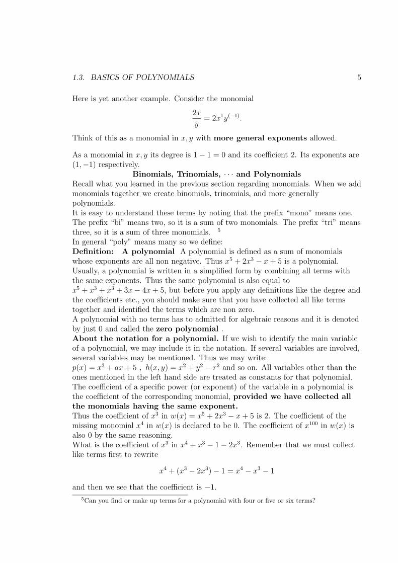
Here is yet another example. Consider the monomial
2x
y= 2x1y(−1).
Think of this as a monomial in x, y with more general exponents allowed.
As a monomial in x, y its degree is 1 − 1 = 0 and its coefficient 2. Its exponents are(1,−1) respectively.
Binomials, Trinomials, · · · and PolynomialsRecall what you learned in the previous section regarding monomials. When we addmonomials together we create binomials, trinomials, and more generallypolynomials.It is easy to understand these terms by noting that the prefix “mono” means one.The prefix “bi” means two, so it is a sum of two monomials. The prefix “tri” meansthree, so it is a sum of three monomials. 5
In general “poly” means many so we define:Definition: A polynomial A polynomial is defined as a sum of monomialswhose exponents are all non negative. Thus x5 + 2x3 − x + 5 is a polynomial.Usually, a polynomial is written in a simplified form by combining all terms withthe same exponents. Thus the same polynomial is also equal tox5 + x3 + x3 + 3x − 4x + 5, but before you apply any definitions like the degree andthe coefficients etc., you should make sure that you have collected all like termstogether and identified the terms which are non zero.A polynomial with no terms has to admitted for algebraic reasons and it is denotedby just 0 and called the zero polynomial .About the notation for a polynomial. If we wish to identify the main variableof a polynomial, we may include it in the notation. If several variables are involved,several variables may be mentioned. Thus we may write:p(x) = x3 + ax + 5 , h(x, y) = x2 + y2 − r2 and so on. All variables other than theones mentioned in the left hand side are treated as constants for that polynomial.The coefficient of a specific power (or exponent) of the variable in a polynomial isthe coefficient of the corresponding monomial, provided we have collected allthe monomials having the same exponent.Thus the coefficient of x3 in w(x) = x5 + 2x3 − x + 5 is 2. The coefficient of themissing monomial x4 in w(x) is declared to be 0. The coefficient of x100 in w(x) isalso 0 by the same reasoning.What is the coefficient of x3 in x4 + x3 − 1 − 2x3. Remember that we must collectlike terms first to rewrite
x4 + (x3 − 2x3) − 1 = x4 − x3 − 1
and then we see that the coefficient is −1.
5Can you find or make up terms for a polynomial with four or five or six terms?

6 CHAPTER 1. POLYNOMIALS, THE BUILDING BLOCKS OF ALGEBRA
1.4 Working with polynomials
Given several polynomials, we can perform the usual operations of addition,subtraction and multiplication on them. We can also do division, but if we expectthe answer to be a polynomial again, then we have a problem. We will discuss thesematters later. 6
As a simple example, let f(x) = 3x5 + x, g(x) = 2x5 − 2x2, h(x) = 3, w(x) = 2.Then f(x) + g(x) = 3x5 + x + 2x5 − 2x2 and we need to collect like terms to writethe answer as f(x) + g(x) = 5x5 − 2x2 + x. Notice that we have also arranged themonomials in decreasing degrees, this is a recommended practice for polynomials.What is w(x)f(x) − h(x)g(x)? We see that
(2)(3x5 + x) − (3)(2x5 − 2x2) = 6x5 + 2x − 6x5 + 6x2 = 6x2 + 2x.
Definition: Degree of a polynomial with respect to a variable x is defined to bethe highest degree of any monomial present in the polynomial (i.e. any monomialaxm with a 6= 0 in the polynomial). We shall write degx(p) for the degree of p withrespect to x. The degree of a zero polynomial is defined differently by differentpeople. Some declare it not to have a degree, other take it as −1 and yet others takeit as −∞. We shall declare it undefined and hence we always have to be careful todetermine if our polynomial reduces to 0.We also have use for Definition: Leading coefficient of a polynomial For apolynomial p(x) with degree n in x, by its leading coefficient, we mean thecoefficient of xn in the polynomial.Thus given a polynomial x3 + 2x5 − x − 1 we first rewrite it as 2x5 + x3 − x − 1 andthen we can say that its degree is 5, and its leading coefficient is 2.The following are some of the evident facts about polynomials and their degrees.Assume that u = axn + · · · , v = bxm + · · · are non zero polynomials in x ofdegrees n, m respectively.We shall need the following useful facts.
1. Note that by saying that u has degree n we are announcing that the coefficienta of xn is non zero and that none of the other (monomial) terms has degree ashigh as n.
Similarly, by saying that v has degree m, we mean that b 6= 0 and no otherterms in v are of degree as high as m.
2. For a non zero number c we have that cu has the same degree as u and indeedits leading coefficient is ca.
6The situation is similar to integers. If we wish to divide 7 by 2 then we get a rational number72 which is not an integer any more. It is fine if you are willing to work with the rational numbers.You might have also seen the idea of division with remainder which says divide 7 and 2 and you geta division of 3 and a remainder of 1, i.e. 7 = (2)(3) + 1.
As promised, we shall take this up later.

1.4. WORKING WITH POLYNOMIALS 7
For example, if c is a constant, then the degree of c(2x5 + x − 2) is always 5,except when c = 0. For c = 0 it becomes undefined! Note that for non zero c,the leading coefficient of cu is simply ca.
3. Suppose that the degrees n, m of u, v are unequal. Then for non zeroconstants c, d we can decide the degree of cu + dv to be the maximum of n, m.It is easy to figure out the degree if one or more of c, d have special values.
For example, if u = 2x5 + x − 2 and v = −x3 + 3x − 1, then the degree ofcu + dv is calculated thus:
cu+dv = c(2x5+x−2)+d(−x3+3x−1) = (2c)x5+(−d)x3+(c+3d)x+(−2c−d)
Thus, the degree will be 5 as long as c 6= 0. It will drop to 3 if c = 0 but d 6= 0.If c, d are both zero then it becomes undefined. It is useful to understand thisusing concrete values of c, d.
The reader should verify that the leading coefficients are respectively, 2c or −dor undefined.
4. Let c, d be non zero numbers and consider h = cu + dv. If the degrees of u, vare the same, i.e. n = m then the degree of h is not so easy to tell withoutcareful analysis.
However, we can at least say that
• Either h = 0 and hence degx(h) is undefined, or
• 0 ≤ degx(h) ≤ n = m.
For example, let u = −x3 + 3x2 + x − 1 and v = x3 − 3x2 + 2x − 2. Calculatecu + dv with c, d constants.
cu + dv = c(−x3 + 3x2 + x − 1) + d(x3 − 3x2 + 2x − 2)= (−c + d)x3 + (3c − 3d)x2 + (c + 2d)x + (−c − 2d)
We determine the degree of the expression thus:
• If −c + d 6= 0, i.e. c 6= d then the degree is 3.
• If c = d, the the x2 term also vanishes and we get
cu + dv = (c + 2d)x + (−c − 2d) = (3d)x + (−3d).
Thus if d = 0 then the degree is undefined and if d 6= 0 then the degree is1.

8 CHAPTER 1. POLYNOMIALS, THE BUILDING BLOCKS OF ALGEBRA
The reader is encouraged to figure out the formula for the leading coefficientsin each case.
The reader should also experiment with other polynomials.
5. The product rule for degrees. The degree of the product of two non zeropolynomials is always the sum of their degrees. This means:
degx(uv) = degx(u) + degx(v) = m + n.
Indeed, we can see that
uv = (axn + terms of degree less than n )(bxm + terms of degree less than m )= (ab)x(m+n) + terms of degree less than m + n .
Thus the leading coefficient of the product is ab, i.e. the product of theirleading coefficients.
1.5 Examples of polynomial operations.
• Example 1: Consider p(x) = x3 + x + 1 and q(x) = −x3 + 3x2 + 5x + 5. Whatare their degrees?
Also, calculate the following expressions:
p(x) + q(x) , p(x) + 2q(x) and p(x)2.
Answers: The degrees of p(x), q(x) are both 3. The remaining answers are:
p(x) + q(x) = x3(1 − 1) + x2(0 + 3) + x(1 + 5) + (1 + 5)= 3x2 + 6x + 6
p(x) + 2q(x) = x3(1 − 2) + x2(0 + 6) + x(1 + 10) + (1 + 10)= −x3 + 6x2 + 11x + 11
(x3 + x + 1)(x3 + x + 1) = (x6 + x4 + x3) + (x4 + x2 + x) + (x3 + x + 1)= x6 + 2x4 + 2x3 + x2 + 2x + 1
Here is an alternate technique for the last answer. It will be useful for futurework.
First, note that the degree of the answer is 3 + 3 = 6 from the product ruleabove. Thus we need to calculate coefficients of all powers xi for i = 0 to i = 6.
Each xi term comes from multiplying an xj term and an xi−j term from p(x).Naturally, both j and i − j need to be between 0 and 3.
1.5. EXAMPLES OF POLYNOMIAL OPERATIONS. 9
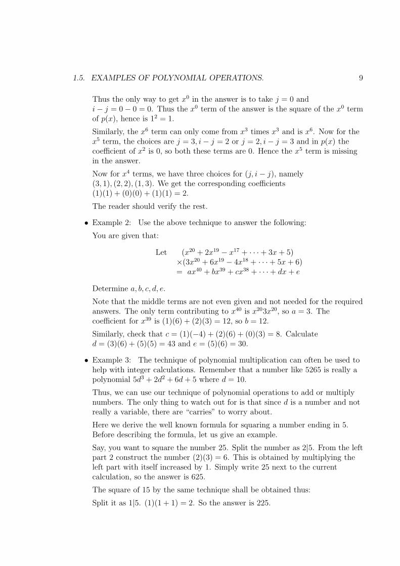
Thus the only way to get x0 in the answer is to take j = 0 andi − j = 0 − 0 = 0. Thus the x0 term of the answer is the square of the x0 termof p(x), hence is 12 = 1.
Similarly, the x6 term can only come from x3 times x3 and is x6. Now for thex5 term, the choices are j = 3, i − j = 2 or j = 2, i − j = 3 and in p(x) thecoefficient of x2 is 0, so both these terms are 0. Hence the x5 term is missingin the answer.
Now for x4 terms, we have three choices for (j, i − j), namely(3, 1), (2, 2), (1, 3). We get the corresponding coefficients(1)(1) + (0)(0) + (1)(1) = 2.
The reader should verify the rest.
• Example 2: Use the above technique to answer the following:
You are given that:
Let (x20 + 2x19 − x17 + · · · + 3x + 5)×(3x20 + 6x19 − 4x18 + · · ·+ 5x + 6)= ax40 + bx39 + cx38 + · · ·+ dx + e
Determine a, b, c, d, e.
Note that the middle terms are not even given and not needed for the requiredanswers. The only term contributing to x40 is x203x20, so a = 3. Thecoefficient for x39 is (1)(6) + (2)(3) = 12, so b = 12.
Similarly, check that c = (1)(−4) + (2)(6) + (0)(3) = 8. Calculated = (3)(6) + (5)(5) = 43 and e = (5)(6) = 30.
• Example 3: The technique of polynomial multiplication can often be used tohelp with integer calculations. Remember that a number like 5265 is really apolynomial 5d3 + 2d2 + 6d + 5 where d = 10.
Thus, we can use our technique of polynomial operations to add or multiplynumbers. The only thing to watch out for is that since d is a number and notreally a variable, there are “carries” to worry about.
Here we derive the well known formula for squaring a number ending in 5.Before describing the formula, let us give an example.
Say, you want to square the number 25. Split the number as 2|5. From the leftpart 2 construct the number (2)(3) = 6. This is obtained by multiplying theleft part with itself increased by 1. Simply write 25 next to the currentcalculation, so the answer is 625.
The square of 15 by the same technique shall be obtained thus:
Split it as 1|5. (1)(1 + 1) = 2. So the answer is 225.
10 CHAPTER 1. POLYNOMIALS, THE BUILDING BLOCKS OF ALGEBRA
The general rule is this:
Let a number n be written as p5 where p is the part of the number after theunits digit 5.
Then n2 = (p)(p + 1)25, i.e. (p)(p + 1) becomes the part of the number fromthe 100s digit onwards.
To illustrate, consider 452. Here p = 4, so (p)(p + 1) = (4)(5) = 20 and so theanswer is 2025. Also 1052 = (10)(11)25 = 11025. Similarly52652 = (526)(527)25, i.e. 27720225.
What is the proof? Our n = pd + 5, so
n2 = (pd + 5)(pd + 5)= p2d2 + (2)(5)(pd) + 25= p2(100) + p(100) + 25= (p2 + p)100 + 25.
Thus the part after the 100s digits is p2 + p = p(p + 1).
You can use such techniques for developing fast calculation methods.
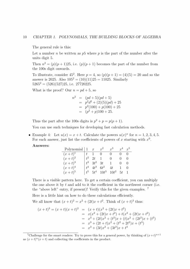
• Example 4: Let u(x) = x + t. Calculate the powers u(x)n for n = 1, 2, 3, 4, 5.For each answer, just list the coefficients of powers of x starting with x0.
Answers:Polynomial 1 x x2 x3 x4 x5
(x + t)1 t 1 0 0 0 0(x + t)2 t2 2t 1 0 0 0(x + t)3 t3 3t2 3t 1 0 0(x + t)4 t4 4t3 6t2 4t 1 0(x + t)5 t5 5t4 10t3 10t2 5t 1
There is a visible pattern here. To get a certain coefficient, you can multiplythe one above it by t and add to it the coefficient in the northwest corner (i.e.the “above left” entry, if present)! Verify this for the given examples. 7
Here is a little hint on how to do these calculations efficiently.
We all know that (x + t)2 = x2 + (2t)x + t2. Think of (x + t)3 thus:
(x + t)3 = (x + t)(x + t)2 = (x + t)(x2 + (2t)x + t2)= x(x2 + (2t)x + t2) + t(x2 + (2t)x + t2)= x3 + (2t)x2 + (t2)x + (t)x2 + (2t2)x + (t3)= x3 + (2t + t)x2 + (t2 + 2t2)x + (t3)= x3 + (3t)x2 + (3t2)x + t3
7Challenge for the smart readers: Try to prove this for a general power, by thinking of (x+ t)n+1
as (x + t)n(x + t) and collecting the coefficients in the product.

1.5. EXAMPLES OF POLYNOMIAL OPERATIONS. 11
The main point to realize what we are doing. Here is a nice organizationmethod.
1. Take the known expansion of (x + t)2, say.
2. Multiply the expansion by x and t separately.
3. Add up the two multiplication results by writing the terms below eachother while lining up like degree terms vertically.
4. add up the terms and report the answer.
Here is the method in action: 8
x3 (2t)x2 (t2)x(t)x2 (2t2)x t3
Now we simply add the terms. To illustrate the power of this thought, let usrecord the two rows needed to get (x + t)6 from the known (x + t)5.
x6 (5t)x5 (10t2)x4 (10t3)x3 (5t4)x2 (t5)x(t)x5 (5t2)x4 (10t3)x3 (10t4)x2 (5t5)x t6
By combining, we get the answer:
(x + t)6 = x6 + (6t)x5 + (15t2)x4 + (20t3)x3 + (15t4)x2 + (5t5)x + t6.
• Example 5: Substituting in a polynomial. Given a polynomial p(x) it makessense to substitute any valid algebraic expression for x and recalculate theresulting expression. It is important to replace every occurrence of x by thesubstituted expression enclosed in parenthesis and then carefully simplify.
For example, for
p(x) = 3x3 + x2 − 2x + 5 we havep(−2x) = 3(−2x)3 + (−2x)2 − 2(−2x) + 5
and this simplifies to= 3(−8)x3 + (4)x2 − 2(−2)x + 5= −24x3 + 4x2 + 4x + 5.
8An alert reader may see similarities with the process of multiplying two integers by using onedigit of the multiplier at a time and then adding up the resulting rows of integers. Indeed, it is theresult of thinking the numbers as polynomials in 10, but we have to worry about carries. Here is a
sample multiplication for your understanding:
4 3 1× 1 28 6 2
4 3 15 1 7 2

12 CHAPTER 1. POLYNOMIALS, THE BUILDING BLOCKS OF ALGEBRA
Given below are several samples of such operations. Verify these:
Polynomial Substitution for x Answer(x + 5)(x + 1) x + 2 (x + 7)(x + 3)x2 + 6x + 5 x − 3 x2 − 4x2 + 6x + 5 2x − 3 4x2 − 4x2 + 6x + 5 −3x 9x2 − 18x + 5
Polynomial Substitution for x Answer
x2 + 6x + 5 1x
1x2 + 6
x + 5 = 5x2 + 6x + 1x2
x2 + 6x + 5 −2x
4 − 12x + 5x2
x2
x2 + 6x + 5 1x + 1
12 + 16x + 5x2
(x + 1)2
(x + 5)(x + 1) −5 0x + 2
(x + 5)(x + 1)x − 5 x − 3
(x)(x − 4)
Note that, if convenient, we leave the answer in factored form. Indeed, thefactored form is often better to work with, unless one needs coefficients.
The substitutions by rational expressions are prone to errors and the reader isadvised to work these out carefully!
• Example 6: Completing the square.
Consider a polynomial q(x) = ax2 + bx + c where 0 6= a, b, c are constants.
Find a substitution x → x + s such that the transformed polynomial q(x + s)has no x-term (i.e. a monomial in x of degree 1).
Find the resulting polynomial.
Answer. Check out the work:
q(x + s) = a(x + s)2 + b(x + s) + c = ax2 + (2as + b)x + (as2 + bs + c).
What we want is to arrange 2as + b = 0 and this is true if 2as = −b, i.e.s = −b/(2a).
We substitute this value of s in the final form above.
q(x − b2a) = ax2 +
(
a(− b2a)2 + b(− b
2a) + c)
= ax2 + b2
4a − b2
2a + c
= ax2 − b2
4a + c = ax2 − (b2 − 4ac
4a ).

1.5. EXAMPLES OF POLYNOMIAL OPERATIONS. 13
Indeed the same idea can be used to kill the term whose degree is one lessthan the degree of the polynomial.
For example, For a cubic p(x) = 2x3 + 5x2 + x − 2, the reader should verifythat p(x − 5/6) will have no x2 term.
Challenge! We leave the following two questions as a challenge:
– Given a cubic p(x) = ax3 + bx2 + lower terms with a 6= 0, find the valueof s such that p(x + s) = ax3 + (0)x2 + lower terms .
– More generally, do the same for a polynomialp(x) = axn + bx(n−1) + lower terms . This means find the s such thatp(x + s) = axn + (0)x(n−1) + lower terms .

14 CHAPTER 1. POLYNOMIALS, THE BUILDING BLOCKS OF ALGEBRA

Chapter 2
Solving linear equations.
As explained in the beginning, solving equations is a very important topic inalgebra. In this section, we learn the techniques to solve the simplest types ofequations called linear equations.Definition: Linear Equation An equation is said to be linear in its listedvariables x1, · · · , xn, if each term of the equation is either free of the listed variablesor is a monomial of degree 1 involving exactly one of the x1, · · · , xn. 1
Examples Each of these equations are linear in indicated variables:
1. y = 4x + 5: Variables x, y.
2. 2x − 4y = 10: Variables x, y.
3. 2x − 3y + z = 4 + y − w: Variables x, y, z.
Now we explain the importance of listing the variables.
1. xy + z = 5w is not linear in x, y, z, w. This is because the term xy has degree2 in x, y.
2. The same expression xy + z = 5w is linear in x, z, w.
3. The same expression is also linear in y, z, w. Indeed, it is linear in any of theset of variables as long as the set does not include both x, y!
We can, however, say that xy + z = 5w is linear in x, z, w. It may also be calledlinear in y, z, w.
1A simple way of describing this is to say that the degree of the expressions in the equation is1; however, an alert reader should note that our linear equation is technically allowed to be degreezero, i.e. the supposed variable might be absent!
Why would one intentionally write an equation in x which has no x in it? This can happen ifwe are moving some of the parameters of the equation around and x may accidentally vanish! Forexample the equation y = mx + c is clearly linear in x, but if m = 0 it has no x in it!
15
16 CHAPTER 2. SOLVING LINEAR EQUATIONS.
We can also declare it as simply linear in y. What we are trying to emphasize wedon’t have to list every visible symbol as a variable.Sometimes, equations which appear as non linear may reduce to linear ones; buttechnically they are considered non linear. Thus, (x − 1)(x − 5) = (x − 2)(x − 7) isclearly non linear as it stands, but simplifies to x2 − 6x + 5 = x2 − 7x + 14 or−6x + 5 = −7x + 14 after cancelling the x2 term.
2.0.1 What is a solution?
We will be both simplifying and solving equations throughout the course. So whatis the difference in merely simplifying and acutally solving an equation?Definition: A solution to an equation. Given an equation in a variable, sayx, by a solution to the equation we mean a value of x which makes the equation true.For example, the equation:
3x + 4 = −2x + 14
has a solution given by x = 2, since substituting x = 2 makes the equation:
6 + 4 = −4 + 14 which simplifies to 10 = 10
and this is a true equation.On the other hand, x = 3 is not a solution to this equation since it leads to:
9 + 4 = −6 + 14 which simplifies to 13 = 8
which is obviously false.How did we find the said solution? In this case we simply simplified the equation inthe following steps:3x + 4 = −2x + 14 original equation3x + 2x + 4 = 14 collect x terms on left3x + 2x = −4 + 14 collect constants on right5x = 10 simplifyx = 2 cancel 5 from both sides
Usually, the above process is simply described by the phrase “By simplifying theequation we get x = 2 ”. The reader is expected to carry out the steps and get thefinal answer.
2.1 One linear equation in one variable.
A linear equation in one variable, say x, can be solved by simple manipulation. Werewrite the equation in the form ax = b where all x terms appear on the left and allterms free of x appear on the right. This is often referred to as isolating thevariable.
2.1. ONE LINEAR EQUATION IN ONE VARIABLE. 17
Then the solution is simply x = b/a, provided a 6= 0. We come up with this solutionby dividing both the right hand side (RHS) of the equation and the left hand side(LHS) by a. Thus ax/a = x and b/a is simply b/a.If a = 0 and b 6= 0, then the equation is inconsistent and has no solution.If both a, b are zero, then we have an identity - an equation which is valid for allvalues of the variable! i.e. any number we put for x will make the equation true,therefore there are infinitely many solutions. (We are assuming that we are workingwith an infinite set of numbers like the usual real numbers.)This is the principle of 0, 1,∞ number of solutions!It states that any system of linear equations in any number of variables always fallsunder one of three cases: 2
1. A unique solution,
2. No solution (inconsistent system) or
3. Infinitely many solutions.
Example:−5x + 3 + 2x = 7x − 8 + 9x
can be rearranged to:
x(−5+2−7−9) = −8−3 or even more simplified −19x = −11 and hence x = 11/19.
a unique solutionThe reader should note the efficient collection of terms. The reader should also notethat the solution is really another equation! Thus to solve an equation really meansto change it to a convenient but equivalent form.Example: The equation
(3x + 4) + (5x − 8) = (5x − 4) + (3x + 8)
would lead tox(3 + 5 − 5 − 3) = −4 + 8 − 4 + 8
or0 = 8
an inconsistent solution.Example:
(3x + 4) + (5x − 8) = (5x + 4) + (3x − 8)
8x − 4 = 8x − 4
is an example of an identity and gives all values of x as valid solutions!
2Even though we have stated it, we are far from proving this principle; its proof forms thebasic investigation in the course on Linear Algebra and it is a very important result useful in manybranches of mathematics.
18 CHAPTER 2. SOLVING LINEAR EQUATIONS.
2.2 Several linear equations in one variable.
If we are given several equations in one variable, in principle, we can solve each ofthem and if our answers are consistent, then we can declare the common solution asthe final answer. If not, we shall declare them as inconsistent.Example: Solve each equation and determine if they are conisistent or inconsistent.2x = 4 → x = 2 6x = 12 → x = 2 Since each equation gives us x = 2 we have aunique solution.Example: 2x = 4 → x = 2 6x = 8 → x = 4/3 Since the equations give us differentanswers they are inconsistent.One systematic way of checking this is to solve the first one as x = 2 and substituteit in the second to see if we get a valid equation. In this case, we get 6(2) = 8 or12 = 8 an invalid equation!
2.3 Two or more equations in two variables.
Suppose we wish to solve
x + 2y = 10 and 2x − y = 5 together.
The way we handle it is to think of them as equations in x first. Solution of the firstequation in x is then x = 10 − 2y. If we plug this into the second, we get
2(10 − 2y) − y = 5
or, by simplification20 − 4y − y = 5
collecting like terms we get−5y = −15.
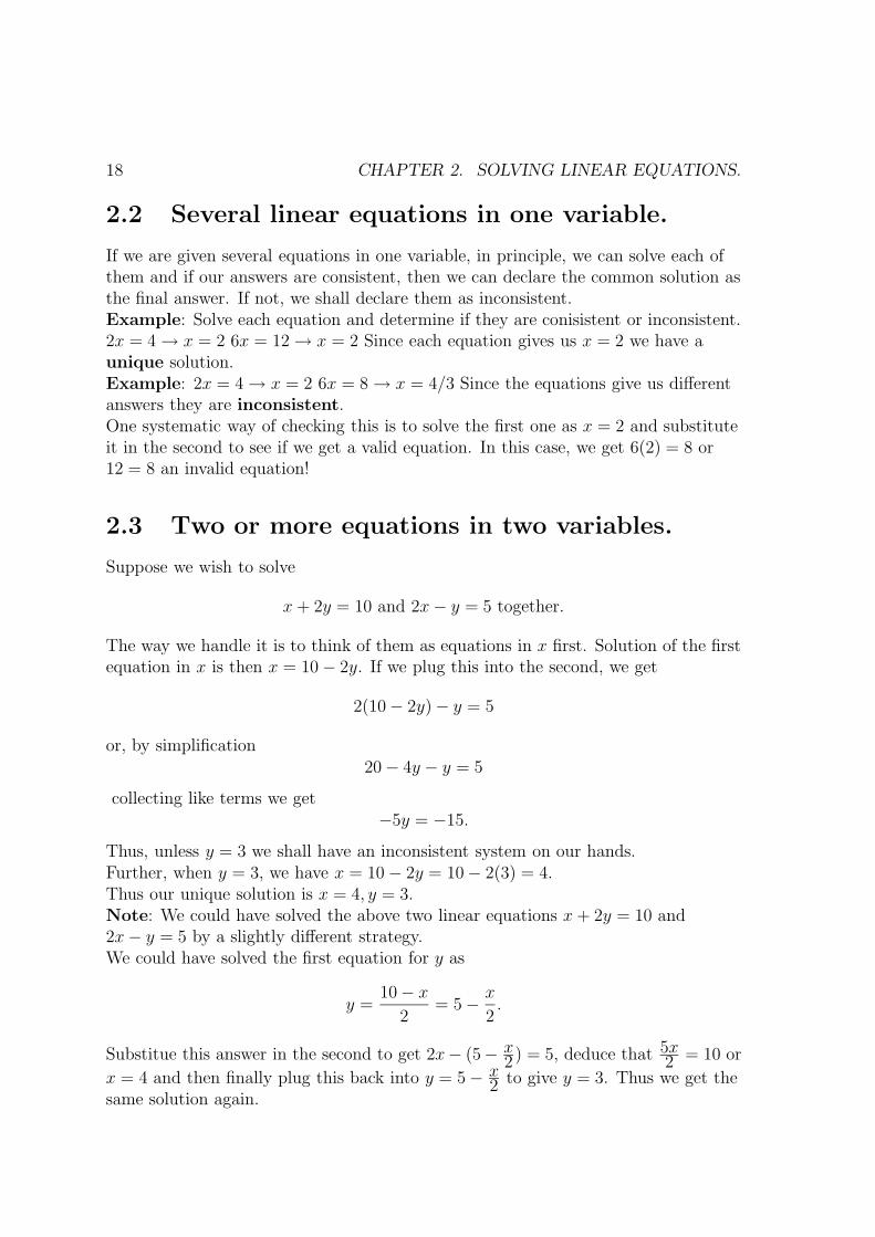
Thus, unless y = 3 we shall have an inconsistent system on our hands.Further, when y = 3, we have x = 10 − 2y = 10 − 2(3) = 4.Thus our unique solution is x = 4, y = 3.Note: We could have solved the above two linear equations x + 2y = 10 and2x − y = 5 by a slightly different strategy.We could have solved the first equation for y as
y =10 − x
2= 5 − x
2.
Substitue this answer in the second to get 2x− (5− x2 ) = 5, deduce that 5x
2 = 10 or
x = 4 and then finally plug this back into y = 5 − x2 to give y = 3. Thus we get the
same solution again.

2.4. SEVERAL EQUATIONS IN SEVERAL VARIABLES. 19
The choice the first variable is up to you, but sometimes it may be easier to solvefor one particular variable. With practice, you will be able to identify more easilywhich variable should be solved for first.Example:Solve x + 2y = 10, 2x − y = 5 and 3x + 4y = 10 together.We already know the unique solution of the first two; namely x = 4, y = 3. So, allwe need to do is plug it in the third to get 3(4) + 4(3) = 10 or 24 = 10. Since this isnot true, we get inconsistent equations and declare that that there is no solution.Example: If we change our problem to:
Solve x + 2y = 10 , 2x − y = 5 and 3x − 4y = 0 together;
then we get consistent equations with the known solution x = 4, y = 3.
2.4 Several equations in several variables.
Here is an example of solving three equations in x, y, z.
Solve: Eq1: x + 2y + z = 4 , Eq2: 2x − y = 3 , Eq3: y + z = 7.
We shall follow the above idea of solving one variable at a time.We solve Eq1 for x to get
Solution1. x = 4 − 2y − z
Substitution into Eq2, Eq3 gives two new equations in y, z:
2(4 − 2y − z) − y = 3 or y(−4 − 1) − 2z = 3 − 8 or 5y + 2z = 5.
The third has no x anyway, so it stays y + z = 7.Now we solve
Eq2∗ : 5y + 2z = 5 , Eq3∗ : y + z = 7.
Our technique says to solve one of them for one of the variables. Note that it iseasier to solve the equation Eq3∗ for y or z, so we solve it for y to get
Solution2. y = 7 − z
Finally, Eq2∗ becomes 5(7 − z) + 2z = 5 or z(−5 + 2) = 5 − 35. Thusz = −30/(−3) = 10. So we have:
Solution3. z = 10
Notice our three solutions. The third pins z down. Then the second saysy = 7 − z = 7 − 10 = −3.

20 CHAPTER 2. SOLVING LINEAR EQUATIONS.
Finally, the first one gives x = 4 − 2y − z = 4 − 2(−3) − (10) = 0 giving the: 3
Final solution. x = 0 , y = −3 , z = 10
This gives the main idea of our solution process. We summarize it formally below,as an aid to understanding and memorization.
• Pick some equation and a variable, say x, appearing in it.
• Solve the chosen equation for x and save this as the first solution. Substitutethe first solution in all the other equations.
These other equations are now free of x and represent a system with fewervariables.
• Continue to solve the smaller system by choosing a new variable etc. asdescribed above.
• When the smaller system gets solved, plug its solution into the original valueof x to finish the solution process.
2.5 Solving linear equations efficiently.
• Example 1. The process of solving for a variable and substituting in theother can sometimes be done more efficiently by manipulating the wholeequations. Here is an example.
Solve E1: 2x + 5y = 3 , E2: 4x + 9y = 5.
We note that solving for x and plugging it into the other equation is designedto get rid of x from the other equation. So, if we can get rid of x from one ofthe equation with less work, we should be happy.
The permissible operation (which still leads to the same final answers) is tochange one equation by adding a suitable multiple of one (or more) otherequation(s) to it.
By inspection, we see that E2-2E1 will get rid of x. So, we replace E2 byE2-2E1. We calculate this efficiently by collecting the coefficients as we go:
x(4 − 2(2)) + y(9 − 2(5)) = 5 − 2(3) or, after simplification − y = −1.
3The three solutions which give solutions for each of x, y, z in terms of later variables can beconsidered an almost final answer. Indeed, in a higher course on linear algebra, this is exactly whatdone! Given a set of equations, we order them somehow and try to get a sequence of solution givingeach variable in terms of the later ones. The resulting set of solution equations is often called therow echelon form.
2.5. SOLVING LINEAR EQUATIONS EFFICIENTLY. 21
So y = 1. The value of x is then easily determined by plugging this into eitherequation:
2x + 5(1) = 3 so x = (1/2)(3 − 5) = −1.
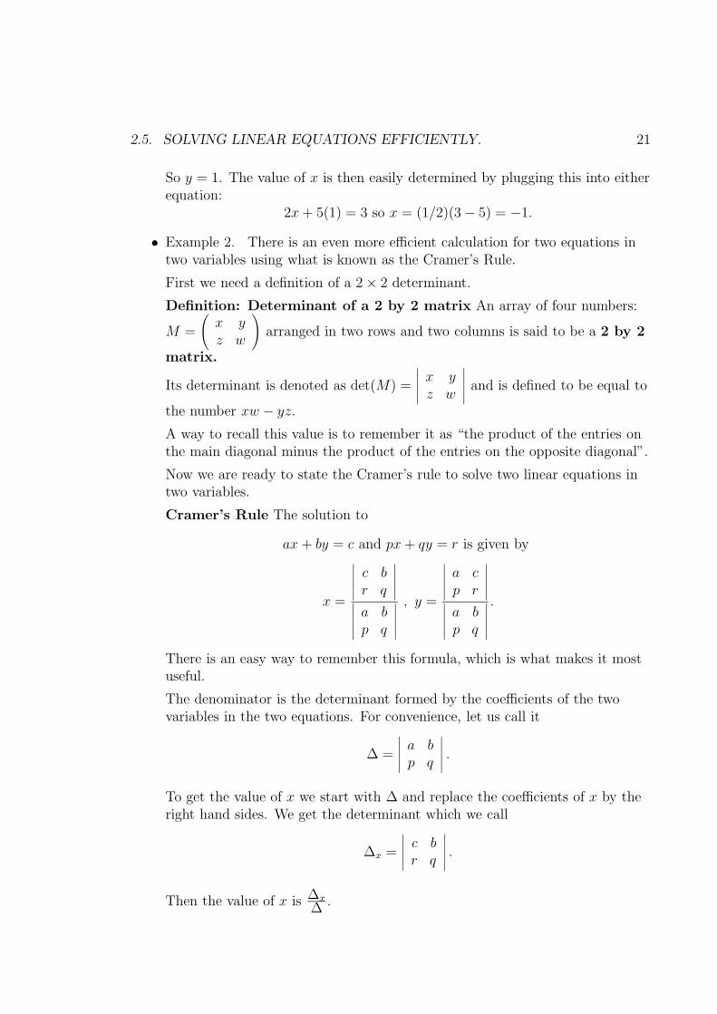
• Example 2. There is an even more efficient calculation for two equations intwo variables using what is known as the Cramer’s Rule.
First we need a definition of a 2 × 2 determinant.
Definition: Determinant of a 2 by 2 matrix An array of four numbers:
M =
(
x yz w
)
arranged in two rows and two columns is said to be a 2 by 2
matrix.
Its determinant is denoted as det(M) =
∣
∣
∣
∣
∣
x yz w
∣
∣
∣
∣
∣
and is defined to be equal to
the number xw − yz.
A way to recall this value is to remember it as “the product of the entries onthe main diagonal minus the product of the entries on the opposite diagonal”.
Now we are ready to state the Cramer’s rule to solve two linear equations intwo variables.
Cramer’s Rule The solution to
ax + by = c and px + qy = r is given by
x =
∣
∣
∣
∣
∣
c br q
∣
∣
∣
∣
∣
∣
∣
∣
∣
∣
a bp q
∣
∣
∣
∣
∣
, y =
∣
∣
∣
∣
∣
a cp r
∣
∣
∣
∣
∣
∣
∣
∣
∣
∣
a bp q
∣
∣
∣
∣
∣
.
There is an easy way to remember this formula, which is what makes it mostuseful.
The denominator is the determinant formed by the coefficients of the twovariables in the two equations. For convenience, let us call it
∆ =
∣
∣
∣
∣
∣
a bp q
∣
∣
∣
∣
∣
.
To get the value of x we start with ∆ and replace the coefficients of x by theright hand sides. We get the determinant which we call
∆x =
∣
∣
∣
∣
∣
c br q
∣
∣
∣
∣
∣
.
Then the value of x is ∆x∆ .

22 CHAPTER 2. SOLVING LINEAR EQUATIONS.
To get the y-value, we do the same with the y coefficients. Namely, we get
∆y =
∣
∣
∣
∣
∣
a cp r
∣
∣
∣
∣
∣
after replacing the coefficients of y by the right hand side.
Then the value of y is∆y
∆ .
To illustrate, let us solve the above example again.
Here the denominator is
∆ =
∣
∣
∣
∣
∣
2 54 9
∣
∣
∣
∣
∣
= (2)(9) − (4)(5) = −2.
The numerator for x is
∆x =
∣
∣
∣
∣
∣
3 55 9
∣
∣
∣
∣
∣
= (3)(9) − (5)(5) = 2.
The numerator for y is
∆y =
∣
∣
∣
∣
∣
2 34 5
∣
∣
∣
∣
∣
= (2)(5) − (4)(3) = −2.
So x = 2/(−2) = −1 and y = (−2)/(−2) = 1.
Exceptions to Cramer’s Rule. Our answers x = ∆x∆ and y =
∆y
∆ areclearly the final answers as long as ∆ 6= 0.
Thus we have a special case if and only if ∆ = aq − pb = 0. 4
Further, if one of the numerators is non zero, then there is no solution, while ifboth are zero, then we have infinitely many solutions.
The reader can easily verify these.
We shall illustrate this by some examples.
• Example 3.
Solve the system of equations:
2x + y = 5 , 4x + 2y = k
for various values of the parameter k.
4Thus ∆ lets us “determine” the nature of the solution. This is the reason for the term “deter-minant”.

2.5. SOLVING LINEAR EQUATIONS EFFICIENTLY. 23
If we apply the Cramer’s Rule, then we get
x =∆x
∆=
∣
∣
∣
∣
∣
5 1k 2
∣
∣
∣
∣
∣
∣
∣
∣
∣
∣
2 14 2
∣
∣
∣
∣
∣
=10 − k
0.
Similarly, we get 5
y =∆y
∆=
∣
∣
∣
∣
∣
2 54 k
∣
∣
∣
∣
∣
∣
∣
∣
∣
∣
2 14 2
∣
∣
∣
∣
∣
=2k − 20
0.
We see that when k 6= 10 then this leads to illegal values for x and y, while ifk = 10 then we are left with x = 0
0and y = 0
0.
We should not declare an answer right away, but try to analyze the situationfurther. A little thought shows that for k = 10 the second equation4x + 2y = 20 is simply twice the first equation 2x + y = 5 and so it can beforgotten as long as we use the first equation! Thus the solution set consists ofall values of x, y which satisfy 2x+y = 5. It is easy to describe these by saying:
Take any value, say t for y and then take x = 5−t2
. Some of the concreteanswers are x = 5
2, y = 0 using t = 0, or x = 2, y = 1 using t = 1, or
x = 3, y = −1 using t = −1 and so on. Indeed it is customary to declare: 6
x =5 − t
2, y = t where t is arbitrary.
Many linear equations in many variables.
There is a similar theory of solving many equations in many variables usinghigher order determinants. The interested reader may look up books ondeterminants or linear algebra.
• Example 4. Here, we shall only illustrate how the Cramer’s Rule mechanismworks beautifully for more variables, but we shall refrain from including thedetails of calculations. The reader is encouraged to search for the details.
5Technically, what we wrote is illegal! A true algebraist would insist on writing the equations as
(∆)x = ∆x or (0)x = 10 − k
and(∆)y = ∆y or (0)y = 2k − 20
6We shall see such answers when we study the parametric forms of equations of lines later.

24 CHAPTER 2. SOLVING LINEAR EQUATIONS.
Solve the three equations in three variables:
x + y + z = 6 , x − 2y + z = 0 and 2x − y − z = −3.
As befor, we make a determinant of the coefficients
∆ =
∣
∣
∣
∣
∣
∣
∣
1 1 11 −2 12 −1 −1
∣
∣
∣
∣
∣
∣
∣
.
As before, we get ∆x by replacing the x coefficients by the right hand sides:
∆ =
∣
∣
∣
∣
∣
∣
∣
6 1 10 −2 1
−3 −1 −1
∣
∣
∣
∣
∣
∣
∣
.
Once you get the right definition for a 3 by 3 determinant, it is easy tocalculate ∆ = −3 = ∆x, so x = −3
−3= 1.
Also, we get
∆y =
∣
∣
∣
∣
∣
∣
∣
1 6 11 0 12 −3 −1
∣
∣
∣
∣
∣
∣
∣
= −6.
Finally, we have
∆z =
∣
∣
∣
∣
∣
∣
∣
1 1 61 −2 02 −1 −3
∣
∣
∣
∣
∣
∣
∣
= −9.
This gives us y = −6−3
= 2 and z = −9−3
= 3. The reader can at least verify theanswers directly by known methods.

2.5. SOLVING LINEAR EQUATIONS EFFICIENTLY. 25

26 CHAPTER 2. SOLVING LINEAR EQUATIONS.

Chapter 3
The division algorithm andapplications
We have discussed addition, subtraction and multiplications of polynomials earlier.As indicated, we have a problem if we wish to divide one polynomial by another,since the answer may not be a polynomial again. Let us take an example ofu(x) = x3 + x, v(x) = x2 + x + 1. It is easy to see that the ratio u(x)
v(x)is not a
polynomial. To understand this, suppose it is equal to some polynomial w(x) andwrite the equation:
u(x)
v(x)= w(x) or u(x) = w(x)v(x).
We write this equation out and compare both sides.
x3 + x = (w(x))(x2 + x + 1).
By comparing the degrees of both sides, it follows that w(x) must have degree 1 inx. 1
Let us write w(x) = ax + b. Then we get
x3 + x = (ax + b)(x2 + x + 1) = ax3 + (a + b)x2 + (a + b)x + b.
Comparing coefficients of x on both sides, we see that we have:
a = 1 , a + b = 0 , (a + b) = 1 , b = 0.
Obviously these equations have no chance of a common solution, they areinconsistent! This proves that w(x) is not a polynomial!But perhaps we are being too greedy. What if we only try to solve the first two ofthe equations?
1Note that degx(u(x)) = deg
x(w(x)) + deg
x(v(x)) or 3 = deg
x(w(x)) + 2. Hence the conclusion.
27

28 CHAPTER 3. THE DIVISION ALGORITHM AND APPLICATIONS
Thus we solve a = 1 and a + b = 0 to get a = 1, b = −1. Then we see that usinga = 1, b = −1:
u(x) = x3 + x = (x − 1)(x2 + x + 1) + x + 1.
Let us name x − 1 as q(x) and x + 1 as r(x). Then we get:
u(x) = v(x)q(x) + r(x).
where r(x) has degree 1 which is smaller than the degree of v(x) which is 2.Thus, when we try to divide u(x) by v(x), then we get the best possible division asq(x) = x − 1 and a remainder x + 1.We now formalize this idea.Definition: Division Algorithm. Suppose that u(x) = axn + · · · andv(x) = bxm + · · · are polynomials of degrees n, m respectively and that v(x) is notthe zero polynomial. Then there are unique polynomials q(x) and r(x) whichsatisfy the following conditions:
1. u(x) = q(x)v(x) + r(x).
2. Moreover, either r(x) = 0 or
3. degx(r(x)) < degx(v(x)).
4. When the above conditions are satisfied, we declare that q(x) is the divisionand r(x) is the remainder when we divide u(x) by v(x).
5. The division q(x) and the remainder r(x) always exist and are uniquelydetermined 2 by u(x) and v(x).
First, we explain to find q(x) and r(x) systematically.Let us redo the problem with u(x) = x3 + x and v(x) = x2 + x + 1 again. Since uhas degree 3 and v has degree 2, we know that q must have degree 3 − 2 = 1.What we want is to arrange u − qv to have a degree as small as possible; this meansa degree of less than 2 or it may become zero!Start by guessing q = ax. Calculate
u − (ax)v = x3 + x − (ax)(x2 + x + 1) = (1 − a)x3 + (−a)x2 + (1 − a)x.
This means a = 1 and then we get
u − (x)v = (−1)x2.
2Hint for the proof: Suppose that u− q1v = r1 and u− q2v = r2 where r1, r2 are either 0 or havedegree less than m.
Subtract the second equation from the first and consider the two sides (q2 − q1)v and (r1 − r2).If both are 0, then you have the proof that q2 = q1 and r2 = r1. If one of them is zero, then the
other must be zero too, giving the proof.Finally, if both are non zero, then the left hand side has degree bigger than or equal to m while
the right hand side has degree less than m, a clear contradiction!

29
Our right hand side has degree 2 which is still not small enough! So we need toimprove our q. Add a next term to the current q = x and make it q = x + b.Recalculate: 3
u − (x + b)v = u − xv − bv= (−1)x2 − b(x2 + x + 1)= (−1 − b)x2 + (−b)x + (−b)
Thus, if we make −1 − b = 0 by taking b = −1, we get q(x) = x − 1 and
u(x) − q(x)v(x) = (−(−1))x + (−(−1)) = x + 1 = r(x).
Let us summarize this process:
1. Suppse u(x), v(x) have degrees n, m respectively where n ≥ m. (Note that weare naturally assuming that these are non zero polynomials.)
2. Start with a guess q(x) = ax(n−m) and choose a such that u − qv has degreeless than n.
3. The value of a will come out to be the leading coefficient of u divided by theleading coefficient of v. This formula is useful, but often it is easier to find aby inspection.
4. If the degree of u − qv is less than m or if it is zero, then stop and call it thefinal r.
5. If not, add a next term to q to make the degree of u − qv even smaller.
6. Continue until u − qv becomes 0 or its degree drops below m. What we aredescribing is the process of long division that you learnt in high school. Weare going to learn more efficient methods for doing it below.
There are two lucky situations where we need no more work! Let us record thesefor completeness.
1. In case u is the zero polynomial, we take q(x) = 0 and r(x) = 0. Check thatthis has the necessary properties!
2. In case u has degree smaller than that of v (i.e. n < m), we take q(x) = 0 andget r(x) = u(x). Check that this is a valid answer as well.
3. One important principle is to “let the definition be with you!!” If yousomehow see an answer for q and r which satisfies the conditions, then don’twaste time in the long division.
We now begin with an extension of the division algorithm.
3Note that we use the already done calculation of u−xv and don’t waste time redoing the steps.We only figure out the contribution of the new terms.
30 CHAPTER 3. THE DIVISION ALGORITHM AND APPLICATIONS
3.1 Repeated Division.
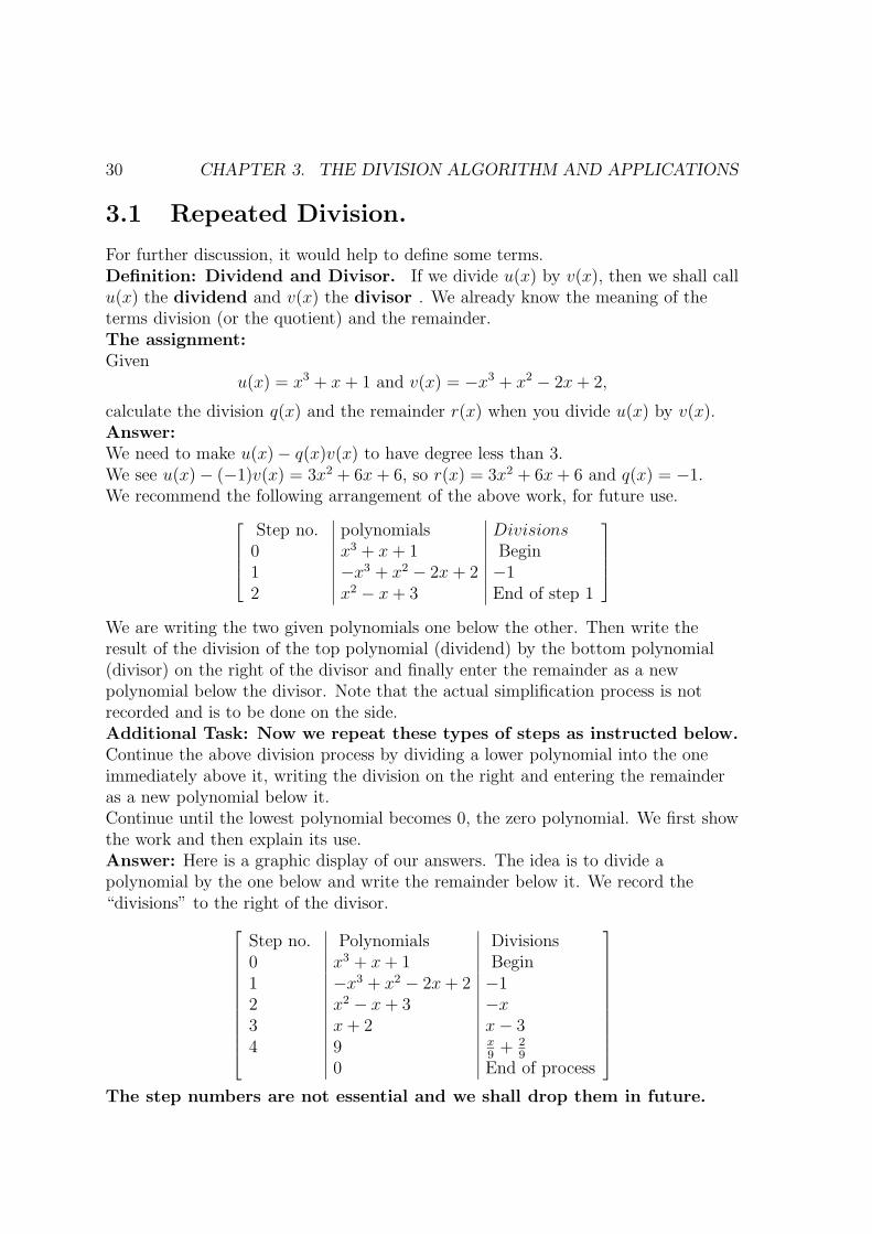
For further discussion, it would help to define some terms.Definition: Dividend and Divisor. If we divide u(x) by v(x), then we shall callu(x) the dividend and v(x) the divisor . We already know the meaning of theterms division (or the quotient) and the remainder.The assignment:Given
u(x) = x3 + x + 1 and v(x) = −x3 + x2 − 2x + 2,
calculate the division q(x) and the remainder r(x) when you divide u(x) by v(x).Answer:We need to make u(x) − q(x)v(x) to have degree less than 3.We see u(x) − (−1)v(x) = 3x2 + 6x + 6, so r(x) = 3x2 + 6x + 6 and q(x) = −1.We recommend the following arrangement of the above work, for future use.
Step no. polynomials Divisions0 x3 + x + 1 Begin1 −x3 + x2 − 2x + 2 −12 x2 − x + 3 End of step 1
We are writing the two given polynomials one below the other. Then write theresult of the division of the top polynomial (dividend) by the bottom polynomial(divisor) on the right of the divisor and finally enter the remainder as a newpolynomial below the divisor. Note that the actual simplification process is notrecorded and is to be done on the side.Additional Task: Now we repeat these types of steps as instructed below.Continue the above division process by dividing a lower polynomial into the oneimmediately above it, writing the division on the right and entering the remainderas a new polynomial below it.Continue until the lowest polynomial becomes 0, the zero polynomial. We first showthe work and then explain its use.Answer: Here is a graphic display of our answers. The idea is to divide apolynomial by the one below and write the remainder below it. We record the“divisions” to the right of the divisor.
Step no. Polynomials Divisions0 x3 + x + 1 Begin1 −x3 + x2 − 2x + 2 −12 x2 − x + 3 −x3 x + 2 x − 34 9 x
9+ 2
9
0 End of process
The step numbers are not essential and we shall drop them in future.
3.2. THE GCD AND LCM OF TWO POLYNOMIALS: MEANING AND CALCULATIONS.31
We are calculating these by the long division.The steps carried out above are for a purpose. These steps are used to find theGCD or the greatest common divisor (factor) of the original polynomials u(x), v(x).The reader is invited to deduce that our polynomials u(x), v(x) do not have acommon ( non constant) factor by the following steps:The equation u(x) − q(x)v(x) = r(x) says that any common factor of u(x), v(x)must be a factor of r(x). Thus a common factor of the top two polynomials in ourtable above must also divide the polynomial just below them (or the remainder).Repeating this idea, we see that the common factor must divide the last polynomialabove the zero polynomial.
3.2 The GCD and LCM of two polynomials:
meaning and calculations.
Indeed, this last polynomial (or any constant multiple of it) can be defined as theGCD.To make the idea of GCD precise, most algebraists would choose a multiple ofthe last polynomial which makes the highest degree corfficient equal to 1.To make this idea clear, we start with:Definition: Monic polynomial A nonzero polynomial in one variable is said tobe monic if its leading coefficient is 1. Note that the only monic polynomial ofdegree 0 is 1.Definition: GCD of two polynomials The GCD of two polynomials u(x), v(x)is defined to be a monic polynomial d(x) which has the property that d(x) dividesu(x) as well as v(x) and is the largest degree monic polynomial with this property.We shall use the notation:
d(x) = GCD(u(x), v(x)).
An alert reader will note that the definition gets in trouble if both polynomials arezero. Some people make a definition which produces the zero polynomial as theanswer, but we have to let go of the monicness condition. This case is usuallyexcluded!Definition: LCM of two polynomials The LCM (least common multiple) oftwo polynomials u(x), v(x) is defined as the smallest degree monic polynomial L(x)such that each of u(x) and v(x) divides L(x).As in case of GCD, we shall use the notation:
L(x) = LCM(u(x), v(x)).
If either of u(x) or v(x) is zero, then the only choice for L(x) is the zero polynomialand the degree condition as well as the monicness gets in trouble! As in the case ofGCD, we either agree that the zero polynomial is the answer or exclude such a case!

32 CHAPTER 3. THE DIVISION ALGORITHM AND APPLICATIONS
Calculation of LCM.Actually, it is easy to find LCM of two non zero polynomials u(x), v(x) by a simplecalculation. The simple formula is:
LCM(u(x), v(x)) = cu(x)v(x)
GCD(u(x), v(x)).
Here c is a constant which is chosen to make the LCM monic.There are occasional shortcuts to the calculation and these will be presented inspecial cases.The most important property of GCD. It is possible to show that the GCD oftwo polynomials u(x), v(x) is also the smallest degree monic polynomial whichcan be expressed as a combination a(x)v(x) − b(x)u(x).Below, we present the technique to find such a combination. The proof is left for theinquisitive reader to finish.For our polynomials above, the GCD will be the monic multiple of 9 and so theGCD of the given u(x), v(x) is said to be 1. 4
You may have seen a definition of the GCD of polynomials which tells you tofactorize both the polynomials and then take the largest common factor. This iscorrect, but requires the ability to factor the given polynomials, which is a verydifficult task in general. Our GCD algorithm is very general and useful in findingcommon factors without finding the factorization of the original polynomials.Our algorithm can also be adopted for finding the GCD of two given integers.Indeed that was the original formulation and application. We shall explain it below.
3.3 Aryabhata algorithm: Efficient Euclidean
algorithm.
Aryabhata algorithm gives us a way to solve the following problem. 5
Suppose that we are given two polynomial u(x), v(x) and wish to express a thirdpolynomial h(x) as their combination
h(x) = a(x)v(x) − b(x)u(x).
First let us study a very simple example. If we let u(x) = x and v(x) = x2 + x thenwe cannot write
1 = a(x)v(x) − b(x)u(x) = a(x)(x2 + x) − b(x)x.
4If you are confused about how 9 becomes 1, remember that the only monic polynomial of degree0 is 1.
5Indeed, this algorithm is usually known as the Euclidean algorithm. Our version is a moreconvenient arrangement of the algorithm given by an Indian Astronomer/Mathematician in the fifthcentury A.D., some 800 years after Euclid. It was, however, traditionally given in a much morecomplicated form by commentators. The original text is only one and a half verses long!

3.3. ARYABHATA ALGORITHM: EFFICIENT EUCLIDEAN ALGORITHM. 33
The simple reason is that if we set x = 0 the right hand side becomes 0 while theleft hand sides stays 1, so the two sides cannot be equal! 6
Thus, there is a condition on h(x). What is it?Let d(x) be the GCD of u(x), v(x), so using our notation, we shall write
d(x) = GCD(u(x), v(x)).
It is clear that d(x) divides the right hand side of the above equation for h(x) andhence must divide h(x).
Thus, the necessary condition is that the GCD of the two polynomials divides h(x).
Conversely, if d(x) divides h(x), then will soon show how to write h(x) as acombination of u(x) and v(x) as desired.
Illustration of the method.We shall show how to write h(x) = 1 as a combination b(x)v(x) − a(x)u(x) whereu(x) = x3 + x + 1 and v(x) = −x3 + x2 − 2x + 2. We already know that their GCDis 1, so our condition is valid.
The general method is similar and easily deduced from our description.
1. Start with the display of the division algorithm. By assumption, h(x) is theproduct of some w(x) and the last polynomial in our table just above the 0.For our example we get:
h(x) = 1 =1
9(9) − 0(0).
We begin a new column of answers next to the polynomials’ column by writngw(x) = 1
9at the bottom and 0 above it.
Thus we have the beginning of the answers’ column:
Answers Polynomials Divisionsx3 + x + 1 Begin−x3 + x2 − 2x + 2 −1x2 − x + 3 −xx + 2 x − 3
0 9 x9
+ 29
19
0 End of process
6This is a very efficient way of testing equality of two polynomials without the tedious task ofevaluating and comparing all their coefficients. Just substitute lots of values on both sides and seeif they give the same answer. If they ever fail to give the same answer, then they are unequal.
How many values do we need to check before we can declare them equal? It is possible to arguethat one more than their maximum degree is the magic number of values. This is left as a challengingexercise!
34 CHAPTER 3. THE DIVISION ALGORITHM AND APPLICATIONS
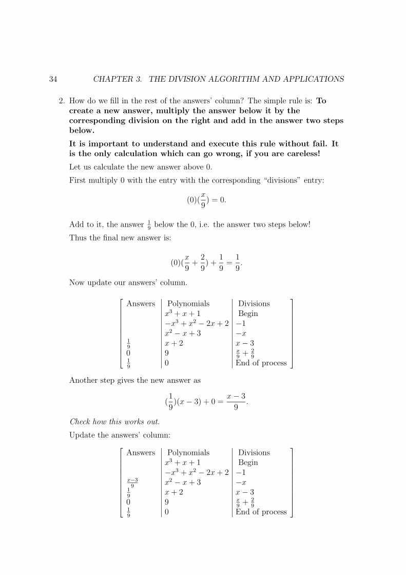
2. How do we fill in the rest of the answers’ column? The simple rule is: Tocreate a new answer, multiply the answer below it by thecorresponding division on the right and add in the answer two stepsbelow.
It is important to understand and execute this rule without fail. Itis the only calculation which can go wrong, if you are careless!
Let us calculate the new answer above 0.
First multiply 0 with the entry with the corresponding “divisions” entry:
(0)(x
9) = 0.
Add to it, the answer 19
below the 0, i.e. the answer two steps below!
Thus the final new answer is:
(0)(x
9+
2
9) +
1
9=
1
9.
Now update our answers’ column.
Answers Polynomials Divisionsx3 + x + 1 Begin−x3 + x2 − 2x + 2 −1x2 − x + 3 −x
19
x + 2 x − 30 9 x
9+ 2
919
0 End of process
Another step gives the new answer as
(1
9)(x − 3) + 0 =
x − 3
9.
Check how this works out.
Update the answers’ column:
Answers Polynomials Divisionsx3 + x + 1 Begin−x3 + x2 − 2x + 2 −1
x−39
x2 − x + 3 −x19
x + 2 x − 30 9 x
9+ 2
919
0 End of process

3.3. ARYABHATA ALGORITHM: EFFICIENT EUCLIDEAN ALGORITHM. 35
We show the result of next two steps at once. 7
Answers Polynomials Divisionsx2−2x−4
9x3 + x + 1 Begin
−x2+3x+19
−x3 + x2 − 2x + 2 −1x−39
x2 − x + 3 −x19
x + 2 x − 30 9 x
9+ 2
919
0 End of process
3. Now comes the reward for our calculations. Let
a(x) =x2 − 2x − 4
9and b(x) =
−x2 + 3x + 1
9.
.
Recall that our original polynomials are u(x) = x3 + x + 1 andv(x) = −x3 + x2 − 2x + 2 and we wished to write h(x) = 1 as theircombination.
Then our answer is
a(x)v(x) − b(x)u(x) = ±1 = ±h(x).
It is easy to figure out whether the sign is + or − by checking some term. Inour example, if we compute the constant term of a(x)v(x) − b(x)u(x), we see(−4/9)(2) − (1/9)(1) = −1, so we get −h(x). The correct answer to theproblem is then: 8
h(x) = 1 = −(a(x)v(x) − b(x)u(x))= b(x)u(x) − a(x)v(x)
= −x2+3x+19
(u(x)) − x2−2x−49
(v(x))
Example 1: Determine a polynomial P (x) such that when divided by x2 − 1 itgives a remainder x and when divided by x3 − 2 it gives a remainder 1 − x.Answer: ¿From the given conditions we get:
7For the reader’s convenience, here is the explanation of the very top answer x2−2x−4
9 .
Answer below is −x2+3x+1
9 and its corresponding divisions’ entry is −1. The answer two stepsbelow is x−3
9 , so we calculate:
(−x2 + 3x + 1
9)(−1) +
x − 3
9=
x2 − 3x − 1 + x − 3
9=
x2 − 2x − 4
9.
8An alert reader should note the determinant popping up in our expression. It is the topmosttwo by two determinant. Rule of the sign. It is possible to make a rule for the sign and it is this:The sign is + if the columns have an odd number of terms and − if they have even number of terms.It is, however, more reliable to actually check the sign.

36 CHAPTER 3. THE DIVISION ALGORITHM AND APPLICATIONS
1.P (x) = a(x)(x2 − 1) + x
and
2.P (x) = b(x)(x3 − 2) + 1 − x.
A simple subtraction gives:
a(x)(x2 − 1) − b(x)(x3 − 2) = x − (1 − x) = 2x − 1.
Thus we wish to write h(x) = 2x − 1 as a combination of the polynomials
u(x) = x3 − 2 and v(x) = x2 − 1.
We apply the above Aryabhata-Euclid algorithm. The reader should check thesesteps:
Step no. Polynomials Divisions0 x3 − 2 Begin1 x2 − 1 x2 x − 2 x + 23 3 x−2
3
0 End of process
Thus, we see that the GCD of the two polynomial divides 3 and hence is 1.Now we do the algorithm to write our h(x) = 2x − 1 as a combination as explainedby the Aryabhata algorithm.This means, we begin by writing the desired 2x − 1 as a combination of the last twopolynomials 3 and 0 in the simplest possible manner. Namely
2x − 1 =2x − 1
3(3) − 0(0).
We write the coefficients 0 and 2x−13
as the last two answers and lift them in theanswers’ column as before. 9
9As earlier, we explain the top entry 2x3 + 3x2 − 13 . It is obtained by calculating:
multiply2x2 + 3x − 2
3with x and add
2x − 1
3.
Note the evaluation:
2x3 + 3x2 − 2x
3+
2x − 1
3=
2x3 + 3x2 − 2x + 2x − 1
3.

3.3. ARYABHATA ALGORITHM: EFFICIENT EUCLIDEAN ALGORITHM. 37
Answers Polynomials Divisions2x3+3x2−1
3x3 − 2 Begin
2x2+3x−23
x2 − 1 x2x−1
3x − 2 x + 2
0 3 x−23
2x−13
0 End of process
Check that by setting
a(x) =2x3 + 3x2 − 1
3and b(x) =
2x2 + 3x − 2
3
we actually get
a(x)v(x) − b(x)u(x) = 2x − 1 = h(x).
What is the desired polynomial P (x)?Recall that we had P (x) = a(x)(x2 − 1) + x so we get
P (x) =2x3 + 3x2 − 1
3(x2 − 1) + x =
3x4 − 4x2 + 2x5 − 2x3 + 1 + 3x
3.
The Chinese Remainder Theorem or Kuttaka Our work above is the basis ofwhat is known as the Kuttaka in ancient Indian Mathematics. It is commonlyknown as the Chinese Remainder Theorem in modern mathematics books.The idea is to find a polynomial f(x) which has desired remainders r(x), s(x)respectively when divided by two given polynomials u(x) and v(x).We work as before, writing two equations:
f(x) = b(x)u(x) + r(x).
and
f(x) = a(x)v(x) + s(x)
After subtraction of the first equation from the second and a rearrangement, we getthe equation
a(x)v(x) − b(x)u(x) + s(x) − r(x) = 0 or r(x) − s(x) = a(x)v(x) − b(x)u(x).
You can see how the above algorithm can now be conveniently applied. We can alsoextend the theorem to several polynomials, but that would take us too far.Before turning to another topic, let us give an easier and older application of thisprocess for working with integers. Indeed, this is the more common application,rather than the polynomial version.

38 CHAPTER 3. THE DIVISION ALGORITHM AND APPLICATIONS
3.4 Division algorithm in integers.
Given two integers u, v where v is positive, we already know how to divide u by vand get a division and a remainder. This was taught as the long division of integersin schools.For instance, when we divide 23 by 5 we get the division 4 and remainder 3. Inequation form, we write this as
23 = (4)5 + 3.
For the readers who are very fond of their calculators, here is a simple recipe forfinding the division and the remainder.
• Have the calculator evaluate u/v. the division q is simply the integer part ofthe answer. Thus 23/5 = 4.6, so q = 4.
• Then calculate u − qv. This is the remainder r. Thus, we get 23 − (4)5 = 3,the remainder.
While useful, the above recipe can become unwieldy for large or complicatedintegers, so we urge the readers to not get dependent on it.Here is an example: Let u = 1 + 3 + 32 + 33 + · · ·+ 3100 and v = 3. Divide u by vand find the division q and the remainder r. The person with a calculator might beworking a long time and may get error messages from the calculator.A person who looks at the form can easily see that
u = 1 + 3(1 + 3 + · · ·+ 399) = r + 3q.
So we can happily declare: r = 1 and q = (1 + 3 + · · ·+ 399.You may not have seen much of the variations which we discuss next.Our choice u can be negative, say −23 and then we get:
−23 = (−5)5 + 2
so now the division is −5 and remainder is 2!The calculator person has to note that now u/v = −4.6 = −5 + 0.4. So the divisionis now taken as −5, since we want our remainder bigger than or equal to zero.Then u − qv = −23 − (−5)5 = −23 + 25 = 2 so r = 2.For better understanding, we record the definitions.Definition: Division Algorithm in Integers. Given two integers u, v withv 6= 0, there are unique integers q, r satisfying the following conditions:
1. u = qv + r and
2. 0 ≤ r < |v| where, as usual, |v| denotes the absolute value of v.

3.4. DIVISION ALGORITHM IN INTEGERS. 39
The integer q is the division and r is the remainder.
To continue our example above, let us now take v = −5 and note that|v| = | − 5| = 5, so we get the following:
If u = 23 then
23 = (−4)(−5) + 3 so q = −4 and r = 3.
The calculator work will give:
The ratio
u/v =23
−5= −4.6 = −4 − 0.6.
If we take q = −4, then we get u − qv = 23 − (−4)(−5) = 23 − 20 = 3 so r = 3.
Note that taking q = −5 makes a negative r in this case!
Definition: Divisibility of integers. We shall say that v divides u if u = kv forsome integer k. We write this in notation as v|u. Sometimes, this is also worded as“u is divisible by v”.
Thus, if v 6= 0 then we see that v|u exactly means that the remainder r when u isdivided by v becomes 0.
It is clear that the only integer divisible by 0 is 0.
Exercise. We leave it as an exercise to make a precise definition for divisibility ofpolynomials and provide suitable examples.
Definition: Divisibility of polynomials. Definition and examples to be suppliedby the reader!
Let us now apply the division algorithm to find the GCD of two integers. Forcompleteness, we record the definition:
Definition: GCD of integers. Given two integers u, v we say that an integer dis their GCD if the following conditions hold:
1. d divides both u, v.
2. If x divides both u and v then x divides d.
3. Either d = 0 or d > 0.
As before, for convenience, we define:
Definition: LCM of integers. Given two integers u, v we say that an integer Lis their LCM if the following conditions hold:
1. Each of u, v divides L.
2. If each of u, v divide x, then L divides x.
3. Either L = 0 or L > 0.

40 CHAPTER 3. THE DIVISION ALGORITHM AND APPLICATIONS
As before, we have a simple fact:Calculation of LCM.Actually, it is easy to find LCM of two non zero integers u, v by a simplecalculation. The simple formula is:
LCM(u, v) = cuv
GCD(u, v).
Here c is equal to 1 or −1 and is chosen such that the LCM comes out positive.Remarks. First note that the definitions of GCD and LCM can be easily extendedto include several integers rather than just two u, v. The reader is encouraged to dothis. Next note that d = 0 exactly when u = v = 0.Important Fact. If we had to check these definitions every time, then the GCDwould be a complicated concept. However, we show how to effectively find the GCDusing the Aryabhata-Euclid algorithm. Moreover, we get it in the form of acombination of u and v.We show this by the following:Example 2: Find the GCD of 18 and 14 and write it as a combination of 18 and14.Moreover, find an integer n such that n gives remainder 1 when divided by 18 and aremainder of 5 when divided by 14.Answer: We apply the same algorithm as we did in polynomials. The reader isencouraged to fill in the justification.
1. Finding the GCD. Just imitate the Aryabhata algorithm!
Step no. Integers Divisions0 18 Begin1 14 12 4 33 2 2
0 End of process
The GCD is the number 2 above the 0.
2. Writing the GCD as a combination of the given integers. Again, imitate thesame steps as in the polynomial case.
Answers Integers Divisions4 18 Begin3 14 11 4 30 2 21 0 End of process
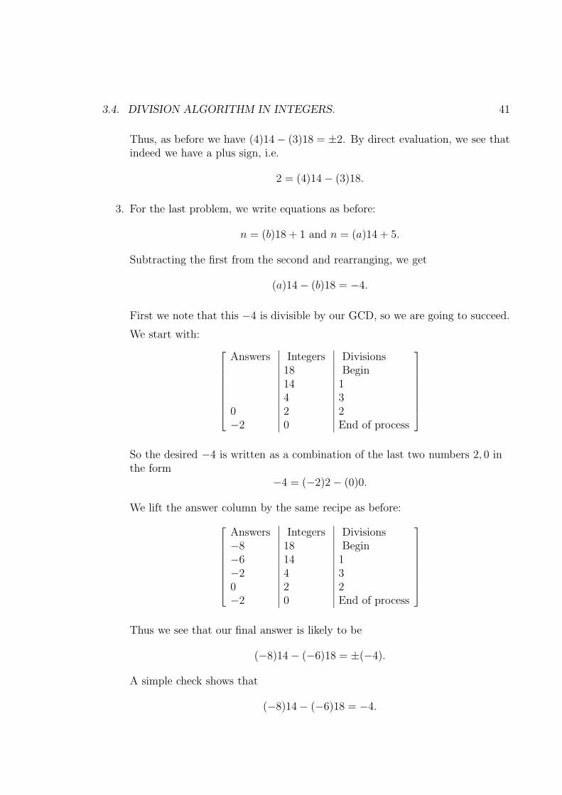
3.4. DIVISION ALGORITHM IN INTEGERS. 41
Thus, as before we have (4)14 − (3)18 = ±2. By direct evaluation, we see thatindeed we have a plus sign, i.e.
2 = (4)14 − (3)18.
3. For the last problem, we write equations as before:
n = (b)18 + 1 and n = (a)14 + 5.
Subtracting the first from the second and rearranging, we get
(a)14 − (b)18 = −4.
First we note that this −4 is divisible by our GCD, so we are going to succeed.
We start with:
Answers Integers Divisions18 Begin14 14 3
0 2 2−2 0 End of process
So the desired −4 is written as a combination of the last two numbers 2, 0 inthe form
−4 = (−2)2 − (0)0.
We lift the answer column by the same recipe as before:
Answers Integers Divisions−8 18 Begin−6 14 1−2 4 30 2 2−2 0 End of process
Thus we see that our final answer is likely to be
(−8)14 − (−6)18 = ±(−4).
A simple check shows that
(−8)14 − (−6)18 = −4.
42 CHAPTER 3. THE DIVISION ALGORITHM AND APPLICATIONS
This gives us a = −8, b = −6 and hence
n = (b)18 + 1 = (−6)18 + 1 = −107.
We found an answer, but perhaps we want a positive answer. Is there one?
Indeed, there is! We can add any multiple of the LCM(14, 18) to our answerand its stays a valid answer.
Since the LCM is (14)(18)/2 = 126 we use it. (Note that we are using theLCM formula given above.)
So 126 − 107 = 19 is a possible answer as well! Indeed 19 does give theremainder 1 when divided by 18 and remainder 5 when divided by 14. So,here a trial and error method could have been more efficient! However, wecannot, however, count on trial and error!
Example 3: Let a be a constant. Find the division and remainder when (x − a)divides various powers of x, like x, x2, x3, x4, · · ·.Using these results deduce a formula to compute the remainder when a polynomialf(x) is divided by (x − a).Answer: The main point to note is this:If we can somehow guess answers q(x), r(x) such that
•u(x) − q(x)v(x) = r(x)
• and either r(x) = 0 or the degree of r(x) is less than that of v(x),
then we have found our division and remainder! No long division is actually needed.If we divide (x − a) by (x − a), we clearly have q(x) = 1, r(x) = 0.In view of the identity
x2 − a2 = (x − a)(x + a)
we get by rearrangement:
x2 − (x + a)(x − a) = a2
so, dividing x2 by x − a gives division (x + a) and remainder a2.To divide x3 by (x − a), we start with the above relation and multiply it by x, so:
x3 − x(x + a)(x − a) = a2x = a2(x − a) + a3
i.e. we getx3 − (x(x + a) + a2)(x − a) = a3.
This simplifies to:
x3 − (x2 + ax + a2)(x − a) = a3 giving q(x) = x2 + ax + a2 and r(x) = a3.

3.4. DIVISION ALGORITHM IN INTEGERS. 43
The reader is invited to repeat this idea and deduce
x4 − (x)(x2 + ax + a2)(x − a) − a3(x − a) = a4
or
x4−(x3 +ax2 +a2x+a3)(x−a) = a4 giving q(x) = x3 +ax2 +a2x+a3 and r(x) = a4.
It is not hard to imagine and prove the identity:
xn − (xn−1 + axn−2 + · · · + an−1)(x − a) = an for n = 1, 2, · · · .
Thus in general the remainder of xn is an. It is easy to see that the remainder of cxn
will be can for a constant c and generally for any polynomial f(x) the remainderwhen divided by (x − a) shall be f(a).10
We have thus proved the well knownRemainder theorem The linear expression (x − a) divides a polynomial f(x) ifand only if f(a) = 0.We have also proved, in view of our concrete steps:The geometric series formulaFor any positive integer n we have
1 + x + · · · + xn−1 =xn − 1
x − 1.
For proof, proceed as follows:
• Start with the known identity:
xn − (xn−1 + axn−2 + · · ·+ an−1)(x − a) = an.
• Set a = 1 and deduce:
xn − (xn−1 + xn−2 + · · · + 1)(x − 1) = 1
• Rewrite as:xn − 1 = (xn−1 + xn−2 + · · ·+ 1)(x − 1).
Divide by (x − 1) and finish!
10For proof, the reader may try this idea.Given a divisor v(x), a general remainder of a polynomial u(x) shall be defined as any polynomial
of the form u(x)− h(x)v(x) and a good remainder is one which is either 0 or of degree smaller thanthat of v(x). Thus the division algorithm simply asks us to find the unique good remainder! Notethat by definition, a constant times a good remainder is again a good remainder and so is a sum oftwo good remainders. It is easy to show that this finishes the proof.
44 CHAPTER 3. THE DIVISION ALGORITHM AND APPLICATIONS
Example 4: Let a be a constant. Find the division and the remainder when(x2 − a) divides various powers of x, x2, x3, x4, · · ·.Using these results, deduce a formula for the remainder when a polynomial f(x) isdivided by (x2 − a).Answer: As before we do some initial cases for understanding and experience: Wewish to divide various xn by x2 − a and find the division and remainder.
Case n = 0x0 = 1 = (0)(x2 − a) + 1 so q(x) = 0, r(x) = 1.
Case n = 1x1 = x = (0)(x2 − a) + x so q(x) = 0, r(x) = x.
Case n = 2x2 = x2 = (x2 − a) + a so q(x) = 1, r(x) = a.
Case n = 3x3 = x(x2 − a) + ax so q(x) = x, r(x) = ax.
Case n = 4
x4 = x2(x2 − a) + a(x2 − a) + a2 so q(x) = x2 + a, r(x) = a2.
Case n = 5
x5 = x(x2 + a)(x2 − a) + a2x so q(x) = x3 + ax, r(x) = a2x.
Case n = 6
x6 = x2(x3 + ax)(x2 − a) + a2(x2 − a) + a3 so q(x) = x4 + ax2 + a2, r(x) = a3.
This is enough experience!Look at the answers for even powers:
n = q(x) r(x)2 1 a4 x2 + a a2
6 x4 + ax2 + a2 a3
We now guess and prove the formula for x8. The guess isq(x) = x6 + ax4 + a2x2 + a3 and r(x) = a4.The proof is this:
x8 = x2(x6)= x2(x4 + ax2 + a2)(x2 − a) + x2(a3)= x2(x4 + ax2 + a2)(x2 − a) + (x2 − a)(a3) + a4
= (x6 + ax4 + a2x2 + a3)(x2 − a) + a4.

3.4. DIVISION ALGORITHM IN INTEGERS. 45
Here is a challenge to your imagination and hence a quick road the answer!Name the quantity x2 as y and note that then we are trying to divide it by (y − a).We already learned how to find the answers as polynomials in y. use them and theplug back y = x2 to get our current answers!But what do we do for an odd power? Suppose that we know the answer for an evenpower:
x2m = q(x)(x2 − a) + r(x).
We now know that r(x) = am.Then the answer for x2m+1 shall be given as:
x2m+1 = x(q(x)(x2 − a) + r(x)) = xq(x)(x2 − a) + amx.
Combining the above work, we see that we at least have the complete formula forthe remainders of xn. It is this: Write n = 2m + s where s = 0 or 1. (In otherwords, s is the remainder when we divide n by 2.)Then the remainder of xn is amxs!For a general polynomial, rather than writing a general formula, let us illustrate themethod.Say f(x) = x5 + 2x4 + x3 − x + 3. Find the remainder when it is divided by x2 − 2.The remainders of the five terms are as follows:
term Even or odd remainderx5 odd 22x = 4x2x4 even 2(22) = 8x3 odd 2x−x odd (−1)x = −x3 even 3
So finally the remainder of f(x) is
4x + 2x − x + 8 + 3 = 5x + 11.
Note that we have note kept track of q(x). If we need it, we can use the definitionand calculate by dividing f(x) − r(x) by x2 − 2.Enhanced remainder theorem!Here is an even simpler idea to calculate the remainder. Note that we ultimatelyhave f(x) = q(x)(x2 − a) + r(x). If we agree to replace every “x2” by a in f(x), thenwe notice that on the right hand side the part q(x)(x2 − a) will become zero. So,f(x) will eventually reduce to the remainder!Here is how this wonderful idea works for our problem solved above:
Current polynomial Explanationx5 + 2x4 + x3 − x + 3 Start2x3 + 4x2 + 2x − x + 3 x2 in each term is replaced by 24x + 8 + 2x − x + 3 two more reductions done5x + 11 collected terms

46 CHAPTER 3. THE DIVISION ALGORITHM AND APPLICATIONS
Naturally, this is much easier than the actual division.

3.4. DIVISION ALGORITHM IN INTEGERS. 47

48 CHAPTER 3. THE DIVISION ALGORITHM AND APPLICATIONS
Chapter 4
Introduction to analytic geometry.
While algebra is a powerful tool of calculations, it is not so helpful for visualizationand intuition for a beginning student. Also, many important motivations for algebraoriginally came from geometric ideas. Hence, we next introduce the algebraicversion of geometric concepts.
Here is a quick summary of our plan. We think of the geometric objects called lines,planes, three space, etc. These are made up of points. We associate numbers (singleor multiple) to each points so that we can express various geometric concepts andcalculations as algebraic concepts and calculations.
In geometry, we first study points in a line, then a plane and then a three (orhigher) dimensional space.
4.1 Coordinate systems.
To work with a line, we agree to choose a special point called the “origin” and ascale so that a certain other point is at a distance of 1 unit from the origin - to becalled a unit point. This sets up a system of coordinates (associated real numbers)to every point of the line and we can handle the points by using the algebraicoperations of real numbers.
To work with a plane, we agree to set up a special point called the origin and apair of perpendicular lines called the x and y axes.
On each of the axes, we agree to a scale so that every axis has a coordinate systemof its own. Then every point in the plane can be associated with a pair of realnumbers called coordinates and these are described in the following way:
Given any point P in the plane, draw a line from it parallel to the y axis and thecoordinate of the point where it hits the x axis is called the x coordinate of P .Similarly a line is drawn through P parallel to the x axis and its intersection withthe y axis is the y coordinate of P . If these coordinates are (a, b) respectively, thenwe simply write P (a, b) or say that P is the point (with coordinates) (a, b).
49
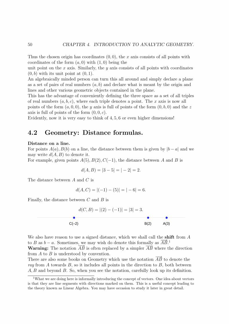
50 CHAPTER 4. INTRODUCTION TO ANALYTIC GEOMETRY.
Thus the chosen origin has coordinates (0, 0), the x axis consists of all points withcoordinates of the form (a, 0) with (1, 0) being theunit point on the x axis. Similarly, the y axis consists of all points with coordinates(0, b) with its unit point at (0, 1).An algebraically minded person can turn this all around and simply declare a planeas a set of pairs of real numbers (a, b) and declare what is meant by the origin andlines and other various geometric objects contained in the plane.This has the advantage of conveniently defining the three space as a set of all triplesof real numbers (a, b, c), where each triple denotes a point. The x axis is now allpoints of the form (a, 0, 0), the y axis is full of points of the form (0, b, 0) and the zaxis is full of points of the form (0, 0, c).Evidently, now it is very easy to think of 4, 5, 6 or even higher dimensions!
4.2 Geometry: Distance formulas.
Distance on a line.For points A(a), B(b) on a line, the distance between them is given by |b− a| and wemay write d(A, B) to denote it.For example, given points A(5), B(2), C(−1), the distance between A and B is
d(A, B) = |3 − 5| = | − 2| = 2.
The distance between A and C is
d(A, C) = |(−1) − (5)| = | − 6| = 6.
Finally, the distance between C and B is
d(C, B) = |(2) − (−1)| = |3| = 3.
C(–2) B(2) A(3)
We also have reason to use a signed distance, which we shall call the shift from Ato B as b − a. Sometimes, we may wish do denote this formally as
−→AB.1
Warning: The notation−→AB is often replaced by a simpler AB where the direction
from A to B is understood by convention.There are also some books on Geometry which use the notation
−→AB to denote the
ray from A towards B, so it includes all points in the direction to B, both betweenA, B and beyond B. So, when you see the notation, carefully look up its definition.
1What we are doing here is informally introducing the concept of vectors. One idea about vectorsis that they are line segments with directions marked on them. This is a useful concept leading tothe theory known as Linear Algebra. You may have occasion to study it later in great detail.
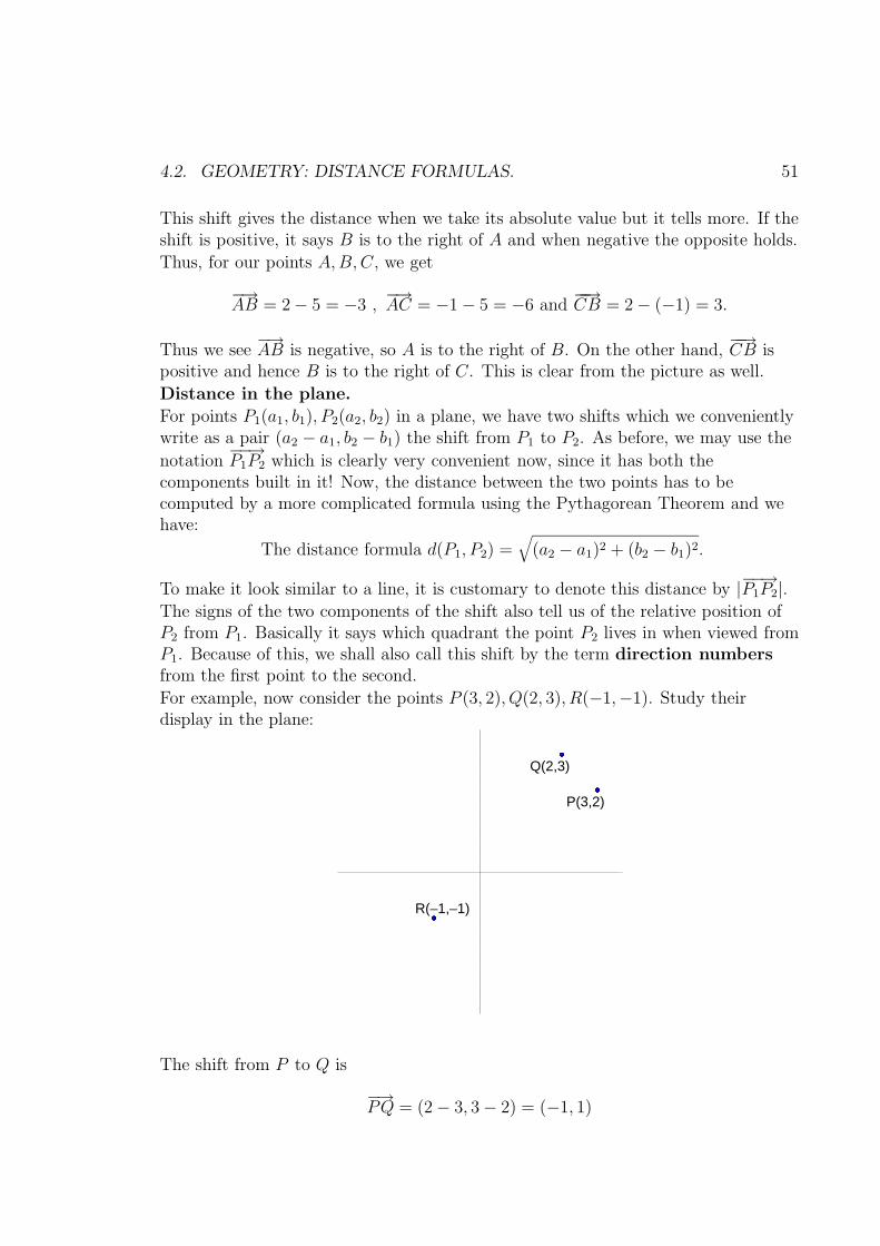
4.2. GEOMETRY: DISTANCE FORMULAS. 51
This shift gives the distance when we take its absolute value but it tells more. If theshift is positive, it says B is to the right of A and when negative the opposite holds.
Thus, for our points A, B, C, we get
−→AB = 2 − 5 = −3 ,
−→AC = −1 − 5 = −6 and
−−→CB = 2 − (−1) = 3.
Thus we see−→AB is negative, so A is to the right of B. On the other hand,
−−→CB is
positive and hence B is to the right of C. This is clear from the picture as well.
Distance in the plane.
For points P1(a1, b1), P2(a2, b2) in a plane, we have two shifts which we convenientlywrite as a pair (a2 − a1, b2 − b1) the shift from P1 to P2. As before, we may use the
notation−−→P1P2 which is clearly very convenient now, since it has both the
components built in it! Now, the distance between the two points has to becomputed by a more complicated formula using the Pythagorean Theorem and wehave:
The distance formula d(P1, P2) =√
(a2 − a1)2 + (b2 − b1)2.
To make it look similar to a line, it is customary to denote this distance by |−−→P1P2|.The signs of the two components of the shift also tell us of the relative position ofP2 from P1. Basically it says which quadrant the point P2 lives in when viewed fromP1. Because of this, we shall also call this shift by the term direction numbersfrom the first point to the second.
For example, now consider the points P (3, 2), Q(2, 3), R(−1,−1). Study theirdisplay in the plane:
R(–1,–1)
Q(2,3)
P(3,2)
The shift from P to Q is
−→PQ = (2 − 3, 3 − 2) = (−1, 1)

52 CHAPTER 4. INTRODUCTION TO ANALYTIC GEOMETRY.
and the distance from P to Q is
d(P, Q) =√
(−1)2 + (1)2 =√
2.
Notice that from the position P , the point Q does appear to be one unit to the leftand one unit up!Verify that for the points Q, R, we get
−→QR = (−1 − 2,−1 − 3) = (−3,−4) and
d(Q, R) =√
(−3)2 + (−4)2 =√
25 = 5.
Similarly for the points R, S, we get−→QR = (−1 − 3,−1 − 2) = (−4,−3) and hence
the distance d(R, S) = 5 also.We can similarly handle points in a three dimensional space and set up shifts anddistance formulas. The third and higher dimensions can be handled as needed.
4.3 Change of coordinates on a line.
In the case of the coordinates of a line, we had to choose an origin and then a scaleand indeed we inadvertently chose a direction as well by deciding where the unitpoint is.What happens if we choose a different origin and a different scale?Clearly the coordinates of a point will change. We would like to create an algebraicrecipe for the resulting change.We illustrate this by an example.Let us say that we have a coordinate system so that each point P (a) has anassigned coordinate. We would like to choose a new origin at the point Q(3) - thepoint with current coordinate 3. Let x be the value of the original coordinate of apoint and let x′ be its new coordinate. Then we claim that
x′ = x − 3
We shall say that under this coordinate change the point A(x) goes to the pointA′(x − 3).Thus the point Q(3) goes to the point Q′(3 − 3) = Q′(0). This is the new origin!Also, it is easy to see that the distance between any two points stays unchangedwhether we use the x or the x′coordinates. 2
A most general change of coordinates can be described by a substitution x′ = ax + bwhere a is non zero. Its effect can be analyzed as described below.
1. Case a > 0: The origin is shifted to the point with x-coordinate −b/a. Allshifts are multiplied by a and hence the direction is preserved. The distancesare also scaled (multiplied) by a.
2An alert reader should observe that the distance between two points P1(a1), P2(a2) is given by|a2 − a1|. So, in new coordinates it becomes |(a2 − 3) − (a1 − 3)| = |a2 − a1|, or is unchanged.
Indeed, the new coordinate also preserves all shifts.

4.4. CHANGE OF COORDINATES IN THE PLANE. 53
For example, let a = 3, b = −1. Consider the points P (2), Q(5). The newcoordinate of P shall be 3(2) − 1 = 5.
Similarly for the point Q we get 3(5) − 1 = 14.
The original shift−→PQ = 5 − 2 = 3. The new shift is 14 − 5 = 9 which is 3
times the old shift.
The distance 3 becomes 3(3) = 9.
2. Case a < 0: The origin is still shifted to the point with x-coordinate −b/a. Allshifts are multiplied by a < 0 and hence the direction is reversed. Thedistances are scaled (multiplied) by |a| = −a.
For example, let a = −2, b = −5.
For the same points P (2), Q(5), the new coordinates become (−2)2 − 5 = −9and (−2)5 − 5 = −15. Thus P (2) goes to P ′(−9) and Q(5) goes to Q′(−15).
Thus the new shift−−→P ′Q′ is −15 − (−9) = −6 which is indeed the old shift−→
PQ = 3 multiplied by a = −2. The distance changes from 3 to 6.
The reader should investigate what happens to the unit points or other specificgiven points.
4.4 Change of coordinates in the plane.
We can easily generalize the above formulas and get similar results. Thus we have:
1. Translation or Change of origin only. A transformation x′ = x − p , y′ = y − qchanges the origin to the point with original (x, y) coordinates (p, q). All shiftsand distances are preserved.
2. Change of origin with axes flips. A transformation x′ = ux − p, y′ = vy − qwhere u, v are ±1 changes the origin to the point with original (x, y)coordinates (up, vq).
All distances are preserved. However, shifts can change and we list theirproperties:
Value of u Value of v Effect1 −1 y axis is flipped. A reflection about the x axis.
−1 1 x axis is flipped. A reflection about the y axis.−1 −1 Both axes are flipped. A reflection about the origin.
Thus, the transformation consists of first a translation to make (up, uq) as thenew origin followed by the indicated flip(s).

54 CHAPTER 4. INTRODUCTION TO ANALYTIC GEOMETRY.
The proof simply consists of comparing effects on points. This is best done byplotting the original points and their images on the same graph paper.
As an illustration, let us see what a transformation x′ = −x − 5 , y′ = y − 4does. The point P (−5, 4) becomes (0, 0) or the new origin.
All points of the form (a, 4) get transformed to (−a − 5, 0) i.e. become thenew x′ axis. The point (−5 + 1, 4) = (−4, 4) which has a shift of (1, 0) from Pgoes to (−1, 0) showing that there is a flip of the x axis direction.
Similarly the points (−5, b) will map to the (0, b − 4) to become the new y ′
axis. There is no flip involved, since the point (−5, 5) with shift (0, 1) from Pgoes to (0, 1).
The general idea consists of three steps.
(a) First determine what becomes the new origin - say it is P (p, q).
(b) Then find the images of P1(p + 1, q) and P2(p, q + 1).
(c) Compare the original triangle PP1P2 with its image for any possible flips!
4.5 General change of coordinates:
We can indeed stretch these ideas to analyze a general change of coordinates. Wewill, however, leave the analysis for higher courses. Here we only state the mostimportant facts for information and as a challenge for the super smart ones.The most general coordinate change in the plane can be written as
x′ = a(x − p) + b(y − q) , y′ = c(x − p) + d(y − q).
where a, b, c, d are constants such that the determinant
∣
∣
∣
∣
∣
a bc d
∣
∣
∣
∣
∣
= ad − bc 6= 0.
It is easy to see that the origin is shifted to the point with original coordinates(p, q), but shifts and distances change in a complicated manner. If you wish tostudy geometric properties like distances and angles, you must investigate changeswhich preserve distances. These are the so called isometries (“iso” means same,“metry” is related to measure)!The changes of coordinates which preserve distances can be described nicely usingtrigonometry. We, however, choose to postpone these discussions to a higher course.We will give a brief sample of this in a later chapter.3
3Here are the details for the inquisitive.We know how to translate and so for this part, we assume that there is no translation involved.Distance preserving transformations can be achieved exactly when there is an angle θ and a
number u = ±1 such that
x′ = cos(θ)x + sin(θ)y , y′ = −u sin(θ)x + u cos(θ)y.

4.5. GENERAL CHANGE OF COORDINATES: 55
Examples of changes of coordinates:We illustrate the above discussion by various examples.
Example 1 Find a transformation on the line which changes the point A(3) to A′(5) andB(−1) to B′(1).
Use your answer to find out the new coordinate of the point C(3). Also, ifD(d) goes to D′(−5) what is d?
Answer:
• We assume that the transformation is x′ = px + q and try to find p, q.¿From the information about the point A, we see that
5 = p(3) + q = 3p + q.
The information about B says:
1 = p(−1) + q = −p + q.
We need to solve these two equations together. Of course, we can use anyof the techniques that we know, but here, it is easiest to subtract thesecond from the first to get:
4 = 3p + q − (−p + q) = 4p.
So p = 1. Plugging the value of p into the first equation, we see that:
5 = 3 + q so q = 2.
Thus the transformation is:
x′ = x + 2.
• To find the image of C(3), we set x = 3 and deduce that x′ = 3 + 2 = 5.So, C(3) becomes C ′(5).
• To find the point D, we set x′ = −5 and solve −5 = x + 2 to get x = −7.So d = −7.
The transformation can be described as a rotation by θ if u = 1 and this is followed by a flip of they′ axis if u = −1. The trigonometric functions cos(θ), sin(θ) have been studied from ancient timesand here is a quick definition when 0 < θ < 90. Make a triangle ABC where the angle at B is thedesired θ and the one at C is 90 degrees. Then
cos(θ) = |−−→BC |/|−−→BA| and sin(θ) = |−→CA|/|−−→BA|.
For other values of angles, these are defined by suitable adjustments. We will give a more generalmodern definition during the discussion of the circles.

56 CHAPTER 4. INTRODUCTION TO ANALYTIC GEOMETRY.
Example 2 Find a plane transformation using only translations and flips which sendsP (1, 1) to P ′(4, 1), Q(2, 3) to Q′(5, 1).
Determine the new image of the origin. Also determine the point which goesto the new origin.
What point R goes to R′(3, 3)?
Answer:
• Assume that the transformation is given by
x′ = ux − p, vy − q.
We have the equations for point P :
4 = u − p , 1 = v − q.
Similarly for the point Q, we get:
5 = 2u − p , 1 = 3v − q.
The reader can verify the solution:
u = 1, p = −3, v = −1, q = −2.
Thus the transformation is:
x′ = x + 3 , y′ = −y + 2.
• Clearly, the origin O(0, 0) goes to O′(3, 2).
• If x′ = 0 and y′ = 0 then clearly, x = −3 and y = 2, so the point S(−3, 2)becomes the new origin!
• If x′ = 3 and y′ = 3, then x = 0 and y = −1, so R(0,−1) is the desiredpoint.

4.5. GENERAL CHANGE OF COORDINATES: 57

58 CHAPTER 4. INTRODUCTION TO ANALYTIC GEOMETRY.
Chapter 5
Equations of lines in the plane.
Given a point P (a, b) in the plane, it is easy to see that the line joining it with theorigin consists of all points of the form (at, bt) as t varies over the real numbers. Wecan conveniently call such a point Q(t).Thus, if we write O for the origin, then we can describe our formula as
−→OQ = (at, bt) = t(a, b) = (t)(
−→OP ) for some real t .
More generally, a line joining a point P1(a1, b1) to P2(a2, b2) can then be described
as all points Q(x, y) such that−−→P1Q = (t)(
−−→P1P2), i.e.
(x − a1, y − b1) = t(a2 − a1, b2 − b1) and this gives us the:
Parametric two point form: x = a1 + t(a2 − a1) , y = b1 + t(b2 − b1).
The shift−−→P1P2 can be conveniently denoted as P2 − P1, where we think of the points
as pairs of coordinates and perform natural term by term operations on them. Now,our formula can be conveniently written as:
Compact parametric two point form: Q(x, y) = P1 + t(P2 − P1).
Note that this formula can also be rewritten as: Q(x, y) = Q = (1 − t)P1 + t(P2).In this form, the parameter t carries more useful information which we nowinvestigate:Examples of parametric lines:
1. Find a parametric form of the equations of a line passing thru P1(2,−3) andP2(1, 5).
Answer: The two point form gives:
x = 2 + t(1 − 2) , y = −3 + t(5 − (−3)) or x = 2 − t , y = −3 + 8t.
The compact form gives the same equations:
59

60 CHAPTER 5. EQUATIONS OF LINES IN THE PLANE.
(x, y) = (2,−3) + t ((1, 5) − (2,−3)) = (2,−3) + t(−1, 8) = (2 − t,−3 + 8t).
2. Verify that the points P (1, 5) and Q(4,−19) lie on the line given above.
Answer: We want to see if some value of t gives the point P . This means:
Can we solve? 1 = 2 − t , 5 = −3 + 8t.
A clear answer is yes, t = 1 does the job. Similarly, t = −2 solves:
4 = 2 − t,−19 = −3 + 8t.
Thus P, Q are points of the above line thru P1, P2.
3. Determine the parametric form of the line joining P, Q. Compare with theoriginal form.
Answer: In compact form, we get:
(x, y) = (1, 5) + t(3,−24).
An observation.
Note that the pair of coefficients multiplying t were (−1, 8) for the originalequation and (3,−24) for the new one. Thus the second pair is −3 times thefirst pair.
This is always the case! Given two parametric forms of equations of the sameline, the pair of coefficients of t in one set is always a non zero multiple of thepair of coefficients in the other set.
Thus, it makes sense to make a:
Definition: Direction numbers of a line. The pair of multipliers of t ina parametric form of the equation of a line are called (a pair of ) directionnumbers of that line. Any non zero multiple of the pair of direction numbers isalso a pair of direction numbers for the same line.
The pair of direction numbers can also be understood as the shift−→PQ for
some two points on the line!
In addition, if we set the parameter t =, then we must get some point on theline.
In turn, these two condition will guarantee that we have the same line!
Thus we can easily manufacture many other parametric forms of the same lineby starting with any one point on the line and using any convenient directionnumbers.
5.1. MEANING OF THE PARAMETER T: 61
For example, the above line can be also conveniently written as:
(x, y) = (2,−3) + t(−2, 16) = (2 − 2t,−3 + 16t).
Here, we chose a point (2,−3) on the line and chose the direction numbers as(−2, 16) - a multiple by 2 of our original direction numbers (−1, 8).
If we choose the point (4,−19) instead and take (5,−40) = (−5)(1,−8) thenwe get:
(x, y) = (4,−19) + t(5,−40) = (4 + 5t,−19 − 40t).
You can make many other examples! Thus, the parametric form is good forgenerating many points on a chosen line (by taking many values of t) but isnot so good to decide if it describes the same line that we started with.
5.1 Meaning of the parameter t:
Consider the parametric description of points on a line joining P1(a1, b1) andP2(a2, b2) given by
(x, y) = (1 − t)P1 + tP2 = (a1 + t(a2 − a1), b1 + t(b2 − b1)) .
We have the following information about the parameter t.
Value of t Interpretation or conclusiont = 0 Point P1
0 < t < 1 Points from P1 to P2
t = 1 Point P2
t > 1 Points past P2 away from P1
t < 0 Points past P1 away from P2
In other words, the parameter t can be thought as a coordinate system on the linejoining P1, P2 chosen such that P1 is the origin and P2 the unit point.We can obviously get different coordinate systems, if we choose some other twopoints on the line.The above facts can be proved by working out the following precise formula.For any point Q = (1 − t)P1 + t(P2) on the line, let us note that
Q − P1 = (1 − t)P1 + t(P2) − P1 = t(P2 − P1)
andP2 − Q = P2 − (1 − t)P1 + t(P2) = (1 − t)(P2 − P1).
62 CHAPTER 5. EQUATIONS OF LINES IN THE PLANE.
Thus the distances |−−→P1Q| and |−−→QP2| are indeed in the proportion |t| : |(1 − t)|.This says that to divide the interval P1P2 in a ratio t : (1 − t) we simply take thepoint Q = (1 − t)P1 + tP2. For 0 < t < 1 this has a natural meaning and we notethe following corollaries:Midpoint formula. The midpoint of P1, P2 is given by (P1 + P2)/2. Divisionformula. For 0 < t < 1 the point Q = (1 − t)P1 + tP2 divides the interval in theratio t : (1 − t). Thus the two trisection points between P1, P2 are given as(2/3)P1 + (1/3)P2 for the point near P1 and (1/3)P1 + (2/3)P2 for the point near P2.External divisions formulas. If t > 1 then the point Q = (1− t)P1 + tP2 gives anexternal division point in the ratio t : (t − 1) on the P2 side. If t < 0 then 1 − t > 1and we get an external division point in the ratio −t : 1 − t on the P1 side.Thus, for example, the point Q = −P1 + 2P2 has the property that the distance|−−→P1Q| = 2|−−→QP2|.The distance formula If Q = (1 − t)P1 + tP2, then the distance |−−→P1Q|is simply
|t| · |−−→P1P2| and consequently, for any other point R = (1 − s)P1 + sP2, we cancalculate the distance
|−→QR| = |s − t| · |−−→P1P2|.Examples of special points on parametric lines:
1. Let L be the line (discussed above) joining P1(2,−3), P2(1, 5).
Let us use the parametric equations found earlier:
x = 2 − t , y = −3 + 8t
What values of the parameter t give the points P1, P2 and their midpoint M?
Answer: At t = 0 we get the point P1 and at t = 1 we get the point P2. Att = 1
2we get
(2 − 1
2,−3 + 8
1
2) = (
3
2, 1).
This is the midpoint M .
2. Find the two trisection points of the segment from P1 to P2.
Answer: We simply take t = 13
and t = 23
in the parametrization.
So, the two points are:
(2 − 1
3,−3 + 8
1
3) = (
5
3,−1
3)
and
(2 − 2
3,−3 + 8
2
3) = (
4
3,7
3).
Warning! Don’t forget that for this formula to work, we must take theparametrization for which the two points are given by t = 0 and t = 1respectively.
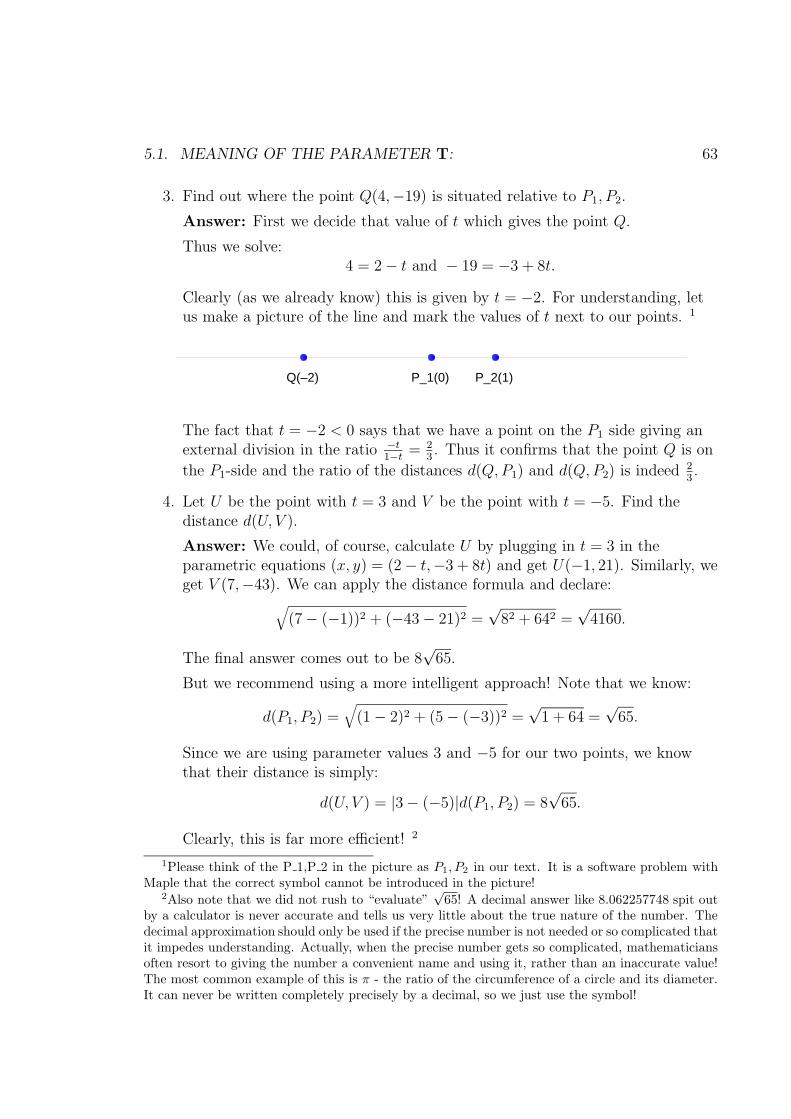
5.1. MEANING OF THE PARAMETER T: 63
3. Find out where the point Q(4,−19) is situated relative to P1, P2.
Answer: First we decide that value of t which gives the point Q.
Thus we solve:4 = 2 − t and − 19 = −3 + 8t.
Clearly (as we already know) this is given by t = −2. For understanding, letus make a picture of the line and mark the values of t next to our points. 1
Q(–2) P_1(0) P_2(1)
The fact that t = −2 < 0 says that we have a point on the P1 side giving anexternal division in the ratio −t
1−t= 2
3. Thus it confirms that the point Q is on
the P1-side and the ratio of the distances d(Q, P1) and d(Q, P2) is indeed 23.
4. Let U be the point with t = 3 and V be the point with t = −5. Find thedistance d(U, V ).
Answer: We could, of course, calculate U by plugging in t = 3 in theparametric equations (x, y) = (2 − t,−3 + 8t) and get U(−1, 21). Similarly, weget V (7,−43). We can apply the distance formula and declare:
√
(7 − (−1))2 + (−43 − 21)2 =√
82 + 642 =√
4160.
The final answer comes out to be 8√
65.
But we recommend using a more intelligent approach! Note that we know:
d(P1, P2) =√
(1 − 2)2 + (5 − (−3))2 =√
1 + 64 =√
65.
Since we are using parameter values 3 and −5 for our two points, we knowthat their distance is simply:
d(U, V ) = |3 − (−5)|d(P1, P2) = 8√
65.
Clearly, this is far more efficient! 2
1Please think of the P 1,P 2 in the picture as P1, P2 in our text. It is a software problem withMaple that the correct symbol cannot be introduced in the picture!
2Also note that we did not rush to “evaluate”√
65! A decimal answer like 8.062257748 spit outby a calculator is never accurate and tells us very little about the true nature of the number. Thedecimal approximation should only be used if the precise number is not needed or so complicated thatit impedes understanding. Actually, when the precise number gets so complicated, mathematiciansoften resort to giving the number a convenient name and using it, rather than an inaccurate value!The most common example of this is π - the ratio of the circumference of a circle and its diameter.It can never be written completely precisely by a decimal, so we just use the symbol!

64 CHAPTER 5. EQUATIONS OF LINES IN THE PLANE.
5. Use the parametric form of the above line to verify that the point S(−1, 20) isnot on it.
Answer:
We try to solve:−1 = 2 − t , 20 = −3 + 8t.
The first equation gives t = 3 and when substituted in the second equation, weget:
20 = −3 + 8(3) = 21 a clearly wrong equation!.
This shows that the point S is outside the line!
5.2 Details of the equation of a line.
The parametric description of a line given above is very useful to generate lots ofconvenient points on a line, but if we wish to understand the position and theorientation of a line as well as its intersections with other lines and curves, we needthe usual equation of a line as a relation between its x, y coordinates.We start with the parametric equations of a line thru points P1(a1, b1), P2(a2, b2)
Equation 1: x = a1 + t(a2 − a1) , Equation 2: y = b1 + t(b2 − b1)
and we construct a new equation (a2 − a1)(Equation 2) − (b2 − b1)(Equation 1).This eliminates t and we get:
(a2 − a1)y − (b2 − b1)x = (a2 − a1)b1 − (b2 − b1)a1 = (a2b1 − a1b2).
This clearly describes the precise condition that a point (x, y) lies on the line. Werecord this as:The two point form of the equation of a line thru P1(a1,b1),P2(a2,b2):
(a2 − a1)y − (b2 − b1)x = (a2b1 − a1b2).
If a2 = a1 then it is easy to see that the equation reduces to x = a1 a vertical line.Similarly, if b2 = b1, then we get a horizontal line.Example.Thus for our points P1(2,−3), P2(1, 5) we get:
(1 − (2))y − (5 − (−3))x = ((1)(−3) − (2)(5) or − y − 8x = −13 or y + 8x = 13.
You can also verify the elimination of t from the equations
x = 2 − t , y = −3 + 8t.

5.2. DETAILS OF THE EQUATION OF A LINE. 65
We now define the slope of a line joining any two points P1(a1, b1), P2(a2, b2) as
the ratio m = b2 − b1a2 − a1
where we agree that it is ∞ in case a1 = a2 i.e. when we have
a vertical line.We also define the intercepts of a line as follows:We declare:
• The x-intercept is a number a if (a, 0) is on the line.
• This may fail if the line is horizontal but not the x-axis. In other words, it failsexactly when b2 = b1 but a1b2 6= a2b1. In this case the intercept is declared ∞.
• For the x-axis itself, it is considered undefined!
• Thus, in general, the x-intercept is a2b1 − a1b2b1 − b2
with a suitable agreement
when the denominator is zero.
Similarly:
• The y-intercept is similarly defined as b, when the point (0, b) is on the line,with a suitable understanding for a vertical line.
• If a2 = a1 but a1b2 6= a2b1, i.e. if the line is vertical but not the y axis then theintercept is declared to be ∞.
• For the y-axis itself, it is considered undefined!
• In general, the formula is: a2b1 − a1b2a2 − a1
with a suitable agreement when the
denominator is zero.
For a non vertical line, it is customary to divide the equation by a2 − a1 andrewrite it as:
y − b2 − b1
a2 − a1x =
a2b1 − a1b2
a2 − a1.
The last form above is often further rearranged as: Slope intercept form of aline:
y = mx + c where m =b2 − b1
a2 − a1
is the slope and c =a2b1 − a1b2
a2 − a1
y-intercept.
Thus, for our line thru P1(2,−3),P2(1, 5), we have:
−y − 8x = −13 becomes y + 8x = 13 and finally y = −8x + 13.
Thus, the slope is −8 and intercept is 13. We can calculate each of these quantitiesfrom the formulas and then write the equation directly.

66 CHAPTER 5. EQUATIONS OF LINES IN THE PLANE.
It is convenient to understand the orientation of such a line y = mx + c.If we fix c, then we get the family of lines with a common point (0, c). When m = 0the line is horizontal and as m increases, the line starts to twist upwards (in acounter clockwise direction). Higher and higher values of m bring it closer tovertical, the true vertical being reserved for m = ∞ by convention. All these linesappear to rise as the x-coordinates increase.If we, in turn start to run m thru negative values to −∞, then the line twistsclockwise with m = −∞ corresponding to a vertical line. These lines appear to fallas x-coordinate increases.
A(02)
Slope 0
Slope 1
Slope 2Slope –2
While the above two point formula is good in all situations, sometimes it is useful tofind fast clever ways to find an equation of a line.For this, we note that any equations of the form ux + vy = w, or somethingreducible to it, is the equation of a line provided at least one of u, v is non zero.Hence, if we construct such an equation satisfying the given conditions in somefashion, it is the right answer.3
Here are some of the samples of this simple idea.Another two point form.
(y − b1)(a2 − a1) = (x − a1)(b2 − b1).
Proof: It has the right form and is clearly satisfied by the two points, justsubstitute and see!Point (P(a,b))-slope(m) form.
(y − b) = m(x − a).
Proof: When rearranged, it becomes y = mx + (b − ma).
3We may call this the “duck principle” named after the amusing saying: “If it walks like a duckand talks like a duck, then it is a duck.” Thus, if an equation looks like the equation of a line andsatisfies the required conditions, then it must be the right equation!

5.2. DETAILS OF THE EQUATION OF A LINE. 67
So, m is the slope. Also, it clearly is correct if we plug in x = a, y = b. By the way,this work also gives us the formula for the y-intercept as b − ma. The x-intercept, ifneeded is seen to be a − b/m and the evident symmetry in these two formulas isnoteworthy!Example. Find the equation of a line with slope −6 and passing thru the pointP (3, 4).Answer:
(y − 4) = −6(x − 3).
This simplifies to:y = −6x + 4 + 18 = −6x + 22.
It has slope −6 and intercept 22.Intercept form. Suppose the x, y intercepts are p, q respectively and these are nonzero. Then:
x
p+
y
q= 1.
This form can be interpreted suitably if one of p, q is zero, but fails completely ifboth are zero.Proof. Just check that the two points (p, 0), (0, q) satisfy the equation.Example. Find the equation of line with x intercept 3 and y intercept 4.Answer: Apply the formula:
x
3+
y
4= 1.
This simplifies to:
4x + 3y = 12 or y = −4
3x + 4.
Parallel lines. It is easy to see that parallel lines have the same slope. Thus a lineparallel to a given y = mx + c is given by y = mx + k where k can be chosen tosatisfy any further conditions. More generally, the line parallel to any givenux + vy = w can also be written as ux + vy = k for a suitable k. The point is thatwe don’t have to put the equation in any standard form to get it right!Example. Find a line parallel to y + 8x = 13 which passes thru the point (3, 10).Answer: We know that the answer can be of the form y + 8x = k. Impose thecondition of passing thru (3, 10), i.e.
10 + 8(3) = k
so we deduce that k = 34 and hence the answer is
y + 8x = 34.
Perpendicular lines. It is possible to prove that a line perpendicular to a linewith slope m has slope −1/m, where by convention we take 1/∞ = 0 and 1/0 = ∞.

68 CHAPTER 5. EQUATIONS OF LINES IN THE PLANE.
Thus, to make a perpendicular line to a given line of slope m, we can simply chooseany line with slope −1/m. But perhaps, we don’t wish to calculate the slope first.So, here is a general formula.A line perpendicular to ux + vy = w is given by vx − uy = k where, as before, k isto be chosen by any further conditions. For proof, it is easy to verify the slopes forthe two equations and compare.4
Example. Find a line perpendicular to y + 8x = 13 which passes thru the point(3, 10).Answer: We know that the answer can be of the form −8y + x = k. Impose thecondition of passing thru (3, 10), i.e.
−8(10) + 3 = k
so we deduce that k = −77 and hence the answer is
−8y + x = −77 or 8y − x = 77.
5.3 Examples of equations of lines.
• Points equidistant from two given points. Suppose you are given two pointsP1(a1, b1) and P2(a2, b2). Determine the equation satified by the coordinates ofa point P (x, y) equidistant from both.
Answer: We use the distance formula to write the equality of the square ofdistances from P to each of P1, P2.
(x − a1)2 + (y − b1)
2 = (x − a2)2 + (y − b2)
2.
Now expand to get:
x2 + y2 − (2a1x + 2b1y) + a21 + b2
1 = x2 + y2 − (2a2x + 2b2y) + a22 + b2
2.
Simplification leads to:
x(a1 − a2) + y(b1 − b2) = (1/2)(
(a21 − a2
2) + (b21 − b2
1))
,
where we have cancelled the terms x2, y2 and then thrown away a factor of −2before collecting terms.
4An alert reader might worry about getting different looking expressions, depending on the start-ing equation. Thus, for a starting equation of 2x+3y = 1, we can have 3x−2y = k, but 6x−4y = kseems like a valid answer as well, since our original equation could have been 4x + 6y = 2. Thepoint is that the equation of a line is never unique, since we can easily multiply it by any non zeronumber to get an equivalent equation.

5.3. EXAMPLES OF EQUATIONS OF LINES. 69
This is clearly a line and it is easy to check that it passes thru the midpoint
(a1 + a22 , b1 + b2
2 ).
The reader can also see that its slope is −a1 − a2b1 − b2
. Since the slope of the line
joining P1, P2 is b2 − b1a2 − a1
, it is obviously perpendicular to the line joining P1, P2.
Thus, we have proved that the set of points equidistant from two given pointsP1, P2 is the perpendicular bisector of the segment joining them.
Often, it is easy to use this description rather than develop the equationdirectly. Thus the locus of points equidistant from P1(1, 3), P2(3, 9) is foundthus:
The slope of the given line is 9 − 33 − 1 = 6/2 = 3. The midpoint is
((1 + 3)
2,(3 + 9)
2) = (2, 6).
Therefore, perpendicular line has slope −1/3 and hence the answer is:
(y − 6) = −(1/3)(x − 2) or y = −x/3 + 20/3.
• Right angle triangles. Given three points A, B, C, they form a right angletriangle if the Pythagorean theorem holds for the distances or equivalently twoof the sides are perpendicular.
Say, we are given points A(2, 5), B(6, 4) and wish to choose a third point Csomewhere on the line x = 4 such that ABC is a right angle triangle.
How shall we find it?
Answer: The right angle can occur at A or B or C. We can assume that thepoint C has coordinates (4, t) for some t.
If we want a right angle at A, then then the slope of the line AC times theslope of the line AB must be −1. This gives:
t − 5
4 − 2
4 − 5
6 − 2= −1 i.e. t − 5 = (−1)(4)(2)/(−1) = 8.
This gives t = 13 and C is at (4, 13).
To get a right angle at B our equation becomes:
t − 4
4 − 6
4 − 5
6 − 2= −1 i.e. t − 4 = (−1)(4)(−2)/(−1) = −8.
So we get C at (4,−4).
A similar equation for right angle at C leads to:

70 CHAPTER 5. EQUATIONS OF LINES IN THE PLANE.
t − 5
4 − 2
t − 4
4 − 6= −1 or (t − 5)(t − 4) = (−1)(2)(−2) i.e. t2 − 9t + 20 = 4.
This leads to two solutions 9 ±√
172 .

Chapter 6
The Circle
A circle is one of the most studied geometric figures. It is defined as the locus of allpoints which keep a fixed distance r (called the radius) from a given point P (a, b)called the center. 1
The distance formula leads to a simple equation:√
(x − a)2 + (y − b)2 = r, but sinceit is not easy to work with the square root, we square the equation and simplify:
(x − a)2 + (y − b)2 = r2 or x2 + y2 − 2ax − 2by = r2 − a2 − b2.
Recognizing a circle. In general, the equation of a circle can be put in the formx2 + y2 + ux + vy = w and we can then read off the center and the radius bycomparison:
u = −2a , v = −2b , w = r2 − (a2 + b2).
This gives us that the center must be (a, b) = (−u/2,−v/2).
Also, r2 = w + (a2 + b2), so r2 = w + u2/4 + v2/4 and hence the radius must be
r =√
w + u2/4 + v2/4.
What happens if the quantity w + u2/4 + v2/4 is negative or zero? We get a circlewhich has no points ( i.e. is imaginary) or reduces to a single point (−u/2,−v/2).
Consider, for example the equation x2 + y2 + 2x + 2y = k and argue that for k < −2we get a circle with no point, for k = −2 we have just the point C(−1,−1) and fork > −2 we get a circle centered at C(−1,−1) with radius
√k + 2.
1We used the traditional word locus which is a dynamic idea - it signifies the path traced by apoint moving according to the given rules; but in practice it is equivalent to the word set instead.Somehow, the locus conveys the ideas about the direction in which the points are traced and mayinclude the idea of retracing portions of the curve.
71
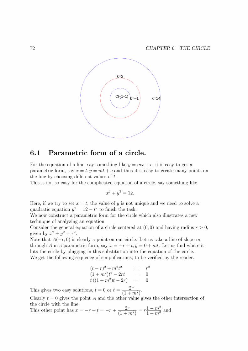
72 CHAPTER 6. THE CIRCLE
C(–1–1)
k=2
k=–1 k=14
6.1 Parametric form of a circle.
For the equation of a line, say something like y = mx + c, it is easy to get aparametric form, say x = t, y = mt + c and thus it is easy to create many points onthe line by choosing different values of t.This is not so easy for the complicated equation of a circle, say something like
x2 + y2 = 12.
Here, if we try to set x = t, the value of y is not unique and we need to solve aquadratic equation y2 = 12 − t2 to finish the task.We now construct a parametric form for the circle which also illustrates a newtechnique of analyzing an equation.Consider the general equation of a circle centered at (0, 0) and having radius r > 0,given by x2 + y2 = r2.Note that A(−r, 0) is clearly a point on our circle. Let us take a line of slope mthrough A in a parametric form, say x = −r + t, y = 0 + mt. Let us find where ithits the circle by plugging in this substitution into the equation of the circle.We get the following sequence of simplifications, to be verified by the reader.
(t − r)2 + m2t2 = r2
(1 + m2)t2 − 2rt = 0t ((1 + m2)t − 2r) = 0
This gives two easy solutions, t = 0 or t = 2r(1 + m2)
.
Clearly t = 0 gives the point A and the other value gives the other intersection ofthe circle with the line.This other point has x = −r + t = −r + 2r
(1 + m2)= r1 − m2
1 + m2 and

6.2. TRIGONOMETRIC PARAMETRIZATION. 73
y = r 2m1 + m2 .
Thus:
(x, y) = (r1 − m2
1 + m2 , r2m
1 + m2 ).
This gives a nice parametric form for the circle with parameter m. As we takedifferent values of m we get various points of the circle.What happens to the limiting case when m is sent to infinity. Indeed for this case,the line should be replaced by the vertical line x = −r and the equation ofsubstitution gives us:
r2 + y2 = r2 which leads to y2 = 0.
This says that the only point of intersection is A(−r, 0), so it makes sense to declarethat the limiting value of the parametrization gives A(−r, 0).There is an interesting algebraic manipulation of the formula which helps in suchlimiting calculations often. We present it for a better understanding.
We rewrite the expression r1 − m2
1 + m2 by dividing both the numerator and the
denominator by m2:
r1 − m2
1 + m2 = r1
m2 − 11
m2 + 1
Now with the understanding that 1/∞ goes to 0, we can deduce the result to be
r−1
1= −r.
A similar calculation leads to:
r2m
1 + m2 = r2m
1m2 + 1
→ r0
1= 0.
6.2 Trigonometric parametrization.
There is another well known parametrization of a circle which is used in thedefinition of the trigonometric functions sin(t), cos(t) that we briefly discussedearlier. Suppose we take a circle of radius 1 centered at the origin O:
x2 + y2 = 1
We wish to arrange a parameter t such that given any point P on the circle, there isa certain parameter associated with it and given any value of the parameter t, thereis a unique point P (t) associated with it.
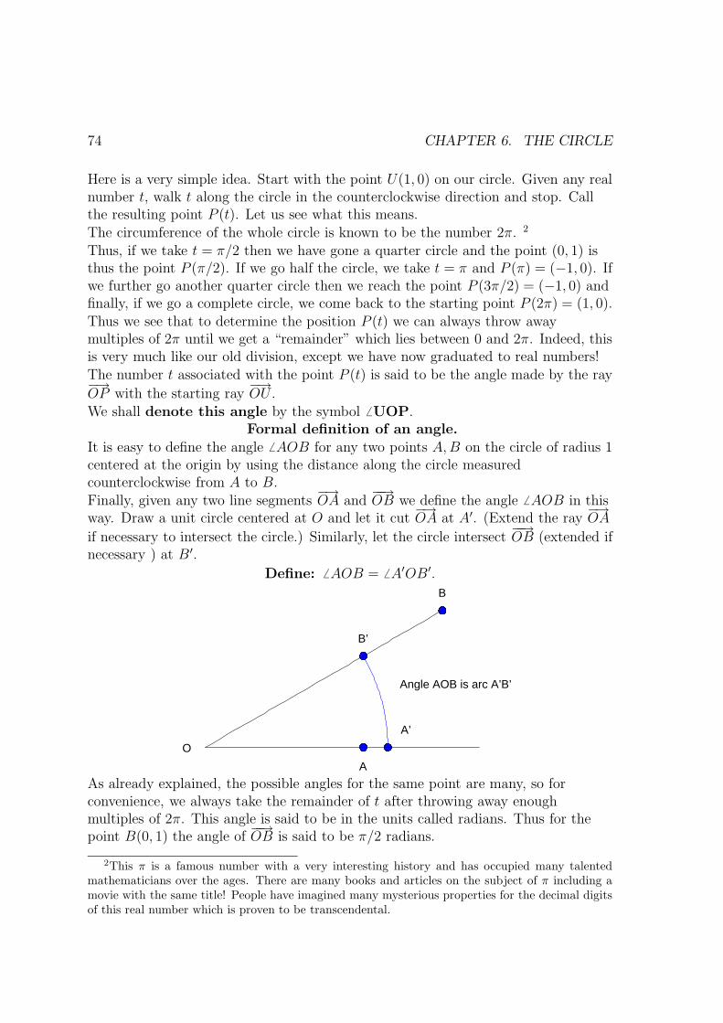
74 CHAPTER 6. THE CIRCLE
Here is a very simple idea. Start with the point U(1, 0) on our circle. Given any realnumber t, walk t along the circle in the counterclockwise direction and stop. Callthe resulting point P (t). Let us see what this means.The circumference of the whole circle is known to be the number 2π. 2
Thus, if we take t = π/2 then we have gone a quarter circle and the point (0, 1) isthus the point P (π/2). If we go half the circle, we take t = π and P (π) = (−1, 0). Ifwe further go another quarter circle then we reach the point P (3π/2) = (−1, 0) andfinally, if we go a complete circle, we come back to the starting point P (2π) = (1, 0).Thus we see that to determine the position P (t) we can always throw awaymultiples of 2π until we get a “remainder” which lies between 0 and 2π. Indeed, thisis very much like our old division, except we have now graduated to real numbers!The number t associated with the point P (t) is said to be the angle made by the ray−→OP with the starting ray
−→OU .
We shall denote this angle by the symbol 6 UOP.Formal definition of an angle.
It is easy to define the angle 6 AOB for any two points A, B on the circle of radius 1centered at the origin by using the distance along the circle measuredcounterclockwise from A to B.Finally, given any two line segments
−→OA and
−−→OB we define the angle 6 AOB in this
way. Draw a unit circle centered at O and let it cut−→OA at A′. (Extend the ray
−→OA
if necessary to intersect the circle.) Similarly, let the circle intersect−−→OB (extended if
necessary ) at B ′.
Define: 6 AOB = 6 A′OB′.
Angle AOB is arc A’B’
B’
B
A’
A
O
As already explained, the possible angles for the same point are many, so forconvenience, we always take the remainder of t after throwing away enoughmultiples of 2π. This angle is said to be in the units called radians. Thus for thepoint B(0, 1) the angle of
−−→OB is said to be π/2 radians.
2This π is a famous number with a very interesting history and has occupied many talentedmathematicians over the ages. There are many books and articles on the subject of π including amovie with the same title! People have imagined many mysterious properties for the decimal digitsof this real number which is proven to be transcendental.

6.2. TRIGONOMETRIC PARAMETRIZATION. 75
Even though this description is pleasing, it is difficult to work with, since thenumber π itself is such a mystery. In mathematical work and especially Calculus, itis important to work with radians. But forour simpler application, it is more convenient to use the more common measurecalled degrees.We simply divide the circle into 360 equal parts and call the distance correspondingto each part a degree. Thus our point B(0, 1) corresponds to the angle of 360
4= 90
degrees and it is often written as 90◦.Here is a picture of the circle with the degree measures marked at various points.
270”
180”
90”
30”
0”
45”
We now review how P (t) is determined for a given t assumed to be in degrees.We write:
t = 360n + s where 0 ≤ s < 360.
Thus s is the remainder of t after division by 360 and we mark off s degrees in ourcircle (in the counterclockwise manner) to locate the point P (t) = P (s).Thus, for t = 765 we see that t = 360(2) + 45 so s = 45 and the corresponding pointis the point at the tip of the ray making the 45 degree angle.Note that for t = −1035, we get the same s since −1035 = 360(−3) + 45.For the reader’s convenience we present a table of the corresponding angle measuresof the marked points in our picture.
degrees 0 30 45 90 180 270radians 0 π/6 π/4 π/2 π 3π/2
In the remaining work, we shall use the degree notation ◦ when we use degrees, butwhen we mean to use radians, we may skip any notation or mention of units!Definition of the Trigonometric Functions.Given an angle t, we now know how to find the associated point P (t) and so weknow its x and y coordinates. Write
P (t) = (x(t), y(t)).
76 CHAPTER 6. THE CIRCLE
Then the definition of the trigonometric functions is:
sin(t) = y(t) and cos(t) = x(t).

6.2. TRIGONOMETRIC PARAMETRIZATION. 77
Before proceeding, let us calculate a bunch of these values.Some trigonometric values.
1. Find the values of cos(0), sin(0).
Answer: When the angle 6 UOP is 0, our point P is the same as U(1, 0). Soby definition,
cos(0) = 1, sin(0) = 0.
2. Find the values of cos(90◦), sin(90◦).
Answer: We already know this point P (90◦) to be (0, 1), so we get:
cos(90◦) = 0, sin(90◦) = 1.
The reader can verify the values for 180◦ and 270◦ just as easily. They are:
cos(180◦) = −1 , sin(180◦) = 0
andcos(270◦) = 0 , sin(270◦) = −1.
3. Find the values of cos(30◦), sin(30◦).
Answer: This needs some real work! We shall give a shortcut later.
Let us make a triangle 4OMP where P is the point at 30◦ and M is the footof the perpendicular from P onto the
−→OU .
We show a picture below where we have added the midpoint H of OP and theline HM joining it with M .
H
M
P(30”)
OU
A little geometric argument can be used to deduce that
d(H, O) = d(H, M) = d(H, P )
and then the triangle 4HMP is equilateral. This says that
78 CHAPTER 6. THE CIRCLE
d(M, P ) = d(H, P ) =1
2d(O, P ) =
1
2.
Thus, we have given a brief idea of how to figure out that
sin(30◦) =1
2.
How to find cos(30◦)? We can now use simple algebra using the fact that thepoint P (30◦) is on the circle x2 + y2 = 1. So,
cos(30◦)2 + (1
2)2 = 1
and it is easy to deduce that
cos(30◦)2 = 1 − 1
4=
3
4.
It follows that
cos(30◦) = ±√
3
4= ±
√3
2.
Which sign shall we take? Clearly, from the picture, the x-coordinate ispositive, so we get
cos(30◦) =
√3
2.
Bonus thought! What do we get if we take the minus sign? After a littlethought, you can see that the angle of 180 − 30 = 150 degrees will have thesame sin, namely 1
2and its cos will be indeed −
√3
2.
Similarly, for the angle −30◦ which is also the angle 330◦, you can see that
sin(−30◦) = −1
2and cos(−30◦) =
√3
2.
We will give general formulas like this later.
We shall not pursue this much further here, but want to illustrate that with amore generous idea of parametrization, one can handle difficult calculations,although it may require more ingenuity!
We shall, however, state a fundamental formula (without proof) which can beused for algebraic calculations of sine, cosine functions for most interestingangles.
The reader is encouraged to consult appropriate text on trigonometry forfurther guidance.

6.2. TRIGONOMETRIC PARAMETRIZATION. 79
4. Find the value of sin(13◦), cos(13◦).
Answer: There is no clever way for this calculation. All we can hope to do isto use a calculator or computer, or develop a formula which can give us betterand better approximations.
A calculator will say:
sin(13◦) = 0.2249510544 and cos(13◦) = 0.9743700648.
6.2.1 Yet another take on parametrizing the circle.
The simple identity(a − b)2 + 4ab = (a + b)2
has been used for many clever applications.First we divide it by (a + b)2 to get
(a − b)2
(a + b)2 +4ab
(a + b)2 = 1.
Replacing a by 1 and b by m2 we see that
(1 − m2
1 + m2 )2 + (2m
1 + m2 )2 = 1.
We now show how it can lead to a new explanation of the parametrization of a circle.Consider, as above the circle
x2 + y2 = r2.
Rewrite it after dividing both sides by r2 to get:
(x
r)2 + (
y
r)2 = 1
.It follows that
x = r1 − m2
1 + m2 , y = r2m
1 + m2 .
is a parametrization!We now use the above to discuss:Pythagorean triples.A Pythagorean triple is a triple of integers x, y, z such that
x2 + y2 = z2.
For convenience, one often requires all numbers to be positive. If x, y, z don’t have acommon factor, then the triple is said to be primitive.
80 CHAPTER 6. THE CIRCLE
The same original identity can also be used to generate lots of examples ofPythagorean triples.We divide the original identity by 4 and plug in a = s2, b = t2. Then we easily seethat
x =s2 − t2
2, y = st , z =
s2 + t2
2.
What is more exciting is that with a little number theoretic argument, this can beshown to give all possible primitive positive integer solutions (x, y, z).These primitive Pythagorean triples have been rediscovered often, in spite of theirknowledge for almost 2000 years. It is apparent that they have been known aroundthe world for a long time.Try generating some triples by taking suitable values for s, t. (For best results, takeodd values s > t without common factors!) For instance, we can take:
s t x y z3 1 4 3 55 1 12 5 135 3 8 15 177 5 12 35 377 3 20 21 297 1 24 7 25
What is the moral? A good identity goes a lone way!
Optional section: A brief discussion of the General conic.
A conic is a plane curve which is obtained by intersecting a cone with planes indifferent position. Study of conic sections was an important part of Greek Geometryand several interesting and intriguing properties of conics have been developed overtwo thousand years.In our algebraic viewpoint, a conic can be described as any degree two curve, i.e. acurve of the form
General conic: ax2 + by2 + 2hxy + 2fx + 2gy + c = 0.
We invite the reader to show that the above idea of parametrizing a circle worksjust as well for a conic. We simply take a point A(p, q) on the conic and consider aline x = p + t, y = q + mt. The intersection of this line with the conic gives twovalue of t, namely
t = 0 , t =−2(bqm + f + gm + ap + hpm + hq)
a + 2hm + bm2 .
The reader is invited to carry out this easy but messy calculation as an exercise inalgebra.
6.2. TRIGONOMETRIC PARAMETRIZATION. 81
It is interesting to work out the different types of the conics: circle/ellipse, parabola,hyperbola and a pair of lines. We can work out how the equations can tell us thetype of the conic and its properties. But a detailed analysis will take too long. Herewe simply illustrate how the idea of parametrization can be workied out for a givenequation.
Example of parametrization. Parametrize the parabola
y2 = 2x + 2
using the point A(1, 2).
Answer: We shall first change coordinates to bring the point A to the origin. Thisis not needed, but does simplify our work.
Thus we set x = u + 1, y = v + 2, the the point A(1, 2) gets new coordinates u = 0,v = 0. Our equation becomes:
(v + 2)2 = 2(u + 1) + 2 or v2 + 4v = 2u.
Now a line thru the origin in (u, v) coordinates is given by u = t, v = mt where m isthe slope.
Substitution gives
m2t2 + 4mt = 2t or, by simplifying t(m2t + (4m − 2)).
Thus there are two solutions t = 0, t = 2 − 4mm2 . We ignore the known solution t = 0
corresponding to our starting point A.
We use the second solution for the parametrization:
u = t =2 − 4m
m2 and v =2m − 4m2
m2 .
When we go back to the original coordinates, we get:
x = 1 +2 − 4m
m2 =m2 − 4m + 2
m2
and
y = 2 +2m − 4m2
m2 =2m − 2m2
m2 .
It is an excellent idea to plug this into the original equation and verify that theequation is satisfied for all values of m. This means that the final equation shouldbe free of m and always true!

82 CHAPTER 6. THE CIRCLE
6.3 Examples of equations of a circle.
• Intersection of two circles. Find all the points of intersections of the twocircles:
x2 + y2 = 5 , x2 + y2 − 3x − 4y + 6 = 0.
Answer: The general idea of solving two equations is to solve one for one ofthe variables, say y and then plug in the other to get an equation in theremaining variable x. Then solve the resulting equation for x and thencalculate y from the first solution.
But here, both equations are quadratic in x, y and we will run into somewhatunpleasant calculations with the square roots.
A better strategy is this: Let f = x2 + y2 − 5 and g = x2 + y2 − 3x − 4y + 6.We are looking for common zeros of f, g. It follows that any such common zerowill also be a zero of an expression uf + vg where u, v are polynomials in x, y.We try to find suitable expressions which are simpler than f, g themselves.
Thus consider:
f − g = (x2 + y2 − 5) − (x2 + y2 − 3x − 4y + 6) = 3x + 4y − 11.
Thus for any of the common points, we have 3x + 4y = 11 or y = 11−3x4
.
This is clearly better than the square root expression we would have gotten.
Plugging this into the equation f = 0 we get
x2 + (11 − 3x
4)2 − 5 = 0.
This simplifies to:
25
16x2 − 33
8x +
41
16= 0 or 25x2 − 66x + 41.
Further, it is easy to verify that it has two roots:
x = 1, x =41
25.
Plugging back into the expression for y, we get corresponding y values andhence the points are:
P (1, 2) and Q(41
25,38
25).
Actually, for intersecting two circles whose equations have the same quadraticterms (x2 + y2 for example) the process of subtracting one from the otheralways gives a nice linear condition.
Indeed, this is a short cut to the solution of the next problem.
6.3. EXAMPLES OF EQUATIONS OF A CIRCLE. 83
• Line joining the intersection points of the two circles. Find the line joiningthe common points of the two circles:
x2 + y2 = 5 , x2 + y2 − 3x − 4y + 6 = 0.
Answer: We use the “duck principle”. As before, we set f = x2 + y2 − 5 andg = x2 + y2 − 3x − 4y + 6 and note that all the common points satisfyf − g = 3x + 4y − 11 = 0.
Thus 3x + 4y − 11 = 0 contains all the common points and is evidently a line,in view of its linear form; so we have found the answer!
Note that we do not need to solve for the common points at all.Moral: Avoid work if you can!
• Circle through three given points. Find the equation of a circle through thegiven points A(0, 0), B(3, 1), C(1, 3).
Answer: We begin by assuming that the desired equation is
x2 + y2 + ux + vy = w
and write down the three equations obtained by plugging in the given points:
0 + 0 + 0 + 0 = w , 9 + 1 + 3u + v = w , 1 + 9 + u + 3v = w.
These simplify to:
w = 0 , 3u + v = w − 10 , and u + 3v = w − 10.
The reader should verify that the solution is
u = −5/2, v = −5/2, w = 0 so the equation is: x2 + y2 − 5x/2 − 5y/2 = 0.
¿From what we already know, we get that this is a circle with
center: (−u/2,−v/2) = (5/4, 5/4)
andradius:
√
w + u2/4 + v2/4 =√
50/16 = (5/4)√
2.
Here we used the known formulas. What do we do if we have forgotten them?We should learn to derive the formula as needed.
We want to rewrite
x2 + y2 − 5x/2 − 5y/2 = 0 as (x − a)2 + (y − b)2 − r2 = 0.

84 CHAPTER 6. THE CIRCLE
Expanding the desired form, we get:
x2−2ax+a2+y2−2by+b2−r2 or by rearrangement x2+y2−2ax−2by+a2+b2−r2.
Now it appears in the shape as our equation and a simple comparison ofcoefficients does the job!
• Failure to find a circle through three given points. The three equations thatwe obtained above can fail to have a solution, exactly when the three chosenpoints all lie on a common line. The reader is invited to attempt to find acircle through the points:
(0, 0), (3, 1), (6, 2)
and notice the contradiction in the resulting equations:
0 + 0 + 0 + 0 = w , 9 + 1 + 3u + v = w , 36 + 4 + 6u + 2v = w
which lead to:w = 0 , 3u + v = −10 , 6u + 2v = −40.
• Smallest circle with a given center meeting a given line. Find the circle withthe smallest radius which has center at A(1, 1) and which meets the line2x + 3y = 6.
Answer: We assume that the circle has the equation:
(x − 1)2 + (y − 1)2 = r2 with r to be determined.
We will find it convenient to use a parametric form of the line and we setx = t, y = (6 − 2x)/3 = (6 − 2t)/3 = 2 − (2/3)t.
Plugging in the circle, we get:
(t − 1)2 + (2 − (2/3)t − 1)2 = r2 which simplifies to:13
9t2 − 10
3t + 2 = r2.
In a later section, we shall show that a quadratic polynomial ax2 + bx + c witha > 0 has the smallest possible value − b2
4a+ c when x = − b
2a, so here we have
that the left hand side of our equation has the least value
−1009
4139
+ 2 = −100
52+ 2 =
−100 + 104
52=
1
13.
Thus the smallest radius is√
1/13. Note that if we take r =√
1/13 then t = 1513
gives a single point of intersection, while for any bigger value of r we get twopoints corresponding to the two solution of the quadratic equation in t.

6.3. EXAMPLES OF EQUATIONS OF A CIRCLE. 85
The above calculation can be done more efficiently thus:
A common point of the circle and the line is simply a point on the line whosedistance from the center A(1, 1) is equal to the radius r. Thus we simply wantthe smallest distance between the points on the line given in parametric formas (t, 2 − (2/3)t) and the center A(1, 1). By geometric consideration, we can
argue that this minimum must occur at a point B on the line for which−→AB is
perpendicular to the line. 3
We now take a line passing thru A(1, 1) perpendicular to the given line2x + 3y = 6 and wherever they intersect, we get the point B with minimumdistance. The line has slope −2/3, so our line
−→AB must have slope 3/2.
An easy parametric form for the line−→AB is then (1 + 2s, 1 + 3s) and plugging
this into the given equation of the line, we get:
2(1 + 2s) + 3(1 + 3s) = 6 or 2 + 3 + (4 + 9)s = 6.
This leads to s = 1/13 and the point B(1 + 2/13, 1 + 3/13) = (15/13, 16/13),the same point as above!
We summarize this as a general result and leave it to the reader to establish:
• The distance between a point and a line. Given a line L : ax + by + c = 0 anda point A(p, q), show that the point B on the line L which is closest to A isgiven by the formula
B(p − aw
a2 + b2, q − b
w
a2 + b2) where w = ap + bq + c.
The shortest distance, therefore, is given by
√
w2
a2 + b2 =|w|√
a2 + b2.
Hint: show that the line through A perpendicular to L can be parametrizedas (p + as, q + bs), substitute this in the equation for L and solve for s.
You could also show that the above point B is on L and that the line joiningA with B is perpendicular to L by using slopes. Then we must have thecorrect answer!
3The argument is simply this:Suppose that there is a C different from B such that
−→AC is perpendicular to the line. Then we
have a right angle triangle 4ABC with right angle at C or−−→AB as the hypotenus. Since hypotenus
is the largest side of a right angle triangle, we have that the length of−−→AB is bigger than the length
of−→AC a contradiction!

86 CHAPTER 6. THE CIRCLE
• Half plane defined by a line. Consider a line given by 3x − 4y + 5 = 0.
Consider the points A(3, 4) and B(4, 4). Determine if they are on the same orthe opposite side of the line, without relying on a graph!
For any point P (x, y) we can evaluate the expression 3x − 4y + 5. Obviously,it evaluates to 0 on the line itself. It can be shown that it keeps a constantsign on one side of the line.
Thus at the point A, the expression evaluates to 3(3) − 4(4) + 5 = −2, whileat B we get 3(4) − 4(4) + 5 = 1. Which tells us that the two points lie on theopposite sides of the line. If we consider the origin (0, 0) which gives the value5 for the expression, we see that B and the origin lie on the same side, while Ais on the other side.
It is instructive to verify this by a careful graph and also use this idea as adouble check while working with graphs.
How should one prove the above analysis?
Suppose we have two points L, M which give values a, b for the expressionrespectively.
Then any point on the segment−−→LM is of the form tL + (1 − t)M where
0 ≤ t ≤ 1 and it is not hard the see that the expression at such a pointevaluates to ta + (1 − t)b.
Now if a, b are both positive, then clearly ta + (1 − t)b is also positive for all0 ≤ t ≤ 1. If the points were to lie on opposite sides, then one of the values oft will make the evaluation zero, and this would be a contradiction. Thus thepoints L, M must lie on the same side of the line.
We can similarly argue when both a, b are negative.
When they have opposite signs, then we can see that that the quantity bb − a
is between 0 and 1 and this value of t gives a point on the line. Thus, the linejoining L, M must intersect the line. This proves that the points lie onopposite sides of the line!
We record the above information for future use.
Let L be the line given by the equation ax + by + c = 0 as above. We naturallyhave that a, b cannot be both zero and hence
√a2 + b2 is a positive quantity.
For any point P (x, y) define the expression fL(P ) = ax + by + c.
Assume that we have points P, Q outside the line, i.e. fL(P ) 6= 0 6= fL(Q).
These points P, Q lie on the same side of the line if fL(P ) and fL(Q) have thesame sign, or, equivalently, fL(P )fL(Q) > 0.
On the other hand, they lie on the opposite sides if the expressions haveopposite signs, i.e fL(P )fL(Q) < 0.

6.3. EXAMPLES OF EQUATIONS OF A CIRCLE. 87
Moreover as we travel along the line−→PQ we get every value of the expression
from fL(P ) to fL(Q). In particular, the expression fL(A) is either a constantor strictly increases or strictly decreases.
This last fact is very important in the subject called Linear Programmingwhich discusses behavior of linear expressions on higher dimensional sets.

88 CHAPTER 6. THE CIRCLE

Chapter 7
Special study of Linear andQuadratic Polynomials.
We now pay special attention to the polynomials which occur most often inapplications, namely the linear (ax + b with a 6= 0) and the quadratic (ax2 + bx + cwith a 6= 0).
7.1 Linear Polynomials.
First, as an example, consider L(x) = 3x − 5. This can be rearranged asL(x) = 3(x − 5/3). At x = 5/3 we have L(x) = 0. If x > 5/3 thenL(x) = 3(x − 5/3) > 0 since both factors are positive. Similarly, if x < 5/3, thenL(x) = 3(x − 5/3) is negative since it is a product of a positive and a negativenumber. Thus, we see that the linear expression L(x) is zero at a single point,positive on one side of it and negative on the other. If the function were −3x + 5then the argument will be similar, except now it will be positive when x < 5/3 andnegative when x > 5/3. We summarize these arguments below. The linearpolynomials L(x) = ax + b can be written as a(x + b/a) and their behavior is veryeasy to describe.
1. Case a > 0 If x has value less than −b/a then x + b/a is negative and henceL(x) = a(x + b/a) is also negative. At x = −b/a, the expression becomes 0and it becomes positive thereafter. The expression steadily increases fromlarge negative values to large positive values, hitting the zero exactly once!
2. Case a < 0 This is just like above, except for x < −b/a the value of a(x + b/a)now becomes positive, it becomes 0 at x = −b/a just like before and thenbecomes negative for x > −b/a. Thus, the expression steadily decreases fromlarge positive values to large negative values, hitting zero exactly once!
89
90CHAPTER 7. SPECIAL STUDY OF LINEAR AND QUADRATIC POLYNOMIALS.
3. Recommended analysis. In spite of the theory above, the best way to handle aconcrete expression goes something like this. Say, we have to analyze thebehavior of L(x) = −4x + 8. Find out where it is zero, i.e. solve −4x + 8 = 0.This gives x = 8/4 = 2. Thus it will have a certain sign for x < 2 and acertain sign for x > 2. How do we find them? Just test any convenient points.Say the point x = 0 has value less than 2. The evaluationL(0) = −4(0) + 8 = 8 gives a positive number. So we conclude that
L(x) is positive for x < 2.
Similarly, to test x > 2, try x = 3 and note that L(3) = −4(3) + 8 = −4 < 0.So we conclude that
L(x) is negative for x > 2.
You may be wondering about why we bothered developing the theory if allwe have to do is to check a few points. The reason is that without the theory,we would not know which and how many points to try and why should wetrust the conclusion. If we understand the theory, we can handle morecomplicated functions as well. We illustrate this with the quadraticpolynomials next.
7.2 Factored Quadratic Polynomial.
If the quadratic expression Q(x) = ax2 + bx + c could be written in factored forma(x − u)(x − v) where u ≤ v then we can easily make a similar analysis dependingon the sign of a. Interval notation. Given real numbers a < b we shall use thefollowing standard convention.
Values of x Notationa < x and x < b (a, b)a ≤ x and x < b [a, b)a < x and x ≤ b (a, b]a ≤ and x ≤ b [a, b]
A simple way to remember these is to note that we use open parenthesis when theend point is not included, but use a closed bracket if it is! The notation is oftenextended to allow a to be −∞ or b to be ∞. Thus (−∞, 4) denotes all real numbersx such that −∞ < x < 4 and it clearly has the same meaning as x < 4, since thefirst inequality is automatically true! The reader should verify the following:
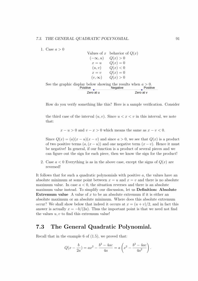
7.3. THE GENERAL QUADRATIC POLYNOMIAL. 91
1. Case a > 0Values of x behavior of Q(x)(−∞, u) Q(x) > 0x = u Q(x) = 0(u, v) Q(x) < 0x = v Q(x) = 0(v,∞) Q(x) > 0
See the graphic display below showing the results when a > 0.
Zero at u
Negative
Zero at v
Positive Positive
How do you verify something like this? Here is a sample verification. Consider
the third case of the interval (u, v). Since u < x < v in this interval, we notethat:
x − u > 0 and v − x > 0 which means the same as x − v < 0.
Since Q(x) = (a)(x − u)(x − v) and since a > 0, we see that Q(x) is a productof two positive terms (a, (x− u)) and one negative term (x− v). Hence it mustbe negative! In general, if our function is a product of several pieces and wecan figure out the sign for each piece, then we know the sign for the product!
2. Case a < 0 Everything is as in the above case, except the signs of Q(x) arereversed!
It follows that for such a quadratic polynomials with positive a, the values have anabsolute minimum at some point between x = u and x = v and there is no absolutemaximum value. In case a < 0, the situation reverses and there is an absolutemaximum value instead. To simplify our discussion, let us Definition: AbsoluteExtremum value A value of x to be an absolute extremum if it is either anabsolute maximum or an absolute minimum. Where does this absolute extremumoccur? We shall show below that indeed it occurs at x = (u + v)/2, and in fact thisanswer is actually x = −b/(2a). Thus the important point is that we need not findthe values u, v to find this extremum value!
7.3 The General Quadratic Polynomial.
Recall that in the example 6 of (1.5), we proved that:
Q(x − b
2a) = ax2 − b2 − 4ac
4a= a
(
x2 − b2 − 4ac
4a2
)
.

92CHAPTER 7. SPECIAL STUDY OF LINEAR AND QUADRATIC POLYNOMIALS.
Replacing x by x + b2a we see that:
Q(x) = a(x + b2a)2 − b2 − 4ac
4a
= az2 − b2 − 4ac4a
= a(
z2 − b2 − 4ac4a2
)
where, we have used the symbol z to denote the expression x + b2a . Note that then
x = z − b2a . If we set ∆ = b2 − 4ac
4a2 for convenience, then this expression becomes
much simpler to look at, namely:
Q(x) = a(z2 − ∆).
It is now very easy to describe its behavior. We have exactly three cases:
1. Case of ∆ < 0 or No real roots. The quantity z2 − ∆ is always positive andhence there are no real values of x which make Q(x) = 0. In this case eithera > 0 and Q(x) is always positive or a < 0 and Q(x) is always negative. Incase a > 0, the value Q(x) = a(z2 − ∆) is going to be the least exactly when
z = 0, i.e. x = z − b2a = − b
2a . Thus the minimum value −a∆ = 4ac − b2
4a is
reached at x = − b2a . In case a < 0, a similar analysis says that the maximum
value −a∆ = 4ac − b2
4a is reached at x = − b2a . Thus we have established
that x = − b2a gives an extremum value regardless of the sign of a.
Moreover, the extremum value is 4ac − b2
4a
2. Case of ∆ = 0 or a double root. In this case Q(x) = az2 = a(x + b2a)2 is a
times a complete square and becomes zero at x = − b2a . By an analysis similar
to the above, we see that x = − b2a again gives an extremum value and
the value as before is −a∆ = 0. Indeed, it is a minimum for a > 0 andmaximum for a < 0.
3. Case of ∆ > 0 or two real roots In this case Q(x) = 0 = a(z2 − ∆) leads to apair of solutions z = ±
√∆. This leads to the two roots of the original
equation x = z − b2a = ±
√∆ − b
2a . To put it in the more familiar form, we
write: The quadratic formula for solutions of ax2 + bx + c = 0, a 6= 0
x =−b ±
√b2 − 4ac
2a.
7.4. EXAMPLES OF QUADRATIC POLYNOMIALS. 93
We have done some algebraic simplification in the above formula. 1
Note that our roots u, v are simply
−b ±√
b2 − 4ac
2a
in some order and their average u + v2 is clearly
(1/2)
(
− b
2a+√
∆ − b
2a−
√∆
)
= − b
2a.
So the extremum value −b/(2a) is indeed the average of the two roots α, β. 2
7.4 Examples of quadratic polynomials.
We discuss a few exercises based on the above analysis.
1. Find the extremum values for Q(x) = 2x2 + 4x − 6 and determine interval(s)on which Q(x) is negative. Answer: We have a = 2, b = 4, c = −6. Thus
− b2a = −4
4 = −1. So, if we replace x = z − b2a = z − 1, then we have:
Q(x) = 2(z − 1)2 + 4(z − 1) − 6= 2z2 − 4z + 2 + 4z − 4 − 6= 2z2 − 8 = 2(z2 − 4)
If you remember the formula, then you can get the final answer by noticingthat
b2 − 4ac
4a2 =16 − 4(2)(−6)
4(22)=
64
16= 4.
At any rate, the value of Q(x) is clearly bigger than or equal to 2(−4) = −8and this minumum −8 is attained when z = 0 or x = z − 1 = −1. Finally, thequadratic formula (or straight factorization) will yield two rootsu = −3, v = 1. If you plot these two values on the number line you get three
1
− b
2a±√
b2 − 4ac
4a2 = − b
2a±√
b2 − 4ac/(2a).
This last simplification needs a little thought, since√
4a2 is really 2|a|, which is 2a for a > 0 and−2a for a < 0. However, because of the ± sign in front, we can just write 2a.
2Indeed, when one learns about complex numbers to find solutions of Q(x) = 0 even for negative∆, then the roots have the same formula and −b/(2a) shall still be their average. It may no longerhave any meanining of maximum or minimum value, but it is still a critical value!

94CHAPTER 7. SPECIAL STUDY OF LINEAR AND QUADRATIC POLYNOMIALS.
intervals as in our sample graph above. To check the sign of Q(x), the easiestway is to test a few strategic points as we did in the linear case.
Intervals (−∞,−3) −3 (−3, 1) 1 (1,∞)Test points −4 −3 0 1 4Values 10 0 −6 0 42Conclusion Positive Zero Negative Zero Positive
Thus, the function is negative exactly on the interval (−3, 1).
2. Find the extremum values for Q(x) = 2x2 + 4x + 6 and determine interval(s)on which Q(x) is negative. Answer: Now we have a = 2, b = 4, c = 6, so
∆ =b2 − 4ac
4a2 =16 − 4(2)(6)
4(4)= −2.
This is negative, so the theory tells us that Q(x) will have its extremum at
x = − b2a = −1 and this extremum value of Q(x) is 2(−1)2 + 4(−1) + 6 = 4.
The theory says that the expression will always keep the same positive signand so 4 is actually the minimum value and there is no maximum. There areno points where Q(x) < 0.
Chapter 8
Functions
8.1 Plane algebraic curves
The simplest notion of a plane algebraic curve is the set of all points satisying agiven polynomial equation f(x, y) = 0.We have seen that a parametric form of the description of a curve is useful forgenerating lots of points of the curve and to understand its nature.We have already learnt that all points of a line can be alternately described bylinear parametrization x = a + ut, y = b + vt for some suitable constants a, b, u, vwhere at least one of u, v is non zero.In case of a circle (or, more generally a conic) we found such a parametrization, butwith rational functions of the parameter t.Definition: A rational Curve. We say that a plane algebraic curve f(x, y) = 0is rational if it can be parametrized by rational functions.This means that we can find two rational functions x = u(t), y = v(t) such that atleast one of u(t), v(t) is not a constant and f(u(t), v(t)) is identically zero.Actually, to be precise, we can only demand that it is zero for all values of t forwhich u(t), v(t) are both defined.After the study of conics, it is tempting to think that all plane algebraic curvescould be parametrized in such a way, but alas, this is not the case. The simplestexample of a curve which cannot be parametrized by rational functions is the curvegiven by y2 = x3 − 1.1
Since we cannot hope to have all algebraic curves parametrized, we do the next bestthing; restrict our attention to the ones which are! In fact, to get a more usefultheory, we generalize of idea of an acceptable function.
1The proof that a given curve is not rational is not elementary and requires new ideas, found inadvanced books on Algebraic Geometry.
95

96 CHAPTER 8. FUNCTIONS
8.2 What is a function?
As we have seen above, a line y = 3x + 4 sets up a relation between x, y so that forevery value of x there is an associated well defined value of y, namely 3x + 4. Wemay give a name to this expression and write y = f(x) where f(x) = 3x + 4.
We wish to generalize this idea.
Definition of a function. Given two variables x, y we say that y is a function of xon a chosen domain D if for every value of x in D, there is a well defined value of y.Sometimes we can give a name to the procedure or formula which sets up the valueof y and write y = f(x).
Let us give some natural examples to illustrate this definition.
1. Polynomial functions. Let p(x) be a polynomial in x and let D be the set ofall real numbers <. Then y = p(x) is a function of x on D = <.
2. Rational functions. Let h(x) = x − 1(x − 2)(x − 3)
. Then y = h(x) has a well
defined value for every real value of x other than x = 2, 3. There is aconvenient notation for this set, namely < \ {2, 3}, which is read as “realsminus the set of 2, 3”. Let D = < \ {2, 3}. Then y = h(x) is a function of x onD.
3. Piecewise or step functions. Suppose that we define f(x) to be the integer nwhere n ≤ x < n + 1. It needs some thought to figure out the meaning of thisfunction. The reader should verify that f(x) = 0 if 0 ≤ x < 1; f(x) = 1 if1 ≤ x < 2 and so on. For added understanding, verify that f(−5.5) = −6,f(5.5) = 5, f(−23/7) = −4 and so on.
This particular function is useful and is denoted by the word floor, so insteadof f(x) we may write floor(x).
There is a similar function called ceiling or ceil for short. It is defined asceil(x) = n if n − 1 < x ≤ n.
In general, a step function is a function whose domain is split into variousintervals over which we have definitions which could be different.
A natural practical example of a step function can be something like thefollowing example.
A company charges for shipping based on the total purchase.
For purchases of up to $50, there is a flat charge of $10. For every additionalpurchase price of $10 the charge increases by $1 until the net charge is lessthan $25. If the calculation becomes $25 or higher, then shipping is free!
Describe the shipping charge function S(x) in terms of the purchace price x.

8.3. MODELING A FUNCTION. 97
Purchase price Shipping charge Commentsx ≤ 0 0 No sale!0 < x ≤ 50 10 Sale up to $50
50 < x < 200 10 + ceil(x − 5010 ) Explanation below.
200 ≤ x 0 Free shipping for big customers!
The only explanation needed is that for x > 50 the calculation of shippingcharges is 10 dollars plus a dollar for each additional purchase of up to 10dollars.
This can be analyzed thus: For x > 50 our calculation must be $10 plus theextra charge for (x − 50) dollars. This charge seems to be a 10-th of the extraamount, but rounded up to the next dollar. This is exactly the ceil functionevaluated for (x − 50)/10.
This calculation becomes 25 = 10 + 15 when x = 200 andceil((200 − 50)/10) = 15. Finally, according to the given rule we set S(x) = 0if x ≥ 200
4. Real life functions. Suppose that we define T (t) to be the temperature of somechemical mixture at time t counted in minutes. It is understood that there issome sensor inserted in the chemical and we have recorded readings at, say 10minute intervals for a total of 24 hours.
Clearly, there was a definite function with well defined values for the domain0 ≤ t ≤ (24)(60) = 1440. The domain might well be valid for a bigger set.
We have, however, no way of knowing the actual function values, withoutaccess to more readings and there is no chance of getting more readings.
What do we do?
Usually, we try to find a model, meaning an intelligent guess of a mathematicalformula (or several formulas in steps), based on the known data and perhapsknown chemical theories. We could then use Statistics to make an assertionabout our model being good or bad, acceptible or unacceptible and so on.
In this elementary course, we have no intention (or tools) to go into any suchanalysis. In the next few sections, we explain the beginning techniques of suchan analysis; at least the ones which can be analyzed by purely algebraicmethods.
8.3 Modeling a function.
We assume that we are given a small number of points in the plane and we try tofind a function f(x) of a chosen type so that the given points are on the graph of

98 CHAPTER 8. FUNCTIONS
y = f(x). Then the function f(x) is said to be a fit for the given (data) points.Here are the simplest techniques:
1. Linear fit. Given two points P1(a1, b1), P2(a2, b2) we already know how to findthe equation of a line joining them, namely(y − b1)(a2 − a1) = (x − a1)(b2 − b1), thus
y =b2 − b1
a2 − a1(x) +
b1a2 − a1b2
a2 − a1.
is the desired fit.
Of course, we know the problem when a1 = a2 and realize that having a fittingfunction with f(a1) = b1, f(a2) = b2 is then impossible anyway.
Now, if there are more than two points given and we still want to make a bestpossible linear function fit, then there is a well known formula. A fulldevelopment will take us afar, but here is a brief summary:
Optional Explanation of General Linear Fit. For the inquisitive, here arethe details, without proof. Suppose that you are given a sequence of distinctdata points (a1, b1), · · · (an, bn) where n ≥ 2, then the best fit linear function isgiven by y = mx + c where m and c are calculated by the following procedure.
Define and evaluate:
p =∑
a2 = a21 + · · · + a2
n , q =∑
a = a1 + · · ·+ an
r =∑
ab = a1b1 + · · ·+ anbn
s =∑
b = b1 + · · · bn.
Here the suggestive notations like∑
a2 are presented as an aid to memory, theexplicit formulas follow them. The greek symbol
∑
indicates a “sum” and theexpression describes a typical term.
If we take a typical pair of values x = ai, y = bi for i = 1, 2, · · · , n then we geta “wished for” equation:
bi = mai + c
and if we add this for all values of i then we get the equation s = mq + cn.
If we multiply our starting equation by ai, we get
aibi = ma2i + cai
and adding these for all values of i we get r = mp + cq.
Thus, we may think of the equations r = mp + cq and s = mq + cn as theaverage ”wish” for all the data points together.

8.3. MODELING A FUNCTION. 99
Then we solve mp + cq = r and mq + cn = s for m, c. Note that the Cramer’srule or a direct verification will give the answer:
m =nr − sq
np − q2 , c =sp − qr
np − q2 .
It is instructive to try this out for some concrete set of points and observe thatnone of the points may lie on the resulting line and the answer can besomewhat different from your intuition. However, it has a statistical andmathematical justification of being the best possible fit!
Example. Suppose that in a certain experiment we have collected thefollowing ten data points:
(1, 1), (2, 3), (3, 1), (4, 2), (5, 4), (6, 3), (7, 4), (8, 7), (9, 10), and (10, 8). Findthe best fit linear function for this data.
Answer: Noting that we have a collection of points (a1, b1),...,(a10, b10), let uscalculate the quantities p, q, r, and s as explained in the theory above.
p = 1 + 4 + 9 + 16 + 25 + 36 + 49 + 64 + 81 + 100 = 385q = 1 + 2 + 3 + 4 + 5 + 6 + 7 + 8 + 9 + 10 = 55r = 1 + 6 + 3 + 8 + 20 + 18 + 28 + 56 + 90 + 80 = 310s = 1 + 3 + 1 + 2 + 4 + 3 + 4 + 7 + 10 + 8 = 43
Now we write a proposed linear equation y = mx + c using the facts that
n = 10, m = nr − sqnp − q2 , and c = sp − qr
np − q2 .
So we have that
m =(10)(310) − (43)(55)
(10)(385) − 552 = 4955
c =(43)(385) − (55)(310)
(10)(385) − 552 = −35
The linear equation of best fit is y = 4955x − 3
5. The reader should plot the tenpoints along with the line and see how best the fit looks. This ends theoptional explanation of the General Linear Fit.
2. Quadratic fit. In general three given points will not lie on any common line.So, for a true fit, we need to use a more general function. We use a quadraticfit or a quadratic function y = q(x) = px2 + qx + r. We simply plug in thegiven three points and get three equations in the three unknowns p, q, r. Wethen proceed to solve them.
Example: Find the quadratic function that passes through the points (2, 5),(−1, 1) and (3, 7).
100 CHAPTER 8. FUNCTIONS
Answer: Let the quadratic function be 2
y = f(x) = px2 + qx + r.
Since we know that f(2) = 5, f(−1) = 1, and f(3) = 7, we can write a systemof three equations with three unknowns as follows:
5 = 4p + 2q + r1 = p − q + r7 = 9p + 3q + r.
Using methods described in previous chapters, we solve:
p =1
6, q =
7
6and r = 2.
So the quadraric function that fits the three given points is
y = f(x) =1
6x2 +
7
6x + 2.
It is good to double check that it indeed passes thru the three points.
Don’t forget that if someone gives four or more points for such a problem,then usually the precise answer may not exist. We can have a statisticalfitting answer like above, but we are not developing such general formulashere. Look up the topic of Linear Regression elsewhere.
2Don’t confuse these p, q, r with the expressions used above! They are new notations.

Chapter 9
Looking closely at a function
We have visited many functions y = f(x) where f(x) is given by a formula based ona rational function. We have also seen plane algebraic curves given by F (x, y) = 0where it is not easy to explicitly solve for y in terms of x or even to express bothx, y as nice functions of a suitable parameter.It is often possible to describe a curve near a point by nice expressions with adesired degree of accuracy and thus analyze the behavior of a function which maylack a good formula.We shall begin by discussing two simple examples.
• Analyzing a parabola.
Consider a parabola given by y = 4x2 − 2. We shall analyze it near a pointP (1, 2). Like a good investigator, we shall first go near the point by changingour origin to P .
As we know, this is easily done by the
Substitution: x = 1 + u , y = 2 + v with u, v as the new coordinates.
We shall then treat u, v as our local coordinates and the new equation as
(2 + v) = 4(1 + u)2 − 2 or v = (4(1 + 2u + u2) − 2) − 2 i.e. v = 4u2 + 8u.
Since we are studying the equation near the point u = 0, v = 0 we rewrite theequation in increasing degrees in u, v as
(v − 8u) − 4u2 = 0.
It is clear that when u, v are sufficiently small, the linear part v − 8u is goingto be much bigger than the quadratic part −4u2. We say that the linearexpression
v − 8u = y − 2 − 8(x − 1) = y − 8x + 6
101

102 CHAPTER 9. LOOKING CLOSELY AT A FUNCTION
is a Linear Approximation to the parabola near the point P (1, 2).
Alternative organization. There is a different way of doing the abovecalculation which avoids introducing new variables u, v but requires you to bemore disciplined in your work. For the reader’s convenience, we present thetechnique, which can be used as al alternative to all the following calculations.
We shall again analyze y = 4x2 − 2 at the same point (1, 2). We agree torewrite:
x as 1 + (x − 1) and y as 2 + (y − 2).
Then our parabola becomes:
2 + (y − 2) = 4(1 + (x − 1))2 − 2
which rearranges as
(y − 2) = (−2 + 4 − 2) + (4)(2)(x − 1) + 4(x − 1)2.
Thus we again get
(y − 2) = 8(x − 1) + higher degree terms in (x − 1).
and the linear approximation is again:
(y − 2) − 8(x − 1) = y − 8x − 6.
The graph below illustrates the closeness between the parabola and its linearapproximation near the point P (1, 2).
P(1,2)
The tangent line
The parabola

103
When we bring it back in the original x, y coordinates, we call the resultingline y = 8x − 6 to be the tangent line to the original parabola at P (1, 2).
Let us illustrate the same procedure with another point. Consider the pointwith x-coordinate −1. Its y-coordinate must be 4(−1)2 − 2 = 2. Shift theorigin to the point Q(−1, 2) by x = −1 + u, y = 2 + v. The equationtransforms to:
(2 + v) = 4(−1 + u)2 − 2 or v = (4(1 − 2u + u2) − 2) − 2 i.e. v = 4u2 − 8u.
1
This is rewritten in increasing degree terms as
v + 8u − 4u2 = 0.
Thus the tangent line at this point must be
v + 8u = 0 or (y − 2) + 8(x + 1) = 0 or y = −8x − 6.
Now let us do such calculations once and for all for a general point (a, b).
Naturally, we set x = a + u, y = b + v and rearrange the equation:
y = 4x2 − 2 becomes b + v = 4(a + u)2 − 2
After a little rearrangement, this becomes:
(b − 4a2 + 2) + (v − 8au) − 4u2 = 0.
Note that this final form tells us many things.
1. The point (a, b) is on our parabola if and only if the constant termvanishes. This means that b − 4a2 + 2 = 0 or b = 4a2 − 2.
2. If the point is on the parabola, then the tangent line is v − 8au = 0 orv = 8au.
In original coordinates, it becomes 2
y − b = 8a(x − a) and is rearranged to y = 8ax + (b − 8a2).
1Note that the constant term cancelled. If the constant term were to survive, it would indicatethat either the chosen point is not on the curve or that there is a mistake in the simplification.
2The line v = 8au is of interest even when the point is not on our curve. It is sometimes called apolar and has interesting properties for some special curves. Interested reader should look these upin books on algebraic geometry!
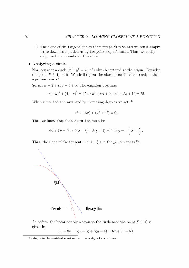
104 CHAPTER 9. LOOKING CLOSELY AT A FUNCTION
3. The slope of the tangent line at the point (a, b) is 8a and we could simplywrite down its equation using the point slope formula. Thus, we reallyonly need the formula for this slope.
• Analyzing a circle.
Now consider a circle x2 + y2 = 25 of radius 5 centered at the origin. Considerthe point P (3, 4) on it. We shall repeat the above procedure and analyze theequation near P .
So, set x = 3 + u, y = 4 + v. The equation becomes:
(3 + u)2 + (4 + v)2 = 25 or u2 + 6u + 9 + v2 + 8v + 16 = 25.
When simplified and arranged by increasing degrees we get: 3
(6u + 8v) + (u2 + v2) = 0.
Thus we know that the tangent line must be
6u + 8v = 0 or 6(x − 3) + 8(y − 4) = 0 or y = −6
8x +
50
8.
Thus, the slope of the tangent line is − 34
and the y-intercept is 254.
P(3,4)
The tangent lineThe circle
As before, the linear approximation to the circle near the point P (3, 4) isgiven by
6u + 8v = 6(x − 3) + 8(y − 4) = 6x + 8y − 50.
3Again, note the vanished constant term as a sign of correctness.

9.1. ANALYZING A GENERAL CURVE Y = F (X) NEAR A POINT (A, F (A)).105
Now we try to do this for a general point (a, b) of the circle. As before, setx = a + u, y = b + v. Substitute and rearrange the equation of the circle:
x2 + y2 − 25 = 0 becomes (a2 + b2 − 25) + 2(au + bv) + u2 + v2 = 0.
As before, we note:
1. The point (a, b) is on our circle if and only if a2 + b2 = 25.
2. If the point is on the circle, then the tangent line is au + bv = 0 after wedrop the common factor 2.
In original coordinates, it is a(x − a) + b(y − b) = 0 and rearranged toy = −a
bx + a2+b2
b. This simplifies to: y = −a
bx + 25
b.
3. The slope of the tangent line for the point (a, b) is − ab
and we couldsimply write down the equation using the point slope formula.
4. Indeed, we note that the slope of the line joining the center (0, 0) to thepoint (a, b) is b
aand hence this line is perpendicular to our tangent with
slope −ab. Thus, we have essentially proved the theorem that the radius
of a circle is perpendicular to its tangent. This, in fact, is well known forwell over 2000 years, since the time of the Greek geometry at least.
9.1 Analyzing a general curve y = f(x) near a
point (a, f(a)).
Using the experience of the parabola, let us formally proceed to analyze a generalfunction. We follow the same steps without worrying about the geometry.We state the procedure followed by a couple of examples.
1. Consider the point P (a, b) on the curve y = f(x) where, for now, we assumethat f(x) is a polynomial in x. We note that we have b = f(a).
2. Substitute x = a + u, y = b + v in y − f(x) to get b + v − f(a + u). Expandand rearrange the terms as :
(b − f(a)) + (v − lu) + ( higher degree terms in u,v ).
3. The constant term b − f(a) is zero by assumption and we declare the equationof the tangent line to y = f(x) at x = a to be the linear part set to zero:
v − lu = 0 or y − b = l(x − a) or, finally y = lx + (b − la).
106 CHAPTER 9. LOOKING CLOSELY AT A FUNCTION
We may also call it the tangent line at the point (a, f(a)) and the expressionv − lu or y − b − l(x − a) is said to be a linear approximation at this point tothe curve y − f(x).
Definition: Linear approximation to a function. We now define thelinear approximation of a function f(x) near x = a
to be simply
b + l(x − a) = lx + (b − la).
Let us note that the quantity
f(x)−f(a) = linear approximation + terms involving higher powers of (x − a)
and we could simply take this as a direct definition of a linear approximationof a function without discussing the curve y = f(x).
4. Thus we note that we only need to find the number l which can be defined asfollows:
Definition: The derivative of a polynomial function f(x) at a point a.A number l is the derivative of f(x) at x = a if f(a + u) − f(a) − lu isdivisible by u2.
Let us name the desired number l as something related to f and a and thecustomary notation is f ′(a), a quantity to be derived from f and a, or theso-called derivative of f at a.
Here are some examples of the above procedure.
1. Let f(x) = p where p is a constant. Then we have:
f(a + u) = p = f(a) + 0
so our l must be 0.
2. Let f(x) = px, where p is a constant. Then we have:
f(a + u) = p(a + u) = pa + pu = f(a) + pu
so our l is simply p.
3. f(x) = px2. Then we have:
f(a + u) = p(a + u)2 = pa2 + 2pa(u) + u2p = f(a) + 2pau + u2( more terms )
so our l is simply 2pa.
9.2. THE SLOPE OF THE TANGENT, CALCULATION OF THE DERIVATIVE.107
4. f(x) = px3. Then we have:
f(a+u) = p(a+u)3 = pa3+3pa2u+3pau2+pu3 = f(a)+2pau+u2( more terms )
so our l is simply 3pa2.
Clearly we can go on doing this, but it involves more and more calculations. Weneed to do it more efficiently. The true power of algebra consists of making a gooddefinition and recognizing a pattern!
9.2 The slope of the tangent, calculation of the
derivative.
As we know, given a function f(x) we wish to substitute a + u for x and rearrangethe expanded terms f(a + u) as f(a) + lu + higher degree terms .A more convenient notation for the derivative. We note that the parameter aused in the above analysis is just a convenient place holder and f ′(a) is really afunction of a. Hence, there is no harm in using the same letter x as a variable nameagain.Thus, for a function f(x) we will record its derivative f ′(a) as simply f ′(x). As anexample, note that our calculation for the parabola y = f(x) = 4x2 − 2 withf ′(a) = 8a can thus be recorded as f ′(x) = 8x.Finally, we introduce two shortcuts to our notation.We will find it convenient not to introduce the function name f and would like todenote the derivative directly in terms of the symbol y. We would, thus prefer towrite y′ = 8x. If the mark ′ gets confusing we shall use the notation: Dx(y) = 8x,where the symbol D denotes the word derivative and the subscript x reminds us ofthe main variable that y is a function of.Thus, our earlier results for the derivatives of pxn for n = 1, 2, 3 can be restated as
Dx(px) = p , Dx(px2) = 2x , Dx(px
3) = 3x2.
We formally declare that we shall use the notation: Dx(y) to denote the derivativef ′(x) of the function y = f(x) even though we have no explicit name f declared.
We note that there is yet another popular notation ddx
(y) or dydx
for writing the
derivative, but we will mostly use the Dx notation. 4
We begin by making some very simple observations:
4The definition looks very much like the definiton in Calculus, but our case is much simpler.In Calculus one needs to handle more complicated functions and hence needs a much more so-
phisticated analysis of the linear approximation involving the concept of limits. We shall advanceup to the derivatives of rational functions and some special functions and leave the finer details tohigher courses.
Historically, people knew the derivatives for such special functions including the trigonometricfunctions long before the formal invention of Calculus.
108 CHAPTER 9. LOOKING CLOSELY AT A FUNCTION
Formula 1 The constant multiplier.
If c is a constant and g(x) = cf(x), then g′(a) = cf ′(a).
Proof: Write f(a + u) = f(a) + f ′(a)u + u2( more terms ). Multiplying by cwe see that cf(a + u) = cf(a) + cf ′(a)u + u2( more terms ) which says thatg(a + u) = g(a) + cf ′(a)u + u2( more terms ) and hence we get g′(a) = cf ′(a).
For future understanding, let us rewrite this result as
(cf(a))′ = c(f ′(a)) or, in compact notation: Dx(cy) = cDx(y).
Formula 2 The sum of two functions. Suppose that for two functions f(x), g(x) wehave the derivatives calculated. Thus we have:
f(a + u) = f(a) + f ′(a)u + u2(· · ·) and g(a + u) = g(a) + g′(a)u + u2(· · ·).
Then we clearly have:
(f + g)(a + u) = f(a + u) + g(a + u) = f(a) + g(a) + (f ′(a) + g′(a))u + u2(· · ·).This proves that
(f + g)′(a) = f ′(a) + g′(a) or, in compact notation Dx(y + z) = Dx(y) + Dx(z).
Formula 3 The product of two functions. As above, we assume that the derivativesf ′(a), g′(a) are known. We now consider the product functionh(x) = f(x)g(x). Then we get:
h(a+u) = f(a+u)g(a+u) =[
f(a) + f ′(a)u + u2(· · ·)] [
g(a) + g′(a)u + u2(· · ·)]
.
The right hand side simplifies to:
f(a)g(a) + [f(a)g′(a) + f ′(a)g(a)] u + u2(· · ·).Thus we get the product rule:
h′(a) = (fg)′(a) = f(a)g′(a) + f ′(a)g(a)
or, in compact notation:
Dx(yz) = yDx(z) + Dx(y)z.
We illustrate the use of this formula by calculating the derivative of h(x) = x4.Write h(x) = g(x)g(x) where g(x) = x2. Note that we have alreadydetermined that g′(a) = 2a. Then by the product formula we geth′(a) = g(a)g′(a) + g′(a)g(a) = a2(2a) + (2a)a2 = 4a3. Remember, we recordthis conveniently as
h′(x) = Dx(x4) = 4x3.
We generalize this in the next formula.

9.2. THE SLOPE OF THE TANGENT, CALCULATION OF THE DERIVATIVE.109
Formula 4 The general power of x. If f(x) = xn where n = 1, 2, · · ·, thenf ′(a) = nan−1. In compact notation:
Dx(xn) = nxn−1 for n = 1, 2, · · · .
Proof. We already know this for n = 1, 2, 3, 4 from the previous section. Wenow assume that we have handled all the values of n up to some k and showhow to do the next value of k + 1. 5
Thus we assume that f(x) = xk+1 = (x)(xk) = g(x)h(x) say. By what we haveassumed, we know that g′(x) = 1 and h′(x) = kxk−1. Then the productformula gives
f ′(x) = g(x)h′(x) + g′(x)h(x) = x(kxk−1) + (1)xk = (k + 1)xk.
Thus we have proved our formula for the next value of k + 1.
We are done with the induction!
Formula 5 The combined formula. The derivative of a polynomial
f(x) = p0xn + p1x
n−1 + · · ·+ pn−1x + pn
is given by
f ′(x) = np0xn−1 + (n − 1)p1x
n−2 + · · ·+ pn−1
or in compact notation:
Dx(p0xn + p1x
n−1 + · · · + pn−1x + pn) = np0xn−1 + (n − 1)p1x
n−2 + · · ·+ pn−1.
Thus if
f(x) = 3x4 − 5x2 + x − 5
then
f ′(x) = (4)(3)x3 − (2)(5)x + 1 = 12x3 − 10x + 1.
5This is the famous method of Mathematical Induction. It gives concrete minimal argumentncessary to give a convincing proof that a statement holds for all values of integers from some pointon. There are many logically equivalent ways of organizing the argument. These different formsof the argument often reduce the task of proving a formula to just guessing the right answer andapplying the mechanical process of induction. All of our formulas for the summation of series insection 18, can be easily proved by this technique and the reader is encouraged to try this.

110 CHAPTER 9. LOOKING CLOSELY AT A FUNCTION
9.3 Derivatives of more complicated functions.
Even though we defined the derivatives only for a polynomial function so far, wehave really worked them out for even more complicated functions, without realizingit!Just consider our tangent line calculation for the circle where the explicit functionwould have involved a square root of a quadratic function! (y =
√25 − x2).
Inspired by our calculation, we shall attempt to calculate the derivative of 1x.
We begin by setting y = 1x
and simplifying it into a polynomial equation xy = 1.Following earlier practice, let us substitute x = a + u, y = b + v and simplify theresulting expression:
xy − 1 = (a + u)(b + v) − 1 = (ab − 1) + (av + bu) + (uv).
Thus the point P (a, b) is on the curve if and only if ab− 1 = 0, i.e. b = 1a
and we get:
The tangent line av + bu = a(y − b) + b(x − a) = ay + bx − 2ab = 0.
Thus the tangent line at x = a, y = 1a
is given by
ay +x
a= 2 or y =
2
a− 1
a2x.
Thus the slope of the tangent is − 1a2 and it makes sense to declare that
Dx(1
x) = Dx(x
−1) = − 1
x2= −x(−2).
The reader should note that formally, it follows the same pattern as our earlierpower formula.Would this follow the original definition of the derivative in some new sense? Yesindeed! Let us set f(x) = 1
x. Consider (and verify) these calculations:
f(a + u) =1
a + u=
1
a+
−u
a2 + au= − 1
a2· u · 1
a + u/a.
Thus, we have, after further manipulation:
f(a + u) = f(a) + (− 1
a2)u +
u2
(a + u)a2 .
The last term, is u2 times a rational function (instead of a polynomial) and it doesnot have u as a factor of the denominator. Thus we simply have to modify ourdefinition of the derivative to allow for such complications:Enhanced definition of the derivative of a rational function f(x) at a pointa. A number l is the derivative of f(x) at x = a if f(a + u) − f(a) − l(u) is equal to
9.4. MORE COMPLICATED DERIVATIVES. 111
u2 times a rational function of u which does not have u as a factor of itsdenominator.Of course, this definition is only needed as a formality; our calculation with thepolynomial equation had given the answer neatly anyway!So, let us make aFinal definition of the derivative of an algebraic function. Suppose wehave a polynomial relation f(x, y) = 0 between variables x, y. Suppose that P (a, b)is a point of the resulting curve so that f(a, b) = 0. Further, suppose that thesubstitution x = a + u, y = b + v results in a simplified form
f(a + u, b + v) = ru + sv + terms of degree 2 or more in (u, v) ,
where r, s are constants such that at least one of r, s is non zero. Then
ru + sv = r(x − a) + s(y − b)
is said to be a linear approximation of f(x, y) at x = a, y = b. The liner(x − a) + s(y − b) = 0, is defined to be the tangent line to the curve f(x, y) = 0 atP (a, b).Finally, if s 6= 0 then y can be described as a well defined algebraic function of xnear the point P (a, b) and we can define Dx(y) = − r
sor the slope of the tangent
line. In case s = 0, sometimes we may be still able to define an algebraic function,but it will not be well defined.The above paragraph leaves many details out and the interested reader inencouraged to consult higher books on algebraic geometry to learn them. The aimof the calculations and the definition is to illustrate how mathematics develops. Wedo some simple calculations which lead to possibly new ideas for functions which wedid not have before. This is how many new functions are born.
9.4 More complicated derivatives.
Armed with these new ideas, let us push our list of formulas further.
Formula 6 Enhanced power formula. Can we handle a function like y = x2
3 ? Yes,indeed.
We shall show: Dx(xn) = nxn−1 when n is any rational number. 6
Proof:7 First suppose n = pq
where p, q are positive integers. Let y = xn. Let
f(x, y) = yq − xp and note that f(x, y) = 0. We know that Dx(xp) = pxp−1, so
(a + u)p = ap + pap−1u + u2( higher degree terms in u )
6In fact, the result is true for any constant exponent, but that proof is well beyond our reach atthis point!
7The proof is easy, but messy in appearance. The student is advised to learn its use beforeworrying about the details!

112 CHAPTER 9. LOOKING CLOSELY AT A FUNCTION
Similarly, we must have Dy(yq) = qyq−1 and hence:
(b + v)q = bq + qbq−1v + v2( higher degree terms v )
It follows that
f(a + u, b + v) = (b + v)q − (a + u)p = (bq − ap) + qbq−1(v) − pap−1(u)+( terms of degree 2 or more in (u, v) ).
Thus (a, b) is a point on the curve if and only if ap = bq and the tangent line isgiven by
qbq−1(v) − pap−1(u) = 0 or qbq−1(y − b) − pap−1(x − a) = 0.
Note that since ap = bq.pap−1
qbq−1 =p
q
a−1
b−1 = nb
a.
Finally, since b = an = ap
q , we get
b
a= a
p
q−1 = an−1.
Thus the slope of the tangent is: nan−1.
In particular, we get that Dx(y) = nxn−1 as required! Our claim is thusproved for all positive fractional powers.
We now think of negative powers, i.e. we assume that y = x−n where n is apositive rational number. Set z = xn and note that yz = 1.
Our product rule (Formula 3) says that Dx(1) = yDx(z) + Dx(y)z or fromknown facts
0 = ynxn−1 + Dx(y)xn.
When solved for Dx(y), we get 8
Dx(y) =−ynxn−1
xn = −x−nnxn
xn = − n
xn .
Thus, we haveDx(x
−n) = −nx−n.
8An alert reader should seriously object at this point. We proved the product rule, but thedefinition of the derivative was only for polynomials at that time! A general product rule can beestablished, and we are not really going to do it here. We shall leave such finer details for highercourses.

9.4. MORE COMPLICATED DERIVATIVES. 113
We thus have the: General power rule.
Dx(xn) = nxn−1 where n is any rational number.
We should point out that the function xn has definition problems when x ≤ 0and our derivatives usually work only for positive x unless n is special.
Formula 7 The chain rule. We now know how to find the derivative ofg(x) = x2 + x + 1 and also we know how to find the derivative of f(x) = x5.Can we find the derivative of f(g(x)) = (x2 + x + 1)5?
Of course, we could expand it out and use our combined formula, but that isnot so pleasant!
It would be nice to have a simple mechanism to write the derivative of acomposite function. Let us work it out.
Writeg(a + u) = g(a) + lu + u2(w)
where we note that l = g′(a) and w contains remaining terms. Forconvenience, set
h = lu + u2(w),
so we get:f(g(a + u)) = f(g(a) + h)
and then by definition of the derivative of f(x) we can write
f(g(a + u)) = f(g(a)) + mh + h2(r)
where m = f ′(g(a)) and r contains the remaining terms. Note that h isdivisible by u and hence the part h2r is divisible by u2. Thus we can writeh2r = u2s for some s.
Combining terms, we write:
f(g(a + u)) = f(g(a)) + m(lu + u2w) + u2(s) = f(g(a)) + m(lu) + u2(mw + s)
and hence we deduce that the derivative of f(g(x)) at x = a is
ml = f ′(g(a))g′(a).
Thus we writeDx(f(g(x)) = f ′(g(x))g′(x).
For example, with our f(x) = x5 and g(x) = x2 + x + 1 as stated above we get
Dx((x2 + x + 1)5) = f ′(x2 + x + 1)g′(x) = 5(x2 + x + 1)4(2x + 1).
114 CHAPTER 9. LOOKING CLOSELY AT A FUNCTION
For instance, at x = 1 we have the derivative of (x2 + x + 1)5 equal to
5(1 + 1 + 1)4(2 + 1) = (5)(81)(3) = 1215
and hence the tangent line would have the equationy − (1 + 1 + 1)5 = (1215)(x − 1) simplified to y = 1215x + 243 − 1215 orfurther simplified to y = 1215x − 972.
As before, the chain rule is rather subtle to prove as our functions get morecomplicated and we need to be careful in providing its proof.
9.5 Using the derivatives for approximation.
As we discussed in the introductory section on functions, in practice, thecalculation of f(a) for a given function f(x) can be difficult and evenimpossible for real life functions given only by a few data points. If for somereason, we know the function to be linear, then obviously it is easy tocalculate its values with ease.
If a function is behaving nicely near a point, we can act as if it is a linearfunction near the point and hence can take advantage of the ease of calculation(at the cost of some accuracy, of course). In the days before calculators, manyimportant functions were often used as tables of values at equally spacedvalues of x and for values in between then, one used an ”interpolation”, i.e.guess based on the assumption that the function was linear in between.
Even when modern calculators or computers give a value of the function to adesired accuracy, they are really doing higher order versions of linearapproximations and doing them very fast; thus giving the apperance of acomplete knowledge of the function. We will illustrate some of the higherapproximations below.
Examples of linear approximations.
(a) Find an approximate value of√
3.95 using linear approximation.
Since we are discussing a square root, consider the function
f(x) =√
x = x1/2.
We know f(4) = 2 precisely. So we find a linear approximation to f(x)near x = 4.
We have already figured out that
f ′(x) = Dx(x1
2 ) =1
2x− 1
2 =1
2√
x,
9.5. USING THE DERIVATIVES FOR APPROXIMATION. 115
using the enhanced power formula.
Thus the linear approximation
L(x) = f(a) + f ′(a)(x − a) becomes
√4 + (
1
2√
4(x − 4)) or 2 +
x − 4
4.
Thus the estimated value of√
3.95 using the linear estimate is
L(3.95) = 2 +3.95 − 4
4= 1.9875.
Note that any reasonable calculator will spit out the answer 1.987460691which is certainly more accurate, but not as easy to get to! Consideringthe ease of getting a value correct to 4 decimal places, our method is welljustified!
Technically, we can use the linear approximation to calculate any desiredvalue, but clearly it only makes sense near a known good value of x.
(b) Improving a known approximation. Suppose we start with theabove approximation 1.9875 which is not quite right and its square isactually 3.95015625. Suppose we use a = 3.95015625 and thenf(a) =
√a = 1.9875. Then we get a new linear approximation
L1(x) = 1.9875 +x − 3.95015625
3.9750.
If we now set x = 3.95 and calculate the linear approximation, we get
1.9875 +3.95 − 3.95015625
3.9750= 1.987460692,
an even better value!
Thus with a repeated application of the linear approximation technique,one can get fairly accurate values. 9
Indeed, for the square root function, there is a classical algorithm knownfor over 2000 years to find successive decimal digits to any desired degreeof accuracy. This algorithm used to be routinely taught in high schoolsbefore the days of the calculators.
A similar but more complicated algorithm exists for cube roots as well.
9There are deeper issues of accumulation of roundoff errors during all calculations and reliabilityof the final conclusions. This topic is studied in the branch of mathematics called numerical analysis.

116 CHAPTER 9. LOOKING CLOSELY AT A FUNCTION
(c) Estimating polynomials: Introduction to higherapproximations. Suppose that we are trying to analyze a polynomialfunction f(x) near a point x = a. In principle, a polynomial is “easy” tocalculate precisely, but it may not be practical for a large degreepolynomial. So, we might consider approximation for it.
Let us discuss a concrete example.
Consider f(x) = 4x4 − 5x3 + 3x2 − 3x + 1. Let us take a = 1 and notethat f(a) = f(1) = 4 − 5 + 3 − 3 + 1 = 0. What is f(a + u)?
The reader should calculate:
f(x) = f(a + u) = f(1 + u) = 4u4 + 11u3 + 12u2 + 4u.
Thus for value of x near a = 1, we have u = x − 1 is small and hence thefunction f(x) can be approximated by various degree polynomials.
The Linear approximation will be 4u = 4(x − 1). The quadraticapproximation will be
12u2 + 4u = 12(x − 1)2 + 4(x − 1) = 8 − 20x + 12x2.
The cubic approximation shall be
11u3+12u2+4u = 11(x−1)3+12(x−1)2+4(x−1) = −3+13x−21x2+11x3.
The quartic (degree four) approximation will become the function itself!
Can we calculate the necessary approximations efficiently, without thewhole substitution process? The answer is yes and all we need to do is towork out some simple examples and observe. We do this next.
9.6 Efficient expansions of polynomials, the
Binomial Theorem.
Let us begin by f(x) = xn for n = 1, 2, · · · and let us try to calculate theexpansions of f(a + u). For n = 1 we simply get f(a + u) = a + u.
For n = 2 we get f(a + u) = (a + u)2 = a2 + 2au + u2.
For n = 3 we get f(a + u) = (a + u)3. Let us calculate this as follows:
(a + u)(a + u)2 = (a + u)(a2 + 2au + u)
= a(a2 + 2au + u)
+u(a2 + 2au + u)
= a3 + 2a2u + au2
+ a2u + 2au2 + u3
= a3 + 3a2u + 3au2 + u3
9.6. EFFICIENT EXPANSIONS OF POLYNOMIALS, THE BINOMIAL THEOREM.117
For n = 4 we invite the reader to do a similar calculation and deduce
(a + u)4 = (a + u)(a3 + 3a2u + 3au2 + u3)= a4 + (3a3u + a3u) + (3a2u2 + 3a2u2) + (au3 + 3au3) + u4
= a4 + 4a3u + 6a2u2 + 4au3 + u4.
Let us step back and list our conclusions.
n Coefficient list1 1 12 1 2 13 1 3 3 14 1 4 6 4 15 1 5 10 10 5 16 1 6 15 20 15 6 17 1 7 21 35 35 21 7 1
We note a pattern from first few rows, as well as recalling how we collectedthe coefficients for small values of n. The pattern is that a coefficient is thesum of the one above and the one in its northwest corner (above-left), whereany coefficient which is missing is treated as zero.
We have then boldly gone where we had not gone before and filled in the rowsfor n = 5, 6, 7. What do they tell us?
The row for n = 5 says that
(a + u)5 = (1)a5 + (5)a4u + (10)a3u2 + (10)a2u3 + (5)au4 + u5.
Notice that we start with the highest power of a, namely a5 and using thecoefficients write successive terms by reducing a power of a while increasing apower of u, until we end up in u5.
Clearly, we can continue this pattern as long as needed. This arrangement ofcoefficients is often referred to as the Pascal triangle, but it was clearly knownin China (13th century) and India (10th century or earlier). A better namewould be the Halayudha arrangement to be named after the commentator whogave it in his commentary on a very old work by Pingala in the second century.
We shall not worry about a formal proof, but the reader can use the idea ofInduction and prove the formula by the same technique.
It is more efficient to define a binomial coefficient as follows and use it whenconvenient: 10
10Why the word “binomial”? These are the coefficients coming from powers of a “two termexpression” which is called a binomial, where “bi” means two. Indeed, “poly” means many, so ourpolynomial means a many term expression.
118 CHAPTER 9. LOOKING CLOSELY AT A FUNCTION
nCr =n!
r!(n − r)!=
n(n − 1) · · · (n − r + 1)
r!.
Here, m! stands for the product (1)(2) · · · (m) for any positive integer m, witha special understanding that 0! = 1.
Why are we giving two different looking formulas, when one would do? Thefirst formula is easy to write down, but the second is easier to evaluate, sinceit has already done many of the cancellations. There is a more subtle reasonas well; the second formula can be easily evaluted when n is not even aninteger and indeed there is a famous Binomial Theorem due to Newton whichwill let you compute (1 + x)n for any power n, provided you take x small (i.e.between −1 and 1 ) and provided you get clever enough to add infinitely manyterms. We don’t get into it in this course, but we can still add many terms fora reasonable approximation!
First let us calculate a few binomial coefficients:
3C2 =3!
2!1!=
1 · 2 · 31 · 2 · 1 = 3.
Similarly,
5C3 =5!
3!2!=
1 · 2 · 3 · 4 · 51 · 2 · 3 · 1 · 2 =
3 · 4 · 51 · 2 · 3 =
2 · 51
= 10.
How do we use these? The meaning of these coefficients is that when weexpand (a + u)n and collect the terms arun−r then its coefficient is nCr.
Thus we could easily calculate the Linear approximation of f(x) = x10 asfollows.
We know that we have
f(a+u) = (a+u)10 = a10+10C1a9u+10C2a
8u2+ more terms with higher powers of u.
The value of 10C1 = 101! = 10. Note that we are using the second form of the
formula with n = 10, r = 1, so the numerator n(n − 1) · · · (n − r + 1) reducesto just 10.
Thus the linear approximation is just a10 + 10a9u = a10 + 10a9(x − a).
But, we knew this from our derivative formula as well. What is new here, isthat, in case we would like a quadratic approximation, we simply keep onemore term to write:
a10 + 10a9u +10 · 91 · 2 a8u2 = a10 + 10a9(x − a) + 45a8(x − a)2.
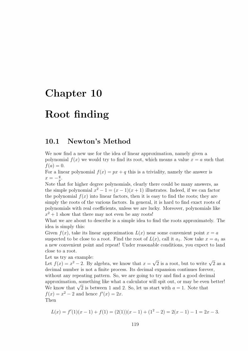
Chapter 10
Root finding
10.1 Newton’s Method
We now find a new use for the idea of linear approximation, namely given apolynomial f(x) we would try to find its root, which means a value x = a such thatf(a) = 0.
For a linear polynomial f(x) = px + q this is a triviality, namely the answer isx = − q
p.
Note that for higher degree polynomials, clearly there could be many answers, asthe simple polynomial x2 − 1 = (x − 1)(x + 1) illustrates. Indeed, if we can factorthe polynomial f(x) into linear factors, then it is easy to find the roots; they aresimply the roots of the various factors. In general, it is hard to find exact roots ofpolynomials with real coefficients, unless we are lucky. Moreover, polynomials likex2 + 1 show that there may not even be any roots!
What we are about to describe is a simple idea to find the roots approximately. Theidea is simply this:
Given f(x), take its linear approximation L(x) near some convenient point x = asuspected to be close to a root. Find the root of L(x), call it a1. Now take x = a1 asa new convenient point and repeat! Under reasonable conditions, you expect to landclose to a root.
Let us try an example:
Let f(x) = x2 − 2. By algebra, we know that x =√
2 is a root, but to write√
2 as adecimal number is not a finite process. Its decimal expansion continues forever,without any repeating pattern. So, we are going to try and find a good decimalapproximation, something like what a calculator will spit out, or may be even better!
We know that√
2 is between 1 and 2. So, let us start with a = 1. Note thatf(x) = x2 − 2 and hence f ′(x) = 2x.
Then
L(x) = f ′(1)(x − 1) + f(1) = (2(1))(x − 1) + (12 − 2) = 2(x − 1) − 1 = 2x − 3.
119
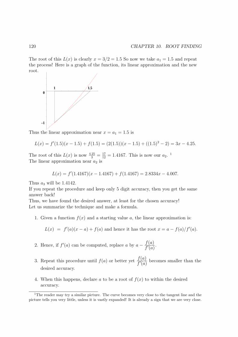
120 CHAPTER 10. ROOT FINDING
The root of this L(x) is clearly x = 3/2 = 1.5 So now we take a1 = 1.5 and repeatthe process! Here is a graph of the function, its linear approximation and the newroot.
–1
01 1.5
Thus the linear approximation near x = a1 = 1.5 is
L(x) = f ′(1.5)(x − 1.5) + f(1.5) = (2(1.5))(x − 1.5) + ((1.5)2 − 2) = 3x − 4.25.
The root of this L(x) is now 4.253
= 1712
= 1.4167. This is now our a2.1
The linear approximation near a2 is
L(x) = f ′(1.4167)(x − 1.4167) + f(1.4167) = 2.8334x − 4.007.
Thus a3 will be 1.4142.
If you repeat the procedure and keep only 5 digit accuracy, then you get the sameanswer back!
Thus, we have found the desired answer, at least for the chosen accuracy!
Let us summarize the technique and make a formula.
1. Given a function f(x) and a starting value a, the linear approximation is:
L(x) = f ′(a)(x − a) + f(a) and hence it has the root x = a − f(a)/f ′(a).
2. Hence, if f ′(a) can be computed, replace a by a − f(a)f ′(a)
.
3. Repeat this procedure until f(a) or better yetf(a)f ′(a)
becomes smaller than the
desired accuracy.
4. When this happens, declare a to be a root of f(x) to within the desiredaccuracy.
1The reader may try a similar picture. The curve becomes very close to the tangent line and thepicture tells you very little, unless it is vastly expanded! It is already a sign that we are very close.
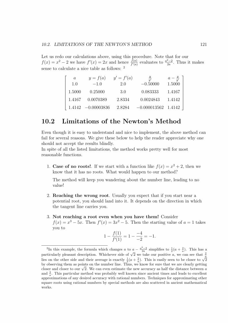
10.2. LIMITATIONS OF THE NEWTON’S METHOD 121
Let us redo our calculations above, using this procedure. Note that for ourf(x) = x2 − 2 we have f ′(x) = 2x and hence f(a)
f ′(a)evaluates to a2−2
2a. Thus it makes
sense to calculate a nice table as follows: 2
a y = f(a) y′ = f ′(a) yy′
a − yy′
1.0 −1.0 2.0 −0.50000 1.5000
1.5000 0.25000 3.0 0.083333 1.4167
1.4167 0.0070389 2.8334 0.0024843 1.4142
1.4142 −0.00003836 2.8284 −0.000013562 1.4142
10.2 Limitations of the Newton’s Method
Even though it is easy to understand and nice to implement, the above method canfail for several reasons. We give these below to help the reader appreciate why oneshould not accept the results blindly.In spite of all the listed limitations, the method works pretty well for mostreasonable functions.
1. Case of no roots!. If we start with a function like f(x) = x2 + 2, then weknow that it has no roots. What would happen to our method?
The method will keep you wandering about the number line, leading to novalue!
2. Reaching the wrong root. Usually you expect that if you start near apotential root, you should land into it. It depends on the direction in whichthe tangent line carries you.
3. Not reaching a root even when you have them! Considerf(x) = x3 − 5x. Then f ′(x) = 3x2 − 5. Then the starting value of a = 1 takesyou to
1 − f(1)
f ′(1)= 1 − −4
−2= −1.
2In this example, the formula which changes a to a − a2−22a
simplifies to 12 (a + 2
a). This has a
particularly pleasant description. Whichever side of√
2 we take our positive a, we can see that 2a
lies on the other side and their average is exactly 12 (a + 2
a). This is easily seen to be closer to
√2
by observing them as points on the number line. Thus, we know for sure that we are clearly gettingcloser and closer to our
√2. We can even estimate the new accuracy as half the distance between a
and 2a. This particular method was probably well known since ancient times and leads to excellent
approximations of any desired accuracy with rational numbers. Techniques for approximating othersquare roots using rational numbers by special methods are also scattered in ancient mathematicalworks.
122 CHAPTER 10. ROOT FINDING
Now the value a = −1 leads to
−1 − f(−1)
f ′(−1)= −1 − 4
−2= 1.
Thus you will be in a perpetual cycle between −1 and 1, never finding any ofthe roots 0,
√5,−
√5. The reader should observe that taking other values of a
does the trick. For example a = 2 takes you thru:
2 → 2.2857 → 2.2376 → 2.2361.
This is the√
5 to 5 decimal places.
Other starting values will take you to other roots.
4. Horizontal tangent. If at any stage of the process, the derivative becomeszero, then the value of the new “a” is undefined and we get stuck. For morecomplicated functions, the derivative may not even be defined! Often changingthe starting value takes care of this.
5. Accuracy problems. In addition to the above, there are possible problemswith roundoff errors of calculations both in the calculation of the derivativeand the function, problems caused by wild jumps because the derivativebecomes rather small and so y
y′gets very large!

10.2. LIMITATIONS OF THE NEWTON’S METHOD 123

124 CHAPTER 10. ROOT FINDING

Chapter 11
Summation of series.
11.1 Application of polynomials
Consider any polynomial expression f(x) and define a new polynomial
g(x) = f(x) − f(x − 1).
Consider the following sequence of substitutions.
x g(x) = f(x) − f(x − 1)1 g(1) = f(1) − f(0)2 g(2) = f(2) − f(1)· · · · · · · · · · · ·i g(i) = f(i) − f(i − 1)· · · · · · · · · · · ·n g(n) = f(n) − f(n − 1)
If we add up the g-column and equate it to the sum of the last column, we see thatmost values of f cancel leaving us with a very simple formula
g(1) + g(2) + · · ·+ g(i) + · · ·+ g(n) = f(n) − f(0).
This gives us very efficient and clever ways for adding up a series of terms.For example, let f(x) = x. Then g(x) = 1 and we get the trivial result
g(1) + · · ·+ g(n) = 1 + · · ·+ 1 = f(n) − f(0) = n − 0 = n.
If we take f(x) = x2 + x, then g(x) = 2x and we get the identity
g(1) + · · ·+ g(n) = 2 + 4 + · · ·+ 2n = f(n) − f(0) = (n2 + n) − (0) = n(n + 1).
Division of both sides by 2 gives the well known
Arithmetic series formula:1 + 2 + · · ·n =n(n + 1)
2.
125

126 CHAPTER 11. SUMMATION OF SERIES.
Thus to add up values of a gives g(x) all we have to do is to come up with a cleverlyconstructed f(x) such that g(x) = f(x) − f(x − 1). The best strategy is to try lotsof simple f(x) and learn to combine.Here is a table from simple calculations.
f(x) f(x) − f(x − 1)x 1x2 2x − 1x3 3x2 − 3x + 1x4 4x3 − 6x2 + 4x − 1x5 5x4 − 10x3 + 10x − 5x + 1
Indeed, these expressions should be deducible by using our old formulas for (x + t)n
by taking t = −1.Now suppose we wish to find the sum
12 + 22 + · · ·+ n2.
Here g(x) = x2 and we can manipulate the first three polynomials above and write
x2 = (1/3)(3x2 − 3x + 1) + (1/2)(2x − 1) + (1/6)(1)
and this tells us that f(x) = x3/3 + x2/2 + x/6 will do the trick!Thus the desired answer is:
12 + 22 + · · · + n2 = f(n) − f(0) = n3/3 + n2/2 + n/6 =(n)(n + 1)(2n + 1)
6.
Clearly, with little work, you can make your own formulas. 1
11.2 Examples of summation of series.
• Example 1: Using the idea for the Arithmetic series formula determine theformula
for the sum of n terms 2 + 5 + 8 + · · ·.Answer: This looks like adding up terms of g(x) = −1 + 3x. (Note that thisgives g(1) = 2, g(2) = 5 etc. Then g(n) = 3n − 1 and we want the formula for2 + 5 + · · ·+ (3n − 1).
By looking up our table, we see that g(x) = (3/2)(2x − 1) + (1/2), so we usef(x) = (3/2)(x2) + (1/2)(x). Indeed, check that
f(x) − f(x − 1) = (3x2 + x)/2 − ((3x2 − 5x)/2 − 1) = 3x − 1.
1It is interesting to take up the challenge of redoing the geometric series formula with this newidea. Our g(x) is now r(x−1) and the needed f(x) is to be rx/(r − 1). Verify this.

11.2. EXAMPLES OF SUMMATION OF SERIES. 127
as desired.2
• Example 2: A general arithmetic series (A.P.) 3 with beginning term a andcommon difference d is a sum of n terms a, a + d, · · · , a + (n − 1)d. Find theformula for its sum.
Answer: We can, of course work this out just as above. But to illustrate thepower of independent thinking, we shall give two other methods.
First, let us state the result to be proved.
The first method is to guess that the answer is a quadratic expression:
f(x) = px2 + qx + r.
We just try to find suitable p, q, r so the answer is correct for first few valuesof n. Here is the work.
If we take n = 0, i.e. no terms at all, then the sum must be 0, so
f(0) = p(0)2 + q(0) + r.
This says that r = 0, so f(x) = px2 + qx.
For n = 1 the sum is a and hence we want
Equation1 : f(1) = p + q = a.
For n = 2 the sum is a + (a + d) = 2a + d, so we want
Equation2 :. f(2) = p(2)2 + q(2) + r = 4p + 2q = 2a + d
To solve equations 1 and 2, we subtract twice the equation 1 from equation 2and get:
(4p + 2q) − 2(p + q) = (2a + d) − 2(a) i.e. 2p = d or p = d/2.
Using equation 1, we deduce that q = a − p = a − d/2.
2Here is a useful idea for such checking. Instead of straight substitution, first write f(x) =x(3x + 1)/2. Then f(x − 1) = (x − 1)(3(x − 1) + 1)/2 = (x − 1)(3x − 2)/2. Thus,
f(x) − f(x − 1) =x(3x + 1) − (x − 1)(3x − 2)
2=
(3x2 + x) − (3x2 − 5x + 2)
2=
6x − 2
2= 3x − 1.
3A.P. is a short form of Arithmetic Progression, which stands for the sequence of terms withcommon differences. We are using a more technical term “series” which indicates the idea of thesum of such a progression of numbers.

128 CHAPTER 11. SUMMATION OF SERIES.
Thus, we have
f(x) = dx2/2 + (a − d/2)x = x(a +x(d − 1)
2).
Hence our final answer is going to be f(n) − f(0) = f(n). This gives us:
A.P. formula An A.P. with first term a and common difference d has n-thterm as a + (n − 1)d. The sum of the first n terms is given by the expression“number of terms multiplied by the average of the first and the last terms”, i.e.
f(n) = n(a) + (a + (n − 1)d)
2.
Our second method is much cuter and easy to see, however, it does notgeneralize very well.
Let us write the terms of the A.P. in a better notation:
Let the terms be named thus:
term description valuet1 the first term at2 the second term a + dt3 the third term a + 2d· · ·tn the n-th term a + (n − 1)d
Let S(n) denote the sum t1 + t2 + · · · + tn.
Consider the following table: 4
S(n) = t1+ t2+ · · · +tn ForwardS(n) = tn+ tn−1+ · · · +t1 Reverse2S(n) = (t1 + tn)+ (t2 + tn−1)+ · · · (tn + t1) Added2S(n) = (2a + (n − 1)d)+ (2a + (n − 1)d)+ · · · (2a + (n − 1)d) Simpler!
And this last line gives the desired formula:
S(n) = (1/2)n(2a + (n − 1)d).
For example, consider the A.P. formed by 5, 8, · · ·. Here a = 5, d = 3 and then-th term is 5 + 3(n− 1) = 2 + 3n. The average of the first and the n-th termsis simply (1/2)(5 + 2 + 3n) = (7 + 3n)/2. Thus f(n) = n(7 + 3n)/2.
The reader should verify the first 10 values of this function:
5, 13, 24, 38, 55, 75, 98, 124, 153, 185.
4The main idea is that a typical i-th term is a + (i − 1)d and so i-th and (n + 1 − i)-th termsadded together give: (a + (i − 1)d) + (a + (n + 1 − i − 1)d) = 2a + (n − 1)d.
It is worth thinking about why this gives the right answer!
Chapter 12
More on the TrigonometricFunctions.
We now study more details of the trigonometric functions introduced earlier. Theaim of this section is to understand the basic definition of the various trigonometricfunctions and learn some fundamental relations governing them.
These functions, though easy to define, don’t have simple formulas and evaluatingtheir values requires careful approximations. You can use a calculator and getdecimal numbers, but that is not our goal.
We shall try to understand how these functions can be evaluated precisely for manyspecial values of the argument and how they can be manipulated formally usingalgebraic techniques. They form the basis of many mathematical theories and are,in some sense, the most important functions of modern mathematics, next topolynomials. Indeed, the theory of Fourier analysis lets us approximate all practicalfunctions in terms of suitable trigonometric functions and it is crucial to learn howto manipulate them. It is customary to also learn about exponential and logarithmicfunctions, but we have chosen to postpone it to a higher level course. Part of thereason is that their theoretical treatment requires a lot more sophistication.
As far as evaulation at specific points is concerned, trigonometric, exponential orlogarithmic functions are equally easy - they are keys on the calculator! Youprobably have already seen and used them in concrete problems anyway.
12.1 Basic definitions of Trigonometric Functions.
We shall redefine the necessary terms and make some new definitions. It would beuseful to consult the treatment of trigonometric functions in the circleparametrizations.
Definition: Angle Given two rays−→OA and
−−→OB starting from O we define the
angle from−→OA to
−−→OB thus:
129

130 CHAPTER 12. MORE ON THE TRIGONOMETRIC FUNCTIONS.
Construct a unit circle (i.e. a circle with radius 1) centered at O. Find points A′
and B′ on the rays−→OA and
−−→OB respectively, which are also on the unit circle. You
may have to extend the rays away from O so that they hit the circle.The length of the arc from A′ to B′ measured counterclockwise is the measure of theangle 6 AOB. This is the radian measure and we assume the angle to be inradians unless otherwise stated. In radian measures, the whole circle has length 2π.It is customary to use the degree measure where we let the circle have a measure of360◦.Thus to convert radians to degrees we multiply by 360
2π = 180π . Naturally, to change
degrees to radians we multiply by π180.
The angle is naturally measured as a number in the interval [0, 2π). For any realnumber t, we associate an angle s which is the remainder when the angle t isdivided by 2π.This means we write our
t = 2π(n) + s where 0 ≤ s < 2π
and n is some integer.Thus an angle of t = 9π/2 is written as
9π/2 = 4π + π/2 = 2π(2) + π/2.
Thus, even though the angle is 9π/2 for all calculations of trigonometric functionswith it, it may be safely replaced by π/2.We can do the same thing with degrees, except we divide by 360◦.Thus an angle of t = −30◦ is reduced by:
−30◦ = 360◦(−1) + 330◦
so it it declared to be equivalent to 330◦.Negative angles.Sometimes it reduces our work if we use negative values of angles, rather thatconverting them to positive angles. After all, −30◦ is easier to handle than 330◦. Wecan give a natural meaning to negative angles, they represent arc length measurethe negative or clockwise direction! Check out that going 30◦ clockwise or 330◦
counterclockwise leds to the same position!Thus, sometimes it is considered more convenient to take the angle measurebetween −180◦ to 180◦.Definition: Trigonometric functions. Given an angle t ∈ < we define P (t) asthe corresponding point on the unit circle obtained by laying off the angle t in thecounterclockwise direction as explained.We may call P (t) the locator point of the angle t. Remember that P (t) is on theunit circle centered at O and let its coordinates be (x, y).

12.2. CONNECTION WITH THE USUAL TRIGONOMETRIC FUNCTIONS.131
We define:sin(t) = x , cos(t) = y.
It is customary to define four more functions which are simply related to the abovetwo functions:
tan(t) =sin(t)
cos(t), cot(t) =
cos(t)
sin(t).
Also:
csc(t) =1
sin(t), sec(t) =
1
cos(t).
These functions have full names which are:
Notation sin cos tan cot csc secFull name Sine Cosine Tangent Cotangent Cosecant Secant
We have the following basic identities derived from the fact that P (t) is on the unitcircle.
Fundamental Identity 1. sin2(t) + cos2(t) = 1
We can divide this identity by sin2(t) or cos2(t) to derive two new identities for theother functions. The reader should verify these:
Fundamental Identity 2. 1 + cot2(t) = csc2(t)
Fundamental Identity 3. tan2(t) + 1 = cot2(t)
Remark on notation. It is customary to write sin2(t) in place of (sin(t))2. This isnot done for other functions. Indeed, many times the notation f 2(x) is use inindicate applying the function twice - i.e. f(f(x)). It is wise to verify what thisnotation means before making guesses! For trigonometric functions, this is theaccepted convention!If you have any confusion in your mind, it is safer to use the explicit (sin(t))2.The convention works for other powers too. This indeed leads to a confusion lateron if you try to use negative powers. We will explain it when it comes up.
12.2 Connection with the usual Trigonometric
Functions.
While the above definitions are precise and general, it is imporatnt to connect themwith the classical defintion.
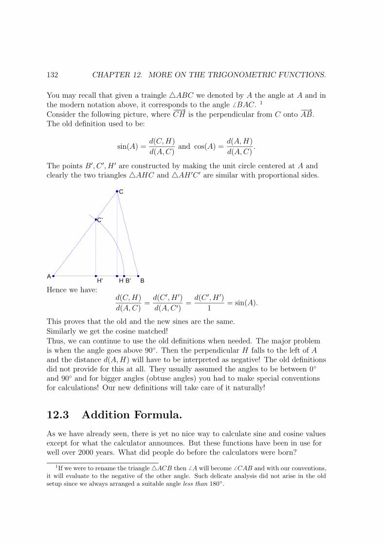
132 CHAPTER 12. MORE ON THE TRIGONOMETRIC FUNCTIONS.
You may recall that given a traingle 4ABC we denoted by A the angle at A and inthe modern notation above, it corresponds to the angle 6 BAC. 1
Consider the following picture, where−−→CH is the perpendicular from C onto
−→AB.
The old definition used to be:
sin(A) =d(C, H)
d(A, C)and cos(A) =
d(A, H)
d(A, C).
The points B′, C ′, H ′ are constructed by making the unit circle centered at A andclearly the two triangles 4AHC and 4AH ′C ′ are similar with proportional sides.
H BA
B’
C
C’
H’
Hence we have:d(C, H)
d(A, C)=
d(C ′, H ′)
d(A, C ′)=
d(C ′, H ′)
1= sin(A).
This proves that the old and the new sines are the same.
Similarly we get the cosine matched!
Thus, we can continue to use the old definitions when needed. The major problemis when the angle goes above 90◦. Then the perpendicular H falls to the left of Aand the distance d(A, H) will have to be interpreted as negative! The old definitionsdid not provide for this at all. They usually assumed the angles to be between 0◦
and 90◦ and for bigger angles (obtuse angles) you had to make special conventionsfor calculations! Our new definitions will take care of it naturally!
12.3 Addition Formula.
As we have already seen, there is yet no nice way to calculate sine and cosine valuesexcept for what the calculator announces. But these functions have been in use forwell over 2000 years. What did people do before the calculators were born?
1If we were to rename the triangle 4ACB then 6 A will become 6 CAB and with our conventions,it will evaluate to the negative of the other angle. Such delicate analysis did not arise in the oldsetup since we always arranged a suitable angle less than 180◦
.
12.3. ADDITION FORMULA. 133
The technique was to develop an addition formula - a way of computing thefunctions for a sum of two angles if we know them for each angle. This singleformula when used cleverly, lets us create a table of precise values for several anglesand then we can interpolate (intelligently guess) approximate values for otherangles. Indeed a table of 96 values was extensively used for several hundred years ofastronomy and mathematics.So, let us work on this proof.One main idea is this. Given two points P (s) and P (t) on the unit circle, it is clearthat the distance between them depends only on the difference of their angles, i.e.(t − s). This is clear since the circle is such a symmetric figure that the distancetraveled along the circle should create the same separation, no matter wher we takethe walk.Thus, we can safely conclude that
d(P (s), P (t)) = d(P (0), P (t− s)).
This is the only main point. We shall next evaluate the distance, simplify theexpression and get what we want. Before we begin, let us agree to square bothsides, since we want to avoid handling the square root in the distance formual.Note that by definition P (t) = (cos(t), sin(t)). Also note that
P (0) = (cos(0), sin(0)) = (1, 0)
from the known position of P (0).Using similar expressions for all points, we get:
(cos(t) − cos(s))2 + (sin(t) − sin(s))2 = (cos(t − s) − 1)2 + (sin(t − s) − 0)2.
Expansion and rearrangement of the left hand side (LHS) gives:
LHS = (cos2(t) + sin2(t)) + cos2(s) + sin2(s) − 2(cos(t) cos(s) + sin(t) sin(s))
Using the first fundamental identity, this simplifies to:
LHS = 1 + 1 − 2(cos(t) cos(s) + sin(t) sin(s)).
Similarly, the right hand side (RHS) becomes:
RHS = (cos2(t − s) + sin2(t − s)) + (1 + 0) − 2(cos(t − s)(1) + sin(t − s)(0)).
After simplification, it gives:
RHS = 1 + 1 − 2(cos(t − s)).
Comparing the two sides, we have our addition formula: 2
Fundamental Identity 4. cos(t − s) = cos(t) cos(s) + sin(t) sin(s)
2It appears like a subtraction formula, but it will easily become converted to the addition formulasoon!

134 CHAPTER 12. MORE ON THE TRIGONOMETRIC FUNCTIONS.
12.4 Identities Galore.
The fourth fundamental identity together with known values leads to a whole set ofnew identities. Deriving them is a fruitful fun exerise.
1. Take t = 0 in the fourth fundamental identity and write:
cos(−s) = cos(0) cos(s) + sin(0) sin(s)
and using the known values cos(0) = 1, sin(0) = 0 we get that
Evenness of the cosine function. cos(−s) = cos(s)
Note: Recall that function y = f(x) is said to be even if f(−x) = f(x) for allx in its domain. It is said to be an odd function, if, on the other handf(−x) = −f(x) for all x in the domain. Geometrically, the evenness isrecognized by the symmetry of the graph of the function about the y-axis,while the oddness is recognized by its symmetry about the origin.
2. We know that
cos(π/2) = 0 and sin(π/2) = 1.
Take t = π/2 in the fourth fundamental identity and write:
cos(π/2 − s) = (0) cos(s) + (1) sin(s) = sin(s).
Replace s by π/2 − s in this identity and get: 3
cos(π/2 − (π/2 − s)) = sin(π/2 − s).
This simplifies to
cos(s) = sin(π/2 − s).
Thus we have establishedSupplementary Angle Identity.
cos(π/2 − s) = sin(s) , sin(π/2 − s) = cos(t)
The angles s and π/2 − s are said to be supplementary angles, hence thename. Indeed, in a right angle triangle, the two angles different from the rightangle are supplementary and two positive supplementary angles arise exactlyin this way.
3If it bothers you to plug in π/2− s for s, you may do it in two steps: First replace s by π/2− zand then replace z by s.
12.4. IDENTITIES GALORE. 135
3. We proceed as above, except we now note that P (π) = (−1, 0) and take t = πin the fourth fundamental identity.
We get:
cos(π − s) = (−1) cos(s) + (0) sin(s) = − cos(s).
4. Now we replace t by π/2 − t in the fourth fundamental identity to get:
cos((π/2 − t) − s)) = cos(π/2 − t) cos(s) + sin(π/2 − s) sin(s)cos(π/2 − (t + s)) = sin(t) cos(s) + cos(s) sin(s)sin(t + s) = sin(t) cos(s) + cos(t) sin(s)
The second and third line simplifications are done using the supplementaryangle identities. We record the final conclusion as the fifth fundamentalidentity:
Fundamental Identity 5. sin(t + s) = sin(t) cos(s) + cos(t) sin(s)
5. Now take s = −t in the fifth fundamental identity to write:
sin(t − t) = sin(t) cos(−t) + cos(t) sin(−t).
Notice that the left hand side is sin(0) = 0. Since we know thatcos(−t) = cos(t) from the evenness of the cosine function, the equationbecomes:
0 = cos(t)(sin(t) + sin(−t)).
We deduce that we must have 4
Oddness of the sine function. sin(−t) = − sin(t)
6. It is worth recording the identity:
Fundamental Identity 4-variant. cos(t + s) = cos(t) cos(s) − sin(t) sin(s)
To do this, simply replace s by −s in the fundamental identity 4 and use theoddness of the sine function.
4An alert reader might object that our conclusion is not valid since we have not carefully checkedthe values of t when cos(t) = 0. This is a valid objection, but the only values of t with cos(t) = 0are given by t = ±π/2 up to multiples of 2π. Each of these cases is easily verified by hand.

136 CHAPTER 12. MORE ON THE TRIGONOMETRIC FUNCTIONS.
Armed with the fundamental identities 4 and 5, we can give a whole set of new anduseful formulas. We sketch partial argument for some and leave the rest to thereader. Indeed, it is recommended that the reader practices developing more bytrying out special cases.Here is a useful set:
1. Double angle formulas Taking s = t in the fundamental identities 4 and 5we get two important identities:
Fundamental Identity 6. cos(2t) = cos2(t) − sin2(t)
Fundamental Identity 7. sin(2t) = 2 sin(t) cos(t)
The fundamental identity 6 has two variations and they both are very useful,so we record them individually.
Fundamental Identity 6-variant 1. cos(2t) = 2 cos2(t) − 1
Fundamental Identity 6-variant 2. cos(2t) = 1 − 2 sin2(t)
These are simply obtained using the fundamental identity 1 to replace sin( t)by 1 − cos2(t) or cos2(t) by 1 − sin2(t).
2. Half Angle formulas. These are easy but powerful consequences of theabove variants of identity 6.
Fundamental Identity 8. cos(t
2) = ±
√
1 + cos(t)
2
Fundamental Identity 9. sin(t
2) = ±
√
1 − cos(t)
2
The first one is obtained by replacing t by t2 in variant 1 of identity 6. The ±
sign comes due to the square root and has to be determined by the location ofthe angle t
2.
The second one is similarly obtained from variant 2 of the identity 6.

12.4. IDENTITIES GALORE. 137
3. Using the double angle formula. Remember the complicated proof we hadto make to find the sine and cosine of 30◦?
The double and half angle formulas will make a short work of finding the sineand cosine for π
6 = 30◦ as well as π3 = 60◦.
Here is the work.
For convenience of writing, let us:
use the notation s =π
6and t =
π
3.
Notice thats + t =
π
2and t = 2s.
So by supplementary angle identity, we get
sin(t) = cos(s) and cos(t) = sin(s).
From the identity 7, we get sin(t) = 2 sin(s) cos(s) and from the above we havesin(t) = cos(s). Thus we have:
cos(s) = 2 sin(s) cos(s).
Since cos(s) clearly is non zero, we cancel it to deduce
1 = 2 sin(s) which means sin(s) =1
2.
As before, from the fundamental identity 1 we deduce that
cos(s) = ±√
1 − 1
2
2
= ±√
3
4.
And in our case we get
cos(s) =
√
3
4
due to the position of the angle in the first quadrant. We have thusestablished:
cos(60◦) = sin(30◦) =1
2and cos(30◦) = sin(60◦) =
√3
2.
Due to their frequent use, these formulas are worth memorizing!
Here is another easy but important use of the formulas.

138 CHAPTER 12. MORE ON THE TRIGONOMETRIC FUNCTIONS.
Compute the sine and cosine for π4 = 45◦.
Since 2π4 = π
2 , we see two conclusions:
sin(π
4) = cos(
π
4) and sin(
π
2) = 1 = 2 sin2(
π
4).
The reader is invited to provide the reasons. At any rate, we deduce that
sin(π
4) = cos(
π
4) =
1√2.
This formula is also worth memorizing.
4. Functions for related angles. Given one angle t, there are some anglesnaturally related to it. These are:
• Supplementary angle π/2 − t.
• Complementary angle π − t.
• Reflection at the origin π + t which is equivalent to t − π.
• reflection in the x axis −t.
We have enough tools to make our own formulas for the sine and cosinefunctions of the related angles, given those of the original angle. We leavethem as exercise.
5. What about the other functions? You might be wondering about theother four named functions we introduced, namely secant, cosecant, tangentand cotangent. We have not seen them except in the identities 2,3.
The above results for the sine and cosine functions lead to correspondingresults for them. Such results are best derived as needed, rather thanmemorized.
Thus, for example, you can deduce for yourself that sec is an even functionand that tan, cot and csc are odd functions. As a sample proof, see that:
tan(−t) =sin(−t)
cos(−t)=
− sin(t)
cos(t)= − tan(t)
where we have used the known properties of sine and cosine functions in themiddle.
There is one formula worth noting:
Fundamental Identity 10. tan(s + t) =tan(s) + tan(t)
1 − tan(s) tan(t)

12.5. USING TRIGONOMETRY. 139
The proof consists of using the identities 5 and the variant of the identity 4,together with some easy simplifications. Actually the easiest proof comes bystarting from the right hand side and simplifying. We present the stepswithout explanation:
tan(s) + tan(t)1 − tan(s) tan(t)
=
sin(s)cos(s)
+ sin(t)cos(t)
1 − sin(s) sin(t)cos(s) cos(t)
=sin(s) cos(t) + sin(t) cos(s)cos(s) cos(t) − sin(s) sin(t)
=sin(s + t)cos(s + t)
= tan(s + t)
As a consequence, we also have:
Fundamental Identity 11. tan(2t) =2 tan(t)
1 − tan2(t)
The proof is trivial, just take s = t in the identity 10. However, it is veryuseful in many theoretical calculations.
Clearly, there is no end to the kind of formulas that we can develop. There is nopoint in “learning” them all. You should learn the technique of deriving them,namely convenient substitution and algebraic manipulation.
12.5 Using trigonometry.
We shall show some of the applications of trigonometry. Like the identities, there isno end to the topics that can be added here. WE only illustrate some chosen topics.
1. Calculating exact values. So far, we have succeeded in calculating thetrigonometric functions for a few special angles 0◦, 30◦, 45◦, 60◦, 90◦ and theirrelated angles.
The half angle formula lets us evaluate many more angles.
Thus
sin(15◦) =
√
1 − cos(30◦)
2

140 CHAPTER 12. MORE ON THE TRIGONOMETRIC FUNCTIONS.
where, we have chosen the plus sign since we know the angle is in the firstquadrant. The right hand side is
√
2 −√
3
4=
√6 −
√2
4.
The last answer may be mysterious. When it is given to you, it is not hard to
check it; just square it and see that you get the desired 2 −√
34 .
There is a systematic theory of finding square roots of algebraic expressionslike this, called surds. It used to be a standard part of old algebra books; alas,no more!
It is clear that from this 15◦ angle, you can keep on halving the angle and getdown to a small angle. For several hundred years, people did their astronomyusing multiples of 7.5◦ angle.
You may ask why one should bother with this. Your calculator will happiliyreport the value 0.2588190451 for sin(15◦ as well as our theoretical value of√
6 −√
24 . You can and should use the calculator for ordinary practical
problems, but not when developing the theory. You should also have a healthysuspicion about the accuracy of the reported answer, especially if it has gonethru several steps of calculations.
2. Estimating heights. Consult the picture below for reference points.
A tall building BC is observed from the position A on the ground. The top Cof the building appears to have an elevation of 26.56◦. This means the line
−→AC
is measured to make an angle of 26.56◦ with the horizontal−→AB.
If we observe the top of the building after walking 200 feet closer to thebuilding (from point M) then it has an elevation of 32◦. Estimate the heightof the building.
M
C
BA
Answer: Even though, we are given some concrete values, the recommendedprocedure is to name everything, finish calculations and then plug in values.
Let the angles at A and M be denoted by s and t respectively. Thuss = 26.55◦ and t = 32◦. Let h be the height of the building d(B, C) and let kbe the unknown distance d(A, B). We have two equations:
12.5. USING TRIGONOMETRY. 141
E1 tan(s) =h
k
and
E2 tan(t) =h
k − 200
We wish to solve for h, k from these two equations.
Rearrangement gives:
E3. h − tan(s)k = 0 , h − tan(t)k = −200 tan(t)
Subtracting second equation in E3 from the first, we get
E4. (tan(t) − tan(s))k = 200 tan(t)
Thus
k =200 tan(t)
(tan(t) − tan(s)).
Since we really need h and not k, we use the first equation of E3 to deduce:
h = k tan(s) =200 tan(s) tan(t)
(tan(t) − tan(s)).
It remains to plug in the known angles and evaluate in a calculator. Youshould verify that it gives an answer of 499.88 feet. 5
5Some of you may be feeling that we are complicating matters too much by naming even theknown angles as s, t. You will find that the reverse is true. Try using the explicit values in theequations and then try to solve them and compare the work!
Moreover, this way, you have a wonderful formula at hand. All such height problems can now besolved by changing the various numbers in the final expression!

142 CHAPTER 12. MORE ON THE TRIGONOMETRIC FUNCTIONS.

Index
angle, 74arithmetic series, 126axes, 49axis, 49
binomial, 5binomial coefficients, 118Binomial Theorem, 116
center, 71chain rule, 114chinese remainder theorem, 35circle, 71coefficient, 3, 27complex numbers, 1conic, 80consistent, 27coordinate system, 49cos, 76cot, 131Cramer’s Rule, 21cramer’s rule, 35csc, 131
degree, 3, 27, 75degree of a polynomial, 6denominator, 65derivative, 106determinant, 35determinant of 2 by 2 matrix, 21direction numbers, 51distance, 50distance formula, 62dividend, 30divisbility of integers, 39divisibility of polynomials, 39
division, 28division algorithm, 27, 33division formula, 62divisor, 30domain, 96
ellipse, 80enhanced remainder theorem, 45euclindean algorithm, 32exponential, 129
fast calculation methods, 10field, 1Fourier analysis, 129function, 96
GCD, 31geometric series, 43, 126greatest common divisor, 31
hyperbola, 80
identity, 17inconsistent, 17, 27indeterminant, 3intercept form, 67isolating the variable, 16
LCM, 31leading coefficient of a polynomial, 6least common multiple, 31linear approximation, 102linear equation, 15linear fit, 98linear polynomial, 43logarithmic, 129
143

144 INDEX
midpoint formula, 62monic, 31monomial, 3
negative angles, 130Newton’s Method, 119numerator, 65
origin, 52
parabola, 80parallel lines, 67parameter, 2, 60parametric form, 59Pascal triangle, 117perpendicular lines, 67pi, 64plane algebraic curve, 95polynomial, 5, 27polynomial functions, 96power rule, 114Pythagorean Theorem, 51
quadrant, 51quadratic, 82quadratic fit, 99
radian, 75radius, 71range, 96rational curve, 95rational functions, 96rational numbers, 1ray, 74real number, 74real numbers, 1remainder, 28Remainder theorem, 43row echelon form, 20
sec, 131shift, 50sin, 76slope, 65, 81
slope intercept, 65solution to an equation, 16step function, 96supplementary angles, 134, 135surds, 140
tan, 131tangent line, 103the principle of 0, 1,∞ number of
solutions, 17transcendental, 74transformation, 53trigonometric functions, 130trinomial, 5
unique solution, 17unit circle, 74
Variables, 7vectors, 50
zero polynomial, 5