COLLECTIVE CLASSIFICATION OF SOCIAL NETWORK SPAM

by

JONATHAN BROPHY

A THESIS

Presented to the Department of Computer and Information Scienceand the Graduate School of the University of Oregon

in partial fulfillment of the requirementsfor the degree ofMaster of Science

June 2017

THESIS APPROVAL PAGE

Student: Jonathan Brophy

Title: Collective Classification of Social Network Spam

This thesis has been accepted and approved in partial fulfillment of therequirements for the Master of Science degree in the Department of Computer andInformation Science by:

Daniel Lowd Chair

and

Scott L. Pratt Dean of the Graduate School

Original approval signatures are on file with the University of Oregon GraduateSchool.

Degree awarded June 2017

ii

c© 2017 Jonathan Brophy

iii

THESIS ABSTRACT

Jonathan Brophy

Master of Science

Department of Computer and Information Science

June 2017

Title: Collective Classification of Social Network Spam

Unsolicited messages affects virtually every popular social media website,

and spammers have become increasingly proficient at bypassing conventional

filters, prompting a stronger effort to develop new methods. First, we build an

independent model using features that capture the cases where spam is obvious.

Second, a relational model is built, taking advantage of the interconnected

nature of users and their comments. By feeding our initial predictions from the

independent model into the relational model, we can propagate and jointly infer the

labels of all comments at the same time. This allows us to capture the obfuscated

spam comments missed by the independent model that are only found by looking

at the relational structure of the social network. The results from our experiments

shows that models utilizing the underlying structure of the social network are more

effective at detecting spam than ones that do not.

This thesis includes previously published coauthored material.

iv

CURRICULUM VITAE

NAME OF AUTHOR: Jonathan Brophy

GRADUATE AND UNDERGRADUATE SCHOOLS ATTENDED:

University of Oregon, Eugene, ORCal Poly SLO, San Luis Obispo, CA

DEGREES AWARDED:

Master of Science, Computer and Information Science, 2017, UOBachelor of Science, Electrical Engineering, 2014, Cal Poly SLO

AREAS OF SPECIAL INTEREST:

Robust Relational Machine LearningMachine Learning Interpretability

PROFESSIONAL EXPERIENCE:

Software Consultant, Asynchrony, 2015Software Developer, Macy’s, 2014

GRANTS, AWARDS AND HONORS:

Henry V. Howe Scholarship, University of Oregon, 2016

PUBLICATIONS:

Brophy, J. & Lowd, D. (2017). Collective Classification of Social NetworkSpam. Workshop on Artificial Intelligence and Cyber Security (AICS).

v

ACKNOWLEDGEMENTS

I would like to thank my advisor, Daniel Lowd, without whom this workwould not be possible. I would also like to thank Alex von Brandenfels, MichaelOdere, Zhixin Liu, and Mohsina Zaman for their contributions in this work.Finally, I would like to thank my family for their never ending support andinspiration.

vi

TABLE OF CONTENTS

Chapter Page

I. INTRODUCTION . . . . . . . . . . . . . . . . . . . . . . . . 1

II. BACKGROUND: DEFINITIONS AND TOOLKITS . . . . . . . . . 4

Random Forest . . . . . . . . . . . . . . . . . . . . . . . . . 4

SciKit-Learn . . . . . . . . . . . . . . . . . . . . . . . . . . 4

Graph Algorithms . . . . . . . . . . . . . . . . . . . . . . . 5

Pagerank . . . . . . . . . . . . . . . . . . . . . . . . . . 5

Triangle Count . . . . . . . . . . . . . . . . . . . . . . . 5

K-Core . . . . . . . . . . . . . . . . . . . . . . . . . . . 5

In-Degree . . . . . . . . . . . . . . . . . . . . . . . . . . 5

Out-Degree . . . . . . . . . . . . . . . . . . . . . . . . . 5

Graphlab . . . . . . . . . . . . . . . . . . . . . . . . . . . 5

Markov Networks . . . . . . . . . . . . . . . . . . . . . . . . 6

First Order Logic . . . . . . . . . . . . . . . . . . . . . . . . 7

Fuzzy Logic . . . . . . . . . . . . . . . . . . . . . . . . . . 7

Lukasiewicz T-Norm . . . . . . . . . . . . . . . . . . . . . 7

Hinge-Loss MRFs . . . . . . . . . . . . . . . . . . . . . . . . 8

Probabilistic Soft Logic . . . . . . . . . . . . . . . . . . . . . 8

Metrics . . . . . . . . . . . . . . . . . . . . . . . . . . . . 9

PR Curve . . . . . . . . . . . . . . . . . . . . . . . . . . 9

ROC Curve . . . . . . . . . . . . . . . . . . . . . . . . . 10

AUPR . . . . . . . . . . . . . . . . . . . . . . . . . . . 10

AUROC . . . . . . . . . . . . . . . . . . . . . . . . . . 10

vii

Chapter Page

III. RELATED WORK . . . . . . . . . . . . . . . . . . . . . . . . 11

IV. METHODOLOGY . . . . . . . . . . . . . . . . . . . . . . . . 13

Independent Model . . . . . . . . . . . . . . . . . . . . . . . 13

Content-Based Features . . . . . . . . . . . . . . . . . . . 13

Graph-Based Features . . . . . . . . . . . . . . . . . . . . 14

Relational Features . . . . . . . . . . . . . . . . . . . . . 15

Relational Model . . . . . . . . . . . . . . . . . . . . . . . . 17

Users . . . . . . . . . . . . . . . . . . . . . . . . . . . . 17

Comments . . . . . . . . . . . . . . . . . . . . . . . . . 18

Tracks . . . . . . . . . . . . . . . . . . . . . . . . . . . 20

URLs . . . . . . . . . . . . . . . . . . . . . . . . . . . 21

Weight Learning . . . . . . . . . . . . . . . . . . . . . . . 21

V. RESULTS AND ANALYSIS . . . . . . . . . . . . . . . . . . . . 23

Data . . . . . . . . . . . . . . . . . . . . . . . . . . . . . 23

Experiment Setup . . . . . . . . . . . . . . . . . . . . . . . . 24

Independent model results . . . . . . . . . . . . . . . . . . . . 26

Relational model results . . . . . . . . . . . . . . . . . . . . . 27

Increasing Model Complexity . . . . . . . . . . . . . . . . . 27

Varying Comment Datasets . . . . . . . . . . . . . . . . . . 28

Extra Observations . . . . . . . . . . . . . . . . . . . . . 30

VI. CONCLUSION . . . . . . . . . . . . . . . . . . . . . . . . . . 32

REFERENCES CITED . . . . . . . . . . . . . . . . . . . . . . . . 34

viii

LIST OF FIGURES

Figure Page

1. Sample follower graph constructed from follower actions. . . . . . . . 14

2. Relational model using predictions from an independent model aspriors in addition to user behavior to classify spam. . . . . . . . . . . 17

3. Second relational model that adds rules about matching commentsbelonging to spam or non-spam hubs. . . . . . . . . . . . . . . . . 19

4. Third relational model identifying comments belonging to spammy ornon-spammy tracks; sTrack is short for spamTrack. . . . . . . . . . . 20

5. Independent model showing performance using different featuresets. Comments used: 6 million to 8 million, tested on the last 300kcomments (left). Comments used: 38 million to 40 million, tested onthe last 300k comments (right). . . . . . . . . . . . . . . . . . . 26

6. Three relational models of increasing complexity tested on the samedata set (comments 31 million to 33 million). Model 1 with priorsand spammer information (left). Model 2 with rules added to capturematching comments (middle). Model 3 that adds rules about howspammy certain tracks are (right). . . . . . . . . . . . . . . . . . 28

7. Relational model 3 tested on three different subsets of commentsin the data. Comments used: 6 million to 8 million, tested on thelast 300k comments (left). Comments used: 31 million to 33 million,tested on the last 300k comments (Middle). Comments used: 38million to 40 million, tested on the last 300k comments (right). . . . . . 30

ix

LIST OF TABLES

Table Page

1. Features in the independent model, grouped into three differentfeature sets. . . . . . . . . . . . . . . . . . . . . . . . . . . . 15

2. Soundcloud Statistics. . . . . . . . . . . . . . . . . . . . . . . . 24

3. Independent model performance using different feature sets. AUPRscores are reported. . . . . . . . . . . . . . . . . . . . . . . . . 27

4. Comparison of different relational models to the baseline independentmodel on comments 31 million to 33 million. . . . . . . . . . . . . . 29

5. Count of different entities contained in the test set of each commentgroup (last 300k comments). . . . . . . . . . . . . . . . . . . . . 29

6. Comparison of relational model 3 on different comment datasets. . . . . 30

x

CHAPTER I

INTRODUCTION

The appearance of spam in a social network can be any instance of

unsolicited or unwanted actions by a user in the network. Traditional methods of

classifying spam have resulted in many content-based approaches that characterize

spam in messages, email, social media comments, etc. The increase in scale of

many popular social media websites has created greater incentives for spammers

to find new ways of bypassing traditional filters. Even if only a small fraction of

a spammer’s campaign gets through a spam filter, there can be a large number of

users that will see those messages, making it worthwhile for the spammer. These

spammers can avoid detection by randomizing the content of their messages, or

manipulating their content in a way that fools the content-based classifier.

An alternative method could classify spammers based on actions performed

between users in a social network Fakhraei, Foulds, Shashanka, and Getoor (2015).

This is a more robust method of detecting spammers as changing user behavior to

bypass spam filters is more difficult than altering spam messages individually. For

example, a graph structure could be built around users following other users, where

nodes represent users and directed edges represent users following other users.

Perhaps legitimate behavior is characterized by having many followers (node with

a large in-degree). Thus, a spammer might have difficulty simulating legitimate

behavior because they cannot get other users to follow them, making them easier to

find among all the other users.

By using aspects of both content and graph-based systems, a spam detection

model can capture certain signals that a system focused on only one approach

could miss. Combining these methods also gives the added benefit of finding spam

1

messages and spammers. Detecting spam messages themselves may be sufficient

for certain domains, but generally it is more useful to characterize the users that

are generating the spam to more efficiently prevent similar spam campaigns in the

future.

The combination of content and graph-based systems is an improvement,

but both of these approaches still consider the data to be independent and

identically distributed (i.i.d.). They look at incoming spam messages one at a time,

and based on characteristics about the spam message itself, as well as the user’s

previous behavior, make a decision about whether it should be labeled as spam

or not spam. Social network spam is not i.i.d. This provides the opportunity to

exploit the interconnected nature of spammers, spam comments, and any other

domain-specific entities that tie spammers to their spam.

Our approach is motivated by soundcloud.com, a social network for sharing

music. This domain is an excellent place to test out a statistical relational model

because it can exploit the underlying structure between users, messages, and

the uploaded tracks where messages are posted. Our approach uses a type of

probabilistic graphical model called hinge-loss Markov random fields (HL-MRFs)

Bach, Huang, London, and Getoor (2013) to jointly infer labels of spam messages.

The remaining chapters accomplish the following: Chapter 2 goes over

definitions, techniques, and tools necessary for this paper. Chapter 3 highlights

the most important work related to this research. Chapter 4 describes the

methodology of our approach to detecting spam. Chapter 5 reveals the results

from our experiments for the independent and relational models. Finally, Chapter 6

concludes with a short discussion and possible directions for future work.

2

Each chapter in this thesis contains coauthored material with professor

Daniel Lowd who advised the work in each chapter. This coauthored material

will be published in the proceedings of the 2017 AAAI workshop on artificial

intelligence and cyber security (AICS) under the title ’Collective Classification of

Social Network Spam’.

3

CHAPTER II

BACKGROUND: DEFINITIONS AND TOOLKITS

From Jonathan Brophy and Daniel Lowd. 2017 AAAI Workshop on

Artificial Intelligence and Cyber-Security (AICS). San Francisco, CA.

This chapter reviews the various definitions, techniques, and toolkits that

this thesis relies on.

Random Forest

Given D = X ,Y, X = X1, ..., Xn and Y = Y1, ..., Yn is a list of data

instances, Xi = x1, ..., xm is a vector of features, and Yi = y1, ..., yk is a set

of labels that Xi can take on. Random forest is an independent machine learning

classifier that maps X to Y . It utilizes a collection of decision trees Quinlan

(1986) (hence the name forest) to make a decision about which label to assign to

a particular instance Xi. Each tree classifier gets a subset of the features in Xi.

The subset of features are chosen randomly by sampling (hence the name random),

and the same distribution is used to obtain the feature subset for each tree Breiman

(2001).

SciKit-Learn

Scikit-Learn 1 is a python framework that focuses on machine learning. It

contains many state of the art algorithms that are easy to use with high level APIs

and well maintained documentation. Scikit-Learn is utilized in both academia and

industry Pedregosa et al. (2011). It can help with a wide range of tasks from data

preprocessing, data reduction, and model selection, to classification, regression, and

clustering. We utilize scikit-learn for its random forest implementation and for its

ability to compute performance metrics on the output of our models.

1scikit-learn.org/stable

4

Graph Algorithms

Given a directed graph G = V,E where V are the vertices and E are the

edges, the following are common algorithms capable of running on G and assigning

a number to each vertex based on the count and directionality of edges entering

and leaving it.

Pagerank. Pagerank is a well known algorithm which gives us a sense of

which nodes are more important than others by looking at which nodes receive the

most links Page, Brin, Motwani, and Winograd (1999).

Triangle Count. This algorithm counts the number of triangles a

particular vertex is a part of, indicating the connectivity of that node Schank and

Wagner (2005).

K-Core. An iterative algorithm that removes the least connected nodes

on every iteration, and assigns the removed node an id number corresponding

to the iteration that it was pruned Alvarez-Hamelin, Dall’Asta, Barrat, and

Vespignani (2005).

In-Degree. Counts the number of edges that enter a particular vertex

Newman, Strogatz, and Watts (2001).

Out-Degree. Counts the number of edges that leave a particular vertex

Newman et al. (2001).

Graphlab

Graphlab 2 is a machine learning tool built for python similar to Scikit-

Learn. Graphlab contains many of the same state-of-the-art algorithms that

Scikit-Learn provides, but it can also perform graph-based algorithms like those

mentioned above, on very large graphs in a distributed format that is still easy to

2turi.com

5

use. Their specially designed dataframe and attention to distributed computation

makes their toolkit easy use when parallelizing common machine learning tasks on

large datasets Low et al. (2010).

Markov Networks

There are two main types of probabilistic graphical models (PGMs):

Bayesian networks (BNs) and Markov networks (MNs), which are also called

Markov Random Fields (MRFs). Markov networks are represented by an

undirected graph G containing a node for each random variable X = Xi, ..., Xn

∈ X Pearl (2014). Each clique in G defines a real-valued nonnegative potential

function φm representing the state of the corresponding clique. The joint

distribution represented by the network is given as

P (X = x) =1

Z

∏k

φk(xk) (2.1)

where φk(xk) is the state of the variables in the kth clique. Z is called the

partition function, and it is there to make sure (2.1) is a valid probability. It is

simply the sum of the product of all cliques:

Z =∑x∈X

∏k

φk(xk) (2.2)

It is typically computationally more convenient to represent the markov network

as a log-linear model by replacing the product of potential functions by an

exponentiated weighted sum of features of the state:

P (X = x) =1

Zexp(∑

i

wifi(x))

(2.3)

6

where wi is typically the log of the parameter for the clique in the state of x, and

fi(x) is typically a binary indicator feature in 0,1.

First Order Logic

A first order knowledge base (KB) is a set of sentences or formulas in first

order logic Richardson and Domingos (2006). A formula consists of predicates,

logical variables, constants, and logical connectives. The following is a sample

formula in a first order KB:

Friends(x,y) ∧ Smokes(x)→ Smokes(y) (2.4)

This formula reads: ’if x and y are friends, and x smokes, than y is more likely to

smoke’. Friends() and Smokes() are predicates that contain logical variables x and

y. These logical variables can be replaced with constants such as Anna or Bob.

When all variables in a predicate are replaced with constants, that predicate has

been ’ground out’, and when all predicates in a formula have been ground out,

then that formula has been ground out. Once a formula has been ground out

and replaced with values, the logical connectives can determine if the formula is

satisfied or not.

Fuzzy Logic

Fuzzy logic is a form of logic in which variables can take on a value in the

range [0,1], as opposed to boolean logic, where variables take on values in the set

0,1. Fuzzy logic can be used to apply partial truth to a variable’s value. This is

beneficial when there exists a KB that is inexact, incomplete, or not totally reliable

Zadeh (1988).

Lukasiewicz T-Norm. Lukasiewicz logic defines semantics for

combining variables containing partial truth values with boolean connectives

7

LOGIC, Garrido, and Garrido (2010). The following are the connectives used in

this paper:

Negation : F¬(x) = 1− x

Implication : F→(x, y) = min1, 1− x+ y

Strong Conjunction : F∧(x, y) = max0, x+ y − 1

Strong Disjunction : F∨(x, y) = min1, x+ y

(2.5)

Hinge-Loss MRFs

Hinge-loss MRFs (HL-MRFs) are log-linear models that use hinge loss

functions of the variable states as features and can be modeled as a conditional

probability distribution as follows Bach et al. (2013):

P (Y |X) =1

Z(Ω)exp

(−

n∑i=1

ωiφi(X, Y ))

(2.6)

Where Z(Ω) =∫Y

exp(−∑n

i=1 ωiφi(X, Y ))

is the normalization constant that is

dependent on the weights Ω, and φi is the hinge-loss value of continuous potential:

φi(X, Y ) = [max0, `i(X, Y )]pj (2.7)

where `i(X, Y ) is a linear loss function between X and Y using equations defined in

(2.5), and pj takes on a value in 1,2 to control the shape of the hinge loss.

Probabilistic Soft Logic

Probabilistic Soft Logic (PSL) 3 is software developed by researchers in

the LINQS SRL group at the University of Maryland and UC Santa Cruz Bach,

Broecheler, Huang, and Getoor (2015). PSL allows the user to construct weighted

3psl.linqs.org

8

rules of the form in (2.4), where the weight of each formula ωi determines how

important that rule is. PSL can then use these weighted rules as templates to

construct an HL-MRF, where each ground out predicate is a node in the HL-MRF,

and each ground out formula forms a clique in the HL-MRF.

Inference can then be performed efficiently on the resulting HL-MRF as

the continuous nature of variables in the range [0,1] paves the way for convex

optimization. Weight learning can also be applied to the rules by performing

inference many times with various weight values until the optimal weights are

found. Thus, PSL is an efficient reasoning tool that handles complexity with logic,

and uncertainty with a special type of probabilistic graphical model.

Metrics

The following define the metrics used in this paper to evaluate our models.

Let us define a set of labeled instances Y where each instance takes on a value

0,1, Y is the estimate from the model where each instance can take on a value

[0,1]. Now we can explain the following:

PR Curve. Precision-Recall curves represent the precision and recall

values for many different thresholds. For example, a threshold of 0.75 might be

chosen, where any prediction ≥ 0.75 is labeled 1 and anything below 0.75 as

0. Then the precision and recall for this threshold can be computed using the

following Davis and Goadrich (2006):

Precision =TP

TP + FP

Recall =TP

TP + FN

(2.8)

9

These curves are useful because it allows the user to see how their model performs

on a wide range of thresholds, giving better overall performance characteristics of

the model.

ROC Curve. The receiver operating characteristic (ROC) curve is

similar to the precision-recall curve in that it measures points at many thresholds,

but instead of precision and recall, it measures the true positive rate (TPR) against

the false positive rate (FPR) Davis and Goadrich (2006):

TPR = Recall =TP

TP + FN

FPR =FP

FP + TN

(2.9)

AUPR. The area under the precision-recall curve (AUPR) is the

integral of the curve in an attempt to boil down the curve into one number. This

is a convenient way to get a quick glance at model performance, but viewing the

actual curve is generally more informative.

AUROC. Similar to the AUPR, this is the area under the ROC curve.

Also similar to the AUPR, it is more informative to look at the actual ROC curve.

10

CHAPTER III

RELATED WORK

From Jonathan Brophy and Daniel Lowd. 2017 AAAI Workshop on

Artificial Intelligence and Cyber-Security (AICS). San Francisco, CA.

Spam is a long-standing problem for many domains, and identifying user

behavior is a reasonable step towards capturing more sophisticated spammers. Liu

et al. use topic modeling to detect spammers on Weibo, a popular social network

in China Liu et al. (2016). Wang and Pu extracted behavioral characteristics from

users to help identify URL spam in Twitter data Wang and Pu (2015).

Collective classification (CC) is a promising method of dealing with

complex relational data. Sen et al. explore document classification from the well

known Cora and Citeseer datasets using a number of different CC algorithms

such as iterative classification algorithm (ICA), Gibbs sampling (GS), loopy

belief propagation (LBP), and mean-field relaxation labeling (MF) Sen et al.

(2008). Laorden et al. studied the prominence of email spam and created a text

classification model using collective filtering in a semi-supervised setting Laorden,

Sanz, Santos, Galan-Garcıa, and Bringas (2011).

Online social networks offer up a network structure well suited for collective

classification. Lee et al. devised a model to accurately detect emerging trending

topics in Twitter to focus a model’s attention in places where spam is most likely to

occur Lee, Caverlee, Kamath, and Cheng (2012). Zhu et al. studied spam content

in one of China’s most popular social network services, renren.com, in which they

looked at the social activities between users and came up with a compact matrix

factorization of the problem with social regularization to identify spammers Zhu

11

et al. (2012). Fakhraei et al. utilize user reports and PSL to collectively classify

spammers in a social dating network Fakhraei et al. (2015).

Rayana and Akoglu built a unified framework where features are extracted

based on language and behavior models in addition to relational data from the

network. In this case, they used these features to detect fake reviews on various

datasets on Yelp.com Rayana and Akoglu (2015).

12

CHAPTER IV

METHODOLOGY

From Jonathan Brophy and Daniel Lowd. 2017 AAAI Workshop on

Artificial Intelligence and Cyber-Security (AICS). San Francisco, CA.

The first task is to build an independent model that combines the best of

both worlds from content-based and graph-based systems in order to create a solid

baseline and starting point for our relational model. Our independent model is

comprised of three different feature sets. One list of engineered features focuses on

the content of the messages and constitutes our content-based feature set. Another

list of engineered features extracts user behavior which makes up the graph-based

feature set. A third and final feature set includes engineered features based on the

relational aspects related to the domain of the network and serves as candidate

features to be explored further in the relational model.

The second task involves building a first order KB and instantiate that

KB into an HL-MRF Bach et al. (2013) using PSL where efficient inference can

be applied. Three relational models of increasing complexity are explored in this

domain. Each successive model builds upon the previous one and attempts to

capture a different relational signal among the relational entities in the domain.

Independent Model

Our independent model uses random forest to do the classification and is

trained using features from the following three feature sets:

Content-Based Features. By looking at just the text of each

comment, the following content-based features are extracted: the number of

characters, NumChars, and a boolean indicating whether or not the comment

contains a link, HasLink. Bag of words and k-grams could also be explored, but

13

this causes the feature space to increase very quickly and necessitates constant

updating of these features. These two features make up the Content feature set

(Table 1).

Graph-Based Features. The next set of features look at user behavior

based on the connectivity of users to other users using the list of follower actions.

We can represent this list of affiliations as a graph G by constructing a node for

every user in the list, and then add a directed edge from user x to user y whenever

user x starts to follow user y. For example, the graph in (Figure 1) shows that U1

follows U2 and U3. We then run all of the algorithms from (Chapter II: Graph

Algorithms) on G.

Figure 1. Sample follower graph constructed from follower actions.

Each one of these algorithms represent a different way of finding essentially the

same thing, how connected a user is to other users in the network. This information

is useful because it can give us insight into some of the behavior that characterizes

spammers and non-spammers. This is the same approach used in Fakhraei et al.

14

(2015), except they explore a number of different actions between users, whereas

we explore only one relation, users following other users. All features in this set are

computed using Graphlab and can be summed up in the Graph-based feature set

(Table 1).

Independent model features

Content

NumChars Number of chars in msg.HasLink True if msg has a URL, else False.

Graph-based

Pagerank Pagerank of each node in the follower graph G.TriCnt Number of triangles of each node in G.KCore Iteration each node in G was pruned.InDegree Number of edges entering a node in G.OutDegree Number of edges leaving a node in G.

Relational

UUps UserUploads, number of user uploaded tracks.UComs UserComs, number of user msgs.ULComs UserLinkComs, number of user msgs with a URL.ULRatio UserLinkComsRatio, fraction of user msgs with a URL.TrackSpam Number of spam msgs per track.Trackham Number of non-spam msgs per track.CMSRatio ComMatchSpamRatio, fraction of matching spam msgs.

Table 1. Features in the independent model, grouped into three different featuresets.

Relational Features. There are three main entities in the data

that we focus on: users, comments, and tracks. The final set of features in the

independent model focuses on the connections between these entities. UserUploads

is the number of tracks uploaded by each user. UserComments is the number of

comments posted by each user. UserLinkComments is the number of comments

posted by each user that contain a link in their message. UserLinkCommentsRatio

is the fraction of comments previously posted by each user that contain a link in

the message over the total number of messages posted by that user.

15

TrackSpam and TrackHam are the number of spam and non-spam comments

on each track, respectively. Finally, CommentMatchSpamRatio is, given a comment,

the fraction of other matching comments that are marked as spam over the total

number of other matching comments. For example, if a comment with the message

‘hey’ matches 3 other comments because they have the same message ‘hey’, and 2

of them were marked as spam, then the fraction of matching spam messages would

be 23.

All features in this final set are computed in sequential order of comments

based on their timestamp. For example, when computing UserUploads for comment

#100 posted by user x, we record the number of tracks uploaded by user x up until

comment #100. This creates a more realistic scenario as features are computed

only based on previous comments. The only features not computed in sequential

fashion are the graph-based features and UserTracks. This is due to the fact

that tracks and follower actions are large separate entities from the comments,

requiring computationally long queries for every comment. This final feature set

is summarized in the Relational feature set (Table 1).

These relational features are important because they represent candidate

features for our relational model. Each one of these features in some way connects

users to comments, users to tracks, tracks to comments, and comments to

comments. This independent model uses random forest as its classifier and

information gain to rank relative feature importance. If these features have high

relative importance, then there is a good chance their relational nature can be

exploited further in a dedicated relational model.

By utilizing features in the relational set, the independent model simulates

some of the behavior occurring in the relational model. This improves performance,

16

but does not allow the model to reason about multiple relationships simultaneously.

Jointly inferring labels for all messages based on those connections can capture

complex signals missed by this independent model.

The next section discusses which relational features are worth exploring in

more depth and how they can be exploited in the relational model.

Relational Model

The semantics of PSL make it easy to create an HL-MRF using rules of the

form as in (2.4). We combine multiple rules to create three relational models of

increasing complexity.

Users. The first model takes the predictions from the independent

model and separates each prediction into varying levels of confidence. For example,

if the independent model classifies a comment as spam with a probability of 0.98,

then our relational model can use this information to more confidently label this

comment as spam (Figure 2).

ωa : ¬spam(comment)

ωb : ¬spammer(user)ωc : superSpam(comment)→ spam(comment)

ωd : semiSpam(comment)→ spam(comment)

ωe : superHam(comment)→¬spam(comment)

ωf : semiHam(comment)→¬spam(comment)

ωg : posts(user, comment) ∧ spam(comment)→ spammer(user)

ωh : posts(user, comment) ∧ ¬spam(comment)→¬spammer(user)ωi : posts(user, comment) ∧ spammer(user)→ spam(comment)

ωj : posts(user, comment) ∧ ¬spammer(user)→¬spam(comment)

(a)

(b)

(c)

(d)

(e)

(f)

(g)

(h)

(i)

(j)

Figure 2. Relational model using predictions from an independent model as priorsin addition to user behavior to classify spam.

17

Rules (a) and (b) denote initial priors that most comments are not spam and that

most users are not spammers, which is a fair assumption due to the imbalanced

nature of spam data. Rules (c)-(f) provide additional prior evidence for each

comment from the independent model.

Rules (g)-(j) display the first example of how these rules can work together

to propagate label information. Take rule (g) for example, if a user posts a

comment, and that comment is spammy, then that user is more likely to be a

spammer. Thus, if we have any information about that comment, whether it is

more or less spammy, then we can start to get a sense of whether or not the user is

a spammer or non-spammer. In this case, we do have some prior information about

these comments due to the first six rules of our model.

Now that we have some information about the user, we can use that

information to help label comments posted by that user. Take rule (i) for example,

which says that if a user posts a comment, and that user is a spammer, then that

comment is more likely to be spam. After gaining initial evidence that this user

posted a spammy comment, it is now more likely that other comments posted by

this user will also be spammy. PSL works to simultaneously satisfy all rules in

the model, and it is for this reason as well as the interconnected structure of the

network that we can reason about multiple users and comments at the same time.

Comments. After some preliminary experiments, the independent

model identified a relational feature with high relative importance,

CommentMatchSpamRatio. Thus, the second model builds on the first one by

exploring the relational nature of this feature. This feature computes the fraction

of matching comments that are marked as spam over the total number of matching

comments. The intuition is that spammers tend to post similar comments from one

18

or multiple accounts. Using PSL, we can write rules similar to the bottom four in

Figure 2 to capture this behavior (Figure 3).

model 1 rules

+

ωk : inHub(hub, comment) ∧ spam(comment)→ spamHub(hub)

ωl : inHub(hub, comment) ∧ ¬spam(comment)→¬spamHub(hub)ωm : inHub(hub, comment) ∧ spamHub(hub)→ spam(comment)

ωn : inHub(hub, comment) ∧ ¬spamHub(hub)→¬spam(comment)

(k)

(l)

(m)

(n)

Figure 3. Second relational model that adds rules about matching commentsbelonging to spam or non-spam hubs..

Four rules are added in this second relational model, and it follows the

same structure as the last four rules in the first model. Rules (k) and (m) are

used to propagate information in both directions, while rules (l) and (n) act as

complements to these rules to preserve information about non-spam comments

and non-spam hubs. These rules could have been written in such a way that treats

comments individually. For example, rule (k) could have been written in the form:

matches(c1, c2) ∧ spam(c1)→ spam(c2) (4.1)

Rules (l)-(n) could be re-written in a similar fashion, and this would accomplish

essentially the thing as rules (k)-(n) in Figure 3. We chose to group comments

into hubs to increase efficiency and reduce the number edges connecting ground

atoms. Suppose we were using (4.1) above and we had 100 comments, the

resulting graphical model would need at least 10,000 edges to take care of every

possible combination of comments. By grouping comments into hubs, where a hub

19

represents all comments that match each other, we cut down on the number of

possible configurations that can arise.

Now we can propagate information similar to model 1, if a comment is

part of a hub, and that comment is spammy, then the hub itself becomes more

spammy. If we see more evidence of spam comments belonging to this hub, then

the relational model becomes more confident of labeling that hub as a spamHub.

Now if a comment is encountered and the model does not have strong evidence of

whether it is spam or non-spam, but it sees that it is part of a spamHub, then it

can be more confident that the comment should be labeled as spam.

This model starts out with no prior knowledge of whether hubs are spammy

or non-spammy; they all start as neutral. As information begins to propagate

between comments, users, and hubs, these hubs slowly start to turn more spammy

or non-spammy. Ultimately, this helps classify comments that are hard to judge at

first glance, but become more obvious by studying their connections to other users

and comments.

Tracks. The third model introduces four more rules added on to the

second model, and these new rules bridge the relational gap between tracks and

comments (Figure 4).

model 2 rules

+

ωo : inTrack(track, comment) ∧ spam(comment)→ sTrack(track)

ωp : inTrack(track, comment) ∧ ¬spam(comment)→¬sTrack(track)

ωq : inTrack(track, comment) ∧ sTrack(track)→ spam(comment)

ωr : inTrack(track, comment) ∧ ¬sTrack(track)→¬spam(comment)

(o)

(p)

(q)

(r)

Figure 4. Third relational model identifying comments belonging to spammy ornon-spammy tracks; sTrack is short for spamTrack.

20

The rules added in this model correspond to the relational features

TrackSpam and TrackHam present in the independent model. Those features

represent the number of spam comments and non-spam comments for each track,

respectively. The notion of tracks in this model is the same idea as hubs in the

second model. Tracks start out as neutral, and as they accumulate evidence,

become places more likely for spam or ham to be posted. PSL makes it easy to

express these complex relationships with simple rules and syntax.

This third model is now much more powerful as it captures signals from

various relationships within the data. All the rules work in conjunction as the HL-

MRF attempts to satisfy them simultaneously. It is important to note though, that

adding rules may improve the performance of the model, but that comes at the cost

of more complexity and possible intractability, as too many rules makes inference

over the graphical model too difficult.

URLs. A fourth model was explored that added four more rules creating

hubs based on matching URLs. If a comment contained any URLs, then the first

URL was extracted and put into its respective hub. The idea is that there are

significant differences between the URLs that spammers post as opposed to the

URLs that non-spammers post. After some preliminary experiments though, the

addition of these rules did not improve the model very much, but this could be due

to a lack of URLs in the comments being tested and may be worth exploring again

on a data set with numerous URL postings.

Weight Learning. It is preferable to learn the weights of these rules

than to guess their relative importance. PSL allows the relational model to learn

the weights of the rules using data. After initializing all the weights, they can then

be learned by computing the gradient of the log-likelihood of (2.6) with respect to

21

an individual weight ω, and applying expectation maximization to find the most

probable explanation given the current set of weights Kimmig, Bach, Broecheler,

Huang, and Getoor (2012).

Learning the weights to the relational model takes up the majority of the

running time as it essentially performs inference many times as it computes the

optimal weights given the data. Once the weights are learned, they can then be

used to do joint inference on a different subset of the data, or on a separate domain

entirely, given that the rules of the relational model make sense in both domains.

22

CHAPTER V

RESULTS AND ANALYSIS

From Jonathan Brophy and Daniel Lowd. 2017 AAAI Workshop on

Artificial Intelligence and Cyber-Security (AICS). San Francisco, CA.

This chapter presents the data used in this work, explains how the

experiments were setup, and shows the performance for both the independent and

relational models.

Data

The dataset comes from Soundcloud.com and includes an entire year’s

worth of comments from October 10, 2012 to September 30, 2013. The data came

containing information about comments, tracks, follower actions, spam warnings,

and spam reports.

For each comment, we have the anonymized user id of the user that posted

the comment, the anonymized track id the comment was posted on, a timestamp

of when the comment was posted, the actual message of the comment, and a label

indicating whether the comment was marked as spam or not.

For each track, we have the anonymized track id, the anonymized user id of

who uploaded the track, the duration of the track, and a timestamp of the track’s

last update.

Soundcloud allows each user the ability to follow other users. Thus, for

each follower action, we have the anonymized user id of user y being followed, the

anonymized user id of user x doing the following, and a timestamp indicating when

user x started following user y.

23

Entity Count

non-spam comments 42,099,424spam comments 684,338tracks 7,796,019follower actions 335,197,112non-spammers 5,377,679spammers 128,016

Table 2. Soundcloud Statistics.

For each spam warning, we have the anonymized user id of the user

receiving the warning, the warning level, the reason for the warning, a timestamp of

when the warning was issued, and a binary suspended label for each warning.

For each spam report, we have the anonymized user id of the user that

posted the comment, a timestamp of when the comment was published, and a

binary suspended label for each report.

The basic statistics of this dataset reveal just how imbalanced the class

labels are distributed throughout the comments (Table 2).

Experiment Setup

We need a baseline to compare our relational model performance to,

and so we attempt to build the best independent model we can as to make our

comparisons meaningful. Thus, our first set of experiments involves running

the independent model on our data with differing combinations of feature sets

introduced in (Chapter IV: Independent Model) to find the best features to use

in our independent model.

Moving onto our relational model, we perform two sets of experiments to

evaluate its performance. Each experiment consists of the following:

– A subset of 2 million consecutive comments is chosen from the SoundCloud

dataset. Those 2 million comments are split in half to create two smaller data

24

sets, D1 and D2. D1 is used for weight learning while D2 is used for testing

and evaluation.

– The independent model trains on the first 70% of the of the data in D1, and

then generates predictions on the remaining 30% of D1. The same is then

done for D2.

– The relational model then learns weights for its rules using the generated

predictions from D1, and finally does joint inference on the remaining 30% of

comments in D2.

The area under the precision-recall curve (AUPR) is the main metric used

in these experiments to evaluate how each model is performing. Predictions on the

test set from the independent and relational models are recorded and run through

Scikit’s metrics framework.

Before the AUPR is computed, a small amount of noise (a random number

between 0 and 2.5×10−3) is added to each prediction in both models. This

maintains the underlying label the models have assigned to each comment, but

prevents ties in the predictions to avoid optimistic estimates in the precision-

recall curve. If the model contains numerous ties in predictions, as the level of

recall varies, the precision does not necessarily change linearly, and thus linear

interpolation between points is not an optimal strategy for computing the area

under the curve Davis and Goadrich (2006). Thus, adding a small random amount

of noise can help combat this problem while calculating the AUPR.

The area under the Receiver Operating Characteristic (AUROC), is also

recorded for each model, but due to the heavy skew present in the data, should not

be viewed as the main factor when evaluating model performance. This is due to

25

the fact that the ROC curve takes the true negatives into account when calculating

the false positive rate (FPR), and thus a large change in false positives will greatly

affect precision and the precision-recall curve, while inducing a small change on

the FPR and the resulting ROC curve Davis and Goadrich (2006), revealing overly

optimistic model performance.

Independent model results

We first test our independent model by running it with each feature set

individually, and then combining them all into one super feature set. By doing

this, we can see the relative performance and importance of each feature set. In

many of the experiments tested on the independent model, the content features

generally performed the worst, the graph features did somewhat better, followed by

the relational features, and finally the combination of all the feature sets (Figure 5,

Table 3).

— Content - - - Graph · · · Relational · − · All

Figure 5. Independent model showing performance using different feature sets.Comments used: 6 million to 8 million, tested on the last 300k comments (left).Comments used: 38 million to 40 million, tested on the last 300k comments (right).

26

Dataset Content Graph Relational All

6M-8M 0.512 0.505 0.671 0.78838M-40M 0.288 0.315 0.579 0.778

Table 3. Independent model performance using different feature sets. AUPR scoresare reported.

These relative performance curves are encouraging from a robustness

standpoint, as content features are the easiest for a spammer to manipulate, graph

features are harder to manipulate, and relational features the most difficult. Thus,

the harder to manipulate features are deemed most important by our independent

model, which we can exploit further in our relational model, making our relational

model also more robust to spammer manipulations.

Relational model results

The following two sections report experiments as outlined in the experiment

setup for two different scenarios. First, we evaluate the performance of the three

relational models introduced in (Chapter IV: Relational Model), where each

successive model adds more complexity than its predecessor. Thus, we can see

the changes in performance by adding more rules to our relational model. Second,

we use the last and most complex relational model to evaluate performance on

different comment subsets in the overall Soundcloud dataset.

Increasing Model Complexity. This section presents the results

of three different models presented in (Chapter IV: Relational Model). In each

experiment, models are trained and tested on a 2 million comment subset of the

data from comments 31 million to 33 million.

The addition of more rules increases the performance for each relational

model tested on this set of comments (Figure 6). We already see an improvement

in the first relational model by propagating information back and forth between

27

— Independent - - - Relational

Figure 6. Three relational models of increasing complexity tested on the samedata set (comments 31 million to 33 million). Model 1 with priors and spammerinformation (left). Model 2 with rules added to capture matching comments(middle). Model 3 that adds rules about how spammy certain tracks are (right).

users and comments, using the predictions from the independent model as priors to

give us a starting point of information to work with. The second model improves

upon the first by working to label the matching comments. If more comments had

matches to other comments in this data set, then this model would most likely

provide even bigger improvements.

Finally, adding rules about spammy tracks makes a vast improvement over

the second model (Table 4). This indicates that certain tracks tend to act as hubs

for spam comments. Preliminary work found that the majority of spam comments

are concentrated in a small fraction of the total number of tracks, and tended to be

on tracks that contained many other comments. This makes sense, as spam posted

on popular tracks is more likely to be seen by many users.

Varying Comment Datasets. In this section, we choose three

different subsets of 2 million consecutive comments each, spaced out among the

full data set. Some statistics about each subset of comments are recorded (Table

5), such as the number of hubs containing more than one matching comment.

28

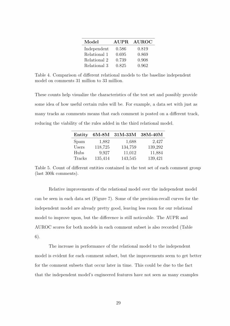
Model AUPR AUROC

Independent 0.586 0.819Relational 1 0.695 0.869Relational 2 0.739 0.908Relational 3 0.825 0.962

Table 4. Comparison of different relational models to the baseline independentmodel on comments 31 million to 33 million.

These counts help visualize the characteristics of the test set and possibly provide

some idea of how useful certain rules will be. For example, a data set with just as

many tracks as comments means that each comment is posted on a different track,

reducing the viability of the rules added in the third relational model.

Entity 6M-8M 31M-33M 38M-40M

Spam 1,882 1,688 2,427Users 118,725 134,759 139,292Hubs 9,927 11,012 11,884Tracks 135,414 143,545 139,421

Table 5. Count of different entities contained in the test set of each comment group(last 300k comments).

Relative improvements of the relational model over the independent model

can be seen in each data set (Figure 7). Some of the precision-recall curves for the

independent model are already pretty good, leaving less room for our relational

model to improve upon, but the difference is still noticeable. The AUPR and

AUROC scores for both models in each comment subset is also recorded (Table

6).

The increase in performance of the relational model to the independent

model is evident for each comment subset, but the improvements seem to get better

for the comment subsets that occur later in time. This could be due to the fact

that the independent model’s engineered features have not seen as many examples

29

— Independent - - - Relational

Figure 7. Relational model 3 tested on three different subsets of comments in thedata. Comments used: 6 million to 8 million, tested on the last 300k comments(left). Comments used: 31 million to 33 million, tested on the last 300k comments(Middle). Comments used: 38 million to 40 million, tested on the last 300kcomments (right).

Dataset AUPR (Ind) AUPR (Rel)

6M-8M 0.792 0.87331M-33M 0.588 0.82538M-40M 0.792 0.915

Table 6. Comparison of relational model 3 on different comment datasets.

for the earlier comments. This can cause less accurate predictions that get fed into

the relational model which might propagate information less accurately.

Extra Observations. One additional experiment used the previous

700K comments before the test set as extra evidence for the relational model.

Thus, more hubs, users, and tracks were inferred as spammy or non-spammy, and

this could help identify spam in the test set. For example, if a user shows up many

times posting spam in the evidence set, and only posts one comment in the test set,

it is easy to infer that the comment in the test set is probably also spam. Without

these extra observations, we have no previous evidence of what kind of user they

are, making it harder to classify their single comment in the test set.

30

After running relational model 3 with extra evidence on the 31 million to

33 million comment subset, the results did not make a big improvement over the

model without extra observations. This could be due to a lack of overlap between

users, matching comments, and tracks between the evidence and test sets, but this

lack of improvement is also encouraging. Since we already know that large increases

in performance can be made from doing joint inference over the test set, then we

know that we can get good results from a smaller graphical model that uses less

computation. So it is possible to reason that this evidence set can be replaced by a

larger test set where joint inference can label even more comments at the same time

with more accuracy than with a smaller test set. This implies the ability to scale

the relational model to label more instances collectively.

31

CHAPTER VI

CONCLUSION

From Jonathan Brophy and Daniel Lowd. 2017 AAAI Workshop on

Artificial Intelligence and Cyber-Security (AICS). San Francisco, CA.

We have shown the benefits of using a model that can leverage the

underlying connections present between the data in Soundcloud. With the aid of

an independent model to mark clear instances of spam and provide a starting point

of information, our relational model can work to identify the perhaps intentionally

obfuscated comments missed by the independent classifier.

We have seen that adding more rules to a relational classifier can increase its

performance, but adding too many can cause a bottleneck in computation time. It

is not hard to see the benefits of using a relational model, where implementations

like PSL make it very easy to express simple rules that can capture complex

relationships throughout the data.

One final aspect to note about this approach is the relationship between the

independent and relational models. Since the predictions from the independent

model are fed into the relational model, any performance improvement in the

independent model will most likely translate to improved performance for the

relational model as well. Thus, more in depth natural language processing (NLP)

features could be engineered for the independent model, but these are not explicitly

necessary to show the relative improvements of the relational model.

The next step of this work would involve testing this model on a different,

but similar domain to see if these results can be replicated. YouTube.com would

make an excellent choice, as its popularity certainly attracts many spammers, and

its social network structure is similar to that of SoundClouds’. Tracks could be

32

replaced by videos, since users post comments to other user’s videos the same way

users post comments to other user’s tracks. All the other rules can essentially stay

the same.

There is also the opportunity to learn weights in one domain, and then

test their effectiveness on another domain. Also, more work needs to be done on

characterizing the practical size of data instances that can be jointly labeled at

one time, and how this characterization changes as the number of rules increase or

decrease.

One segment of the data that was not used involved spam warnings and

spam reports. The ability of one user to flag other users is a common feature

in most social networks, and this information can lead to clues about who the

spammers are, as well as the credibility of users doing the flagging, as in Fakhraei

et al. (2015).

The applications for this kind of model are not bound to social networks.

Any type of data that houses underlying relations can benefit from this

methodology, and it is exciting to see what other domains relational machine

learning will impact.

33

REFERENCES CITED

Alvarez-Hamelin, J. I., Dall’Asta, L., Barrat, A., & Vespignani, A. (2005). Largescale networks fingerprinting and visualization using the k-coredecomposition. In Advances in neural information processing systems (pp.41–50).

Bach, S. H., Broecheler, M., Huang, B., & Getoor, L. (2015). Hinge-loss markovrandom fields and probabilistic soft logic. arXiv preprint arXiv:1505.04406 .

Bach, S. H., Huang, B., London, B., & Getoor, L. (2013). Hinge-loss Markovrandom fields: Convex inference for structured prediction. In Uncertainty inArtificial Intelligence (UAI).

Breiman, L. (2001). Random forests. Machine Learning , 45 , 5-32.

Davis, J., & Goadrich, M. (2006). The relationship between precision-recall and roccurves. In Proceedings of the 23rd international conference on machinelearning (pp. 233–240). New York, NY, USA: ACM. Retrieved fromhttp://doi.acm.org/10.1145/1143844.1143874 doi:10.1145/1143844.1143874

Fakhraei, S., Foulds, J., Shashanka, M., & Getoor, L. (2015). Collective spammerdetection in evolving multi-relational social networks. In Proceedings of the21th acm sigkdd international conference on knowledge discovery and datamining (pp. 1769–1778).

Kimmig, A., Bach, S. H., Broecheler, M., Huang, B., & Getoor, L. (2012). A shortintroduction to probabilistic soft logic. In NIPS Workshop on ProbabilisticProgramming: Foundations and Applications.

Laorden, C., Sanz, B., Santos, I., Galan-Garcıa, P., & Bringas, P. G. (2011).Collective classification for spam filtering. In A. Herrero & E. Corchado(Eds.), Computational intelligence in security for information systems: 4thinternational conference, cisis 2011, held at iwann 2011,torremolinos-malaga, spain, june 8-10, 2011. proceedings (pp. 1–8). Berlin,Heidelberg: Springer Berlin Heidelberg. Retrieved fromhttp://dx.doi.org/10.1007/978-3-642-21323-6 1 doi:10.1007/978-3-642-21323-6 1

Lee, K., Caverlee, J., Kamath, K. Y., & Cheng, Z. (2012). Detecting collectiveattention spam. In Proceedings of the 2nd joint wicow/airweb workshop onweb quality (pp. 48–55).

34

Liu, L., Lu, Y., Luo, Y., Zhang, R., Itti, L., & Lu, J. (2016). Detecting” smart”spammers on social network: A topic model approach. arXiv preprintarXiv:1604.08504 .

LOGIC, L., Garrido, A., & Garrido, A. (2010). Fuzzy boolean algebras andlukasiewicz logic..

Low, Y., Gonzalez, J., Kyrola, A., Bickson, D., Guestrin, C., & Hellerstein, J. M.(2010). Graphlab: A new framework for parallel machine learning. In Uai.

Newman, M. E., Strogatz, S. H., & Watts, D. J. (2001). Random graphs witharbitrary degree distributions and their applications. Physical review E ,64 (2), 026118.

Page, L., Brin, S., Motwani, R., & Winograd, T. (1999). The pagerank citationranking: bringing order to the web.

Pearl, J. (2014). Probabilistic reasoning in intelligent systems: networks of plausibleinference. Morgan Kaufmann.

Pedregosa, F., Varoquaux, G., Gramfort, A., Michel, V., Thirion, B., Grisel, O., . . .Duchesnay, E. (2011). Scikit-learn: Machine learning in python. Journal ofMachine Learning Research, 12 , 2825-2830.

Quinlan, J. R. (1986). Induction of decision trees. Machine Learning , 1 , 81-106.

Rayana, S., & Akoglu, L. (2015). Collective opinion spam detection: Bridgingreview networks and metadata. In Proceedings of the 21th acm sigkddinternational conference on knowledge discovery and data mining (pp.985–994).

Richardson, M., & Domingos, P. M. (2006). Markov logic networks. MachineLearning , 62 , 107-136.

Schank, T., & Wagner, D. (2005). Finding, counting and listing all triangles inlarge graphs, an experimental study. In International workshop onexperimental and efficient algorithms (pp. 606–609).

Sen, P., Namata, G., Bilgic, M., Getoor, L., Galligher, B., & Eliassi-Rad, T. (2008).Collective classification in network data. AI magazine, 29 (3), 93.

Wang, D., & Pu, C. (2015, Aug). Bean: A behavior analysis approach of url spamfiltering in twitter. In 2015 ieee international conference on informationreuse and integration (p. 403-410). doi: 10.1109/IRI.2015.69

Zadeh, L. A. (1988). Fuzzy logic. Computer , 21 , 83-93.

35

Zhu, Y., Wang, X., Zhong, E., Liu, N. N., Li, H., & Yang, Q. (2012). Discoveringspammers in social networks. In Aaai.

36