Collapse of charged scalar field in dilaton gravity

Anna Borkowska* and Marek Rogatko†

Institute of Physics, Maria Curie-Sklodowska University, 20-031 Lublin, pl. Marii Curie-Sklodowskiej 1, Poland

Rafał Moderski‡

Nicolaus Copernicus Astronomical Center, Polish Academy of Sciences, 00-716 Warsaw, Bartycka 18, Poland(Received 21 January 2011; published 6 April 2011)

We elaborated the gravitational collapse of a self-gravitating complex charged scalar field in the context

of the low-energy limit of the string theory, the so-called dilaton gravity. We begin with the regular

spacetime and follow the evolution through the formation of an apparent horizon and the final central

singularity.

DOI: 10.1103/PhysRevD.83.084007 PACS numbers: 04.25.dg, 04.40.�b

I. INTRODUCTION

The long-standing prediction of general relativity is theoccurrence of spacetime singularity inside black holes. Thesingularity theorems of Penrose and Hawking [1] predictthe occurrence of spacetime singularities inside black holesunder very plausible assumptions, but tell nothing aboutthe geometrical and physical nature and properties of theemerging singularities.

Until recently the only known generic singularitywas the Belinsky-Khalatnikov-Lifshitz (BKL) one [2].According to this picture spacetime develops a successionof Kasner epochs in which the axes of contraction andexpansion change chaotically. This singularity has a strongoscillatory character, which is highly destructive for anyphysical object. Soon after Belinsky et al. [3] used a scalarfield to have an insight into a cosmological singularityproblem of BKL. They found that scalar fields destroyedBKL oscillations and singularity became monotonic.Recently, it was shown [4] that the general solutions nearspacelike singularity in superstring theories and inM-theory (the Einstein-dilaton-p-form field) exhibit anoscillatory character of BKL type.

For a Schwarzschild black hole it has been shown thatthe asymptotic portion of spacetime near singularity is freeof aspherical perturbations propagated from the star’s sur-face since the gravitational radiation is infinitely diluted asit reaches the singularity. On the other hand, the internalstructure of the Reissner-Nordstrom (RN) or Kerr blackhole differs significantly from the above picture. The sin-gularity becomes timelike and both of these spacetimespossess Cauchy horizons (null hypersurfaces beyondwhich predictability breaks down). In the last few years anew picture of the inner structure of black holes wasachieved, according to which the Cauchy horizon inside

the RN or Kerr black hole transforms into a null, weaksingularity, i.e., an infalling observer hitting this null sin-gularity experiences only a finite tidal deformation [5,6].The curvature scalars and mass parameter diverge alongthis Cauchy singularity and this phenomenon is known asmass-inflation. The physical mechanism on which theCauchy horizon singularity is based is strictly connectedwith small perturbations (remnants of gravitational col-lapse) which are gravitationally blue-shifted as they propa-gate in the black hole interior parallel to the Cauchyhorizon. For a toy model of the spherically symmetriccharged black hole the main features of singularity at theinner horizon were first deduced analytically from simpli-fied examples based on null fluids [7,8].Most of the conclusions supporting the existence of a

null weak Cauchy horizon singularity were obtained bymeans of a perturbative analysis. The full nonlinear inves-tigations of the inner structure of black holes were given inRef. [9] where the authors revealed that a central spacelikesingularity is located deep inside a charged black holecoupled to a neutral scalar field. The existence of a nullmass-inflation singularity was established by Brady andSmith [6], in their studies of nonlinear evolution of aneutral scalar field on a spherical charged black hole.Burko [10] also studied the same problem and found avery good agreement between the nonlinear numericalanalysis and the predictions of the perturbative analysis.Expressions for the divergence rate of the blue-shiftedfactors for that model valid everywhere along Cauchyhorizon, were given analytically in Ref. [11]. One shouldhave in mind that all these numerical works were begin-ning on RN spacetime and a black hole formation was notcalculated. Numerical studies of the spherically symmetriccollapse of a massless scalar field in the semiclassicalapproximation were conducted in Ref. [12]. Piran et al.[13] studied the inner structure of a charged blackhole formed during the gravitational collapse of a self-gravitating charged scalar field. They started with a regularspacetime and conducted the evolution through the

*aborkow@kft.umcs.lublin.pl†rogat@kft.umcs.lublin.pl;

marek.rogatko@poczta.umcs.lublin.pl‡moderski@camk.edu.pl

PHYSICAL REVIEW D 83, 084007 (2011)

1550-7998=2011=83(8)=084007(21) 084007-1 � 2011 American Physical Society

formation of an apparent horizon, Cauchy horizon anda final singularity. The results obtained in [13] were con-firmed and refined in Refs. [14,15].

The effect of pair creation in the strong electric fields ina dynamical model of a collapse of the self-gravitatingelectrically charged massless scalar field was elaboratedin [16]. The authors studied the discharge below the eventhorizon and its influence on the dynamical formation of theCauchy horizon. On the other hand, the dynamical forma-tion and evaporation of a spherically charged black holesupposed initially to be nonextremal but tending towardsthe extremal black hole and moreover emitting Hawkingradiation was investigated in Ref. [17]. Recently, a spheri-cally symmetric charged black hole with a complex scalarfield, gauge field and renormalized energy-momentumtensor (in order to take into account the Hawking radiation)was considered in [18]. When the Hawking radiation wasincluded it turned out that the inner horizon was separatedfrom the Cauchy one. Studying the neutralization of thecharged black hole in question it was found that the innerhorizon evolved into a spacelike singularity. Using theexponentially large number of scalar particles it happenedthat one could extend investigations inside the inner hori-zon. Recently, the response of the Brans-Dicke field duringgravitational collapse of matter was analyzed [19] whilethe internal structure of charged black hole includingHawking radiation and discharge was elaborated in [20].In Ref. [21] the first axisymmetric numerical code testingthe gravitational collapse of a complex scalar field waspresented. Also the nonlinear processes with the participa-tion of an exotic scalar field modeled as a free scalar fieldwith an opposite sign in the energy-momentum tensor wereconsidered [22] due to the case when the RN black holewas irradiated by this kind of matter.

In this paper we shall consider the implication of super-string gravity for the dynamical collapse of the chargedcomplex scalar field. The famous Wheeler’s dictum thatblack holes have no hair predicts that the inner structure ofthe black hole will not depend on the collapsing fields. Inmathematical formulation this conjecture corresponds tothe so-called black hole uniqueness theorem [23] (classifi-cation of the domains of outer communication of regularblack hole spacetimes). On the other hand, various aspectsof the uniqueness theorem for four-dimensional blackholes in the low-energy string theory were widely treatedin Refs. [24].

In previous papers [25] we have examined the inter-mediate and late-time behavior of matter fields (scalarand fermions) in the background of dilaton black holes.In some way the present studies will generalize the formerones to the more realistic toy model of the dynamicalcollapse. In what follows we assume that the consideredLagrangian for the charged complex scalar field will becoupled to the dilaton via an arbitrary coupling, i.e.,e2��Lðc ; c �; AÞ, in the string frame. The outline of the

remainder of the paper is as follows. In Sec. II we derivethe equations describing the collapse of the charged scalarfield in the presence of nontrivial coupling to the dilatonfield. Section III was devoted to the numerical schemeapplied in our investigations. We discussed the numericalalgorithm, an adaptive grid used in computations, and theboundary and initial conditions for the equations of motionfor the considered problem. We also paid attention to theaccuracy of our numerical code. Section IV is assigned tothe discussion of the obtained results. In Sec. V we con-cluded our researche.

II. DILATON BLACK HOLE

In this section our main interests will concentrate on thebehavior of the collapsing complex charged scalar fieldwhen gravitational interactions take a form typical for thelow-energy string theory, the so-called dilaton gravity. Totake into account the unknown coupling of the dilaton fieldto the considered charged complex scalar field, we choosethe action in the form

I ¼Z

d4xffiffiffiffiffiffiffi�g

p ½e�2�ðR� 2ðr�Þ2 þ e2��LÞ�; (1)

where the Lagrangian L is given by

L ¼ � 1

2ðr�c þ ieA�c Þg��ðr�c

� � ieA�c�Þ

� F��F��: (2)

The action is written in the string frame but it will be usefulto rewrite it in the Einstein frame. In the Einstein frame themetric is related to the string frame via the conformaltransformation of the form provided by the following:

g�� ¼ e�2�g��: (3)

The gravitational part of the action (1) appears in theEinstein frame in a more familiar form. Namely, it impliesthe following:

I ¼Z

d4xffiffiffiffiffiffiffi�g

p ½R� 2ðr�Þ2

þ e2��þ4�Lðc ; c �; A; e2�g��Þ�: (4)

The equations of motion derived from the variational prin-ciple yield

r2���þ1

4e2�ð�þ1Þðr�c þ ieA�c Þ

�ðr�c �� ieA�c �Þ�1

2�e2��F2¼0; (5)

r�ðe2��F��Þ þ e2�ð�þ1Þ

4½iec �ðr�c þ ieA�c Þ

� iec ðr�c � � ieA�c �Þ� ¼ 0; (6)

ANNA BORKOWSKA, MAREK ROGATKO, AND RAFAŁ MODERSKI PHYSICAL REVIEW D 83, 084007 (2011)

084007-2

r2c þ ieA�ð2r�c þ ieA�c Þ þ ier�A�c ¼ 0; (7)

r2c � � ieA�ð2r�c� � ieA�c

�Þ � ier�A�c � ¼ 0;

(8)

G�� ¼ T��ð�;F; c ; c �; AÞ; (9)

where the energy-momentum tensor T��ð�;F; c ; c �; AÞfor the fields in the theory under consideration is providedby the relation

T��ð�;F; c ; c �; AÞ ¼ e2�ð�þ1Þ ~T��ðc ; c �; AÞþ T��ðF;�Þ: (10)

In Eq. (10) by ~T��ðc ; c �; AÞ we have denoted the follow-

ing expression:

~T��ðc ; c �; AÞ ¼ 1

4½iec ðA�r�c

� þ A�r�c�Þ

� iec �ðA�r�c þ A�r�c Þ�þ 1

4ðr�cr�c

� þ r�c�r�c Þ

þ 1

2e2A�A�c c � þ 1

2~Lðc ; c �; AÞg��;

(11)

where the explicit form of the Lagrangian ~Lðc ; c �; AÞ iswritten as

~Lðc ; c �; AÞ ¼ � 1

2ðr�c þ ieA�c Þðr�c � � ieA�c �Þ:

(12)

On the other hand, for T��ðF;�Þ one gets

T��ðF;�Þ ¼ e2���2F��F�

� � 1

2g��F

2

�� g��ðr�Þ2

þ 2r��r��: (13)

In order to study the gravitational collapse in a sphericallysymmetric spacetime it will be useful to consider the lineelement written in the double-null form [26]

ds2 ¼ �aðu; vÞ2dudvþ r2ðu; vÞd�2; (14)

where u, v are advanced and retarded time null coordi-nates. The null character of the coordinates in question willbe preserved by the gauge transformation of the form u !fðuÞ and v ! gðvÞ. Using doubly null coordinates enablesus to begin with the regular initial spacetime at approxi-mately past null infinity, compute the formation of blackhole’s event horizon and then prolong the evolution of theblack hole to the central singularity formed during thedynamical collapse. The assumption of spherical symme-try and the above coordinate choice imply that the onlynonvanishing component of the Uð1Þ-gauge strength fieldis Fuv or Fvu. Consequently, it provides another restriction

on the gauge potential. Namely, one has to do with Au orAv. We can get rid of one of these components of gaugepotential by using the gauge freedom of the form Au !Au þru�. If one chooses � ¼ R

Avdv, then we are left

with the only one component of the gauge field, which isthe function of u and v-coordinates.To proceed further, we take into account the

v-component of the generalized Einstein-Maxwell equa-tions. It leads to the following relation:

�2e2��r2Au;v

a2

�;vþ r2e2�ð�þ1Þ

4ieðc �c ;v � c c �

;vÞ ¼ 0:

(15)

Let us define the quantity

Q ¼ 2Au;vr

2

a2; (16)

just as in Ref. [14]. Q corresponds to the electric chargewithin the sphere of the radius rðu; vÞ. The above definitionenables us to separate the second-order partial differentialequation for Au into two much simpler first-order differ-ential equations. We arrive at the following:

Au;v �Qa2

2r2¼ 0; (17)

and

Q;v þ 2��;vQþ ier2

4e2�ðc �c ;v � c c �

;vÞ ¼ 0: (18)

The equation of motion for dilaton field (5) has the formprovided by

r;u�;v þ r;v�;u þ r�;uv � ð�þ 1Þ8

e2�ð�þ1Þ

� r½c ;uc�;v þ c ;vc

�;u þ ieAuðc c �

;v � c �c ;v�

� �a2Q2e2��

4r3¼ 0: (19)

Consequently, the relations for the complex scalar fieldsare given by

r;uc ;v þ r;vc ;u þ rc ;uv þ ierAuc ;v þ ier;vAuc

þ ieQa2

4rc ¼ 0; (20)

r;uc�;v þ r;vc

�;u þ rc �

;uv � ierAuc�;v � ier;vAuc

�

� ieQa2

4rc � ¼ 0: (21)

Combining the adequate components of the Einstein tensorand the stress-energy tensor for the underlying theory weobtain the following set of equations:

COLLAPSE OF CHARGED SCALAR FIELD IN DILATON . . . PHYSICAL REVIEW D 83, 084007 (2011)

084007-3

2a;ur;ua

�r;uu¼ r�2;uþre2�ð�þ1Þ

4½c ;uc

�;uþ ieAu

�ðc c �;u�c �c ;uÞþe2A2

uc c ��; (22)

2a;vr;va

� r;vv ¼ r�v2 þ 1

4re2�ð�þ1Þc ;vc

�;v; (23)

a2

4rþ r;urv

rþ r;uv ¼ e2��a2Q2

4r3; (24)

a;ua;va2

�a;uva

�r;uvr

¼Q2e2��a2

4r4þ�;u�;vþe2�ð�þ1Þ

8

�½c ;uc�;vþc �

;uc ;vþ ieAuðc c �v�c �c ;vÞ�: (25)

Moreover, we introduce new auxiliary variables written inthe form as

c ¼ a;ua

; d ¼ a;va

; f ¼ r;u; g ¼ r;v;

s ¼ c ; p ¼ c ;u; q ¼ c ;v; � ¼ Au;

k ¼ �; x ¼ �;u; y ¼ �;v;

(26)

and the additional quantities provided by the relations asfollows:

� a2

4þ fg; (27)

� � fqþ gp; (28)

� gxþ fy: (29)

Instead of considering two complex fields c and c � onecan introduce two real fields obeying the relations c ¼c 1 þ ic 2 and c

� ¼ c 1 � ic 2. On this account, it leads to

s ¼ s1 þ is2; p ¼ p1 þ ip2; q ¼ q1 þ iq2;

(30)

� ¼ �1 þ i�2;

�1 ¼ fq1 þ gp1;

�2 ¼ fq2 þ gp2:

(31)

Thus, having in mind all the above, one can rewrite thesystem of the second-order partial differential equations asthe first-order one. By this procedure we get the followingsystem of the first-order differential equations:

P1: a;u � ac ¼ 0; (32)

P2: a;v � ad ¼ 0; (33)

P3: r;u � f ¼ 0; (34)

P4: r;v � g ¼ 0; (35)

P5ðReÞ: s1;u � p1 ¼ 0; (36)

P5ðImÞ: s2;u � p2 ¼ 0; (37)

P6ðReÞ: s1;v � q1 ¼ 0; (38)

P6ðImÞ: s2;v � q2 ¼ 0; (39)

P7: k;u � x ¼ 0; (40)

P8: k;v � y ¼ 0; (41)

E1: f;u�2cfþrx2þ1

4re2kð�þ1Þ½p2

1þp22

þ2e�ðs1p2�s2p1Þþe2�2ðs21þs22Þ�¼0; (42)

E2:g;v�2dgþry2þ1

4re2kð�þ1Þðq21þq22Þ¼0; (43)

E3ð1Þ: f;v þ

r� e2�k

Q2a2

4r3¼ 0; (44)

E3ð2Þ: g;u þ

r� e2�k

Q2a2

4r3¼ 0; (45)

E4ð1Þ: c;v �

r2þ xyþ 1

4e2kð�þ1Þ½p1q1 þ p2q2

þ e�ðs1q2 � s2q1Þ� þ e2�kQ2a2

2r4¼ 0; (46)

E4ð2Þ: d;u�

r2þxyþ1

4e2kð�þ1Þ

�½p1q1þp2q2þe�ðs1q2�s2q1Þ�þe2�kQ2a2

2r4¼0;

(47)

Sð1ÞðReÞ: rp1;v þ�1 � er�q2 � es2�g� es2Qa2

4r¼ 0;

(48)

Sð1ÞðImÞ: rp2;v þ�2 þ er�q1 þ es1�gþ es1Qa2

4r¼ 0;

(49)

Sð2ÞðReÞ: rq1;u þ�1 � er�q2 � es2�g� es2Qa2

4r¼ 0;

(50)

ANNA BORKOWSKA, MAREK ROGATKO, AND RAFAŁ MODERSKI PHYSICAL REVIEW D 83, 084007 (2011)

084007-4

Sð2ÞðImÞ: rq2;u þ�2 þ er�q1 þ es1�gþ es1Qa2

4r¼ 0;

(51)

Dð1Þ: rx;v þ � �þ 1

4re2kð�þ1Þ½p1q1 þ p2q2

þ e�ðs1q2 � s2q1Þ� � �e2�kQ2a2

4r3¼ 0; (52)

Dð2Þ: ry;u þ � �þ 1

4re2kð�þ1Þ½p1q1 þ p2q2

þ e�ðs1q2 � s2q1Þ� � �e2�kQ2a2

4r3¼ 0; (53)

M1: �;v �Qa2

2r2¼ 0; (54)

M2: Q;v þ 2�yQ� 1

2e2ker2ðs1q2 � s2q1Þ ¼ 0: (55)

Let us introduce some quantities of physical interest.Namely, we define the mass function provided by therelation

mðu; vÞ ¼ r

2

�1þ 4r;ur;v

a2

�¼ r

2

�1þ 4

a2fg

�: (56)

It represents the Hawking mass, i.e., the mass included in asphere of the radius rðu; vÞ. Moreover, the Ricci scalar hasthe form as

Rðu; vÞ ¼ � 16xy

a2� 2

a2e2kð�þ1Þ½pq� þ qp�

þ ie�ðsq� � qs�Þ�; (57)

or it can be rewritten in the form which yields thefollowing:

Rðu; vÞ ¼ � 16xy

a2� 4

a2e2kð�þ1Þ½p1q1 þ p2q2

þ e�ðs1q2 � s2q1Þ�: (58)

III. NUMERICAL COMPUTATIONS

A. Numerical algorithm

The system of Eqs. (32)–(55) in the theory under con-sideration has to be solved numerically. In order to find thesolution one should elaborate an evolution of the quantitiesd, q1, q2, y, a, s1, s2, k, g, r, Q, �, f, p1, p2 and x. Thequantity c does not play the significant role in the processunder consideration, so it can be ignored. The evolution ofthe quantities d, q1, q2 and y along u is governed by

relations E4ð2Þ, Sð2ÞðReÞ, Sð2ÞðImÞ and Dð2Þ, respectively. The

remaining quantities, a, s1, s2, k, g, r, Q, �, f, p1, p2

and x evolve in turn along the v-coordinate according to

equations P2, P6ðReÞ, P6ðImÞ, P8, E2, P4, M2, M1, E3ð1Þ,

Sð1ÞðReÞ, Sð1ÞðImÞ and Dð1Þ. On the other hand, Eqs. P1 and E4ð1Þ

describing the behavior of c may be discarded and theremaining relations can be used to determine the boundaryconditions.In our studies the numerical algorithm similar to the one

proposed in [27] was implemented. The computations werecarried out on the two-dimensional grid constructed in theðvuÞ-plane. In order to obtain a value of a particularfunction at a point ðv; uÞ one should have values of theappropriate functions at points ðv� hv; uÞ and ðv; u� huÞ,where hv and hu are integration steps in v and u directions,respectively. Equations describing the evolution of theconsidered quantities along the coordinates u and v maybe symbolically written as:

f;u ¼ Fðf; gÞ; g;v ¼ Gðf; gÞ: (59)

In order to get the value of the particular function at apoint ðv; uÞ, we should find the auxiliary quantities whichyield

f fjðv;uÞ ¼ fjðv;u�huÞ þ huFðf; gÞjðv;u�huÞ; (60)

g gjðv;uÞ ¼ gjðv�hv;uÞ þhv2ðGðf; gÞjðv;uÞ þGðff; ggÞjðv;uÞÞ:

(61)

By virtue of the above the final values of the quantities inquestion are provided by the following:

f jðv;uÞ ¼ 1

2ðffjðv;uÞ þ fjðv;u�huÞ þ huFðff;ggÞjðv;uÞÞ; (62)

g jðv;uÞ ¼ 1

2ðggjðv;uÞ þ gjðv�hv;uÞ þ hvGðff; ggÞjðv;uÞÞ:

(63)

In the early stages of the calculations the numerical grid isdivided evenly, both in v and u directions. On this account,at the beginning the quantities hv and hu are equal to eachother.

B. Adaptive mesh refinement

The coordinates u and v ensure the regular behavior ofall the considered quantities within the domain of integra-tion except the vicinity of r ¼ 0. However, during thenumerical analysis the considerable difficulties also ariseclose to the event horizon, where function f diverges. Arelatively dense numerical grid is necessary in order tosatisfactorily determine the location of the event horizonand to examine the behavior of fields inside it, especiallyfor large values of the v-coordinate. The efficiency of thecalculations suggests using an adaptive grid and perform-ing integration with a smaller step, in particular, regions.On this account the refinement algorithms enable us tomake the grid denser both in v and u directions and todo the same only along u-coordinate. The first one makes

COLLAPSE OF CHARGED SCALAR FIELD IN DILATON . . . PHYSICAL REVIEW D 83, 084007 (2011)

084007-5

the integration steps hv and hu smaller on the equal footingas one approaches the event horizon and reaches the largevalues of v. The other one changes only the value of hu. Itturned out that the latter refinement of the adaptive gridgives the satisfactory results and it is more effective due tothe computation time and required computer’s memory.Hence, all the results presented in our paper will be basedon it.

In order to determine the area of the integration grid,where the grid should be denser, a local error indicatorneed to be used. The aforementioned quantity ought to bebounded with the evolving quantities as well as it shouldchange its value significantly in the adequate region. Ithappened that [14] the function �r=r along u-coordinatemeets our requirements.

C. Boundary and initial conditions

Having specified the numerical algorithm for the solu-tion of the equations of motion we refine our studies to thecase of the initial and boundary conditions for the equa-tions in question. The boundary conditions refer to thesurface u ¼ v, while the initial conditions are formulatedalong an arbitrarily chosen constant surface u ¼ ui. Apoint (0, 0) is chosen to be the intersection of these twolines in the ðvuÞ-plane. It also indicates the center of theconsidered spacetime.

The physical situation we shall take into account will bethe gravitational collapse of a spherically symmetric shellof infalling complex charged matter. The spacetime of aspherical shell of matter is flat in two regions, i.e., insidethe shell and at large radii from it. This fact enables us toassume that the line u ¼ vwill be not significantly affectedby the presence of the collapsing shell of matter. On thisaccount the spacetime may be considered as nearly flat andelectrically neutral in that region. Thus, it gives the follow-ing boundary conditions: r ¼ Q ¼ � ¼ 0. Consequently,

equations E3ð1;2Þ reveal that ¼ 0 along u ¼ v. This facttogether with Eqs.P3 and P4 provides that f ¼ �g ¼ � a

2 .

Furthermore, the requirement s1;r ¼ s2;r ¼ k;r ¼ a;r ¼ 0along u ¼ v guarantees that the field functions flatten nearr ¼ 0 making the numerical analysis possible. Because ofthe fact that r changes nonlinearly along the coordinates uand v this boundary condition is implemented using thethree-point regressive derivative method with a variablestep, except the first point, where the Euler’s method isused.

Combining the relation �1 ¼ �2 ¼ ¼ 0 along the

u ¼ v line and Eqs. Sð1;2ÞðReÞ , we obtain that p1 ¼ q1,

p2 ¼ q2 and x ¼ y. On the other hand, the boundary con-ditions for the quantities evolving along u can be achievedaccording to the algorithm described in the previous sec-tion. It can be seen that the auxiliary quantities (61) aretaken to be equal to the corresponding functions at r ¼ 0.

The assumption of the flat geometry in the region,where an observation of the collapse begins, justifies the

condition that dðv; 0Þ ¼ 0. Further, it fixes the remainingfreedom in the v-coordinate. By virtue of the flatness of thespacetime in the vicinity of a surface u ¼ v and the aboveassumptions we get that aðv; 0Þ ¼ 1. One should mentionthat the initial conditions ought to include the arbitraryprofiles for scalar functions s1ðv; 0Þ and s2ðv; 0Þ describingthe real and the imaginary parts of the charged scalar fieldand for the dilaton field kðv; 0Þ. The one-parameter fami-lies of the initial profiles are listed in Table I, where a freefamily parameter is denoted as ~p, constants c1 and c2 arearbitrarily chosen, while vf equals the final value of v. � 2½0; �2� is a phase difference determining the amount of the

initial electric charge [20]. The quantities q1ðv; 0Þ,q2ðv; 0Þ, and yðv; 0Þ are computed analytically using equa-tions P6ðReÞ, P6ðImÞ, and P8. The values of the functions g,r, Q, �, f, p1, p2, and x along the axis u ¼ 0 are obtainedusing the three-point Simpson’s method apart from the firstpoint, where the Newton’s method is implemented.

D. Numerical tests

The most straightforward manner of checking the cor-rectness of the numerical code will be a comparison be-tween achieved results and an analytical solution of theconsidered problem. Unfortunately, because of the lack ofthe analytical solution of the problem in question oneshould apply indirect methods of checking the accuracyof the numerical code.The first trial will be checking of the convergence of the

obtained results. One verifies that the fields under consid-eration converge to some values in the expected region ofconvergence. From the numerical point of view it envi-sages the fact that the algorithm and its implementation arefree of mistakes. To begin with we carried the computa-tions not requiring adaptive mesh on four different gridswith integration steps equal in both directions. The inte-gration step of the particular grid was twice the size of adenser one. The evolving field profiles for arbitrarilychosen u-coordinate are shown in Fig. 1. We scaled upthe vicinities of the cusps, where the differences amongprofiles were most significant. For all the field profiles thevery good agreement of an order of 0.01% was achieved.On the other hand, the linear convergence of the numericalcode is presented in Fig. 2. The differences between theprofiles obtained on the two grids with a quotient of theintegration steps equal to 2 and their respective doubles arehardly distinguishable. The divergence is at most 1%, asmay be inferred from the values shown in the magnified

TABLE I. Initial profiles of field functions.

Family Profile

ðfDþSÞ ~p � v2 � e�ðv�c1=c2Þ2

ðfSÞ ~p � sin2ð� vvfÞ � ðcosð� 2v

vfÞ þ i cosð� 2v

vfþ �ÞÞ

ANNA BORKOWSKA, MAREK ROGATKO, AND RAFAŁ MODERSKI PHYSICAL REVIEW D 83, 084007 (2011)

084007-6

areas. Moreover, Fig. 2 gives clear evidence that the errorsbecome smaller as the grid density increases.The next test of our code is to check whether mass (56)

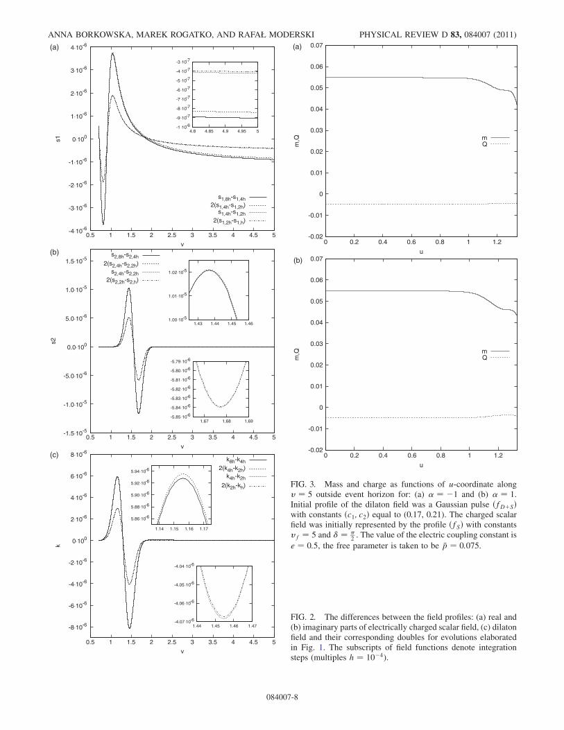
and charge (16) are conserved in the evolving spacetime.The considered fields are scattered by the gravitational andelectromagnetic potential barriers as the collapsing shellapproaches its gravitational radius. Therefore the conser-vation laws are not satisfied in the entire domain of inte-gration. Nevertheless, this effect of the outgoing fluxes ofmass and charge is negligible [14] and it has no significantinfluence on the total mass and charge, excluding the areain the vicinity of the new forming black hole event horizon.In Fig. 3 the behaviors of mass and charge for the largevalue of the advanced time are presented. It turned out thatfor u not exceeding 1, mass and charge are conserved up towithin 1.6% and 2.5%, respectively. Further, the inspectionof Fig. 3 reveals the deviation of the aforementionedquantities from constancy increases with the advancedtime. It is caused due to the fact that the reflected wavescarry off some mass as well as charge. Because of the factthat the total mass contains also the energy-momentum ofthe gravitational field, which is not taken into accountin the Noether current bounded with the energy-momentum tensor, the subject of the mass conservationis more subtle [14].The last test of the accuracy of our code consists of the

analysis of the simplified versions of the problem in ques-tion. Namely, in Fig. 4 we depicted the outgoing nullrays in ðrvÞ-plane for the spacetime containing theblack hole stemmed from the gravitational collapse of theneutral scalar field. The situation corresponds to setting� ¼ e ¼ 0 in the equations of motion and eliminating theelectrically charged scalar field by putting c ¼ 0. Thevalue of the free parameter is equal to 0.125. On the otherhand, Fig. 5 illustrates the outgoing null rays for the space-time of a black hole emerging due to the gravitationalcollapse of an electrically charged scalar fields. Here, weput � ¼ 0 and get rid of the dilaton field by setting � ¼ 0.The value of the free parameter was taken to be 0.5. Theinspection of Fig. 5 shows the formation of the black holeevent horizon and a Cauchy horizon at asymptotically largev. The structures of the spacetimes emerging during col-lapses presented in Figs. 4 and 5 are in a perfect agreementwith the results published in Refs. [13,14,27].

-0.006

-0.004

-0.002

0

0.002

0.004

0.006

0.008

0.01

0.012

0.014

0.5 1 1.5 2 2.5 3 3.5 4 4.5 5

s1

v

(a)h

2h4h8h

-0.00415

-0.00414

-0.00413

-0.00412

-0.00411

-0.0041

1 1.01 1.02 1.03 1.04 1.05

-0.005

0

0.005

0.01

0.015

0.02

0.025

0.5 1 1.5 2 2.5 3 3.5 4 4.5 5

s2

v

(b)h

2h4h8h

0.02195

0.02196

0.02197

0.02198

0.02199

0.022

0.02201

1.55 1.555 1.56 1.565 1.57

0

0.005

0.01

0.015

0.02

0.5 1 1.5 2 2.5 3 3.5 4 4.5 5

k

v

(c)h

2h4h8h

0.01834

0.01835

0.01836

0.01837

0.01838

0.01839

0.0184

1.3 1.31 1.32 1.33 FIG. 1. Plots of the field profiles: (a) real and (b) imaginaryparts of electrically charged scalar field, (c) dilaton field, alongu ¼ 0:7 taken for the different integration steps (multiples ofh ¼ 10�4). The evolution was monitored for a Gaussian initialpulse ðfDþSÞ with the parameter ~p ¼ 0:005 and constantsðc1; c2Þ equal to (0.75, 0.15), (1.55, 0.17), (1.3, 0.21), respec-tively. The values of the coupling constants are � ¼ 1 ande ¼ 0:5.

COLLAPSE OF CHARGED SCALAR FIELD IN DILATON . . . PHYSICAL REVIEW D 83, 084007 (2011)

084007-7

-4⋅10-6

-3⋅10-6

-2⋅10-6

-1⋅10-6

0⋅100

1⋅10-6

2⋅10-6

3⋅10-6

4⋅10-6

0.5 1 1.5 2 2.5 3 3.5 4 4.5 5

s1

v

(a)

s1,8h-s1,4h2(s1,4h-s1,2h)

s1,4h-s1,2h2(s1,2h-s1,h)

-1 ⋅10-6

-9 ⋅10-7

-8 ⋅10-7

-7 ⋅10-7

-6 ⋅10-7

-5 ⋅10-7

-4 ⋅10-7

-3 ⋅10-7

4.8 4.85 4.9 4.95 5

-1.5⋅10-5

-1.0⋅10-5

-5.0⋅10-6

0.0⋅100

5.0⋅10-6

1.0⋅10-5

1.5⋅10-5

0.5 1 1.5 2 2.5 3 3.5 4 4.5 5

s2

v

(b) s2,8h-s2,4h

2(s2,4h-s2,2h)s2,4h-s2,2h

2(s2,2h-s2,h)

1.00 ⋅10-5

1.01 ⋅10-5

1.02 ⋅10-5

1.43 1.44 1.45 1.46

-5.85 ⋅10-6

-5.84 ⋅10-6

-5.83 ⋅10-6

-5.82 ⋅10-6

-5.81 ⋅10-6

-5.80 ⋅10-6

-5.79 ⋅10-6

1.67 1.68 1.69

-8⋅10-6

-6⋅10-6

-4⋅10-6

-2⋅10-6

0⋅100

2⋅10-6

4⋅10-6

6⋅10-6

8⋅10-6

0.5 1 1.5 2 2.5 3 3.5 4 4.5 5

k

v

(c)k8h-k4h

2(k4h-k2h)k4h-k2h

2(k2h-kh)

5.86 ⋅10-6

5.88 ⋅10-6

5.90 ⋅10-6

5.92 ⋅10-6

5.94 ⋅10-6

1.14 1.15 1.16 1.17

-4.07⋅10-6

-4.06 ⋅10-6

-4.05 ⋅10-6

-4.04 ⋅10-6

1.44 1.45 1.46 1.47

FIG. 2. The differences between the field profiles: (a) real and(b) imaginary parts of electrically charged scalar field, (c) dilatonfield and their corresponding doubles for evolutions elaboratedin Fig. 1. The subscripts of field functions denote integrationsteps (multiples h ¼ 10�4).

-0.02

-0.01

0

0.01

0.02

0.03

0.04

0.05

0.06

0.07

0 0.2 0.4 0.6 0.8 1 1.2

m,Q

u

(a)

mQ

-0.02

-0.01

0

0.01

0.02

0.03

0.04

0.05

0.06

0.07

0 0.2 0.4 0.6 0.8 1 1.2

m,Q

u

(b)

mQ

FIG. 3. Mass and charge as functions of u-coordinate alongv ¼ 5 outside event horizon for: (a) � ¼ �1 and (b) � ¼ 1.Initial profile of the dilaton field was a Gaussian pulse ðfDþSÞwith constants ðc1; c2Þ equal to (0.17, 0.21). The charged scalarfield was initially represented by the profile ðfSÞ with constantsvf ¼ 5 and � ¼ �

2 . The value of the electric coupling constant is

e ¼ 0:5, the free parameter is taken to be ~p ¼ 0:075.

ANNA BORKOWSKA, MAREK ROGATKO, AND RAFAŁ MODERSKI PHYSICAL REVIEW D 83, 084007 (2011)

084007-8

IV. RESULTS

In our numerical studies we have used the one-parameterfamilies of initial profiles referring to the real and imagi-nary parts of the electrically charged scalar field anddilaton field. The results do not depend on the type of thefamily of the initial profiles as well as on family constants.Hence their choice is unrestricted. Moreover, no significantdependence on the electric coupling constant was ob-served. On this account the electric coupling constantwas put at e ¼ 0:5, in all the calculations. All the resultsin the present section were obtained using profiles ðfDþSÞwith values of the family constants equal, respectively, toc1;s1 ¼ 0:75, c2;s1 ¼ 0:15, c1;s2 ¼ 1:55, c2;s2 ¼ 0:17, and

c1;k ¼ 1:3, c2;k ¼ 0:21. Subscripts s1, s2, and k refer to

the real and imaginary parts of the electrically chargedfields and dilaton field, respectively. The family parameters~ps1 , ~ps2 , and ~pk are taken to be equal and they are denoted

by ~p.The critical phenomena in gravitational physics turned

out to be one of the key thought experiments in the studiesof black hole formation (see Refs. [28,29] and referencestherein). There is a critical value of the parameter, denotedby ~p�, below which the spacetime is nonsingular and doesnot contain a black hole. For values exceeding ~p� there is ablack hole in the spacetime, which means that it is singular.These phenomena are referred to as subcritical and super-critical, respectively. It was revealed in Ref. [30] that forany fixed radius observer, as we take the limit to the criticalvalue of the parameter, the sphere of the influence of thediminishing black hole mass shrinked to zero. On the otherhand, the resulting spacetime converges pointwise toMinkowski spacetime at r > 0. Moreover, the convergenceis not even uniform.In what follows we shall study the gravitational collapse

of a self-interacting complex charged scalar field in thedilaton gravity. We take into account models with differentvalues of coupling constant �. To begin with one considersfirst a subcritical evolution. In Figs. 6 and 8 we depicted theradial function rðu; vÞ as a function of the ingoing nullcoordinate v along a sequence of the outgoing null raysðu ¼ constÞ. All the outgoing null rays originate from thenonsingular axis r ¼ 0. We begin our evolution with aregular spacetime along u ¼ 0. In Figs. 6 and 8 we plottedtwo cases, first one for a slightly curved spacetime when~p � ~p� and the other for an almost critical one, for which~p & ~p�. We take into account two values of free parameter~p ¼ 0:05 and ~p ¼ 0:0517693, for the case when the cou-pling constant � ¼ 1 and e ¼ 0:5, and ~p ¼ 0:0485 and~p ¼ 0:0503946, when the value of coupling constant� ¼ �1 and e ¼ 0:5. In both figures we observe a flatregion corresponding to small values of advanced andretarded times in which one has that rðu; vÞ is proportionalto u and v. With the passage of time the curvature of thespacetime becomes considerable and we have no longerproportionality between r and ðu; vÞ. As was expected the

0

0.5

1

1.5

2

2.5

3

3.5

4

4.5

5

0 0.2 0.4 0.6 0.8 1 1.2 1.4 1.6 1.8 2

v

r

u=const.event horizon

FIG. 4. Outgoing null rays in the ðrvÞ-plane for the spacetimecontaining a black hole left after gravitational collapse of aneutral scalar field. The initial profile belongs to the familyðfDþSÞ with constants ðc1; c2Þ equal to (1.3, 0.21). The valueof the free parameter is ~p ¼ 0:125.

0

1

2

3

4

5

6

7

0 0.5 1 1.5 2 2.5 3

v

r

u=const.event horizon

Cauchy horizon

FIG. 5. Outgoing null rays in the ðrvÞ-plane for the spacetimecontaining a black hole left after gravitational collapse of anelectrically charged scalar field. The initial profile belongs to thefamily ðfSÞ with constants equal to vf ¼ 7:5 and � ¼ �

2 . The

value of electric coupling constant is e ¼ 0:5, and the value offree parameter is ~p ¼ 0:5.

COLLAPSE OF CHARGED SCALAR FIELD IN DILATON . . . PHYSICAL REVIEW D 83, 084007 (2011)

084007-9

spacetime under consideration curved earlier and moresignificantly for a larger value of the parameter ~p. InFig. 6 we observe the intersections of u ¼ const lines forlarger values of r.

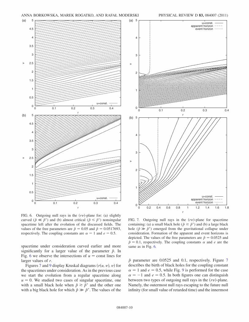
Figures 7 and 9 display Kruskal diagrams ðrðu; vÞ; vÞ forthe spacetimes under consideration. As in the previous casewe start the evolution from a regular spacetime alongu ¼ 0. We studied two cases of singular spacetime, onewith a small black hole when ~p * ~p� and the other onewith a big black hole for which ~p � ~p�. The values of the

~p parameter are 0.0525 and 0.1, respectively. Figure 7describes the birth of black holes for the coupling constant� ¼ 1 and e ¼ 0:5, while Fig. 9 is performed for the case� ¼ �1 and e ¼ 0:5. In both figures one can distinguishbetween two types of outgoing null rays in the ðrvÞ-plane.Namely, the outermost null rays escaping to the future nullinfinity (for small value of retarded time) and the innermost

0

0.5

1

1.5

2

2.5

3

3.5

4

4.5

5

0 0.1 0.2 0.3 0.4

v

r

(a)

u=const.

0

0.5

1

1.5

2

2.5

3

3.5

4

4.5

5

0 0.1 0.2 0.3 0.4

v

r

(b)

u=const.

FIG. 6. Outgoing null rays in the ðrvÞ-plane for: (a) slightlycurved (~p � ~p�) and (b) almost critical (~p & ~p�) nonsingularspacetime left after the evolution of the discussed fields. Thevalues of the free parameters are ~p ¼ 0:05 and ~p ¼ 0:0517693,respectively. The coupling constants are � ¼ 1 and e ¼ 0:5.

0

1

2

3

4

5

0 0.1 0.2 0.3 0.4

v

r

(a)u=const.

apparent horizonevent horizon

0

1

2

3

4

5

0 0.2 0.4 0.6 0.8 1 1.2 1.4 1.6 1.8

v

r

(b)

u=const.apparent horizon

event horizon

FIG. 7. Outgoing null rays in the ðrvÞ-plane for spacetimecontaining: (a) a small black hole (~p * ~p�) and (b) a large blackhole (~p � ~p�) emerged from the gravitational collapse underconsideration. Formation of the apparent and event horizons isdepicted. The values of the free parameters are ~p ¼ 0:0525 and~p ¼ 0:1, respectively. The coupling constants � and e are thesame as in Fig. 6.

ANNA BORKOWSKA, MAREK ROGATKO, AND RAFAŁ MODERSKI PHYSICAL REVIEW D 83, 084007 (2011)

084007-10

null rays which stem from the nonsingular axis r ¼ 0 andterminate at the singular part of the hypersurface r ¼ 0.Their evolution is described by finite value of v. Contraryto Refs. [13,14] we did not find in our numerical simula-tions intermediate outgoing null rays approaching a fixedradius at late times (when v ! 1). Just, the evolution inquestion resembles formation of a Schwarzschild blackhole, rather than an RN one with Cauchy horizon.

In order to better understand the causal structure of thedynamical spacetimes in question we shall proceed to

perform the Penrose diagrams (the dependence ðu; vÞ alongr ¼ const). In Figs. 10 and 12 we present the results for theslightly curved and almost critical nonsingular spacetimesfor � ¼ 1 or � ¼ �1 and e ¼ 0:5. The other parametersare as in Figs. 6 and 8, respectively. For both of them theoutermost contour line corresponding to r ¼ 0 is a non-singular straight line. On the other hand, in Figs. 11 and 13we presented lines of constant r in the ðvuÞ-plane for a

0

0.5

1

1.5

2

2.5

3

3.5

4

4.5

5

0 0.5 1 1.5 2 2.5

v

r

(a)

u=const.

0

0.5

1

1.5

2

2.5

3

3.5

4

4.5

5

0 0.5 1 1.5 2 2.5

v

r

(b)

u=const.

1.6

1.8

2

2.2

2.4

2.6

0 0.05 0.1

FIG. 8. Outgoing null rays in the ðrvÞ-plane for: (a) slightlycurved and (b) almost critical nonsingular spacetime left afterthe evolution of the fields in question. The free parameters aretaken to be ~p ¼ 0:0485 and ~p ¼ 0:0503946, respectively. Thecoupling constants are � ¼ �1 and e ¼ 0:5.

0

1

2

3

4

5

0 0.5 1 1.5 2 2.5

v

r

(a)

u=const.apparent horizon

event horizon

1.4

1.6

1.8

2

2.2

2.4

0 0.05 0.1 0.15

0

1

2

3

4

5

0 0.2 0.4 0.6 0.8 1 1.2 1.4 1.6 1.8

v

r

(b)

u=const.apparent horizon

event horizon

FIG. 9. Outgoing null rays in the ðrvÞ-plane for spacetimecontaining: (a) a small and (b) a large black hole emergedfrom the gravitational collapse under consideration. Formationof an apparent and an event horizons is depicted. The values ofthe free parameters are ~p ¼ 0:0525 and ~p ¼ 0:1. The values ofthe coupling constants are the same as in Fig. 8.

COLLAPSE OF CHARGED SCALAR FIELD IN DILATON . . . PHYSICAL REVIEW D 83, 084007 (2011)

084007-11

small and large black hole emerging from the gravitationalcollapse. Figure 11 was performed for � ¼ 1, while inFig. 13 we put the coupling constant � ¼ �1. In bothcases one has e ¼ 0:5. The outermost thick line is equiva-lent to r ¼ 0. Contrary to the previous cases, in the space-time of dynamical formation of a black hole one has astraight line (u ¼ v) in the left section. This behaviorcorresponds to the nonsingular axis. On the other hand,

the right part corresponds to the central singularity atr ¼ 0. Because of the fact that r;v < 0 along the latter

section, we have to do with the spacelike singularity.Two types of horizons are present in the singular space-times. The apparent horizon is represented by the contourr;v ¼ 0, while the event horizon is provided by the line of

constant u and characterized by r;v ¼ 0 when v ! 1. The

FIG. 10. Lines of constant r in the ðvuÞ-plane for: (a) a slightlycurved and (b) an almost critical nonsingular spacetime left afterthe evolution of the discussed fields. The values of the freeparameters and coupling constants are the same as in Fig. 6.

FIG. 11. Lines of constant r in the ðvuÞ-plane for spacetimecontaining: (a) a small and (b) a large black hole emerged fromthe considered gravitational collapse. Formation of an apparentand an event horizon and the position of singularity are shown.The values of the free parameters and the coupling constants arethe same as in Fig. 7.

ANNA BORKOWSKA, MAREK ROGATKO, AND RAFAŁ MODERSKI PHYSICAL REVIEW D 83, 084007 (2011)

084007-12

dynamical character of the emerging spacetimes is re-flected in relative positions of the aforementioned hori-zons. They do not coincide in the early stages of theevolution and in the end, they approach the same valueof u ¼ const as v tends to infinity.

The next object of our interest was an influence of thedilatonic coupling constant on the evolution described bythe considered equations of motion. The set of Penrose

diagrams (representing lines r ¼ const in the ðvuÞ-plane)for different values of � is shown in Fig. 14. The values ofdilatonic coupling constants were arbitrarily chosen to be0:5,1 and1:5. The value of the free family parameterwas taken as ~p ¼ 0:075. We conclude that the value of� exerts no qualitative influence on the structure of

FIG. 12. Lines of constant r in the ðvuÞ-plane for: (a) a slightlycurved and (b) an almost critical nonsingular spacetime left afterthe evolution of the fields in question. The values of the freeparameters and coupling constants are the same as in Fig. 8.

FIG. 13. Lines of constant r in the ðvuÞ-plane for spacetimecontaining: (a) a small and (b) a large black hole emerged fromthe gravitational collapse under consideration. Formation of anapparent and an event horizon as well as the position of singu-larity are shown. The values of the free parameters and thecoupling constants are the same as in Fig. 9.

COLLAPSE OF CHARGED SCALAR FIELD IN DILATON . . . PHYSICAL REVIEW D 83, 084007 (2011)

084007-13

FIG. 14. Lines of constant r in the ðvuÞ-plane for various values of coupling constant �.

ANNA BORKOWSKA, MAREK ROGATKO, AND RAFAŁ MODERSKI PHYSICAL REVIEW D 83, 084007 (2011)

084007-14

spacetime. The most striking effect is connected with themoment of the horizon’s formation. In general, for biggerabsolute values of � the horizon forms at earlier advancedtimes. Although the effect is far more noticeable for posi-tive values of dilatonic coupling constant, it is also presentfor � not exceeding zero.

We also examined the mass of a black hole emergingfrom the gravitational collapse in question as a function ofthe v-coordinate along the apparent horizon for differentvalues of coupling constant�. The relations are depicted inFigs. 15 and 16. Mass of a black hole, denoted by M, isHawking mass (56) calculated along the apparent horizon.It turned out that for large values of retarded time blackhole mass tends to a constant value. For positive values of� we observe that the bigger coupling constant is thebigger Hawking mass one gets. Moreover, the dependenceof M on the �-coupling constant is linear. In the case of �less than zero, its influence on the asymptotic value ofHawking mass is not so straightforward.

Now we proceed to study different features of the col-lapsing spacetimes as functions of null coordinates.Namely, we shall concentrate on Hawking mass (56),Ricci scalar (57), metric coefficient guv and v-derivativeof r. In our considerations we put ~p ¼ 0:1, e ¼ 0:5 andconsidered two distinct types of evolutions for dilatoniccoupling constants equal to � ¼ 1. We took into accountfoliations of spacetime in both v- and u-directions andstudied ingoing null rays terminating at a nonsingularpart of r ¼ 0, outside event horizon and within it, as wellas at singular r ¼ 0. We paid attention to outgoing nullrays outside, inside and exactly along the event horizon of

the emerging black hole. For both values of � we examineingoing null ray v ¼ 0:75 lying entirely outside the eventhorizon, hence terminating at the nonsingular part ofr ¼ 0. Next, we consider a null ray situated along v ¼ 1which crosses the event horizon, but also ends at regularr ¼ 0. The other ingoing null rays are v ¼ 1:25 for� ¼ �1 and v ¼ 1:2 for � ¼ 1. They have the samecharacteristic as the previous one, but they are situatedmuch closer to the cusp on the Penrose diagram of thespacetime. We also consider two null rays terminating at

0

0.01

0.02

0.03

0.04

0.05

0.06

0.07

0.08

0.09

0.1

1.4 1.6 1.8 2 2.2 2.4

M

v

α=-5α=-1.1

α=-1α=-0.9α=-0.1

α=0

FIG. 15. Mass of a black hole as a function of the v-coordinatealong the apparent horizon for different negative values ofcoupling constant �.

0

0.05

0.1

0.15

0.2

0.25

1 1.2 1.4 1.6 1.8 2 2.2 2.4

M

v

(a)

α=5α=1.1

α=1α=0.9α=0.1

α=0

0.08

0.09

0.1

0.11

0.12

0.13

0.14

0 0.2 0.4 0.6 0.8 1 1.2 1.4 1.6

M

α

(b)

FIG. 16. The influence of positive values of coupling constant� on mass of emerging black hole: (a) mass as a function ofv-coordinate along the apparent horizon and (b) an asymptoticvalue of black hole mass (for v ¼ 3) as a function of couplingconstant �.

COLLAPSE OF CHARGED SCALAR FIELD IN DILATON . . . PHYSICAL REVIEW D 83, 084007 (2011)

084007-15

central singularity which lie along v ¼ 1:75 and v ¼ 2. Asfar as the outgoing null rays are concerned, one examinedthe outgoing null ray u ¼ 0:5 situated outside event hori-zon for � ¼ �1 and � ¼ 1. The event horizon is situatedalong u ¼ 0:8557 for � ¼ �1 and along u ¼ 0:6663 for� ¼ 1, so these null rays were the next objects of ourstudies. We also paid attention to u ¼ const lying beyondthe event horizon. They are situated along u ¼ 0:86,u ¼ 0:95 for � ¼ �1 and along u ¼ 0:67, u ¼ 0:75 for� ¼ 1.

Hawking mass as a function of u along null rays inquestion for � ¼ �1 and � ¼ 1 is shown in Fig. 17. For

both values of �, in the case of ingoing null rays terminat-ing at the nonsingular part of r ¼ 0, Hawking mass tends tozero as the retarded time increases. Its behavior along v ¼const is evidently different for ingoing null rays hitting thecentral singularity. For � ¼ �1 Hawking mass is constantuntil it reaches the vicinity of r ¼ 0, where it growsrapidly. The situation is quite different for the couplingconstant � ¼ 1. In this case Hawking mass grows contin-uously along v ¼ const and its increase is not so suddenclose to r ¼ 0.Hawking mass as a function of v along the aforemen-

tioned null rays for � ¼ �1 and� ¼ 1 is shown in Fig. 18.

0

0.05

0.1

0.15

0.2

0 0.2 0.4 0.6 0.8 1 1.2

m

u

(a)

v=0.75v=1

v=1.25v=1.75

v=2

0

0.05

0.1

0.15

0.2

0.25

0 0.2 0.4 0.6 0.8 1 1.2

m

u

(b)

v=0.75v=1

v=1.2v=1.75

v=2

FIG. 17. Hawking mass as a function of the u-coordinate alongingoing null rays for: (a) � ¼ �1 and (b) � ¼ 1.

0

0.02

0.04

0.06

0.08

0.1

0.12

0.14

0.16

0.5 1 1.5 2 2.5

m

v

(a)

u=0.5u=0.8557

u=0.86u=0.95

0.025

0.05

0.075

0.1

0.125

0.15

1.25 1.5 1.75 2

0

0.05

0.1

0.15

0.2

0.5 1 1.5 2 2.5

m

v

(b) u=0.5u=0.6663

u=0.67u=0.75

0

0.025

0.05

0.075

0.1

1.2 1.3 1.4 1.5

FIG. 18. Hawking mass as a function of the v-coordinate alongoutgoing null rays for: (a) � ¼ �1 and (b) � ¼ 1.

ANNA BORKOWSKA, MAREK ROGATKO, AND RAFAŁ MODERSKI PHYSICAL REVIEW D 83, 084007 (2011)

084007-16

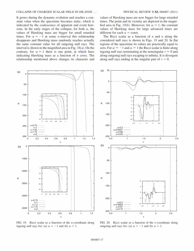
It grows during the dynamic evolution and reaches a con-stant value when the spacetime becomes static, which isindicated by the coalescence of apparent and event hori-zons. In the early stages of the collapse, for both �, thevalues of Hawking mass are bigger for small retardedtimes. For � ¼ �1 at some v-interval this relationshipdisappears and Hawking mass randomly reaches actuallythe same constant value for all outgoing null rays. Theinterval is shown in the magnified area in Fig. 18(a). On thecontrary, for � ¼ 1 there is one point, at which linesindicating Hawking mass as a function of v cross. Therelationship mentioned above changes its character and

values of Hawking mass are now bigger for large retardedtimes. The point and its vicinity are depicted in the magni-fied area in Fig. 18(b). Moreover, for � ¼ 1, the constantvalues of Hawking mass for large advanced times aredifferent for each u ¼ const.The Ricci scalar as a function of u and v along the

considered null rays is shown in Figs. 19 and 20. In flatregions of the spacetime its values are practically equal tozero. For� ¼ �1 and� ¼ 1 the Ricci scalar is finite alongingoing null rays terminating at the nonsingular r ¼ 0 andalong outgoing null rays escaping to infinity. It is divergentalong null rays ending at the singular part of r ¼ 0.

-300

-250

-200

-150

-100

-50

0

0 0.2 0.4 0.6 0.8 1 1.2 1.4

R

u

(a)

v=0.75v=1

v=1.25v=1.75

v=2

-10

-8

-6

-4

-2

0

0 0.2 0.4 0.6 0.8 1

-5000

-4000

-3000

-2000

-1000

0

0 0.2 0.4 0.6 0.8 1 1.2

R

u

(b)

v=0.75v=1

v=1.2v=1.75

v=2

-40

-30

-20

-10

0

0 0.2 0.4 0.6 0.8 1 1.2

FIG. 19. Ricci scalar as a function of the u-coordinate alongingoing null rays for: (a) � ¼ �1 and (b) � ¼ 1.

-250

-200

-150

-100

-50

0

50

0.5 1 1.5 2 2.5

R

v

(a)

u=0.5u=0.8557

u=0.86u=0.95

-20

-15

-10

-5

0

5

10

0.5 1 1.5 2 2.5

-250

-200

-150

-100

-50

0

0.5 1 1.5 2 2.5

R

v

(b)

u=0.5u=0.6663

u=0.67u=0.75

-10

-5

0

5

10

0.5 1 1.5 2 2.5

FIG. 20. Ricci scalar as a function of the v-coordinate alongoutgoing null rays for: (a) � ¼ �1 and (b) � ¼ 1.

COLLAPSE OF CHARGED SCALAR FIELD IN DILATON . . . PHYSICAL REVIEW D 83, 084007 (2011)

084007-17

On the other hand, the metric coefficient guv as a func-tion of u and v along the null rays in question is shown inFigs. 21 and 22. For both values of � it is constant inflat regions of spacetime. In curved areas it is slightlyincreasing with the retarded time for ingoing null raysterminating at a regular part of r ¼ 0 and considerablydecreasing in the other case. guv has a peak near thevalue of the advanced time, where the apparent horizonappears and the spacetime becomes singular. The peaks for

both values of � are shown in magnified areas of therespective figures. Then, guv decreases with the advancedtime along all outgoing null rays. The changes are rathersmall outside the apparent horizon and become large be-yond it.The derivative of r with respect to v as a function of u

along null rays in question is shown in Fig. 23. It is constantor slightly decreasing for ingoing null rays lying outsidethe apparent horizon and displays a strong variability along

-45

-40

-35

-30

-25

-20

-15

-10

-5

0

0 0.2 0.4 0.6 0.8 1 1.2

g uv

u

(a)

v=0.75v=1

v=1.25v=1.75

v=2

-0.7

-0.6

-0.5

-0.4

-0.3

-0.2

0 0.2 0.4 0.6 0.8 1 1.2

-30

-25

-20

-15

-10

-5

0

0 0.2 0.4 0.6 0.8 1 1.2

g uv

u

(b)

v=0.75v=1

v=1.2v=1.75

v=2

-1

-0.8

-0.6

-0.4

-0.2

0 0.2 0.4 0.6 0.8 1 1.2

FIG. 21. Metric coefficient guv as a function of theu-coordinate along ingoing null rays for: (a) � ¼ �1 and (b)� ¼ 1.

-100

-80

-60

-40

-20

0

0.5 1 1.5 2 2.5 3 3.5 4 4.5 5

g uv

v

(a)

u=0.5u=0.8557

u=0.86u=0.95

-2

-1.5

-1

-0.5

0.5 1 1.5 2 2.5 3 3.5

-6

-5

-4

-3

-2

-1

0

0.5 1 1.5 2 2.5 3 3.5 4 4.5 5

g uv

v

(b)

u=0.5u=0.6663

u=0.67u=0.75

-0.7

-0.6

-0.5

0.5 1 1.5 2 2.5 3 3.5

FIG. 22. Metric coefficient guv as a function of thev-coordinate along outgoing null rays for: (a) � ¼ �1 and(b) � ¼ 1.

ANNA BORKOWSKA, MAREK ROGATKO, AND RAFAŁ MODERSKI PHYSICAL REVIEW D 83, 084007 (2011)

084007-18

v ¼ const, which crosses the apparent horizon. On theother hand, the derivative of r with respect to v as afunction of v along the examined null rays is shown inFig. 24. It is constant in the v-interval corresponding to thenonsingular part of r ¼ 0. In the region, where the lineindicating a central singularity on Penrose diagram is thesteepest r;v decreases rapidly, but not uniformly—it in turn

displays quick and slow changes. In the area, where thesingular r ¼ 0 lies almost along a constant u the derivativeof r with respect to v changes only a little. It increases foroutgoing null rays outside the event horizon, is constantalong it, and decreases within it.

V. CONCLUSIONS

In our paper we considered a dynamical collapse of acharged complex scalar field in the low-energy limit of thestring theory, the so-called dilaton gravity. In order to solvethe complicated equations of motion one used the double-null coordinates which enabled us to begin with the regularinitial spacetime at null infinity, compute the formation of ablack hole, and broaden our inspection to the singularityformed during the dynamical collapse in question. We haveformulated the problem under consideration as a system ofthe first-order partial differential equations with the ade-quate boundary and regularity conditions.

-16

-14

-12

-10

-8

-6

-4

-2

0

0 0.2 0.4 0.6 0.8 1 1.2

r ,v

u

(a)

v=0.75v=1

v=1.25v=1.75

v=2

-0.2

-0.1

0

0.1

0.2

0.3

0.4

0.5

0 0.2 0.4 0.6 0.8 1 1.2

-16

-14

-12

-10

-8

-6

-4

-2

0

0 0.2 0.4 0.6 0.8 1 1.2

r ,v

u

(b)

v=0.75v=1

v=1.2v=1.75

v=2

-0.4

-0.2

0

0.2

0.4

0 0.2 0.4 0.6 0.8 1 1.2

FIG. 23. Quantity r;v as a function of the u-coordinate alongingoing null rays for: (a) � ¼ �1 and (b) � ¼ 1.

-14

-12

-10

-8

-6

-4

-2

0

0.5 1 1.5 2 2.5 3 3.5 4 4.5 5

r ,v

v

(a)

u=0.5u=0.8557

u=0.86u=0.95

-1.5

-1

-0.5

0

0.5

0.5 1 1.5 2 2.5 3 3.5 4 4.5 5

-1

-0.8

-0.6

-0.4

-0.2

0

0.2

0.4

0.6

0.5 1 1.5 2 2.5 3 3.5 4 4.5 5

r ,v

v

(b)

u=0.5u=0.6663

u=0.67u=0.75

-0.6

-0.4

-0.2

0

0.2

0.4

0.6

0.5 1 1.5 2 2.5 3 3.5

FIG. 24. Quantity r;v as a function of the v-coordinate alongoutgoing null rays for: (a) � ¼ �1 and (b) � ¼ 1.

COLLAPSE OF CHARGED SCALAR FIELD IN DILATON . . . PHYSICAL REVIEW D 83, 084007 (2011)

084007-19

We begin our numerical studies with a subcritical evo-lution. One observes that there is a flat region in theðrvÞ-plane corresponding to small values of advancedand retarded coordinates where rðu; vÞ is proportional tou and v-coordinates. Then, the curvature of the spacetimecomes into being, destroying this behavior. The spacetimecurved earlier and more significantly for the larger valuesof the ~p parameter. Next we proceed to analyze the Kruskaldiagrams ðr; vÞ along u ¼ const for the considered space-times. We found that the outermost null rays escaped to thefuture null infinity, while the innermost originating fromthe nonsingular axis r ¼ 0 terminated at the singular partof the hypersurface in question. We did not observe for-mation of the inner horizon. The causal structure of thedynamical collapse was elaborated by means of Penrosediagrams, namely, we analyzed ðv; uÞ-dependence alongr ¼ const. We noticed that the left part of the diagramcorresponded to the nonsingular axis r ¼ 0 and the rightsection of it was bounded with the central singularity. Wehave indicated two types of the horizons, i.e., the apparentone represented by the contour r;v ¼ 0 and the event

horizon forming when v ! 1. They did not coincide atthe early stages of the dynamical collapse but in the endthey approached the same value of u-coordinate as v ! 1.Penrose diagrams for various values of� coupling constantwere also found.

On the other hand, we considered Hawking mass as afunction of v-coordinate along different null rays. It turned

out that it grew during the dynamic collapse and reachedthe constant value for a static spacetime, where the coales-cence of the apparent and event horizon took place. Wealso analyzed the behavior of Hawking mass as a functionof ingoing null rays terminating at a nonsingular part ofr ¼ 0. It was revealed that it tended to zero with thepassage of the retarded time. Hawking mass behavior,along v ¼ const for ingoing null rays hitting the centralsingularity, was different for the different values of cou-pling constant �. As far as the Ricci scalar and metrictensor coefficient guv are concerned their behavior is moreor less similar for the positive and negative � couplingconstant.To conclude one remarks that the dynamical collapse

of a complex charged scalar field in the realm ofdilaton gravity resembles the collapse leading to theSchwarzschild black hole rather than the collapse ofcharged field in Einstein-Maxwell theory. Though, whenwe check our code and put dilaton field and couplingconstant equal to zero we get the behavior leading to ablack hole with an a Cauchy horizon; during dynamicalcollapse of charged scalar field in dilaton theory we do notfind the inner black hole horizon.

ACKNOWLEDGMENTS

A.B.was supported by theHumanCapital Programmeofthe European Social Fund sponsored by European Union.

[1] S.W. Hawking and G. F. R. Ellis, The Large ScaleStructure of Space-time (Cambridge University Press,Cambridge, England, 1973).

[2] V. A. Belinsky, I.M. Khalatnikov, and E.M. Lifshitz, Adv.Phys. 19, 525 (1970).

[3] V. A. Belinsky and I.M. Khalatnikov, Zh. Eksp. Teor. Fiz.74, 3 (1978).

[4] T. Damour and M. Henneaux, Phys. Lett. B 488, 108(2000); Phys. Rev. Lett. 85, 920 (2000).

[5] A. Ori, Phys. Rev. Lett. 67, 789 (1991); 68, 2117 (1992);L.M. Burko and A. Ori, Phys. Rev. Lett. 74, 1064 (1995),A. Ori and D. Gorbonos, J. Math. Phys. (N.Y.) 48, 092502(2007); D. Gorbonos and G. Wolansky, J. Math. Phys.(N.Y.) 48, 092503 (2007).

[6] P. R. Brady and J. D. Smith, Phys. Rev. Lett. 75, 1256(1995).

[7] W.A. Hiscock, Phys. Lett. A 83, 110 (1981).[8] E. Poisson and W. Israel, Phys. Rev. D 41, 1796 (1990);

Phys. Rev. Lett. 63, 1663 (1989).[9] M. L. Gnedin and N.Y. Gnedin, Classical Quantum

Gravity 10, 1083 (1993).[10] L.M. Burko, Phys. Rev. Lett. 79, 4958 (1997).[11] L.M. Burko and A. Ori, Phys. Rev. D 57, R7084 (1998).

[12] S. Ayal and T. Piran, Phys. Rev. D 56, 4768(1997).

[13] S. Hod and T. Piran, Phys. Rev. Lett. 81, 1554 (1998);Gen. Relativ. Gravit. 30, 1555 (1998).

[14] Y. Oren and T. Piran, Phys. Rev. D 68, 044013(2003).

[15] J. Hansen, A. Khokhlov, and I. Novikov, Phys. Rev. D 71,064013 (2005).

[16] E. Sorkin and T. Piran, Phys. Rev. D 63, 084006(2001).

[17] E. Sorkin and T. Piran, Phys. Rev. D 63, 124024 (2001).[18] S. E. Hong, D. Hwang, E. D. Stewart, and D. Yeom,

Classical Quantum Gravity 27, 045014 (2010).[19] D. Hwang and D. Yeom, Classical Quantum Gravity 27,

205002 (2010).[20] D. Hwang and D. Yeom, arXiv:gr-qc1010.2585.[21] E. Sorkin, Phys. Rev. D 81, 084062 (2010).[22] A. Doroshkevich, J. Hansen, D. Novikov, I. Novikov, D.

Park, and A. Shatskiy, Phys. Rev. D 81, 124011 (2010).[23] M. Heusler, Black Holes Uniqueness Theorems

(Cambridge University Press, Cambridge, England,1996); K. S. Thorne, Black Holes and Time Warps (W.W. Norton and Company, New York, 1994).

ANNA BORKOWSKA, MAREK ROGATKO, AND RAFAŁ MODERSKI PHYSICAL REVIEW D 83, 084007 (2011)

084007-20

[24] A. K.M. Masood-ul-Alam, Classical Quantum Gravity 10,2649 (1993); M. Rogatko, Classical Quantum Gravity 14,2425 (1997); M. Rogatko, ibid. 19, 875 (2002); M. Marsand W. Simon, Adv. Theor. Math. Phys. 6, 279 (2003); M.Rogatko, Phys. Rev. D 58, 044011 (1998); M. Rogatko,ibid. 59, 104010 (1999); M. Rogatko, ibid. 82, 044017(2010); S. Yazadijev, ibid. 82, 124050 (2010).

[25] R. Moderski and M. Rogatko, Phys. Rev. D 63, 084014(2001); 64, 044024 (2001); 72, 044027 (2005); M.Rogatko, ibid. 75, 104006 (2007); R. Moderski and M.Rogatko, ibid. 77, 124007 (2008); G. Gibbons and M.

Rogatko, ibid. 77, 044034 (2008); M. Gozdz, L.Nakonieczny, and M. Rogatko, ibid. 81, 1040027 (2010).

[26] D. Christodoulou, Commun. Pure Appl. Math. 46, 1131(1993).

[27] R. S. Hamade and J.M. Stewart, Classical QuantumGravity 13, 497 (1996).

[28] M.W. Choptuik, Phys. Rev. Lett. 70, 9(1993).

[29] C. Gundlach, Phys. Rep. 376, 339 (2003).[30] A. V. Frolov and U. Pen, Phys. Rev. D 68, 124024

(2003).

COLLAPSE OF CHARGED SCALAR FIELD IN DILATON . . . PHYSICAL REVIEW D 83, 084007 (2011)

084007-21