Cointegration analysis of the impact of Azerbaijan and

274

Orudzhev, E., & Alizade, A. (2021). Cointegration analysis of the impact of Azerbaijan and Ukraine GDPs on the trade turnover between these countries. Journal of International Studies, 14(3), 274-290. doi:10.14254/2071-8330.2021/14-3/18

Cointegration analysis of the impact of Azerbaijan and Ukraine GDPs on the trade turnover between these countries

Elshar Orudzhev

Department of Mathematical Economy,

Baku State University (BSU),

Azerbaijan

[email protected]

ORCID 0000-0002-6985-1407

Arzu Alizade

Department of World Economy,

Baku State University (BSU),

Azerbaijan

[email protected]

ORCID 0000-0002-0237-356X

Abstract. This article studies the integration processes between Azerbaijan and

Ukraine by using the indicators of the integratedness of the GDPs of these

countries and of the trade turnover between them. The annual data from 1994 to

2018 are studied as the period of monitoring. All the studied time series are non-

stationary, and in passing to the time series of differences, they retain only the

information corresponding to short-term changes in their dynamics; while

information about long-term changes in the process, contained in those levels of

variables that are lost in the transition to differences, is lost. Therefore, problems

of correct modelling of the corresponding time series, of which components lead

to departure from stationarity, arise. The article uses the econometric

methodology of the gravity modelling of the correlation between non-stationary

time series. In the modelling, econometric methods, all the necessary step-by-step

statistical procedures to determine the order of integratedness of the non-

stationary time series, to identify the assessment of the parameters of the model

and to check its adequacy and the accuracy of short-term and long-term predicted

values are correctly used by applying Excel tools and the Eviews package. The

departure of empirical tests from the trend is analyzed. The constructed dynamic

analogue of the gravity model enables to qualitatively predict the status of

integration of the foreign trade of the studied two countries. Based on the

constructed model, econometrically sound recommendations that enable a

dynamic analysis of effective regulation of the export and import transactions

Received: August, 2020 1st Revision:

February, 2021 Accepted:

September, 2021

DOI: 10.14254/2071-

8330.2021/14-3/18

Journal of International

Studies

Sci

enti

fic

Pa

pers

© Foundation of International

Studies, 2021 © CSR, 2021

mailto:[email protected]

mailto:[email protected]

Elshar Orudzhev, Arzu Alizade

Cointegration analysis of the impact of Azerbaijan and Ukraine GDPs on the trade …

275

between these countries by the governments to balance the mutual trade have

been developed.

Keywords: cointegration, analogue of the gravity model, error correction mechanism,

Johansen tests, dispersion decomposition, impulse response function, GDP,

trade turnover, Ukraine, Azerbaijan

JEL Classification: C000, C010, C020, C100, C530, C590

1. INTRODUCTION

The article is dedicated to the research of trade cointegratedness processes of foreign economic activity

between Azerbaijan and Ukraine. By cointegratedness processes here we mean that the corresponding

realizations of the non-stationary time series of the integratedness indicators of these countries are

cointegrated up to a certain order of differences (Verbeek, 2012). For the assessment of integration

processes criteria for the integratedness of trade markets, the scale of cross-border flows of goods, services,

capital, etc. are widely used. If there is a convergence of indicators in a promising time period, then we can

assume that the integratedness processes are effective. The problem of developing trade and economic

integration of Azerbaijan with Ukraine doesn’t lose its relevance thus far. There is a huge unused potential

for the comprehensive development of Ukrainian-Azerbaijani trade and economic relations. Despite the

fact that over the past two years, the trade turnover between these countries has had positive trends, the

absolute figures are unsatisfactory based on the potential of mutual trade. It should be noted that Ukraine

is one of the main partners of Azerbaijan. It ranks second in the total trade in the post-soviet area, after

Russia. In 2015, in terms of the volume of trade in goods and services with Ukraine, Azerbaijan ranked fifth

among the CIS countries, after Russia, Belarus, Kazakhstan and Moldova. In connection with the

deterioration of Russian-Ukrainian relations and the difficult geopolitical in the Donbass region, after a

threefold decrease in the volume of trade between Ukraine and Azerbaijan in 2014-2016, from 979 million

USD to 321 million USD, in 2018 already this turnover increased to approximately 360 million USD. The

decrease in commodity turnover is primarily due to the fact that in the Donbass, the industrial center of

Ukraine, which traditionally supplied metal products to Azerbaijan, due to the ongoing military conflicts the

factories worked intermittently. Another reason is a number of restrictions imposed by Russia on the transit

of Ukrainian products through its territory after Ukraine ratified the agreement on the free trade zones with

the EU. We should state that trade in goods between Azerbaijan and Ukraine in 2010 amounted to about 1

billion USD. Until 2010, the trade balance in bilateral relations was invariably in favor of Ukraine. It is

necessary to return the lost indicators at an accelerated pace, and then bring the trade cooperation to a new

level. From the statistical data, it turns out that if Azerbaijan's foreign trade turnover with Ukraine was only

350 mln USD in 2006 (with a specific weight of 3.1%), then this figure was 1 billion 354 mln USD in 2010

(with a specific weight of 4.8%). The specific weight of Ukraine in the import of Azerbaijan was 6% in 2006.

The amount of goods imported from Ukraine in monetary terms increased from 317.5 mln USD to 465.6

mln USD in 2006, with a specific weight of 7.1% in 2010. The specific weight of Ukraine in the export of

the republic of Azerbaijan was only 0.6% in 2006. Due to the expansion of cooperation, in 2010 the export

of Azerbaijan to Ukraine with a specific weight of 4.2% took the first place among the CIS republics. It is

necessary to return the lost indicators at an accelerated pace, and then bring trade cooperation to a new

level. Today Azerbaijan's export to Ukraine is largely formed by the energy carriers.

The export of crude oil from Azerbaijan to Ukraine is mainly supplier to the Kremenchug refinery. In

addition to crude oil, Azerbaijan also supplies aviation kerosene, motor oils, some types of diesel fuel,

Journal of International Studies

Vol.14, No.3, 2021

276

petroleum coke, refrigeration compressors, etc. To Ukraine. In addition, fruits and vegetables, juices, canned

food, soft drinks, etc. are imported from Azerbaijan to Ukraine. At the same time, Ukraine supplies to

Azerbaijan metals and metal products, electric machines, meat, dairy and confectionery products, drinks,

etc. In the structure of Ukrainian exports to Azerbaijan, the share of ferrous metallurgy and other non-

precious metals is significant. These supplies were mainly from the Ilyich Iron and Steel Works of Mariupol,

ArcelorMittal Kryvyi Rih and from the factories operating mainly in Donetsk and Luhansk regions. It is

necessary to diversify trade and economic relations between these countries in all the spheres of the

economy, including tourism, international transport and logistics activities, one of the priority areas of which

is the projects of the east-west and north-south transport corridors as well as the Odessa-Brody project

which opens up new opportunities for the development of Ukrainian economy. It is important to further

strengthen the trade, economic and investment components of the bilateral cooperation, in particular,

through practical implementation of investment projects in Ukraine with the participation of Azerbaijani

business and vice versa. It is also necessary to provide more favorable trade regimes to each other (revision

of transport and customs tariffs) in the context of the global shocks associated with the coronavirus

(COVID-19), and closer inter-country economic cooperation in the non-oil sector. The possibilities of

mutual complementary cooperation in the aviation and space spheres should also be considered, taking into

account the course of Azerbaijan towards the development of these areas and the scientific potential

available in Ukraine.

To assess the prospects for expanding mutually beneficial factors in trade, economic, fuel and energy

and transport spheres, a highly relevant task is to conduct an econometric co-integration analysis of the

mutual influence of the corresponding aggregated indicators of foreign trade of the two strategic partners.

Here, the studied integration processes between Azerbaijan and Ukraine are considered by using the

indicators of Azerbaijan's GDP and the trade turnover of this country with Ukraine. These indicators are

the most significant variables for analyzing the dynamics of mutual trade turnover in the environment of

inter-country cooperation and for assessing the impact of the mutual trade on their inclusive growth. The

nominal data with the unit of measurement in thousands USD was used while the monitored period is from

1994 to 2018. The major data sources have been the Statistical Committee of the Republic of Azerbaijan

and the World Bank (www.stat.gov.az; www.worldbank.com).

2. ANALYSIS OF RECENT PUBLICATIONS.

In recent years, a number of articles have been published devoted to the study of integration processes

in the Common Free Market Zone (Russia, Belarus and Kazakhstan), in the EAEU, between individual and

groups of post-Soviet countries, taking into account their regional characteristics in the process of the

transformation of the economies (Andronova, 2012; Pylin, 2015; Orudzhev & Huseynova, 2019; Orudzhev

& Huseynova, 2020). In these articles, as a result of the study of indicators of mutual trade by methods of

comprehensive economic and statistical analysis, trends in the development of trade and economic

cooperation of the studied countries are brought to light, and the main directions for improving the

integrated economic processes are identified. In particular, in (Orudzhev & Huseynova, 2019) the

cointegration ratios of the mutual influences of Azerbaijan's GDP and the balance of export-import

operations of Russia and Belarus are found. Due to the heterogeneity of the time series in (Orudzhev &

Huseynova, 2019), the predicted errors of the trend regression models turned out to be high. The

cointegration analysis of Azerbaijan's trade relations with the main members of the EAEU is studied in

(Orudzhev & Huseynova, 2020). As a result of the obtained quantitative estimates of the dispersion of the

GDP aggregate of Azerbaijan's economic development, the positive impact on economic growth of the

foreign trade with these countries, which are characterized by regional disproportions in economic



277

development, is determined. And in Article (Golovan, 2012), the dynamics of the structure of Ukraine's

foreign trade from 2005 to 2011 is analyzed. It establishes relationship between the geographical structure

of the foreign trade both with external debt and the unfavorable commodity structure of Ukraine's foreign

trade. Studies (Kharlamova & Vertelieva, 2013) are devoted to the statistical analysis of the international

competitiveness of Ukraine and 29 states (the analysis doesn’t include Azerbaijan) based on data from 2004

to 2013. Clusters of countries are identified by the level of their relative national competitiveness. Article

(Chebotareva & Fayzulina, 2016) provides a description of the main trends in the development of Ukraine's

foreign trade, the geographical structure of exports and imports of goods, and a correlation analysis of the

impact of exports and imports on the formation of Ukraine's GDP. It is stated that the main partner, both

in import and export, for many years has been Russia, the economic and political relations with which are

currently going through hard times. Trade wars, conflicts in the east of Ukraine forced the participants of

the foreign economic activities, both Ukraine and Russia, to look for trading partners in other countries.

The authors of Article (Moroz et al., 2017) studied the current state and prospects of the trade relations

between Ukraine and the Visegrad countries. Corresponding econometric models of trade flows between

Ukraine and these countries are built. In (Frolov & Savytska, 2016), the cause and effect relationships

between the components of the region's foreign trade turnover and indicators that characterize the

economic situation of the region, the country and the world are studied. The export of the Sumy region is

analyzed as an example. In Article (Kalyuzhna, 2020) a retrospective analysis of Ukraine's foreign trade in

goods in the context of deepening interstate economic contradictions is carried out. An empirical analysis

of the absolute indicators (the volume of the trade turnover in general and with individual groups of

countries) and relative indicators (the share of trade with individual groups of countries in the overall

structure of the trade turnover) of Ukraine's foreign trade in goods with the countries of the European

Union and the CIS is carried out. This work doesn't study the trade in goods with Azerbaijan. And in Article

(Orudzhev & Alizade, 2020) using the posteriori approach, in case the total number of factors influencing

Azerbaijan's GDP is significant, an econometric analysis is carried out from a variety of insignificant factors.

Here, the cause and effect relationship with only one element of this set (with the trade turnover of Ukraine)

is studied. Estimates of the parameters of the econometric model are found, after which, using the error

correction model, qualitative dynamic statistical characteristics are determined. It is also possible to build a

similar model for Ukraine's GDP in the context of the trade turnover with Azerbaijan and compare the

corresponding model options for the entire range of characteristics of their quality for the purposes of

forecasting. Using the reverse transformation, we can state that the quantitative correlations found in

(Orudzhev & Alizade, 2020) make it possible to build a dynamic model of long-term relationship and predict

the performance of the main factors. In this case, exports and imports depend on the aggregate

macroeconomic indicators of both countries, primarily on the size of their economies, which are

traditionally characterized by the gross domestic product, gross capital formation, imports and exports, and

possible dependence on some other factors.

3. METHODOLOGY

The article uses an econometric methodology for studying the statistical relationship between

multidimensional non-stationary time series, including Engle – Granger and Johansen cointegration tests,

research of Granger causality, responses to shock (Hall, 1992). Based on the vector error correction model

(VECM), and performing decomposition of the residual variance of forecast errors. For the theoretical

analysis of modeling calculations, we used the methods of multivariate statistical analysis (Verbeek,2012),

necessary for constructing multidimensional data models (multivariate analysis of dispersion, multivariate

correlation and regression analysis, statistical hypotheses in the analysis of multivariate data), four-


Vol.14, No.3, 2021

278

dimensional vector models of auto-regression and co-integration in these models, approaches of modern

economic and mathematical modeling (Verbeek, 2012), and application packages Excel (Kenneth & Carey,

2010) and EViews (Johnson, 2015).

4. THE MAIN RESULTS OF THE RESEARCH

In this article, the forecast of the relationship between the integratedness indicators of the GDP of

Azerbaijan and Ukraine and trade turnover between these countries is carried out by the method of

logarithmic approximation of the actual data with subsequent extrapolation. In this case, the multiplicative-

power relation is considered as the initial dependence:

𝑦𝑡 = 𝛼0 𝑥𝑡1𝛼1𝑥𝑡2

𝛼2𝑑𝛼3 , 𝑡 = 1,25. (1)

Models of the dependence of the trade turnover 𝑦𝑡 between Azerbaijan and Ukraine on the factor 𝑥𝑡1,

representing the GDP of Azerbaijan and the factor 𝑥𝑡2, representing the GDP of Ukraine, with a random

term 𝜀𝑡, which includes the total influence of all factors not accounted for in the model, measurement errors

and geographic distance d (in thousand kilometers) between Baku and Kiev. 𝛼0- free member, 𝛼1, 𝛼2, 𝛼3-

constant number in this formula. Here the main factorial elements are combined by the multiplication

operation.It’s assumed that, 𝛼1 > 0, 𝛼2 > 0, 𝛼3 < 0.

Marks of constant values correspond to the assumptions about the directions of influence of GDP and

distance on the trade flow of the gravity model (Tinbergen, 1962), which is based on the assumption that

the volume of trade in goods between two countries is directly proportional to the capacity of their markets

and inversely proportional to the barriers between them. At the same time, the capacity of markets is

determined by the size of the GDP of trading partners, and the impact of barriers is approximated by the

geographical distance between countries.

As a direct proportionality, we can use the population size, area of countries, GDP per capita. However,

here, as factors influencing the trade turnover between Ukraine and Azerbaijan, the main macroeconomic

indicators GDP and the size of the economies of these countries are selected. But the results obtained in

this work are transferred to the case including these factors in the model without significant changes. Various

modifications of the gravity model for a certain type of product between two or more countries are

constructed in (Dankevych, Pyvovar & Dankevych, 2020)

It should also be noted that the specifications of models of foreign trade flows for sea, rail, road and

pipeline transportation are evaluated separately. The structure of transportation costs can include other

components, including the costs for coping with administrative barriers (customs procedures), membership

in currency and trade unions, and exchange rate volatility. We only study the above mentioned dependence

in this work.

The regression equation is linear with respect to the logarithms of the original variables, the model is

double logarithmic.

The power exponents of the factors of the model of this paper are estimates of the partial elasticity of

the effective factor with respect to causal factors.

The studied time series will be transformed into logarithmic ones. This transformation makes it

possible to more clearly represent the relationship between the indicators under consideration. The first

differences of the logarithms are an approximation of the growth rates of the corresponding variables.

Dynamic data descriptions from (www.stat.gov.az; www.worldbank.com) and descriptive statistics on

the logarithms of variables are shown in Graph 1 and Table 1:

http://www.stat.gov.az/

http://www.worldbank.com/



279

Graph 1. Dynamic descriptions of data

Source: The results of procedures realized in MS EXCEL 2010 software package

insert /Charts group/Line with Markers

Table 1

Descriptive statistics on the logarithms of variables

LNUKRT LNGDPAZ LNGDPUKR LNRESIDS

Mean 12.50237 16.58730 18.20031 -1.928520

Median 12.71052 16.85922 18.32671 -1.480693

Maximum 14.19880 18.13612 19.02669 -0.362492

Minimum 10.74011 14.30366 17.25791 -6.508979

Std. Dev. 1.057384 1.261864 0.590442 1.513119

Skewness -0.060990 -0.238608 -0.121725 -1.674268

Kurtosis 1.725032 1.529524 1.570301 5.268172

Jarque-Bera 1.708773 2.489621 2.190944 17.03886

Probability 0.425544 0.287995 0.334382 0.000200

Sum 312.5592 414.6826 455.0076 -48.21301

Sum Sq. Dev. 26.83344 38.21520 8.366930 54.94867

Observations 25 25 25 25

Source: The results of procedures realized in EViews 8 software package

As Group/View/Descriptive statistics/Common sample

Graph 1 visually comparing the dynamics of the logarithms of the studied variables over the considered

period. It can show no sharp structural shifts in either the constant or trend of the equation.

From table 1, it appears that the elements of the 2nd, 3rd, 4th columns have a slight left-sided

asymmetric of the empirical curves relative to the theoretical; for the element of the 5th column, the vertex

is shifted to the left significantly. Kurtosis for elements of the 2nd, 3rd, 4th columns appears that observe a

slight peaking of the empirical curve; for the 5th column, elements of this value increase approximately

three times, which leads to a significant deviation of the empirical distribution of residuals from the normal

one.

On the assumption of comparative analysis with the results of work (Orudzhev & Alizade, 2020),

Graph 1 and Table 1, it can be assumed that the dependence of the logarithm of Azerbaijan's foreign trade

turnover with Ukraine on the logarithms of GDP of these countries are described by the following linear

regression model.

𝑙𝑛𝑦𝑡 = 𝛼00 + 𝛼1𝑙𝑛𝑥𝑡1 + 𝛼2𝑙𝑛𝑥𝑡2 + 𝑙𝑛𝜀𝑡, 𝑡 = 1, 25 (2)

-10

-5

0

5

10

15

20

25

1994

1995

1996

1997

1998

1999

2000

2001

2002

2003

2004

2005

2006

2007

2008

2009

2010

2011

2012

2013

2014

2015

2016

2017

2018

Th

ou

san

d d

oll

ar

US

A

Years

[1]

[2]

[3]

[4]

[1]-LNGDPUKR[2]-LNGDPAZ[3]-LNUKRT


Vol.14, No.3, 2021

280

𝑦𝑡,𝑦𝑡 , 𝑥1𝑡, 𝑥2𝑡, 𝑥3𝑡 𝑥𝑡1, 𝑥𝑡2-relevant factors, 𝛼00 = 𝑙𝑛𝛼0 + 𝛼3𝑙𝑛𝑑, 𝛼1, 𝛼2𝛼0, 𝛼1, 𝛼2, 𝛼3-unknown

model parameters; 𝜀 – a random member, that includes the total influence of all factors unaccounted for in

the model, measurement errors.

For definiteness d=2,233 thousand km, 𝛼3 = −2. Transformation (1) into (2) leads to the

transformation of random deviations 𝜀𝑡 into 𝑙𝑛𝜀𝑡. The use of the least squares method (LSM) in (2) to find

parameter estimates requires the deviations 𝜈𝑡 = 𝑙𝑛𝜀𝑡 to satisfy the LSM assumptions: 𝜈𝑡~𝑁(0, 𝜎2), i.e. 𝜈𝑡

must obey normal distribution with zero mathematical expectation and finite variance 𝜎2. This is possible

only in the case of a logarithmic normal distribution of random variable 𝜀𝑡 with a mathematical expectation.

𝑀(𝜀𝑡) = 𝑒𝜎2

2 and dispersion 𝐷(𝜀𝑡) = 𝑒𝜎2(𝑒𝜎2

− 1).

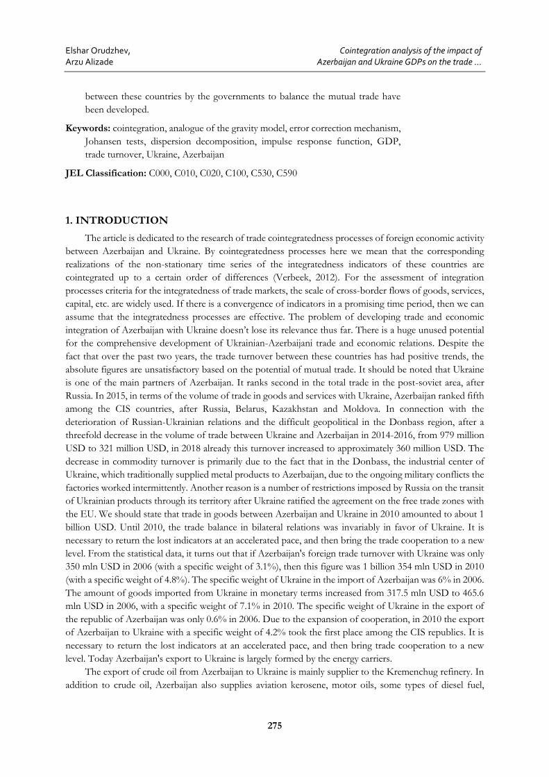
The Multiple Regression Model estimated by the Least Squares method, built by using the Eviews

package, is presented in Table 2.

Таble 2

Estimated multiple regression model with logarithms of variables

Dependent Variable: LNUKRТ

Method: Least Squares

Date:14.07.20 Time: 15:17

Sample:1994 – 2018 Included observations: 25

Variable Coefficient Std. Error t-Statistic Prob.

LNGDPAZ 0.139474 0.135355 1.030433 0.3145

LNGDPUKR 1.413870 0.308301 4.586001 0.0002

LNRESİDS 0.011772 0.055296 0.212883 0.8335

C -15.52129 3.799718 -4.084854 0.0005

R-squared 0.904768 Mean dependent var 12.50237

Adjusted R-squared 0.891163 S.D. dependent var 1.057384

S.E. of regression 0.348835 Akaike info criterion 0.877210

Sum squared resid 2.555401 Schwarz criterion 1.072230

Log likelihood -6.965128 Hannan-Quinn criter. 0.931301

F-statistic 66.50474 Durbin-Watson stat 1.530174

Prob(F-statistic) 0.000000


Open/ As Equation / Estimate Equation Method LS – Least Squares (NLS and ARMA)

and has the following formal form:

LNUKRТ = 0.13947443961*LNGDPAZ+ 1.4138696781*LNGDPUKR +

0.011771574448*LNRESİDS - 15.5212948644 (3)

The estimates obtained confirm the theoretical assumptions regarding the signs of the coefficients for

the GDP variables of both states. In accordance with the hypothesis Put forward,the coefficient for direct

transportation costs turned out to be negative, i.e. The power of d, which we have taken equal to -2. As

shown from the results obtained in Table 2, for the general formal model is the most accurate, the coefficient

of determination turned out to be high 90%.

Let's review other predictive characteristics of the model based on CUSUM tests. These tests are based

on calculating the accumulated sums of recursive residuals and accumulated sums of squares of recursive



281

residuals and evaluating the corresponding equations. The test results are diagrams of the dynamics of these

values and 95% confidence intervals for them. If the recursive estimates of the residuals go beyond the

critical boundaries, then this indicates the instability of the model parameters. Test results for model (3) are

described in Graph 2 and 3. The location of the blue line between the red lines in Graph 2 means that the

hypothesis Н0- about the stability of the parameters is accepted, and if the blue line intersects with the red

ones, then the hypothesis Н0__is rejected in favor of the alternative hypothesis, На - about the instability of

the parameters relative to the length of the time interval. Graph 3 shows that recursive estimates of residuals

(CUSUM) and squares of recursive estimates of residuals (CUSUM of Squares) do not go beyond 95%

confidence intervals, which once again confirms the high predictive capabilities of the developed model (3).

Thus, the prognostic tests carried out showed that model (3) is stable, correctly specified, and has stable

prognostic characteristics.

Graph 2. Recursive residual estimates Graph 3. Standardized residual estimates

Source: The results of procedures realized Source: The results of procedures realized in EViews 8 software package in

EViews 8 software package View /Stability diagnostics/Recursive View/Actual, Fitted, Residual /Standardized

Estimates (OLS test)/CUSUM test residuals

Let us pay attention to the correlation coefficients between the factors represented by the correlation

matrix of Table 3:

Тable 3

Correlation matrix

LNUKRT LNGDPAZ LNGDPUKR

LNUKR T 1.000000 0.887882 0.948657

LNGDPAZ 0.887882 1.000000 0.905568

LNGDPUKR 0.948657 0.905568 1.000000


As Group/View / Covariance analyses/Correlation

A qualitative assessment of the tightness of the relationship between factors is revealed on the

Chaddock scale. Based on this scale, if the value of an element of this matrix is between 0.5 and 0.7, then

the tightness of the relationship between the corresponding factors is considered noticeable, and if the value

of the element is in the range (0.7; 0.9), then the tightness of the relationship of the respective pairs is

accepted as high.

To check the significance of the constructed model (3), the observed and critical values of the Fisher

criterion are calculated. These values are respectively equal to 66.5 and 3.44 at the significance level of 5%

and degrees of freedom 𝑘1 = 2, 𝑘2 = 22к2 = 21. Due to the fact 66.5 >3.44, the model according to this

criterion is considered significant. Estimation of coefficients for LNGDPAZ and LNRESIDS according to

t-statistics at a significance level of 0.05 can be considered insignificant.

-15

-10

-5

0

5

10

15

98 00 02 04 06 08 10 12 14 16 18

CUSUM 5% Significance

-2.0

-1.5

-1.0

-0.5

0.0

0.5

1.0

1.5

2.0

94 96 98 00 02 04 06 08 10 12 14 16 18

Standardized Residuals


Vol.14, No.3, 2021

282

The autocorrelation was verified by using Darbin-Watson d-statistics. From the table of critical values

of d-statistics for the number of observations 25, the number of explanatory variables 2 and the given

significance level of 0.05, the values of 𝑑𝑙𝑜𝑤 = 1,21 и 𝑑𝑢𝑝 = 1,55, which divide interval [0,4] into five

areas, found the observed value 𝑑𝑜𝑏𝑠𝑒𝑟 = 1,53. 𝑑набл = 1,08. As 1,21 < 𝑑𝑜𝑏𝑠𝑒𝑟 =1,53< 1,55. The

observed value has an uncertainty value, nothing can be said about the presence of autocorrelations using

the Durbin-Watson test.

Now we consider the problem of the presence of heteroscedasticity. Heteroscedasticity leads to the

fact that estimates of the regression coefficients aren’t effective, and variances of the distributions of the

coefficient estimates increase. The heteroscedasticity of the residuals was verified by White test and the

results are presented in Table 4.

The value 𝑛𝑅2 = 𝑂𝑏𝑠 ∗ 𝑅 − 𝑠𝑞𝑢𝑎𝑟𝑒𝑑,where 𝑛 = 25, 𝑅2- the coefficient of determination for the

auxiliary regression of the squares of residuals for all repressors, their squares, pair wise products and a

constant, equal 5.563891, and this value almost coincides with the 𝜒0,352 (5) =5,563807. The corresponding

P-value is greater than 0.05, i.e. the null hypothesis about the homoscedasticity of the random term needn’t

be rejected.

Table 4

Results of White test for heteroscedasticity

F-statistics 1.087810 Probability F (5,19) 0.3988

Obs* determination coefficient 5.563891 Prob. Chi-Square (5) 0.3510


View /Residual diagnostics/Hetroskedasticity test/White test

The stationarity of the time series of the modeling variables was verified by using the advanced Dickey-

Fuller Test. Testing results showed that the initial series and their first differences aren’t stationary, and

second-order difference operators are stationary. The test results are provided in Table 5.

Table 5

Result of dickey-fuller test

Variables Statistic Criteria

Critical value 1%

Critical value 5%

Critical value 10%

Prob.

Second differences

LNUKRT -8.159048 -4.440739 -3.632896 -3.254671 0.0000

LNGDPUKR -5.371924 -4.440739 -3.632896 -3.254671 0.0014

LNGDPAZ -4.615559 -4.440739 -3.632896 -3.254671 0.0070

LNRESIDS -4.881168 -4.532598 -3.673616 -3.277364 0.0051

Source: The results of procedures realized in EViews 8 software package View /Unit root test/Augmented

Dickey – Fuller/2nd difference/Intercept and trend, m=1,2,3,4,5 lags

The verification of the causal relationships between the factors for lag values m = 1, 2, 3, 4 was carried

out through the Granger Test. The Granger Causality Test, with the exception of one directions, confirmed

the presence of a two-way causal relationship, which indicates the existence of a third variable, which is the

real cause of the change in the two considered variables. Only for lag m = 4, the causal relationships between

ΔLNGDPAZ and ΔLNUKRT is opposite. Here, Δ denotes the difference operator of the corresponding

variable.

Previously we have created a formal model with a trend component. The coefficient of determination

approximately coincides with this coefficient of the model (1). However, other statistics are low-meaning.

Therefore, we keep the initial model (1).



283

The results of the above tests appear that the estimates of the regression coefficients are poor. The

reason for this is the nonstationarity of the studied series. Engle-Granger and Johansen's cointegration

approach is the correct mathematical description of the series. This approach can be applied to create an

error correction model if the time series included in the model are nonstationary but integratedness of the

same order. To check cointegration, we should analyze the need to include a constant or a constant and

linear trend in the model and check the model's adequacy using Student's t-tests, Fisher's, and other statistics.

We will accept possible variants of 5 hypotheses to apply the appropriate test procedures 𝐻2(𝑟), 𝐻1∗(𝑟),

𝐻1(𝑟), 𝐻∗(𝑟), 𝐻(𝑟)– the data don’t have a deterministic trend, the cointegration equation contains neither

a trend nor a free term; 𝐻1∗(𝑟) – the data don’t have a deterministic trend, the cointegration relation contains

a free term and doesn’t contain a trend; 𝐻1(𝑟) – the data contains a deterministic trend, the cointegration

equation contains a free term and doesn’t contain a trend; 𝐻∗(𝑟) – the data have a deterministic linear trend,

the cointegration relation has both a trend and a free term; 𝐻(𝑟) – the data contain a deterministic quadratic

trend, cointegration equation contains a trend and a free term.

The Engle-Granger and Johansen testing results are presented in Tables 6, 6.1 and 6.2:

Table 6

Results of tests of Engle-Granger and Johansen for cointegration by logarithms of variables

Date 14/07/20 Time: 17:35

Sample: 1994-2018

Included observations: 20

Series: ΔLNUKRT ΔLNGDPAZ ΔLNGDPUKR

Selected (0.01 level*) Number of Cointegrating Relations by Model

Data Trend:

None None Linear Linear Quadratic

Test Type

𝐻2(𝑟) 𝐻1∗(𝑟) 𝐻1(𝑟) 𝐻∗(𝑟) 𝐻(𝑟)

Trace 3 2 3 1 3

Max-Eig

3 1 3 1 1

Information Criteria by Rank and Model

Data Trend:

None None Linear Linear Quadratic

Rank or No. of CEs

𝐻2(𝑟) 𝐻1∗(𝑟) 𝐻1(𝑟) 𝐻∗(𝑟) 𝐻(𝑟)

Log Likelihood by Rank (rows) and Model (columns)

0 -24.24897 -24.24897 -24.20618 -24.20618 -23.99838

1 -2.270148 -2.172438 -2.135090 -2.117768 -2.054350

2 7.508518 7.663538 7.668070 7.691298 7.754099

3 13.10042 13.30656 13.30656 13.33109 13.33109

Akaike Information Criteria by Rank (rows) and Model (columns)

0 3.324897 3.324897 3.620618 3.620618 3.899838

1 1.727015 1.817244 2.013509 2.111777 2.305435

2 1.349148* 1.533646 1.633193 1.830870 1.924590

3 1.389958 1.669344 1.669344 1.966891 1.966891

Schwarz Information Criteria by Rank (rows) and Model (columns

0 3.772977 3.772977 4.218058 4.218058 4.646637

1 2.473814 2.613830 2.909668 3.057722 3.350954

2 2.394667* 2.678738 2.828072 3.125322 3.268829

3 2.734197 3.162942 3.162942 3.609849 3.609849


View /Cointegration test/Johansen system cointegration test /Summarize all 5 sets assumption


Vol.14, No.3, 2021

284

Тable 6.1

Result test of Max-Eigenvalue

Hypothesis Alternative

hypothesis

Max-Eigenvalue

statistics

Critical value

1%

Prob.

𝐻0:r=0* 𝐻𝐴:r >0 44.17683 30.83396 0.0001

𝐻0:r=1 𝐻𝐴:r >1 19.61813 23.97534 0.0463

𝐻0:r=2 𝐻𝐴:r >2 11.27959 16.55386 0.0798


View /Cointegration test/Johansen system cointegration test /İntercept and trend in CE

Таble 6.2

Result of Trace test

Hypothesis Alternative

hypothesis

Trace statistics Critical value

1%

Prob.

𝐻0:r=0* 𝐻𝐴:r >0 75.07456 49.36275 0.0000

𝐻0:r=1 𝐻𝐴:r >1 30.89772 31.15385 0.0109

𝐻0:r=2 𝐻𝐴:r >2 11.27959 16.55386 0.0798


View /Cointegration test/Johansen system cointegration test /İntercept and trend in CE

The results of the Trace, Max-Eigenvalue tests are the same only for the 𝐻∗(𝑟) variant from table 6.

In the case of 𝐻∗(𝑟) the information criteria of Akaike and Schwarz have low values of 1.830870 and

3.057722, respectively. The last two tables shown the number of cointegration vectors in the series of

dynamics, we first tested the null hypothesis that there are no cointegration vectors, i.e. r = 0, there is one

such vector against the alternative hypothesis. We rejected the null hypothesis, since the calculated values

were more than the critical values, from where we came to the conclusion that there is one vector of

cointegration. Then we tested the hypothesis, there is one vector against the alternative hypothesis that there

are two cointegration vectors. Here, we accepted the null hypothesis because calculated criteria are less than

the critical values. The same is true in the case of the alternative hypothesis of three and four vectors. Thus,

we concluded that there is one vector of cointegration.

The Engle-Granger and Johansen Tests showed that all variables are cointegratedness, which confirms

their long-term relationship and the authenticity of the correlation. Given the informational criteria of

Akaike and Schwartz, it was found out that the best one was the lag equal to 2. One cointegration relation

is obtained with the degree of integration of the second order and the cointegration rank equal to 1.

According to (Verbeek, 2012), the system of integratedness order 2 and cointegratedness series can be

represented in the form of a vector error correction model (VECM) with a lag of 2 and a rank of 1, which

expresses the long-term equilibrium relationship of variables and authenticity. Their correlation, which

makes it possible to measure deviations from equilibrium in the event of shocks and the speed of its

recovery. The following error correction equation was found for the second order differences of the

logarithmic values of Azerbaijan's GDP by following procedures of the Eviews program,

Δ (Δ LNUKRТ) = 0.0355603015521*( Δ LNUKRТ (-1) - 3.1870061501* Δ LNGDPAZ (-1) -

2.39804627923* Δ LNGDPUKR (-1) + 0.831686150061* Δ LNRESIDS (-1) - 0.202025767492 ) -

1.12183480279* Δ (Δ LNUKRT (-1)) - 0.265731742651* Δ (Δ LNUKRT (-2)) - 1.91013865615* Δ (Δ

LNGDPAZ (-1)) - 2.66911616438* Δ (Δ LNGDPAZ (-2)) + 0.68045831886* Δ (Δ LNGDPUKR (-1)) +

0.443920173228* Δ (Δ LNGDPUKR (-2)) + 0.0179318911639* Δ (Δ LNRESIDS (-1)) +

+0.0349766890005* Δ (Δ LNRESIDS (-2)) + 0.0751422282878 (4)



285

Where ∆(∙) = ∆𝑡(∙); ∆(−𝑖) = ∆𝑡−𝑖(∙), 𝑡 = 1,3, "∙" the corresponding variable is indicated.

When we implementing the Granger causality test, we showed that there are feedbacks between

variables. It is easy to obtain error correction models for the remaining variables by using Eviews software

procedures, following similar procedures:

Δ(Δ LNGDPAZ )= 0.129695443071*( Δ LNUKRT (-1) - 3.1870061501* Δ (Δ LNGDPAZ (-1) -

2.39804627923* Δ LNGDPUKR (-1) + 0.831686150061* Δ LNRESIDS (-1) - 0.202025767492 ) -

0.141834541652* Δ (Δ LNUKRT (-1)) - 0.0833088402909* Δ (Δ LNUKRT (-2)) - 0.441538690404* Δ (Δ

LNGDPAZ (-1)) - 0.755478401528* Δ (Δ LNGDPAZ (-2)) + 0.3237492508* Δ (Δ LNGDPUKR (-1)) +

0.34419371965* Δ (Δ LNGDPUKR (-2)) - 0.0774495416136* Δ (Δ LNRESIDS (-1)) - 0.0234505524657*

* Δ (Δ LNRESIDS (-2)) + 0.0371313594229 (5)

Δ (ΔLNGDPUKR) = 0.281005895234*( (-1) - 3.1870061501* Δ LNGDPAZ (-1) - 2.39804627923*

Δ LNGDPUKR (-1) + 0.831686150061* Δ LNRESIDS (-1) - 0.202025767492 ) - 0.285248125451* Δ (Δ

LNUKRT (-1)) - 0.148058177738* Δ (Δ LNUKRТ (-2)) + 0.143862237724* Δ (Δ LNGDPAZ (-1)) +

0.230600836987* Δ (Δ LNGDPAZ (-2)) + 0.105303313039* Δ (Δ LNGDPUKR) (-1)) - 0.1312986001*

Δ(Δ LNGDPUKR (-2)) - 0.187035333378* Δ (Δ LNRESIDS (-1)) - 0.0791985748849*

* Δ (Δ LNRESIDS (-2)) + 0.059546588866 (6)

Model (4), (5), (6) are statistically correct, since the previous stages of construction ensure that its

variables are stationary.

The adequacy of the constructed error model (4), (5), (6) is estimated based on the results of the general

analysis of residuals (errors) of the three regression equations. LM (VAR Residual Serial Correlation LM

Test) - testing the hypothesis of serial correlations; Jarque-Bera test using of the joint normal distribution

of random errors; White heteroscedasticity test: No Cross Terms - about the constancy of the dispersion of

the residuals. Equivalent forms of criteria were used for make a decision, which are a comparison of the

conditions for the significance of ε and P-values that are indicated in the columns of Prob. in the evaluation

window of the test tables 7,8,9.

Table 7

VAR Residual Serial Correlation LM Test

Null hypothesis: no consistent correlation with lag h

Date: 14.07.20 Time: 18:26

Sample: 1994

2018

Included observations: 21

Lags LM-Stat Probability

1 9.099665 0.4281

2 9.692784 0.3759


Var/View/Residual tests/ Auto correlation LM


Vol.14, No.3, 2021

286

Table 8

VAR Residual Normality Test

Orthogonalization: Khaletsky (Lutkepohl)

Null hypothesis: residuals are multidimensional normally

Date: 14/07/20 Time : 19:45

Sample: 1994 2018

Included observations:21

Components Skewness Chi-square df Probability

1 -0.323396 0.366047 1 0.5452

2 -0.640859 1.437450 1 0.2306

3 0.088869 0.027642 1 0.8680

Joint 1.831139 3 0.6082

Components Kurtosis Chi-square df Probability

1 2.582207 0.152732 1 0.6959

2 3.743534 0.483738 1 0.4867

3 2.959332 0.001447 1 0.9697

Joint 0.637917 3 0.8877

Components Jarque-Bera df Probability

1 0.518779 2 0.7715

2 1.921188 2 0.3827

3 0.029089 2 0.9856

Joint 2.469056 6 0.8719


Var/View/Residual tests/Normality test

Table 9

White test for heteroscedasticity: No Cross Terms

Date: 14/07/20 Time: 20:15

Sample: 1994 2018

Included observations:21

Joint test:

Chi-square df Probability

75.69128 72 0.3602

Dependent Determination

coefficient

F(12,8) Probability Chi-square

(12)

Probability

res1*res1 0.895876 5.735936 0.0096 18.81339 0.0931

res2*res2 0.230033 0.199171 0.9935 4.830694 0.9634

res3*res3 0.176262 0.142652 0.9985 3.701503 0.9882

res2*res1 0.588175 0.952146 0.5469 12.35168 0.4179

res3*res1 0.499298 0.664798 0.7475 10.48526 0.5735

res3*res2 0.232051 0.201447 0.9932 4.873076 0.9621


Var/View/Residual tests/ White test for heteroscedasticity: No Cross Terms

Table 8 shows that skewness is close to zero (-0.640859) and kurtosis is close to three (3.743534),

which better smoothes out the empirical distribution of the residuals of the deviation from the normal,

rather than the corresponding values (-1.674268) and (5.268172) from table 1.



287

We can conclude that the null hypotheses based on the results of estimations of tables 7, 8, 9: about

the mutual independence of the residuals; the normal joint distribution of random errors; on the constancy

of the variance of errors at the 5% level do not deviate and the constructed system of error models (4), (5),

(6) are adequate.

For a fully informative study, in addition to the Granger causality test, it’s necessary to analyze the

response of impulse functions. These functions represent a median estimate with 90% confidence interval

of the endogenous variable for the positive shock of one standard deviation of the exogenous variable and

shows the time of return to the equilibrium trajectory. The confidence intervals were obtained by

bootstrapping with 100 replications, as described in (Hall, 1992). The test results for 10 year time horizons

are described in Graph 4:

Graph 4. Reactions of impulse response functions


Var/View/impulse response/table and MS Excel 2010 insert /Charts group/Line with Markers

Graph 4 shows that the response of the variables to a deviation from the general stochastic trend isn’t

the same. In response to shocks, the endogenous variable travels its part of the path to equilibrium.

To study the influence of exogenous variables on the endogenous variable according to data for the

last 10 years, an econometric method of decomposition of the variances of forecast errors is used, which

-0,6

-0,4

-0,2

0

0,2

0,4

0,6

1 2 3 4 5 6 7 8 9 10

Perc

en

tag

e d

evi

ati

on

fro

mtr

en

d

Response ΔLNUKRT

Years

[1]

[2] [3]

[1]-ΔLNUKRT[2]-ΔLNGDPUK[3]-ΔLNGDPAZ

-0,1

-0,05

0

0,05

0,1

0,15

0,2

1 2 3 4 5 6 7 8 9 10

Pers

an

tag

e d

evi

ati

on

fro

m

tren

d

Response ΔLNGDPAZ

Years

[3]

[1]

[2]

[1]-ΔLNUKRT[2]-ΔLNGDPUKR[3]-ΔLNGDPAZ

-0,1

-0,05

0

0,05

0,1

0,15

0,2

1 2 3 4 5 6 7 8 9 10

Pers

en

tag

e d

evi

ati

on

fro

mtr

en

d

Response ΔLNGDPUKR

[1]-ΔLNUKRT[2]-ΔLNGDPUK[3]-ΔLNGDPAZ[2]

[3]

[1]

Years


Vol.14, No.3, 2021

288

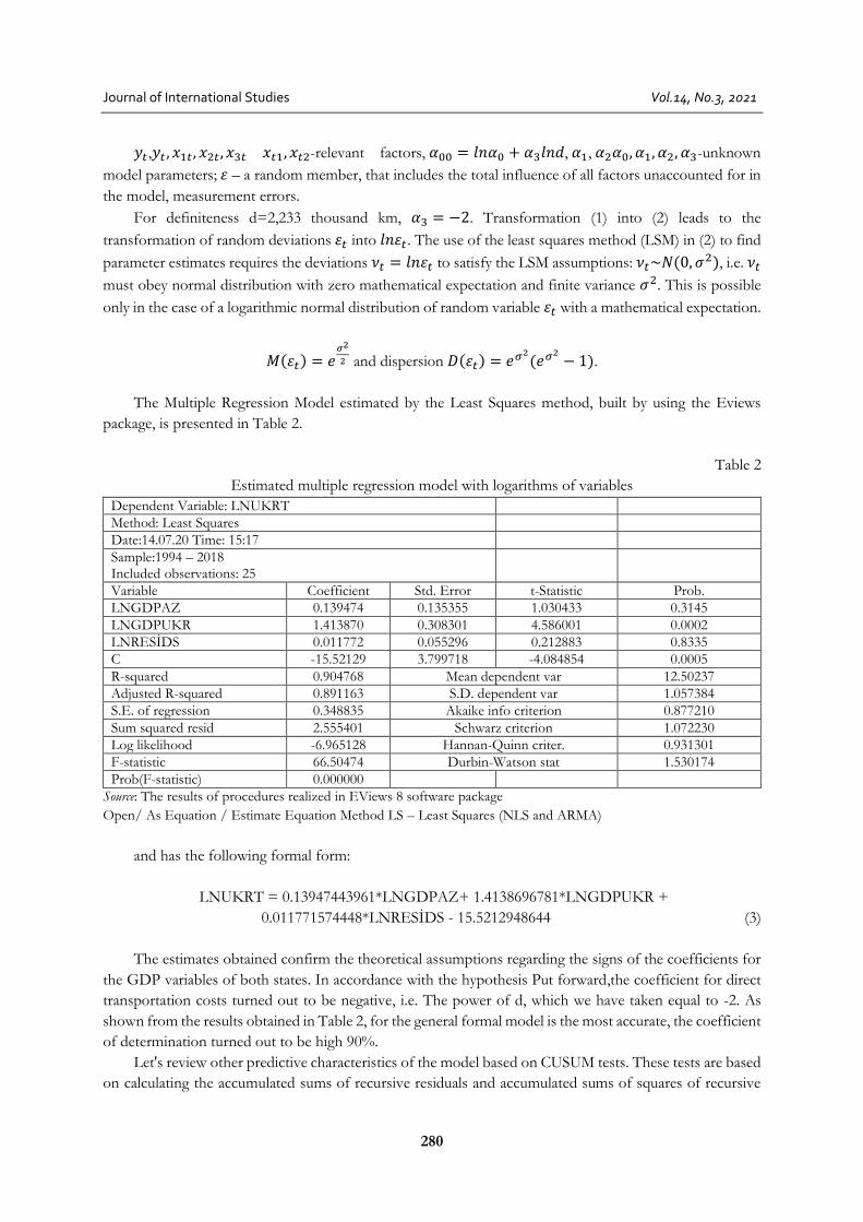
determines the contribution of changes in this variable to the own variance of the forecast. errors and

variance of other variables. The verification results of the relevant tests are shown in Graph 5:

Graph 5. Decompositions of forecast error variances


Var/View/Variance decompasitions /table and MS Excel 2010 insert /Charts group/Line with Markers

0

20

40

60

80

100

1 2 3 4 5 6 7 8 9 10

Deco

mp

osi

tio

n o

f d

isp

ers

ion

Δ

LN

UK

RT

(%)

[1]

[2]

[3] Years


0

20

40

60

80

100

1 2 3 4 5 6 7 8 9 10

Deco

mp

osi

tio

n o

f d

isp

ers

ion

Δ

LN

GD

PU

KR

(%)


[2]

[1]

[3]

Years

0

20

40

60

80

100

1 2 3 4 5 6 7 8 9 10

Deco

mp

osi

tio

n o

f d

isp

ers

ion

ΔL

NG

DP

AZ

(%)


[3]

[2]

[1] Years

[1]-ΔLNУКРТ



289

5. CONCLUSIONS

The conducted cointegration analysis of the mutual influence of the GDPs Azerbaijan and country’s

trade with Ukraine allows us to formulate a number of conclusions:

1. The results of the lagged dependencies show that the constructed cointegration relations formed

from the difference operators of the second order of the effective logarithm values of the initial variables,

can be considered significant. The inclusion in models (4), (5), (6) of the parameters of auto-regression and

a moving average of the second order has an economic interpretation that the foreign trade between Ukraine

and Azerbaijan is significantly influenced by the states themselves, trying to bring the foreign trade balance

as close as possible to the possible minimum, therefore, during each year, volumes of the foreign trade

between these countries are adjusted depending on the values in previous periods.

2. The constructed vector model of error correction with two components allows us to evaluate the

quantitative characteristics of the short-term and long-term dynamics of the relationship between the

studied indicators. In particular, estimates of lag parameters are provided and the speeds of convergence to

the equilibrium trajectory are determined. Deviations from equilibrium trajectories in previous time periods

are restored in subsequent time periods.

3. The long-term equilibrium relationship is stable in that, if broken in the short-term periods, it is

restored. Combining the statistical long-term and dynamic short-term relationships between the variables in

one line, we can measure the deviations from the equilibrium in the event of shocks and the rate of its

recovery by using relations (5) and (6).

4. The contributions to the variance of forecast errors of changes in the own dispersion of the effective

factor and variance of the causal factor is determined.

5. The trade simulation using the above methodology allows forecasting trade flows. The introduction

of tools for studying the dynamics of the causality of the GDP of both countries of the trade turnover

between them on the basis of the proposed method for monitoring unsteady time series will allow us to

determine the strategy of stabilization of export-import operations, the real state of the trade relations in

the current period and to obtain adequate forecasts for the development of economic cooperation in the

future. The estimates obtained from correction mechanisms (4), (5), (6) make it possible to carry out

dynamic analyses for effective government regulation of export-import operations between the two

countries to balance the trade and improve corresponding inclusive parameters of long-term sustainable

economic growth of these states. It is very important for the respective foreign trade regulatory bodies of

both countries to conduct monitoring using methodology of the system of vector error correction model

(4), (5), (6). It is enough carry out monitoring on an annual basis after the release of official information on

the results of the reporting year.

REFERENCES

Andronova, I.V. (2012). Evolution of integration processes in the post-Soviet space. Bulletin of RUDN University, Series

Economics, 5, 72-81.

Chebotareva N.N., & Fayzulina, Yu. V. (2016). Analysis of export and import of goods and services in Ukraine. Network

journal "Scientific Result". Series "Economic Research", 2, 1(7),.57-63.

Dankevych, V.Y., Pyvovar, P.V., & Dankevych, Y.M. (2020). The impact of World Trade Liberalization on the

Development of Domestic Brewing Companies. The Problems of economy, 1(43), 59-67.

Frolov, S.M., & Savytska, О.І. (2016). Research of Causal Relations between Components of foreign Trade and

Economic Performance of the Region Country and World. The Problems of economy, 1, 282-288.

Golovan, D.V. (2012). Dynamics of the structure of foreign trade and the international strategy of economic

development of Ukraine. Economy and management of machinery and equipment enterprises: problems of theory and practice,

3(19), 98-205.


Vol.14, No.3, 2021

290

Hall, P. (1992). On Bootstrap Confidence Intervals in Nonparametric Regression. Annals of Statistics 20(2), 695-711.

Johnson, R. R. (2015). A Guide to Using Eviews with Using Econometrics: A Practical Guide University of San Diego.

Kalyuzhna, N. G. (2020). International Trade Integration of Ukraine in the context of Deepening Interstate Conflict.

The Problems of economy 1(43), 27-35.

Kharlamova, G., & Vertelieva, O. (2013). The International Competitiveness of Countries: Economic-Mathematical

Approach, Economics & Sociology, 6(2), 39-52.

Kenneth, N. B., & Carey, P. (2010). Data Analysis with Microsoft Excel: Updated for Office 2007, Third Edition, p. 613,

ISBN-13: 978-0-495-39178-4, Cengage Learning products are represented in Canada by Nelson Education,

Ltd.

Moroz, S., Nagyova, L., Bilan, Yu., Horska, E., & Polakova, Z. (2017). The current state and prospects pf trade relations

between Ukraine and the European Union: The Visegard vector Economic Annals-XXI, 163(1-2(1)), 14-21.

Orudzhev E.G., & Huseynova S.M. (2019). The cointegration relations between Azerbaijan’s GDP and the balances

of the trade relations of Russia and Belarus. Journal of Contemporary Applied Mathematics, 9(2), 73-92.

Orudzhev, E. G., & Huseynova, S. M. (2020). About one cointegration issue of trade relations Azerbaijan, Russia,

Belarus. Journal of Advanced Research in Dynamical and Control Systems (JARDCS), 12(6), 1385-1394.

Orudzhev, E.G., & Alizade, A.R. (2020). Cointegration of Trade and Economic Relations between Azerbaijan and

Ukraine. Journal of Contemporary Applied Mathematics, 2, 83-97. http://journalcam.com/wp-

content/uploads/2020/05/100110.pdf

Pylin, A.G. (2015). Foreign economic relations of Azerbaijan in the context of regional integration. Problems of the post-

Soviet space https://www.postsovietarea.com/jour

Tinbergen, J. (1962). An Analysis of World Trade Flows. // Shaping the World Economy. Suggestions for an International

Economic Policy. Appendix VI. – New-York: The Twentieth Century Fund, 262-293.

Verbeek, M. (2012). A Guide to Modern Econometrics. John Wiley & Sons p. 386

www.stat.gov.az (08.07.2020)

www.worldbank.com (08.07.2020)

Documents

Cointegration analysis of the impact of Azerbaijan and