Cohomology of the adjoint of Hopf algebras · 2020-01-09 · Cohomology of the adjoint of Hopf algebras 21 (A) (B) S Figure 3: Conditions for the YBE for Hopf algebras Rad : H ⊗

Journal of Generalized Lie Theory and Applications Vol. 2 (2008), No. 1, 19–34

Cohomology of the adjoint of Hopf algebras

J. Scott CARTER a, Alissa S. CRANS b, Mohamed ELHAMDADI c, and Masahico SAITO c

a University of South Alabama, Mobile, AL 36688, USAEmail: [email protected]

b Loyola Marymount Unversity, Los Angeles, CA 90045, USAE-mail: [email protected]

c University of South Florida, Tampa, FL 33620, USAE-mails: [email protected] and [email protected]

Abstract

A cohomology theory of the adjoint of Hopf algebras, via deformations, is presented bymeans of diagrammatic techniques. Explicit calculations are provided in the cases of groupalgebras, function algebras on groups, and the bosonization of the super line. As applications,solutions to the YBE are given and quandle cocycles are constructed from groupoid cocycles.

1 Introduction

Algebraic deformation theory [10] can be used to define 2-dimensional cohomology in a widevariety of contexts. This theory has also been understood diagrammatically [7, 16, 17] viaPROPs, for example. In this paper, we use diagrammatic techniques to define a cohomologicaldeformation of the adjoint map ad(x ⊗ y) =

∑S(y(1))xy(2) in an arbitrary Hopf algebra. We

have concentrated on the diagrammatic versions here because diagrammatics have led to topo-logical invariants [6, 13, 19], diagrammatic methodology is prevalent in understanding particleinteractions and scattering in the physics literature, and most importantly kinesthetic intuitioncan be used to prove algebraic identities.

The starting point for this calculation is a pair of identities that the adjoint map satisfies andthat are sufficient to construct Woronowicz’s solution [22] R = (1 ⊗ ad)(τ ⊗ 1)(1 ⊗ ∆) to theYang-Baxter equation (YBE): (R⊗1)(1⊗R)(R⊗1) = (1⊗R)(R⊗1)(1⊗R). We use deformationtheory to define an extension 2-cocycle. Then we show that the resulting 2-coboundary map,when composed with the Hochschild 1-coboundary map is trivial. A 3-coboundary is definedvia the “movie move” technology. Applications of this cohomology theory include constructingnew solutions to the YBE by deformations and constructing quandle cocycles from groupoidcocycles that arise from this theory.

The paper is organized as follows. Section 2 reviews the definition of Hopf algebras, de-fines the adjoint map, and illustrates Woronowicz’s solution to the YBE. Section 3 contains thedeformation theory. Section 4 defines the chain groups and differentials in general. Examplecalculations in the case of a group algebra, the function algebra on a group, and a calculation ofthe 1- and 2-dimensional cohomology of the bosonization of the superline are presented in Sec-tion 5. Interestingly, the group algebra and the function algebra on a group are cohomologicallydifferent. Moreover, the conditions that result when a function on the group algebra satisfiesthe cocycle condition coincide with the definition of groupoid cohomology. This relationship isgiven in Section 6, along with a construction of quandle 3-cocycles from groupoid 3-cocycles. InSection 7, we use the deformation cocycles to construct solutions to the Yang-Baxter equation.

20 J. S. Carter, A. S. Crans, M. Elhamdadi, and M. Saito

2 Preliminaries

We begin by recalling the operations and axioms in Hopf algebras, and their diagrammaticconventions depicted in Figures 1 and 2.

A coalgebra is a vector space C over a field k together with a comultiplication ∆ : C → C⊗Cthat is bilinear and coassociative: (∆ ⊗ 1)∆ = (1 ⊗∆)∆. A coalgebra is cocommutative if thecomultiplication satisfies τ∆ = ∆, where τ : C⊗C → C⊗C is the transposition τ(x⊗y) = y⊗x.A coalgebra with counit is a coalgebra with a linear map called the counit ε : C → k such that(ε⊗ 1)∆ = 1 = (1⊗ ε)∆ via k⊗C ∼= C. A bialgebra is an algebra A over a field k together witha linear map called the unit η : k → A, satisfying η(a) = a1 where 1 ∈ A is the multiplicativeidentity and with an associative multiplication µ : A⊗A→ A that is also a coalgebra such thatthe comultiplication ∆ is an algebra homomorphism. A Hopf algebra is a bialgebra C togetherwith a map called the antipode S : C → C such that µ(S ⊗ 1)∆ = ηε = µ(1 ⊗ S)∆, where ε isthe counit.

In diagrams, the compositions of maps are depicted from bottom to top. Thus a multiplicationµ is represented by a trivalent vertex with two bottom edges representing A ⊗ A and one topedge representing A. Other maps in the definition are depicted in Fig. 1 and axioms are depictedin Fig. 2.

x

∆

x x(1) (2)

ε

η

xS( )

x x y

τ

xy

TranspositionComultiplicationMultiplication Unit Counit Antipode

x y

µ

xy

S

Figure 1: Operations in Hopf algebras

Associativity

Unit Counit Counit is an algebra hom

CompatibilityCoassociativity

Antipode conditionUnit is a coalgebra hom

S S

Figure 2: Axioms of Hopf algebras

Let H be a Hopf algebra. The adjoint map Ady : H → H for any y ∈ H is defined byAdy(x) = S(y(1))xy(2), where we use the common notation ∆(x) = x(1)⊗x(2) and µ(x⊗y) = xy.Its diagram is depicted in Fig. 3 (A). Notice the analogy with group conjugation: in a groupring H = kG over a field k, where ∆(y) = y ⊗ y and S(y) = y−1, we have Ady(x) = y−1xy. Forthe adjoint map ad : H ⊗H → H we have ad(x⊗ y) = Ady(x).

Definition 1. Let H be a Hopf algebra and ad be the adjoint map. Then the linear map

Cohomology of the adjoint of Hopf algebras 21

(A) (B)

S

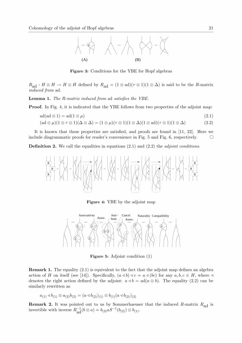
Figure 3: Conditions for the YBE for Hopf algebras

Rad : H ⊗ H → H ⊗ H defined by Rad = (1 ⊗ ad)(τ ⊗ 1)(1 ⊗ ∆) is said to be the R-matrixinduced from ad.

Lemma 1. The R-matrix induced from ad satisfies the YBE.

Proof. In Fig. 4, it is indicated that the YBE follows from two properties of the adjoint map:

ad(ad⊗ 1) = ad(1⊗ µ) (2.1)(ad⊗ µ)(1⊗ τ ⊗ 1)(∆⊗∆) = (1⊗ µ)(τ ⊗ 1)(1⊗∆)(1⊗ ad)(τ ⊗ 1)(1⊗∆) (2.2)

It is known that these properties are satisfied, and proofs are found in [11, 22]. Here weinclude diagrammatic proofs for reader’s convenience in Fig. 5 and Fig. 6, respectively.

Definition 2. We call the equalities in equations (2.1) and (2.2) the adjoint conditions.

R

R

R

R

R

R

Figure 4: YBE by the adjoint map

CompatibilityAssociativityAssoc.

CancelAssoc.

NaturalityAnti−hom.

S

SS

S

S

S

S

S

SS

Figure 5: Adjoint condition (1)

Remark 1. The equality (2.1) is equivalent to the fact that the adjoint map defines an algebraaction of H on itself (see [14]). Specifically, (a / b) / c = a / (bc) for any a, b, c ∈ H, where /denotes the right action defined by the adjoint: a / b = ad(a ⊗ b). The equality (2.2) can besimilarly rewritten as

a(1) / b(1) ⊗ a(2)b(2) = (a / b(2))(1) ⊗ b(1)(a / b(2))(2)

Remark 2. It was pointed out to us by Sommerhaeuser that the induced R-matrix Rad isinvertible with inverse R−1

ad(b⊗ a) = b(3)aS−1(b(2))⊗ b(1).


Def.

Counit

UnitDef.

antip.

compat.

Redraw

Counit

Unit

co-assoc.

assoc.assoc.

co-assoc.co-assoc.

antipode

compatiblity

assoc.

NaturalityCo-assoc.

S

S

S

S

S

S

SS

S

S S

S

S

S

S

S

S

Figure 6: Adjoint condition (2)

3 Deformations of the adjoint map

We follow the exposition in [16] for deformation of bialgebras to propose a similar deformationtheory for the adjoint map. In light of Lemma 1, we deform the two equalities (2.1) and (2.2).Let H be a Hopf algebra and ad its adjoint map.

Definition 3. A deformation of (H, ad) is a pair (Ht, adt) where Ht is a k[[t]]-Hopf algebra givenby Ht = H ⊗ k[[t]] with all Hopf algebra structures inherited by extending those on Ht withthe identity on the k[[t]] factor (the trivial deformation as a Hopf algebra), with a deformationsof ad given by adt = ad + tad1 + · · · + tnadn + · · · : Ht ⊗Ht → Ht, where adi : H ⊗H → H,i = 1, 2, · · · , are maps.

Suppose ad = ad+ · · ·+ tnadn satisfies the adjoint conditions (equalities (2.1) and (2.2)) modtn+1, and suppose that there exist adn+1 : H ⊗H → H such that ad + tn+1adn+1 satisfies theadjoint conditions mod tn+2. Define ξ1 ∈ Hom(H⊗3,H) and ξ2 ∈ Hom(H⊗2,H⊗2) by

ad(ad⊗ 1)− ad(1⊗ µ) = tn+1ξ1 mod tn+2

(ad⊗µ)(1⊗τ⊗1)(∆⊗∆)−(1⊗µ)(τ⊗1)(1⊗∆)(1⊗ad)(τ⊗1)(1⊗∆) = tn+1ξ2 mod tn+2

For the first adjoint condition (2.1) of ad + tn+1adn+1 mod tn+2 we obtain

((ad + tn+1adn+1)⊗ 1)− (ad + tn+1adn+1)(1⊗ µ) = 0 mod tn+2

which is equivalent by degree calculations to

ad(adn+1 ⊗ 1) + adn+1(ad⊗ 1)− adn+1(1⊗ µ) = ξ1

For the second adjoint condition (2.2) of ad + tn+1adn+1 mod tn+2 we obtain

((ad + tn+1adn+1)⊗ µ)(1⊗ τ ⊗ 1)(∆⊗∆)

−(1⊗ µ)(τ ⊗ 1)(1⊗∆)(1⊗ (ad + tn+1adn+1))(τ ⊗ 1)(1⊗∆) = 0 mod tn+2

which is equivalent by degree calculations to

(adn+1 ⊗ µ)(1⊗ τ ⊗ 1)(∆⊗∆)− (1⊗ µ)(τ ⊗ 1)(1⊗∆)(1⊗ adn+1)(τ ⊗ 1)(1⊗∆) = ξ2

In summary we proved the following.

Lemma 2. The map ad + tn+1adn+1 satisfies the adjoint conditions mod tn+2 if and only if

ad(adn+1 ⊗ 1) + adn+1(ad⊗ 1)− adn+1(1⊗ µ) = ξ1

(adn+1 ⊗ µ)(1⊗ τ ⊗ 1)(∆⊗∆)− (1⊗ µ)(τ ⊗ 1)(1⊗∆)(1⊗ adn+1)(τ ⊗ 1)(1⊗∆) = ξ2

We interpret this lemma as (ξ1, ξ2) being the primary obstructions to formal deformationof the adjoint map. In the next section we will define coboundary operators, and show that(ξ1, ξ2) = (0, 0) gives that adn+1 is a 2-cocycle, and that (ξ1, ξ2) satisfies the 3-cocycle condition,just as in the case of deformations and Hochshild cohomology for bialgebras.


4 Differentials and cohomology

4.1 Chain groups

We define chain groups, for positive integers n, n > 1, and i = 1, . . . , n by

Cn,iad (H;H) = Hom(H⊗(n+1−i),H⊗i), Cn

ad(H;H) = ⊕i>0, i≤n+1−i Cn,iad (H;H)

Specifically, chain groups in low dimensions of our concern are:

C2ad(H;H) = Hom(H⊗2,H), C3

ad(H;H) = Hom(H⊗3,H)⊕Hom(H⊗2,H⊗2)

For n = 1, define

C1ad(H;H) = {f ∈ Homk(H,H) | fµ = µ(f⊗1)+µ(1⊗f), ∆f = (f⊗1)∆+(1⊗f)∆} (4.1)

In the remaining sections we will define differentials that are homomorphisms between the chaingroups:

dn,i : Cnad(H;H) → Cn+1,i

ad (H;H)(= Hom(H⊗(n+2−i),H⊗i))

that will be defined individually for n = 1, 2, 3 and for i with 2i ≤ n+ 1, and

D1 = d1,1 : C1ad(H;H) → C2

ad(H;H), D2 = d2,1 + d2,2 : C2ad(H;H) → C3

ad(H;H)

D3 = d3,1 + d3,2 + d3,3 : C3ad(H;H) → C3

ad(H;H)

4.2 First differentials

By analogy with the differential for multiplication, we make the following definition.

Definition 4. The first differential d1,1 : C1ad(H;H) → C2,1

ad (H;H) is defined by

d1,1(f) = ad(1⊗ f)− fad + ad(f ⊗ 1)

Diagrammatically, we represent d1,1 as depicted in Fig. 7, where a 1-cochain is representedby a circle on a string.

( d 1,1 )

Figure 7: The 1-differential

,2,2 ( )( )d 2,1 0η

1 0, d

Figure 8: A diagram for a 2-cochain and the 2-cocycle conditions

4.3 Second differentials

Definition 5. Define the second differentials by d2,1

ad(φ) = ad(φ⊗ 1) +φ(ad⊗ 1)−φ(1⊗µ) and

d2,2

ad(φ) = (φ⊗ µ)(1⊗ τ ⊗ 1)(∆⊗∆)− (1⊗ µ)(τ ⊗ 1)(1⊗∆)(1⊗ φ)(τ ⊗ 1)(1⊗∆)

Diagrams for 2-cochain and 2-differentials are depicted in Fig. 8.

Theorem 1. D2D1 = 0.

Proof. This follows from direct calculations, and can be seen from diagrams in Figs. 9 and10.


if0( d 2,1 )

Figure 9: The 2-cocycle condition for a 2-coboundary, Part I

if

d 2,2 ( )

0

Figure 10: The 2-cocycle condition for a 2-coboundary, Part II

4.4 Third differentials

Definition 6. We define 3-differentials as follows. Let ξi ∈ C3,i(H;H) for i = 1, 2. Then

d3,1

ad(ξ1, ξ2) = ad(ξ1 ⊗ 1) + ξ1(1⊗ µ⊗ 1)− ξ1(ad⊗ 12 + 12 ⊗ µ)

d3,2

ad(ξ1, ξ2) = (ad⊗ µ)(1⊗ τ ⊗ 1)(12 ⊗∆)(ξ2 ⊗ 1) + (1⊗ µ)(τ ⊗ 1)(1⊗ ξ2)(Rad ⊗ 1)

+ (1⊗ µ)(12 ⊗ µ)(τ ⊗ 12)(1⊗ τ ⊗ 1)(12 ⊗∆)((12 ⊗ ξ1)

· (1⊗ τ ⊗ 12)(τ ⊗ 13)(12 ⊗ τ ⊗ 1)(1⊗∆⊗∆))

− (ξ1 ⊗ µ)(12 ⊗ τ ⊗ 1)(12 ⊗ µ⊗ 12)(1⊗ τ ⊗ 13)(∆⊗∆⊗∆)− ξ2(1⊗ µ)

d3,3

ad(ξ1, ξ2) = (1⊗ µ⊗ 1)(τ ⊗ 12)(1⊗∆⊗ 1)(1⊗ ξ2)(τ ⊗ 1)(1⊗∆)

+ (ξ2 ⊗ µ)(1⊗ τ ⊗ 1)(∆⊗∆)− (1⊗∆)ξ2

Diagrams for 3-cochains are depicted in Fig. 11. See Fig. 12 (A), (B), and (C) for thediagrammatics for d3,1, d3,2 and d3,3, respectively.

Theorem 2. D3D2 = 0.

Proof. The proof follows from direct calculations that are indicated in Figs. 13, 14 and 15. Wedemonstrate how to recover algebraic calculations from these diagrams for the part(d3,3d2,2)(η1) = 0 for any η1 ∈ C2(H;H). This is indicated in Fig. 15, where subscripts ad aresuppressed for simplicity. Let ξ2 = d2,2(η1) ∈ C3,2(H;H) (note that ξ1 = d2,1(η1) ∈ C3,1(H;H)does not land in the domain of d3,3). The first line of Fig. 15 represents the definition of the

1ξ ξ 2

Figure 11: Diagrams for 3-cochains


(C)(A) (B)

Figure 12: The 3-differentials

differential

d3,3

ad(ξ1, ξ2) = (1⊗ µ⊗ 1)(τ ⊗ 12)(1⊗∆⊗ 1)(1⊗ ξ2)(τ ⊗ 1)(1⊗∆)

+ (ξ2 ⊗ µ)(1⊗ τ ⊗ 1)(∆⊗∆)− (1⊗∆)ξ2

where each term represents each connected diagram. The first parenthesis of the second linerepresents that

ξ2 = d2,2(η1) = (η1 ⊗ µ)(1⊗ τ ⊗ 1)(∆⊗∆)− (1⊗ µ)(τ ⊗ 1)(1⊗∆)(1⊗ η1)(τ ⊗ 1)(1⊗∆)

is substituted in the first term (1⊗µ⊗ 1)(τ ⊗ 12)(1⊗∆⊗ 1)(1⊗ ξ2)(τ ⊗ 1)(1⊗∆). When thesetwo maps are applied to a general element x⊗ y ∈ H ⊗H, the results are computed as

η1(x(1) ⊗ y(2)(1))(1) ⊗ y(1)η1(x(1) ⊗ y(2)(1))(2) ⊗ x(2)y(2)(2)

−η1(x⊗ y(2)(2))(1)(1) ⊗ y(1)η1(x⊗ y(2)(2))(1)(2) ⊗ y(2)(1)η1(x⊗ y(2)(2))(2)

By coassociativity applied to y and η1(x⊗ y(2)(2)), the second term is equal to

η1(x⊗ y(2))(1) ⊗ y(1)(1)η1(x⊗ y(2))(2)(1) ⊗ y(1)(2)η1(x⊗ y(2))(2)(2)

which is equal, by compatibility, to η1(x⊗y(2))(1)⊗(y(1)η1(x⊗y(2))(2))(1)⊗(y(1)η1(x⊗y(2))(2))(2).This last term is represented exactly by the last term in the second line of Fig. 15, and thereforeis cancelled. The map represented by the second term in the second line of Fig. 15 cancels withthe third term by coassociativity, and the fourth term cancels with the sixth by coassociativityapplied twice and compatibility once. Other cases (Figs. 13, 14) are computed similarly.

From point of view of Lemma 2, we state the relation between deformations and the thirddifferential map as follows.

Corollary 1. The primary obstructions (ξ1, ξ2) to formal deformations in Lemma 2 representa 3-cocycle: D3(ξ1, ξ2) = 0.

Furthermore, in Lemma 2 we see thatD2(adn+1) = (ξ1, ξ2), so we regard that the obstructionsrepresent a cohomology class [ξ1, ξ2] ∈ H3(H;H) after the definition of the cohomology groupsin the next section.


4.5 Cohomology groups

For convenience define C0(H;H) = 0, D0 = 0 : C0(H;H) → C1(H;H).Then Theorems 1 and 2 are summarized as follows.

Theorem 3. C = (Cn, Dn)n=0,1,2,3 is a chain complex.

This enables us to propose

Definition 7. The adjoint n-coboundary, cocycle and cohomology groups are defined by:

Bn(H;H) = Im(Dn−1), Zn(H;H) = Ker(Dn), Hn(H;H) = Zn(H;H)/Bn(H;H)

for n = 1, 2, 3.

3,1d

Figure 13: d3,1(d2,1) = 0

Figure 14: d3,2(d2,1, d2,2) = 0

Figure 15: d3,3(d2,2) = 0

5 Examples

5.1 Group algebras

Let G be a group and H = kG be its group algebra with the coefficient field k (char k 6= 2).Then H has a Hopf algebra structure induced from the group operation as multiplication,∆(x) = x ⊗ x for basis elements x ∈ G, and the antipode induced from S(x) = x−1 for x ∈ G.Here and below, we denote the conjugation action on a group G by x / y := y−1xy. Note thatthis defines a quandle structure on G; see [12].


Lemma 3. C1ad(kG; kG) = 0.

Proof. For any given w ∈ G write f(w) =∑

u∈G au(w)u, where a : G→ k is a function. Recallthe defining equality (4.1). The LHS of the second condition is written as

∆f(w) = ∆

(∑u

au(w)u

)=

∑u

au(w)u⊗ u

and the RHS is written as

((f ⊗1)∆+(1⊗f)∆)(w) = ((f ⊗1)+(1⊗f))(w⊗w) =∑

h

ah(w)(h⊗w)+∑

v

av(w)(w⊗v)

For a given w, fix u and then compare the coefficients of u⊗u. In the LHS we have au(w), whileon the RHS w = u, and furthermore w = h = v for u ⊗ u. Thus the diagonal coefficient mustsatisfy aw(w) = aw(w) + aw(w), so that aw(w) = 0 since char k 6= 2. In the case w 6= u, neitherterm of h⊗ w nor w ⊗ v is equal to u⊗ u, hence au(w) = 0.

Lemma 4. For x, y ∈ G, write φ(x, y) =∑

u au(x, y)u, where a : G×G→ k. Then the inducedlinear map φ : kG⊗ kG→ kG is in Z2

ad(kG; kG) if and only if a satisfies

ax/y(x, y) + a(x/y)/z(xC y, z)− a(x/y)/z(x, yz) = 0

for any x, y, z ∈ G.

Proof. The first 2-cocycle condition for φ : kG⊗ kG→ kG is written by

z−1φ(x⊗ y)z + φ(y−1xy ⊗ z)− φ(x⊗ yz) = 0

for basis elements x, y, z ∈ G. The second is formulated by

LHS = φ(x⊗ y)⊗ xy =∑

u

au(x, y)(u⊗ xy), RHS =∑w

aw(x, y)(w ⊗ yw)

They have the common term u⊗xy for w = y−1xy = u, and otherwise they are different terms.Thus we obtain aw(x, y) = 0 unless w = y−1xy. For these terms, the first condition becomes

z−1(ay−1xy(x, y)y−1xy)z+az−1y−1xyz(y

−1xy, z)z−1y−1xyz−az−1y−1xyz(x, yz)z−1y−1xyz = 0

and the result follows.

Remark 3. In the preceding proof, since the term aw(x, y) = 0 unless w = x/y, let ax/y(x, y) =a(x, y). Then the condition stated becomes a(x, y) + a(x / y, z)− a(x, yz) = 0.

Proposition 1. Let G be a group. Let (ξ1, ξ2) ∈ C3ad(kG; kG), where ξ1 is the map that is

defined by linearly extending ξ1(x ⊗ y ⊗ z) =∑

u∈G cu(x, y, z)u. Then (ξ1, ξ2) ∈ Z3ad(kG; kG)

if and only if ξ2 = 0 and the coefficients satisfy the following properties: (a) cu(x, y, z) = 0 ifu 6= z−1y−1xyz, and (b) c(x, y, z) = cz−1y−1xyz(x, y, z) satisfies

c(x, y, z) + c(x, yz, w) = c(y−1xy, z, w) + c(x, y, zw)

Proof. Suppose (ξ1, ξ2) ∈ Z3ad(kG; kG). Let ξ2 be the map that is defined by linearly extending

ξ2(x⊗ y) =∑

u,v∈G au,v(x, y)u⊗ v. Then the third 3-cocycle condition from Definition 6 gives:(abbreviating au,v(x, y) = au,v)

d3,3(ξ1, ξ2)(x⊗ y) =∑u1,v1

au1,v1(u1 ⊗ yu1 ⊗ v1) +∑u2,v2

au2,v2(u2 ⊗ v2 ⊗ xy)


−∑u3,v3

au3,v3(u3 ⊗ v3 ⊗ v3) = 0

We first consider terms in which the third tensorand is xy. From the third summand, this forcesthe second tensorand to be xy, so we collect the terms of the form (u⊗ xy ⊗ xy). This gives

∑u

(au,xy + au,xy − au,xy)(u⊗ xy ⊗ xy) = 0

which implies au,xy = 0 for all u ∈ G. The remaining terms are∑

u1,v1 6=xy

au1,v1(u1⊗ yu1⊗ v1)+∑

u2,v2 6=xy

au2,v2(u2⊗ v2⊗xy)−∑

u3,v3 6=xy

au3,v3(u3⊗ v3⊗ v3) = 0

From the second sum we obtain au,v(x, y) = 0 for v 6= xy. In conclusion, if d3,3(ξ1, ξ2) = 0 forkG then ξ2 = 0.

We now consider d3,2(ξ1, ξ2), with ξ2 = 0. Let ξ1 be the map that is defined by linearlyextending ξ1(x ⊗ y ⊗ z) =

∑u∈G cu(x, y, z)u for x, y, z ∈ G. The second 3-cocycle condition

from Definition 6, with ξ2 = 0, is∑

u cuu ⊗ yzu =∑

v cvv ⊗ xyz. In order to combine liketerms, we need yzu = xyz, meaning u = z−1y−1xyz. Thus, cu(x, y, z) = 0 except in the casewhen u = z−1y−1xyz. In this case, we obtain ξ1(x⊗ y ⊗ z) = c(x, y, z)z−1y−1xyz ⊗ xyz, wherec(x, y, z) = cz−1y−1xyz(x, y, z).

Finally we consider the first 3-cocycle condition from Definition 6, which is formulated forbasis elements by

w−1 ξ1(x⊗ y ⊗ z) w + ξ1(x⊗ yz ⊗ w) = ξ1(x / y ⊗ z ⊗ w) + ξ1(x⊗ y ⊗ zw)

Substituting in the formula for c(x, y, z) which we found above, we obtain

c(x, y, z) + c(x, yz, w) = c(y−1xy, z, w) + c(x, y, zw)

This is a group 3-cocycle condition with the first term x · c(y, z, w) omitted. This is expectedfrom Fig. 12 (A). Constant functions, for example, satisfy this condition.

Next we look at a coboundary condition. A 3-coboundary is written as

ξ1(x⊗y⊗z) =∑

u

cu(x, y, z)u = d2,1(φ)(x⊗y⊗z) = z−1φ(x⊗y)z+φ(y−1xy⊗z)−φ(x⊗yz)

If we write φ(x, y) =∑

u

hu(x, y)u, then

(d2,1(φ))(x⊗ y ⊗ z) = z−1

(∑u

hu(x, y)u

)z +

(∑v

hv(y−1xy, z)v

)−

(∑w

hw(x, yz)w

)

=∑

g

( hzgz−1(x, y) + hg(y−1xy, z)− hg(x, yz))g

Hence

cu(x, y, z) = hzuz−1(x, y) + hu(y−1xy, z)− hu(x, yz)

and in particular for the coefficients cu(x, y, z) from Proposition 1,

c(x, y, z) = cz−1y−1xyz(x, y, z) = hy−1xy(x, y) + hz−1y−1xyz(y−1xy, z)− hz−1y−1xyz(x, yz)

By setting hy−1xy(x, y) = a(x, y), we obtain


Lemma 5. A 3-cocycle c(x, y, z) is a coboundary if for some a(x, y),

c(x, y, z) = a(x, y) + a(y−1xy, z)− a(x, yz)

Remark 4. From Remark 3, Proposition 1, and Lemma 5, we have the following situation. The2-cocycle condition, the 3-cocycle condition, and the 3-coboundary condition, respectively, givesrise to the equations

a(x, y) + a(y−1xy, z)− a(x, yz) = 0

c(x, y, z) + c(x, yz, w)− c(y−1xy, z, w)− c(x, y, zw) = 0


This suggests a cohomology theory, which we investigate in Section 6.

Proposition 2. For the symmetric group G = S3 on three letters, we have H1ad(kG; kG) = 0

and H2ad(kG; kG) ∼=

⊕

3

(kG) for k = C and F3.

Proof. By Lemma 3, we have H1ad(kG; kG) = 0 and B2

ad(kG, kG) = 0. Hence H2(kG; kG) ∼=Z2

ad(kG; kG), which is computed by solving the system of equations stated in Lemma 4 andRemark 3. Computations by Maple and Mathematica shows that the solution set is of dimension3 and generated by (a((1 2 3), (1 2)), a((2 3), (1 3 2)), and a((1 3), (1 2)) for the above mentionedcoefficient fields.

5.2 Function algebras on groups

Let G be a finite group and k a field with char(k) 6= 2. The set kG of functions from G to kwith pointwise addition and multiplication is a unital associative algebra. It has a Hopf algebrastructure using kG×G ∼= kG ⊗ kG with comultiplication defined through ∆ : kG → kG×G by∆(f)(u⊗ v) = f(uv) and the antipode by S(f)(x) = f(x−1).

Now kG has basis (the characteristic function) δg : G→ k defined by δg(x) = 1 if x = g andzero otherwise. Since S(δg) = δg−1 and ∆(δh) =

∑uv=h δu ⊗ δv, the adjoint map becomes

ad(δg ⊗ δh) =∑

uv=h

δu−1δgδv ={δg if h = 10 otherwise

Lemma 6. C1ad(kG; kG) = 0.

Proof. Recall the defining equality (4.1). Let G = {g1, . . . , gn} be a given finite group andabbreviate δgi = δi for i = 1, . . . , n. Describe f : kG → kG by f(δi) =

∑nj=1 s

ji δj . Then

fµ = µ(f ⊗ 1) + µ(1⊗ f) is written for basis elements by LHS = f(δiδj) and

RHS = f(δi)δj + δif(δj) = (n∑

`=1

s`iδ`)δj + δi(

n∑

h=1

shj δh) = sj

i δj + sijδi

For i = j we obtain LHS =∑n

w=1 swi δw and RHS = 2si

iδi so that sji = 0 for all i, j as desired.

Lemma 7. Z2ad(kG; kG) = 0.

Proof. Recall that d2,1(η1) = ad(η1⊗1)+η1(ad⊗1)−η1(1⊗µ) for η1 ∈ C2ad(kG, kG). Describe

a general element η1 ∈ C2ad(kG, kG) by η1(δi ⊗ δj) =

∑` s

`i jδ`. Consider d2,1(η1)(δa ⊗ δb ⊗ δc).

If c 6= 1, then the first term is zero by the definition of ad. If c 6= 1 and b = 1, then the thirdterm is also zero, and we obtain that the second term η1(δa ⊗ δc) is zero. Hence η1(δa ⊗ δc) = 0unless c = 1. Next, set b = c = 1 in the general form. Then all three terms equal η1(δa ⊗ δ1)and we obtain η1(δa ⊗ δ1) = 0, and the result follows.


By combining the above lemmas, we obtain the following

Theorem 4. For any finite group G and a field k, we have Hnad(kG; kG) = 0 for n = 1, 2.

Observe that k(G) and kG are cohomologically distinct.

5.3 Bosonization of the superline

Let H be generated by 1, g, x with relations x2 = 0, g2 = 1, xg = −gx and Hopf algebrastructure ∆(x) = x ⊗ 1 + g ⊗ x, ∆(g) = g ⊗ g, ε(x) = 0, ε(g) = 1, S(x) = −gx, S(g) = g (thisHopf algebra is called the bosonization of the superline [15], page 39, Example 2.1.7).

The operation ad is represented by the following table, where, for example, ad(g ⊗ x) = 2x.

1 g x gx

1 1 1 0 0g g g 2x 2xx x −x 0 0gx gx −gx 0 0

Remark 5. The induced R-matrix Rad has determinant 1, the characteristic polynomial is(λ2 + 1)2(λ+ 1)4(λ− 1)8, and the minimal polynomial is (λ2 + 1)(λ+ 1)(λ− 1)2.

Proposition 3. The first cohomology of H is given by H1ad(H,H) ∼= k.

Proof. Recall the defining equality (4.1). Let f ∈ C1ad(H;H). Assume that f(x) = a + bx +

cg + dxg and f(g) = α+ βx+ γg + δxg where a, b, c, d, α, β, γ, δ ∈ k. Applying f to both sidesof the equation g2 = 1, one obtains α = γ = 0. Similarly evaluating both sides of the equation∆f = (f ⊗ 1)∆ + (1 ⊗ f)∆ at g gives β = δ = 0, one obtains that f(g) = 0. In a similar way,applying f to the equations x2 = 0 and xg = −gx gives rise to, respectively, a = 0 and c = 0.Also evaluating ∆f = (f ⊗ 1)∆+(1⊗ f)∆ at x gives rise to d = 0. We also have f(x) = f(xg)g(since g2 = 1),which implies f(xg) = bxg. In conclusion f satisfies f(1) = 0 = f(g), f(x) = bx,and f(xg) = b(xg). Now consider f in the kernel of D1, that is f satisfies

d1,1(f) = ad(1⊗ f)− fad + ad(f ⊗ 1)

It is directly checked on all the generators u⊗ v of H ⊗H that d1,1(f)(u⊗ v) = 0. This impliesthat H1(H,H) ∼= k.

Proposition 4. For any field k of characteristic not 2, H2ad(H,H) ∼= k3.

Proof. With d1,1 = 0 from the preceding Proposition, we haveH2ad(H,H) ∼= Z2

ad(H,H). Eitherthe direct hand calculations from definitions or the computer calculations give the followinggeneral solution for the 2-cocycle φ(a⊗ b) represented in the following table:

1 g x gx

1 0 0 0 0g 0 0 α1 α1x 0 −α1 0 0gx 0 γg β1 + γx −β1 + γx

Here, for example, φ(gx⊗ g) = γg, where α, β, γ are free variables.


6 Adjoint, groupoid, and quandle cohomology theories

From Remark 4, the adjoint cohomology leads us to cohomology, especially for conjugategroupoids of groups as defined below. Through the relation between Reidemeister moves forknots and the adjoint, groupoid cohomology, we obtain a new construction of quandle cocycles.In this section we investigate these relations. First we formulate a general definition. Manyformulations of groupoid cohomology can be found in literature, and relations of the followingformulation to previously known theories are not clear. See [20], for example.

Let G be a groupoid with objects Ob(G) and morphisms G(x, y) for x, y ∈ Ob(G). Letfi ∈ G(xi, xi+1), 0 ≤ i < n, for non-negative integers i and n. Let Cn(G) be the free abeliangroup generated by {(x0, f0, . . . , fn) | x0 ∈ Ob(G), fi ∈ G(xi, xi+1), 0 ≤ i < n}. The boundarymap ∂ : Cn+1(G) → Cn(G) is defined by by linearly extending

∂(x0, f0, . . . , fn) = (x1, f1, . . . , fn) +n−1∑

i=0

(−1)i+1(x0, f0, . . . , fi−1, fifi+1, fi+2, . . . , fn)

+ (−1)n+1(x0, f0 . . . , fn−1)

Then it is easily seen that this differential defines a chain complex. The corresponding groupoid1- and 2-cocycle conditions are written as

a(x1, f1)− a(x0, f0f1) + a(x0, f0) = 0c(x1, f1, f2)− c(x0, f0f1, f2) + c(x0, f0, f1f2)− c(x0, f0, f1) = 0

The general cohomological theory of homomorphisms and extensions applies, such as:

Remark 6. Let G be a groupoid and A be an abelian group regarded as a one-object groupoid.Then α : hom(x0, x1) → A gives a groupoid homomorphism from G to A, which sends Ob(G) tothe single object of A, if and only if a : C1(G) → A, defined by a(x0, f0) = α(f0), is a groupoid1-cocycle. Next we consider extensions of groupoids. Define

◦ : (hom(x0, x1)×A)× (hom(x1, x2)×A) → hom(x0, x2)×A

by (f0, a) ◦ (f1, b) = (f0f1, a+ b+ c(x0, f0, f1)), where c(x0, f0, f1) ∈ hom(C2(G), A). If G ×A isa groupoid, the function c with the value c(x0, f0, f1) is a groupoid 2-cocycle.

Example. Let G be a group. Define the conjugate groupoid of G, denoted G, by Ob(G) = Gand Mor(G) = G × G, where the source of the morphism (x, y) ∈ hom(x, y−1xy) is x and itstarget is y−1xy, for x, y ∈ G. Composition is defined by (x, y) ◦ (y−1xy, z) = (x, yz). For thisexample, the groupoid 1- and 2-cocycle conditions are

a(x, y) + a(y−1xy, z)− a(x, yz) = 0

c(x, y, z) + c(x, yz, w)− c(y−1xy, z, w)− c(x, y, zw) = 0

Diagrammatic representations of these equations are depicted in Fig. 16 (A) and (B), respec-tively. Furthermore, c is a coboundary if


Compare with Remark 4.For G = S3, the symmetric group on 3 letters, with coefficient group C, Z2, Z3, Z5 and Z7,

respectively, the dimensions of the conjugation groupoid 2-cocycles are 3, 5, 4, 3 and 3.


(B)1y xy

yzx

yz

wzw

yz1y xy

1y xyc( , z, w)

x

yz

w

x

yz

zw

c(x, y, zw)w

c(x, y, z) c(x, yz, w)

1y xy

yz

1y xy

yzx

y

z

1y xya( , z)

x

y

z x

a(x, y) a(x, yz)

(A)

Figure 16: Diagrams for groupoid 1- and 2-cocycles

For the rest of the section, we present new constructions of quandle cocycles from groupoidcocycles of conjugate groupoids of groups. Let G be a finite group, and a : G2 → k be adjoint2-cocycle coefficients that were defined in Remark 3. These satisfy

a(x, y) + a(x / y, z)− a(x, yz) = 0

Proposition 5. Let ψ(x, y) = a(x, y). Then ψ satisfies the rack 2-cocycle condition

ψ(x, y) + ψ(x / y, z) = ψ(x, z) + ψ(x / z, y / z)

Proof. By definition

ψ(x, y) + ψ(x / y, z) = a(x, yz)

ψ(x, z) + ψ(x / z, y / z) = a(x, z) + a(z−1xz, z−1yz) = a(x, z(y / z))

Let G be a finite group, and c : G3 → k be a coefficient of the adjoint 3-cocycle defined inProposition 1. This satisfies

c(x, y, z) + c(x, yz, w) = c(x / y, z, w) + c(x, y, zw)

Proposition 6. Let G be a group that is considered as a quandle under conjugation. Thenθ : G3 → k defined by

θ(x, y, z) = c(x, y, z)− c(x, z, z−1yz)

is a rack 3-cocycle.

Proof. We must show that θ satsifies

θ(x, y, z) + θ(x / z, y / z, w) + θ(x, z, w) = θ(x / y, z, w) + θ(x, y, w) + θ(x / w, y / w, z / w)

We compute

LHS− RHS = [c(x, y, z)− c(x, z, z−1yz)]

+ [c(z−1xz, z−1yz, w)− c(z−1xz,w,w−1z−1yzw)] + [c(x, z, w)− c(x,w,w−1zw)]

− [c(y−1xy, z, w)− c(y−1xy,w,w−1zw) ]− [c(x, y, w)− c(x,w,w−1yw)]

− [c(w−1xw,w−1yw,w−1zw)− c(w−1xw,w−1zw,w−1z−1yzw)]

= [ c(x, y, z)− c(y−1xy, z, w) ]− [c(x, z, z−1yz)− c(z−1xz, z−1yz, w)]

+ [c(x, z, w)− c(z−1xz,w,w−1z−1yzw)]

− [c(x,w,w−1zw)− c(w−1xw,w−1zw,w−1z−1yzw)]

− [c(x, y, w)− c(y−1xy,w,w−1zw)] + [c(x,w,w−1yw)− c(w−1xw,w−1yw,w−1zw)]

= [−c(x, yz, w) + c(x, y, zw)]− [−c(x, zz−1yz, w) + c(x, z, z−1yzw)]

+ [−c(x, zw,w−1z−1yzw) + c(x, z, ww−1z−1yzw)] + c(x,w,w−1yww−1zw] = 0


7 Deformations of R-matrices by adjoint 2-cocycles

In this section we give, in an explicit form, deformations of R-matrices by 2-cocycles of theadjoint cohomology theory we developed in this paper. Let H be a Hopf algebra and ad itsadjoint map. In Section 3 a deformation of (H, ad) was defined to be a pair (Ht, adt) whereHt is a k[[t]]-Hopf algebra given by Ht = H ⊗ k[[t]] with all Hopf algebra structures inheritedby extending those on Ht. Let A = (H ⊗ k[[t]])/(t2)) and the Hopf algebra structure mapsµ,∆, ε, η, S be inherited on A. As a vector space A can be regarded as H ⊕ tH

Recall that a solution to the YBE, R-matrix Rad is induced from the adjoint map. Thenfrom the constructions of the adjoint cohomology from the point of view of the deformationtheory, we obtain the following deformation of this R-matrix induced from the adjoint map.

Theorem 5. Let φ ∈ Z2ad(H;H) be an adjoint 2-cocycle. Then the map R : A ⊗ A → A ⊗ A

defined by R = Rad+tφ satisfies the YBE.

Proof. The equalities of Lemma 2 hold in the quotient A = (H ⊗ k[[t]])/(t2), where n = 1 andthe modulus t2 is considered. These cocycle conditions, on the other hand, were formulatedfrom the motivation from Lemma 1 for the induced R-matrix Rad to satisfy the YBE. Hencethese two lemmas imply the theorem.

Example. In Subsection 5.3, the adjoint map ad was computed for the bosonization H of thesuperline, with basis {1, g, x, gx}, as well as a general 2-cocycle φ with three free variables α, β, γwritten by

φ(g ⊗ x) = φ(g ⊗ gx) = α1, φ(x⊗ g) = −α1, φ(gx⊗ g) = γg

φ(gx⊗ x) = β1 + γx, φ(gx⊗ gx) = −β1 + γx

and zero otherwise. Thus we obtain the deformed solution to the YBE R = Rad+tφ on A withthree variables tα, tβ, tγ of degree one.

8 Concluding remarks

In [7] we concluded with A Compendium of Questions regarding our discoveries. Here we attemptto address some of these questions by providing relationships between this paper and [7], andoffer further questions for our future consideration.

It was pointed out in [7] that there was a clear distinction between the Hopf algebra caseand the cocommutative coalgebra case as to why self-adjoint maps satisfy the YBE. In [7] acohomology theory was constructed for the coalgebra case. In this paper, many of the same ideasand techniques, in particular deformations and diagrams, were used to construct a cohomologytheory in the Hopf algebra case, with applications to the YBE and quandle cohomology.

The aspects that unify these two theories are deformations and a systematic process wecall “diagrammatic infiltration.” So far, these techniques have only been successful in defin-ing coboundaries up through dimension 3. This is a deficit of the diagrammatic approach, butdiagrams give direct applications to other algebraic problems such as the YBE and quandle coho-mology, and suggest further applications to knot theory. By taking the trace as in Turaev’s [21],for example, a new deformed version of a given invariant is expected to be obtained.

Many questions remain: Can 3-cocycles be used for solving the tetrahedral equation? Canthey be used for knotted surface invariants? Can the coboundary maps be expressed skeintheoretically? How are the deformations of R-matrices related to deformations of underlyingHopf algebras? When a Hopf algebra contains a coalgebra, such as the universal envelopingalgebra and its Lie algebra together with the ground field of degree-zero part, what is therelation between the two theories developed in this paper and in [7]? How these theories, otherthan the same diagrammatic techniques, can be uniformly formulated, and to higher dimensions?


Acknowledgements

JSC (NSF Grant DMS #0301095, #0603926) and MS (NSF Grant DMS #0301089, #0603876)gratefully acknowledge the support of the NSF without which substantial portions of the workwould not have been possible. The opinions expressed in this paper do not reflect the opinions ofthe National Science Foundation or the Federal Government. JSC, ME, and MS have benefitedfrom several detailed presentations on deformation theory that have been given by Jorg Feldvoss.AC acknowledges useful and on-going conversations with John Baez.

References

[1] N. Andruskiewitsch and M. Grana. From racks to pointed Hopf algebras. Adv. Math. 178 (2003),177–243.

[2] J. C. Baez and A. S. Crans. Higher-Dimensional Algebra VI: Lie 2-Algebras. Theory Appl. Categ.12 (2004), 492–538.

[3] J. C. Baez and L. Langford. 2-tangles. Lett. Math. Phys. 43 (1998), 187–197.[4] E. Brieskorn. Automorphic sets and singularities. In ”Proc. AMS-IMS-SIAM Joint Summer Research

Conference in Mathematical Sciences on Artin’s Braid Group held at the University of California,Santa Cruz, California, July 13–26, 1986. J. S. Birman and A. Libgober, Eds. AMS, Providence, RI,1988.“. Contemp. Math., 78 (1988), 45–115.

[5] J. S. Carter, M. Elhamdadi, and M. Saito Twisted Quandle homology theory and cocycle knotinvariants Algebr. Geom. Topol. 2 (2002), 95–135.

[6] J. S. Carter, D. Jelsovsky, S. Kamada, L. Langford, and M. Saito. Quandle cohomology and state-sum invariants of knotted curves and surfaces. Trans. Amer. Math. Soc. 355 (2003), 3947–3989.

[7] J. S. Carter, A. Crans, M. Elhamdadi, and S. Saito. Cohomology of Categorical Self-Distributivity.To appear in Journal of Homotopy Theory and Related Structures; preprint math. GT/0607417.

[8] A. S. Crans. Lie 2-algebras. Ph.D. Dissertation, 2004, UC Riverside. Preprint math.QA/0409602.[9] R. Fenn and C. Rourke. Racks and links in codimension two. J. Knot Theory Ramifications, 1

(1992), 343–406.[10] M. Gerstenharber and S. D. Schack. Bialgebra cohomology, deformations, and quantum groups.

Proc. Nat. Acad. Sci. U.S.A. 87 (1990), 478–481.[11] M. A. Hennings. On solutions to the braid equation identified by Woronowicz. Lett. Math. Phys.

27 (1993), 13–17.[12] D. Joyce. A classifying invariant of knots, the knot quandle. J. Pure Appl. Algebra, 23 (1982) 37–65.[13] G. Kuperberg. Involutory Hopf algebras and 3-manifold invariants. Int. J. Math. 2 (1991), 41–66.[14] S. Majid. A Quantum Groups Primer. London Math. Soc. Lecture Note Ser. 292. Cambridge Univ.

Press, Cambridge, 2002.[15] S. Majid. Foundations of Quantum Group Theory. Cambridge Univ. Press, Cambridge, 1995.[16] M. Markl and J. D. Stasheff. Deformation theory via deviations. J. Algebra, 170 (1994), 122–155.[17] M. Markl and A. Voronov. PROPped up graph cohomology. To appear in Maninfest; preprint

http://arxiv.org/pdf/math/0307081.[18] S. Matveev. Distributive groupoids in knot theory. Mat. Sb. (N.S.) 119 (161) (1982), 78–88 (160).[19] N. Reshetikhin and V. G. Turaev. Invariants of 3-manifolds via link polynomials and quantum

groups. Invent. Math. 103 (1991), 547–597.[20] J.-L. Tu. Groupoid cohomology and extensions. Trans. Amer. Math. Soc. 358 (2006), 4721–4747.[21] V. G. Turaev. The Yang-Baxter equation and invariants of links. Invent. Math. 92 (1988), 527–553.[22] S. L. Woronowicz. Solutions of the braid equation related to a Hopf algebra. Lett. Math. Phys. 23

(1991), 143–145.

Received May 22, 2007Revised July 10, 2007

Documents

Cohomology of the adjoint of Hopf algebras · 2020-01-09 · Cohomology of the adjoint of Hopf algebras 21 (A) (B) S Figure 3: Conditions for the YBE for Hopf algebras Rad : H ⊗