IZA DP No. 3609

Cognitive Skills Explain Economic Preferences,Strategic Behavior, and Job Attachment

Stephen V. BurksJeffrey P. CarpenterLorenz GötteAldo Rustichini

DI

SC

US

SI

ON

PA

PE

R S

ER

IE

S

Forschungsinstitutzur Zukunft der ArbeitInstitute for the Studyof Labor

July 2008

Cognitive Skills Explain Economic Preferences, Strategic Behavior,

and Job Attachment

Stephen V. Burks University of Minnesota, Morris and IZA

Jeffrey P. Carpenter

Middlebury College and IZA

Lorenz Götte Federal Reserve Bank of Boston and IZA

Aldo Rustichini University of Minnesota

Discussion Paper No. 3609 July 2008

IZA

P.O. Box 7240 53072 Bonn

Germany

Phone: +49-228-3894-0 Fax: +49-228-3894-180

E-mail: iza@iza.org

Any opinions expressed here are those of the author(s) and not those of IZA. Research published in this series may include views on policy, but the institute itself takes no institutional policy positions. The Institute for the Study of Labor (IZA) in Bonn is a local and virtual international research center and a place of communication between science, politics and business. IZA is an independent nonprofit organization supported by Deutsche Post World Net. The center is associated with the University of Bonn and offers a stimulating research environment through its international network, workshops and conferences, data service, project support, research visits and doctoral program. IZA engages in (i) original and internationally competitive research in all fields of labor economics, (ii) development of policy concepts, and (iii) dissemination of research results and concepts to the interested public. IZA Discussion Papers often represent preliminary work and are circulated to encourage discussion. Citation of such a paper should account for its provisional character. A revised version may be available directly from the author.

IZA Discussion Paper No. 3609 July 2008

ABSTRACT

Cognitive Skills Explain Economic Preferences, Strategic Behavior and Job Attachment

Economic analysis has said little about how an individual’s cognitive skills (CS's) are related to the individual’s preferences in different choice domains, such as risk-taking or saving, and how preferences in different domains are related to each other. Using a sample of 1,000 trainee truckers we report three findings. First, we show a strong and significant relationship between an individual’s cognitive skills and preferences, and between the preferences in different choice domains. The latter relationship may be counterintuitive: a patient individual, more inclined to save, is also more willing to take calculated risks. A second finding is that measures of cognitive skill predict social awareness and choices in a sequential Prisoner's Dilemma game. Subjects with higher CS's more accurately forecast others' behavior, and differentiate their behavior depending on the first mover’s choice, returning higher amount for a higher transfer, and lower for a lower one. After controlling for investment motives, subjects with higher CS’s also cooperate more as first movers. A third finding concerns on-the-job choices. Our subjects incur a significant financial debt for their training that is forgiven only after twelve months of service. Yet over half leave within the first year, and cognitive skills are also strong predictors of who exits too early, stronger than any other social, economic and personality measure in our data. These results suggest that cognitive skills affect the economic lives of individuals, by systematically changing preferences and choices in a way that favors the economic success of individuals with higher cognitive skills. JEL Classification: C81, C93, L92, J63 Keywords: field experiment, risk aversion, ambiguity aversion, loss aversion, time

preference, Prisoners Dilemma, social dilemma, IQ, MPQ, numeracy, U.S. trucking industry, for-hire carriage, truckload (TL), driver turnover, employment duration, survival model

Corresponding author: Stephen V. Burks Division of Social Science University of Minnesota Morris 600 East 4th Street Morris, Minnesota 56267 USA E-mail: svburks@morris.umn.edu

3

  Economic,  financial,  and  real  life decisions  involve options  that vary along  several distinct dimensions, such as the probability of  the outcomes, or  in the times at which the outcomes  will  be  delivered.  These  factors  affect  the  choices  of  different  individuals differently;  for  example,  some  people  are more  prudent  in  risk‐taking,  while  others  are more patient in their choices of saving versus consumption. Individuals also differ in their cognitive skills.  Economic analysis has so far said little about the way the general cognitive skills of an individual might be related to that individual’s economic preferences, and about whether  and  how  the  preferences  of  the  same  individual  in  different  domains  of  choice, such  as  risk‐taking  or  saving,  might  be  related  to  each  other  (1‐4).  Psychologists  have studied  the  relationship  between  various  cognitive  skills  and  job  success,  among  other outcome  variables,  but  without  focusing  on  the  link  between  cognitive  skills  and preferences (5). Similarly,  little  is known about how cognitive skills  influence behavior in strategic  interactions.    But  an  understanding  of  the  effects  cognitive  skills  may  have  on preferences (6) and strategic behavior, and the relations that may exist among preferences, is of considerable potential importance in constructing theories of human decision‐making and in selecting managerial and public policies.  

We examine whether and how cognitive skills are related to attitudes towards risk, ambiguous  probability,  and  inter‐temporal  choices,  and  how  choices  in  these  distinct domains  are  related  to  each  other  in  a  large  sample  (N=1066)  of  trainee  tractor‐trailer drivers at a sizable U.S.  trucking company (see supporting online material  (SM) and (7)). We  also  examine  how  cognitive  skills  are  related  to  two  types  of  behavior  by  these subjects:  laboratory choices  in a strategic game, and an  important on‐the‐job decision.  In each  case  we  are  able  to  control  for  potentially  confounding  socio‐economic  and psychological  factors. Our results are enabled by a comprehensive data collection design, which  gives  the  opportunity  to  observe  socio‐economic,  demographic,  psychological, experiment‐based, and employment‐related outcome variables for the same subjects.   

We collected three measures of cognitive skills (CS’s): a non‐verbal IQ test (Raven’s matrices),  a  quantitative  literacy  (or  “numeracy”)  test  and  a  test  of  the  ability  to  plan (referred to as the "Hit 15" task). To measure risk preferences we used an experiment  in which  subjects  chose  between  various  fixed  payments  and  a  lottery,  and  for  ambiguity subjects  faced  the  same  choices  as  in  the  risk  experiment,  but  were  given  incomplete information about the probability of outcomes (8). Time preferences are measured from an experiment  in which  subjects  chose  between  earlier  but  smaller  payments  and  later  but larger ones. Our  laboratory behavioral measure of strategic behavior  is  from a sequential form of the Prisoner’s Dilemma: a first mover chooses whether to send $0 or $5 to a second mover, and the latter in turn decides how much to send back. In both instances the amount sent were doubled by  the  experimenter.    Subjects  stated  their  choices  in both  roles,  and their beliefs about the moves of others.   

Our  on‐the‐job  measure  of  behavior  results  from  our  access  to  internal  human resource data maintained by the firm: in a high‐turnover setting, we observe the length of time each subject remained with the company, and the reason for leaving.   

We  also  collected  a  demographic  and  socio‐economic  profile  and  a  standard personality  questionnaire  from  each  subject.  Details  of  the  experimental  design  and implementation are presented in the Methods section (see also SM and (7)).   Results 

 Choice Consistency and CS’s 

If choice requires information processing, then a simple hypothesis about cognitive skills and preferences is that those with higher cognitive skills should make fewer errors in translating  their  preferences  into  choices.  This  is  confirmed  by  examining  variations  in choice consistency among our subjects:  In our risky and ambiguous choices the  lottery  is fixed, so as the value of the certain amount increases in different choices, subjects who are transitive and prefer more money to  less should switch at most once between the lottery 

4

and the certain amount. A very risk averse or risk seeking subject may never switch, but switching more than once shows inconsistency in choice. The same applies to choices over earlier versus later payment times: the future payment is fixed, so as the value of the early payment decreases, subjects should switch at most once.  

The effect of CS’s on consistency is large (Figure 1 A): a change from the lowest to the highest quartile  in  the  IQ  index  increases  the  likelihood of being  consistent by about 25%  in risky choice, and by about 18% in ambiguous choices (10). In choices over time the probability  of  consistency  increases  by  about  15%.  The  results  are  confirmed  by  a multivariate logit estimate (SM, 9, 10, 11).  

 CS’s and Economic Preferences: Theory  

We have seen that CS’s affect the consistency of choices: they may directly affect the content of economic preferences. How might such an effect occur? Observe that one may think  of  perceived  utility  as  noisy.  One  may  model  (12)  perception  of  utility  as  the observation of a random variable equal to the true utility plus noise. The more complex is the option, the larger is the noise. The utilities of simple options—such as a sure payment of $10—are perceived precisely.   But a  lottery—two possible outcomes with an expected value of $10—is complex.    Its utility  is harder to evaluate, and so is noisy.   Similarly, $10 paid immediately is simple, and its utility is clear, whereas $10 to be paid in two weeks is complex—multiple factors could intervene—and its utility is noisy.  

This  difference  in  perception  may  systematically  affect  choices.  If  evaluating  the overall utility of  a  complex option  is harder  for a  subject, he may  focus on  some specific aspect of it, which could guide his choice: of the two outcomes of $2 and $10 in our lottery he may  focus on  the  lower  (if  pessimistic),  or on  the higher  (if  optimistic).  Subjects who find a more  comprehensive evaluation easier will be more  likely  to  focus on  the average value. This systematic effect may have deep roots: an implication of several models of the decision process,  such as  the  random walk model  (13‐15),  is  that,  other  things  equal,  an option which is perceived more noisily is less likely to be chosen than one perceived more precisely.  

We  hypothesize  that  higher  cognitive  skills  are  associated  with  less  noise  in  the perception of the utility of complex options.  If this is correct, we should observe a higher concentration of  choices near  the  expected value  from subjects with higher  level  of CS's, and  among  those  with  lower  values  we  should  observe  the  effects  of  pessimism  or optimism, particularly in evaluating gains and losses, and of the simplification of options. In these  cases,  the  effect  of  psychological  traits,  such  as  harm  avoidance,  may  become relevant. 

 CS’s and Economic Preferences: Evidence 

A measure of risk aversion is the coefficient of risk aversion in the Constant Relative Risk  Aversion  (CRRA)  specification:  a  higher  coefficient  corresponds  to  higher  risk aversion. This measure  indicates that subjects with  lower IQ are  less willing to take risks when the outcomes are positive (Fig. 1B). Its value is on average around 0.8 for the lowest IQ quartile, and less than 0.4 for the highest one. Risk aversion depends on the stakes, and is stronger with higher stakes (16). The increase in risk aversion from low to higher stakes also  depends  on  CS’s,  and  is  smaller  in  subjects  with  higher  CS’s  (SM).  This  smaller difference in risk aversion levels across choices in different ranges of outcomes can be seen as another way  that  choice  consistency  increases with CS's. The  relationship between CS and  attitudes  to  risk  changes  qualitatively with  losses.  Subjects with  lower  CS  (who  are more  risk  averse  when  gains  are  at  stake)  become more  risk  seeking  in  the  domain  of losses than subjects who have higher CS’s (Figure 2, C and D).  

A  possible  confound  is  that  cognitive  skills  may  affect  choices  involving  money indirectly,  through  affecting  the  income  available  to  individuals.  Our  data  permit  us  to statistically  control  for  the  effect  of  variables  such  as  education,  alternative  income,  and credit score, and we find that the significance and importance of the effects of the IQ index 

5

and numeracy on risk‐taking are robust to the inclusion of such controls. The same holds if we introduce psychological personality traits, such as harm avoidance (see SM). 

Subjects in higher percentiles of the IQ index are more patient (Fig. 1, C and D). The increase in patience associated with increasing IQ is similar over the four choice sets, two of which include an immediate payment, and two do not. Impulsivity is likely to affect only the two choice sets in which today is an option. So the effect of CS’s is significant even when none of  the payments  is  immediate. This  evidence  cuts  against  the view  that higher CS’s increase patience through the control of impulsivity.  

Broadly, for lotteries with positive outcomes the willingness to take calculated risks and  patience  both  increase  with  the  level  of  CS’s.  However,  the  relationship  is  not monotonic (Fig. 2, D and D). The IQ index reaches the highest average value in subjects just below risk neutrality, and then falls slightly. The same occurs for time preferences. 

The effects of cognitive skill on preferences are substantial. The average IQ among those  who  always  prefer  the  sure  payment  is  one  standard  deviation  below  those  who behave  in  a  risk‐neutral  way.  The  implied  premium  someone  in  the  bottom  third  in  IQ would pay for full insurance (at our modest lottery stakes levels) is 7.5 per cent, as against 2.3 per cent for the top third. The bottom third requires an implicit interest rate between 20 and 37 percent higher to save than does the top third.  

 Relationships among Economic Preferences 

Since willingness to take risks and patience both increase with cognitive skills, they should be positively correlated, and indeed the correlation coefficients for simple statistics of choice show that they are. We compute the correlation among the number of times the subject chooses the risky lottery (an indicator of risk propensity), the number of times the subject  chooses  the  later  payment  (an  indicator  of  patience),  and  the  IQ  index  (see  SM).  The latter index has a strong and significant correlation with all the choices. 

Cross  correlations  among  preferences  expressed  through  different  choices  in  the same domain  (for  example  choices over  time  for different  time horizons)  are  strong and significant.  Also  choices  under  risk  and  over  time  are  correlated,  particularly  among choices with positive outcomes and a short time horizon.   The single important exception in  this  table  is  represented  by  the  two  lotteries with  negative  outcomes.  For  the  lottery ($5,‐$1) the pair‐wise correlation with the IQ index is insignificant, and for the lottery ($1,‐$5) it is significant and negative (17).  

The study of the correlation between attitudes towards risk and ambiguity requires a  careful  separation  of  the  two  factors:  a  risk  adverse  individual  who  is  not  ambiguity averse would exhibit perfect correlation of choices in risk and ambiguity. The degree of risk aversion is measured by the way utility varies with different amounts of money, while that of ambiguity aversion is measured by how strongly the choice is influenced by the lack of precision in the probability of outcomes. When we separate the two factors, risk aversion and ambiguity aversion are strongly and significantly positively correlated (see SM).  

 CS’s and Strategic Choices 

Overall subjects with higher levels of cognitive skills are better able to anticipate the behavior of others in our sequential Prisoner’s Dilemma game.  67% of the subjects chose to send $5 as first mover, while the average belief was 50.2%. Subjects with higher IQ more accurately  predicted  first  mover  behavior,  with  almost  a  28%  increase  over  the  entire range of the index (18). The same holds for the prediction of return transfers by the second mover after a $5  transfer:  an  increase  in  the  IQ  index  increases  the value of  the  transfer predicted by the subject, and the distance between the true value and the predicted value decreases with higher IQ and numeracy scores (see SM).  The exception is the prediction of the  average  amount  returned  after  a  $0  transfer.    In  this  case,  the  distance  between estimate and reality  increases with  IQ and numeracy scores because subjects with higher scores expect that the transfer back in response to a $0 first move will be lower than it is in reality.   

6

The differences associated with CS scores extend from beliefs to behavior (Figure 3).  Subjects with higher  IQ  transfer  a higher  amount  after  a  transfer of  $5,  and  a  lower one after a  transfer of $0  (19). The behavior of  the  first mover  is also affected:  subjects with higher cognitive skills are more likely to send $5. A potential confound is that subjects with higher CS's  expect  a higher  return  to  sending $5,  and are more  inclined  to  take  risks,  so sending  $5  might  be  more  attractive  them  as  a  (purely)  financial  investment.  After correcting for this factor, the IQ index is positively and systematically related to first mover sending,  both  as  interacted  with  the  expectation  of  a  higher  return,  and  also  directly, controlling for the expectation difference (SM) (20).   Job Attachment 

The  previous  results  are  based  on  abstract  choices  (e.g.  lotteries)  involving moderate  amounts  of  money,  made  in  a  controlled  laboratory  environment,  albeit  a temporary one placed  in  a  field  setting.    The  external  validity,  i.e.  the usefulness  of  such findings in predicting economic behavior outside the laboratory, is controversial.  Our data permit us to test  this relationship, and we find strong support  for the external validity of our laboratory measures and experimental findings.   

In large firms of the type we study, the American Trucking Associations consistently report  that  annual  turnover  rates  exceed 100% (21). Most driver  trainees,  including our subjects,  borrow  the  cost  of  training  from  their  new  employer,  a  debt which  is  forgiven after  twelve  months  of  post‐training  service,  but  which  becomes  payable  in  full  upon earlier exit. Yet over half our subjects exit before twelve months, which makes predicting survival of considerable interest. 

Figure 4 displays the survival curves for distinct values of a typical socio‐economic variable  (marital  status),  as well  as  for each quintile  for  the Hit 15  Index. The difference between married and un‐married is small, while the difference among the quintiles in any of  the  cognitive  skills  scores  is  large.  Marital  status  is  typical  of  other  socio‐economic variables, such as credit score, number of dependents, prior  job, and so on:  these explain little of  the variation  in survival. The survival curves are similar  for  the  IQ  Index and the Numeracy. The difference between survival  levels at different  scores  is particularly  large for the Hit 15 Index: the survival for the top scorers is twice as large as for the bottom ones.  

These  effects  are  robust  to  including  various  potentially  confounding  factors  as statistical  controls. A Cox proportional hazards  regression  including  the  three CS  indices, several  demographic  and  socio‐economic  variables  (age,  gender,  previous  experience, credit  score,  etc.)  and  indices  of  preferences  derived  in  the  experimental  session  (e.g. indices of risk and ambiguity aversion, and time preferences) shows that the variables with the largest and robustly significant effects are those measuring cognitive skill (see SM).  

Considering  different  exit  categories  using  the  Cox  proportional  hazards  model confirms  that  poor  ability  to  plan  is  a  key  link  between CS’s  and  exits. Departing  during initial  training,  but  after  the  credit  agreement  can no  longer be  cancelled,  is perhaps  the strongest indication of a mismatch between the worker and the company that the student driver did not anticipate. The reduction of  the risk of exit associated with a higher Hit15 Index is more than double for exits during initial training than it is for exits later, on the job (see SM). 

There  is  a  good  reason  for  the  size  of  the  effect  of  cognitive  skill  factors,  and especially  Hit  15.  This  index measures  the  ability  of  the  individual  to  effectively  reason backwards  from  a  goal  about  how  to  achieve  it.  Survival  means  trainees  correctly anticipated their own performance in a new environment (the training school and the new job). But more specifically, truck driving for this type of firm requires the calculation each day of  the current actions needed to achieve specific near‐term goals under multiple and often conflicting constraints (22).  In  fact, drivers have to update the firm daily about this calculation over a satellite uplink in their truck.   However, the value of this ability clearly applies beyond trucking, to any occupation requiring a significant amount of independent work.   

7

In  a multivariate  analysis,  controlling  for  the  effect  of  cognitive  skills  on  exit  risk, economic  preferences  also  predict  exit  risk.    In  particular,  when  we  separate  voluntary quits (75% of all exits) from discharges (25%), we find that choosing a higher number of future payments in the time preferences experiment predicts a lower likelihood of quitting (SM) (23).   Discussion  Cognitive skills might affect choices in the same way they affect the ability to produce the sum of two numbers: higher skill can reduce the number of errors. We do in fact find that lower error rates are associated with higher  levels of cognitive skills. But  if  this were the only  way  in  which  cognitive  skills  affect  preferences,  we  should  observe  only  a  larger variance in the choices made by those with lower cognitive skills, and no systematic effects, just as we do not see a systematic effect on the sum in addition problems.  

We have  found  that  the  relationship  is  deeper,  and  it may offer  an  explanation of economic  success  of  individuals.  Preferences  of  individuals  differ  systematically  with cognitive  skills:  higher  cognitive  skills  are  associated  with  a  larger  willingness  to  take calculated  risks  and  higher  patience.  As  a  consequence,  patience  and willingness  to  take risks  are  positively  correlated.  Cognitive  skills  are  also  associated  with  higher  social awareness and a greater tendency to be cooperative, so if they influence economic success, it  is  not  by  producing  blind  selfishness.  The  effect  is  substantial,  and  goes  well  beyond laboratory measures: we have seen how it can significantly affect job tenure. 

Economic  theory  has  so  far  considered  cognitive  skills  as  extremely  important variables, but they have only been treated as endowments that increase the set of feasible options  for  an  individual.  These  results  show  that  cognitive  skills  do  something  else: cutting across all domains of choice, they introduce systematic effects in, and correlations among, economic preferences.  

The  novel  relationships  we  find  have  potentially  deep  implications.  For  example, Gregory  Clark  recently  suggested  that  the  initial  location  of  the  industrial  revolution  in England may have been due to a ``survival of the richest’’ selection process, that operated there  from  as  early  as  1250 C.E.  (24).  This  selection may  have been  cultural,  genetic,  or both. He suggests that selection favored "capitalist" traits that  include several of the ones (e.g. risk taking and saving propensity) we analyze herein. Were these traits independent, it is hard to  imagine how a selection process could  induce such a bundled concentration  in the  time  frame  suggested.  But  if  these  traits  are  correlated  due  to  their  linkage  with cognitive  skills,  then  a  "selection of  the  richest"  explanation,  operating  through  selection for cognitive skills, becomes more plausible (25).     Our findings are relevant for the development of better theories of human decision making, and change the way we look at important policy issues. Decisions about retirement involve  using  cognitive  skills  to  simultaneously  apply  attitudes  towards  risk  and  to  the allocation over time of future payments. Numerical skills are already known to significantly affect such decisions (1, 6), and our results generalize  this  finding.   The same holds  for a variety  of  problems  in  the  areas  of  health  insurance,  health  care,  and  investments  in education, and in the area of labor contracts and employment choices. The relationships we find between cognitive skills and economic preferences, and among economic preferences, should  be  taken  into  account  in  designing  improved  decision  theories,  labor  contracts, insurance policies, and related public policies.    Methods  The Field Setting Our data was collected  in a  temporary  laboratory set up  in a  company‐operated  training school,  so  that  the  social  framing  of  the  economic  experiments  was  provided  by  the economic context of interest: training with a new employer for a new occupation. Over the 

8

course of a year we ran extensive experiments (4 hours per session) with the participating subjects, in groups ranging from 20 to 30 at a time.    Measures of Cognitive Skills We  collected  three  different  measures  of  cognitive  skills  (CS’s)  (26).    The  first  was  a licensed  subset  of  Raven's  Standard  Progressive  Matrices  (SPM)  (27).  The  SPM  is  a measure  of  non‐verbal  IQ  consisting  of  a  series  of  pattern  matching  tasks  that  do  not require mathematical or verbal skill.  

The  second  was  a  section  of  a  standard  paper‐and‐pencil  test  for  adults  of quantitative  literacy,  or  "numeracy,"  from  the  Educational  Testing  Service.  Subjects  read and  interpreted  text  and  diagrams  containing  numerical  information,  and  did  arithmetic calculations, such as computing percentages, based on that information (28).  

The third instrument was a simple game, called Hit 15, played against the computer. This  required  reasoning  backwards  from  the  game’s  goal,  which  was  to  reach  15  total points from a varying initial number less than 15, to which each player had to add between 1 and 3 points on each round (29).  Measures of Economic Preferences  

In the experiment on risk preferences subjects made four sets of seven choices. The fixed  payment  increased  in  value  with  each  choice,  while  the  lottery  was  constant:  a promise  to  pay  the  subject  either  a  higher  or  a  lower  dollar  amount,  such  as  $10  or  $2, depending on a random device which had a 50% probability  for each outcome.   Over the four sets of choices the amounts at stake varied between a gain of $10 and a loss of $5, so we  could  study  the  effects  of  stake  size,  and of  losses  as  compared  to  gains. We  identify preferences using the certainty equivalent method (30). The experiment on ambiguity was identical except that subjects knew less about the lotteries—only that each outcome had at least  a  20%  chance.  Subjects  were  paid  real  money  for  one  of  the  choices  in  each experiment, selected randomly.   

In our experiment on  time preferences subjects made  four sets of six choices. The later payment was always $80, while the earlier one ranged from $75 to $45, in increments of $5.   We offered time horizons from today to thirty days hence.  The goal was to compare shorter time horizons to longer ones, plus capture any special features of immediacy, while ensuring  subjects  would  be  present  at  the  field  site  at  as  many  the  payment  dates  as possible  (31).    Two  subjects  from  each  test  group  were  randomly  selected  to  receive payment on the date they had selected in one of the 24 choices, which was also selected at random. 

 Social Dilemma Experiment 

Our  version  of  the  sequential  Prisoner’s  Dilemma  has  a  first mover  and  a  second mover, and each subject chose actions both as a first and as a second mover.  We randomly and anonymously paired subjects and randomly assigned their roles to determine payoffs.   

Both the first and second mover were endowed with $5, and asked if they wanted to send money to the other player: what was kept would be theirs at the end, and what was sent would  be  doubled  by  the  experimenters  before  reaching  the  other  player.  The  first mover made an unconditional choice to send either none of the endowment ($0) or all of it ($5).  The second mover made two separate choices about returning between $0 and $5 (in dollar  increments)  from  his  endowment,  one  in  case  the  first mover  had  sent  $0,  and  a second in case the first mover had sent $5.  

We also asked each subject what percentage of first movers would send $5, and also what  the  average  amount  sent  by  second movers  responding  to  $0  and  to  $5  transfers would be. We paid subjects extra if their estimates matched the actual behavior.   

 Turnover in the firm 

9

  The  length of  job tenure  is a key  indicator of economic success  for both  firm and driver‐trainee.    The  firm  has  at  stake  its  investment  in  recruiting  and  training  (between $5,000 and $10,000) and  its  reputation  in  the  labor market. The  trainee has at  stake  the debt  for  driver  training  (which  is  cancelled  after  12  months  of  service,  but  becomes immediately  payable  in  full  upon  earlier  exit),  his  job  record,  and  his  credit  history.    To address external validity we examine what affects the survival curve, which is an estimate of  the  proportion  of  the  initial  trainee  population  remaining  at  each  tenure‐length  that takes  into account  the  inflow of  trainees over  time and the right‐censoring of  incomplete tenure spells (31). 

      Acknowledgements  

The  authors  gratefully  acknowledge  generous  financial  support  for  the  Truckers  and Turnover  Project  from  the  John  D.  and  Catherine  T.  MacArthur  Foundation’s  Research Network  on  the  Nature  and  Origin  of  Preferences,  the  Alfred  P.  Sloan  Foundation,  the Trucking  Industry  Program  at  the  Georgia  Institute  of  Technology,  the  University  of Minnesota, Morris, the Federal Reserve Bank of Boston, and financial and in‐kind support from  the cooperating motor carrier,  its  staff,  and  its executives. The views expressed are those of the authors, and do not necessarily reflect the views of any of their employers nor of  the  project’s  funders.  Authors  are  listed  in  alphabetical  order;  Burks  is  the  project organizer. 

10

  Notes and References  1.  Banks J & Oldfield Z (2007) Understanding Pensions: Cognitive Function, Numerical 

Ability and Retirement Saving. Fisc. Stud. 28, 143‐170. 2.           Borghans L, Duckworth AL, Heckman  JJ, Weel B, The Economics and Psychology of 

Personality Traits, NBER WP 13810 3.  Bowles S, Gintis H, & Osborne M (2001) The Determinants of Earnings: A Behavioral 

Approach. J. Econ. Lit., 1137–1176. 4.  Eckel  C,  Johnson  C,  &  Montmarquette  C  (2005)  Saving  Decisions  of  the  Working 

Poor: Short‐ and Long‐Term Horizons. Res. Exp. Econ. 10. 5.  Neisser U, Boodoo G, Bouchard TJ, Jr., Boykin AW, Brody N, et al. (1996) Intelligence: 

Knowns and unknowns. Am. Psych. 51, 77‐101. 6.  Peters  E,  Västfjäll  D,  Slovic  P, Mertz  CK, Mazzocco  K,  et al.  (2006) Numeracy  and 

Decision Making. Psych. Sci. 17, 407‐413. 7.  Burks  S,  Carpenter  J,  Götte  L, Monaco K,  Porter K,  et al.  (2008)  in The Analysis of 

Firms and Employees: Quantitative and Qualitative Approaches, eds. Bender S, Lane J, Shaw K, Andersson F, & von Wachter T (NBER and University of Chicago ). 

8.  The  lottery device was  a bowl with green and blue  chips.  Subjects  selected which color gave them the  larger payment after the chips had been put  into the bowl, so they knew that the color proportions could not be biased for or against them. 

9.  IQ and numeracy are both normalized to a [0,1] interval. Results in this paragraph exceed  any  conventional  threshold  of  statistical  significance.  Numeracy:    26% Marginal Effect (ME), at significance level p = 0.0001;  IQ: 23% ME at p = 0.012.  

10.  Numeracy: 18% ME at p = 0.0001; IQ: 18% ME, at p = 0.008. 11.  Numeracy: 18% ME at p = 0.0001; IQ: 15% ME, at p = 0.006. 12.      Rustichini A (2008) in Neuroeconomics: Decision making and the Brain, eds. Glimcher 

et al. 13.  Ratcliff R (1978) A Theory of Memory Retrieval. Psych. Rev. 85, 59‐108. 14.  Shadlen MN & Newsome WT (1996) Motion perception: seeing and deciding. Proc. 

Natl. Acad. Sci. USA 93, 628‐633. 15.  Shadlen MN &  Newsome WT  (2001)  Neural  basis  of  a  perceptual  decision  in  the 

parietal cortex (Area LIP) of the rhesus monkey. Jnl. Neurophys. 86, 1916‐1936. 16.  Friedman M & Savage L (1948) The Utility Analysis of Choices involving Risk. J. Polit. 

Economy 56, 279‐304. 17.  The special role of  the  lotteries with negative outcomes  is confirmed by the  factor 

analysis  of  choices  (see  SM)  which  shows  that  lotteries  with  negative  outcomes (especially ($1, ‐$5)), are in a cluster by themselves. 

18.  27.8%, p < 0.0001. 19.  Thus  the  beliefs  that  subjects  have  about  the  general  population  and  their  own 

choices tend to agree. 20.  Possible  motives  include  an  efficiency  concern  (since  sending  increases  the  total 

earnings  of  the  players),  and  a  fairness  concern.  Another  alternative  is  that  the laboratory  framing  (at  the  workplace  with  co‐workers,  with  whom  repeated 

11

interactions might be expected) leads subjects to treat the experiment as if it were a repeated game in which there is cooperative equilibrium. 

21.  Economic  and  Statistics  Group  (2007)  Truckload  Line‐haul  Driver  Turnover Quarterly Annualized Rates. Truck. Act. Rpt. Vol. 15, 1. 

22.  The driver must deliver a load to a point many miles away by a target time, taking into account  loading times, distances, speed  limits, weather,  traffic conditions, and especially,  the  government  regulations  governing  allowable  hours  of  service  for drivers. 

23.  See  SM.  Personality  factors  also  affect  these  outcomes  in  a  natural way.    This  job pays piece rates,  so  that effort affects earnings on average, but  there  is  significant variation  outside  the  control  of  the  driver.    High  values  of  Control  make  drivers more likely to quite, while high values of Achievement make them less likely to get fired. 

24.  Clark G (2007) A Farewell to Alms: A Brief Economic History of the World (Princeton University Press, Princeton, NJ). 

25.  Of  our  three  CS  measures,  the  IQ  index  has  the  clearest  claim  to  a  genetic component,  while  the  numeracy  index  most  clearly  has  an  acquired  one.    But nothing in our argument commits us to a particular view about the balance of nature and nurture in the origin of CS's. 

26.  Factor analysis of the three measures yields a single factor: see the SM for details. 27.  Raven J, Raven JC, & Court JH (2000) in Manual for Raven’s Progressive Matrices and 

Vocabulary Scales (The Psychological Corporation, San Antonio, TX ). 28.  In this and the prior measure, two subjects selected at random were paid for correct 

answers.  29.  Subjects were paid for each round they won. 30.  Luce R  (2000) Utility of Gains and Losses  (Lawrence Erlbaum Associates, Mahwah, 

NJ). 31.   Two future payments (in nine and in thirty days) were offered by mail. 32.  Kaplan  EL  &  Meier  P  (1958)  Nonparametric  estimation  from  incomplete 

observations. J. Amer. Statistical Assoc. 53, 457‐481.   

12

.5.6

.7.8

.9

Pro

babi

lity

of M

akin

g a

Con

sist

ent C

hoic

ein

Ris

k Ex

perim

ent

1st 2nd 3rd 4th

Quartile in IQ Test

Group MeanRegression-Adjusted

Panel A: Consistency of Choices

.2.4

.6.8

1C

oeffi

cien

t of R

elat

ive

Ris

k Av

ersi

on1st 2nd 3rd 4th

Quartile in IQ Test

Panel B: Risk Preferences

.85

.875

.9.9

25.9

5E

stim

ated

Sho

rt-Te

rm D

isco

unt F

acto

r

1st 2nd 3rd 4th

Quartile in IQ Test

Panel C: Short-TermDiscounting (Beta)

.985

.986

25.9

875

.988

75.9

9E

stim

ated

Dai

ly D

isco

unt F

acto

r

1st 2nd 3rd 4th

Quartile in IQ Test

Panel D: Long-TermDiscounting (Delta)

Figure 1 

13

Figure 1: IQ and economic preferences Blue lines represent unconditional averages by quartile of IQ. Green lines are regression-adjusted averages, controlling for demographic and socio-economic variables. Standard errors are adjusted for clustering on individuals where more than one observation is used. Panel A: IQ and Consistency of choices Panel B: IQ and coefficient of relative risk aversion The coefficient is estimated from choices over lotteries with positive outcomes, under the assumption that the subject has a power utility function on monetary payments (known as Constant Relative Risk Aversion utility function). The reported coefficient is 1 minus this power: this coefficient is a measure of his risk aversion. Panel C: IQ and short-run time preferences. Panel D: IQ and long-run time preferences. Short and long-run discount factors are estimated according to the beta-delta model. In this model, payments in the future are discounted in two ways. All future payments have a common discount beta compared to present (today) payments. This factor measures the loss for the individual of not receiving an immediate payment. All future payments are discounted by the factor delta to the power of the distance in the future of the payment: this factor measures the long run impatience.

14

Fraction of fairgambles taken

Fraction of unfairgambles taken

.4.5

.6.7

.8.9

Frac

tion

of g

ambl

es ta

ken

in c

orre

spon

ding

cat

egor

y

1st 2nd 3rd 4th

Quartile in IQ Test

Panel A: Win 5 / Win 1

Fraction of fairgambles taken

Fraction of unfairgambles taken

.1.2

.3.4

.5.6

Frac

tion

of g

ambl

es ta

ken

in c

orre

spon

ding

cat

egor

y

1 2 3 4

Quartile in IQ Test

Group MeansRegression-Adjusted

Panel B: Win 1/Lose 5

.6.6

5.7

.75

.8.8

5M

ean

IQ (n

orm

aliz

ed b

etw

een

0 an

d 1)

0 1 2 3 4 5 6

Number of Risky Choices

Group MeansRegression-Adjusted Means

Panel C: Lottery Win 10/Win 2

.6.6

5.7

.75

.8.8

5M

ean

IQ (n

orm

aliz

ed b

etw

een

0 an

d 1)

0 1 2 3 4 5 6

Number of Risky Choices

Panel D: Lottery Win 5/Win 1

Figure 2

15

Figure 2: Panels A, B: Lower Cognitive Skills are associated with risk aversion in gains and risk seeking in losses We say that a subject chooses a fair gamble if he chooses the lottery when the expected value of the lottery is larger than the certain amount. The certain amount is interpreted as the opportunity cost of the lottery, so the subject chooses a fair gamble if the expected net gain is positive. The figure reports the fraction of choice of fair and unfair gambles with the (win 5/win 1) lottery (gains) and the (win 1/ lose 5) lottery (losses). Blue lines and green lines are as in Figure 1. Panels C, D: Cognitive Skills peak near risk neutrality Each of the seven categories on the horizontal axis is given by the number of times the subject chooses the lottery instead of the certain amount. This is a measure of the willingness to take risks. The vertical axis reports the mean IQ for each category, normalized to lie between 0 and 1. Blue lines and green lines are as in Figure 1.

16

Figure 3: Behavior in the sequential prisoner’s dilemma game Blue lines and green lines are as in Figure 1. Panel A First mover behavior The figure reports the mean transfer, by quartiles of IQ. The mean transfer of the first mover for the entire sample was 3.353 (SE 0.071). The difference in transfers between the two groups is significant, even after we control for the different beliefs that subjects have of the reciprocal transfer choices of the second mover, and different utility functions. Panel B Second mover behavior The figure reports the mean transfer of second movers, conditional on the transfer of the first mover, by IQ quartile. The bottom curve describes the response to a $0 transfer, and the top one the response to the $5 transfer.

33.

23.

43.

63.

8A

vera

ge T

rans

fer b

y Fi

rst-M

over

1st 2nd 3rd 4th

Quartile in IQ Test

Group MeanRegression-Adjusted

Panel A: First-Mover Behavior

12

34

Ave

rage

Tra

nsfe

r by

Sec

ond-

Mov

er

1st 2nd 3rd 4th

Quartile in IQ Test

Panel B: Second-Mover Behavior

17

Figure 4, Panels A and B: IQ and survival in the firm The panels report the empirical estimate of the survival function (Kaplan-Meyer) for all types of exits from the job. The time unit is weeks of job tenure. The vertical axis reports the survival rate.  

0.00

0.25

0.50

0.75

1.00

0 4 8 12 16 20 24 28 32 36 40 44 48 52

MarriedNot Married

Marital Status

0.00

0.25

0.50

0.75

1.00

0 4 8 12 16 20 24 28 32 36 40 44 48 52

Score 4Score 3Score 2Score 1Score 0

Hit-15 Scores

Cognitive skills explain

economic preferences, strategic behavior

and job attachment

Stephen Burks

Jeff Carpenter

Lorenz Gotte

Aldo Rustichini

Supporting Information

1

Contents

1 Methods 31.1 Experimental Design . . . . . . . . . . . . . . . . . . . . . . . . . . 31.2 List of Variables . . . . . . . . . . . . . . . . . . . . . . . . . . . . . 7

2 Preferences and IQ 92.1 Consistency . . . . . . . . . . . . . . . . . . . . . . . . . . . . . . . 92.2 Choices under Uncertainty . . . . . . . . . . . . . . . . . . . . . . . 102.3 Choices over Time . . . . . . . . . . . . . . . . . . . . . . . . . . . 102.4 Strategic Behavior . . . . . . . . . . . . . . . . . . . . . . . . . . . 12

3 Preferences and Cognitive Skills 143.1 Choices under Uncertainty . . . . . . . . . . . . . . . . . . . . . . . 193.2 Choices over Time . . . . . . . . . . . . . . . . . . . . . . . . . . . 23

4 Correlation among Preferences 284.1 Correlation among Preferences over Risk . . . . . . . . . . . . . . . 284.2 Correlation among Preferences over Time . . . . . . . . . . . . . . . 304.3 Correlation among Preferences in Different Domains . . . . . . . . . 31

5 Strategic Behavior and Cognitive Skills 325.1 Beliefs and Behavior in the Game . . . . . . . . . . . . . . . . . . . 335.2 Behavior as First Mover . . . . . . . . . . . . . . . . . . . . . . . . 395.3 Behavior as Second Mover . . . . . . . . . . . . . . . . . . . . . . . 41

6 Analysis of Exits from the Company 436.1 Empirical Estimates of the Survival rate . . . . . . . . . . . . . . . 436.2 Early and Late Exits . . . . . . . . . . . . . . . . . . . . . . . . . . 44

2

1 Methods

The data items collected in-person by the investigators were gathered during 23Saturdays between December 5, 2005 and August 8, 2006, from driver traineesin the middle of a two-week basic training course operated by the cooperatingfirm at a location in the U.S. Midwest. Subjects took part in two 2-hour sessionsin groups of 18 to 30. Credit scores were available due to the credit contractsigned by trainees, and the firm provided these, along with weekly updates on theemployment status of the members of the subject pool, through April, 2007. Thisdata was collected for the ”New Hire Panel Study”, which is Research ComponentTwo of the Truckers & Turnover Project, and a more detailed account of the designand of the context for the project may be found in [3].

1.1 Experimental Design

The part of the design utilized here includes the following components: three eco-nomic experiments involving individual choices, an interactive game of strategy, acognitive skills measure in the form of a game against the computer, two conven-tional cognitive skills measures, a personality profile, and a demographic profile. Inaddition to a flat show-up fee ($10 at the beginning of each two-hour session), alltasks except the personality profile and the demographic profile were compensatedon the basis of choices made or answers provided. Average total earnings were $53,with a low of $21 and a high of $168.

Subjects

1,069 trainee drivers took part, which was 91% of those offered the chance toparticipate. 3 of the subjects withdrew from the experiment, so the final sampleconsisted of 1,066 subjects. Because adjustments were made to two tasks shortlyafter data collection began, as noted below, the sample size is 892 when both thesemeasures are utilized.

Risk and Ambiguity Aversion

In the risk aversion experiment there were 24 choices divided into four blocks ofsix choices each. There were two possible options for each choice: an amount ofmoney received with certainty, versus a lottery paying a higher dollar amount or asmaller one, depending on whether a green or a blue chip was drawn from a bowlpublicly observed to contain five poker chips of each color. Subjects also chosethe color giving them the higher payoff, so the outcome was described as “a largeramount if your color is drawn and a smaller amount if the other color is drawn”.There were four lotteries,with the following pairs of monetary outcomes: (10, 2),(5, 1), (5,−1), and (1,−5). The one question on which all subjects were paid wasdrawn from a separate bowl with 24 numbered poker chips, prior to the draw ofthe winning color.

3

The experiment on ambiguity aversion used the same choices as the risk aver-sion experiment, except that the subjects did not have full information on theprobability of the two outcomes of the lottery options. Instead, two blue pokerchips and two green poker chips were publicly placed in the bowl used to deter-mine the winning color, and then out of sight of the subjects six more chips wereadded, which could be all green, all blue, or any mixture thereof. As a result, sub-jects only knew that there was at least a 20% chance that green would be drawnand at least a 20% chance that blue would to be drawn. The rest of the designwas identical to the risk aversion task.

Time Preferences

In this experiment subjects had to make 28 choices, divided into four blocks ofseven choices each. There were two possible options for each choice, a smalleramount of money paid earlier and a larger amount of money paid later. Each ofthe four blocks of seven choices had the same format. The amount for the higherpayoff at a later date was in every case $80 and the amount for the lower payoffat an earlier time varied between a maximum of $75 and a minimum of $45, withdecrements of $5. The experiment was always run on Saturday. The pair of dateswere respectively today (Saturday) vs. tomorrow (Sunday), today vs. Thursday,Monday vs. a week from Monday, and Monday vs. 4 weeks from Monday. Thequestion for payment was drawn first from a bowl with 28 numbered chips, andthen the two subjects who were paid were selected by drawing from a separate bowlof numbered chips. Subjects departed the training school on the Friday followingthe data collection event, so the last two payments mentioned were made by mailwhen subjects chose them.

Sequential Prisoner’s Dilemma

The extensive form of the game is the following: Person 1 (the first mover) andPerson 2 (the second mover) each are allocated $5. Person 1 can send either $0or $5 to Person 2, and Person 2 can respond by sending $0, $1, $2, $3, $4, or $5back. All funds sent are doubled by the researchers.

Each subject made both an unconditional decision for the first mover role, anda conditional one for the second mover role (first how to respond if the other sends$0, and second how to respond if the other sends $5, doubled to $10.) Subjects wererandomly matched and their role selected by the computer, after their decisions.This is a variant of the task used in [2].

Before each decision screen, subjects were also asked how they thought otherparticipants in the room would act in this experiment. The first question was”What percent of the participants do you think will send their $5 as Person 1?”and payed $1 if the subject was correct within plus or minus 5%. The second andthird questions were ”If Person 1 does not send/does send, what is the averageamount that participants in this room will send back?” and payed $1 each if thesubject was within plus or minus $0.25 of each of the two actual averages.

4

Hit 15 Task

The Hit 15 task is a game between subject and computer. The computer andthe subject take turns adding points to the ”points basket” and in each turn thesubject or the computer must add either one, two, or three points to the pointsbasket. The goal is to be the first player to reach 15 points.

The game was played for five rounds, and the number of points in the pointsbasket at the beginning of the round varied, and the computer and participanttook turns going first. The first round was a practice round set to give the subjectsan example of how the first stage of backward induction works. The subjects werepaid $1 for each round that they won after the first. 892 subjects have a score onthis measure. This is the same game that is studied in [7].

IQ Measurement

The IQ instrument used is a licensed computerized adaptation of the StandardProgressive Matrices (SPM) by J.C. Raven [14]. It consists of five sections (A-E),each containing 12 questions. Each question is presented as a graphic image. Ontop a large rectangular box contains some kind of a pattern with a piece missingout of the lower right hand corner. On the bottom are six (or eight) possible piecesthat could be used to complete the image on top. Each section starts with easyimages, and becomes progressively more difficult, and the later sections are moredifficult than the earlier ones.

Due to the time constraints the first section of the SPM was omitted. Inaddition, while we did not announce a time constraint at the beginning of theSPM, we halted activity at 31 minutes, with a prior warning at 28 minutes. Initialanalysis showed that this affected the performance of a significant subset of subjectson section E, so the score used herein is the sum of correct answers on sections B,C, and D, scaled up by five thirds.

After both verbal and written instructions and two practice questions, subjectsfilled out a ”confidence question” that asked how they thought they would do ascompared to other subjects in the room, i.e. in which quintile their score wouldbe (top 20%, bottom 20%, etc.) When the Raven’s task had been completed, thesame confidence question was asked again. Subjects were paid an additional $2 forplacing themselves in the correct quintile. In addition, two subjects were randomlychosen to be paid $1 per correct answer, for a total possible earnings of $48 eachfor their answers. 1,015 subjects have scores on this instrument

Numeracy

This instrument is part of the test of adult quantitative literacy from the Educa-tional Testing Service. The full instrument consisted of two sections, of which onlythe first section was used. The section was made up of 12 questions and subjectswere given exactly 20 minutes to complete the test. The test required subjects tobe able to add, subtract, compare numbers, fill out a form, and to be able to readand understand a short problem, among other things.

5

As with the non-verbal IQ, after instructions and a brief practice question,subjects filled out a ”confidence question” that asked them how they thoughtthey would do as compared to other subjects in the room, by quintiles. When thenumeracy task had been completed, the same confidence question was asked again.Subjects were paid an additional $2 for placing themselves in the correct quintile.Two subjects were randomly chosen to be paid $2 per correct answer, for a totalpossible earnings of $24 each for their question answers.

Personality Profile

The Multidimensional Personality Questionnaire (MPQ) is a standard personalityprofile instrument [12]. It consists of 11 different scales that represent the followingprimary trait dimensions: wellbeing, social potency, achievement, social closeness,stress reaction, alienation, aggression, control, harm avoidance,traditionalism, andabsorption. The short version used in the study has 154 multiple choice questions.An example of one question would be, ”At times I have been envious of someone.”Almost all of the 154 questions have the same four possible answers: ”AlwaysTrue”, ”Mostly True”, ”Mostly False”, and ”Always False”.

Demographic Profile

The investigators asked participants to answer a series of questions designed tolocate them within standard demographic categories (e.g. height, weight, age,gender, and marital status), and to provide basic socio-economic information, suchas past experience in the labor market, and earnings information.

Credit Scores

The credit score is the FICO-98 (tm), purchased by the cooperating firm from theFair Isaac Corporation. 942 of the trainees had a credit score, and the balancewere reported to have insufficient identifiable data in their credit record to permitthe computation of the FICO-98.

Employment Status

The firm provided weekly updates through April 7, 2007, on the employment statusof the participants. This included a list of those who failed to complete the lastweek of training (until one week after we stopped inducting new participants), andalso a list of those drivers who had completed training who had separated duringthe week being reported. In both cases the data indicated whether the separationwas a voluntary quit or a discharge. See Table ?? for details.

Statistical Analysis

The analysis was conducted with Stata, Stata Corp, College Station, TX, Release10/SE.

6

1.2 List of Variables

Name of the Variable Description RangeDemographic

Age Age of the Subject 21 to 69Married Marital Status { 0, 1}Male Gender (=1 if male) { 0,1}Height Height in inches 59 to 70Weight Weight in pounds 110 to 351

Cognitive AbilitiesIQIndex Normalized Score in the Sections B, C, D of the SPM test [0,1]Numeracy Normalized Score in the Numerical Ability Test [0,1]Hit15Index Normalized Score in the Hit15 test [0,1]

Experimental Economic ChoicePDSendP1 Amount sent as first mover { 0, 5}PDSendP20 Amount sent as second mover, after $0 transfer { 0, 5}PDSendP25 Amount sent as second mover, after $5 transfer { 0, 5}RAAcc Choices of the Lottery in the Risky Choice {0, 24}RAAcc Choices of the Lottery in the Ambiguous Choice {0, 24}TPFut Choices of the Later Payment in the Time Choice {0, 28}

Table 1: List of the main demographic and experimental variables. Therange is the potential range of the variable. For instance, the IQIndex is a normal-ization to [0, 1] obtained by dividing the variable by the maximum possible value.The effective range of the variable is [0.277, 1]. A variable name preceded by an nindicates that the variable has been normalized to have an effective range between0 and 1, that is, if X is the value of the variable, nX = X−min X

max X−min X. ,

7

Name of the Variable Description RangeSocio-Economic Variables

YrsOfSchool Years of Schooling 7 to 18OppIncome Income in an alternative usual job 5 to 75Income Income from usual jobs 5 to 75HouseholdIncome Sum of Income and OppIncome 10 to 150ExperienceR Years of Experience on the Road 0 to 5LongestDur Longest Duration in years in a company 0 to 40LengthRJ Months in a regular job in the last two years 0 to 24CreditRisk Credit Score (FICO98) 0 to 821

Table 2: List of Socio-Economic Variables.

AbsorptionAchievementAggressionAlienationControlHarm AvoidanceSocial ClosenessSocial PotencyStress ReactionTraditionalismWellbeingInvalidity

Table 3: List of MPQ and Psychological Variables.

8

2 Preferences and IQ

In the section below we explain the procedures underlying the figures in the maintext, which establish a link between preferences and cognitive skill. The procedureis based on two steps: first we estimate parameters describing the preferences, andthen we establish the relation between these parameters and a measure of cognitiveskill.

For the second step we run a regression in which the parameter value describingthe subject’s preference is the dependent variable, and the independent variablesare the indicator or dummy variables Iji, j, j = 1, ..., 4, for the quartiles of therelevant cognitive skill; these take the value 1 for the quartile in which the subjecti falls, and 0 otherwise. The use of quartiles allows for potential non-linearities inthe relationship while keeping the regression specification simple and robust.

In order to make use of the data we have on other factors that could potentiallyconfound the relationhsips we are exploring, we estimate the coefficients γCS

j asso-ciated with the indicators Iji in two ways: ”raw” and ”adjusted”. The latter differsfrom the raw estimate in that we add to the indicators a set of control variableson the right hand side of the regression. The control variables are:

i. schooling, classifying subjects into the the following groups: middle school,some college, technical school, college, graduate

ii. age and age squared

iii. household income (defined in section 1.2)

iv. gender

v. race, classifying subjects into the the following groups: African American,American Indian, Asian, Latino, White

2.1 Consistency

We define as consistent an individual who displays at most one switching pointin each block of choices. In other words, if an individual i makes an inconsistentchoice in any one of the four blocks, we label him as inconsistent, and set thecorresponding variable consisi = 0; else this variable is equal to 1. We thenestimate a linear probability model

consisi = IiγCS + xib + ei (2.1)

where Ii is the vector of dummy variables for subject i’s quartile of cognitiveskill with γCS the vector of corresponding coefficients, xi is the vector of controlvariables for subject i with bi the vector of corresponding coefficients, and ei is anerror term. To display the impact of cognitive skills on the frequency of consistentchoices, in Figure 1, Panel A we plot the four estimated values of γCS

j , with theirstandard error bands, both with and without the control variables.

9

2.2 Choices under Uncertainty

We use the two blocks of choices in the experiment on choice under uncertainty inwhich the lotteries have positive outcomes to obtain two measures of relative riskaversion for each individual. The subjects have to decide between a safe optionand a 50/50 gamble in which they can win $10 or $2 in one choice block, and a50/50 gamble in which they can win $5 or $1 in the other. For each block, wecalculate the coefficient of relative risk aversion needed to rationalize the choicethe individual made, assuming a CRRA utility function.

Specifically, in block 1, a subject has to choose between each of a monotonicallyincreasing sequence of sure payments pj, and a 50/50 gamble in which he caneither win $10 or win $2. Suppose individual i takes the gamble at step h, butswitches to the certain amount at step h + 1. We assume that the individualwould be indifferent between the gamble and the certain payment at the midpoint0.5ph +0.5ph+1 between the two certain payments ph and ph+1. We further assumethat the individual’s utility function is given by

u(c) =c1−σ

1 − σ(2.2)

where c is consumption in dollars and σ is the coefficient of relative risk aversion.We solve for the corresponding coefficient of relative risk aversion σi:

0.5u(10) + 0.5u(2) = 0.5u(ph) + 0.5u(ph+1) (2.3)

We conduct the analogous procedure to calculate the coefficient of relative riskaversion in the case of the lottery in which an individual can win either $5 or $1.With these two calculated values of σ for each individual at hand, we estimate thefollowing regression of σ on the quartiles of cognitive skill and control variables:

σi,k = αkIk + γCSi Ii + xib + ei,k (2.4)

where σi,k was calculated as specified above for individual i in choice k, Ik is a vectorof dummy variables, one for each of the two choice blocks described above (win10/win 2 or win 5/win1), with the corresponding vector of ”fixed effect” coefficientsαk, Ii is the vector of four dummy variables for the quartiles of cognitive skill, withγCS the vector corresponding coefficients, and ei,k is an appropriate error term.The γCS

j ’s, together with their estimated standard errors, are plotted in Figure 1,Panel B, both with and without the usual set of control variables. Because we usetwo different σi,k values that were calculated for the same individual, we adjust thestandard errors for clustering on individuals.

2.3 Choices over Time

To allow for a possible difference between short-term and long-term discounting,we adopt the model of (β, δ)-preferences proposed in [13] and in [10]. If an indi-vidual has (β, δ)-preferences then the amount x such that he is indifferent between

10

receiving x earlier or receiving $80 after t days is given by

u(x) = βδtu(80) (2.5)

if the earlier payment occurs today, and

u(x) = δtu(80) (2.6)

otherwise. Taking logs, we get

log u(x) − log u(80) = I log β + t log δ (2.7)

where I = 1 if the earlier payment occurs today, and 0 otherwise.In order to estimate β and δ, we assume that u is approximately linear over

the relevant range. Then we can write the relationship between xi and individuali’s discount factors βi and δi in choice k as:

log xi,k − log 80 = Ik log βi + tk log δi + ei,k (2.8)

where ei,k is an appropriate error term. We let both discount factors depend oncognitive abilities, and estimate a separate discount factor for each quartile ofcognitive abilities. In particular, for the short-term discount factor β, we specify

log βi = Ibi b

CSj + xib (2.9)

where Ib is the vector of four dummy variables for the four quartiles of cognitiveskill, with bCS

j) the corresponding coefficients. Similarly, for the long-term discountfactor δ, we specify

log δi = Idi dCS

j + xib. (2.10)

We substitute equations 2.9 and 2.10 into 2.8, and estimate the resulting equa-tion using OLS. Because each individual makes 4 choices, we adjust the standarderrors for clustering on individuals, as the distinct residuals for an individual can-not be viewed as independent. The resulting estimates of the (short term) bCS

j ’sare presented in Figure 1, Panel C, while the (long term) dCS

j ’s are in Panel D,both with and without the control variables.

Gains and Losses

We define two measures for risk preferences: the fraction of fair gambles accepted,and the fraction of unfair gambles accepted. We define a fair (unfair) gamble as achoice in which the uncertain payoff has a higher (lower) expected value than thesure option. We say that a subject accepts a fair (unfair) gamble if he chooses thelottery as opposed to the certain payment in the relevant case. For example, inthe risk experiment choice block involving the lottery (win $5/win $1), there arefour fair gambles, and one unfair gamble. If an individual accepted 3 of the fairgambles, the fraction of fair gambles accepted is 0.75.

We then run the following regression:

11

fairi = IiγCSj + xib + ei (2.11)

where the quartile dummy variables and related coefficients, and the control vari-ables and related coefficients, are both defined as in previous sections. The twolotteries of interest are the (win $5/lose $1) and (win $1/lose $5) ones. We repeatthese estimations with the fraction of unfair gambles taken as the dependent vari-able for the two lotteries. Figure 2, Panels A and B display the resulting coefficientestimates for the γCS

j) ’s, with estimated standard errors, again with and withoutcontrol variables.

Cognitive Skills and Risk Attitudes

Our data suggest that the relation between cognitive skills and risk preferencesis non-monotonic. To see this, we plot the predicted CS level as a function ofthe number of risky choices a subject made in a particular lottery experiment.Specifically, we estimate the following regression of the index of CS used here, theIQ score, on a vector of dummy variables capturing the number of the times thesubject chooses the lottery:

CSi = γkiIi(made k risky choices) + xib + ei (2.12)

Since an individual can make between zero and six risky choices, there are sevenelements in the vectors γkiIi of dummy variables and associated coefficients. As inthe estimates described in the subsections above, we run a specification of 2.12 bothwith and without the usual set of control variables xi. Furthermore, we estimate2.12 separately for the choices involving the (win $10/win $2) and (win $5 / win$1) lotteries. The results are displayed, with estimated standard errors, in Figure2, Panels C and D.

2.4 Strategic Behavior

Method for the First-Mover

The dependent variable is the amount sent by the first mover. The amount iseither $0 or $5. Thus, we estimate the regression

senti = IiγCSj + xib + ei (2.13)

where senti is the amount sent by the first-mover, and Ii is the standard vectorof four dummy variables for the four quartiles of CS, together with associatedcoefficients γCS

j , and the control variables are defined as usual. As in previousestimates, we run a specification of 2.13 with and without the control variables xi.

Method for the Second-Mover

The dependent variable is the amount returned by the second mover. Since thesecond-mover can condition his choice on the first-mover’s amount sent, we have

12

to estimate two regressions. We estimate the equation

returni5 = Iiγ

CSj(i) + xib + ei (2.14)

where returni5 is the amount returned by the second mover if the first mover sent

$5, and the other variables are defined as in the previous equation. As usual, we runa specification of 2.14 with the control variables xi. We also estimate the analogueto 2.14 for the case in which the first mover did not send any money. Figure3, Panels A and B, displays the results coefficient estimates γCS

j with estimatedstandard error bands.

13

3 Preferences and Cognitive Skills

Summary Statistics on Cognitive Skills

Figure 1: Distribution of the score for the IQ test (Raven’s matrices) in the sampleof subjects and in the general population, according to the SPM sampling.

14

Factors affecting Cognitive Skills

IQIndex Numeracy Hit15Indexb/se b/se b/se

White 0.0428*** 0.130*** 0.183***(0.013) (0.019) (0.027)

Male –0.0299** –0.024* 0.083(0.015) (0.023) (0.032)

nAge –0.128*** 0.021 –0.289***(0.021) (0.032) (0.045)

nSHeight 0.0111 0.062 0.117*(0.0273) (0.068) (0.057)

constant 0.829*** 0.581*** 0.416***(0.023) (0.035) (0.049)

R2 0.048 0.052 0.104N 839 841 835

Table 4: Factors affecting IQ, Numeracy and Hit 15 Score. The nAge variableis the variable Age normalized to be between 0 and 1. The variable nSHeightis obtained in two steps. First we subtract the mean of the variable Height forsubjects of the same gender from the variable of the subject. Then the variable isnormalized to be between 0 and 1, to obtain nSHeight .

15

Factor Analysis of Cognitive Abilities

The next tables show that the three measures of cognitive skills we use are signif-icantly and strongly correlated. Factor analysis shows a single factor for the threevariables.

Variable Factor 1 Uniqueness Proportion CumulativeFactor1 1.1828 1.3126 1.3906 1.3906Factor2 -0.1298 0.0725 -0.1527 1.2380Factor3 -0.2024 . -0.2380 1.0000

Table 5: Factor analysis and correlation. Number of observations = 886. LR test:independent vs. saturated: χ2(3) = 496.62, Prob> χ2(3) = 0.00001. Only onefactor has eigenvalue larger than 1.

Variable Factor 1 UniquenessNumeracy 0.6678 0.5541IQIndex 0.6387 0.5921

Hit15Index 0.5736 0.6710

Table 6: Factor loadings (pattern matrix) and unique variances.

16

Consistency of Choices

Consistency of Choices in Time, Risk and Ambiguity

Cons. Time Cons. Risk Cons. Amb.me/(se) me/(se) me/(se)

IQ Index 0.1226** 0.3048*** 0.1991**(0.0616) (0.1041) (0.0737)

Hit15 Index 0.0231 0.0529 0.0256(0.031) (0.0466) (0.0353)

Numeracy 0.184*** .2379*** 0.1367***(0.0444) (0.0702) (0.0525)

RAAcc –0.0431***(0.0106)

RAAccSq 0.002***(0.0003)

AAAcc –.0252***(0.0077)

AAAccSq 0.0011***(0.0002)

Prob > χ2 0.00001 0.00001 0.00001N 884 884 884

Table 7: Logit regression of the consistency of choice. The variable Cons. Timeis equal to 1 if the subject is consistent in all the time choices, Cons. Risk isthe correspondent variable for risky choices, and Cons. Amb. is the variable forambiguous choices. The independent variables, IQIndex, Numeracy and Hit15Index are all normalized to take values in the unit interval. The table reports themarginal effects.

17

Consistency of Risk Aversion with High and Low Stakes

distance distance distanceb/se b/se b/se

IQIndex –1.094*** –0.634* –0.768**(0.278) (0.345) (0.333)

Hit15Index –0.007 –0.066(0.151) (0.145)

Numeracy –0.494** –0.542**(0.235) (0.225)

RAAcc 0.064**(0.030)

RAAccSq –0.004***(0.001)

cons 1.773*** 1.740*** 2.056***(0.227) (0.239) (0.284)

R2 0.015 0.019 0.106N 1013 884 884

Table 8: Regression of the distance between the coeafficient of risk aversion withlower and higher stakes. The variable distance is the square of the differencebetween the two coefficients.

18

3.1 Choices under Uncertainty

Risk Acc. Risk Acc. Risk Acc.b/se b/se b/se

IQIndex 0.974*** 0.945** 1.017**(0.363) (0.377) (0.468)

HarmAvoidance –0.015 –0.014 –0.006(0.010) (0.010) (0.011)

YrsOfSchool –0.011 –0.017(0.037) (0.039)

OppIncome 0.004 0.006(0.004) (0.004)

ExperienceR 0.041 0.037(0.032) (0.034)

LengthRJ 0.002 –0.000(0.006) (0.007)

CreditRisk –0.000 –0.000(0.000) (0.000)

Numeracy 0.035(0.339)

Hit15Index 0.173(0.208)

constant 3.594*** 3.488*** 3.059***(0.477) (0.652) (0.701)

R2 0.010 0.013 0.016N 1016 1014 884

Table 9: Variables affecting choices under risk, with lottery ($10, $2). The de-pendent variable RiskAcc. is the number of choices of the lottery over the certainamount. See the section 1.2 for a definition of the independent variables.

19

Risk Acc. Risk Acc. Risk Acc.b/se b/se b/se

IQIndex 1.880*** 1.423** 0.361(0.585) (0.600) (0.738)

HarmAvoidance –0.034** –0.031* –0.019(0.017) (0.016) (0.018)

YrsOfSchool 0.163*** 0.137**(0.059) (0.062)

OppIncome 0.009 0.011*(0.006) (0.006)

ExperienceR 0.051 0.038(0.051) (0.054)

LengthRJ –0.006 –0.011(0.010) (0.011)

CreditRisk 0.001*** 0.001**(0.000) (0.000)

Numeracy 1.721***(0.535)

Hit15Index 0.247(0.328)

constant 2.511*** –0.361 –0.698(0.768) (1.036) (1.106)

R2 0.016 0.044 0.061N 1016 1014 884

Table 10: Variables affecting choices under risk, with lottery ($5, $1). The de-pendent variable RiskAcc. is the number of choices of the lottery over the certainamount. See the section 1.2 for a definition of the independent variables.

20

Risk Acc. Risk Acc. Risk Acc.b/se b/se b/se

IQIndex 0.177 0.360 0.744(0.406) (0.421) (0.521)

HarmAvoidance –0.009 –0.011 –0.008(0.012) (0.012) (0.013)

YrsOfSchool –0.060 –0.052(0.041) (0.044)

OppIncome 0.002 0.004(0.004) (0.004)

ExperienceR 0.047 0.056(0.036) (0.038)

LengthRJ –0.005 –0.003(0.007) (0.008)

CreditRisk 0.001* 0.000(0.000) (0.000)

Numeracy –0.035(0.378)

Hit15Index –0.163(0.232)

constant 4.638*** 4.949*** 4.511***(0.533) (0.728) (0.781)

R2 0.001 0.008 0.009N 1016 1014 884

Table 11: Variables affecting choices under risk, with lottery ($5,−$1). The de-pendent variable RiskAcc. is the number of choices of the lottery over the certainamount. See the section 1.2 for a definition of the independent variables.

21

Risk Acc. Risk Acc. Risk Acc.b/se b/se b/se

IQIndex –2.623*** –2.487*** –1.175*(0.485) (0.505) (0.620)

HarmAvoidance –0.000 –0.002 –0.012(0.014) (0.014) (0.015)

YrsOfSchool –0.029 –0.016(0.049) (0.052)

OppIncome –0.005 –0.001(0.005) (0.005)

ExperienceR 0.022 0.017(0.043) (0.046)

LengthRJ –0.005 0.004(0.009) (0.009)

CreditRisk 0.000 0.000(0.000) (0.000)

Numeracy –1.072**(0.450)

Hit15Index –0.693**(0.276)

constant 4.585*** 4.940*** 4.981***(0.637) (0.871) (0.929)

R2 0.028 0.029 0.045N 1016 1014 884

Table 12: Variables affecting choices under risk, with lottery ($1,−$5). The de-pendent variable RiskAcc. is the number of choices of the lottery over the certainamount. See the section 1.2 for a definition of the independent variables.

22

3.2 Choices over Time

Future Pay. Acc. Future Pay. Acc. Future Pay. Acc.b/se b/se b/se

IQIndex 1.873*** 1.505*** 0.420(0.478) (0.490) (0.581)

HarmAvoidance –0.008 –0.006 0.006(0.014) (0.013) (0.014)

YrsOfSchool 0.141*** 0.105**(0.048) (0.049)

OppIncome 0.004 0.003(0.005) (0.005)

ExperienceR 0.054 0.059(0.041) (0.043)

LengthRJ 0.001 –0.010(0.008) (0.009)

CreditRisk 0.001*** 0.001***(0.000) (0.000)

Numeracy 1.847***(0.421)

Hit15Index –0.067(0.258)

constant 4.199*** 1.676** 1.744**(0.627) (0.846) (0.870)

R2 0.016 0.047 0.071N 1016 1014 884

Table 13: Variables affecting choices over time, today vs. tomorrow. The depen-dent variable FuturePay.Acc. is the number of choices of the future payment overthe earlier one. See the section 1.2 for a definition of the independent variables.

23

Future Pay. Acc. Future Pay. Acc. Future Pay. Acc.b/se b/se b/se

IQIndex 2.387*** 2.025*** 0.587(0.541) (0.554) (0.669)

HarmAvoidance –0.022 –0.023 –0.013(0.015) (0.015) (0.016)

YrsOfSchool 0.128** 0.079(0.054) (0.056)

OppIncome 0.003 0.002(0.005) (0.006)

ExperienceR 0.020 0.038(0.047) (0.049)

LengthRJ –0.001 –0.012(0.009) (0.010)

CreditRisk 0.002*** 0.002***(0.000) (0.000)

Numeracy 2.713***(0.485)

Hit15Index –0.332(0.298)

constant 3.414*** 1.025 1.132(0.710) (0.956) (1.003)

R2 0.022 0.055 0.090N 1016 1014 884

Table 14: Variables affecting choices over time, today vs. in 5 days. The dependentvariable FuturePay.Acc. is the number of choices of the future payment over theearlier one. See the section 1.2 for a definition of the independent variables.

24

Future Pay. Acc. Future Pay. Acc. Future Pay. Acc.b/se b/se b/se

IQIndex 2.356*** 1.852*** 0.825(0.575) (0.588) (0.716)

HarmAvoidance –0.014 –0.014 –0.004(0.016) (0.016) (0.017)

YrsOfSchool 0.141** 0.114*(0.057) (0.060)

OppIncome 0.005 0.004(0.006) (0.006)

ExperienceR 0.021 0.020(0.050) (0.053)

LengthRJ –0.005 –0.006(0.010) (0.011)

CreditRisk 0.002*** 0.002***(0.000) (0.000)

Numeracy 2.089***(0.519)

Hit15Index –0.149(0.318)

constant 2.372*** –0.204 –0.441(0.755) (1.015) (1.073)

R2 0.018 0.052 0.074N 1016 1014 884

Table 15: Variables affecting choices over time, in 2 days vs. in 9 days. Thedependent variable FuturePay.Acc. is the number of choices of the future paymentover the earlier one. See the section 1.2 for a definition of the independent variables.

25

Future Pay. Acc. Future Pay. Acc. Future Pay. Acc.b/se b/se b/se

IQIndex 1.880*** 1.423** 0.361(0.585) (0.600) (0.738)

HarmAvoidance –0.034** –0.031* –0.019(0.017) (0.016) (0.018)

YrsOfSchool 0.163*** 0.137**(0.059) (0.062)

OppIncome 0.009 0.011*(0.006) (0.006)

ExperienceR 0.051 0.038(0.051) (0.054)

LengthRJ –0.006 –0.011(0.010) (0.011)

CreditRisk 0.001*** 0.001**(0.000) (0.000)

Numeracy 1.721***(0.535)

Hit15Index 0.247(0.328)

constant 2.511*** –0.361 –0.698(0.768) (1.036) (1.106)

R2 0.016 0.044 0.061N 1016 1014 884

Table 16: Variables affecting choices over time, in 2 days vs. in 30 days. Thedependent variable FuturePay.Acc. is the number of choices of the future paymentover the earlier one. See the section 1.2 for a definition of the independent variables.

26

Immediacy and IQ

The dependent variable in the next regression is computed in two steps. First wedetermine the empirical correspondent of the present value to the subject of thefuture payment. This is the amount in dollars x with the following property: adecision maker who is indifferent between the value x paid at the earlier date andthe value $ 80 paid at the later day would have the same pattern of choice as thesubject. The variable that we study is the log of the ratio between this x for thesubject and $80. This is a measure of patience: the higher the value the more thesubject is willing to postpone payments.

For each subject we have now 4 variables, each corresponding to one of thefour choices over time. The regression below is the robust regression of the log ofthe ratio just defined on the set of independent variables indicated (with standarderrors adjusted for the lack of independence among the observations on a particularsubject).

not immediate immediateb/se b/se

t –0.004*** –0.017***(0.000) (0.001)

IQIndex 0.184*** 0.176***(0.045) (0.040)

constant –0.369*** –0.241***(0.037) (0.033)

R2 0.042 0.048N 2032 2032

Table 17: The effect of IQ on time preferences is not affected by the presence ofan immediate payment. The left column reports the regression for choices wherethe earlier payment is in two days, the right column for choices where the earlierpayment is today.

27

4 Correlation among Preferences

4.1 Correlation among Preferences over Risk

The next figure shows the lowess ([4]) scatter-plot of the coefficient of risk aversionfor the lottery with lower stakes ($5, $1) and the same coefficient for the lotterywith higher stakes ($10, $2). The two coefficients are clearly correlated.

-20

24

6si

gma

L

-2 0 2 4 6sigma H

bandwidth = .8

Lowess Smoothing of sigma L on sigma H

Figure 2: The Two coefficients of Risk Aversion.

Since the coefficient for the lower stakes lottery is on average lower (as wehave seen in Figure 2 of the main text) the scatter-plot shows that the data forthe variable sigmaL are left censored. This suggests that the correct regressionanalysis of the relationship between the two variables is a tobit regression. Theresults of the standard and tobit regressions are diaplayed in the next table.

28

regression tobitσL b/se b/seσH 0.648*** 0.998***

(0.023) (0.042)constant 0.401*** –0.940***

(0.042) (0.082)

R2 0.431 0.430N 1069 1069

Table 18: The Coefficients of Risk Aversion.σL and σH are the estimated coefficientsof risk aversion in the Lower ($ 5, $ 1) and Higher ($ 10, $ 2) stakes lottery.

The tobit regression gives a coefficient of 1 between σL and σH : the coefficientof risk aversion for lower stakes is simply the translation of the one for the higherstakes by a −0.94 value. The R2 reported for the tobit regression is the estimatedone, not McFadden’s pseudo-R2.

The direct correlation between choices gives a similar result:

regression tobitRAAccL b/se b/seRAAccH 0.689*** 1.099***

(0.024) (0.045)constant 1.571*** .59***

(0.102) (0.175)

R2 0.431 0.431N 1069 1069

Table 19: The Correlation among choices. RAAccH is the number of times thesubject chooses the lottery instead of the certain amount in the higher stakeslottery; RAAccL is the same for the lower stakes lottery.

29

4.2 Correlation among Preferences over Time

regression tobitTPFut1 b/se b/seTPFut2 0.644*** 1.275***

(0.018) (0.051)constant 2.502*** 1.217***

(0.095) (0.207)

R2 0.534 .534N 1069 1069

Table 20: The Correlation among choices. TPFut1 is the number of times thesubject chooses the future payment instead of the immediate payment in the firsttime choice (Today vs. Tomorrow); TPFut2 is the same for the second time choice(Today vs. in 5 days).

30

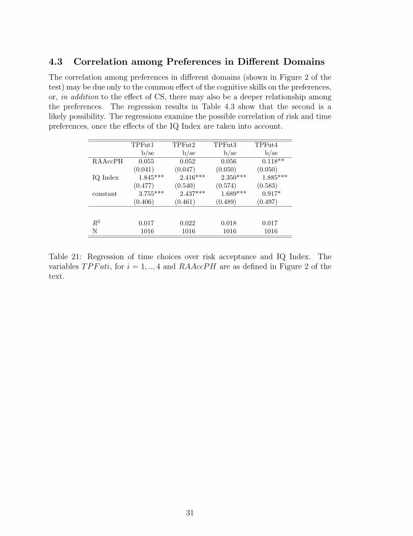
4.3 Correlation among Preferences in Different Domains

The correlation among preferences in different domains (shown in Figure 2 of thetest) may be due only to the common effect of the cognitive skills on the preferences,or, in addition to the effect of CS, there may also be a deeper relationship amongthe preferences. The regression results in Table 4.3 show that the second is alikely possibility. The regressions examine the possible correlation of risk and timepreferences, once the effects of the IQ Index are taken into account.

TPFut1 TPFut2 TPFut3 TPFut4b/se b/se b/se b/se

RAAccPH 0.055 0.052 0.056 0.118**(0.041) (0.047) (0.050) (0.050)

IQ Index 1.845*** 2.416*** 2.350*** 1.885***(0.477) (0.540) (0.574) (0.583)

constant 3.755*** 2.437*** 1.689*** 0.917*(0.406) (0.461) (0.489) (0.497)

R2 0.017 0.022 0.018 0.017N 1016 1016 1016 1016

Table 21: Regression of time choices over risk acceptance and IQ Index. Thevariables TPFuti, for i = 1, .., 4 and RAAccPH are as defined in Figure 2 of thetext.

31

5 Strategic Behavior and Cognitive Skills

{$0, $1, …, $5} {$0, $1, …, $5}

$0 $5

First mover

Second mover

Figure 3: Description of the Game: There are two players, the first and secondmovers, who move in sequence. They are both endowed with $5 by the experi-menter. The first mover has to decide unconditionally whether to transfer $0 or $5to the second mover. The second mover has to decide, before he knows the decisionof the first mover, how much he would transfer back, with a separate decision foreach of the two possible first mover actions. All amounts sent by either playerare doubled by the experimenter. Subjects gave their decisions for both roles first,after which each subject was assigned one of the two roles at random, and wasthen randomly matched with another subject who was assigned to the oppositerole. Subjects were paid according to the relevant choice each made, in the rolesassigned. Subjects also had to report their beliefs about the likely choices of theother players in the room, and were paid for correctness of their guess.

32

5.1 Beliefs and Behavior in the Game

Perc. Sending Perc. Sendingb/se b/se

IQ Index 27.886*** 21.658***(6.811) (7.910)

Numeracy 7.966(5.155)

constant 27.917*** 27.293***(5.555) (5.566)

R2 0.016 0.019N 1013 1013

Table 22: Beliefs of the first mover: Regression of the stated percentage of firstmovers sending $5.

33

Amount Amountb/se b/se

IQ Index –2.011*** –1.323**(0.450) (0.522)

Numeracy –0.879***(0.340)

constant 3.329*** 3.398****(0.367) (0.367)

R2 0.019 0.026N 1013 1013

Table 23: Beliefs of the second mover: Subject’s estimate of the amount sent backafter a transfer of $0.

The independent variable is the answer to the following question: If Person 1does send $0, what is the average amount that participants in this room will sendback? and the amount allowed was in units of 50 cents, for a total between $0 and$5.

34

Amount Amountb/se b/se

IQ Index 1.275*** 1.894***(0.474) (0.550)

Numeracy –0.792**(0.359)

constant 2.710*** 2.772***(0.387) (0.387)

R2 0.007 0.012N 1013 1013

Table 24: Beliefs of the second mover: Subject’s estimate of the amount sent backafter a transfer of $5.

The independent variable is the answer to the following question: If Person 1does send $5, what is the average amount that participants in this room will sendback? and the amount allowed was in units of 50 cents, for a total between $0 and$5.

35

Distance Distance Distanceb/se b/se b/se

IQ Index –14.039*** –10.732** –8.759*(4.232) (4.916) (5.264)

Numeracy –4.231 –4.008(3.204) (3.582)

Hit15 –0.245(0.575)

constant 40.414*** 40.746*** 39.449***(3.451) (3.459) (3.640)

R2 0.011 0.012 0.011N 1013 1013 884

Table 25: Beliefs of the first mover: Distance between the predicted and truefrequency of subjects sending $5 as first movers.

The variable Distance is the absolute value of the difference between the per-centage of subjects sending $5 as first movers and the true percentage, which is67.07 %.

36

Distance Distance Distanceb/se b/se b/se

IQ Index 0.122 0.641** 0.460**(0.277) (0.320) (0.230)

Numeracy –0.664*** –0.135(0.209) (0.156)

Hit15 –0.028(0.025)

constant 1.496*** 1.548*** 1.201****(0.226) (0.225) (0.159)

R2 0.000 0.010 0.005N 1013 1013 884

Table 26: Beliefs of the second mover: Distance between estimate and true meanin the $0 transfer.

The variable Distance is the absolute value of the difference between the Amountestimated by the subject in the event of a $0 transfer and then true mean, whichis $1.698.

37

Distance Distance Distanceb/se b/se b/se

IQ Index –0.502* 0.181 –0.367(0.299) (0.345) (0.236)

Numeracy –0.874*** –0.417***(0.225) (0.161)

Hit15 0.056**(0.026)

constant 2.046*** 2.115*** 1.840****(0.243) (0.242) (0.163)

R2 0.003 0.018 0.016N 1013 1013 884

Table 27: Beliefs of the second mover: Distance between estimate and true meanin the $5 transfer.

The variable Distance is the absolute value of the difference between the Amountestimated by the subject in the event of a $0 transfer and then true mean, whichis $3.629.

38

5.2 Behavior as First Mover

Send $5 Send $5b/se b/se

diff -0.021 -0.022***(0.017) (0.019)

IQ 0.222** 0.336***(0.115) (0.120)

diffIQ 0.036* 0.039***(0.0218 (0.022)

Age 0.006***(0.0014)

RAAcc 0.008**(0.0027)

Male 0.0102(0.049)

Credit Risk 0.001(0.000)

Other Income –0.000(0.000)

N 884 881

Table 28: Logit regression on the decision to send the $5 as first mover: Marginaleffects of IQ.

The variable diff is the difference between the expected value of sending $5 andsending $0, computed according to the estimated quantity returned by the secondmover that the subject has indicated in the elicitation of his beliefs. The variableIQ is the IQ index. The variable diffIQ is the product of diff and IQ.

39

Send $5 Send $5b/se b/se

diff 0.013*** 0.0014***(0.00389) (0.0039)

CSI 0.061*** 0.073***(0.023) (0.023)

diffCSI 0.013*** 0.012***(0.004) (0.0049)

Age 0.0073***(0.001)

RAAcc 0.0065**(0.002)

Male 0.013(0.059)

Credit Risk 0.0001(0.00008)

Other Income –0.000(0.000005)

N 884 881

Table 29: Logit regression on the decision to send the $5 as first mover: Marginaleffects of the index of Cognitive Skill

The variable diff is the difference between the expected value of sending $5and sending $0, computed according to the estimated quantity returned by thesecond mover that the subject has indicated in the elicitation of his beliefs. Thevariable CSI is the factor identified in the factor analysis of Cognitive Abilities.The variable diffCSI is the product of diff and CSI.

40

5.3 Behavior as Second Mover

Amount Amount Amount Amountb/se b/se b/se b/se

IQ Index –2.383*** –2.108*** –2.142*** –1.800***(0.453) (0.526) (0.563) (0.577)

Numeracy –0.351 0.192 0.038(0.343) (0.383) (0.393)

Hit15Index –0.582** –0.387(0.246) (0.252)

Age 0.021***(0.007)

RAAcc 0.041***(0.012)

Male –0.291(0.212)

Credit Risk –0.000(0.000)

Other Income 0.000(0.000)

constant 3.634*** 3.662*** 3.622*** 2.316***(0.369) (0.370) (0.390) (0.587)

R2 0.027 0.028 0.037 0.063N 1013 1013 884 881

Table 30: Behavior as Second Mover, After a $0 transfer.

The variable Amount is the monetary amount that the subject decides to sendback to the first mover if he transferred $0.

41

Amount Amount Amount Amountb/se b/se b/se b/se

IQ Index 1.321*** 0.829* 0.758 1.068**(0.423) (0.490) (0.526) (0.542)

Numeracy 0.630** 0.853** 0.725**(0.320) (0.358) (0.369)

Hit15Index –0.092 –0.080(0.230) (0.237)

Age 0.010(0.006)

RAAcc 0.027**(0.011)

Male 0.255(0.199)

Credit Risk 0.000(0.000)

Other Income 0.000*(0.000)

constant 2.569*** 2.520*** 2.486*** 1.006*(0.345) (0.345) (0.364) (0.551)

R2 0.010 0.013 0.016 0.034N 1013 1013 884 881

Table 31: Behavior as Second Mover, After a $5 transfer.

The variable Amount is the monetary amount that the subject decides to sendback to the first mover if he transferred $5.

42

6 Analysis of Exits from the Company

Of the 1069 subjects that participated in the study, a total of 653 had left thecompany by 4/07/2007. The table below presents a breakdown of the total exits inthree different ways, depending on whether the exit was voluntary or not, whetherit was before or after completion of training, and on whether the worker gave noticeof the exit. The final group, MIAQuit, are the “Missing in Action” drivers wholeft the company without notice.

Name of the Variable Description NumberAllExits all exits at any time for any reason 653Discharge all involuntary exits, at any time 162VolQuit all voluntary exits, at any time 491JobExit all on-the-job exits, for any reason 539TrngExit all in-training exits, for any reason 114MIAQuit all those who left without notice, at any time 142

Table 32: Reasons for exits from the job or training out of the total 1069 partici-pants. The numbers are as of 4/07/2007.

6.1 Empirical Estimates of the Survival rate

The hazard rate h(t) is as usual the ratio of the instantaneous failure rate f(t) andthe survival rate S(t):

h(t) =f(t)

S(t)

The empirical estimate of the survival rate S(t) used in the Figures in the test isthe Kaplan-Mayer estimator ([9]).

The estimated hazard rate for a subject with a vector of independent variablesx is assumed to be, following the Cox proportional hazard model,

h(t|x) = h0(t) exp(β · x)

The baseline hazard h0(t) is common to all subjects. The vector of parametersβ is estimated and indicates the effect of the individual values of the variables x.The estimated effects of each independent variable shift the baseline hazard up ordown, so a hazard rate larger than 1 indicates an increase of the hazard rate withrespect to the baseline, a rate equal to 1 means no effect, and a rate strictly lessthan 1 indicates a reduction of the hazard rate with respect to the baseline.

As noted in the test, the Kaplan Meyer survival rates show that survival isincreasing in the cognitive skill scores. The single exception is the group in thetop quintile of the Numeracy scale: individuals in this group have a survival ratesmaller than the next lower group. It is natural to imagine that a very high score

43

in numeracy makes it convenient for the driver to look for a different, perhaps morequalified, occupation, hance it may induce quitting. To keep into account the non-monotonic effect of numeracy, in the regressions below we introduce each quintilein Numeracy as a separate regressor. The non monotonic effect is confirmed: thesurvival rate of all numeracy quintiles have a higher hazard rate (lower survival)then the fourth.

6.2 Early and Late Exits

Variable Haz. Ratio St. Err. z p-valueHit15Index 0.572 0.095 -3.35 0.001IQ Index 0.547 0.198 -1.67 0.095NumQuint1 1.418 0.256 1.94 0.053NumQuint2 1.431 0.230 2.23 0.026NumQuint3 1.349 0.202 2 0.046NumQuint5 1.490 0.288 2.06 0.039Age 1.003 0.005 0.6 0.549Married 0.944 0.087 -0.63 0.527Male 1.009 0.141 0.06 0.951RAAcc 0.992 0.009 -0.84 0.398AAAcc 1.006 0.009 0.65 0.513TPFut 0.996 0.005 -0.69 0.489CreditRisk 1.000 0.000 -0.29 0.775ExperienceR 0.964 0.027 -1.34 0.179

Table 33: Hazard ratio for All Exits (AllExits): Cognitive Skills, Demographic andSocioeconomic variables. RAAcc is the total number of times the subject choosesthe lottery in the Risky choice, and AAAcc the same for the Ambiguous choices.TPFut is the total number of times the subject chooses the further payment.CreditRisk is the Credit score of the driver. ExperienceR is the length of previousexperience in on-road driving.

44

Variable Haz. Ratio St. Err. z p-valueHit15Index 0.350 0.126 -2.92 0.004IQIndex 0.536 0.381 -0.88 0.38NumQuint1 2.438 1.161 1.87 0.061NumQuint2 2.325 1.042 1.88 0.06NumQuint3 1.826 0.797 1.38 0.168NumQuint5 2.272 1.149 1.62 0.105Age 1.040 0.010 4.08 0.0001Married 0.823 0.161 -1 0.319Male 0.919 0.247 -0.31 0.753RAAcc 0.984 0.019 -0.84 0.403AAAcc 0.998 0.015 -0.1 0.918TPFut 0.990 0.010 -0.95 0.34CreditRisk 1.000 0.000 0.68 0.498ExperienceR 0.813 0.049 -3.44 0.001

Table 34: Hazard ratio for Exits during Training (TrngExit): Cognitive Skills,Demographic and Socioeconomic variables.

45

Variable Haz. Ratio St. Err. z p-valueHit15Index 0.640 0.120 -2.39 0.017IQIndex 0.548 0.217 -1.52 0.129NumQuint1 1.320 0.259 1.41 0.158NumQuint2 1.342 0.233 1.7 0.09NumQuint3 1.308 0.212 1.66 0.097NumQuint5 1.419 0.301 1.65 0.099Age 0.993 0.006 -1.18 0.237Married 0.980 0.099 -0.2 0.844Male 1.029 0.161 0.19 0.853RAAcc 0.994 0.010 -0.57 0.569AAAcc 1.007 0.010 0.73 0.465TPFut 0.998 0.006 -0.34 0.736CreditRisk 1.000 0.000 -0.47 0.64ExperienceR 1.003 0.031 0.1 0.919

Table 35: Hazard ratio for Exits on the Job (JobExit): Cognitive Skills, Demo-graphic and Socioeconomic variables.

46

References

[1] Baltagi, B. H., (2001), Econometric Analysis of Panel Data, New York, Wiley

[2] Burks, S., Carpenter, J. and Gtte, L. (2006), ”Performance Pay and the Ero-sion of Worker Cooperation: Field Experimental Evidence”, Discussion Paper#2013, Bonn, Institute for the Study of Labor (IZA)

[3] Burks S, Carpenter J, Gotte L, Monaco K, Porter K, et al. (2008) in TheAnalysis of Firms and Employees: Quantitative and Qualitative Approaches,eds. Bender S, Lane J, Shaw K, Andersson F, & von Wachter T (NBER andUniversity of Chicago)

[4] Cleveland, W.S., (1979) ”Robust Locally Weighted Regression and SmoothingScatterplots”, Journal of the American Statistical Association, December, Vol,74, No. 368, 829-836

[5] Cox, D. R., (1972), “Regression models and life tables”, Journal of the RoyalStatistical Society, B34:187-220

[6] Cox, D. R. and Oakes D., (1984), Analysis of survival data, London: Chapmanand Hall

[7] Gneezy, U., Rustichini, A. and Vostroknutov, A., (2007), “Backward Inductionas a cognitive Process”, mimeo

[8] Kahneman, D. and Tversy, A., (1979), “Prospect Theory: An Analysis of De-cision under Risk”, Econometrica, 47, 2, 263-292

[9] Kaplan E.L. and Meier P., (1958), “Nonparametric estimation from incompleteobservations”, Journal of the American Statistical Association, 53: 457-481

[10] Laibson, D., (1997). Golden eggs and hyperbolic discounting. Quarterly Jour-nal of Economics, 112, 443-477.

[11] Maccheroni, F., Marinacci, M., and Rustichini, A., (2006), “Ambiguity Aver-sion, Robustness, and the Variational Representation of Preferences”, Econo-metrica, November, 1-62

[12] Patrick, C., Curtin, J., and Tellegan, A., (2002), “Development and Vali-dation of a Brief Form of the Multidimensional Personality Questionnaire”,Psychological Assessment, Vol. 14, No. 2, 150-163

[13] Pollack, and Phelps, E, (1968). On Second-Best National Savings and Game-Equilibrium Growth. The Review of Economic Studies, 35, 2, 185-199.

[14] Raven, J.C., (2000), Ravens Standard Progressive Matrices (SPM) and RavensStandard Progressive Matrices Plus (SPM Plus), Pearson.

47