Embed Size (px)
Citation preview

Cognitive Routing for Wireless
Ad Hoc Networks
Bo Han
PhD Thesis
University of York
Department of Electronics
August 2011

Bo Han, Ph.D. Thesis Department of Electronics, University of York
2
Abstract
This thesis examines the design of cognitive routing to improve wireless ad hoc network
performance in terms of throughput and delay, as well as reducing the impact of
relaying on the network, without deteriorating end-to-end capacity. Routing metrics are
designed to replace the conventional shortest path routing metric (hop count) used in
many existing routing protocols (e.g. AODV, DSR and DSDV). The routing metrics
take into account a node/link’s surrounding environment conditions (such as disturbed
node number, bottleneck capacity, and channel utilization).
A new family of Disturbance/Inconvenience based Routing (DIR) metrics are proposed
initially, which takes both inward and outward interference into account in their weight
metric designs, in order to reduce the impact of interference in the crowded areas. Then,
a Bottleneck-Aware Routing (BAR) metric is developed to reduce bottleneck node
problems for wireless ad hoc networks. BAR not only takes an individual node’s
interference and capacity into account but is also aware of the location of bottleneck
nodes such that routes can be intelligently established to avoid congested areas, and
especially avoid bottlenecks. Under low traffic load conditions, both metrics show a
significant reduction in the congestion levels compared with the shortest path routing
metric despite increasing the relaying burden on nodes in the network.
Taking these findings into account, a cross-layer design is developed, where a Cognitive
Greedy-Backhaul (CGB) routing metric is combined with a Reinforcement Learning
based Channel Assignment Scheme (RLCAS). By applying a reinforcement learning
algorithm to the channel assignment scheme, channels can be assigned through a more
distributed and efficient approach. Moreover, the hidden node problem is mitigated and
better channel spatial reuse is achieved due to the learning within the channel
assignment scheme. By obtaining cross-layer information from the channel assignment
scheme, CGB incorporates channel utilization into its metric in order to build backhaul
links, while still utilising relatively short paths to help reduce the relaying burden. Thus,
two significant advantages can be achieved using this cross-layer design: limiting the
relaying impact and maintaining network capacity for wireless ad hoc networks. Results

Bo Han, Ph.D. Thesis Department of Electronics, University of York
3
show that this cross-layer design outperforms the other schemes in terms of energy
consumption, throughput and delay under varying traffic loads. Furthermore, the
learning progress of RLCAS is studied in a multi-hop scenario and the reason why the
learning engine of RLCAS performs well when it is associated with the CGB routing
metric is also provided.
Bo Han, Ph.D. Thesis Department of Electronics, University of York
4
Contents
Abstract .............................................................................................................................2
Contents.............................................................................................................................4
List of Tables.....................................................................................................................9
List of Figures .................................................................................................................10
Acknowledgements .........................................................................................................13
Declaration ......................................................................................................................14
1 Introduction .............................................................................................................15
1.1 Background of Wireless Ad Hoc Networks....................................................15
1.2 Advantages and Limitations of Wireless Ad Hoc Networks ..........................17
1.3 Overview of Wireless Ad Hoc Routing ..........................................................18
1.4 Purpose of the Thesis ......................................................................................20
1.5 Cognition Concept...........................................................................................20
1.5.1 Cognitive Radio.......................................................................................20
1.5.2 Cognitive Network ..................................................................................21
1.5.3 Cognitive Routing ...................................................................................22
1.6 Thesis Structure...............................................................................................24
2 Wireless Ad Hoc Routing Metrics – A Literature Review .....................................27
2.1 Introduction .....................................................................................................28
2.2 Link Quality Based Routing Metrics ..............................................................28
2.2.1 ETX .........................................................................................................28
2.2.2 ETT..........................................................................................................29
2.2.3 mETX and ENT ......................................................................................30
2.2.4 WCETT ...................................................................................................31
2.2.5 MIC .........................................................................................................33
2.2.6 iAWARE.................................................................................................35
2.2.7 Other Link Quality Based Routing..........................................................36
2.3 Non-link Quality Based Routing Metrics........................................................37
2.3.1 Hop Count ...............................................................................................37
2.3.2 Minimum Impact Routing.......................................................................39
2.3.3 Capacity-based Routing ..........................................................................40
2.3.4 PARMA...................................................................................................41

Bo Han, Ph.D. Thesis Department of Electronics, University of York
5
2.4 Routing Metric Design ....................................................................................42
2.5 Routing Protocols............................................................................................43
2.5.1 Proactive Routing Protocol – DSDV ......................................................43
2.5.2 Reactive Routing Protocols – DSR and AODV......................................44
2.5.3 Applicable Routing Protocols .................................................................46
2.6 Dijkstra’s Algorithm for Shortest Path ...........................................................47
2.7 Conclusion.......................................................................................................48
3 Modelling Techniques and Verification Methodology ...........................................49
3.1 Introduction .....................................................................................................49
3.2 Simulation Tools .............................................................................................51
3.3 Monte Carlo Simulation..................................................................................55
3.4 Validation of Results.......................................................................................58
3.4.1 Validation Using Analytical Results ......................................................58
3.4.2 Validation Using OPNET........................................................................60
3.5 Performance Parameters..................................................................................62
3.5.1 Number of Disturbed Nodes and Congestion Levels..............................63
3.5.2 End-to-end Bottleneck Capacity .............................................................63
3.5.3 Throughput and Delay.............................................................................64
3.5.4 Energy Consumption...............................................................................64
3.5.5 Time Sharing Probability ........................................................................65
3.5.6 Channel Weight.......................................................................................65
3.6 Conclusion.......................................................................................................66
4 Disturbance/Inconvenience Based Routing ...........................................................67
4.1 Introduction .....................................................................................................67
4.2 Disturbance and Inconvenience Interference ..................................................68
4.3 Disturbance/Inconvenience Based Routing Metrics .......................................70
4.3.1 DIR Link Weight Equation .....................................................................71
4.3.2 DIRk Scheme...........................................................................................73
4.3.3 DIRth Scheme..........................................................................................74
4.3.4 Analysis of Isotonicity and Monotonicity...............................................77
4.3.5 Network Environment .............................................................................80
4.4 Performance ....................................................................................................81
4.4.1 Congestion Level and Virtual Capacity ..................................................82

Bo Han, Ph.D. Thesis Department of Electronics, University of York
6
4.4.2 Snapshot Results .....................................................................................83
4.4.3 Monte Carlo Results................................................................................86
4.5 Conclusion.......................................................................................................90
5 Routing Metric Design to Improve End-to-end Bottleneck Capacity.....................92
5.1 Introduction .....................................................................................................92
5.2 Capacity Model ...............................................................................................93
5.2.1 Node Capacity .........................................................................................94
5.2.2 Node Virtual Capacity.............................................................................94
5.3 Capacity Based Routing ..................................................................................95
5.4 Bottleneck-aware Routing...............................................................................97
5.4.1 Routing Metric Design ............................................................................98
5.5 Network and Traffic Model.............................................................................99
5.6 Performance ..................................................................................................100
5.7 Conclusion.....................................................................................................105
6 Exploiting Cross-layer Design for Wireless Ad Hoc Networks ...........................106
6.1 Introduction ...................................................................................................106
6.2 Cognitive Greedy-backhaul Routing.............................................................108
6.3 Simple Channel Assignment Scheme ...........................................................111
6.3.1 Random Scheme....................................................................................112
6.3.2 Quasi-fair Scheme.................................................................................113
6.4 Network Model .............................................................................................113
6.4.1 Capacity and Throughput ......................................................................113
6.4.2 Parameters .............................................................................................116
6.5 Results ...........................................................................................................117
6.6 Conclusions ...................................................................................................120
7 Cross-layer Design Impact for CGB .....................................................................122
7.1 Introduction ...................................................................................................123
7.2 Network Model .............................................................................................124
7.2.1 Network Environment ...........................................................................124
7.2.2 Path Loss Model....................................................................................124
7.2.3 Interference Model ................................................................................126
7.2.4 Traffic Model ........................................................................................128
7.2.5 Energy Model........................................................................................128

Bo Han, Ph.D. Thesis Department of Electronics, University of York
7
7.3 Channel Assignment Schemes ......................................................................130
7.3.1 Sensing Based Channel Assignment Scheme .......................................130
7.3.2 Reinforcement Learning Based Channel Assignment Scheme.............131
7.3.3 Time Sharing and MAC Models ...........................................................136
7.4 Cognitive Cross-layer Design .......................................................................140
7.4.1 CGB with RLCAS.................................................................................140
7.4.2 SH with RLCAS and SCAS..................................................................141
7.4.3 ILR with RLCAS ..................................................................................141
7.5 Capacity Analysis..........................................................................................142
7.6 Energy Performance......................................................................................145
7.7 Delay and Throughput Performance .............................................................147
7.8 Learning Performance ...................................................................................151
7.9 Conclusion.....................................................................................................154
8 Exploiting a RL Channel Assignment Scheme.....................................................155
8.1 Introduction ...................................................................................................155
8.2 Network Scenario..........................................................................................157
8.3 RL Channel Assignment Scheme without Sensing.......................................158
8.4 Performance ..................................................................................................159
8.4.1 Network Performance ...........................................................................159
8.4.2 Learning Performance Based on Traffic Loads ....................................163
8.4.3 Learning Performance Based on Distance (hop)...................................165
8.4.4 Learning Performance Based on Link Usage........................................168
8.5 Conclusion.....................................................................................................169
9 Further Work .........................................................................................................171
9.1 The Effect of Node Mobility on Wireless Ad Hoc Routing .........................172
9.2 Cognitive Routing Protocols .........................................................................172
9.3 Network QoS Optimization...........................................................................173
9.4 Enhanced Multi-hop Reinforcement Learning Based Channel Assignment 174
9.5 Multipath Routing .........................................................................................175
10 Summary and Conclusions................................................................................176
10.1 Summary and Conclusions of the Work .......................................................176
10.2 Original Contributions...................................................................................178
10.2.1 Cognitive Routing Metric Designs........................................................179

Bo Han, Ph.D. Thesis Department of Electronics, University of York
8
10.2.2 Cross-layer Design ................................................................................180
10.2.3 Analytical Tools and Modelling............................................................181
Appendix A - Publications ............................................................................................182
Glossary.........................................................................................................................183
Bibliography..................................................................................................................185

Bo Han, Ph.D. Thesis Department of Electronics, University of York
9
List of Tables
Table 2-1 Shows the path WCETT value........................................................................32
Table 3-1 Links with the cost value for G, N-by-N sparse matrix– one of the inputs for
the “graphshortestpath” function....................................................................................53
Table 3-2 Simulation configurations...............................................................................61
Table 4-1 Key parameters of the network.......................................................................81
Table 5-1 Parameter values used in the example scenario..............................................99
Table 6-1 Parameter values used in the example scenario............................................116
Table 7-1 Parameter values used in the network...........................................................125
Table 7-2 Path loss models parameters for B5a scenario..............................................125
Table 7-3 Parameters for the path loss model ...............................................................126
Table 7-4 Modulation and coding parameters used to determine capacity and SNR ...127
Table 7-5 Weighting factor values for f1 and f2. ............................................................135
Table 7-6 Table of the time sharing scheme; N/A indicates not available; N represents
links cannot transmit at the same time; Y means links can transmit at the same time. 138
Table 8-1 Node distance table.......................................................................................166
Table 8-2 Link distance table ........................................................................................166
Bo Han, Ph.D. Thesis Department of Electronics, University of York
10
List of Figures
Figure 1-1 Cognition cycle of cognitive radio ................................................................21
Figure 1-2 Capacity routing: dotted route shows better result in terms of capacity .......23
Figure 1-3 Interference routing .......................................................................................23
Figure 2-1 Example topology where Dijkstra’s algorithm cannot find a optimum
shortest path based on the isotonic routing metric WCETT ...........................................32
Figure 2-2 An example of isotonicity .............................................................................39
Figure 3-1 Example of using “graphshortestpath” to find the shortest path in a directed
graph................................................................................................................................53
Figure 3-2 Flowchart of simulation procedure................................................................54
Figure 3-3 Example of scenario 1: homogeneous type with multiple source/sink nodes
randomly distributed in the network produced by MATLAB.........................................56
Figure 3-4 Example of scenario 2: heterogeneous type with multiple source/sink nodes
located in a grid network produced by MATLAB ..........................................................57
Figure 3-5 Example of scenario 3: homogeneous type with a common sink located
randomly in the network produced by MATLAB...........................................................57
Figure 3-6 Analytical result against simulation result ....................................................60
Figure 3-7 Square network topology produced by MATLAB........................................61
Figure 3-8 Mean value of the total number of disturbed nodes for all hops along a route
vs. link length by using MATLAB and OPNET for 32 nodes in square network ..........62
Figure 4-1: Two different types of interference associated with the node of interest
shown in black. (a) Inconvenience; (b) Disturbance.......................................................69
Figure 4-2 Example of Disturbed Nodes (DNs), Transmission Range (TR) and
Interference Range (IR)...................................................................................................70
Figure 4-3 Disturbance and inconvenience; (a) shows the disturbance level for the
selected path; (b) shows the inconvenience level for the selected path ..........................73
Figure 4-4 Network connectivity against transmission range.........................................81
Figure 4-5 Example of congestion level .........................................................................82
Figure 4-6 Contour plot of node congestion level by using SH......................................84
Figure 4-7 Contour plot of node congestion level by using DIR ....................................84
Figure 4-8 Contour plot of node congestion level by using DIR2...................................85

Bo Han, Ph.D. Thesis Department of Electronics, University of York
11
Figure 4-9 Simulation results for FTRS: (a) Mean number of hops; (b) Mean number of
DN; (c) Mean number of DN/hop vs TR ........................................................................88
Figure 4-10 Average congestion level against traffic load measured in number of active
source destination pairs ...................................................................................................90
Figure 5-1 Example of traffic through the network ........................................................95
Figure 5-2 Capacity usage at N0, including usage by interference links.........................95
Figure 5-3 Routing from A to D. The dotted route is preferred due to the link capacity is
higher on this route..........................................................................................................96
Figure 5-4 Snapshot of node congestion level by using shortest path routing metrics.102
Figure 5-5 Snapshot of node congestion level by using BAR ......................................102
Figure 5-6 CDF of long-term end-to-end bottleneck capacity with different routing
metrics ...........................................................................................................................103
Figure 5-7 Summation of end-to-end bottleneck capacity against traffic loads ...........104
Figure 6-1 Channel usage example ...............................................................................109
Figure 6-2 Shows how CGB performs (a) initial function as SH by same weight value of
1, (b) weight value reduces due to the usage, (c) backhaul links established due to the
important geographical locations; solid arrows indicate CGB path; dotted arrows show
the possible route selection by shortest path .................................................................111
Figure 6-3 Example of traffic flows through the network ............................................115
Figure 6-4 CDF of the average maximum number of channels per flow .....................118
Figure 6-5 Mean end-to-end bottleneck throughput versus traffic load........................119
Figure 6-6 Mean end-to-end bottleneck throughput versus maximum number of
channels per link............................................................................................................120
Figure 7-1 Hidden node problem; the circles indicate the transmission range of the
nodes..............................................................................................................................133
Figure 7-2 Flowchart of how RL based channel assignment function..........................136
Figure 7-3 Flowchart of time sharing scheme...............................................................137
Figure 7-4 Example of links sharing different time ......................................................138
Figure 7-5 Example of how time slots are assigned to each link..................................139
Figure 7-6 The flowchart of the MAC scheme .............................................................139
Figure 7-7 Average network energy consumption with different schemes against
network traffic load in the (a) best case scenario, (b) worst case scenario ...................147
Figure 7-8 Average delays with different schemes against network traffic load..........148

Bo Han, Ph.D. Thesis Department of Electronics, University of York
12
Figure 7-9 Average dropping probability with different schemes against network traffic
load ................................................................................................................................149
Figure 7-10 Average end-to-end throughput with different schemes against network
traffic load .....................................................................................................................151
Figure 7-11 CDF of link usage at a traffic load of 31.5 traffic flows ...........................152
Figure 7-12 CDF of channel weight value at a traffic load of 31.5 traffic flows; graph
(a) shows the extreme weight values at large reward section; graph (b) shows the
extreme weight values at large punishment section ......................................................153
Figure 8-1 Network layout ............................................................................................157
Figure 8-2 Exposed node problem ................................................................................158
Figure 8-3 Flowchart of RL without sensing based channel assignment scheme.........159
Figure 8-4 CDF of long-term end-to-end delay by using CGB with different channel
assignment schemes ......................................................................................................160
Figure 8-5 CDF of long-term end-to-end throughput by using CGB with different
channel assignment schemes.........................................................................................161
Figure 8-6 Average time sharing probability by using CGB with different channel
assignment schemes against network traffic load .........................................................162
Figure 8-7 Normalized channel weight against channel weight ranking from the highest
to the lowest at a traffic load of 13 traffic flows (low traffic load) with different channel
assignment schemes ......................................................................................................165
Figure 8-8 Normalized channel weight against channel weight ranking from the highest
to the lowest at a traffic load of 37 traffic flows (high traffic load) with different channel
assignment schemes ......................................................................................................165
Figure 8-9 Summation of highest channel weight comparison with different link
location with respect to the destination node at varying events under traffic load of 37
traffic flows ...................................................................................................................167
Figure 8-10 CDF of link usage at varying event time under traffic load of 37 flows...170
Figure 8-11 CDF of channel weight value at varying event time under traffic load of 37
flows ..............................................................................................................................170
Figure 9-1 Example of hidden node problem................................................................175

Bo Han, Ph.D. Thesis Department of Electronics, University of York
13
Acknowledgements
I would like to dedicate this thesis to my parents, as it is their continued endless love
and encouragement that has enabled me to progress my study in UK up to 9 years until
the completion of this PhD thesis.
I would especially like to thank my first supervisor, Dr. David Grace for his invaluable
advices, constant technical support and insight throughout my PhD research.
I am also grateful to my second supervisor Dr. Paul Mitchell who offered me very
useful comments and suggestions on this research work.
Further thanks go to my colleagues in the Communication Research Group for
providing a pleasant environment to work and useful discussions. In addition, my life in
the University of York could not be this fantastic and cheerful without the CSSA
(Chinese Student Society Association) and Wentworth College football team.
Finally, I would like to express my deepest thankfulness to my wife Haiqi Li, who has
been sharing happiness and facing difficulties with me.

Bo Han, Ph.D. Thesis Department of Electronics, University of York
14
Declaration
Some of the research in this thesis has been published in or submitted to conference
proceedings and journals. These papers are shown below.
• Bo Han, David Grace, Paul Mitchell, A Cognitive Cross-layer Design for
Wireless Ad Hoc Networks, Submitted to Ad Hoc Networks Journal, 2011.
• Bo Han, David Grace, Paul Mitchell, Exploring Reinforcement Learning
Channel Assignment with Cognitive Routing for Wireless Ad Hoc Networks,
in preparation for IET Communications, 2012.
• Bo Han, David Grace, and Paul Mitchell, Cognitive Greedy-Backhaul Routing
Metric Exploiting Cross-layer Design for Wireless Ad Hoc and Mesh
Networks, presented at Cognitive Radio Oriented Wireless Networks &
Communications (CROWNCOM), 2010.
• Bo Han and David Grace, Using Cognitive Interference Routing to Avoid
Congested Areas in Wireless Ad Hoc Networks, presented at Proceedings of
18th International Conference on ICCCN 2009.
• Bo Han, David Grace, and Paul Mitchell, Using Bottleneck Aware Routing to
Improve End-to-End Bottleneck Capacity for Wireless Ad Hoc Networks,
presented at Karlsruhe Workshop on Software Radios (WSR), Karlsruhe,
Germany, March, 2010.
All contributions presented in this thesis as original are, to the best knowledge of the
author. Acknowledgements and references to other researchers have been given as
appropriate.

Chapter 1. Introduction
Bo Han, Ph.D. Thesis Department of Electronics, University of York
15
Chapter 1
1 Introduction
Contents _____________________________________________________________________
1 Introduction .............................................................................................................15
1.1 Background of Wireless Ad Hoc Networks....................................................15
1.2 Advantages and Limitations of Wireless Ad Hoc Networks ..........................17
1.3 Overview of Wireless Ad Hoc Routing ..........................................................18
1.4 Purpose of the Thesis ......................................................................................20
1.5 Cognition Concept...........................................................................................20
1.5.1 Cognitive Radio.......................................................................................20
1.5.2 Cognitive Network ..................................................................................21
1.5.3 Cognitive Routing ...................................................................................22
1.6 Thesis Structure...............................................................................................24
_____________________________________________________________________
1.1 Background of Wireless Ad Hoc Networks
A rapid, self-configurable and decentralized wireless system is required for
communication service in rescue/emergency operations, military conflicts, environment
monitoring and natural disasters. Such network scenarios cannot depend on a
centralized network with organized connectivity, but they can be achieved by the
creation of wireless ad hoc networks, which are a decentralized type of wireless network
which can be created without any established infrastructure or centralized
administration. In wireless ad hoc networks, nodes are capable of functioning as routers
that are not only able to receive, but can also transmit and forward packets [1].

Chapter 1. Introduction
Bo Han, Ph.D. Thesis Department of Electronics, University of York
16
There are different types of wireless ad hoc networks that are classified according to
their applications. For instance, a mobile ad hoc network (MANET) is a self-
configuring network of mobile devices that is created via wireless links without using
centralized administration or existing network infrastructure. The network topology
changes unpredictably since the mobile nodes may move randomly in a MANET. One
typical example of applying MANETs is for communication amongst vehicles and
between vehicles and roadside units which aims to reduce car accidents via inter-vehicle
communications [2]. Another type of wireless ad hoc network is a wireless sensor
network (WSN) which in devices are sensor nodes that have less mobility compared
with MANETs and they are normally deployed in distributed locations for monitoring
environment conditions by conveying information on a hop-by-hop basis. For example,
sensor nodes can be placed in a forest to detect fires, and they can also be used to reduce
electricity/energy cost in a smart building as sensors can make the utilities more
efficient by monitoring the surroundings [3]. In addition, a wireless mesh network
(WMN) is another type of wireless ad hoc network where a hierarchical architecture is
required as mesh clients need to forward traffic to and from the gateways via access
points (mesh routers) in order to connect to the Internet. Unlike a MANET, where end
hosts and routing nodes are quite distinct and dynamic, mesh routers are usually
stationary. Therefore, due to the hierarchical architecture and stable topology, a WMN
can provide higher bandwidth and reliability than MANETs and WSNs [4]. These
different types of networks have some similarities: they are all distributed wireless
networks which use an ad hoc method as nodes are used to forward data for other nodes.
Due to the multi-hop feature of these networks, the purpose of this thesis is to
investigate how the impact of relaying can be reduced in wireless ad hoc networks by
examining routing metrics and network design while still maintaining network
performance such as capacity, throughput and delay.

Chapter 1. Introduction
Bo Han, Ph.D. Thesis Department of Electronics, University of York
17
1.2 Advantages and Limitations of Wireless Ad Hoc
Networks
Compared with cellular networks, wireless ad hoc networks are an autonomous
collection of mobile nodes which are deployed in a distributed method since there is no
need to build centralized infrastructures. Therefore, a wireless ad hoc network is a self-
configuring/healing network that can be deployed rapidly as mobile devices can join or
leave the network without jeopardizing the connectivity of the overall system. The
network size and communication services can be extended simply by deploying more ad
hoc nodes due to their multi-hop feature. Moreover, this type of network is more
reliable and resilient as each node connects to several other nodes; thus, the overall
communication system is not affected by a single node’s failure since its neighbours are
able to find an alternative route using a reliable routing protocol [3, 5, 6].
Along with these great advantages, wireless ad hoc networks also suffer some
limitations [7-11]. For instance, the network lifetime is a problem for battery-limited
portable devices, especially WSNs, as sensors are normally placed in extreme
environments such as volcanoes, oceans and forests where battery recharge or
replacement is not easy to perform. In addition, the frequent and unpredictable
movement of mobile users may result in a lack of topology information; consequently,
this can result in route oscillation and packet loss problems. The lack of centralized
monitoring also means that it may be difficult to identify incorrect operations, e.g.
broken links and selfish behaviour. Wireless ad hoc networks are more complex due to
the heterogeneous node types as each node may be equipped with different numbers or
types of radio interface that have varying transmission range or capacities. Moreover,
complex network protocols and algorithms are required for this kind of heterogeneity.
In [12], Gupta and Kumar also found that wireless ad hoc networks are considered to be
not scalable as efficiency falls rapidly with the increasing size of the network due to the
requirement of extra relaying for maintaining communication services that are far away.
This is because the limited resources are shared not only with originating traffic but also
with the relaying traffic that is required to forward the traffic on the behalf of other
nodes.

Chapter 1. Introduction
Bo Han, Ph.D. Thesis Department of Electronics, University of York
18
1.3 Overview of Wireless Ad Hoc Routing
Routing is a key feature of packet-switched networks (such as in the internet) as it
enables messages (packets) to be passed though the network from one point to another
and eventually to reach the destination [13]. The process of selecting paths to send the
traffic through the network is not only important to wired networks but also it is a core
problem in wireless networks. For wireless ad hoc networks, routing is much more
complex than in traditional wireless systems, due to the lack of centralized control and
knowledge of a predetermined topology. In order to convey messages from source node
to destination node, two choices have to be made: the routing protocol and routing
metric. The routing metric is used to select a path according to a specific design
constraint out of all available choices. The routing protocol specifies how nodes
disseminate information so that network topology can be discovered and maintained to
select routes between two nodes [14]. In other words, the routing metric is used to
calculate which route is the best to take among those available route opportunities that
are discovered by the routing protocol depending on its metric. An example of a metric
is the weight value which is learned and assigned by the routing protocol to links/nodes.
A higher weight value of a link indicates higher cost of using the link.
In wireless ad hoc networks, initially nodes are not familiar with the topology of their
networks and have to discover the topology. Ad hoc networking protocols are mainly
divided into three classes: proactive (table-driven), reactive (on-demand) and hybrid
(both proactive and reactive) protocols. In a proactive protocol, each node has an
advanced knowledge of available routing information from other nodes as routing table
updates are periodically transmitted throughout the network [15, 16]. Therefore, a
proactive protocol is more effective on route establishment as routing information is
available at each source node. Examples of proactive protocols are DSDV [17], WRP
[18], FSR [19], OLSR [20] etc. In contrast, as in the name of protocol (on-demand), the
route discovery process only takes place whenever a node has a data packet to send such
as AODV [21], DSR [22], TORA [23], ABR [24], ARA [25]. In general, proactive
protocols update route information independently of the network traffic whereas the
Chapter 1. Introduction
Bo Han, Ph.D. Thesis Department of Electronics, University of York
19
route discovery process of a reactive protocol is triggered depending on network traffic.
The hybrid protocol combines both proactive and reactive protocols, for example: ZRP
[26]. Initially, ZRP functions as a proactive protocol to find routes based on periodic
updates, and then it floods the requests of route finding on the demand of activating
nodes as a reactive protocol.
Both proactive and reactive protocols have their advantages as well as disadvantages.
Proactive protocols have better knowledge of routing information to all destinations,
therefore result in a rapid process of route establishment. Moreover, they react faster to
topology changes due to their consistent up-to-date route discovery process.
Nonetheless, they consume network capacities for nodes that are not in use and have a
significant control overhead in generating routing information for maintaining the
network topology. On the other hand, reactive protocols save bandwidth and energy due
to the comparatively fewer activities in the route discovery process although they create
a longer delay when discovering routes. Under a high traffic load, networks can be
congested by the flooding of route request packets due to the high demands of route
finding. For a hybrid protocol, although it could have both the advantages of proactive
and reactive protocols, performance is mainly limited by the number of active nodes and
it generates more complexity for the route discovery process since it is using both
proactive and reactive techniques.
Since the routing protocols can discover the network topology and available relaying
choices, another challenge of routing is to determine which paths are suitable to select
among all the options. There are many different routing metrics available in wireless ad
hoc networks, such as number of hops, link utilization, latency, packet loss, energy,
throughput, interference, load-balancing and so on. By manipulating link cost/weight,
routes can be selected differently with varying routing metrics to achieve different
goals. Lots of routing metrics have been proposed for wireless ad hoc networks, such as
hop count [21, 22], ETX [27], ETT [28], WCETT [28], ENT [29] etc. More details of
these listed metrics will be reviewed in the next chapter.

Chapter 1. Introduction
Bo Han, Ph.D. Thesis Department of Electronics, University of York
20
1.4 Purpose of the Thesis
As aforementioned, wireless ad hoc networks have been suggested as a method of peer-
to-peer communications, removing the need for fixed infrastructures. Such methods
work well when the number of relay hops is small, but their efficiency falls rapidly in
homogeneous ad hoc networks when the number of relay hops increases, due to the fact
that additional capacities are required to carry information on a hop-by-hop basis. The
capacity is considered to be surprisingly low in wireless ad hoc networks [30].
Many works focused on the design of efficient routing protocols to deal with moving
nodes and topology maintenance due to the dynamic features of wireless ad hoc
networks. Less attention has been paid on the choice of routes in wireless ad hoc
networks. Therefore, this thesis is to investigate how the impact of relaying can be
reduced in wireless ad hoc networks by examining routing metrics and channel
assignment schemes while still maintaining network capacity with increasing traffic
loads.
1.5 Cognition Concept
To understand the term ‘cognitive routing’, which is one of the main aspects of this
thesis, it is necessary to introduce two related subjects – cognitive radio and cognitive
networks.
1.5.1 Cognitive Radio
Cognitive radio has been proposed as a paradigm for wireless communications that can
utilize the radio frequency spectrum in a more efficient way as it has the ability to
change its transmitter parameters (operating spectrum, modulation, transmit power)
based on interactions with the surrounding spectral environment [31]. Based on the
cognitive concept, the cognitive radio technique provides the opportunity for unlicensed

Chapter 1. Introduction
Bo Han, Ph.D. Thesis Department of Electronics, University of York
21
users to share the radio spectrum with licensed users without degrading their services
[32].
The fundamental objective of cognitive radio is to identify sub-bands of the radio
spectrum that are currently unemployed and assign them to unlicensed secondary users
[33]. In order to extend this concept to include interaction with the environment, a
cognition cycle is introduced. Figure 1-1 shows the cognition cycle. By the process of
observing the environment, orienting itself, creating plans, then deciding and acting, the
cognitive radio can finally achieve its goals [31, 34].
Figure 1-1 Cognition cycle of cognitive radio
1.5.2 Cognitive Network
Modern communication networks face challenges on the efficient management of
increasing complexity as networks are composed of many heterogeneous nodes, links
and users. In addition, those networks are often operating under dynamic environments
where network resources (e.g. node energy and channel assignment), application data
(e.g. the location of data) and user behaviours (e.g. user mobility) change over time [35].
All those factors can degrade network performance and they are beyond the limit of
manual administration. In order to maintain a good quality service based on as little
human intervention as possible, a cognitive network paradigm is proposed [36, 37]. A
cognitive network is a network with a cognitive process that can perceive current
network conditions, and then plan, decide and act on those conditions. The network can

Chapter 1. Introduction
Bo Han, Ph.D. Thesis Department of Electronics, University of York
22
learn from these adaptations and use them to make future decisions, all the while taking
into account the end-to-end goals [38].
Cognitive networks should be self-aware and have a self-managing ability that means
they should have knowledge about themselves as well as their own environment, and
can plan and execute appropriate actions in a decentralized way. The self-aware feature
of a radio is claimed to be ‘cognitive’ in [31]. Extending this cognition concept beyond
the radio domain (layer 1 and layer 2) to cover all the layers of the OSI model is the
difference between cognitive radio and cognitive networks.
The definition is similar to the definition of cognitive radio as both of them need to
learn, adapt and react to their environment to achieve a certain goal, but the
performance of the cognitive network is measured by end-to-end rather than point-to-
point.
1.5.3 Cognitive Routing
Before introducing the term “cognitive routing”, some general concepts about routing
are presented to help the reader to understand the ideas. Routing is a process of selecting
paths. In order to serve goal of the network level (e.g. finding the shortest path), there
must be a certain mechanism to comprehensively link the nodes in the network and
allow them to establish routes in a collective way.
Conventional routing algorithms normally find the route with the shortest path to
improve efficiency [28]. However, in a wireless ad hoc network, shortest path routing is
not necessarily the best solution. First of all, more efficient routing metrics can be
achieved by taking other factors into account, such as capacity, delay, link length,
spectrum availability, power throughput and/or interference rather than just considering
hop number. Figure 1-2 demonstrates a case where the longer route in terms of hop
number (dashed path) is preferred due to its higher link capacity than the short route
(solid path) as the thick dotted lines indicate higher capacity due to a high level of
interference caused at node C in this graph. The longer link is better as the links with

Chapter 1. Introduction
Bo Han, Ph.D. Thesis Department of Electronics, University of York
23
higher capacity can carry more relaying traffic and can reduce the burden of
bottleneck(s) in the network. Also, regarding the complicated radio environment due to
interference, a longer route could be a better choice than a short route, if the node on the
shorter route suffers/causes more severe interference from/to other node(s) (see Figure
1-3). If a node suffers from serious interference, it could significantly decrease the
effective capacity for the routing traffic request; if it causes too much interference to
neighbouring nodes, others may suffer a great deal in terms of effective capacity [39].
Figure 1-2 Capacity routing: dotted route shows better result in terms of capacity
Figure 1-3 Interference routing
As aforementioned, a cognitive radio ‘is a radio that can change its transmitter
parameters based on interaction with the environment where it operates’ [11], and
additionally relevant here is the radio’s ability to look for, and intelligently assign,
spectrum ‘holes’ on a dynamic basis from within primarily assigned spectral
allocations. A cognitive network ‘is a network with a cognitive process that can
A
B
C
E
A
B
C
E D

Chapter 1. Introduction
Bo Han, Ph.D. Thesis Department of Electronics, University of York
24
perceive current network conditions, and then plan, decide, and act on those conditions’
[10]. Given the combination of cognitive radio and cognitive networking aspects in this
thesis, we refer to this collective process as cognitive routing. For the routing
mechanism to be ‘cognitive’, it must have three types of process: observing, reasoning
(calculating) and acting (adapting) [14, 15]. In this thesis, we focus on the calculating
process mainly, assuming the necessary information for each node is available through
observing and different adjustments can be carried out in terms of acting.
Due to the aforementioned cognitive concept, here we define cognitive routing as a
routing selection process that not only can perceive and utilize varying link conditions
based on its metric design (e.g. link distance between the transmitter and the receiver,
interference, energy cost, channel capacity and loss rate), but also can improve network
performance in the future by the decision of current route selection. As aforementioned,
the purpose of this thesis is to design a routing metric that can reduce relay hops while
still maintain network capacity by associating cognitive radio techniques. A
reinforcement learning based channel assignment scheme is applied to assign channels
in a decentralized manner. Therefore, in this thesis, the cognitive routing metric is
specified to be able to perceive channel assignment or interference information, utilize it
and improve the future learning efficiency of the channel assignment scheme by the
current routing selection process. Cognitive greedy-backhaul (CGB) routing metric is an
example of cognitive routing in Chapter 7 as it is not only aware of the channel
assignment situation in the network, but more importantly it makes the reinforcement
learning based channel assignment in a more efficient and faster way (results will be
shown in Chapter 7).
1.6 Thesis Structure
The thesis is divided into 8 further chapters and the structure is outlined as follows.
Chapter 2 introduces the background information of this thesis which is a literature
review on wireless ad hoc routing metric design. The review investigates, summarises
and comments on those wireless ad hoc routing metric designs. In addition, routing

Chapter 1. Introduction
Bo Han, Ph.D. Thesis Department of Electronics, University of York
25
protocols include DSDV (a proactive routing protocol), DSR and AODV (reactive
routing protocols) are also described to help the reader to understand the routing process
as a whole. Dijkstra’s Algorithm is also presented as a technique to find the lowest cost
path for all routing metric designs in this thesis.
Chapter 3 presents the simulation techniques and software tools that are used to conduct
the research work. In addition, the verification methodology is provided along with the
main parameters to evaluate the performance of the proposed routing metrics.
Chapter 4 reviews a routing metric design known as minimum impact routing (MIR)
which aims to reduce the interference when selecting routes. It is then followed by a
proposed family of interference based routing metric designs inspired by MIR, known
as disturbance/inconvenience based routing (DIR) which can take both ‘inward’ and
‘outward’ interference into account. By manipulating a priority factor, routes can be
selected in a more altruistic (outward) or selfish (inward) manner. Two classes of DIR
have been given to study the interference on wireless ad hoc networks, DIRk and
DIRthreshold. A discussion of the interference of the two classes of DIR on network
performance is also provided.
Chapter 5 illustrates the capacity model used in this thesis. It also presents a bottleneck
node problem and its impact on wireless ad hoc networks. Then two routing metrics,
capacity based routing (CBR) and bottleneck-aware routing (BAR) are studied to
investigate how the bottleneck problem can be mitigated. Performance and conclusions
are also given.
Chapter 6 proposes a cross-layer design by combining the routing metric with the
channel assignment scheme to reduce the relaying burden while still maintaining
bottleneck capacity. The cross-layer design starts with two simple channel assignment
schemes. Simulation and results are also given to illustrate the importance of the
channel assignment scheme for this cross-layer design.
In chapter 7, a practical network model is developed by including a more realistic
network environment, including more sophisticated propagation, interference, traffic

Chapter 1. Introduction
Bo Han, Ph.D. Thesis Department of Electronics, University of York
26
and energy models. A sensing based channel assignment scheme and a reinforcement
learning based channel assignment scheme are also introduced to perform the cross-
layer design with varying routing metrics. In addition, time sharing and MAC schemes
are also embedded in to the network. Network performance is tested when applying the
reinforcement learning based channel assignment scheme with varying routing metric
designs. One of the routing metric designs, CGB, is analysed to illustrate the reason
why it can perform an efficient learning process on channel selections with a
reinforcement learning based channel assignment scheme.
Rather than analyse the network performance by examining reinforcement leaning
based channel assignment schemes with different routing metric designs as in Chapter
7, chapter 8 looks at a different perspective by using varying channel assignment
schemes with the same routing metric design. A pure sensing based channel assignment
scheme, pure reinforcement learning based channel assignment scheme (without the
assistance of any sensing technique) and a reinforcement learning based channel
assignment scheme plus sensing are all associated with the CGB routing metric.
Network performance is tested for the schemes in terms of throughput and delay.
Chapter 9 describes modifications, improvements and potential work that may further
improve the capacity of wireless ad hoc networks. This is followed by the overall
summary and conclusions in chapter 10.

Chapter 2. Wireless Ad Hoc Routing Metrics – A Literature Review
Bo Han, Ph.D. Thesis Department of Electronics, University of York
27
Chapter 2
2 Wireless Ad Hoc Routing Metrics – A
Literature Review
Contents _____________________________________________________________________
2 Wireless Ad Hoc Routing Metrics – A Literature Review .....................................27
2.1 Introduction .....................................................................................................28
2.2 Link Quality Based Routing Metrics ..............................................................28
2.2.1 ETX .........................................................................................................28
2.2.2 ETT..........................................................................................................29
2.2.3 mETX and ENT ......................................................................................30
2.2.4 WCETT ...................................................................................................31
2.2.5 MIC .........................................................................................................33
2.2.6 iAWARE.................................................................................................35
2.2.7 Other Link Quality Based Routing..........................................................36
2.3 Non-link Quality Based Routing Metrics........................................................37
2.3.1 Hop Count ...............................................................................................37
2.3.2 Minimum Impact Routing.......................................................................39
2.3.3 Capacity-based Routing ..........................................................................40
2.3.4 PARMA...................................................................................................41
2.4 Routing Metric Design ....................................................................................42
2.5 Routing Protocols............................................................................................43
2.5.1 Proactive Routing Protocol – DSDV ......................................................43
2.5.2 Reactive Routing Protocols – DSR and AODV......................................44
2.5.3 Applicable Routing Protocols .................................................................46
2.6 Dijkstra’s Algorithm for Shortest Path ...........................................................47
2.7 Conclusion.......................................................................................................48
_____________________________________________________________________

Chapter 2. Wireless Ad Hoc Routing Metrics – A Literature Review
Bo Han, Ph.D. Thesis Department of Electronics, University of York
28
2.1 Introduction
This chapter provides the relevant background information to the research work.
Initially we categorize wireless ad hoc routing metric designs into two types: non-link
quality based routing and link quality based routing. The literature review of each type
of routing metric is shown. Then several well-known wireless ad hoc routing protocols
are discussed to aid understanding of the routing process. A discussion of which type of
routing protocol is more applicable to associate with our proposed routing metrics is
also presented.
2.2 Link Quality Based Routing Metrics
ETX is designed to make the routing metric aware of link quality rather than just the
simple hop count in order to improve network performance. The awareness of link
quality is considered to be favourable for routing metric design in multi-hop wireless
networks especially for ad hoc and mesh networks. Consequently, a large number of
routing metrics are modified or extended based on ETX to improve routing metric
design by considering other factors (interference, channel diversity, load balancing etc.).
Here, we will give a literature review on the most significant link quality routing
metrics such as ETX, ETT, WCETT, MIC, iAWARE etc.
2.2.1 ETX
Expected Transmission Count (ETX) [27] was the first mesh metric design to take link
quality into account in multi-hop wireless networks. The ETX of a link is defined as the
expected number of data transmissions that are needed for successfully delivering a
packet over that link. It is proposed to find high-throughput paths by taking link
delivery ratios of both forward (df) and reverse (dr) direction into account. The metric is
defined as below.

Chapter 2. Wireless Ad Hoc Routing Metrics – A Literature Review
Bo Han, Ph.D. Thesis Department of Electronics, University of York
29
rf ddETX
⋅=
1
(2.1)
The path is selected based on the minimum sum of ETX along the route to the
destination. Since each node periodically broadcasts probe packets to its neighbours, the
delivery ratio (df and dr) can be measured by the number of received probes (at the
receiver or transmitter respectively) at the last T time interval in a sliding window
fashion.
ETX is also an isotonic routing metric. It takes into account delivery ratios which
directly affects throughput as well as loss ratio asymmetry in both directions of each
link since loss ratio equals one minus the delivery ratio. In addition, the metric reflects
the effect of both loss ratio and path length. However, ETX does not cope well with a
network which has a high transmission data rate and larger packet size due to the fact
that broadcasts are normally performed at the network basic rate and probe packets are
relatively small, so that the metric cannot reflect the loss rate of actual traffic. In
addition, the metric does not consider load-balancing and does not take any channel
conditions into account [14, 40-43].
2.2.2 ETT
Expected Transmission Time (ETT) is proposed as a “bandwidth-adjusted ETX” by
Draves et al. [28]. The metric is a function of the loss rate and the bandwidth of a link
and it improves the ETX metric by further considering the differences in link
transmission rates. The function of ETT is defined below.
B
SETXETT ⋅=
(2.2)
Where S indicates the size of a probing packet and B is the bandwidth of the link. The
ETT metric modifies the ETX metric by multiplying by the time spent in transmitting
the packet.

Chapter 2. Wireless Ad Hoc Routing Metrics – A Literature Review
Bo Han, Ph.D. Thesis Department of Electronics, University of York
30
Therefore, ETT has the advantages of ETX as well as the improvement of taking link
capacities into consideration to increase the throughput on the path. Nonetheless, the
disadvantages of ETT remain, in that the metric does not take account link load, path
length and channel diversity.
2.2.3 mETX and ENT
Koksal and Balakrishnan [44] proposed another two link quality-aware routing metrics
mETX and ENT which are modified versions of ETX. The ETX routing metric is
considered to work well in relatively static wireless channel conditions as it uses the
mean loss ratios in making route decisions and packet loss probability shows a
significant long-term dependence [40]. However it has a shortcoming to cope with
short term channel or fast link-quality variations, e.g., it cannot adapt well to burst loss
conditions even with a low average packet loss ratio of the channel due to its high
variability.
mETX is defined as follows:
21exp
2µ σΣ Σ = +
mETX (2.3)
where µ∑ indicates the estimated average packet loss ratio of a link; σ2∑ is the variance
of this value. These two parameters of a channel are estimated by considering the
locations of errored bits in each probe packet. A loss rate sample is calculated for every
ten probe packets that are sent out by each node like ETX [27].
Unlike ETX and mETX, ENT also considers the number of retransmissions into the
routing metric design which limits route computation to links that show an acceptable
number of retransmissions according to upper-layer requirements. The ENT routing
metric is defined as follows:
Chapter 2. Wireless Ad Hoc Routing Metrics – A Literature Review
Bo Han, Ph.D. Thesis Department of Electronics, University of York
31
( )2exp 2µ δσΣ Σ= +ENT (2.4)
where δ indicates the certain threshold number of retransmissions which will determine
the link layer protocol’s decision to give up a sending attempt.
The time-varying characteristics of a wireless channel are captured by both of the
mETX and the ENT and they could be directly translated into network and application
layer quality constraints [44].
2.2.4 WCETT
Draves et al. also proposed a Weighted Cumulative ETT (WCETT) [28] which is an
extended version of ETT considering end-to-end delay and channel diversity. Therefore,
the metric is composed of two parts as shown below.
jkj
n
i
i XETTWCETT≤≤
=
+−= ∑1
1
max)1( ββ (2.5)
Where n is the number of hops along the path; k is the total number of channels
available in the system; Xj is the sum of transmission times of hops on channel j; finally,
β is a tuneable parameter which is between 0 and 1 .This separates the priority impact of
different parts of the weight function. The first part of the function ∑=
n
i
iETT1
enables
WCETT to account for the estimated end-to-end delay experienced by a packet
travelling along the path over n hops. Since neither ETX nor ETT is designed for
multiple-channel networks, simply adding up the ETT of each individual link cannot
reflect an optimum path in a multi-channel network due to the intra-flow interference
which can reduce the overall performance of the entire path. Therefore, in order to
account for the channel diversity in multi-channel networks, the second part of the
function jkjX
≤≤1max is included to reflect the sum of transmission times on the bottleneck

Chapter 2. Wireless Ad Hoc Routing Metrics – A Literature Review
Bo Han, Ph.D. Thesis Department of Electronics, University of York
32
channel due to its heavy usage. Consequently, it shows the feature that a path with more
channels assigned on their links is preferable due to the lower weights.
Although WCETT takes intra-flow interference into its metric design, the metric does
not explicitly consider inter-flow interference. Hence, it may lead activated traffic flows
to congested areas. Moreover, the metric is not isotonic which may not guarantee a
shortest path. An example topology is shown in Figure 2-1 which illustrates that
Dijkstra’s algorithm cannot find the shortest path based on the isotonic routing metric of
WCETT. Considering the path from S→A→B, the estimated end-to-end delay is 0.4 as
ETT from S→A is 0.2 and ETT from A→B is 0.2, and j
kjX
≤≤1maxβ is 0.2 as both channel 2
and channel 3 has same delay of 0.2. Therefore, the WCETT of path S→A→B is 0.3
when β is 0.5. Considering the path from S→B directly, the WCETT is 0.45. Therefore,
Dijkstra’s algorithm will go through the path S→A→B rather than S→B directly due to
the smaller WCETT value. However, considering a path is required from S to D and the
link from B to D also uses channel 3, then jkjX
≤≤1max (the sum of transmission times on
the bottleneck channel) is changed significantly from 0.2 to 0.7. Therefore, the correct
shortest path should be from S→B→D due to the smallest WCETT value as shown in
Table 2-1. However, WCETT incorrectly selects the other one (S→A→B→D) as
Dijkstra’s algorithm has determined the shortest path from S to B is through S→A→B.
Figure 2-1 Example topology where Dijkstra’s algorithm cannot find a optimum shortest path
based on the isotonic routing metric WCETT
Path ∑=
n
i
iETT1
jkjX
≤≤1max WCETT (β = 0.5)
S→B→D 0.95 0.5 0.725
S→A→B→D 0.9 0.7 0.8
Table 2-1 Shows the path WCETT value
Chapter 2. Wireless Ad Hoc Routing Metrics – A Literature Review
Bo Han, Ph.D. Thesis Department of Electronics, University of York
33
Therefore, WCETT cannot be applied to all routing protocols as it is unable to find a
shortest path and solve looping problem.
2.2.5 MIC
Yang et al. [45] proposed a metric of interference and channel-switching (MIC) in order
to solve the issues of WCETT, which are non-isotonic routing and non-awareness of
inter-flow interference. The weight path function of MIC is defined as:
∑∑∈∈
+=pinode
i
pllink
l CSCIRUpMIC α)( (2.6)
where p stands for a path in the network, IRU and CSC stand for interference-aware
resource usage and channel switching cost respectively, which are defined later. α is a
trade-off value to make sure that the IRU is around the same value range as the value of
CSC, and is defined as follows:
)min(
1
ETTN ⋅=α
(2.7)
where N indicates the number of nodes in the network and min(ETT) is the smallest ETT
in the network, which can be estimated based on the lowest transmission rate of the
wireless cards.
IRU (Interference-aware Resource Usage) captures the differences in the transmission
rates, loss ratios of wireless links as well as the inter-flow interference, and CSC
(Channel Switching Cost) captures the intra-flow interference. They are defined as
follows:
lll NETTIRU ⋅= (2.8)
Chapter 2. Wireless Ad Hoc Routing Metrics – A Literature Review
Bo Han, Ph.D. Thesis Department of Electronics, University of York
34
21
2
10,
)())((
)())((ww
iCHiprevCHifw
iCHiprevCHifwCSC i <≤
=
≠=
(2.9)
where Nl is the set of neighbour nodes that the transmission on link interferes with,
CH(i) indicates the channel assigned for node i’s transmission and prev(i) presents the
previous hop of node i along the path. The relationship of w2>w1 captures the fact that a
higher cost is imposed if node i and prev(i) use same channel due to the intra-flow
interference. In [45], w1 is set to 0 and the value of w2 is from 0.3 to 5. Therefore, due to
the component of IRU, MIC favours a path that consumes less channel times at its
neighbouring nodes. The CSC part of MIC represents the metric’s ability to deal with
the intra-flow interference as it provides a higher weight value for the consecutive links
if they use the same channel. Therefore, the path with more diversified channel
assignments is preferred by the MIC.
It is worth mentioning that MIC is not isotonic if it is applied directly to real networks.
Therefore, the authors [45] introduced virtual nodes which are images of real nodes into
the network and thereafter guarantee the shortest loop-free path by decomposing MIC
into isotonic link weight assignments on virtual links between these virtual nodes.
Although the MIC routing metric aims to account for inter-flow interference by scaling
up the ETT of a link by the number of neighbours interfering with the transmission of
that link, the interference level caused by each interferer node is not the same in practice
as it depends on the SINR value at the receiver of the link (which includes the
interferer’s signal strength, locations with respect to the object link’s receiver and path
loss characteristics etc.). Moreover, the CSC part of MIC only considers the intra-flow
interference when the links are consecutive. This is imprecise as interference can be 3-
hops away along a same path due to the fact that interference range is always much
larger than transmission range in real life [46].

Chapter 2. Wireless Ad Hoc Routing Metrics – A Literature Review
Bo Han, Ph.D. Thesis Department of Electronics, University of York
35
2.2.6 iAWARE
The interference aware routing metric (iAWARE) [47], is proposed to capture the effect
of variations of link loss ratio, differences in transmission rate as well as intra-flow and
inter-flow interference. Unlike the MIC, the iAWARE metric captures the intra-flow
and inter-flow interference using a physical interference model by calculating the signal
to noise ratio (SNR) and signal to interference and noise ratio (SINR).
The link metric, iAWARE of a link i is defined as:
i
i
iIR
ETTiAWARE =
(2.10)
where IRi(u) refers to an interference ratio of a node u in a link i = (u,v) which is bigger
than 0 and smaller or equal to 1 as defined:
)(
)()(
uSNR
uSINRuIR
i
i
i = (2.11)
Thus, considering a bidirectional communication link i = (u,v) for a DATA/ACK-like
communication, the interference ratio of a link i (IRi) is defined as:
))(),(min( vIRuIRIR iii = (2.12)
The weighted cumulative path metric iAWARE(p) of a path p is defined as follows.
jkj
n
i
i XiAWAREpiAWARE≤≤
=
+−= ∑1
1
max)1()( αα (2.13)
where α is a tunable parameter set between 0 and 1; k is the number of orthogonal
channels available; n is the number of hops along the path p; the part of Xj indicates that
the iAWARE is aware of the channel diversity and the intra-flow interference as it is
defined as:

Chapter 2. Wireless Ad Hoc Routing Metrics – A Literature Review
Bo Han, Ph.D. Thesis Department of Electronics, University of York
36
kjiAWAREXjchannelonilinksgConflictin
ij ≤≤= ∑ 1, (2.14)
Although the iAWARE uses a practical interference model to continuously reproduce
the neighbouring interference variations onto routing metrics, the routing metric is not
isotonic due to the second component like WCETT.
2.2.7 Other Link Quality Based Routing
There are other link quality based routing metrics and although they are not as popular
as the aforementioned link quality based routing metrics, they are introduced here to
provide a broad background information of wireless ad hoc routing metrics.
In [48], Zhai et al. proposes a routing metric known as interference clique transmission
time (CTT) to take account of the multi-rate capability (the capability of supporting
multiple channel rates) with the packet loss ratio (ETX) in order to maximize the end-
to-end throughput. Although this metric selects the path which has the maximum end-
to-end bottleneck capacity, it produces an excessive relaying burden and it is not
isotonic [49].
Genetzakis, et al. [49] proposes a contention-aware transmission time (CATT) metric
which takes both contentions of the shared wireless channel and rate diversity in multi-
radio multi-channels into account. The performance of using CATT is improved by
using ETX and ETT as it captures both the number of interfering links and the level of
their interference. In addition, it is an isotonic routing metric. However, the scalability
of using CATT is not examined due to the limited number of test nodes and again it
fails to take path distance into account.
The multi-channel routing (MCR) metric is proposed by Kyasanur et al. [50] to deal
with multiple channel, multi-interface networks. The metric does not only select
channel diverse paths like WCETT, but also modifies WCETT to incorporate switching

Chapter 2. Wireless Ad Hoc Routing Metrics – A Literature Review
Bo Han, Ph.D. Thesis Department of Electronics, University of York
37
cost, so that it prevents selecting paths that require frequent channel switching. The
major limitation of this metric is that it does not completely account for inter-flow
interference as all channels are considered as orthogonal [43].
Tsai et al. proposed a weighted interference multipath [51] metric which aims to achieve
better reliability and low delay by taking the path interference (which reflects the degree
of intra-flow interference between the links which use the same channel along the path)
and the neighbour interference (which represents the channel time cost to nodes close to
the path) into account.
2.3 Non-link Quality Based Routing Metrics
The routing metrics that are not extended from ETX are considered as non-link quality
based in this work. The other routing metrics design may take network parameters (such
as energy, throughput, delay, channel usage etc.) rather than link quality into their
metrics design. In this section, the conventional routing metric (Hop Count), minimum
impact routing (MIR) [52] and capacity-based routing (CBR) [53] are presented.
2.3.1 Hop Count
Traditional wireless ad hoc routing protocols, such as DSDV, AODV and DSR, use hop
count as their routing metrics. This is the simplest routing metric as the metric only
considers whether a link exists or not. The route is selected based on the smallest
number of hops along the path. Therefore, it can be easily computed and the hop count
minimised from the source to the destination once the topology is identified. Such a
simple algorithm can react quicker than other routing metrics in rapidly changing
topologies. Another advantage of hop count is the isotonicity and monotonicity, so that
using an efficient algorithm (Bellman-Ford or Dijkstra’s algorithm) can find loop-free
and optimum paths with minimum total cost. In the following, we use mathematic
functions to illustrate the meaning of isotonicity and monotonicity for routing metrics.
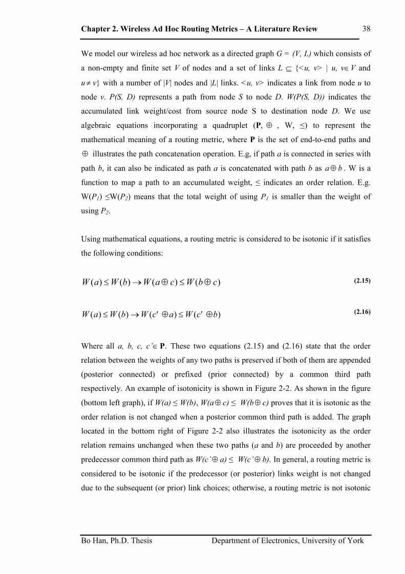
Chapter 2. Wireless Ad Hoc Routing Metrics – A Literature Review
Bo Han, Ph.D. Thesis Department of Electronics, University of York
38
We model our wireless ad hoc network as a directed graph G = (V, L) which consists of
a non-empty and finite set V of nodes and a set of links L ⊆ {<u, v> | u, v∈V and
u≠ v} with a number of |V| nodes and |L| links. <u, v> indicates a link from node u to
node v. P(S, D) represents a path from node S to node D. W(P(S, D)) indicates the
accumulated link weight/cost from source node S to destination node D. We use
algebraic equations incorporating a quadruplet (P, ⊕ , W, ≤) to represent the
mathematical meaning of a routing metric, where P is the set of end-to-end paths and
⊕ illustrates the path concatenation operation. E.g, if path a is connected in series with
path b, it can also be indicated as path a is concatenated with path b as ba⊕ . W is a
function to map a path to an accumulated weight, ≤ indicates an order relation. E.g.
W(P1) ≤W(P2) means that the total weight of using P1 is smaller than the weight of
using P2.
Using mathematical equations, a routing metric is considered to be isotonic if it satisfies
the following conditions:
)()()()( cbWcaWbWaW ⊕≤⊕→≤ (2.15)
)'()'()()( bcWacWbWaW ⊕≤⊕→≤ (2.16)
Where all a, b, c, c’∈P. These two equations (2.15) and (2.16) state that the order
relation between the weights of any two paths is preserved if both of them are appended
(posterior connected) or prefixed (prior connected) by a common third path
respectively. An example of isotonicity is shown in Figure 2-2. As shown in the figure
(bottom left graph), if W(a) ≤ W(b), W(a⊕ c) ≤ W(b⊕ c) proves that it is isotonic as the
order relation is not changed when a posterior common third path is added. The graph
located in the bottom right of Figure 2-2 also illustrates the isotonicity as the order
relation remains unchanged when these two paths (a and b) are proceeded by another
predecessor common third path as W(c’⊕ a) ≤ W(c’⊕ b). In general, a routing metric is
considered to be isotonic if the predecessor (or posterior) links weight is not changed
due to the subsequent (or prior) link choices; otherwise, a routing metric is not isotonic

Chapter 2. Wireless Ad Hoc Routing Metrics – A Literature Review
Bo Han, Ph.D. Thesis Department of Electronics, University of York
39
if the predecessor (or posterior) links weight can be affected by the subsequent (or prior)
link choices.
A routing metric is considered to be monotonic if it satisfies the following conditions:
)()( baWaW ⊕≤ (2.17)
)()( acWaW ⊕≤ (2.18)
Where all a, b, c∈P. Here, monotonicity implies the weight of a path does not decrease
when prefixed or appended by another path. In other words, non-negative values have to
be used to enable the routing metric to be monotonic [54].
( ) ( )bWaW ≤
( ) ( )cbWcaW ⊕≤⊕ ( ) ( )bcWacW ⊕≤⊕ ''
Figure 2-2 An example of isotonicity
Although the simplicity and stability of hop count routing metrics are useful
characteristics for wireless ad hoc routing metric design, the metric does not take other
factors (e.g. interference, link capacity and channel utilization) into account which may
result in a poor performance on route establishment.
2.3.2 Minimum Impact Routing
In wireless ad hoc networks, system capacity is considered interference-limited as only
a limited number of users can communicate simultaneously due to interference between
transmitting nodes and surrounding nodes sharing the same spectrum. Thus, it is

Chapter 2. Wireless Ad Hoc Routing Metrics – A Literature Review
Bo Han, Ph.D. Thesis Department of Electronics, University of York
40
important to consider the interference on the transmitters and receivers in an ad hoc
network. Interference information is useful when making higher-layer decisions such as
routing. Conventional routing metrics such as hop count fail to take interference into
account. In [52], Lu et al. proposed a Minimum Impact Routing (MIR) which selects
the route based on the lowest number of disturbed nodes (DN) along the path in order to
minimise the interference to other nodes.
Minimum Impact Routing (MIR) aims to minimise the number of disturbed nodes
(DNs) for a multi-hop transmission, thereby enhancing the overall spectral efficiency. It
selects a route that has the lowest disturbance impact between the source node and
destination node. MIR only takes the disturbance (outward) interference into account.
Here the link weight of MIR is defined as:
VjiD
wj
ij ∈∀= ,,1
(2.19)
Where Dj is the disturbance level which is the number of disturbed nodes of node j. The
Minimum Impact Routing metric picks the path with the lowest cost of accumulated
disturbed nodes from s to d in the network T.
Although MIR aims to reduce the overall interference by minimizing the number of
end-to-end disturbed nodes along the path, it fails to account for the fact that practical
interference is based on the disturbed transmitter power, path loss, etc. In addition, MIR
encourages traffic flow through less congested areas which results in creating longer
paths and increases the relaying burden in the network.
2.3.3 Capacity-based Routing
In [53], Liu et al. proposed a cognitive routing metric design called Capacity-based
Routing (CBR) which takes varying link capacity into account in order to improve the
capacity of wireless ad hoc networks by selecting nodes/links with higher capacity. It
also aims to reduce the overall interference level by shifting traffic to the edge of the

Chapter 2. Wireless Ad Hoc Routing Metrics – A Literature Review
Bo Han, Ph.D. Thesis Department of Electronics, University of York
41
network where there is less interference. However, CBR is not considered as cognitive
routing (see page 25) as it only observes and utilises node capacity without the
technique of reasoning and an acting process to improve network capacity. Although it
can improve network capacity when network traffic load is low by shifting the path to
the edge of the network, it cannot maintain network capacity when more traffic arrives
as it will generate more relaying hops to avoid congestion areas. The unstable route
selection process cannot assist the reinforcement learning based channel assignment
scheme on its channel selection (results will be shown in Chapter 7), therefore network
capacity is reduced. The link weight of CBR is defined by [53]:
VjiC
wj
ij ∈∀= ,,1
(2.20)
where Cj indicates the capacity of node j. By using Dijkstra's algorithm, which is
introduced later in this chapter, CBR prefers to select nodes with higher capacities and
routes that are established based on the maximisation of the accumulated impact
capacity has on an end-to-end basis.
In [53], link capacity is related to the total number of activated links within the
interference range of the link as well as the available bandwidth (more details about
how the capacity model is defined can be found in Chapter 5). Although CBR can
cognitively take the varying link capacity which reflects the traffic pattern and
interference into account, the lack of selecting the shortest path can even increase the
interference under medium or high traffic load networks.
2.3.4 PARMA
In [55], Zhao et al. proposed a PHY/MAC aware routing metric for wireless ad hoc
networks (PARMA) which takes into account factors including physical-layer link
speed and MAC-layer channel congestion. It aims to minimize the end-to-end delay that
includes both transmission and access times by comparison with traditional minimum
hop count routing metric. Although the routing metric uses cross-layer information to

Chapter 2. Wireless Ad Hoc Routing Metrics – A Literature Review
Bo Han, Ph.D. Thesis Department of Electronics, University of York
42
avoid those links with low data rate and high retransmission rate due to the busy
medium, it does not take path stability and path length into the metric design. These two
factors are important for routing metric design as dynamic routing (low path stability)
provides inefficient channel assignment which reduces the efficiency of MAC schemes,
and longer paths indicate a higher relaying burden which requires more bandwidth to
accommodate extra relaying traffic. Finally, end-to-end delay can be improved by using
PARMA under low traffic conditions, but networks are easily saturated due to the
insufficient network capacity under high traffic demands.
2.4 Routing Metric Design
Although the research work on routing metric designs is increasing, there is no
consensus solution for wireless ad hoc routing metrics. In addition, there is a trend for
metrics that are increasingly complicated taking into account multiple link/network
factors in order to improve routing performance. Therefore, in this thesis, we aim to
design a simple wireless ad hoc routing metric that not only can account for channel
diversity in a multichannel environment, but can also react back to the distributed
channel assignment scheme to make the future channel selection in a more efficient
way. Although aforementioned WCETT [28] and MIC [45] have awareness of channel
diversity, their route establishment have no impact on the channel assignment scheme.
Moreover, their route establishment may consume even more radio resources due to the
unawareness of path length and route stability. Chapter 7 proposes a cognitive routing
metric design (CGB) which uses channel utilization level to build routes and it also
provides an efficient channel selection process for a reinforcement learning based
channel assignment scheme (results are shown in Chapter 8). This cognitive routing is
performed firstly by monitoring and perceiving current network conditions including
interference, channel utilization, load balancing and relaying burden impact; then
planning, deciding and acting on those conditions, learning from the consequences of its
actions, and finally through learning a routing decision can be made in order to achieve
end-to-end goals.
Chapter 2. Wireless Ad Hoc Routing Metrics – A Literature Review
Bo Han, Ph.D. Thesis Department of Electronics, University of York
43
2.5 Routing Protocols
In Chapter 1, we listed several traditional wireless ad hoc routing protocols including
proactive routing protocols (DSDV and WRP), reactive routing protocols (AODV and
DSR) and hybrid routing protocols (ZRP). The advantages and disadvantages of each
type of routing protocol were also pointed out. Due to the scope of the thesis which is to
design cognitive routing metrics that can take into account environmental factors in the
link weight function instead of traditional hop count in order to minimize relaying
impact on the network while still maintaining network capacity, throughput and delay
under different traffic load conditions, only a few routing protocols are discussed in the
thesis for the purpose of understanding the integrated wireless ad hoc routing process as
a whole.
2.5.1 Proactive Routing Protocol – DSDV
Amongst proactive (table-driven) routing protocols, Destination-Sequenced Distance
Vector (DSDV) protocol is one of the most famous and the earliest routing protocols,
and was presented by C. Perkins and P.Bhagwat in 1994 [17]. It applies a modified
version of the Distributed Bellman-Ford algorithm (DBF) [56, 57] to solve the poor
looping properties (count to infinity) caused by incorrect route information (broken
links). DSDV is proposed to solve these route looping problems by introducing a
frequent dynamic update on detecting topology changes. This is achieved by each node
periodically broadcasting routing updates in order to obtain updated information on the
network topology. The routing update is tagged with a sequence number which can
distinguish stale or incorrect routes from recent ones. A route is considered to be
preferred if its sequence number is greater than the others. To maintain consistency of
route information under frequent changes of topology, each node transmits its routing
table packets periodically and incrementally once topological changes are detected.
Update information from each node consists of the target destination’s address, number
of hops required to reach the destination and its new sequence number regarding that
destination. If the same sequence number occurs among different paths, the smallest
metric will be selected to forward packets. With the periodic routing information

Chapter 2. Wireless Ad Hoc Routing Metrics – A Literature Review
Bo Han, Ph.D. Thesis Department of Electronics, University of York
44
updates and newest sequence number, each node can obtain the correct shortest path to
each other node quickly regardless of the topology changes which can result in stale or
incorrect route information.
There are two types of update packets used to reduce routing overhead: “full dumped”
which carries all the available routing information and “incremental” which carries only
information which differs from the last full dump. Although these two types of update
are introduced to reduce routing information, DSDV still generates a large amount of
routing overhead due to the requirement of periodic routing messages, especially within
a large network. Therefore, network bandwidth is wasted by exchanging these frequent
routing messages among all nodes even when the network is idle.
2.5.2 Reactive Routing Protocols – DSR and AODV
In order to reduce unnecessary bandwidth waste caused by routing overheads in
proactive routing protocols especially when the network is idle, reactive routing
protocols are often proposed which only send out route request packets when a node has
packets to send [14, 16]. This means routes are only determined on demand rather than
maintained all the time by the continuous periodic updating in proactive protocols.
Generally, reactive routing protocols can be further classified into two categories:
source routing and hop-by-hop routing [16]. In source routing, each data packet
contains the complete source to destination route whereas a node only needs to know
the source and destination as well as next hop routing information in hop-by-hop
routing. One of the best known reactive protocols which uses source routing is Dynamic
Source Routing (DSR) [22], which is composed of two mechanisms: route discovery
and route maintenance. Route discovery is used only when a node has packets to send to
a destination and does not already know a route to the destination. To initiate route
discovery, route request messages of the original source node are flooded into the
network in a controlled manner. Nodes send a route reply back to the original source
node with their route records to the destination node if they know a way to the
destination or if they are the destination itself. Nodes that receive the route request

Chapter 2. Wireless Ad Hoc Routing Metrics – A Literature Review
Bo Han, Ph.D. Thesis Department of Electronics, University of York
45
message and do not know the destination will append their own address to the route
record in the request packet and then broadcast the request to their neighbours. In this
way, route discovery costs can be limited as each node maintains a cache of routes it has
heard. Route maintenance is achieved by acknowledgements and route error messages
when a source route is no longer valid due to the change of network topology. The
sender can then find an alternative valid route from its route cache or can invoke the
route discovery process again to find a new route; route maintenance is only performed
when the source node is actually sending packets to the destination.
The main advantage of source routing is that nodes do not need to periodically send
beacon messages to their neighbours to inform them of their presence. Another
advantage is that intermediate nodes do not need to maintain up-to-date routing
information for each activated route as complete routing information is kept in each
packet header. The major disadvantage compared with hop-by-hop routing is the
routing information overhead grows as the number of intermediate nodes increases
along the route [16, 41].
Ad hoc On-Demand Distance Vector (AODV) Routing is one of the best known hop-
by-hop reactive routing protocols, and was developed by C. Perkins, E. Belding-Royer
and S. Das [21] in order to further reduce routing overhead problems. AODV combines
both essential mechanisms of DSDV and DSR. It applies the sequence number and
periodic beacons on a hop-by-hop basis from the DSDV mechanism, as well as the on-
demand route discovery process from DSR. Unlike DSR, when route request packets
accumulate route information through each intermediate node along the path, the
request packet of AODV only contains the source and destination as well as the next
hop; therefore a large amount of routing information can be reduced by using AODV
due to the hop-by-hop basis. Also due to the hop-by-hop basis, HELLO packets are
required to be sent locally and periodically to maintain connectivity among the
neighbourhoods, similar to the routing table update of DSDV. Moreover, AODV also
applies the sequence number of DSDV in order to avoid loop and count-to-infinity
problems as well as avoiding stale routing information caused by link breakages. The
main advantage of using AODV over DSR is that it is more adaptable in relatively large
and dynamic networks.

Chapter 2. Wireless Ad Hoc Routing Metrics – A Literature Review
Bo Han, Ph.D. Thesis Department of Electronics, University of York
46
To sum up, DSR is better for use in a small and stable network as the route cache of
each node contains multiple valid routes; therefore if a source node finds a valid route in
its route cache, it does not need to initiate a route discovery process which saves
network bandwidth for flooding. In contrast, AODV can cope better than DSR in a
relatively large and dynamic network as it uses better up-to-date paths due to its
sequence number.
2.5.3 Applicable Routing Protocols
In this thesis, we examine routing metrics in a static wireless ad hoc network without
node movement and we assume no link or node failure takes place. Since the traditional
routing algorithm/metric is the hop count, which results in a fixed value for each link
weight if the network topology is stable and the links are reliable, once a source node
obtains a route to a destination, this route will always be valid and with minimum cost
under those assumptions and conditions. In this way, Route Request packets will not be
flooded for routes that have been utilized before; thus, routing messages are reduced and
network bandwidth is saved. Therefore applying a reactive routing protocol seems to be
a wise option for a relatively stable network topology.
However, in this thesis, we are trying to examine different routing metrics by taking
‘cognition’ which includes network environment factors (such as interference, load
balancing, link capacity, throughput, channel assignment) into account rather than a
simple hop account; hence, cost/weight value of each link may differ every time a new
source traffic is activated as those metrics are likely to be affected by traffic flows even
with a stable network topology. In this way, a new shortest path is always requested as
the previous one may no longer be valid due to the highly dynamic changing feature on
routing metrics. The reactive routing protocol is not suitable for this type of routing
metric design as the excessive flooding due to the frequent route requests increases the
amount of routing overheads and reduces network bandwidth. Therefore, a proactive
routing protocol is used to evaluate the cognitive routing metric designs proposed in this
thesis.

Chapter 2. Wireless Ad Hoc Routing Metrics – A Literature Review
Bo Han, Ph.D. Thesis Department of Electronics, University of York
47
2.6 Dijkstra’s Algorithm for Shortest Path
In this thesis, Dijkstra’s algorithm [58] is selected to solve the shortest path problem for
a given graph with link weight/cost values, for all routing metrics. The functionality of
Dijkstra’s original algorithm can be extended for various purposes. For example, the
OSPF (open shortest path first) protocol is an implementation of Dijkstra’s algorithm
for Internet routing [58]. Dijkstra’s algorithm can effectively select the route with the
lowest accumulated cost. In order to achieve higher level goals in the system, we can
exploit the optimization function of Dijkstra’s algorithm by redefining the cost. That is
to say, the definition of cost is manipulated in order to serve a different purpose [53].
Consider a directed graph G = (V, L) which consists of a non-empty and finite set V of
nodes and a set of links L ⊆ {<u, v> | u, v∈V and u≠ v} with a number of |V| nodes
and |L| links. <u,v> and wu,v indicates a link from node u to its adjacent node v and the
cost respectively. Dijkstra’s algorithm keeps two sets of vertices. One is the set of
vertices whose shortest path from the source have already been determined (we call it
the visited set, S). The other one is the set with remaining vertices (we call it the
unvisited set, V-S). Let d denotes the shortest cost from the source vertex to the current
vertex. Given a path π in G determined by the Dijkstra’s algorithm. p(v) denotes the
Predecessor of v for any v in π (v≠s). The following execution steps show how to find a
shortest path by using Dijkstra’s algorithm from source node s to destination node x:
Initial Stage:
1. Set S to empty
2. Set p(v) to empty
3. Set the cost from source vertex to other vertices to be infinity, d(s,v) = ∞
4. Set the cost from source to itself to be 0, d(s,s) = 0
This initial stage sets up the graph so that each node has no predecessor and the
estimates of the distance of each vertex from the source are infinity, except for the
source itself.

Chapter 2. Wireless Ad Hoc Routing Metrics – A Literature Review
Bo Han, Ph.D. Thesis Department of Electronics, University of York
48
Repeat Stage:
1. Find the vertex (u) from the unvisited set (V-S) that gives the shortest distance to the
source
2. Process the vertices (v) still in V-S connected to u and check whether the current
best estimate of shortest distance to v can be improved by going through u: If d(s,v)
> d(s,u) + wu,v, then d(s,v) = d(s,u) + wu,v and let p(v) = u.
3. Take node u as visited. i.e. S = S∪ {u},
4. If u = x, the Dijkstra’s algorithm process terminates as the shortest path has been
discovered from the source s to the destination x, otherwise return to the first step of
the repeat stage.
The other well known algorithm that is often used to find the shortest paths in a network
is Bellman-Ford. Although Bellman-Ford can work with negative cost where Dijkstra’s
algorithm cannot, it is slower to find the shortest paths than Dijkstra’s algorithm since it
relaxes all edges by |V|-1 times rather than greedily selects the unvisited minimum cost
node. Conventional routing algorithms normally find the shortest path route with
minimum hop count to improve efficiency [28]. However, in a wireless ad hoc network,
the minimum hop count is not necessarily the best solution. First of all, the diverse
capacity levels due to different link length, spectrum availability and/or power level can
be used more efficiently if the cognitive routing metric design takes them into account.
2.7 Conclusion
In this chapter, the relevant background information of this research work has been
provided. Initially, three main types of wireless ad hoc routing protocol are shown with
detailed examples, and the reason for using proactive routing protocol for this research
work is also given. This is followed by a literature review on wireless ad hoc routing
metric design with a detailed discussion on the limitations and merits of those existing
routing metrics. Dijkstra’s algorithm is described as a method to find the shortest path.
Finally, cognitive radio and cognitive network have been introduced to illustrate the
concept of cognitive routing.

Chapter 3. Simulation Techniques and Verification Methodology
Bo Han, Ph.D. Thesis Department of Electronics, University of York
49
Chapter 3
3 Modelling Techniques and Verification
Methodology
Contents _____________________________________________________________________
3 Modelling Techniques and Verification Methodology ...........................................49
3.1 Introduction .....................................................................................................49
3.2 Simulation Tools .............................................................................................51
3.3 Monte Carlo Simulation..................................................................................55
3.4 Validation of Results.......................................................................................58
3.4.1 Validation Using Analytical Results ......................................................58
3.4.2 Validation Using OPNET........................................................................60
3.5 Performance Parameters..................................................................................62
3.5.1 Number of Disturbed Nodes and Congestion Levels..............................63
3.5.2 End-to-end Bottleneck Capacity .............................................................63
3.5.3 Throughput and Delay.............................................................................64
3.5.4 Energy Consumption...............................................................................64
3.5.5 Time Sharing Probability ........................................................................65
3.5.6 Channel Weight.......................................................................................65
3.6 Conclusion.......................................................................................................66
_____________________________________________________________________
3.1 Introduction
The purpose of this chapter is to present the wireless ad hoc routing evaluation methods
utilized throughout this thesis before introducing the main research work. There are

Chapter 3. Simulation Techniques and Verification Methodology
Bo Han, Ph.D. Thesis Department of Electronics, University of York
50
different approaches for engineers to conduct their research. Each approach has its
merits and flaws for varying types of research work. Computer simulation is one of
most widely used and efficient methods for communications researchers. Robert E.
Shannon defines simulation as the process of designing a model of a real system and
conducting experiments with this model for the purpose of understanding the behaviour
of the system and evaluating various strategies for the operation of the system [59].
Researchers can use the technique to imitate some real particular systems or to
implement system scenarios that are not possible in the real world. Therefore, the
advantages of selecting simulation as the main method of evaluation are due to the
characteristic of low cost and the feature of flexibility. With the growing complexity of
wireless communications architecture and scenarios, analytical models are expensive
and sometimes impossible to implement, whereas the scenario configurations of
simulation models can be easily adjusted and results can be reproduced as needed. In
addition, thanks to the development of computing technology, powerful computers and
sophisticated simulation software are available to allow a more accurate behaviour
modelling of wireless communications. Moreover, it is extremely difficult to effectively
model the behaviour of networks and systems with analytical models since modern
network architectures are quite complicated; and the main intention of this research was
to design a novel technique to associate a cognitive routing metric with a distributed
channel assignment scheme in wireless ad hoc networks, in order to reduce network
relaying hops while still maintain network capacities. Therefore, simulation has been
chosen as the main approach to conduct the works in this thesis.
This chapter firstly describes the details of the Monte Carlo simulation technique. In the
following section, the introduction of the simulation tool MATLAB is presented in
comparison with other widely used simulation tools and languages. Next, the
parameters used to evaluate the network performance are shown and a validation
method is discussed. The chapter ends with a brief conclusion.

Chapter 3. Simulation Techniques and Verification Methodology
Bo Han, Ph.D. Thesis Department of Electronics, University of York
51
3.2 Simulation Tools
Nowadays, there are many simulation programming tools available to perform
simulations in communication engineering research. Although many programming tools
are capable of conducting simulations in communications research, each one has its
unique features that can achieve certain needs of research easier than the others as well
as its limitations. E.g. C programming has the advantage on the speed of run-time due to
its straight-forward compiled rather than interpreted language so the machine
instructions can be executed more efficiently, but as the mother of modern languages
[60], it needs more programming to achieve the functions of other programming tools,
for example, it requires more external programmed loops to solve matrix problems
whereas these can be solved easily in MATLAB, as will be discussed in more detail
later. OPNET and NS2 are popular network simulators for communication research as
they have many built-in simulation models, which include many standard
communication protocols across different layers for designers to test new networking
protocols or to modify the existing protocols using packet-level analysis. The
disadvantages of these network simulators are that the simulations require more
processing power and time due to the radio pipeline stage, especially in the case of
OPNET as it is designed for cable/wire networks. Therefore with radio networks 'virtual
wires' are effectively generated to provide connectivity, with packets being duplicated
from the source to each node, even if only interference is being calculated. Each of
these packets then goes through a 12 stage receiver pipeline. Moreover, as the purpose
of this thesis is to reduce relaying hops while maintaining network capacity by
designing cognitive routing metrics with reinforcement learning based channel
assignment scheme, the efficient modelling of mutual interference is critical, and
MATLAB and C can be custom designed to model this efficiently. In addition, the
simulation analysis is mainly focused on the link/flow based transmissions rather than
the packet based transmissions. Regarding the reinforcement learning based channel
assignment scheme (details can be found in Chapter 7 and 8), links will have a preferred
channel or channels after a period time of learning process. In order to process the
channel weight of links in a more efficient way, MATLAB is selected as it has better
computational flexibility than the others.

Chapter 3. Simulation Techniques and Verification Methodology
Bo Han, Ph.D. Thesis Department of Electronics, University of York
52
MATLAB is the abbreviation for Matrix Laboratory developed by MATHWORKS Inc
[61]. In addition to those highlighted above, there are several other advantages of using
MATLAB rather than other high-level programming languages for this research work.
Since it is an interpreted language for numerical computation, it can compute numerical
calculations such as array, matrix and cell, and is reasonably efficient without the need
for complicated programming. In addition, there are many built-in or predefined
functions and varying toolboxes for users to perform different kinds of simulations in a
more efficient way. For example, one of the functions, “graphshortestpath [62]” which
is a built-in function from the Bioinformatics toolbox, is frequently used in this thesis. It
has the ability to solve the shortest path problem using graphs and it can return values
including every node on the path and the path cost. The function is shown below.
[ ] ),,(,, TSGestpathgraphshortpredpathdist = (3.1)
Where dist is the path cost value; path contains every node along the path; and pred
contains the predecessor nodes of the path. G is the N-by-N sparse matrix which
contains the cost/weight of each link/edge. S and T are the source node and destination
node respectively. Figure 3-1 Example of using “graphshortestpath” to find the shortest
path in a directed graphshows an example of using “graphshortestpath” function to find
the shortest path from node 1 to node 4, and the content of links with the cost from G is
shown in Table 3-1.

Chapter 3. Simulation Techniques and Verification Methodology
Bo Han, Ph.D. Thesis Department of Electronics, University of York
53
Figure 3-1 Example of using “graphshortestpath” to find the shortest path in a directed graph
(4,1) 0.6000
(1,2) 0.1000
(2,3) 0.3000
(6,3) 0.8000
(7,3) 1.0000
(3,4) 0.5000
(6,4) 0.9000
(2,5) 0.4000
(7,5) 2.0000
(5,6) 0.7000
(1,7) 0.2000
Table 3-1 Links with the cost value for G, N-by-N sparse matrix– one of the inputs for the
“graphshortestpath” function
As can be seen from the example, dist is 0.9 and path returns [1 2 3 4] as the shortest
path which relays through node 2 and 3. This single syntax provides a shortest path and

Chapter 3. Simulation Techniques and Verification Methodology
Bo Han, Ph.D. Thesis Department of Electronics, University of York
54
its cost value as well as the graphical result by using the built-in function from the
Bioinformatics toolbox. These built-in functions allow users to produce code efficiently.
Moreover, it offers a friendly interface for users to trace any errors and debug easily due
to its interactive programming feature. MATLAB is selected as the main simulation tool
for our research work, despite its slower execution, as we consider the simulation
development speed is more important than the simulation speed. Simulation can take a
long time, but can run without user intervention (during a day or overnight). MATLAB
has been used to capture the features of each routing metric design in wireless ad hoc
networks and the simulation procedures are illustrated in Figure 3-2.
Figure 3-2 Flowchart of simulation procedure

Chapter 3. Simulation Techniques and Verification Methodology
Bo Han, Ph.D. Thesis Department of Electronics, University of York
55
3.3 Monte Carlo Simulation
The impact of applying different types of routing metric in wireless ad hoc networks is
studied in this thesis by using the Monte Carlo simulation technique. Monte Carlo
simulation is a classic computational algorithm for communication engineers. It relies
on repeated random sampling to generate statistical results and determine the behaviour
of the system. A large number of sets are provided to perform the simulation in order to
reduce the effect of random fluctuations enabling the statistical certainty of the result to
become more precise [63].
There are three different types of wireless ad hoc network scenario used in this thesis.
We consider nodes have no mobility throughout the thesis. One implements
homogeneous nodes in random distributed locations and varying sink nodes are selected
as shown in Figure 3-3. This scenario is applied in Chapter 4 to understand the
challenges of routing metric design in wireless ad hoc networks. Another one is the
heterogeneous scenario with different types of node located in a grid network.
Aggregation nodes (with higher capacity than normal nodes) are randomly distributed in
the middle of the network and landmark nodes (with highest capacity) are implemented
on both edges of the network as shown in Figure 3-4. This scenario is used in Chapter 5
to investigate the bottleneck node problem of wireless ad hoc networks. The last
scenario uses homogenous node types with random locations through the network and a
common sink node is selected in the middle of the network as shown in Figure 3-5. This
is similar to a battlefield scenario where the headquarters receives/sends the messages
from/to the army nearby. The scenario is applied in Chapters 6, 7 and 8 to improve the
network QoS, capacity, bottleneck problems of wireless ad hoc networks by varying
routing metric designs.
The reason of using two network scenarios for random node placements with
dimensions of 40 km and 550 meters respectively is as follows. The early scenario (40 ×
40 km2) is focused on designing and investigating how link weight can be manipulated
by extending the metric design of MIR [52]. In [52], varying radio link length is
adopted in three different topologies: hexagon, square and chain. In order to further
analyse how well MIR can route traffics around dense areas in a random topology, the
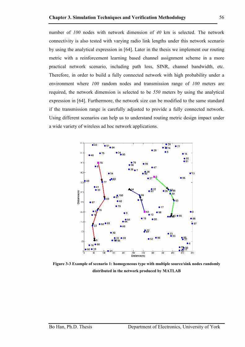
Chapter 3. Simulation Techniques and Verification Methodology
Bo Han, Ph.D. Thesis Department of Electronics, University of York
56
number of 100 nodes with network dimension of 40 km is selected. The network
connectivity is also tested with varying radio link lengths under this network scenario
by using the analytical expression in [64]. Later in the thesis we implement our routing
metric with a reinforcement learning based channel assignment scheme in a more
practical network scenario, including path loss, SINR, channel bandwidth, etc.
Therefore, in order to build a fully connected network with high probability under a
environment where 100 random nodes and transmission range of 100 meters are
required, the network dimension is selected to be 550 meters by using the analytical
expression in [64]. Furthermore, the network size can be modified to the same standard
if the transmission range is carefully adjusted to provide a fully connected network.
Using different scenarios can help us to understand routing metric design impact under
a wide variety of wireless ad hoc network applications.
Figure 3-3 Example of scenario 1: homogeneous type with multiple source/sink nodes randomly
distributed in the network produced by MATLAB

Chapter 3. Simulation Techniques and Verification Methodology
Bo Han, Ph.D. Thesis Department of Electronics, University of York
57
Figure 3-4 Example of scenario 2: heterogeneous type with multiple source/sink nodes located in a
grid network produced by MATLAB
Figure 3-5 Example of scenario 3: homogeneous type with a common sink located randomly in the
network produced by MATLAB

Chapter 3. Simulation Techniques and Verification Methodology
Bo Han, Ph.D. Thesis Department of Electronics, University of York
58
3.4 Validation of Results
Performance analysis of wireless ad hoc networks is very challenging due to the facts
that such analysis must to take into account the network topology, radio propagation,
multiple access, routing, traffic patterns, etc. In this section, we will apply two methods
to validate our simulation result. Firstly, possible analytical approaches are discussed,
such as capacity analysis in wireless ad hoc networks, to provide a performance
comparison with our simulation framework in Chapter 7 and 8. Secondly, our early
simulation framework (in Chapter 4) of using MATLAB is compared with a previously
published result [52] from an independently-written simulator (OPNET).
3.4.1 Validation Using Analytical Results
Several studies have focused on finding the maximum achievable capacity on a per-
node basis. E.g. in [12], it is shown that each node can obtain Θ( nnW log/ ) bits per
second. In [30], the authors examined the dependence of per-node capacity on 802.11
MAC interactions and traffic patterns for various simple network topologies, such as a
single cell, chain, uniform lattice and random network.
Here, we will examine wireless ad hoc network throughput on a per-flow basis by
considering current traffic flows and present an analytical model that takes into account
network size, traffic flows, radio range and maximum transmission rate. Our simulation
framework is verified by comparing with the analytical results and the similarities and
differences between the two are discussed.
Consider a network with n identical randomly located nodes (no mobility) within a
square area of A, each node is capable of transmitting at W bits per second over a
common channel and a perfect scheduling algorithm, which knows the locations of all
nodes and all traffic demands, is applied. Then transmissions can be coordinated
temporally and spatially to avoid collisions. If such perfect information is not available,
the throughput is smaller.

Chapter 3. Simulation Techniques and Verification Methodology
Bo Han, Ph.D. Thesis Department of Electronics, University of York
59
Let L denote the expected distance that a packet traverses from a source node to a
destination node and r the common range of all transmissions. Then, the expected
number of hops taken by packets is no less than r
L in a connected network [12]. If the
number of traffic flows is known as λ, therefore the expected number of activated links
is no less than λr
L . We can obtain the lower bound end-to-end throughput of a traffic
flow if no spatial reuse is considered here. In other words, all transmissions interfere
with each other, so they can only obtain one portion of the channel for its transmission
which is W divided by the number of activated links under the perfect scheduling
approach. For shortest path routing metric which generates minimum number of hops
amongst all routing metrics, the expected end-to-end throughput of a path is
approximately λLWr .
The analysis of no spatial reuse is a worst case scenario as no transmissions can occur
simultaneously. However, transmissions that are far away can occur simultaneously,
provided there is no excessive interference on both sides. This spatial concurrency and
frequency reuse can intuitively increase the end-to-end throughput of a traffic flow.
In Chapter 7 and 8, the common destination is selected at the centre of the network.
Therefore, we can estimate the expected path length (L) of using shortest path routing
metric for a random traffic pattern, which is 3
2 A (more details about this can be found
in Chapter 7). Due to the aforementioned equations, we can deduce the end-to-end
throughput by using shortest path routing metric in terms of transmission capability,
transmission range, traffic flows and network size:
A
rWC
λ23
= (3.2)
Considering the throughput analysis on a per-flow basis, the minimum number of traffic
flows is 1. Therefore, we can obtain the end-to-end throughput of one traffic flow as

Chapter 3. Simulation Techniques and Verification Methodology
Bo Han, Ph.D. Thesis Department of Electronics, University of York
60
L
Wr . For the scenario where a common destination is selected at the centre of the
network, the end-to-end throughput on a path is:
A
rWC
2
3=
(3.3)
In Figure 3-6, analytical and simulation results are presented for the end-to-end
throughput analysis. The simulation result is obtained in a single channel environment
with a network dimension of 550 meters. The transmission range of nodes is 100 meters
and the destination node is selected at the centre of the network. The maximum channel
capacity is 9 Mbps. No spatial concurrency is considered in the simulation as each link
competes for the channel capacity with all the others. The end-to-end throughput of
analytical and simulation results follows an exponential drop with increasing the level
of traffic load. It is observed that the simulation results agree closely with the
theoretical values.
Figure 3-6 Analytical result against simulation result
3.4.2 Validation Using OPNET
Chapter 4 presents our early simulation work using MATLAB to reduce traffic
congestion in the dense area by routing traffic through the edge of the network. This is
done by a routing metric design, Minimum Impact Routing (MIR) which selects routes

Chapter 3. Simulation Techniques and Verification Methodology
Bo Han, Ph.D. Thesis Department of Electronics, University of York
61
based on the lowest number of disturbed nodes (DNs) along the path. More details of
this routing metric can be found in Chapter 4 and [52]. Here, we will validate our
simulation results by using MATLAB, compared with the results obtained by using
OPNET in [52]. The network parameters used here are the same as in [52], and they are
listed in Table 3-2. The interference range is twice the transmission range. The square
network topology that is produced by MATLAB is shown in Figure 3-7.
Routing metric MIR
Network size 16 x 16 km
Node spacing 2.5 km
Network topology Square
Number of nodes 32
Radio link length 3, 6, 9, 12, 15, 18, 21 km
Route selection criteria Minimum number of DNs
Table 3-2 Simulation configurations
Figure 3-7 Square network topology produced by MATLAB
Figure 3-8 shows the performance in terms of the mean value of the total number of
disturbed nodes for all hops along a route against various radio link lengths by using
MATLAB, compared with OPNET in [52]. The results of mean DNs along a path are

Chapter 3. Simulation Techniques and Verification Methodology
Bo Han, Ph.D. Thesis Department of Electronics, University of York
62
collected through 2000 different source-to-destination pairs and those sources and
destinations are selected based on a uniform distribution. As can be seen from this
figure, MATLAB obtains similar results in terms of mean DNs as when OPNET is
used. MIR has a lower number of DNs when the transmission range increases. This is
expected as hop number is decreased when transmission range is increased, and
therefore, there are fewer alternative choices of route and the number of DNs is similar.
When the link length increases to a link length of 16 km (interference range is 32 km),
the node which is located at the centre of the network would expect the mean number of
DNs to be 30 (excluding itself and the receiver node) as all nodes are within its
interference range.
Figure 3-8 Mean value of the total number of disturbed nodes for all hops along a route vs. link
length by using MATLAB and OPNET for 32 nodes in square network
3.5 Performance Parameters
Different routing metrics will be presented in the following chapters for optimizing
different applications of wireless ad hoc networks. In wireless sensor networks (WSN),
energy/power consumption is considered to be more important than other network
parameters as sensors are deployed in places where the battery is very difficult or
expensive to recharge or replace. In wireless mesh networks (WMNs), quality of service
(QoS) is the primary goal rather than energy consumption as it has a relatively stable
topology and access points (AP) can be easily replaced or discarded without losing

Chapter 3. Simulation Techniques and Verification Methodology
Bo Han, Ph.D. Thesis Department of Electronics, University of York
63
connectivity to the gateway. In mobile ad hoc networks (MANET), maintaining routing
information to continuously carry the communication service seems to be the primary
challenge due to the mobility of the devices [5]. Although the goals are different,
depending on the types of the wireless ad hoc network, the primary target of this
research is to design cognitive routing metrics with a distributed channel assignment
scheme that can reduce relaying hops while still maintaining network capacity.
3.5.1 Number of Disturbed Nodes and Congestion Levels
The number of disturbed nodes and the congestion level are used initially to help us to
understand routing metric behaviour in wireless ad hoc networks. The disturbed node
(DN) is defined as a node within the interference range of the node of interest [52]. The
congestion level of a node is defined as the total number of activated links within the
interference range of the node [53]. More details of the parameters can be found in
Chapter 4 and 5. These two parameters can examine the altruistic feature of routing
metrics as by taking the disturbed node number into the metric design, traffic can be
relayed to the edge of the network rather than through crowded areas such as occurs
with DIR routing as shown in Chapter 4. A routing metric that takes other nodes’
interest into account when selecting routes is considered to have the altruistic manner;
otherwise it is a selfish routing metric if the route is selected based only on the objective
node’s benefit. These parameters are used in early chapters for the interference model
where it is defined as a circle. A more sophisticated model which takes into account
SINR, and the distance between transmission pairs and path loss, etc will be applied for
the interference model.
3.5.2 End-to-end Bottleneck Capacity
The end-to-end bottleneck capacity is defined as the minimum capacity along the path
from source node to destination node including all intermediate nodes. This parameter is
important in wireless ad hoc networks as it restricts the network performance. Since
communications are carried out on a hop-by-hop basis, a bottleneck node/link can limit

Chapter 3. Simulation Techniques and Verification Methodology
Bo Han, Ph.D. Thesis Department of Electronics, University of York
64
the entire performance of a route even if other nodes/links can achieve a better service
along the path. For example, if an intermediate node with low capacity has been
selected to relay traffic, even though other intermediate nodes along the path have
higher capacity, packets will build up in the bottleneck node as it cannot handle the
traffic requirement from upstream links due to its smaller capacity. Eventually, delay
will increase and throughput will decrease as packets are queued or dropped at the
bottleneck. Therefore, a good routing metric design should take into account the end-to-
end bottleneck capacity. Related results can be found in Chapter 6.
3.5.3 Throughput and Delay
Low delay and high throughput are the targets of routing metric design in wireless ad
hoc networks. In this thesis, we assume that packet processing time and propagation
time are negligible, therefore the network delay is mainly affected by channel capacities.
A bad routing metric design could increase the relaying burden in the network, thus
channel capacity would be influenced by the interference. One way to improve
throughput and delay in routing metric design is to minimize the network relaying
burden when selecting routes. Another approach is to associate routing metric design
with a good channel assignment scheme, so that channels/capacities can be assigned in a
more efficient way to improve delay and throughput. Those ideas of cross-layer design
will also be presented in this thesis.
3.5.4 Energy Consumption
Our energy model is described in Chapter 7 and the network energy consumption
depends on node activation time, number of nodes in each state (transmitting, receiving
and idle), and power consumption of each state. Although reducing relaying hops while
maintaining network capacity is the main research target for routing metric design, the
network energy consumption can also distinguish the capability of each routing metric,
on how well they can reduce network energy consumption while maintaining network
capacity. A good routing metric or cross-layer design should reduce the number of

Chapter 3. Simulation Techniques and Verification Methodology
Bo Han, Ph.D. Thesis Department of Electronics, University of York
65
activated nodes as well as the activation time of nodes. More details and results will be
given in Chapter 7.
3.5.5 Time Sharing Probability
In this thesis, we also study the impact of combining the routing metric with a channel
assignment scheme for a wireless ad hoc network. If multiple activated links cannot use
the same channel simultaneously due to the SINR at the receiver end, we assume those
links can share the channel in an equal and efficient approach at different times instead
of channel collision (blocking or dropping) taking place. This assumption can help us to
concentrate our research on the routing metric design instead of the MAC scheme as our
network performance will be mainly affected by varying routing metrics and channel
assignment schemes rather than the application of MAC protocol. The time sharing
probability at a traffic load t is defined as:
T
dt
N
NT =
(3.4)
Where Nd is the total number of links that have to share a channel with other links at
different times. NT indicates the total activated link number.
More details of the time sharing scheme will be shown in Chapter 7. The time sharing
probability is a key parameter to illustrate how good a channel assignment scheme is as
a higher time sharing probability indicates a lower channel capacity is assigned to each
sharing link and vice versa.
3.5.6 Channel Weight
In Chapter 7 and 8, we will provide a novel cross-layer design by associating
reinforcement learning based channel assignment schemes with an advanced routing
metric. In a reinforcement learning based channel assignment scheme, channel weight is

Chapter 3. Simulation Techniques and Verification Methodology
Bo Han, Ph.D. Thesis Department of Electronics, University of York
66
rewarded for a good channel selection if the transmission is successful; channel weight
is punished if the transmission collides with other transmissions that are using the same
channel nearby. The channel weight accumulates a weight value from the beginning of
the first simulation event to the end of the simulation. It is a key parameter to show how
well the reinforcement learning based channel assignment scheme adapts with varying
routing applications. A good cross-layer design combining reinforcement learning based
channel assignment with a routing metric should assign suitable channel/channels to
links with respect to their geographical locations, in order to solve the hidden node
problem as well as improving channel spatial reuse in the network.
3.6 Conclusion
This chapter has outlined the simulation techniques to be used throughout the thesis.
Simulation has been selected as the primary research tool and it is carried out by using
MATLAB due to its efficient time-saving programming capability and intuitive
numerical functions such as array, metric and cell. In addition, results are obtained from
the Monte Carlo simulations with a sufficient number of events to avoid random
fluctuations in order to determine the behaviour of the system. Numbers of disturbed
nodes and congestion levels are used to examine the potential interference a routing
metric can provide in the network. Throughput, delay and energy consumption are the
important parameters which are used to compare network performance by varying
routing metric designs.

Chapter 4. Disturbance/Inconvenience Based Routing
Bo Han, Ph.D. Thesis Department of Electronics, University of York
67
Chapter 4
4 Disturbance/Inconvenience Based
Routing
Contents _____________________________________________________________________
4 Disturbance/Inconvenience Based Routing ...........................................................67
4.1 Introduction .....................................................................................................67
4.2 Disturbance and Inconvenience Interference ..................................................68
4.3 Disturbance/Inconvenience Based Routing Metrics .......................................70
4.3.1 DIR Link Weight Equation .....................................................................71
4.3.2 DIRk Scheme...........................................................................................73
4.3.3 DIRth Scheme..........................................................................................74
4.3.4 Analysis of Isotonicity and Monotonicity...............................................77
4.3.5 Network Environment .............................................................................80
4.4 Performance ....................................................................................................81
4.4.1 Congestion Level and Virtual Capacity ..................................................82
4.4.2 Snapshot Results .....................................................................................83
4.4.3 Monte Carlo Results................................................................................86
4.5 Conclusion.......................................................................................................90
_____________________________________________________________________
4.1 Introduction
The purpose of this chapter is to present the early work carried out to design a family of
routing metrics in order to avoid congested areas in wireless ad hoc networks. The
proposed routing metric, disturbance/inconvenience based routing (DIR), is inspired by

Chapter 4. Disturbance/Inconvenience Based Routing
Bo Han, Ph.D. Thesis Department of Electronics, University of York
68
Minimum Impact Routing (MIR), which aims to minimise the number of nodes
disturbed on a multi-hop transmission path, therefore enhancing the overall spectral
efficiency [52]; the details of MIR can be found in Chapter 2. Unlike MIR, which
accounts outward interference only, DIR takes both inward and outward interference
into account. DIR emphasizes the route selection not only based on an individual
node/link perspective but also take the end-to-end goal into account in addition. DIR is
considered to be more cognitive than the MIR and Shortest-path routing metric as it can
adjust its link weight by a threshold value or adjust the link weight to the power of k to
avoid congested areas or bottleneck nodes.
First of all interference is classified to two different types: disturbance and
inconvenience. This is followed by the disturbance/inconvenience based routing metrics
design: DIRk (Disturbance/Inconvenience routing to the power of k) and DIRth
(Disturbance/Inconvenience routing with a threshold value). The results of applying
different routing metrics are illustrated. Finally, the conclusions will be given.
4.2 Disturbance and Inconvenience Interference
Two types of interference can be defined in wireless ad hoc networks: ‘Inconvenience’
and ‘Disturbance’ on inward and outward interference respectively. In this chapter, the
inconvenience level is defined as the number of nodes that disturb the object node. The
disturbance level is defined as the number of nodes within interference range of the
node of interest. This is an early interference model which is based on the number of
Disturbed Nodes (DN) in order to explore how a routing metric interacts with the
environment by adjusting nodes/links weight. A practical interference model is applied
in chapter 7 by taking transmit power, distance between transmitter and receiver and
propagation model into account.
Figure 1 (a) illustrates a case where a node of interest has been interfered with by
another three nodes, therefore its inconvenience level (I = 3). Disturbance deals with the
outward impact a node will have on the environment and others. Figure 1 (b) shows the
object node disturbs four nodes within its interference range, the disturbance level (D =

Chapter 4. Disturbance/Inconvenience Based Routing
Bo Han, Ph.D. Thesis Department of Electronics, University of York
69
4). Intuitively, it is desirable to minimize inconvenience at the receiver to achieve the
maximum goodput. A route with less outward interference (disturbance) is preferred as
it takes other nodes into account and consequently improves the overall capacity of the
system. If it is not necessary to compromise other aspects, this type of altruistic
behaviour should always be encouraged.
Figure 4-1: Two different types of interference associated with the node of interest shown in black.
(a) Inconvenience; (b) Disturbance
The interference/disturbance range (IR) indicates the radius of an area which a
transmitting node causes interference/disturbance to the other nodes. In this chapter, it is
set to double the size of its transmission range (TR) neglecting any shadowing effects,
as investigating the routing metrics is our main concern. Although the discussion of
how to identify the disturbed nodes from a node perspective is not the focus of this
thesis, one method of how to obtain the number of DNs within the interference range of
the node of interest is provided as follows. The location of nodes can be available
directly by communicating with a satellite if nodes are equipped with a GPS receiver. In
a fully connected network, each node is connected to every other node directly or
through relaying. The location of each node can be transmitted to the others by flooding
the network with its position. Therefore, each one will be able to calculate its distance to
the others. Also, each node can determine the number of DNs within its interference
range. The purpose of using the number of DN as the DIR metric design is to explore
the route selection behaviour by manipulating link cost rather than implementing this
routing metric into a practical interference model. As a more sophisticated interference
model will be shown in Chapter 7 and the idea of using the number of DN as a routing
metric design can be easily replaced by the interference value suffered in an ILR routing
metric design in a more practical sense.
(b) (a)

Chapter 4. Disturbance/Inconvenience Based Routing
Bo Han, Ph.D. Thesis Department of Electronics, University of York
70
Figure 4-2 shows an example of TR, IR and DN. In this case, there are 12 disturbed
nodes within the interference range of the object node.
Figure 4-2 Example of Disturbed Nodes (DNs), Transmission Range (TR) and Interference Range
(IR)
4.3 Disturbance/Inconvenience Based Routing
Metrics
Although the MIR outperforms the shortest path algorithm in terms of reducing
interference as it reduces the disturbance along the path, the bottleneck of the system
capacity has not been improved dramatically due to the fixed route choice for certain
source and destination pairs. In a random network topology, traffic can be jammed by a
certain node occupying an important location. In the MIR metric, it cannot solve the
bottleneck node problem by shifting the traffic to edges (here we define the ‘edge’ as
locations that are subject to less traffic). This is because MIR only reduces the number
of disturbed nodes on a whole path basis, despite a node being selected for delivering
the traffic. Therefore, we are going to introduce a family of disturbance/inconvenience
based routing metrics (DIR) to minimize the interference level not only for the entire
multi-hop transmission path, but also to use fewer nodes for relaying that are subject to
TR
IR

Chapter 4. Disturbance/Inconvenience Based Routing
Bo Han, Ph.D. Thesis Department of Electronics, University of York
71
less interference, thereby enhancing the capacity of ad hoc networks. In addition, unlike
the MIR routing metric design by only taking the outward interference into account, our
disturbance/inconvenience based routing metric design takes both inward and outward
interference into account.
4.3.1 DIR Link Weight Equation
Here the link weight of original disturbance/inconvenience based routing metric is
defined as:
10,,,)1( ≤≤∈∀−+= ααα VjiDIw jjij (4.1)
where Ij and Dj are the inconvenience and disturbance levels respectively for node j.
‘α ’ is the interference priority factor. With the value of ‘α ’ approaching 1, the
inconvenience interference will play a major part in the link weight (more selfish). If the
interference priority factor is close to 0, disturbance interference dominates the weight,
therefore the metric is considered to be more altruistic. In the case where ‘α ’ is equal to
0.5, the routing metric combines inconvenience and disturbance equally.
In order to help readers to understand the difference between inconvenience and
disturbance, Figure 4-3 is provided as Figure 4-3 (a) and (b) shows the disturbance and
inconvenience level of the selected path respectively. In this example, nodes 3, 8, 13, 18
and 23 have bigger transmission range and interference range than the other nodes as
shown in Figure 4-3. In these figures, nodes in the third row (node 3, 8, 13, 18 and 23)
have same transmission range and interference range as shown in (a); the others have
transmission range and interference range smaller than the nodes in the third row as can
be seen by comparing the transmission range or the interference range of nodes in the
third row in Figure 4-3 (a) with the transmission range or the interference range of other
nodes in Figure 4-3 (b). As aforementioned, disturbance is measured from the outward
interference of the node of interest (transmitter’s perspective). The disturbance level is
defined as the number of nodes within the interference range of the node of interest.
Therefore, the total disturbance level of the selected path is the sum of the disturbance

Chapter 4. Disturbance/Inconvenience Based Routing
Bo Han, Ph.D. Thesis Department of Electronics, University of York
72
of each transmitting node along the path. In Figure 4-3 (a), node 3 and 23 have 7 nodes
within its interference range; node 8, 13 and 18 have 10 nodes within their interference
range. Thus, the total disturbance level of this path is 33 as 6 DNs from node 3, 9 DNs
from node 8, 13 and 18. On the other hand, the inconvenience is measured from the
inward interference of the node of interest, and the inconvenience level is defined as the
number of nodes that will cause interference to the node of interest (receiver’s
perspective). The inconvenience level is defined as the number of nodes that may
interfere with the selected path and is the sum of the inconvenience level of each
receiving node along the path. In Figure 4-3 (b), it illustrates that nodes in first row and
last row do not cause interference to nodes in the third row due to their smaller
interference range. Node 3 has an inconvenience level of 2 as there are 3 nodes (node 2,
4 and 8) will cause interference on node 3, but one of them will be the transmitter; node
8 has inconvenience level of 3 (node 3, 7, 9 and 13 will cause interference on node 8);
node 13 has an inconvenience level of 3 (only node 8, 12, 14 and 18 will cause
interference on node 13); node 23 has an inconvenience level of 2 (only node 18, 22 and
24 will cause interference to node 23). Therefore the total inconvenience level of the
selected path is 11 as the inconvenience level of 3 on node 8, the inconvenience level of
3 on node 13, the inconvenience level of 3 on node 18, the inconvenience level of 2 on
node 23.
2
1
3 8
6
12
16
13
17
9
11
4
7
14
18
22
21
23
19 24
5 10 2015 25
TR
IR
(a)

Chapter 4. Disturbance/Inconvenience Based Routing
Bo Han, Ph.D. Thesis Department of Electronics, University of York
73
(b)
Figure 4-3 Disturbance and inconvenience; (a) shows the disturbance level for the selected path; (b)
shows the inconvenience level for the selected path
4.3.2 DIRk Scheme
By changing the power value k, DIRk can help ensure that traffic avoids the congested
area by using less frequently used nodes on the edge. In general, the two metrics not
only consider reducing the number of DN over the whole path, but also take individual
nodes into account.
In Chapter 2.4, we identified how to find a path with the lowest cost by using Dijkstra’s
algorithm when the link weight is determined.
Based on DIR, the disturbance routing to the power of k (DIRk) scheme changes the
link cost, i.e. the number of disturbed nodes according to its power of k (k = 2, 3,
4….etc). The definition of the link cost of DIRk is
2,10,,,)1( ≥∈≤≤∈∀−+= NkVjiDIw k
j
k
jij ααα (4.2)
This places more emphasis on reducing the disturbance on a per node basis in the
system, due to the characteristic of DIRk which is that the link cost increases

Chapter 4. Disturbance/Inconvenience Based Routing
Bo Han, Ph.D. Thesis Department of Electronics, University of York
74
exponentially as the degree of k gets larger. Therefore, it is preferred to relay traffic
through nodes that have fewer DNs around them. In other words, DIRk selects nodes
with a lower impact to their neighbours.
The k value is tested from 1 to 6 and DIR4 (k = 4) outperforms other k values in terms
of DN per hop performance. This is because k = 4 places more emphasis on the
individual performance than k = 2 and 3 due to the network conditions. In other words,
each node of DIR4 increases its weight value enough so that the path can be affected to
pick nodes with smaller DN value, despite a higher number of hops, and DIR4 shows a
better performance on selecting nodes around edges of the network, compared with
DIR, DIR2 and DIR
3. The number of DN to the power of 2 and 3 are not enough to
divert routes to the network edges. It is found that increasing k beyond 4 does not result
in any further improvement on selecting nodes with fewer DNs due to the network size
and the transmission range of nodes. In general, therefore, it seems that DIR4 has a
better capability of increasing the sensitivity of the metrics to conditions in the network.
4.3.3 DIRth Scheme
Disturbance/Inconvenience based routing with a threshold value (DIRth), increases link
weight by value of δ for those nodes with an interference level greater than the threshold
value (T). So the definition of the link weight of DIRth is shown below:
{ 10,,,)1(,)1(
)1(,)1(≤≤∈∀= ≤−+−+
>−+−++ αααααααααδ Vjiw
TDIDI
TDIDIijjjjj
jjjj
(4.3)
Where jjDI )1( ααδ −+>>
The DIRth scheme separates nodes into two groups: Group 1 (G1) contains nodes with
the interference level equal to or less than the threshold value; the other one (G2)
contains nodes with the interference level that is larger than the threshold value. The
important aspect of this scheme is that the link weight is adjusted by determining the
threshold value. If the threshold value is too big, and there are many more nodes in G1
than in G2, then G1 dominates, and the scheme performs similarly to DIR; if the

Chapter 4. Disturbance/Inconvenience Based Routing
Bo Han, Ph.D. Thesis Department of Electronics, University of York
75
threshold value is very small, nodes in G2 dominates and the scheme works similar to
the DIR scheme, although the link weight changes to jjDI )1( ααδ −++ , and nodes in
G2 are still prioritised due to their original interference level.
We can determine a reasonable threshold value for DIRth if the network parameters are
given, such as the total number of nodes, network area size, node transmission range
etc. Here we illustrate how the threshold value is determined in this chapter.
In [64], it shows that if n nodes are randomly uniformly positioned in an interval [0, xm],
then the probability of n0 nodes of these n nodes being in the interval [x1, x2] (where 0≤
x1 ≤ x2≤ xm) is:
00 )1()(0
0
nnnpp
n
nndP
−∗ −
==
(4.4)
Where the random variable ∗d denotes the number of nodes within the given interval
[x1, x2] and p represents the probability that a node is placed within this interval,
mx
xxp 12 −=
For n >>1 and x2-x1<<xm, then the probability solution can be approximated with a
Poisson distribution i.e.,
npn
en
npndP −∗ ⋅==
!
)()(
0
0
0
(4.5)
for n0 in the order of nx
xx
m
⋅− 12 . Let us assume large n and large xm but keep the ratio of ρ
= n/xm constant. Therefore, the density ρ is the expected number of nodes per unit
length. For a given density (ρ), the probability of n0 nodes within the interval length x0
= x2 – x1 is:

Chapter 4. Disturbance/Inconvenience Based Routing
Bo Han, Ph.D. Thesis Department of Electronics, University of York
76
0
!
)()(
0
0
00
xn
en
xndp
ρρ −∗ ⋅==
(4.6)
The aforementioned process is one-dimensional problem. For the two-dimensional case,
the system interval ([0, xm]) can be replaced by the system area A and the subarea A0 can
replace the subinterval x0. The expected number of nodes per unit area ρ becomes n/A.
Therefore, the probability of finding n0 nodes in an area A can be deduced as:
0
00
!
)(
!
)/()(
0
0
0
0
0
0
A
nn
A
An
en
Ae
n
AnAndp
ρρ −−∗ ⋅=⋅==
(4.7)
For a radio range r0, the coverage area A0 is πr02. Thus the probability that a randomly
chosen node has n0 neighbours is [64]:
20
0
!
)(
0
2
01
rn
en
rp
ρπρπ −⋅=
(4.8)
From the aforementioned equations, the expected number of nodes within a subarea
(πr02) can be determined if the node density ρ is known. The threshold value of DIRth is
defined by the number of nodes (n0) in the interference area (A0 = πI02) that provides the
maximum probability among all choices for Equation (4.8).
In the DIRth routing metric, if the node’s interference is less than the threshold value T,
the link weight remains unchanged. On the other hand, if the interference is greater than
T, the link weight is set to δ plus the original interference value. The reason for setting
the link weight to δ plus the original interference is to distinguish the priority for
picking relay nodes that have the interference bigger than T if they are the only nodes
that can reach to the destination. By adjusting T in DIRth, it avoids picking those nodes
that have higher interference than the threshold value, except those nodes that are the
only options to reach the destination node. This routing metric has the advantage of
controlling traffic through certain nodes by adjusting its threshold value.

Chapter 4. Disturbance/Inconvenience Based Routing
Bo Han, Ph.D. Thesis Department of Electronics, University of York
77
4.3.4 Analysis of Isotonicity and Monotonicity
Here, we will use mathematical equations to show the DIR routing family is isotonic
and monotonic. Recall the conditions for isotonicity and monotonicity in Chapter 2.
If there are m links in the path a and n links in the path b. As the DIR routing metric is
defined in equation (4.1), therefore the weight of path a is
∑∑==
−+=m
A
A
m
A
AA DIw11
)1( αα
(4.9)
The weight of path b is:
∑∑==
−+=n
B
B
n
B
BB DIw11
)1( αα (4.10)
Therefore, the total path weight of path a concatenated with path b is
)(
))(1()(
)1()1(
)(
1111
1111
abW
DDII
DIDI
WWbaW
n
B
B
m
A
A
n
B
B
m
A
A
n
B
B
n
B
B
m
A
A
m
A
A
BA
⊕=
+−++=
−++−+=
+=⊕
∑∑∑∑
∑∑∑∑
====
====
αα
αααα
(4.11)
Since I and D are the inconvenience and disturbance levels respectively whose levels
are related only to the number of nodes disturbed or within the interference range of
object node. Thus, I and D are positive integers; as the priority factor α is between 0
and 1. Therefore, the following conditions are true.

Chapter 4. Disturbance/Inconvenience Based Routing
Bo Han, Ph.D. Thesis Department of Electronics, University of York
78
∑∑∑
∑∑∑
∑
===
===
=
≥+
≥+
≥
m
A
A
n
B
B
m
A
A
m
A
A
n
B
B
m
A
A
n
B
B
III
III
I
111
111
1
)(
0
αα
ααα
α
(4.12)
∑∑∑
∑∑∑
∑
===
===
=
−≥+−
−≥−+−
≥−
m
A
A
n
B
B
m
A
A
m
A
A
n
B
B
m
A
A
n
B
B
DDD
DDD
D
111
111
1
)1())(1(
)1()1()1(
0)1(
αα
ααα
α
(4.13)
As can be seen from equation (4.11), the total path weights of path a connected priori or
posterior with path b are the same. Therefore the DIR routing metric is monotonic as it
obeys the following conditions which the weight of a path does not decrease when
prefixed or appended by another path:
)()( baWaW ⊕≤ (4.14)
)()( acWaW ⊕≤ (4.15)
Here, let us analyse the isotonicity of the DIR routing metric by given three paths a, b
and c with m, n and x links respectively. Therefore, the weight of path a and b are as
same as shown in the equation (4.9) and (4.10) respectively. The weight of path c is:
∑∑==
−+=x
C
C
x
C
CC DIw11
)1( αα
(4.16)
Thus, the total path weight of path a concatenated with path c is

Chapter 4. Disturbance/Inconvenience Based Routing
Bo Han, Ph.D. Thesis Department of Electronics, University of York
79
)(
))(1()(
)1()1(
)(
1111
1111
acW
DDII
DIDI
WWcaW
x
C
C
m
A
A
x
C
C
m
A
A
n
C
C
x
C
C
m
A
A
m
A
A
CA
⊕=
+−++=
−++−+=
+=⊕
∑∑∑∑
∑∑∑∑
====
====
αα
αααα
(4.17)
Also, the total path weight of path b connected with path c is
)(
))(1()(
)1()1(
)(
1111
1111
bcW
DIII
DIDI
WWcbW
x
C
C
n
B
B
x
C
C
n
B
B
n
C
C
x
C
C
n
B
B
n
B
B
CB
⊕=
+−++=
−++−+=
+=⊕
∑∑∑∑
∑∑∑∑
====
====
αα
αααα
(4.18)
If, W(a) ≤ W(b). Since I and D are positive integers, and the priority factor α is
between 0 and 1. Then the following conditions are true.
))(1()(
))(1()(
,)1()1(
)1()1(
,)1()1(
),()(
1111
1111
1111
1111
1111
∑∑∑∑
∑∑∑∑
∑∑∑∑
∑∑∑∑
∑∑∑∑
====
====
====
====
====
+−++
≤+−++
−++−+
≤−++−+
−+≤−+
≤
x
C
C
n
B
B
x
C
C
n
B
B
x
C
C
m
A
A
x
C
C
m
A
A
n
C
C
x
C
C
n
B
B
n
B
B
n
C
C
x
C
C
m
A
A
m
A
A
n
B
B
n
B
B
m
A
A
m
A
A
DIII
DDII
DIDI
DIDI
DIDI
bWaW
αα
αα
αααα
αααα
αααα
(4.19)
Therefore the DIR routing metric is isotonic as it obeys the following conditions.
)()()()( cbWcaWbWaW ⊕≤⊕→≤ (4.20)
Chapter 4. Disturbance/Inconvenience Based Routing
Bo Han, Ph.D. Thesis Department of Electronics, University of York
80
)'()'()()( bcWacWbWaW ⊕≤⊕→≤ (4.21)
4.3.5 Network Environment
Let us now verify those routing metrics in a Fixed Transmission Range Scenario
(FTRS). In this network environment, there are 100 stationary wireless nodes located
randomly in an area of 40 × 40 km2. The traffic model is quite simple in this chapter as
we assume an infinite packet length for each source node which means once a
connection has been established; it will remain in the network permanently. Data are
collected in different numbers of source-to-destination pairs in which every source node
transmits to the same destination node. More practical traffic models are introduced in
chapter 6 and 7 such as call basis and file length basis. The transmission radius (TR) of
each node is set to an identical level, which is between 2 to 10 km and the interference
radius (IR) is twice the TR for each node. The sink/destination node is picked randomly
in the network. The parameters used in the network are listed in Table 4-1.
The connectivity is defined in terms of the number of clusters. For a 100 node network,
1 cluster means it is fully connected and 100 clusters indicate no node is connected to
any of others. The level of connectivity in terms of the number of clusters against the
different fixed transmission range for the nodes is calculated based on Equation (4.8)
and it is shown in Figure 4-4. The network is not fully connected if the transmission
range of all nodes is set to less than 5 km for this scenario. It shows that when TR is
equal to or greater than 6 km, the network is usually fully connected which means that
each node can be reached by any other node either directly or through other nodes. The
bigger the TR, the more nodes that are disturbed. So there is a trade-off for choosing the
transmission range.

Chapter 4. Disturbance/Inconvenience Based Routing
Bo Han, Ph.D. Thesis Department of Electronics, University of York
81
Figure 4-4 Network connectivity against transmission range
Parameters Values
Number of Nodes 100 wireless nodes
Network Model Size 40 km × 40 km
Network Topology Random Located
Transmission Radius 2 km to 10 km
Interference Radius 2 × Transmission Range
Channel number 1
Sink node Random select
Monte Carlo Simulation 2000 iterations
Table 4-1 Key parameters of the network
4.4 Performance
In this section, we testify to the effectiveness of different routing mechanisms proposed
in the aforementioned sections. Example scenarios are given to show the key concepts
of DIR routing metrics, and they are compared with the shortest path by hops with the
same topology. A Monte-Carlo simulation is used to examine the comparative
performance of the DIR routing and shortest path metrics (by distance/by hops). In this
section, the interference priority factor is set to 0.5.

Chapter 4. Disturbance/Inconvenience Based Routing
Bo Han, Ph.D. Thesis Department of Electronics, University of York
82
4.4.1 Congestion Level and Virtual Capacity
Results are compared through not only the number of disturbed nodes, but also with
congestion level, which can illustrate more practical interference levels due to traffic
flows. The congestion level of node j is defined as [53]:
VjRCL jk
NI
jkj
j
∈∀∑==
,_0_
(4.22)
Where NIj is the number of interfering nodes to node j, Rk_j is the number of routes
going through node k_j, which is one of the interferers, using channel k, and R0 in
particular indicates the number of routes going through the node of interest itself. In this
chapter, we use a co-channel model to start with as it is the worst case scenario for
considering the capacity of ad hoc networks. Therefore, the congestion level of a node is
the summation of the number of activated links within its interference range. In Figure
4-5, the congestion level of N0 is 8 as there are 8 concurrent links within the interference
range of node N0.
Figure 4-5 Example of congestion level
Link capacity is influenced by a number of factors, such as power level of the
transmitter, distance between the nodes, the spectrum that is available for the
transmission, noise, intra-flow and inter-flow interference. As a co-channel scheme is
D
N0
S1 S2

Chapter 4. Disturbance/Inconvenience Based Routing
Bo Han, Ph.D. Thesis Department of Electronics, University of York
83
considered for this chapter, the virtual capacity is only determined by intra-flow and
inter-flow interference and node bandwidth and is defined as:
VjCL
BC
j
j
j ∈∀+
= ,1
(7)
Where Bj is the bandwidth that can be utilised by node j, and CLj is the congestion level
of node j.
4.4.2 Snapshot Results
In this scenario, each node has an identical power delivering a successful transmission
range of 7 km. The reason for choosing 7 km as the transmission range is because it
usually builds a fully connected network given the node density deployed over the size
of area selected as shown in Figure 4-4.
We will use the contour graphs (Figure 4-6, Figure 4-7 and Figure 4-8) to show the
congestion level which is related to the virtual capacity of each node reciprocally (if
bandwidth is normalized) when using different routing metrics. There are 2 source
nodes and 2 sink nodes, which are selected from corners of the network and they are
located in each corner separately. Each routing metric will be evaluated by using the
same source and destination nodes pair. We assume nodes are active all the time and
able to sense the environment to establish the interference level. Figure 4-6 shows the
congestion level of each node when they choose the shortest path by hops routing (SH).
We can see that the routes are selected with the lowest number of hops through the
middle of the network as expected. For example, nodes around 28 and 39 have higher
congestion level than others due to the traffic relaying through the heavy congested area.
The congestion level around node 60 is also high although traffic is not flowing through
it; its neighbours use the shared bandwidth for relaying.

Chapter 4. Disturbance/Inconvenience Based Routing
Bo Han, Ph.D. Thesis Department of Electronics, University of York
84
Figure 4-6 Contour plot of node congestion level by using SH
Figure 4-7 Contour plot of node congestion level by using DIR
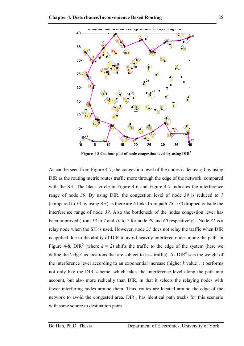
Chapter 4. Disturbance/Inconvenience Based Routing
Bo Han, Ph.D. Thesis Department of Electronics, University of York
85
Figure 4-8 Contour plot of node congestion level by using DIR2
As can be seen from Figure 4-7, the congestion level of the nodes is decreased by using
DIR as the routing metric routes traffic more through the edge of the network, compared
with the SH. The black circle in Figure 4-6 and Figure 4-7 indicates the interference
range of node 39. By using DIR, the congestion level of node 39 is reduced to 7
(compared to 13 by using SH) as there are 6 links from path 78→33 dropped outside the
interference range of node 39. Also the bottleneck of the nodes congestion level has
been improved (from 13 to 7 and 10 to 7 for node 39 and 60 respectively). Node 31 is a
relay node when the SH is used. However, node 31 does not relay the traffic when DIR
is applied due to the ability of DIR to avoid heavily interfered nodes along the path. In
Figure 4-8, DIR2 (where k = 2) shifts the traffic to the edge of the system (here we
define the ‘edge’ as locations that are subject to less traffic). As DIRk sets the weight of
the interference level according to an exponential increase (higher k value), it performs
not only like the DIR scheme, which takes the interference level along the path into
account, but also more radically than DIR, in that it selects the relaying nodes with
fewer interfering nodes around them. Thus, routes are located around the edge of the
network to avoid the congested area. DIRth has identical path tracks for this scenario
with same source to destination pairs.
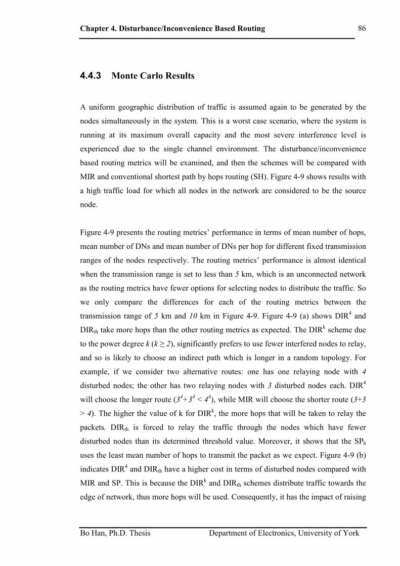
Chapter 4. Disturbance/Inconvenience Based Routing
Bo Han, Ph.D. Thesis Department of Electronics, University of York
86
4.4.3 Monte Carlo Results
A uniform geographic distribution of traffic is assumed again to be generated by the
nodes simultaneously in the system. This is a worst case scenario, where the system is
running at its maximum overall capacity and the most severe interference level is
experienced due to the single channel environment. The disturbance/inconvenience
based routing metrics will be examined, and then the schemes will be compared with
MIR and conventional shortest path by hops routing (SH). Figure 4-9 shows results with
a high traffic load for which all nodes in the network are considered to be the source
node.
Figure 4-9 presents the routing metrics’ performance in terms of mean number of hops,
mean number of DNs and mean number of DNs per hop for different fixed transmission
ranges of the nodes respectively. The routing metrics’ performance is almost identical
when the transmission range is set to less than 5 km, which is an unconnected network
as the routing metrics have fewer options for selecting nodes to distribute the traffic. So
we only compare the differences for each of the routing metrics between the
transmission range of 5 km and 10 km in Figure 4-9. Figure 4-9 (a) shows DIR4 and
DIRth take more hops than the other routing metrics as expected. The DIRk scheme due
to the power degree k (k ≥ 2), significantly prefers to use fewer interfered nodes to relay,
and so is likely to choose an indirect path which is longer in a random topology. For
example, if we consider two alternative routes: one has one relaying node with 4
disturbed nodes; the other has two relaying nodes with 3 disturbed nodes each. DIR4
will choose the longer route (34+3
4 < 4
4), while MIR will choose the shorter route (3+3
> 4). The higher the value of k for DIRk, the more hops that will be taken to relay the
packets. DIRth is forced to relay the traffic through the nodes which have fewer
disturbed nodes than its determined threshold value. Moreover, it shows that the SPh
uses the least mean number of hops to transmit the packet as we expect. Figure 4-9 (b)
indicates DIR4 and DIRth have a higher cost in terms of disturbed nodes compared with
MIR and SP. This is because the DIRk and DIRth schemes distribute traffic towards the
edge of network, thus more hops will be used. Consequently, it has the impact of raising

Chapter 4. Disturbance/Inconvenience Based Routing
Bo Han, Ph.D. Thesis Department of Electronics, University of York
87
the total number of disturbed nodes along the path from the source to the destination
node. MIR causes the least mean number of disturbed nodes in Figure 4-9 (b) as
expected because it aims to do so. In (c), DIRk and DIRth outperform MIR, SPd and SPh
in terms of minimising the number of disturbed nodes per hop. This indicates that DIRk
and DIRth routing take the individual node’s interest over the end-to-end performance.
Figure 4-9 (b) also shows that the larger the transmission range, the more nodes that are
disturbed. So there is a trade-off for choosing the transmission range. According to the
result in (a), all routing metrics have a peak value for the hop number at the
transmission range of 6 km. Moreover, this also establishes a fully connected network
with a probability of 99% in Figure 4-4. This proves that the best performance of the
network, which is used in this chapter, is achieved when nodes set the transmission
range to 6 km in the Fixed Transmission Range Scenario (FTRS).
Although MIR outperforms the other routing metrics in terms of mean number of DN,
the mean number of DN per hop can illustrate how well routing metrics can cope with
individual node/link performance rather than end-to-end performance. For example, in
cognitive radio networks, this type of routing metric can be applied amongst secondary
users as they are encouraged to relay traffic through the edge of network so that primary
users will not be interfered with by their transmissions. This can be done by modifying
the metric from taking the number of DNs to the number of primary users. Therefore,
from a per hop perspective, this implies that the fewer number of primary users per hop,
the smaller the probability that the selecting node interferes with primary users. The
routing metric design is considered to be more intelligent if it can account for individual
node/link performance. We can compare these routing metrics by calculating the
Disturbed Nodes per Hop Reduction (DNHR) at the transmission range of 6 km in
Figure 4-9 (c). The DNHR equation is shown below [52]:
DNHDNH
k
thhdDNHDNH
DN
DNHDNH
BADRDRMIRSPSPBA
AMean
BMeanAMeanDNHR
≠∈
×−
=
],,,,,[,
,100
) (
(4.23)
From the data obtained from the results in Figure 4-9 (c), at the transmission range of 6

Chapter 4. Disturbance/Inconvenience Based Routing
Bo Han, Ph.D. Thesis Department of Electronics, University of York
88
km, DIRk has an average reduction of 20% on a DN per hop basis compared with the
poorest routing metric scheme SPh, where DIRth also achieves an average reduction of
16.5%. This indicates DIRk is more focused on reducing the disturbance on a per node
basis rather than on the whole route basis.
(a) Mean number of hops vs transmission range
(b) Mean number of DN vs transmission range
(c) Mean number of DN/hop vs transmission range
Figure 4-9 Simulation results for FTRS: (a) Mean number of hops; (b) Mean number of DN; (c)
Mean number of DN/hop vs TR

Chapter 4. Disturbance/Inconvenience Based Routing
Bo Han, Ph.D. Thesis Department of Electronics, University of York
89
DIR4 performs the best out of all the routing metrics in terms of number of DNs per
hop, because DIRk is designed for picking relaying nodes that have as few disturbed
nodes as possible. This indicates DIRk is more focused on reducing the disturbance on
per node basis rather than on the whole route basis. As a result, the higher the value of
k, the fewer disturbed nodes per hop. DIRth can separate nodes to two different groups
by setting the threshold value correctly; and thus it is more robust than the other routing
metrics mentioned in this chapter. Moreover by defining the threshold value differently,
this scheme could also split nodes into more than 2 groups, providing an additional
service differentiation.
Figure 4-10 shows the performance of average congestion level versus traffic load for
each of the aforementioned routing metrics. The scenario parameters are almost the
same as in Table 4-1, except there are a variable number of source-to-destination pairs.
This has been obtained from a Monte-Carlo simulation after 1000 iterations with
source-to-destination pairs 2 to 98. The result shows that DIRk tends to have lower level
of congestion than others, especially when the traffic loads increase. This indicates that
DIRk can reduce the bottleneck of the system by reducing the network congestion level.
DIR2 can mitigate the average congestion level by 15% compared with shortest path at
high traffic load. Therefore the heavier the traffic is in the system, the more advantage
DIRk can deliver to improve the end-to-end congestion level. This is because DIR only
reduces the interference on a whole path basis, irrespective of which individual nodes
are selected for relaying the traffic. By changing the k value of the routing metric, it has
the ability to alter routes through the network in response to the interference or
congestion.

Chapter 4. Disturbance/Inconvenience Based Routing
Bo Han, Ph.D. Thesis Department of Electronics, University of York
90
Figure 4-10 Average congestion level against traffic load measured in number of active source
destination pairs
4.5 Conclusion
This chapter shows the early work of designing a family of routing metrics to avoid
congested areas. Disturbance/Inconvenience based routing metric (DIR) takes both
outward and inward interference into routing metric design. The extensions of DIR
(DIRk and DIRth) have the ability to adjust their link weight so that they can take
individual node states into account as well as the end-to-end perspective. DIRk can treat
the interference on the same node/link differently by adjusting the link/node weight to
the power of k. By changing the k value, DIRk is able to decide to select intermediate
nodes which provide the lowest interference on an end-to-end basis or individual basis
due to the exponential impact on links/nodes weight. DIRth separates links/nodes into
two groups due to the interference threshold value.
There are still many limitations of this DIR routing metric design. For example, the
routing metric cannot adapt well to environment changes as it only takes disturbed node
number into account, regardless of traffic flows, bottleneck nodes and channel
assignment etc. In addition, DIR selects routes by going through nodes with fewer DN.
This characteristic results in unnecessary hops which lead to extra relaying burdens on
the whole network. Therefore, it is recommended to apply DIR in a network scenario

Chapter 4. Disturbance/Inconvenience Based Routing
Bo Han, Ph.D. Thesis Department of Electronics, University of York
91
where traffic load is relatively low or there is sufficient radio spectrum to fulfil the
traffic demand, so that it can route around congested areas without limiting network
capacities due to extra relaying hops. More sophisticated routing metric designs will be
shown in later chapters.

Chapter 5. Routing Metric Design to Improve End-to-end Bottleneck Capacity
Bo Han, Ph.D. Thesis Department of Electronics, University of York
92
Chapter 5
5 Routing Metric Design to Improve End-
to-end Bottleneck Capacity
Contents _____________________________________________________________________
5 Routing Metric Design to Improve End-to-end Bottleneck Capacity.....................92
5.1 Introduction .....................................................................................................92
5.2 Capacity Model ...............................................................................................93
5.2.1 Node Capacity .........................................................................................94
5.2.2 Node Virtual Capacity.............................................................................94
5.3 Capacity Based Routing ..................................................................................95
5.4 Bottleneck-aware Routing...............................................................................97
5.4.1 Routing Metric Design ............................................................................98
5.5 Network and Traffic Model.............................................................................99
5.6 Performance ..................................................................................................100
5.7 Conclusion.....................................................................................................105
_____________________________________________________________________
5.1 Introduction
One advantage of a wireless ad hoc network is its multi-hop feature as nodes can
forward packets from source to destination on a hop-by-hop basis. However, relaying
can reduce network capacity as nodes contend for capacity not only with others serving
on routes nearby, but also with those nodes taking part in relaying on the same path.
The capacity of an ad hoc network can be surprisingly low due to these inter-flow and
intra-flow contentions [30].

Chapter 5. Routing Metric Design to Improve End-to-end Bottleneck Capacity
Bo Han, Ph.D. Thesis Department of Electronics, University of York
93
In the previous chapter, we presented the early work of routing metric design by taking
the number of disturbed nodes into account to avoid congested areas. However, this
routing metric design cannot cope well with environmental changes due to traffic flows
and varying link/node capacities. For example, a route that is selected to go through a
node with low capacity may result in a longer delay or lower throughput even when
other nodes along the path may have sufficient capacity. Therefore, it is desirable to
find a routing metric design that can not only improve the overall network capacities but
also avoid creating bottleneck nodes in wireless ad hoc networks.
The purpose of this chapter is to design a routing metric, which is referred to as
bottleneck-aware routing (BAR), that takes the current node capacity into account as
well as the bottleneck node location to improve the bottleneck capacity in a
heterogeneous ad hoc network. It is inspired by capacity based-routing [53] which
incorporates the node capacity into the routing metric design in order to improve the
capacity of the wireless ad hoc networks.
The details of the capacity model used are given in section 5.2. Then, section 5.3
reviews capacity-based routing (CBR), which is followed by the proposed bottleneck-
aware routing (BAR) metric design in section 5.4. Section 5.5 outlines the network
scenario which is used in this chapter. Comparative simulation and analytical results are
presented for BAR, CBR and shortest path by hops (SH) in section 5.6. Finally we will
draw the conclusions in section 5.7.
5.2 Capacity Model
In this section, the capacity model is defined to include node capacity and node virtual
capacity.

Chapter 5. Routing Metric Design to Improve End-to-end Bottleneck Capacity
Bo Han, Ph.D. Thesis Department of Electronics, University of York
94
5.2.1 Node Capacity
In this chapter, a heterogeneous network with 3 different types of node (basic node,
aggregation node and landmark node) is used.
• Basic nodes have lowest capability for transmitting data with low bandwidth
ranges from 100 Kbps to 1 Mbps (e.g. sensor nodes in wireless sensor networks)
• Aggregation nodes have medium capability for transmitting data. These nodes
are responsible for aggregating traffic from multiple low capability nodes and
have medium bandwidth from 1 Mbps to 2 Mbps (e.g. cluster head)
• Landmark nodes have a high capacity for transmitting data with high bandwidth
from 2 Mbps to 4 Mbps. Those nodes can operate with advanced techniques (e.g.
directional antenna) that will handle trunked traffic for communicating directly
with the high-speed infrastructures such as a headquarter in a battlefield
The node capacity (C) is determined by their node types. Network capacity can be
improved by better exploiting the network hierarchies of ad hoc networks [53].
5.2.2 Node Virtual Capacity
The virtual capacity of a node (CV) is introduced here as the capacity allocated to the
link for a specific routing. It is a portion of the raw capacity of the node (CV ∈ C) and it
is determined by the co-channel interference (node congestion level which has been
defined in the previous chapter). We assume fair scheduling TDMA is used so that each
link that competes for the same channel can be assigned a different time slot with an
equal length. This scenario implies that the route has to share the bandwidth not only
with routes going through the node of interest, but that it also has to share the bandwidth
with the routes going through the interferers of the node of interest. Therefore, the
virtual capacity of node N0 is the raw capacity of the channel divided by the congestion
level for its routing task. For example, Figure 5-1 shows that the virtual capacity of
node N0 is C / 8 as there are 8 links going through the interference range of N0 , and the
raw capacity is then evenly divided for each transmission as shown in Figure 5-2.

Chapter 5. Routing Metric Design to Improve End-to-end Bottleneck Capacity
Bo Han, Ph.D. Thesis Department of Electronics, University of York
95
Figure 5-1 Example of traffic through the network
Figure 5-2 Capacity usage at N0, including usage by interference links.
5.3 Capacity Based Routing
In heterogeneous networks, nodes have different sending rates, transmit powers and
antenna gains. These factors result in a different capacity in each direction on a link.
Traditional ad hoc routing metrics, like shortest path, cannot take these different link
capacities into account. Higher capacity links might remain unused and lower capacity
links might end up being crowded. As a result, it is crucial for an ad hoc network to
relay more traffic through the higher capacity links to improve load balancing. Figure
5-3 demonstrates an example where the use of a longer route in terms of hop number
could be desirable due to the preferable link capacity on the route.

Chapter 5. Routing Metric Design to Improve End-to-end Bottleneck Capacity
Bo Han, Ph.D. Thesis Department of Electronics, University of York
96
Figure 5-3 Routing from A to D. The dotted route is preferred due to the link capacity is higher on
this route.
It is desirable to shift the traffic from a lower capacity node to those which are more
capable to relay. Since the capacity in this chapter is mainly determined by active traffic
interactions (intra-flow and inter-flow interference), capacity-based routing (CBR) can
divert the upcoming traffic to an uncongested area in order to make the whole network
more scalable. Here we recall the CBR metric which is shown in Chapter 2, as the link
weight of CBR is defined by [53]:
VjiC
wjv
ij ∈∀= ,,1
_
(5.1)
Where wij indicates the weight value of the link (from node i to node j), and Cv_j
indicates the virtual capacity of node j. The virtual capacity of node j is determined by
the maximum capacity of the node (check Table 5-1 for each node type) divided by the
congestion level this node suffers:
j
j
jvCL
MbpsBC
)(_ =
(5.2)
By using Dijkstra's algorithm, CBR prefers to select nodes with higher capacities, with
routes established based on the maximisation of the accumulated impact capacity on an
end-to-end basis.
A
B C
D
E

Chapter 5. Routing Metric Design to Improve End-to-end Bottleneck Capacity
Bo Han, Ph.D. Thesis Department of Electronics, University of York
97
End-to-end bottleneck capacity, introduced in Chapter 3, is constrained by the minimum
capacity value along the path. If the node upstream of the bottleneck node injects more
packets into the link than the bottleneck node can forward. Thus delay will increase as
packets get stuck at the bottleneck and throughput reduces as these packets are
eventually dropped by the congested node. Therefore, it is important for routing metric
design to be aware of the bottlenecks and if possible, relay traffic by avoiding the
bottleneck nodes as well as nodes nearby them due to the possibility of co-channel
interference.
5.4 Bottleneck-aware Routing
Since the bottlenecks are a limitation to the end-to-end performance, routing metrics
should take the impact of the bottleneck node into account when selecting routes. There
are other routing metrics that have been carried out to improve capacity, load balancing,
and hotspot problems such as capacity-based routing (CBR) [53], DLAR [65] and HMP
[66]. Liu’s capacity-based routing [53] aims to improve network capacity by selecting
links with higher capacity on an end-to-end basis without accounting for the impact on
the network caused by individual bottleneck links. Lee and Gerla demonstrated a
dynamic load-aware routing algorithm (DLAR) [65] which considers the traffic load of
the intermediate nodes as the main route selection criterion. DLAR focuses on selecting
routes that have the least number of intermediate nodes that have packets buffered by
more than a threshold value. This scheme neglects inter-flow interference as in practice
the traffic that relays through the nearby nodes can also increase the severity of the
bottlenecks. Lee and Campbell presented a hotspot mitigation protocol (HMP) [66]
where hotspots represent transient but highly congested regions in wireless ad hoc
networks. This solution focuses on alleviating the congested area but fails to take the
individual bottlenecks into account. To the best of our knowledge, there are no
comprehensive studies and good solutions for routing metrics for scenarios where there
is a wide variety of node types and capabilities (e.g. low, medium and high capacity
nodes), that also optimise end-to-end performance, by taking into account local area
based congestion.

Chapter 5. Routing Metric Design to Improve End-to-end Bottleneck Capacity
Bo Han, Ph.D. Thesis Department of Electronics, University of York
98
5.4.1 Routing Metric Design
In this section, the routing metric design of BAR is provided. Bottleneck-aware routing
(BAR) selects nodes that have a maximum capacity value on a multi-hop transmission
path in a similar manner to CBR, but also routes around any bottlenecks. Here the link
weight of BAR is defined as:
VjiwBNj
C
BNjC
ijj
j
∈∀
=∉
∈+,,
,1
,1
δ
(5.3)
Where BN is a set that contains the end-to-end bottleneck nodes of each traffic flow and
nodes within the interference range of those end-to-end bottleneck nodes, and δ is a
punishment value. If the node is not one of the bottlenecks or the interferer of a
bottleneck, the weight remains the same as with CBR. If however the node is either one
of the bottlenecks or their interferers, the weight is increased as a punishment by a value
δ. The assumption is made here that the interferer node can be informed by the
bottleneck node. The discussion of how this is done is beyond the scope of this thesis.
The routing protocol associated with the bottleneck-aware routing metric design will be
given in the following section to help each node be aware of the other’s capacity as well
as the locations of end-to-end bottleneck nodes. The bottleneck-aware routing metric is
monotonic as weight values are all positive and it is isotonic due to the fact that the
subsequent path choice does not affect the weight value of the predecessor path since
the current path is calculated and selected based on the weight value of each link from
the previous event.
For the scenario here a punishment value of 7 is chosen as this is the average number of
nodes within 1 hop distance. The calculation is based on equation (4.6) in Chapter 4 and
the network parameters can also be found later within this chapter. There is a trade-off
between the punishment values. If the value is too small, routes cannot be fully alerted
to avoid going through the congested areas, but if it is too large, it could cause
significant relaying, potentially deteriorating future traffic demands.

Chapter 5. Routing Metric Design to Improve End-to-end Bottleneck Capacity
Bo Han, Ph.D. Thesis Department of Electronics, University of York
99
5.5 Network and Traffic Model
The proposed routing metric will be examined in a 10-by-10 grid network environment.
There are three different types of nodes in this network: landmark nodes, aggregation
nodes and basic nodes. The key parameters are shown in Table 5-1. This is a fully
connected scenario. Nodes that have the least number of potential connecting links are
located in the corners, where they have just 2 neighbours, with nodes in the middle
having the most connections with 4 neighbours. We assume routes do not change during
their life-time once they are established. This is convenient for nodes to sense the states
of the network and to reduce the route oscillation problem [67].
Key parameters Value
Network size 40 × 40 m2
Number of nodes 100
Number of landmark nodes 20
Number of aggregation nodes 20
Number of basic nodes 60
Node’s transmission range 6 m
Node’s interference range 12 m
Capacity of landmark link 4 Mbps
Capacity of aggregation link 2 Mbps
Capacity of basic link 1 Mbps
Mean duration of each
connection per source node
0.2 seconds
Inter-arrival distribution range
per source node
0.25 to 6
arrivals/seconds
Table 5-1 Parameter values used in the example scenario
This is a call based ON-OFF traffic model. The mean arrival and the mean duration of
each route connection follow a Poisson distribution. All traffic originates at the left
edges of the grid network and is forwarded to the right edge. The middle nodes do not
originate any traffic. The sources and destinations are selected on each edge of the

Chapter 5. Routing Metric Design to Improve End-to-end Bottleneck Capacity
Bo Han, Ph.D. Thesis Department of Electronics, University of York
100
network as we want to analyse the multi-hop relaying characteristic of each routing
metric across the network. Aggregation nodes are selected randomly in the middle. The
traffic model in this chapter is more realistic than the traffic model used in the previous
chapter. In the previous chapter, once a route connection is established, it remains in the
network until the simulation finishes. In this chapter, the arrival and duration of traffic
flows have negative exponential distribution. A flow will arrive at each source 10 times
during the simulation time. The routing metrics are examined on an event basis. An
event occurs when an end-to-end traffic flow is established (ON) or deactivated (OFF)
in the network. The maximum number of concurrent routes that can be in operation at a
single time is 10.
5.6 Performance
In this section, we examine the effectiveness of different routing mechanisms among
shortest-path by hops (SH), capacity based routing (CBR) and bottleneck-aware routing
(BAR). Firstly, an example of a snapshot scenario is given to show the improvement in
end-to-end bottleneck capacity by using BAR, compared with SH in Figure 5-4 and
Figure 5-5. Figure 5-6 shows the CDF of end-to-end bottleneck capacity with different
routing metrics at an average traffic load of 3 traffic flows. The comparative
performance of end-to-end bottleneck capacity against traffic load will be shown in
Figure 5-7.
Figure 5-4 and Figure 5-5 show each node’s average congested levels for SH and BAR
routing metrics respectively.
• A circle indicates node congestion level, the bigger the circle, the more
congestion this node is suffered
• Dark lines illustrate the concurrent traffic flows in the network
• Dots in the middle are the end-to-end bottleneck nodes due to their node
capacity and traffic locations

Chapter 5. Routing Metric Design to Improve End-to-end Bottleneck Capacity
Bo Han, Ph.D. Thesis Department of Electronics, University of York
101
• A cross indicates an aggregation node
In Figure 5-4, SH illustrates that nodes in the middle become very congested as
expected, due to the traffic patterns that are generated across the network from left to
right, given that SH only selects paths with minimum hop count. This is the worst case
for load balancing which leads nodes in the middle of the network to become
bottlenecks, with capacity being wasted around the edge.
On the other hand, BAR finds the path by exploiting the highest capacity nodes to relay
the traffic, and more importantly, BAR routes around bottleneck links. This improves
the load balancing as can be seen in Figure 5-5, where the general number and levels of
bottlenecks are reduced by the BAR routing metrics in comparison with SH. The
capacity is designed to take intra-flow and inter-flow interference into account. BAR
maximises the possibility to improve the network throughput by allowing concurrent
transmissions. Flows are shifted from the middle to the edges of the network.
The graph of CBR, which shows the average congestion level of each node during the
simulation time, looks similar to Figure 5-5 as BAR is designed based on CBR.
Therefore, we will not show the congestion level graph of CBR.

Chapter 5. Routing Metric Design to Improve End-to-end Bottleneck Capacity
Bo Han, Ph.D. Thesis Department of Electronics, University of York
102
Figure 5-4 Snapshot of node congestion level by using shortest path routing metrics
Figure 5-5 Snapshot of node congestion level by using BAR
Earlier, we discussed how the bottleneck capacity of nodes can jeopardize the

Chapter 5. Routing Metric Design to Improve End-to-end Bottleneck Capacity
Bo Han, Ph.D. Thesis Department of Electronics, University of York
103
performance not only on a specific traffic flow, but also the capacity of the whole ad
hoc network. It is crucial to try and reduce the number of bottlenecks and increase the
bottleneck capacities. Figure 5-6 shows the benefit of reducing the bottlenecks using
BAR routing metrics. In this figure, the horizontal dot line indicates the 90th percentile
of each figure. Due to the bottleneck aware feature, 90% of the bottlenecks have a node
virtual capacity value of about 110 kbps (as the point on the x-axis where a vertical line
intersects the BAR curve on 90th percentile), about 75 kbps (as the point on the x-axis
where a vertical line intersects the CAR curve on 90th percentile) and about 63 kbps (as
the point on the x-axis where a horizontal line intersects the SH curve on 90th percentile)
by using BAR, CBR and SH respectively. At this percentile, BAR shows a significant
improvement on increasing bottleneck capacity by 31.8% and 42.7% higher than SH
and CBR respectively.
Figure 5-6 CDF of long-term end-to-end bottleneck capacity with different routing metrics
Figure 5-7 shows the sum of the bottleneck capacities on each active route against
different traffic loads respectively. The minimum node/link capacity along a path is
considered to the bottleneck and all routes only have a single bottleneck. The reason of
using the total bottleneck capacity as a metric instead of the mean value is because the
bottleneck capacity is the minimum capacity along the path and it is very small value.
The bottleneck capacity depends on the network topology, node capacity, traffic pattern
and routing metric. Although the routing metric is different, the other conditions are

Chapter 5. Routing Metric Design to Improve End-to-end Bottleneck Capacity
Bo Han, Ph.D. Thesis Department of Electronics, University of York
104
completely identical when applying different routing metrics. In Figure 5-7, bottleneck
capacity is only determined by the applied routing metric, which cannot provide
significant variations among different routing metrics if the mean bottleneck capacity
was used. The total value can illustrate the maximum variation on the bottleneck
capacity by comparing different routing metrics.
At light traffic load levels, the network has enough capacity for traffic relaying.
Therefore, the BAR can route around bottleneck nodes by using extra hops or relaying
without reducing the capacity of the network. It can be seen in Figure 5-7 for example
that BAR improves the whole network bottleneck capacity by 60% and 14% at an
average traffic load of 4 traffic flows compared with SH and CBR respectively. At this
traffic load, BAR can efficiently separate nodes or links into different classes. However,
at heavy traffic load levels, CBR and especially BAR will reduce the network capacity
due to their routing characteristic which attempts to avoid congested areas which could
generate an extra relaying burden for the network. Moreover, the extra relaying
competes for channel capacity not only with originated traffic but also with other
relaying nodes. This competition for the channel capacity generates more bottleneck
nodes and reduces the capacity of the network. We will show more details in the
following chapters.
Figure 5-7 Summation of end-to-end bottleneck capacity against traffic loads

Chapter 5. Routing Metric Design to Improve End-to-end Bottleneck Capacity
Bo Han, Ph.D. Thesis Department of Electronics, University of York
105
5.7 Conclusion
In this chapter, we proposed a novel routing metric design, Bottleneck-Aware Routing
(BAR), which can improve the end-to-end bottleneck capacity in a relatively low traffic
load network. The constraints of CBR and BAR have also been discussed.
BAR is considered to be more intelligent than shortest-path by hops (SH) and
disturbance/inconvenience based routing (DIR) as it accounts for individual node/link
capacity which is related to current traffic flows in its metric design. BAR not only
takes individual node’s interference and capacity into account like CBR but also is
aware of the location of bottleneck nodes such that paths can intelligently pick the high
capacity nodes to forward packets and also route around bottleneck nodes. Under low
traffic loads, results show that BAR can improve end-to-end bottleneck capacity
significantly compared with SH and CBR.

Chapter 6. Exploiting Cross-layer Design for Wireless Ad Hoc Networks
Bo Han, Ph.D. Thesis Department of Electronics, University of York
106
Chapter 6
6 Exploiting Cross-layer Design for
Wireless Ad Hoc Networks
Contents _____________________________________________________________________
6 Exploiting Cross-layer Design for Wireless Ad Hoc Networks ...........................106
6.1 Introduction ...................................................................................................106
6.2 Cognitive Greedy-backhaul Routing.............................................................108
6.3 Simple Channel Assignment Scheme ...........................................................111
6.3.1 Random Scheme....................................................................................112
6.3.2 Quasi-fair Scheme .................................................................................113
6.4 Network Model .............................................................................................113
6.4.1 Capacity and Throughput ......................................................................113
6.4.2 Parameters .............................................................................................116
6.5 Results ...........................................................................................................117
6.6 Conclusions ...................................................................................................120
_____________________________________________________________________
6.1 Introduction
One of the most important features of wireless ad hoc networks is their decentralized
character, with nodes that can function as routers, fulfilling not only their own traffic
demands, but also forwarding the packets of others (relaying). This feature helps node
transmissions to reach their destination through multi-hop relaying. It also places
constraints on ad hoc networks, due to the competition for the limited frequency
spectrum between relaying and originated traffic as well as between relaying traffic

Chapter 6. Exploiting Cross-layer Design for Wireless Ad Hoc Networks
Bo Han, Ph.D. Thesis Department of Electronics, University of York
107
from different sources. In addition, this relaying burden on the network reduces per
node throughput, as shown in [12], the throughput per node shrinks in scaled length as
)/1( nO . The relaying burden is generated since nodes have to spend their
transmission time sending the data of other nodes [68]. The relaying burden on
intermediate nodes has been considered as one of the main capacity constraints in
wireless ad hoc networks. Therefore, unnecessary relaying/hops should be minimised
for route selection.
In wireless ad hoc networks, the selection of suitable intermediate nodes for relaying
traffic is crucial and will influence future traffic. The traditional wireless ad hoc
network routing metric is shortest path by hops (SH), which selects routes using the
criterion of minimum hop count. This is the simplest routing metric and it has the
lowest relaying burden impact on the network. However, SH is not aware of any
network conditions such as capacity, energy consumption, throughput etc and it tends to
cause congestion problems by leading traffic flows to specific locations. Other routing
metrics e.g. DIR, BAR and CBR as shown in the previous chapters, can take
interference, bottleneck and capacity into their routing metric designs in order to move
routes from a congested area to one less crowded. However, the relaying burden rises
due to an increased number of hops around the network. Those routing metrics reduce
the network capacity even further in the scenario where channels are inadequate to
satisfy the relatively high traffic demand as they generate extra hops. Unnecessary
relaying hops creates more severe competition on the limited frequency spectrum and
results in producing more bottlenecks.
Since it is a big challenge for wireless ad hoc routing metric design to solve the trade-
off problem between relaying burden and bottlenecks, in this chapter we will introduce
a cross-layer design to minimise the relaying impact on the network without
deteriorating the end-to-end quality of service. The cross-layer scheme is associated
with a novel routing metric design ‘Cognitive Greedy-Backhaul (CGB)’ with a channel
assignment scheme. It aims to create cognitive backhaul links which can reduce the
relaying burden and alleviate the bottleneck problem. In this thesis, we refer to backhaul
links as links with higher capacities and which are subject to a high traffic demand due

Chapter 6. Exploiting Cross-layer Design for Wireless Ad Hoc Networks
Bo Han, Ph.D. Thesis Department of Electronics, University of York
108
to their important geographical locations. In other words, backhaul links are created in
congested areas with higher capacity.
Unlike other routing metrics that exploit the spatial-temporal diversity to improve the
spatial reuse/capacity of the network, CGB forces routes to go through nodes/links/areas
with naturally important geographical locations which generate a relatively low relaying
impact on the network. These crowded links can provide extra capacity if an appropriate
channel assignment scheme is applied. In other words, a bottleneck problem can be
alleviated if we can assign more channels/capacities intelligently to the places where
they are needed. A couple of simple channel assignment schemes are initially applied to
understand how the cross-layer design and CGB function in wireless ad hoc networks.
This chapter is structured as follows. Section 6.2 and 6.3 outline the cognitive greedy-
backhaul routing and simple channel assignment schemes respectively to be used in the
cross-layer design. In section 6.4, we introduce our network model. In addition, we
compare the proposed CGB routing metric with shortest path by hops (SH) and
Capacity-Based Routing (CBR) by presenting simulation results in section 6.5. Finally,
the conclusions are drawn in section 6.6.
6.2 Cognitive Greedy-backhaul Routing
CGB aims to create cognitive backhaul links by exploring network conditions, traffic
demand and channel usage. It requires the routing metric to exploit environmental
information sensed by nodes and for them to adapt their weighting factors to indirectly
improve the end-to-end performance of the whole network.
In this chapter, multiple channels are used in the network instead of the single channel
scenario applied in previous chapters, and links can occupy more than 1 channel for
their data transmission. In this thesis, the number of channels required for a link is
determined by the number of different originated traffic flows flowing through the link.
This is to make sure wireless ad hoc network capacity can still be maintained for
nodes/links with important locations to avoid becoming bottlenecks when a suitable

Chapter 6. Exploiting Cross-layer Design for Wireless Ad Hoc Networks
Bo Han, Ph.D. Thesis Department of Electronics, University of York
109
channel assignment scheme is applied. For example, Figure 6-1 shows that link ℓ
requires 3 channels to transmit data from source node S1, S2 and S3 without becoming
a bottleneck link. Thus, we say that link ℓ has the channel utilization level of 3 as three
different originated traffic flows (from S1, S2 and S3) are required to go through the
link. To enable transmissions to be simultaneously operated not only between the
intermediate links on the same flow path but also between links on a different flow path,
a good channel assignment scheme has to be applied with CGB to avoid intra-flow and
inter-flow interference.
Figure 6-1 Channel usage example
Earlier, we commented that one of the main capacity constraints of wireless ad hoc
networks is caused by the relaying burden. From a wireless ad hoc routing perspective,
the extra relaying burden is generated from unnecessary relay hops. Traditional wireless
ad hoc routing metrics cannot solve this problem. Cognitive greedy-backhaul routing
(CGB) selects links based on their utilization level, which we define as the number of
source-to-destination pairs that are required to go through the link. CGB relays traffic
flow through crowded links due to their important geographical location. Those routes
are constructed based on their important geographical location which leads to a
minimum hop scheme from source to destination. With a proper channel assignment
scheme, additional capacity can be allocated to those crowded links and backhaul links
can be established. The relaying burden and bottlenecks are improved by attracting
traffic through those backhaul links.
D
S3
S2
S1
ℓ

Chapter 6. Exploiting Cross-layer Design for Wireless Ad Hoc Networks
Bo Han, Ph.D. Thesis Department of Electronics, University of York
110
Figure 6-2 illustrates how CGB functions. Initially, CGB selects the route as the shortest
path by hops (SH) in Figure 6-2 (a). Based on the traffic requirement and geographic
location, heavily used nodes/links can be distinguished. Then, those links attract more
traffic flow due to their lower weight values. Link capacity is maintained by assigning
more channels to fulfil different traffic flows as shown in Figure 6-2 (b). Finally, more
upcoming traffic will flow through the backhaul links due to their lower weight value as
shown in Figure 6-2 (c). In contrast, some routing metric designs have been proposed to
overcome the bottleneck problem by diverting around crowded areas such as a hotspot
mitigation protocol (HMP) [66] and bottleneck-aware routing (BAR). Those diverting
routes increase the relaying burden due to the longer distance/greater number of hops
taken as they route around congested areas or bottleneck nodes/links. Therefore, in the
scenario where traffic load is relatively high with respect to channel capacity, those
routing metrics potentially create even more bottlenecks and congested areas.
CGB forwards nodes with a high channel utilization level (number of channels
occupied). Here the link weight of CGB is defined as:
VjiPUU
w ij
ij
ij ∈∀≤= ,|,|,1
(6.1)
Uij indicates the utilization level of the link ij which is equal to the number of end-to-
end traffic flows through the link. In other words, Uij also equals the number of
channels that are required for link ij due to the assumption we made that the number of
channels required for a link is equal to the number of different end-to-end traffic flows
through the link in order to avoid the bottleneck node problem. P and |P| are the set that
contains the channels, and the number of channels that can be used in the network,
respectively.
The link weight is positive which proves the routing metric is monotonic. In addition,
the link weight is determined by the number of traffic flows through the link at the
previous event. Therefore, the subsequent choice of path will not affect the weight value
of the predecessor path as the number of traffic flows through the object link is already

Chapter 6. Exploiting Cross-layer Design for Wireless Ad Hoc Networks
Bo Han, Ph.D. Thesis Department of Electronics, University of York
111
determined at the last event. This shows the CGB routing metric is isotonic. More
details about routing isotonicity and monotonicity can be found back in Chapter 2.
CGB prefers to pick nodes/links which have more occupied channels. This means the
higher the channel utilization level of a node/link, the more likely it is that CGB will
select it for future traffic flows, thus cognitive backhaul links are established. CGB
builds cognitive backhaul links by exploring the traffic conditions and important
geographic location of nodes; it can occupy more channels, delivering higher capacity
where a high level of traffic is required. Therefore the bottleneck problem is reduced by
using a backhaul which can obtain more capacity if needed.
Figure 6-2 Shows how CGB performs (a) initial function as SH by same weight value of 1, (b)
weight value reduces due to the usage, (c) backhaul links established due to the important
geographical locations; solid arrows indicate CGB path; dotted arrows show the possible route
selection by shortest path
6.3 Simple Channel Assignment Scheme
To illustrate the benefits of using the cognitive greedy-backhaul algorithm, the network
needs to operate in a multi-channel environment. Therefore we apply two simple

Chapter 6. Exploiting Cross-layer Design for Wireless Ad Hoc Networks
Bo Han, Ph.D. Thesis Department of Electronics, University of York
112
channel assignment schemes to start with to understand how this cross-layer design can
achieve end-to-end goals in wireless ad hoc networks. More advanced channel
assignment schemes will be applied with CGB to analyse the cross-layer design impact
it will have on the practical wireless ad hoc network scenario in the next chapter.
The cognitive greedy-backhaul routing metric has the ability to force traffic flows to
form concentrated backhaul links. In order to reduce the bottleneck problem, we need to
consider the cross-layer design and assign more channels (capacity) to the backhaul
links as needed. Due to the focus on routing metric design in this chapter, we therefore
introduce two relatively basic channel assignment schemes for the benefit of illustrating
this novel routing metric design. To simplify the channel assignment scheme in this
chapter, the same channel is assigned to an entire end-to-end traffic flow. In other words,
assuming an appropriate channel assignment scheme is used and there are sufficient
channels, we only need to consider the intra-flow rather than inter-flow interference and
resource sharing. In the case where there are insufficient channels for this to occur,
capacities are equally divided by intra-flow and inter-flow interference. The point of
illustrating these two channel assignment schemes is to show how the cognitive greedy-
backhaul routing metric can performs better with a better channel assignment scheme
than a poor one. In the next chapter, we will elaborate on how well CGB can be
associated with a reinforcement learning based channel assignment scheme.
6.3.1 Random Scheme
A random channel assignment scheme assigns channels from a spectrum pool randomly
to a new traffic flow without considering spatial reuse and fairness. We assign a random
channel },..,3,2,1{ px i ∈ to each new end-to-end traffic flow, where p is the number of
channels available in the network.

Chapter 6. Exploiting Cross-layer Design for Wireless Ad Hoc Networks
Bo Han, Ph.D. Thesis Department of Electronics, University of York
113
6.3.2 Quasi-fair Scheme
The quasi-fair channel assignment scheme assigns channels from a spectrum pool
corresponding to current channel utilization in the network. The least utilized channels
(up) are selected for new traffic flows that arrive in the network rather than using the
channels that have already been allocated to the existing traffic flows. Each source node
sends HELLO packets that include the channel it occupies periodically on all channels.
Nodes receive the HELLO packets from source nodes and can determine the utilized
value of each channel and make a decision about which channel is assigned in the link
layer. For example, if there are 3 channels ( }3,2,1{∈ix ) available and 5 concurrent
traffic flows in the network. If channels 1, 2 and 3 are assigned to traffic flows twice (u1
= 2), twice (u2 = 2) and once (u3 = 1) respectively, then channel 3 will be allocated to
the 6th concurrent traffic flow. This is because u3 is the lowest utilized value compared
with the other channels. The quasi-fair scheme is more ‘intelligent’ than the random
scheme as it takes current channel utilization into account. It is a centralised channel
assignment scheme which operates in an opposite way to a distributed scheme. This
shows that with a better channel assignment scheme, the cross-layer design can deliver
better results. In the next chapter, channels are assigned in a distributed way for all
channel assignment schemes.
6.4 Network Model
In this section, we introduce our network model which includes the main performance
factors: end-to-end throughput and available capacity.
6.4.1 Capacity and Throughput
In contrast to the capacity model we introduced in the previous chapter, we use a multi-
channel model to examine how well the greedy routing metric can cope in a multi-
channel scenario. The available capacity (Ca) is determined by the summation of the
remaining capacity (Cr) on each channel. We assume nodes have the same transmit

Chapter 6. Exploiting Cross-layer Design for Wireless Ad Hoc Networks
Bo Han, Ph.D. Thesis Department of Electronics, University of York
114
power, therefore the remaining capacity (Cr) of channel k for the objective node j is only
defined by the intra-flow and inter-flow interference on channel k within the
interference range of node j and maximum channel capacity (Ck_m) is:
PkVjCL
CC
kj
mk
kjr ∈∀∈∀+
= ,,1_
_
_,
(6.2)
Where V and P are the set of nodes and channels in the network respectively. Ck_m is the
maximum capacity that can be achieved by channel k, which is 20 Mbit/s in this chapter
for all channels. CLj_k is the congestion level of node j on channel k. The congestion
level of node j on channel k is defined as:
VjRCL ji
NI
jikj
j
∈∀∑==
,_0_
_
(6.3)
Where NIj is the number of nodes within the interference range of node j, and Ri_j is the
number of routes going through node i_j, which is one of the interferers of node j, using
channel k. R0_j indicates the number of routes going through the node of interest. For
example, we can see from Figure 6-3 that the congestion level of objective node N0 by
using channel 3 is 6 active links which includes all intra-flow and inter-flow
interference. This indicates that each activated link which uses the same channel shares
the same amount of bandwidth to fulfil their transmissions.
The available capacity of node j is defined as:
VjCC jr
P
jrja ∈∀∑=
=,_
||
1__
(6.4)
Where |P| is the number of channels that can be used for the network, Cr_j is the
remaining capacity of node j by using channel r_j which is one of the channels in the
network. In Figure 6-3, there are three channels in the network. The remaining
capacities of node N0 for channel 1, 2 and 3 are 5 Mbps, 4 Mbps and 2.5 Mbps
respectively. Thus the available capacity of node N0 is 11.5 Mbps. This implies that the

Chapter 6. Exploiting Cross-layer Design for Wireless Ad Hoc Networks
Bo Han, Ph.D. Thesis Department of Electronics, University of York
115
route has to share the bandwidth not only with routes going through the node of interest,
but also with the routes going through the interferers of the objective node.
In the previous chapter, we investigated capacity based routing (CBR) in a single
channel scenario. Here, available capacity-aware routing (AC) is proposed for multi-
channel scenario. The available capacity-aware routing algorithm is based on the
maximization of the accumulated impact available capacity has on multi-hop
communication. The link weight of AC is defined as:
VjiC
wja
ij ∈∀= ,,1
_
(6.5)
Figure 6-3 Example of traffic flows through the network
The throughput of node j is defined as:
VjCL
CS
kch
mkchNC
kchj ∈∀
+∑==
,1_
,_
1_
η
(6.6)
Where η indicates a MAC efficiency factor; NC is the number of channels that have
been utilised by node j; Cch_k,m is the maximum capacity of channel ch_k and CLch_k is
the congestion level of node j on channel ch_k.
N0
CH [1]
CH [2]
CH [3]
CH [3]

Chapter 6. Exploiting Cross-layer Design for Wireless Ad Hoc Networks
Bo Han, Ph.D. Thesis Department of Electronics, University of York
116
Evaluating end-to-end bottleneck throughput is our main method of evaluating the
performance of the combined routing metrics and channel assignment schemes. It is
constrained by the minimum throughput value along the path, i.e. it occurs when the
upstream node of the bottleneck node injects more packets into the link than the
bottleneck node can forward. End-to-end delay increases as packets get stuck at the
bottleneck and the throughput reduces as these packets are eventually blocked by the
congested node.
6.4.2 Parameters
In this chapter, we assume a wireless ad hoc network where nodes are in a fixed
location without mobility. The aforementioned routing metrics will be examined in a
randomly located node environment. There are 99 source nodes and 1 sink node, located
randomly in the network. The key parameters are shown in Table 6-1. This is a fully
connected scenario. We assume routes do not change during their life-time once they
are established. This is convenient for nodes to sense the state of the network and to
reduce the route oscillation problem [67].
Key parameters Value
Network size 40 × 40 m2
Number of nodes 100
Number of source nodes 99
Number of sink node 1
Number of channels 10
Node’s transmission range 7 m
Node’s interference range 14 m
Maximum channel capacity 20 Mbps
Mean duration of each
connection per source node
0.2 seconds
Inter-arrival distribution range
per source node
0.25 to 6
arrivals/second
Table 6-1 Parameter values used in the example scenario
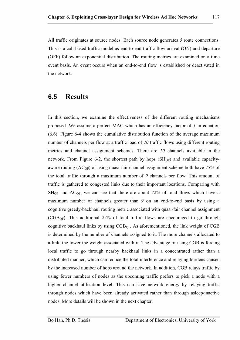
Chapter 6. Exploiting Cross-layer Design for Wireless Ad Hoc Networks
Bo Han, Ph.D. Thesis Department of Electronics, University of York
117
All traffic originates at source nodes. Each source node generates 5 route connections.
This is a call based traffic model as end-to-end traffic flow arrival (ON) and departure
(OFF) follow an exponential distribution. The routing metrics are examined on a time
event basis. An event occurs when an end-to-end flow is established or deactivated in
the network.
6.5 Results
In this section, we examine the effectiveness of the different routing mechanisms
proposed. We assume a perfect MAC which has an efficiency factor of 1 in equation
(6.6). Figure 6-4 shows the cumulative distribution function of the average maximum
number of channels per flow at a traffic load of 20 traffic flows using different routing
metrics and channel assignment schemes. There are 10 channels available in the
network. From Figure 6-2, the shortest path by hops (SHQF) and available capacity-
aware routing (ACQF) of using quasi-fair channel assignment scheme both have 45% of
the total traffic through a maximum number of 9 channels per flow. This amount of
traffic is gathered to congested links due to their important locations. Comparing with
SHQF and ACQF, we can see that there are about 72% of total flows which have a
maximum number of channels greater than 9 on an end-to-end basis by using a
cognitive greedy-backhaul routing metric associated with quasi-fair channel assignment
(CGBQF). This additional 27% of total traffic flows are encouraged to go through
cognitive backhaul links by using CGBQF. As aforementioned, the link weight of CGB
is determined by the number of channels assigned to it. The more channels allocated to
a link, the lower the weight associated with it. The advantage of using CGB is forcing
local traffic to go through nearby backhaul links in a concentrated rather than a
distributed manner, which can reduce the total interference and relaying burdens caused
by the increased number of hops around the network. In addition, CGB relays traffic by
using fewer numbers of nodes as the upcoming traffic prefers to pick a node with a
higher channel utilization level. This can save network energy by relaying traffic
through nodes which have been already activated rather than through asleep/inactive
nodes. More details will be shown in the next chapter.

Chapter 6. Exploiting Cross-layer Design for Wireless Ad Hoc Networks
Bo Han, Ph.D. Thesis Department of Electronics, University of York
118
Figure 6-4 CDF of the average maximum number of channels per flow
Figure 6-5 and Figure 6-6 illustrate the end-to-end bottleneck throughput versus
different traffic loads and number of channels respectively. In Figure 6-5, there are 3
channels available in the network and we can see that the channel assignment scheme
plays a significant role for the end-to-end bottleneck throughput at a low level of traffic
load. Due to the intra-flow and inter-flow interference and the limited number of
channels available in the network, it is reasonable that the bottleneck throughput value
remains low. In Figure 6-5 where traffic load is quite low, the cognitive greedy
backhaul (CGB), available capacity-aware (AC) and shortest path by hops routing
metrics have similar end-to-end throughput using the same channel assignment scheme.
This is because channel capacities are adequate to accomplish the traffic demand
without causing too many bottleneck links. The disadvantage of using the random
channel assignment scheme by routing metrics AC and SH (referred to ACrand and
SHrand respectively) is that it does not have any knowledge of current network
conditions. The same channel can be assigned to routes within a close distance which
results interference to each other (inter-flow interference). End-to-end bottleneck
throughput cannot show the great advantage of using different routing metrics due to the
limited number of channels available in the network at the higher level of traffic load.
However, CGBQF improves the end-to-end bottleneck throughput by around 25%
compared with SHrand at a traffic load of 4 traffic flows. Although the MAC layer design
is the main factor to improve the network performance (e.g. throughput), it is

Chapter 6. Exploiting Cross-layer Design for Wireless Ad Hoc Networks
Bo Han, Ph.D. Thesis Department of Electronics, University of York
119
encourages us to use a better routing metric associated with the MAC design to
maximize network performance.
Figure 6-5 Mean end-to-end bottleneck throughput versus traffic load
Figure 6-6 shows the dramatic difference between the different channel assignment
schemes as a function of the number of channels. ACQF selects routes to maximise the
total end-to-end capacity value. This can increase the relaying burden by hopping
around to find the high capacity links/nodes. Due to the lack of cognition of the network
environment, SHQF selects routes depending on their location and can potentially create
bottlenecks. CGBQF reduces the relaying burden by routing traffic flows through
common cognitive backhaul links and as traffic is forced to flow through those backhaul
links, interference is limited to the backhaul areas. The rest of the nodes in the network
can therefore fulfill future traffic demands by minimising interference around them.
Although this work has focused on the network layer rather than the MAC layer design,
due to the cross-layer design concept of the cognitive greedy-backhaul routing metric,
CGB benefits from an appropriate channel assignment scheme. The main concept of
CGB is to occupy more channels for the links which have the potential to become
bottlenecks due to their geographical importance in order to create backhaul links. In
Figure 6-6, we can see that CGB tends to perform better at end-to-end bottleneck
throughput compared with the others as the number of channels is increased. The end-
to-end bottleneck throughput increases about 30% by using CGBQF compared with

Chapter 6. Exploiting Cross-layer Design for Wireless Ad Hoc Networks
Bo Han, Ph.D. Thesis Department of Electronics, University of York
120
SHrand. This is because backhaul links are generated by obtaining available channels in
the network, since as the number of available channels increase, the capacity of the
backhaul links is enhanced. Fundamentally, the reason for associating CGB with a
suitable channel assignment scheme outperforming the other schemes is due to the
routing metric behaviour of CGB which generates a relatively low relaying burden
impact due to the shortest path approach, as well as the channel assignment scheme that
can provide the required bandwidth for those crowded links which are attracted by the
CGB routing metric, in order to avoid deteriorating end-to-end bottleneck nodes.
With a proper channel assignment scheme, CGB can perform even better as channel
capacity can be provided to the backhaul links without causing intra-flow and inter-flow
interference. The quasi-fair channel assignment scheme is not ideal as the scheme
cannot solve intra-flow interference. Therefore, we will provide an advanced channel
assignment scheme and a more practical network environment in the next chapter.
Figure 6-6 Mean end-to-end bottleneck throughput versus maximum number of channels per link
6.6 Conclusions
We have proposed a cognitive greedy-backhaul routing metric (CGB) which can force
local traffic through nodes with high channel utilization levels due to their important

Chapter 6. Exploiting Cross-layer Design for Wireless Ad Hoc Networks
Bo Han, Ph.D. Thesis Department of Electronics, University of York
121
geographical location. These routes create a relatively low relaying burden impact on
the network. By combining with a good channel assignment scheme, additional capacity
can be provided for the crowded links to avoid bottleneck problem. This cross-layer
design is able to mitigate the bottleneck problem without diminishing the capacity of a
wireless ad hoc network.

Chapter 7. Cross-layer Design Impact for CGB
Bo Han, Ph.D. Thesis Department of Electronics, University of York
122
Chapter 7
7 Cross-layer Design Impact for CGB
Contents _____________________________________________________________________
7 Cross-layer Design Impact for CGB .....................................................................122
7.1 Introduction ...................................................................................................123
7.2 Network Model .............................................................................................124
7.2.1 Network Environment ...........................................................................124
7.2.2 Path Loss Model....................................................................................124
7.2.3 Interference Model ................................................................................126
7.2.4 Traffic Model ........................................................................................128
7.2.5 Energy Model........................................................................................128
7.3 Channel Assignment Schemes ......................................................................130
7.3.1 Sensing Based Channel Assignment Scheme .......................................130
7.3.2 Reinforcement Learning Based Channel Assignment Scheme.............131
7.3.3 Time Sharing and MAC Models ...........................................................136
7.4 Cognitive Cross-layer Design .......................................................................140
7.4.1 CGB with RLCAS.................................................................................140
7.4.2 SH with RLCAS and SCAS..................................................................141
7.4.3 ILR with RLCAS ..................................................................................141
7.5 Capacity Analysis..........................................................................................142
7.6 Energy Performance......................................................................................145
7.7 Delay and Throughput Performance .............................................................147
7.8 Learning Performance ...................................................................................151
7.9 Conclusion.....................................................................................................154
_____________________________________________________________________

Chapter 7. Cross-layer Design Impact for CGB
Bo Han, Ph.D. Thesis Department of Electronics, University of York
123
7.1 Introduction
Minimizing energy consumption without deteriorating network capacity of a network is
an important challenge for routing metric design in wireless ad hoc networks. The
previous chapter shows how wireless ad hoc networks can be made more scalable by
using cognitive-greedy backhaul (CGB) routing due to the relatively low relaying
burden they generate. Unlike chapter 6, here we will show an improved approach by
combining a reinforcement learning based channel assignment scheme (RLCAS) with
CGB in a more typical network environment. With additional channels assigned to
those crowded links, a trunked backhaul link can be established as CGB prefers to relay
traffic through nodes that are currently utilized. Backhaul links are introduced in this
paper as links with higher capacities that are subject to a high traffic demand due to
their important geographical locations. Additionally, a proper cross-layer design (CGB
with a suitable channel assignment scheme) can relay traffic flows by using a limited
number of nodes without deteriorating network capacity. Therefore network energy
consumption can also be reduced by using fewer nodes/links for traffic relaying, with
other nodes put into sleep mode. The subject of this chapter is to propose a cross-layer
design that combines the Cognitive Greedy-Backhaul (CGB) routing metric with
reinforcement learning based channel assignment (RLCAS) to improve the energy
consumption without diminishing other QoS parameters such as throughput and delay.
The content of this chapter is organised as follows. First we illustrate a more practical
network environment for the proposed cross-layer design. Next we discuss the concept
of reinforcement learning and a sensing based channel assignment scheme, and explain
how RLCAS can be associated with CGB. Then, the details of different schemes
combining varying routing metrics with RLCAS are given. This is followed by
thorough and comparative performance evaluations of how each scheme impacts on
different network parameters in terms of network energy consumption, delay,
throughput and dropping probability. Finally, conclusions are drawn.

Chapter 7. Cross-layer Design Impact for CGB
Bo Han, Ph.D. Thesis Department of Electronics, University of York
124
7.2 Network Model
In previous chapters, our routing metrics are examined in a relatively ideal network
environment due to the assumptions we made. Here, we examine the effectiveness of
the cross-layer design in a network environment by including a path loss model, more
practical interference model and energy model.
7.2.1 Network Environment
As in previous chapters, we have 100 nodes which are deployed in a square network of
550 m by 550 m without mobility. The network is implemented in the 2.4 GHz
frequency band and the maximum transmission range of each node is identical and fixed
to the value of 100 meters [69]. This is a fully connected scenario. There is no
connection between nodes that are beyond 100 meters away from each other. Routes do
not change during their life-time once they are established. This is convenient for nodes
to sense the states of the network and to reduce the route oscillation problem [67]. The
key network parameters are shown in Table 7-1. We assume there are 100 orthogonal
channels available, so that adjacent channel interference is not considered in this thesis.
7.2.2 Path Loss Model
In this chapter, we use a path loss model to calculate path loss with respect to distance
between transmitter and receiver as well as the system frequency it operates at. The
WINNER path loss models of B5a scenario [70] is selected as its rooftop-to-rooftop
scenario is similar to our network scenario which is a homogenous scenario with a fixed
node location. In addition, the model also support multi-hop networks. The path-loss
does not depend significantly on the antenna heights as B5a is a line-of-sight stationary
feeder rooftop-to-rooftop scenario where the connection is almost identical to free
space. X can be neglected in equation (7.1) as it is an optional, environment-specific
factor such as wall attenuation.

Chapter 7. Cross-layer Design Impact for CGB
Bo Han, Ph.D. Thesis Department of Electronics, University of York
125
Key parameters Value
Network size 550 × 550 m2
Number of nodes 100
Number of source nodes 99
Number of sink nodes 1
Number of channels 100
Node transmission range (r) 100 m
File length 1 Mb
Maximum channel capacity 9 Mbps
Arrival rate per source node 0.01 arrivals/second
Power consumed for Tx/Rx modes
(PT, PR) [71]
100, 50 (mW)
Power consumed for sleep mode in
best/ worst case scenario (PS)
0, 50 (mW)
Path loss model WINNER II B5a [70]
Table 7-1 Parameter values used in the network
The path loss models in [70] are typically of the form of the following equation:
[ ] [ ]X
GHzfCBmdAdBPL c +
++=0.5
log)(log][ 1010
(7.1)
Where d is the distance between the transmitter and the receiver in m, fc is the system
frequency in GHz, the parameter A includes the path-loss exponent, parameter B is the
intercept, and C describes the path loss frequency dependence. Those parameters can be
found in Table 7-2. In this path loss model, the shadow fading is not considered as the
model is transmission pair distance and frequency dependent only. hBS and hRS are the
effective base station antenna height and the relay antenna height respectively [70]. The
signal in B5a is assumed to travel between the antennas in line of sight.
Scenario Path Loss [dB] Shadow fading
std [dB]
Applicability range, antenna
height default values
B5a LOS A = 23.5, B = 42.5,
C = 20
σ = 4 30 m < d < 8 km
hBS = 25 m, hRS = 25 m
Table 7-2 Path loss models parameters for B5a scenario

Chapter 7. Cross-layer Design Impact for CGB
Bo Han, Ph.D. Thesis Department of Electronics, University of York
126
7.2.3 Interference Model
Unlike the previous chapters where the interference model is based on a fixed circle, we
apply a more practical interference model here which is due to the signal to interference
plus noise ratio (SINR). In this chapter, a transmission fails due to the interference it
suffers from other transmitters on the same channel if the SINR value of the receiver is
below the SINR threshold.
Here is the equation to calculate the SINR at the receiver Xr.
r
rXr
IN
PSINR
+=
(7.2)
Where Pr indicates the received power sent from node Xs, Ir is the total interference
received by the receiver Xr, N is the noise power which is 7.5e-14W (-131dBW). These
parameters are shown in Table 7-3.
Parameter Default Value
Transmitter / Receiver height 25 m
Antenna Efficiency 100%
Noise power -131 dBW
Channel bandwidth 20 MHz
System frequency 2.4 GHz
Sensing threshold -93 dB
SINR threshold 7.6 dB
Table 7-3 Parameters for the path loss model
][][][ dBPLdBPdBP Tr −= (7.3)
Where PT is the transmit power of XS which is -10 dBW (100 mW) as shown in Table
7-1.
A transmission is considered to be interfered with if the receiver SINR drops below the
SINR threshold. Our SINR threshold value is defined as 7.6 dB in this chapter and the

Chapter 7. Cross-layer Design Impact for CGB
Bo Han, Ph.D. Thesis Department of Electronics, University of York
127
modulation parameters which we used to calculate the SINR threshold are in Table 7-4
[72].
Modulation Parameter QPSK
Code Rate 1
0.87
Bit Rate (Mbit/s) 2 27.84
BW Efficiency (η - bits/s/Hz) 3 1.392
Eb/No (dB) 1 6.2
SINR (dB) 4 7.6
Table 7-4 Modulation and coding parameters used to determine capacity and SNR
1 Code rate = 0.87 (Reed-Solomon code (255,223) using hard decoding), assumes BER
10-5, Eb/No is 6.2dB in [72].
2 Channel bandwidth = 20 MHz (roll-off factor 0.25), therefore max symbol rate = 20/
(1+0.25) = 16 Msymbols/sec). Bit rate = 16×2×0.87 = 27.84 Mbit/s
3 BW Efficiency = Bit Rate / channel bandwidth = 1.392 bits/s/Hz
4 SNR = η×Eb/No = 1.392×4.17(6.2dB) = 5.8(7.6dB)
The parameters in Table 7-3 and Table 7-4 (e.g. BER and noise power etc.) are typical
values obtained from the literature, with the SINR level derived assuming an Additive
White Gaussian Noise channel. Each desirable bit error rate has a corresponding SINR
value, and it is the fact that we have a threshold(s) that governs behaviour. For example,
the bit rate can be changed by changing the modulation scheme; different
communication services (e.g. voice, video) may require a different BER. Different noise
environments, e.g. Rayleigh or Ricean, will also affect the required SINR values, but
can be modelled by an additional SINR margin for a particular quality of service, but
this level of detail is beyond the scope of this thesis, since the fundamental operation of
the scheme will be relatively insensitive to specific SINR levels.

Chapter 7. Cross-layer Design Impact for CGB
Bo Han, Ph.D. Thesis Department of Electronics, University of York
128
7.2.4 Traffic Model
In this chapter, our traffic model changes from a call-based model to a file/packet-based
model in order to calculate delay by taking current network conditions and file/packet
length into account. In previous chapters, our traffic model is an exponential ON/OFF
model where the activation time is not related to any network conditions, e.g. channel
capacity, co-channel interference etc. In the file/packet-based model, the time taken to
finish the transmission on a file (delay) is related to some network factors such as file
length, end-to-end bottleneck capacity, co-channel interference etc.
In this file/packet-based model, each source node generates 5 files and they have
negative exponential distribution of interarrival times. The arrival rate of the files at
each source node is 0.01 per second. Transmission of the end-to-end traffic flow is off
once the file has been all transmitted from the source to the destination. The
transmission (ON) time of a traffic flow at a certain period time depends on its end-to-
end bottleneck capacity. The value of the capacity on a link is affected by the current
channel assignment and interference model (more details can be found in section 7.3).
Therefore, the total network file arrival rate is 0.99 per second as there are 99 source
nodes. Routing metrics and channel assignment schemes are examined on an event basis.
An event occurs when an end-to-end traffic flow is established or deactivated in the
network.
7.2.5 Energy Model
Wireless nodes typically have a number of different power modes: transmitting,
receiving and sleep. It is crucial to turn off the unnecessary intermediate relaying nodes
in order to save energy [73]. Accordingly, relaying the traffic flow through those nodes
which have already been activated (transmitting/receiving) is encouraged to reduce
energy consumption by switching inactive nodes into sleep mode [74]. As shown in the
last chapter, CGB routing selects a link based on its current utilization level which is the
number of different originated traffic flows that are required to go through this link.
Therefore, energy can be saved by relaying through those nodes which have been

Chapter 7. Cross-layer Design Impact for CGB
Bo Han, Ph.D. Thesis Department of Electronics, University of York
129
already activated. Intuitively, if we can assign more channels to links with higher traffic
demand, we can maintain network capacity by solving the bottleneck link problem. A
proper channel assignment scheme can allocate channels to those crowded links without
causing co-channel interference.
Nodes are divided into 3 different power modes: transmit (Tx), receive (Rx) and sleep.
In sleep mode, a node turns its radio off, so it can neither transmit nor receive, which is
the most efficient way to save energy. In our scenario, the energy cost mainly depends
on how long a node is activated. Poor cross-layer design may provide an unstable route
selection or an inefficient approach towards the channel assignment scheme. There is a
risk that a situation could occur where a channel is shared by many links, so that the
channel capacity is reduced and shared by those links. It could result in a bottleneck
problem which has the impact of increasing the delay. Consequently, the time taken for
nodes in active mode (transmitting/receiving) is extended which consumes more energy
in the network.
Our total network energy consumption is defined as below:
{ }||321
||
1
......,,; τ
τ
EEEEEEE e
e
etotal ∈=∑=
(7.4)
Where τ is defined as the set of events. Ee is the energy expenditure of the network since
the last event which is determined by the power values for the different modes, number
of nodes in each mode and time taken from previous event to the current event.
eSSRRTTe tPNPNPNE )( ++= (7.5)
Where NT is the number of nodes in transmit mode and PT is the transmit power of each
node. NR is the number of nodes in receive mode and PR is the power cost for receiving
data. NS is the number of nodes with their power off in sleep mode and PS is the power
consumed in sleep mode. te is the time taken from previous event to the current event.
Here, we consider a best case scenario by assuming no power is consumed in the sleep

Chapter 7. Cross-layer Design Impact for CGB
Bo Han, Ph.D. Thesis Department of Electronics, University of York
130
mode and a worst case scenario where a node in sleep mode consumes as much power
as a node in Rx mode. The power consumption of each mode is shown in Table 7-1.
7.3 Channel Assignment Schemes
To illustrate the benefits of using cross-layer design, we use two channel assignment
schemes: a sensing based channel assignment scheme (SCAS) and a reinforcement
learning based channel assignment scheme (RLCAS). The sensing based channel
assignment scheme detects the interference level from the transmitter’s perspective.
7.3.1 Sensing Based Channel Assignment Scheme
Firstly, we introduce a channel assignment scheme based on a spectrum sensing
technique. The aim is to compare the cross-layer design of associating CGB with
different channel assignment schemes.
Spectrum sensing is a major requirement in cognitive radio networks as it can detect
unused radio spectrum and share it in most cases without harmful interference with
other users. Moreover, spectrum sensing can be used to detect the presence of a primary
user although this is not applicable for our network scenario. With the help of a
spectrum sensing technique, radio spectrum can be allocated in a more efficient way for
the RL based channel assignment scheme as it can initially limit channel selections.
The mechanism of the sensing based channel assignment scheme is illustrated here.
Initially, the object transmitter detects the interference level it suffers on each channel.
Then, the transmitter randomly selects a channel with its interference level below the
sensing threshold value. If the transmitter senses that all of channels are occupied, in
other words, the interference levels of the transmitter on each channel are above the
sensing threshold, this connection will be blocked (if it is a new activated link which is
trying to build a connection) or dropped (if the connection of the link already exists).
The sensing threshold value is defined as the power received 100 m (transmission

Chapter 7. Cross-layer Design Impact for CGB
Bo Han, Ph.D. Thesis Department of Electronics, University of York
131
range) away from the transmitter:
][][][ dBWPLdBWPdBW Ts −=δ (7.6)
Where δs represents the sensing threshold, PT indicates transmitter power which is 20
dBm for all nodes. PL (d = 100) is the path loss at the distance 100 m away from the
transmitter and it can be calculated based on equation (7.1) with parameters (A, B and
C) are shown in Table 7-2. Consequently, the sensing threshold value is calculated as
about -93 dBW.
7.3.2 Reinforcement Learning Based Channel Assignment Scheme
The sensing based channel assignment scheme cannot solve the hidden node problem
[75] when allocating the spectrum as it can only detect the interference level from the
transmitter’s perspective.
Figure 7-1 shows the hidden node problem. Hidden nodes [75] in a wireless network
refer to two nodes (Node B, C) that can be within range of the station (node A) but out
of transmission range of each other, as shown in Figure 7-1 (a); or they (Node B ,C) are
within range of each other but are separated by a physical obstacle as shown in Figure
7-1 (b), so that they can communicate with the destination but not to each other. In this
thesis, our nodes are deployed on the roof-top scenario as shown in [70] where LOS
stationary feeder is applied, therefore we only consider the hidden node problem as
shown in Figure 7-1 (a) and exclude the hidden node problem caused by obstacles as
shown in Figure 7-1 (b).
The existence of the hidden node problem significantly degrades the performance of
sensing-based channel assignment schemes. For the two hidden nodes, each node is
within communication range of the receiver node (node A), but the nodes cannot
communicate with each other as they are out of transmission range of each other.
Therefore, as they cannot sense the existence of each other, a collision will occur when
they try to send packets simultaneously to the common receiver by using the same

Chapter 7. Cross-layer Design Impact for CGB
Bo Han, Ph.D. Thesis Department of Electronics, University of York
132
channel. The sensing-based channel assignment scheme can only detect the interference
level suffered at the transmitter up to the transmission range as the sensing threshold
value is defined by the path loss 100 m (transmission range of each node) away from
the transmitter. Therefore, our sensing based channel assignment scheme suffers the
hidden node problem which consequently leads to poor performance on throughput and
delay.
In order to solve the hidden node problem with a distributed approach, we apply a
reinforcement learning based channel assignment scheme (RLCAS) [76] which aims to
allocate suitable channels to each activated link after a period of learning. This hidden
node problem can be mitigated by a learning process, although a link cannot detect
which links are interfering with it, at least it can be aware that there are other links using
the same channel which causes its communication failure. Therefore, the link applies a
punishment to the weight value on the channel so that it will not pick this channel due to
the lower preference (as the weight value is low for this channel) in the future in order
to avoid the potential channel collisions.
In this chapter, route and channel selection are based on a decentralized approach where
users obtain information locally in a distributed manner. Machine learning has been
suggested as an efficient way to assign spectrum in a decentralized approach. The
learning engine of a cognitive cycle is responsible for storing information based on
experience to aid future decisions by the reasoning engine [77]. Reinforcement learning
is an area of machine learning which is concerned with how an agent interacts with an
unpredictable environment by selecting different actions and receiving rewards
accordingly [78]. Therefore, it is suitable for a multi-channel scenario that assigns
channels in a more efficient and distributed way due to its emphasis on individual
learning from direct interactions with the environment. An important challenge when
applying machine learning for a spectrum assignment scheme is that the environment
may change faster than the learning engine can deal with. Indeed, in a fast changing
network environment, changes such as random traffic patterns, route/link alterations, etc
can result in an out of date knowledge base in the learning engine. In multi-hop wireless
networks, a poor routing strategy could increase the randomness of link selection
exponentially compared with the single transceiver link scenario [79]. Therefore,

Chapter 7. Cross-layer Design Impact for CGB
Bo Han, Ph.D. Thesis Department of Electronics, University of York
133
cognitive routing with an efficient channel assignment scheme is desired to achieve end-
to-end goals in wireless ad hoc networks.
B
C
A
(a)
(b)
Figure 7-1 Hidden node problem; the circles indicate the transmission range of the nodes
Figure 7-2 illustrates how the RLCAS works. Initially, to select a channel for link l, as
shown in Figure 7-2 stage 1, a node picks the highest weighted channel corresponding
to link l from the channel weight table which has been build up through a learning
process for each activated link from the beginning. The transmitter senses the
interference level it suffers on channel X, and if the interference level is below the

Chapter 7. Cross-layer Design Impact for CGB
Bo Han, Ph.D. Thesis Department of Electronics, University of York
134
sensing threshold value (δs), which is defined in Equation (7.6), the channel X is
considered to be available for link l to use. However, if the interference level of the
transmitter on the channel X is above δs, the transmitter considers the highest weight
channel (most preferable channel from past) is occupied by other users in the vicinity,
so a punishment factor is applied to the channel for the link l in the channel weight table
for future reference. Then, it will go back to stage 1 and will pick the next highest
weight channel and repeat stage 2 and 3, until it finds a channel to start its transmission;
or there is no channel left to use from the transmitter perspective. The connection is then
either blocked or dropped. Once blocking or dropping occurs, which indicates channels
are heavily utilized around the link l, the node will retransmit the packet later (MAC
scheme will be introduced later). If the transmitter senses that there is a channel to fulfil
its transmission (from stage 3 to 4), then the SINR at the receiver end of the link will be
analyzed. Therefore, a reward or punishment is applied to the channel in the channel
weight table depending on whether this transmission is successful or has failed
respectively.
If the transmission has failed due to the SINR at the receiver (stage 7), this transmission
has to share the channel equally with the interfered transmissions on a temporal basis
(like a TDMA scheme). We assume a perfect time sharing scheme so that channel
capacity is not wasted for a guard interval as transmission share the channel with
highest possible efficiency. The perfect time sharing scheme will be introduced in the
following section. This is to make sure our network QoS is influenced primarily by the
different cross-layer design rather than the MAC scheme as the cross-layer design of
combining Layer 3 with channel assignment scheme is the main focus of the thesis.
Otherwise, in a heavy traffic scenario where our time sharing scheme is not applied,
throughput and delay deteriorate significantly and they are mainly affected by the
application of the MAC scheme. Consequently, throughput and delay could approach a
trivial and infinite value respectively as dropped packets would retry their transmission
which leads to a situation where the network is flooded with a large amount of
retransmission overhead.
Reinforcement learning has been suggested as a suitable learning technique for a
distributed spectrum sharing scenario as it emphases the individual learning process

Chapter 7. Cross-layer Design Impact for CGB
Bo Han, Ph.D. Thesis Department of Electronics, University of York
135
interacting with its local environment. Moreover, reinforcement learning is a
computational approach to maximize some notion of long-term reward [80, 81]. Some
research [82, 83] has concentrated on applying reinforcement learning to a channel
assignment scheme in a single transceiver link scenario where routing is not used. In
this chapter, we will also inspect the performance of the RLCAS in a multi-hop wireless
networks, as well as its impact on routing metrics and vice versa.
The following equation is applied as an objective function to update the channel weight
table in this chapter:
21,_1,_ fwfw tcijtcij +⋅= − (7.7)
Where wij_c,t indicates the weight value of link ij on channel c at current event time t and
wij_c,t-1 is the weight value of link ij on channel c at a previous event time t-1; f1 and f2
are the weight factors that can affect the current weight value of link ij on channel c.
Table 7-5 demonstrates the weight factors value we used in this chapter.
f1 f2
Reward Punishment Reward Punishment
1 1 +1 -1
Table 7-5 Weighting factor values for f1 and f2.
After the initial learning process for each new activated link, the RLCAS is supposed to
find suitable channels for each activated link with respect to their locations and network
traffic patterns. Results will be demonstrated in the latter section of this chapter.
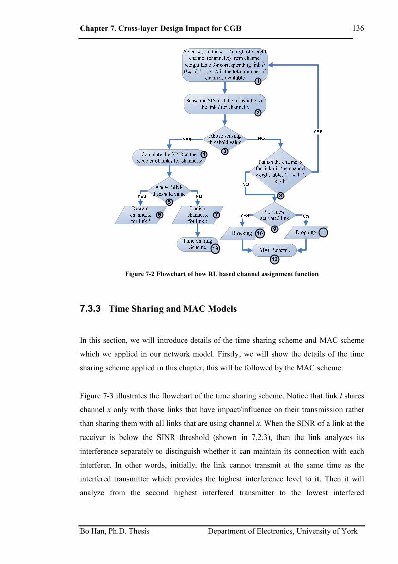
Chapter 7. Cross-layer Design Impact for CGB
Bo Han, Ph.D. Thesis Department of Electronics, University of York
136
Figure 7-2 Flowchart of how RL based channel assignment function
7.3.3 Time Sharing and MAC Models
In this section, we will introduce details of the time sharing scheme and MAC scheme
which we applied in our network model. Firstly, we will show the details of the time
sharing scheme applied in this chapter, this will be followed by the MAC scheme.
Figure 7-3 illustrates the flowchart of the time sharing scheme. Notice that link l shares
channel x only with those links that have impact/influence on their transmission rather
than sharing them with all links that are using channel x. When the SINR of a link at the
receiver is below the SINR threshold (shown in 7.2.3), then the link analyzes its
interference separately to distinguish whether it can maintain its connection with each
interferer. In other words, initially, the link cannot transmit at the same time as the
interfered transmitter which provides the highest interference level to it. Then it will
analyze from the second highest interfered transmitter to the lowest interfered

Chapter 7. Cross-layer Design Impact for CGB
Bo Han, Ph.D. Thesis Department of Electronics, University of York
137
transmitter. Iif the SINR of the link is still below the SINR threshold, then link l also
cannot transmit at the same time as the second highest interfered transmitter. The
modified interference level will keep being re-evaluated until the SINR of the link is
below the SINR threshold (stage 3 to 6 in Figure 7-3), so that the current ith highest
interfered transmitter and the rest of transmitters can transmit simultaneously with link l
by using the same channel.
Figure 7-3 Flowchart of time sharing scheme
The following are the assumptions made to prevent packet collisions.
• Receiver nodes can distinguish the number of interfered transmitters as well as
their individual interference level, so that each link has an interference list to
indicate from highest interfered transmitter to the lowest one.
• We assume the time sharing scheme is symmetrical, which means if link A
detects that it cannot transmit simultaneously with links B and C, then links B
and C are also aware that they cannot transmit at the same time as link A
regardless whether their SINR value at the receiver is above the SINR threshold.

Chapter 7. Cross-layer Design Impact for CGB
Bo Han, Ph.D. Thesis Department of Electronics, University of York
138
• A perfect sharing scheme is applied here to make sure that each link occupies a
different time slot with its interfered links.
Time division multiple access is used here to allow different links to access the full
channel bandwidth at different times. A time unit (T) is subdivided into M notional time
slots where T indicates the time taken at the current event. So the link can transmit at a
high data rate within its assigned time slots. For example, in Figure 7-4, links A, B, C
and D all use the same channel to fulfil their own transmissions. After the time sharing
process in Figure 7-3, it appears that link A cannot transmit at the same time as links B
and C, but can transmit at the same time as link D, thus we say that link A needs to be
time shared with B and C. Therefore, only M/3 time slots can be assigned to link A
during time T. The higher number of links that are time shared with a link, the fewer
time slots can be assigned to the link. More details of the time sharing scheme of Figure
7-4 can be found in Table 7-6, link A and C can be only assigned with M/3 time slots
each to fulfil its transmission on this channel; only M/4 time slots can be allocated for
each link B and C. Although the detail of how and when time slots are assigned to each
transmission is beyond the scope of this thesis, one of example is illustrated in Figure
7-5 to help the reader to understand the concept of the time sharing scheme we applied.
Notice that our time sharing scheme is not the most efficient scheme as there is 1/6
channel wasted due to the M/6 time slots that are not assigned to any link as shown in
Figure 7-5.
Figure 7-4 Example of links sharing different time
Links A B C D
A N/A N N Y
B N N/A N N
C N N N/A N
D Y N N N/A
Table 7-6 Table of the time sharing scheme; N/A indicates not available; N represents links cannot
transmit at the same time; Y means links can transmit at the same time.

Chapter 7. Cross-layer Design Impact for CGB
Bo Han, Ph.D. Thesis Department of Electronics, University of York
139
Figure 7-5 Example of how time slots are assigned to each link
Packet collisions will not take place in this scenario due to the application of the perfect
time sharing scheme. In practice, real MAC schemes will generate overheads to achieve
such behaviour. Therefore, retransmission only takes places where the transmitter
detects that no channels can be available for its transmission due to the interference
level it suffers. Hence, the transmitter of the link senses the status on all the channels
until one of them becomes idle. Then, the link will start its transmission. Figure 7-6
illustrates the flowchart of the proposed MAC scheme we use. The proposed MAC
scheme is similar to the 1-persistant CSMA scheme.
Figure 7-6 The flowchart of the MAC scheme

Chapter 7. Cross-layer Design Impact for CGB
Bo Han, Ph.D. Thesis Department of Electronics, University of York
140
7.4 Cognitive Cross-layer Design
The channel assignment and routing should be jointly considered as both schemes will
be invoked when there is a change in the network topology [84]. In this section, we will
introduce the benefit of associating cognitive greedy-backhaul routing (CGB) with a
reinforcement learning based channel assignment scheme (RLCAS) by comparing with
other combinations of varying routing with varying channel assignment schemes such
as shortest path by hops (SH) with RLCAS, shortest path by hops (SH) with sensing
based channel assignment scheme (SCAS) and interference level based routing (ILR)
with RLCAS.
7.4.1 CGB with RLCAS
Since the details of CGB routing have been introduced in the last chapter, we know that
CGB prefers to select links that are heavily utilized, which means CGB invokes fewer
nodes to relay network traffic. Thus, energy consumption can be minimized by
switching nodes into sleep mode except for active nodes. The reinforcement learning
based channel assignment scheme (RLCAS) with CGB (CGBRL) can form an efficient
cross-layer design due to the route selection feature of CGB, which provides a relatively
slowly changing environment for RLCAS as it prefers links that have been currently
utilized to new ones. With a suitable channel assignment scheme, channels can be
allocated efficiently around the network without or with limited interference, so that
additional capacity is assigned to crowded links where needed. In addition, the link
weight of CGB depends on the channel utilization level which requires cross-layer
information from the channel assignment protocol. Therefore, the cross-layer design of
combining CGB with RLCAS not only can reduce the complexity for the channel
assignment scheme but also improve the capacity of wireless ad hoc networks as well as
reducing network energy consumption.

Chapter 7. Cross-layer Design Impact for CGB
Bo Han, Ph.D. Thesis Department of Electronics, University of York
141
7.4.2 SH with RLCAS and SCAS
SH can also associate well with RLCAS (SHRL) as it selects a fixed path from a specific
source to a specific destination as long as the network topology remains the same. This
feature of route selection provides a relatively stable environment for RLCAS.
Although SHRL can deliver similar performance on channel selection as CGBRL, it does
not take other network factors into consideration when establishing paths. Therefore
CGBRL can outperform SHRL in network energy consumption as it prefers to relay
traffic through those nodes that have already been activated.
Associating SH with SCAS (SHSensing) can show how the channel assignment scheme
impacts on the network performance when the same routing is applied. The following
section will show the result that a better channel assignment scheme can have a more
significant impact on overall network performance than a better routing strategy.
7.4.3 ILR with RLCAS
In low traffic demand wireless networks where the radio spectrum is sufficient to fulfil
traffic flows, it is encouraged to route around current existing traffic flows without
potentially reducing the network capacity. Traditional ad hoc routing metrics, like
shortest path, cannot take the interference level into account. Higher capacity links
might remain unused and lower capacity links might end up being crowded. As a result,
in wireless ad hoc networks, it is essential to relay more traffic through the higher
capacity links so that network capacity can be improved.
In chapter 3, we presented a family of interference routing metrics whose link weight is
calculated based on the number of disturbed nodes within the interference range which
is defined as a fixed circle around the transmitting node. Here, the interference level is
calculated in a more practical way as the ILR routing algorithm is based on the
summation of the interference level that a node suffers on each channel. The received
interference level from unexpected transmitters is determined by the path loss model

Chapter 7. Cross-layer Design Impact for CGB
Bo Han, Ph.D. Thesis Department of Electronics, University of York
142
and the transmit power which are illustrated in the previous sections. The link weight of
ILR is determined by:
{ }||321
||
1
......,,;,, Pc
P
Xcij IIIIIVjiIw ∈∈∀∑=
=
(7.8)
Where Ic is the received power of node j by all transmitters using channel c. |P| is the
total number of channels in the network.
One of the disadvantages of ILR routing is the relaying burden it generates. ILR tries to
route around congested nodes/links as they suffer significant interference. Therefore,
there may not be sufficient channels in the network due to the extra relaying ILR
generates. Another disadvantage of ILR routing is the dynamic feature of route
establishment as the link weight depends on the current interference level which is
related to the traffic pattern. This results in a difficult learning environment for RLCAS
as the environment changes faster than the process of learning.
7.5 Capacity Analysis
In this section, we will use mathematical analysis to illustrate the upper bound and
lower bound capacity a link can obtain in our network model.
L denotes the expected path length that a packet is traversed from a source node to a
destination node. Then, the minimum hop number of the path is
r
LH =
(7.9)
where r is the transmission range of each node. Therefore, the minimum number of
activated links at certain traffic load λ is

Chapter 7. Cross-layer Design Impact for CGB
Bo Han, Ph.D. Thesis Department of Electronics, University of York
143
λr
LLN =
(7.10)
As the traffic load in this thesis represents the number of path flows, W represents a
channel’s maximum capacity. In the worst case scenario all of these links are assigned
to an identical channel and are close to each other so that they have to share the capacity
due to their interference. The capacity of each link can only obtain a portion of the
channel capacity with respect to the number of activated links.
Considering the shortest path by hops routing metric (SH) here, then the expected
number of links is λr
Las it can generate the minimum hop number amongst all routing
metrics. This is the lower bound capacity for a link (using SH).
N
LL
WC =
(7.11)
In the best case scenario where all links are far away from each other, channel capacity
can be utilized by each of them due to channel spatial reuse. Then the capacity of each
link can obtain the maximum channel capacity. This represents the upper bound
capacity for a link.
WCU = (7.12)
We can define the capacity of a link as
N
N
l LL
WC ≤≤= δδ 1,
(7.13)
where δ represents the parameter of channel spatial reuse which is affected by node’s
transmission range, path loss model, channel assignment scheme, SINR threshold etc. It
is between 1 (lower bound) and LN (Lλ/r - upper bound). If δ approaches the expected
number of activated links, the scheme is considered to be better as a lower number of

Chapter 7. Cross-layer Design Impact for CGB
Bo Han, Ph.D. Thesis Department of Electronics, University of York
144
links share a channel temporally due to more efficient channel spatial reuse. In this case,
links which have been assigned with the same channel are far away so that the
transmissions can be carried simultaneously. In contrast, if δ approaches to 1, the
number of links which are sharing the same channel increases. To avoid channel
collisions, those links have to share the channel temporally so that results in lower
obtainable capacity for each of them due to the high competition.
Since the parameters of r, λ, W are fixed and known in our network model, in order to
determine a link’s capacity we have to find out the expected path length which is
influenced by the routing metric design. It is quite difficult to deduce the path length of
certain routing metric designs as the path length is not only related to the network area
but is also related to the weight function we defined for the routing metric. Therefore,
we will only provide the expected path length of using shortest path by hops (minimum
hop count) as the path length is only a function of network area instead of routing
metric due to its fixed weight function.
In [30], Li shows the probability density function (pdf) giving the probability of a node
communicating with another node at distance x as
A
x
dtt
xp
Ax
2
0
==
∫
(7.14)
where A indicates the network area and the integral is from 0 to A as A is the
maximum distance a path can traverse using shortest path by hops for a square network
when the source node or the destination node is selected at the centre of the network.
Therefore, the expected path length for a random traffic pattern is
3
2)(
0
AdxxxpL
A
== ∫
(7.15)

Chapter 7. Cross-layer Design Impact for CGB
Bo Han, Ph.D. Thesis Department of Electronics, University of York
145
This expected path length is only valid for the shortest path routing metric. Other
routing metrics should have larger path length as they generate more relaying hops and
traverse longer distances. The shortest path by hops has the lowest expected path length
among all routing metric designs, which proves that routing metric design should take
path length into account in order to improve channel capacity. From equations (7.10),
(7.13) and (7.15), we can deduce the link capacity of the shortest path by hops routing
metric if we can determine maximum channel capacity, transmission range, traffic load,
channel spatial reuse factor (δ) and network size:
NSl LA
rWC ≤≤= δδ
λ1,
2
3,
(7.16)
7.6 Energy Performance
In this section, we compare the network performance by using the proposed cross-layer
design, cognitive-greedy backhaul routing with reinforcement learning based channel
assignment scheme (CGBRL), the shortest path by hops (SH) with sensing based channel
assignment scheme (SHSensing), the shortest path by hops with RL based channel
assignment scheme (SHRL) and the interference level routing with reinforcement
learning based channel assignment scheme (ILRRL).
Figure 7-7 shows the average network energy consumption in a best case scenario (a)
and a worst case scenario (b) using different schemes. Both scenarios illustrate that
CGBRL has significantly reduced energy consumption compared with the others. Each
point along each result is collected based on the total network energy cost from the first
event to the last event among 5 repeated simulations at a certain network traffic load.
Initially, CGB relays traffic from source to destination based on minimum hop count as
SH and then forces other traffic to a flow through the popular links due to their
important geographical locations to build trunked backhaul links. Therefore CGB uses
the minimum number of activated nodes (transmitting or receiving) to fulfil its
transmission. Comparing CGBRL with SHRL and ILRRL, the results of delay are similar
as they are using the same channel assignment scheme, whereas CGB improves the

Chapter 7. Cross-layer Design Impact for CGB
Bo Han, Ph.D. Thesis Department of Electronics, University of York
146
energy consumption up to 35% and 51% respectively in the best case scenario, due to
the unnecessary relaying/nodes that is generated/invoked by SH and ILR. Although
traffic flows are concentrated in the backhaul links, the RL based channel assignment
scheme can provide additional capacity by allocating channels efficiently without
causing hidden terminal problems, so that activated links can have the maximum
channel capacity for transmission as time sharing contention occurs less frequently. As
aforementioned in the energy consumption model section, the total network energy
consumption (Etotal) is also a time constraint as it relates not only to the number of nodes
in different power modes but also to each event time. Hence, a poor channel assignment
scheme results in a longer delay, which indicates a longer activation time for activation
nodes. For example, the sensing based channel assignment scheme (SPSensing) cannot
solve the hidden terminal problem; thereby delay is increased due to the inefficient
channel allocation methodology as shown in Figure 7-8. SHRL improves the total
network energy consumption up to about 31% and 23% compared with SPSensing in the
best and worst case scenarios respectively, even when the same routing strategy is
applied. In addition, CGBRL illustrates a greater advantage on energy saving by
increasing the network traffic load. This is due to CGB which relays traffic through
nodes that have already been activated, whereas SH requires many more nodes to relay
its traffic thereby increasing the overall network traffic load.
(a)

Chapter 7. Cross-layer Design Impact for CGB
Bo Han, Ph.D. Thesis Department of Electronics, University of York
147
(b)
Figure 7-7 Average network energy consumption with different schemes against network traffic
load in the (a) best case scenario, (b) worst case scenario
7.7 Delay and Throughput Performance
Figure 7-8 shows the average delay against network traffic load among different
schemes. Each point along each result is collected based on the mean delay among all
activated end-to-end traffic flows from the beginning of the events to the last event for a
certain network traffic load. Intuitively, SHRL should outperform in terms of delay
compared with the other schemes as SH routing generates the lowest relaying burden in
the network. Nevertheless, CGBRL and ILRRL have similar performance to the SHRL.
This is because they all use the same channel assignment scheme, reinforcement
learning based channel assignment scheme (RLCAS). With a relatively slowly changing
environment, e.g. end-to-end traffic flows remaining in the network for sufficient
events, the learning engine of RLCAS can obtain enough environment information in
order to assign channels in a more efficient way. Despite the routing schemes we
applied, a good RL based channel assignment scheme in a slow changing network
environment, it should aim to allocate suitable channels for links with regard to their
locations. In other words, channel assignment should adapt well with environment
changes such as traffic pattern, nodes movement etc. As shown in Figure 7-8, CGBRL,

Chapter 7. Cross-layer Design Impact for CGB
Bo Han, Ph.D. Thesis Department of Electronics, University of York
148
SPRL and ILRRL reduce the average traffic delay significantly, compared with SPSensing
by up to about 47%, 37% and 31% respectively. The sensing based channel assignment
scheme cannot detect hidden terminals, and therefore channel interference occurs and
channel capacity is shared by those links time sharing with each other as shown in
Figure 7-3. Finally, delay is increased as less channel capacity is allocated for those
transmissions due to the contention on the same channel.
Figure 7-8 Average delays with different schemes against network traffic load
Figure 7-9 further proves the result shown in Figure 7-8 as the time sharing probability
of using a sensing based channel assignment scheme is much greater than the
reinforcement learning based channel assignment scheme with different routings. The
time sharing probability indicates how often the time sharing scheme occurs using each
scheme. Since the sensing based channel assignment scheme cannot detect the
interference level at the receiver end of the link, it suffers from the hidden terminal
problem when assigning channels. Although the reinforcement learning-based channel
assignment scheme is not a perfect solution for solving the hidden terminal problem,
with the learning knowledge it gains from the environment which includes the traffic
pattern, neighbour channel utilization etc., it is able to punish the bad channels and
reward the good ones. Therefore the future decision on the channel selection will be
influenced by the learning knowledge gained from past, so RLCAS is a better solution
for solving hidden terminal problem than SCAS.
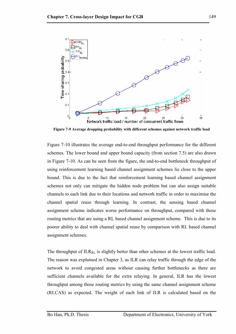
Chapter 7. Cross-layer Design Impact for CGB
Bo Han, Ph.D. Thesis Department of Electronics, University of York
149
Figure 7-9 Average dropping probability with different schemes against network traffic load
Figure 7-10 illustrates the average end-to-end throughput performance for the different
schemes. The lower bound and upper bound capacity (from section 7.5) are also drawn
in Figure 7-10. As can be seen from the figure, the end-to-end bottleneck throughput of
using reinforcement learning based channel assignment schemes lie close to the upper
bound. This is due to the fact that reinforcement learning based channel assignment
schemes not only can mitigate the hidden node problem but can also assign suitable
channels to each link due to their locations and network traffic in order to maximise the
channel spatial reuse through learning. In contrast, the sensing based channel
assignment scheme indicates worse performance on throughput, compared with those
routing metrics that are using a RL based channel assignment scheme. This is due to its
poorer ability to deal with channel spatial reuse by comparison with RL based channel
assignment schemes.
The throughput of ILRRL is slightly better than other schemes at the lowest traffic load.
The reason was explained in Chapter 3, as ILR can relay traffic through the edge of the
network to avoid congested areas without causing further bottlenecks as there are
sufficient channels available for the extra relaying. In general, ILR has the lowest
throughput among those routing metrics by using the same channel assignment scheme
(RLCAS) as expected. The weight of each link of ILR is calculated based on the

Chapter 7. Cross-layer Design Impact for CGB
Bo Han, Ph.D. Thesis Department of Electronics, University of York
150
summation of power received from all activating transmitters. Due to the characteristic
of ILR, extra hops are needed which consumes more network capacity. In addition, ILR
encourages the upcoming traffic flow to shift to a less crowded area due to the
concurrent interference levels. This dynamic routing selection results in an inefficient
learning process for RLCAS as the link usage of using ILR is much smaller than CGB
(evidence can be found in next section). Intuitively, ILRk and ILRth (illustrated in
Chapter 4) consume more network capacity compared with ILR under high traffic load
conditions.
An interesting point is that using different channel assignment schemes can improve the
network performance more significantly than using different routing strategies. As
shown in Figure 7-10, SH only improves the network average throughput up to about
14% by comparison with ILR when RLCAS is applied to both routing schemes,
whereas RLCAS shows a throughput improvement of up to 61% by comparison with
SCAS when the same SH routing is used. As expected from (7.13), in Figure 7-10,
RLCAS illustrates a better channel spatial reuse (better δ) than SCAS by using the
shortest path by hops routing metric design. In a poor channel assignment scheme, more
links compete for the same channel which results in lower obtainable capacity for each
link. Comparing the two schemes RLCAS with ILR and RLCAS with SH, RLCAS with
SH shows much better results in end-to-end throughput as the expected path length of
using ILR is much longer than using SH. This implies that a good routing metric design
should take path length into account in order to reduce relaying burden impact. In
equation (7.13), although shortest path by hops has the lowest path length and both
schemes of CGB with RLCAS and SH with RLCAS use a reinforcement learning based
channel assignment scheme, CGB with RLCAS provides a better end-to-end throughput
in Figure 7-10. This is due to a better channel spatial reuse (better δ) as reinforcement
learning based channel assignment scheme can combine better with a CGB routing
metric than shortest path by hops routing metric (more details are given in Figure
7-11and Figure 7-12).

Chapter 7. Cross-layer Design Impact for CGB
Bo Han, Ph.D. Thesis Department of Electronics, University of York
151
Figure 7-10 Average end-to-end throughput with different schemes against network traffic load
7.8 Learning Performance
The learning process of channel assignment can not only adapt with environment
changes but can also affect the environment. Each decision of channel selection on a
link affects the channel learning process of the other links. For instance, a bad learning
process can reduce channel capacities due to co-channel interference and results in a
longer occupation time on those channels; consequently, they will affect channel
selections and learning process for other upcoming links. On the other hand, if a good
channel decision is made, the traffic flow can fulfil the transmission task in a more
efficient way and results in a shorter lifetime. Thus, more channels can be available for
upcoming transmissions. A better reward can be achieved during a longer process if
learning adapts well with the environment.
Figure 7-11 shows the Cumulative Distribution Function (CDF) performance on the
utilization of links (link usage) by applying different routing metrics at an average
traffic load of 31.5 end-to-end traffic flows. The x-axis (link usage) is plotted on a
logarithmic scale. The utilization level of a link (link usage) is the number of times that
the link has been activated. In CGB link usage, about 8% and 5% of total links exceed
the maximum link usage of ILR (max utilization level = 43) and SH (max utilization

Chapter 7. Cross-layer Design Impact for CGB
Bo Han, Ph.D. Thesis Department of Electronics, University of York
152
level = 70) respectively and the maximum link usage among CGB links is about 248
which is around 6 times and 4 times than the maximum link usage of ILR and SH
respectively. As expected, CGB has the ability to attract traffic flows through certain
backhaul links due to their geographical location and SH has regular link usage levels
among links due to the stable topology and the lack of ability to find alternative links
for traffic relaying. ILR obtains on average low levels of link utilization as it disperses
its transmission tasks to less interfered links. Those high utilization levels of links
reflect the exploration ability to detect good channels as well as bad channels around
them. In other words, the learning progress of each link is proportional to its link usage
which is related to the routing metric we applied and the traffic pattern.
Figure 7-11 CDF of link usage at a traffic load of 31.5 traffic flows
A higher link usage indicates a better opportunity for a link to explore and exploit its
most suitable channels as well as bad channels that are occupied in the vicinity with
respect to the environment. CGB has more opportunities for links to find suitable
channels as there are 5% and 9% of total links that have channel weight values which
exceed 72 (highest weight value by using SH) and 40 (highest weight value by using
ILR) by comparison with SH and ILR respectively. This result can be seen in Figure
7-12 which is the CDF of channel weight value at the same traffic load as in Figure 7-11.
The graph only shows the extreme conditions of high and low weight values as the
middle range of channel weight values has similar performance among these routing
metrics. In the high weight value section (graph a), a certain channel weight is rewarded
with as high as 1090, 963 and 951 for CGB, SH, and ILR links respectively. This is due

Chapter 7. Cross-layer Design Impact for CGB
Bo Han, Ph.D. Thesis Department of Electronics, University of York
153
to the higher usage of those links that gain more opportunity to use and reward its best
channels than those links with a low utilization level. On the other hand, in the low
weight value section (graph b), although a few channel weights of CGB received
punishment as low as -330 compared to the minimum channel weight value of SH (-42)
and ILR (-29), CGB still outperforms the other routing metrics in terms of time sharing
probability, delay and throughput performance as shown in Figure 7-8, Figure 7-9 and
Figure 7-10. The reasons are as follows. There are excessive activated links that require
bandwidth for their transmissions as the performance is measured under an extremely
high traffic load condition (31.5 concurrent traffic flows), as well as the routing
behaviour of CGB which accumulates those transmissions through backhaul links.
Therefore, some bad channels are punished due to the excessive interference in the
vicinity that is detected by the sensing scheme so that the link will avoid using those
bad channels in future events. In other words, the large punishment value of links on
certain channels does not indicate an inefficient learning progress; in contrast, it
explores those channels that are preferred by its neighbour links in order to avoid
channel collisions when it selects its own channels for transmissions. Conclusively, the
learning progress of a link on channel assignment is proportional to the link’s utilization
level as a higher utilization level indicates more opportunities for the link to find the
good channels and bad channels in its local environment.
Figure 7-12 CDF of channel weight value at a traffic load of 31.5 traffic flows; graph (a) shows the
extreme weight values at large reward section; graph (b) shows the extreme weight values at large
punishment section

Chapter 7. Cross-layer Design Impact for CGB
Bo Han, Ph.D. Thesis Department of Electronics, University of York
154
7.9 Conclusion
This chapter has shown the impact of cross-layer design in a more practical network
environment by including a path loss model, a better interference model and traffic
models as well as an energy model. It also studied each cross-layer scheme by
associating different combinations of routing with each channel assignment scheme. A
novel cross-layer design that combines the cognitive greedy-backhaul routing with the
reinforcement learning based channel assignment scheme shows that RLCAS can be
incorporated reasonably into CGB by assigning extra capacity to the backhaul links, and
CGB uses a limited number of nodes to relay traffic flows. Our results show that the
proposed cross-layer design of CGB with a RL based channel assignment scheme
reduces the energy consumption without compromising throughput and delay. In
addition, the learning progress of links on channel selections is examined with respect
to the link usage. The results show that the CGB has the best ability to explore the good
channels as well as the bad channels due to the routing behaviour of attracting
transmissions through backhaul links which result in high link utilization levels.

Chapter 8. Exploiting RL Channel Assignment Scheme
Bo Han, Ph.D. Thesis Department of Electronics, University of York
155
Chapter 8
8 Exploiting a RL Channel Assignment
Scheme
Contents _____________________________________________________________________
8 Exploiting a RL Channel Assignment Scheme .....................................................155
8.1 Introduction ...................................................................................................155
8.2 Network Scenario..........................................................................................157
8.3 RL Channel Assignment Scheme without Sensing.......................................158
8.4 Performance ..................................................................................................159
8.4.1 Network Performance ...........................................................................159
8.4.2 Learning Performance Based on Traffic Loads ....................................163
8.4.3 Learning Performance Based on Distance (hop)...................................165
8.4.4 Learning Performance Based on Link Usage........................................168
8.5 Conclusion.....................................................................................................169
_____________________________________________________________________
8.1 Introduction
From the previous chapter, we have seen that the cross-layer design of combining the
reinforcement learning based channel assignment scheme (RLCAS) with cognitive
greedy-backhaul (CGB) routing is a key technique to reduce network energy
consumption while still maintaining other network performance in terms of end-to-end
bottleneck throughout and delay. We also proved that applying a better channel
assignment scheme can show a greater advantage than applying a better routing scheme.
Therefore, in this chapter, we will further study the impact of applying different channel
assignment schemes with CGB routing. Moreover, we will analyse the learning progress

Chapter 8. Exploiting RL Channel Assignment Scheme
Bo Han, Ph.D. Thesis Department of Electronics, University of York
156
of RLCAS, and elaborate how the channel assignment benefits from the learning
engine.
Maintaining network capacity is a big challenge for wireless ad hoc networks due to
their multi-hop feature. Although relaying can help convey data on a multi-hop basis,
the relayed traffic also need channel capacity. In wireless networks, the available
frequency spectrum is precious and limited, and therefore channel spatial reuse is vital
to increase network capacity. Hence, a proper channel assignment scheme is required
for wireless ad hoc networks to allocate channels in a distributed manner for the large
number of relaying links in order to reduce the blocking and dropping probability, as
well as maximizing network QoS [85]. Traditional cellular channel assignment schemes
are not suitable for wireless ad hoc networks. Fixed channel assignment (FCA) cannot
be applied to wireless ad hoc networks as there is no central base station to allocate
fixed channels to certain locations. In addition, FCA cannot adapt with environment
changes such as changing of traffic conditions and user movement. Although dynamic
channel assignment (DCA) can solve the problems from which FCA suffers, it has been
proven that DCA does not perform well under heavy traffic load conditions [86]. In
[84], Gong introduces a cross-layer design by combining the OLSR routing protocol
with a channel assignment scheme to reduce channel collisions in wireless ad hoc
networks. Gong’s idea is to use the routing control messages of OLSR to exchange
channel information up to k-hops. Therefore, it requires a significant control overhead
up to k-hops to be able to reduce channel collisions caused by the hidden node problem.
Due to the decentralized nature of wireless ad hoc networks, we need a channel
assignment scheme where transmitters can decide which channels are suitable for use in
an autonomous process. Some research has proposed that users/nodes could find
suitable channels in a distributed way by applying machine learning into the channel
assignment scheme [76, 80, 87]. Although there are some research works using machine
learning based channel assignment schemes, most of them focus on a single hop basis
instead of a multi-hop basis. Therefore, the purpose of this chapter is to examine the
learning process of using reinforcement learning based channel assignment schemes in a
multi-hop approach associated with routing metric design.

Chapter 8. Exploiting RL Channel Assignment Scheme
Bo Han, Ph.D. Thesis Department of Electronics, University of York
157
The contents of this chapter are structured as follows. Firstly, we illustrate the network
scenario. Next, we discuss the varying channel assignment scheme with CGB routing.
This is followed by performance comparison results. We compare the results especially
on the learning process of reinforcement learning based channel assignment schemes
with and without sensing. Finally, conclusions will be given.
8.2 Network Scenario
The network parameters such as network size, node number, number of available
channels, traffic model and path loss model have been provided in the previous chapter.
Figure 8-1 shows the network layout. There are 100 nodes in total; top number indicates
the node index; bottom number indicates the number of hops away from the destination
node (node index 100 – indicated by a black triangle).
Figure 8-1 Network layout

Chapter 8. Exploiting RL Channel Assignment Scheme
Bo Han, Ph.D. Thesis Department of Electronics, University of York
158
8.3 RL Channel Assignment Scheme without Sensing
From Chapter 7, we have seen that a reinforcement learning based channel assignment
scheme (plus sensing) when combined with a shortest path (SH) routing algorithm can
deliver superior network performance, compared with a sensing based channel
assignment scheme (SCAS) with SH. With the reinforcement learning based channel
assignment scheme plus sensing, nodes can be aware of their neighbours’ environment,
and therefore eliminate the probability of channel collision in their vicinity. Although
channel collisions can be limited by the sensing ability of each transmitter, channel
collisions may still occur at the receivers due to the hidden node problem that was
mentioned in Chapter 7. However, the sensing technique cannot solve the hidden node
problem; it increases the control overhead and energy consumption, and it introduces
the exposed node problem [88]. The exposed node problem occurs when a node is
prevented from initiating packet transmission to other nodes due to the adjacent
transmitter(s). Consider an example of 4 nodes (A, B, C and D) as shown in Figure 8-2
where two receivers A and D are out range of each other, but the two transmitters B and
C are in range of each other. Theoretically, transmissions could happen simultaneously
by using same channel as the destinations (A and D) are out of range of each other. In
contrast, as node B starts to send its signal to A, node C is prevented from transmitting
to D as it wrongly thinks a collision will happen due to carrier sense. This problem
could limit the efficiency of channel spatial reuse. Therefore, we test the reinforcement
learning without a sensing based channel assignment scheme (RL-NS-CAS) to study the
learning impact on the channel assignment without sensing. Figure 8-3 illustrates the
flowchart of RL-NS-CAS. Compared with the reinforcement learning based channel
assignment scheme with sensing (RLCAS), RL-NS-CAS selects the highest weight
channel and uses it straight away without sensing the channel status.
Figure 8-2 Exposed node problem
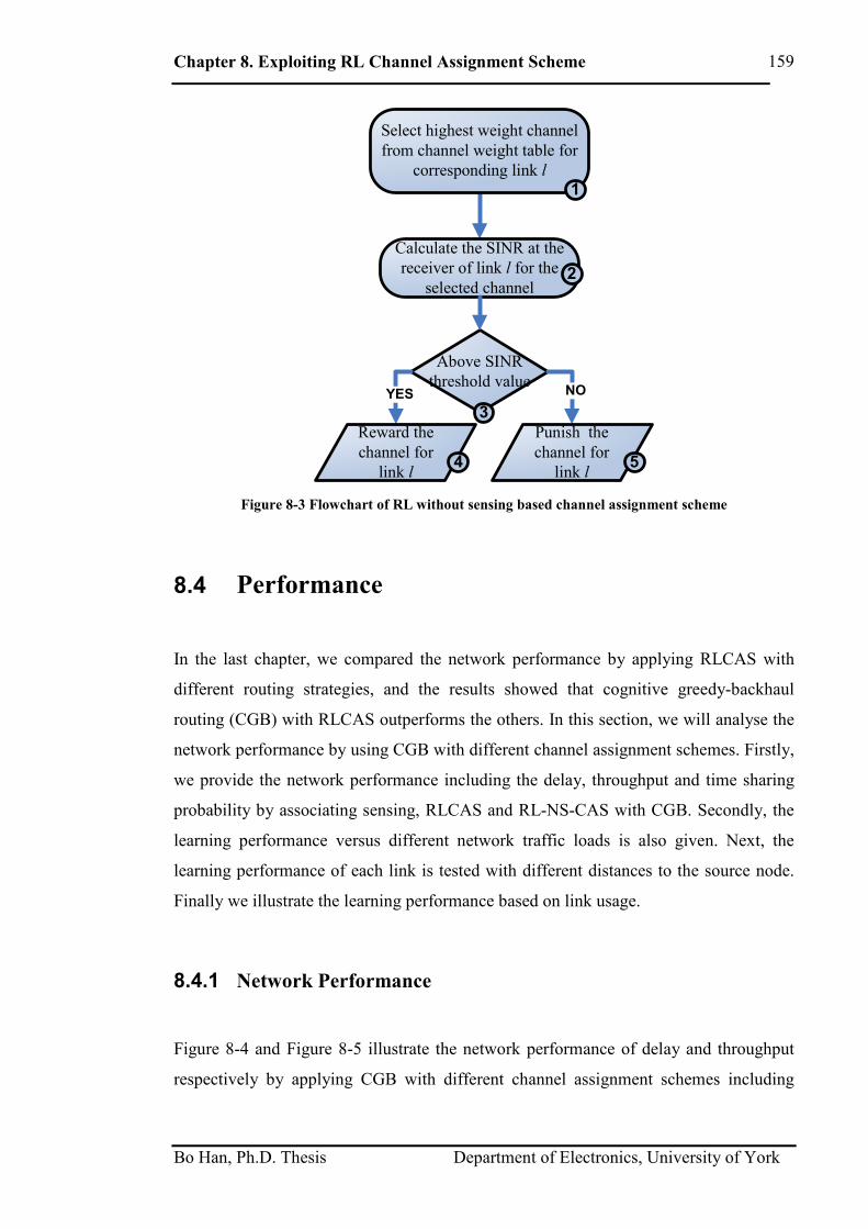
Chapter 8. Exploiting RL Channel Assignment Scheme
Bo Han, Ph.D. Thesis Department of Electronics, University of York
159
Select highest weight channel
from channel weight table for
corresponding link l
Calculate the SINR at the
receiver of link l for the
selected channel
Above SINR
threshold valueYES
Reward the
channel for
link l
NO
Punish the
channel for
link l
1
2
3
4 5
Figure 8-3 Flowchart of RL without sensing based channel assignment scheme
8.4 Performance
In the last chapter, we compared the network performance by applying RLCAS with
different routing strategies, and the results showed that cognitive greedy-backhaul
routing (CGB) with RLCAS outperforms the others. In this section, we will analyse the
network performance by using CGB with different channel assignment schemes. Firstly,
we provide the network performance including the delay, throughput and time sharing
probability by associating sensing, RLCAS and RL-NS-CAS with CGB. Secondly, the
learning performance versus different network traffic loads is also given. Next, the
learning performance of each link is tested with different distances to the source node.
Finally we illustrate the learning performance based on link usage.
8.4.1 Network Performance
Figure 8-4 and Figure 8-5 illustrate the network performance of delay and throughput
respectively by applying CGB with different channel assignment schemes including

Chapter 8. Exploiting RL Channel Assignment Scheme
Bo Han, Ph.D. Thesis Department of Electronics, University of York
160
sensing based, reinforcement learning with sensing and without sensing based schemes.
The CDF results are analysed from a large amount of data which was collected through
Monte-Carlo simulations using between 1 and 40 traffic flows at various traffic loads.
Both results show a great advantage by using a learning-based channel assignment
scheme with CGB, compared with the sensing based channel assignment scheme with
CGB. As can be seen in Figure 8-4, with RLCAS and RL-NS-CAS the delay is
improved by up to about 26% and 16% respectively compared with SCAS (at delay
value of 43 seconds). Moreover, throughput using SCAS is only above 8.6 Mbps 9% of
the time, compared with 52% and 58% when using RL-NS-CAS and RLCAS as shown
in Figure 8-5. As a result, the learning based channel assignment schemes deliver a
better network QoS in delay and throughput than a purely sensing-based channel
assignment scheme, as links are able to find their preferred channels through learning
about their environment, in order to avoid hidden node problems.
Figure 8-4 CDF of long-term end-to-end delay by using CGB with different channel assignment
schemes

Chapter 8. Exploiting RL Channel Assignment Scheme
Bo Han, Ph.D. Thesis Department of Electronics, University of York
161
Figure 8-5 CDF of long-term end-to-end throughput by using CGB with different channel
assignment schemes
Figure 8-6 shows the time sharing probability against network traffic load graph, using
the time sharing scheme that was proposed in Chapter 7, where links are allocated to
different time slots if they cannot use the same channel concurrently. This figure
explains that the SCAS cannot avoid the occurrence of channel collisions and the
probability of time sharing increases as network traffic load rises. Nevertheless, learning
based channel assignment schemes have the ability to reduce the hidden node problem
as they show a dramatic reduction of time sharing probabilities compared with SCAS.
Figure 8-6 shows that using RL-NS-CAS and RLCAS, there are about 33% and 35%
reductions on the time sharing probability than SCAS at a traffic load of 35 traffic
flows. Furthermore, the graph illustrates learning based channel assignment schemes
can maintain the time sharing probability at a similar level which is about 1% to 5%,
even with the increasing of the network traffic load from 2 to 28 traffic flows.
Therefore, this result indicates that for the network environment (includes network size,
node number, transmission range, SINR threshold and etc.) used for this chapter, 100
channels are sufficient under a traffic load of 28 concurrent traffic flows and channel
spatial reuse can be obtained through learning. On the other hand, the channel capacity
reduces significantly when traffic load is above 28 flows as there is no additional
channel capacity to fulfil those transmissions and relaying, and time sharing probability
starts rising quickly with the increasing of the network traffic load. It is also to
mentioning that RLCAS demonstrates a significant advantage on time sharing

Chapter 8. Exploiting RL Channel Assignment Scheme
Bo Han, Ph.D. Thesis Department of Electronics, University of York
162
probability over RL-NS-CAS at very high traffic load. This is due to the different
exploration abilities: RLCAS can adapt and react more efficiently with its sensing
ability in a high traffic load network, whereas RL-NS-CAS adapts relatively slowly in a
fast changing environment.
Figure 8-6 Average time sharing probability by using CGB with different channel assignment
schemes against network traffic load
The aim of using a reinforcement learning based channel assignment scheme is to
assign channels through a distributed approach where links/nodes can find their
preferred channel/channels even with environment changes such as node movements
and traffic patterns. The sensing can improve the efficiency of the exploration stage
when the environment changes. Links can reward the good channels or punish the bad
channels through learning in a relatively static environment to maximize the
exploitation stage of reinforcement learning. In other words, the exploration stage of
reinforcement learning-based channel assignment schemes function as DCA at the
initial stage, so that suitable channels can be assigned to each activated link due to their
positions and traffic patterns in order to avoid channel collisions. With the assistance of
sensing, reinforcement learning can explore the environment more efficiently. After a
long time operating the learning process, RLCAS performs more like FCA as links are
allocated with fixed channel/channels with respect to their different locations in order to
improve the channel spatial reuse.

Chapter 8. Exploiting RL Channel Assignment Scheme
Bo Han, Ph.D. Thesis Department of Electronics, University of York
163
8.4.2 Learning Performance Based on Traffic Loads
Figure 8-7 and Figure 8-8 illustrate how learning reacts with different network traffic
loads when applying sensing or without sensing for a reinforcement learning based
channel assignment scheme. The x-axis (the channel weight ranking) is plotted on a
logarithmic scale. Results are collected from a channel weight table which is a |m|-by-
|n| matrix (Cmn) where |m| indicates the total number of links and |n| represents the
number of channels available in the network. In the network scenario shown in Figure
8-1, there are a total of 938 links and 100 channels available in the network. M and N
denote the set of links and the set of channels respectively. To obtain the values of the
y-axis in Figure 8-8 and Figure 8-7, first the matrix Cmn is sorted at each row in a
descending order.
{ }NnnnndescendCsortC nnmnmn ∈≥≥≥= ||||21 ;...),'',( (8.1)
Then we treat the columns of C as vectors, returning a row vector of the sums of each
column. Therefore now we have a vector (W) with 100 elements which indicates the
sums of the channel weight values from the highest rank weight channel to the lowest
rank weight channel among all links.
||,...,2,1,,,1
niCMMmmW mniij
m
j
ji =⊂∈=∑=
(8.2)
Next, we can calculate the total channel weight value by sum of Wi.
ix
n
x
xtotal WWWW ∈= ∑=
,||
1
(8.3)
Finally, the normalized channel weight value of each summation channel weight is
calculated from the highest rank weight channel to the lowest rank weight channel.

Chapter 8. Exploiting RL Channel Assignment Scheme
Bo Han, Ph.D. Thesis Department of Electronics, University of York
164
||,...,2,1; niW
WW
total
inorm ==
(8.4)
These two graphs can illustrate how fast the learning rate is for each scheme under
different network traffic loads. Figure 8-7 shows that the learning rate of the
reinforcement learning based channel assignment scheme with sensing is almost
identical to the scheme without sensing under a low network traffic load condition as
the sum of the high rank weight channels (rank 1 to rank 10 perhaps) accumulate to a
similar weight value through learning. This is due to the environment which changes
relatively slowly under a low traffic load, so that the exploration ability does not have a
significant impact on the learning process although RLCAS shows a better exploration
ability than RL-NS-CAS due to the assistance of sensing. The channel weight values of
the sensing based channel assignment scheme (SCAS) are collected for reference
comparison to those learning schemes. As expected, the channel weight value of SCAS
demonstrates almost a uniform distribution figure as the accumulated channel weights
are based on instantaneous sensing rather than historical learning.
On the other hand, for a high traffic load condition where the network changes
relatively quicker due to the traffic pattern, RLCAS achieves a better learning rate than
RL-NS-CAS at high ranking channel weights between the highest and 10th highest
channel weights. This proves that RLCAS can adapt better and faster to a dynamic
environment than RL-NS-CAS due to its better exploration ability thanks to the sensing.

Chapter 8. Exploiting RL Channel Assignment Scheme
Bo Han, Ph.D. Thesis Department of Electronics, University of York
165
Figure 8-7 Normalized channel weight against channel weight ranking from the highest to the
lowest at a traffic load of 13 traffic flows (low traffic load) with different channel assignment
schemes
Figure 8-8 Normalized channel weight against channel weight ranking from the highest to the
lowest at a traffic load of 37 traffic flows (high traffic load) with different channel assignment
schemes
8.4.3 Learning Performance Based on Distance (hop)
In this section, we examine the learning impact on links with different geographical
locations where the distance of a link with respect to the common destination is taken

Chapter 8. Exploiting RL Channel Assignment Scheme
Bo Han, Ph.D. Thesis Department of Electronics, University of York
166
into account. Figure 8-9 shows the learning rate of links for the highest accumulated
weight channel x hops away from the destination node at different events, by using
CGB with RLCAS at network traffic load of 37 flows. The results of each mean of the
highest channel weight among the different links are collected at event 100, 300, 600
and 990 (the end of the simulation).
From the network layout shown in Figure 8-1, the furthest nodes from the destination
node are 6 hops away (|h| is 6). The node distance table and the link distance table are
shown in Table 8-1 and Table 8-2 respectively.
1 hop 2 hops 3 hops 4 hop 5 hops 6 hops
Number
of nodes
16 29 22 19 9 4
Table 8-1 Node distance table
1 hop 2 hops 3 hops 4 hop 5 hops 6 hops
Number
of links
16 80 71 53 22 8
Table 8-2 Link distance table
Therefore, for each hop, there is a |m|-by-|n| matrix (Lmn) where |m| indicates the number
of links that are x hops away as shown in Table 8-2 and |n| indicates the available
channel number (100). We denote the element of matrix Lmn as li,j where i = 1,….,|m|
and j = 1,….,|n|. Then to obtain the values at y-axis in Figure 8-9, we take out the
maximum weight value from each row (link), therefore W is a vector that contains {W1,
W2,….,Wi}.
||,....,2,1),.....max( ||,,2,,1, milllW niiii == (8.5)
The result is collected by taking the mean of each vector W through different hop
numbers from 1 to 6.

Chapter 8. Exploiting RL Channel Assignment Scheme
Bo Han, Ph.D. Thesis Department of Electronics, University of York
167
||,....,2,1),,.....,,( 21 hhWWWmeanW ih == (8.6)
This figure illustrates that links that are far away or close to the destination learn faster
than the links in the middle range. For the links that are close to the sink, they have been
utilized more often than the others as they not only transmit their originated traffic but
also need to relay traffic for others. Consequently, they obtain greater opportunities to
find their best channels. For the links that are on the edge of the network, although they
achieve the lowest utilization level, they suffer minimum interference from other
activated links. Therefore their learning is quite efficient due to the relatively slower
changes on the edge of the network. In contrast, the links in the middle range suffer
high interference, and experience a more unstable environment, so that it takes a longer
time to step into the exploitation stage of the reinforcement learning. It is worth noticing
that even the learning rate of links that are in the middle range is not as fast as the far
side and near side links, and the weight of the highest ranking channel still keeps
increasing with the time. In other words, they can still achieve good learning as the best
channel keeps being rewarded in general. For example, in Figure 8-9, links that are 3
hops away from the sink node accumulate the highest channel weight value from about
15 at event 100 to 110 at the end of the simulation.
Figure 8-9 Summation of highest channel weight comparison with different link location with
respect to the destination node at varying events under traffic load of 37 traffic flows

Chapter 8. Exploiting RL Channel Assignment Scheme
Bo Han, Ph.D. Thesis Department of Electronics, University of York
168
8.4.4 Learning Performance Based on Link Usage
In the last section, we have seen the learning impact for links with different
geographical locations and this illustrated that links that are close to the destination can
achieve a higher channel weight value than those links that are bit further from the
destination due to their relatively high link usage. Therefore, in this section, we will
examine the learning process for links with varying utilization level which is mainly
related to the application of the routing metric, the links’ locations and the network
traffic pattern. The results are collected under a heavy traffic load of 37 traffic flows.
Figure 8-10 and Figure 8-11 illustrate that the learning process on finding good
channels and bad channels is dependent on link usage. Notice that the link usage (x-axis)
of Figure 8-10 is plotted on a logarithmic scale. The higher the link usage, the better the
opportunity the link has had to explore and exploit its best suitable channels as well as
the poor channels with respect to the environment. As can be seen in the link usage
graph (Figure 8-10), at event 100, about 10% of the total activated links that have been
used about 11 times with a maximum link usage of 33. Due to the excessive traffic
loads and the behaviour of the CGB routing metric which accumulates traffic through
certain backhaul links, here 10% of the total activated links have been used about 20
times and 28 times up to event 300 and 600 respectively, with some link usages that can
reach a maximum value as high as 75 for event 300 and 176 for event 600.
In Figure 8-11, the channel weight values at each event are collected from the channel
weight table (Cmn) of the links that have been activated up to the current event rather
than the whole link set as there are an excessive number of potential links in the
network (938 links in this topology) but only a fraction of these links (e.g. only 142
links are used out of 938 available links) have been utilized due to their locations and
the applied routing metric (SH and ILR would use more links as discussed in the
previous chapter). There are still large number of channels that cannot be used for a
certain link as in the channel weight table, one link has 100 channels (in the matrix of
Cmn, n=100) to select from, but most of these links have only their preferred few
channels to choose from due to the learning process. This is the reason why a large

Chapter 8. Exploiting RL Channel Assignment Scheme
Bo Han, Ph.D. Thesis Department of Electronics, University of York
169
percentage of channel weights are equal to 1 as we preset the channel weight values to 1
in the channel weight table and only a few channels are being used for a certain link.
Figure 8-11 illustrates that the reinforcement learning process of a link on channel
selection can benefit from the increase of the usage level of the link. It can be seen that
some channel weight values are constantly being rewarded for certain links since those
link usages are also increasing along with the time as shown in Figure 8-10. It is also
worth mentioning that from event 300 to event 600 which is the period when the
network suffers a large amount of concurrent transmissions due to the extremely high
traffic load condition (37 concurrent traffic flows), some channels are punished for
particular links due to their high utilization level as a link with high utilization level not
only can explore good channels but also can detect the bad channels which are occupied
by its neighbour links thanks to the channel sensing technique. Consequently, through
the learning process, links with a high utilization level can easily avoid using bad
channels in the future which reduces the potential hidden node problem and improves
the channel spatial reuse.
This further proves the theory we proposed in Chapter 7, that the cross-layer design of
combining cognitive greedy-back haul (CGB) routing with reinforcement learning
based channel assignment scheme (RLCAS) can have the highest learning impact on
channel selections as CGB relays traffic through the backhaul links with a high link
usage. In other words, those backhaul links have better knowledge of the network
environment with respect to the channel spatial reuse. In addition, the learning rate of
links with a heavy usage rises exponentially with event time thanks to the greedy link
selection methodology used by CGB.
8.5 Conclusion
In this chapter, we have compared the reinforcement learning based channel assignment
scheme (RLCAS) with the assistance of sensing to the reinforcement learning based
channel assignment scheme without sensing (RL-NS-CAS) as well as a pure sensing
based channel assignment scheme in terms of delay, end-to-end throughput and time

Chapter 8. Exploiting RL Channel Assignment Scheme
Bo Han, Ph.D. Thesis Department of Electronics, University of York
170
sharing probability in a multi-hop network scenario in combination with cognitive-
greedy backhaul routing (CGB). The results show that the network performance can
significantly benefit from using learning-based channel assignment schemes rather than
a pure sensing scheme due to their capability of reducing the impact of the hidden node
problem. This chapter also examined the learning process on channel selection from
various angles, such as traffic load, link location and link usage. The link usage is
generally dependent on the link location and network traffic pattern. Results show that
the more opportunity the link can get, the better chance it has to explore the network
environment to find its most suitable channels as well as most interfered channels. This
indicates the CGB routing metric outperforms the other routing metrics mentioned in
this thesis due to its greedy routing behaviour.
Figure 8-10 CDF of link usage at varying event time under traffic load of 37 flows
Figure 8-11 CDF of channel weight value at varying event time under traffic load of 37 flows

Chapter 9. Further Work
Bo Han, Ph.D. Thesis Department of Electronics, University of York
171
Chapter 9
9 Further Work
Contents _____________________________________________________________________
9 Further Work .........................................................................................................171
9.1 The Effect of Node Mobility on Wireless Ad Hoc Routing .........................172
9.2 Cognitive Routing Protocols .........................................................................172
9.3 Network QoS Optimization...........................................................................173
9.4 Enhanced Multi-hop Reinforcement Learning Based Channel Assignment 174
9.5 Multipath Routing .........................................................................................175
_____________________________________________________________________
Many of the proposed routing protocols and metrics are aimed at improving wireless ad
hoc network performance such as network capacity, protocol overheads, interference,
throughput, delay, energy consumption and network lifetime in order to make wireless
ad hoc networks more practical. However, these network parameters can be improved
comparatively easily when the network topology is fixed rather than dynamic. Node
mobility and the dynamic features of network topology have to be considered with the
routing design, otherwise the wireless ad hoc network loses its main advantages over
other types of wireless network in most scenarios.
This chapter presents a detailed description of potential further research work that is
related to the current work of this thesis, including modifying the wireless ad hoc
network scenario to include mobility, the requirements of a cognitive routing protocol,
performance optimization with the assistance of directional antennas and power control,
accounting for more environmental factors in cognitive routing metric design, and
further studies on the reinforcement learning based channel assignment scheme.

Chapter 9. Further Work
Bo Han, Ph.D. Thesis Department of Electronics, University of York
172
9.1 The Effect of Node Mobility on Wireless Ad Hoc
Routing
In this thesis, investigations about network performance have been carried out under a
static network topology where nodes have no mobility. However, in practical wireless
ad hoc networks, node mobility has to be considered in both routing metric and protocol
designs. It is expected that both traditional routing protocols and proposed routing
metrics will not cope well with frequent topology changes which result in varying
connectivity conditions among the terminals. Therefore, to achieve more realistic
cognitive routing in wireless ad hoc networks, routing metric and protocol design
should be designed to adapt to traffic and propagation conditions as well as the mobility
patterns of the mobile network nodes.
9.2 Cognitive Routing Protocols
All investigations in this thesis have largely focused on the design of the routing metrics,
with little emphasis on the implementation and improvement of the protocols operating
with such metrics. For example, the overhead of implementing the different routing
metrics has not been fully investigated. Although we described the fact that proactive
routing protocols are more suitable than reactive routing protocols for dynamic routing
metric design in Chapter 2, they are not the best solution for saving network bandwidth
while each node can retain the network topology by periodic updating. One solution
would be a cognitive routing protocol, in which by using a machine learning algorithm,
each node can either adjust its periodic updating frequency based on its activity and past
experience for the proactive type or predicts future conditions and
intelligently/selectively floods routing updates through predicted strong links rather than
all links for the reactive type.

Chapter 9. Further Work
Bo Han, Ph.D. Thesis Department of Electronics, University of York
173
9.3 Network QoS Optimization
In order to further improve wireless ad hoc network QoS in terms of capacity,
throughput, delay, channel blocking/dropping probability, energy consumption and
interference, other techniques should be investigated in association with cognitive
routing such as the use of directional antennas, power control and clustering.
Use of directional antennas has been proposed as a hot technique to reduce channel
interference from unwanted sources as it can radiate greater power in one or more
directions. Wireless ad hoc network capacity can be significantly improved by using
directional antennas as they aim to improve channel spatial reuse by reducing
interference to other users as well as increasing the signal to the intended receivers.
Power control is another technique that can increase SINR and spectral efficiency as
well as data rate by increasing transmitter power. However, raising transmit power also
raises the interference level to the other receivers and the higher power consumes more
energy. Network performance can be further improved if power control is associated
with the cognitive concept as each node can adjust future transmit power based on past
information of interference it suffered in order to maximize SINR at the receivers and
minimize interference to other transmitters.
Clustering techniques in wireless sensor networks have been proposed as an efficient
way to reduce energy consumption and prolong the lifetime of the network, such as the
LEACH [89] and HEED [90] protocols. In a cluster based network, cluster heads can
gather information from nodes in their cluster group, and are interconnected to generate
a communication backbone to transmit the aggregated data to the sink node. In this way,
energy use and network lifetime can be improved by turning off the redundant relaying
nodes and retaining the minimum number of activated nodes.

Chapter 9. Further Work
Bo Han, Ph.D. Thesis Department of Electronics, University of York
174
9.4 Enhanced Multi-hop Reinforcement Learning
Based Channel Assignment
In Chapter 7 and 8, we observed that the reinforcement learning based multi-hop
channel assignment scheme (RLCAS) can increase the channel spatial reuse by
reducing the hidden node problem through the learning process. Time sharing
probability has been reduced more by using RLCAS compared with other channel
assignment schemes. Further research can be investigated on the reinforcement learning
algorithm in order to enhance the channel assignment scheme.
For example, consider the scenario shown in Figure 9-1. Here, a link B chooses the
same channel as link A with a zero weight value on the channel, and the channel can be
utilized for link B as the receiver of link B (Rx2) is far away from the transmitter of link
A (Tx1), but the channel cannot be used for link A any more as the receiver of link A
(Rx1) is close to the transmitter of link B (Tx2). Therefore, although link A starts to
punish the weight value on the channel and link B starts to increase the weight of that
channel, both links will use the same channel for a period time until link A’s weight
value on this channel becomes smaller than the weight value on other channels. This
period can be quite a while if the channel has been used and rewarded for a long time
for link A (giving an enormous weight value for that channel) before the link B’s
activation, due to the same level of reward (+1) and punishment values (-1) we applied
in this thesis. In order to reduce the period that both links use the same channel, we can
apply different punishment factor level compared with the reward factor level, e.g.
reward is +1 and punish can be -3 or divide the previous weight value by 0.5 to allow
the learning to adapt quicker with environmental changes.

Chapter 9. Further Work
Bo Han, Ph.D. Thesis Department of Electronics, University of York
175
Figure 9-1 Example of hidden node problem
9.5 Multipath Routing
Multipath routing is a routing technique that uses multiple flows instead of single path
routing between the end hosts to improve bandwidth, transmission reliability and load
balancing [91, 92]. The technique proposes that the traffic can be distributed and carried
by multiple simultaneously available paths, so that the available bandwidth can be better
utilized by using multiple active transmission tasks especially under low traffic load
conditions. It also provides a better fault tolerance for the system as if a path fails; only
the stream assigned to this path is affected, the other paths can still maintain their
transmissions continuously [93, 94].

Chapter 10. Summary and Conclusions
Bo Han, Ph.D. Thesis Department of Electronics, University of York
176
Chapter 10
10 Summary and Conclusions
Contents _____________________________________________________________________
10 Summary and Conclusions................................................................................176
10.1 Summary and Conclusions of the Work .......................................................176
10.2 Original Contributions...................................................................................178
10.2.1 Cognitive Routing Metric Designs........................................................179
10.2.2 Cross-layer Design ................................................................................180
10.2.3 Analytical Tools and Modelling............................................................181
_____________________________________________________________________
10.1 Summary and Conclusions of the Work
This thesis has explored the design of cognitive routing metrics and cross-layer
techniques for wireless ad hoc networks in order to reduce the relaying burden while
still maintaining network capacity. A brief summary and conclusion of the entire thesis
is presented below. More detailed and specific summaries are provided at the end of
each chapter. In addition, the main findings of the research and the original
contributions to the field are also highlighted in this section.
After a general introduction in Chapter 1, Chapter 2 presents a detailed literature review
on wireless ad routing metrics. In this chapter, two different types of routing metrics are
categorized as non-link quality based (MIR, shortest path, PARMA etc.) and link
quality based (e.g. ETX, ETT, WCETT). A comprehensive discussion on why the
cognitive concept is important for wireless ad hoc routing metric design has been
provided. In addition, the chapter also discusses a few routing protocols to help the

Chapter 10. Summary and Conclusions
Bo Han, Ph.D. Thesis Department of Electronics, University of York
177
reader to understand the wireless ad hoc routing process as a whole, and the most
suitable type of routing protocol has been discussed for this type of research work.
Dijkstra’s algorithm is presented as it is the approach for all proposed routing metric
designs in the thesis to find the shortest path due to the lowest weight cost along the
path.
Chapter 3 looks at modelling techniques and validation methods. A Monte Carlo
simulation technique has been selected, with MATLAB software used to perform the
simulation task. Several chosen performance measures and verification methods are
introduced for system performance analysis, including number of disturbed nodes,
congestion level, end-to-end bottleneck capacity, throughput, delay, energy
consumption, time sharing probability and channel weight.
Chapter 4 presents the early work carried out for wireless ad hoc routing metric design
in order to make the routing metric more ‘cognitive’ by taking the surrounding node
number into account. Initially, a MIR routing metric is proposed as it is the inspiration
for the proposed routing metric design in this chapter. The proposed
disturbance/inconvenience based routing metric (DIR) not only can take the outward
interference (disturbance) into account like MIR, but also can take inward interference
(inconvenience) into account. Furthermore, DIR is modified to DIRk and DIRth which
can modify the value of the link weight to the power of k and separate nodes into
different groups based on their disturbance and inconvenience level respectively. Those
modifications make the routing metric more cognitive as they can control the weight
value by adjusting the k value or the threshold value.
A detailed capacity model is provided in Chapter 5 with a discussion of the importance
of end-to-end bottleneck capacity. A capacity based routing (CBR) metric is first
presented for the purpose of the proposed routing metric design for bottleneck-aware
routing (BAR), as BAR is inspired by CBR. The routing metric design BAR is more
cognitive compared with CBR and shortest path as it not only takes node capacity into
account but is also aware of the location of end-to-end bottleneck nodes in order to
improve end-to-end bottleneck capacity. The results show that end-to-end bottleneck
capacity is improved by using BAR under low traffic conditions.

Chapter 10. Summary and Conclusions
Bo Han, Ph.D. Thesis Department of Electronics, University of York
178
Chapter 6 introduces a novel routing metric design, cognitive greedy-backhaul (CGB),
which aims to reduce relaying hops when establishing a path while avoiding creating
end-to-end bottleneck nodes by assigning additional channels to congested links. CGB
takes cross-layer information into the routing metric design as the link weight depends
on the number of channels that are assigned to the link. A multi-channel environment is
introduced in the chapter and a number of simple channel assignment schemes are
initially proposed to study the impact of the proposed routing metric design. Results
show a significant increase in the end-to-end throughput by using CGB compared with
the other routing metrics such as shortest path and available capacity routing.
In Chapter 7, CGB is further studied in a more practical network model which includes
a path loss model, practical interference model, file length based traffic model (instead
of the on-off based traffic model used for early chapters) and an energy model. By using
the cognitive radio concept, a reinforcement learning based channel assignment scheme
(RLCAS) is also provided to associate with CGB to deliver a better cross-layer design
as channels can be assigned cognitively through the learning process. Results show that
the cross-layer design of combining CGB with the reinforcement learning based channel
assignment scheme (RLCAS) outperforms the other schemes in network energy
consumption, delay and end-to-end throughput.
Chapter 8 studies the learning process of RLCAS when associated with CGB. Other
channel assignment schemes are also investigated to illustrate why channel assignment
can benefit the learning engine when combined with our CGB routing metric. Results
show that RLCAS with CGB can reduce the hidden node problem compared with other
schemes, thanks to the learning.
10.2 Original Contributions
Much of the work on wireless ad hoc routing designs by other researchers has
concentrated on routing protocols. This thesis instead has focused on investigating the
impact of relaying by examining cognitive routing metrics and network design that

Chapter 10. Summary and Conclusions
Bo Han, Ph.D. Thesis Department of Electronics, University of York
179
exploits the network environment, including nodes/links that are required to assign
variable amounts of bandwidth using cognitive radio and cognitive network techniques.
The original and novel contributions of the work presented in this thesis can be
categorized into three distinct areas of work. The major contributions are summarized
below.
10.2.1 Cognitive Routing Metric Designs
• A new family of interference based routing metrics – disturbance/inconvenience
based routing (DIR) have been developed. Much of the work on interference
routing metrics by other researchers has concentrated only on taking the inward
interference of the object node in order to mitigate the interference level it
suffers. Our DIR can control the degree of ‘inconvenience’ and ‘disturbance’ by
adjusting the interference priority factor as the metric takes into account the
combination of node inward and outward interference (Chapter 4). The DIR
based routing metrics can become selfish by changing the priority factor to
account for inconvenience only as the node only calculates the interference it
receives; the metrics also can become altruistic if nodes only calculate the
disturbance. Intuitively, cognitive radio networks can also benefit by applying
these types of routing metrics as primary users can be more selfish and
secondary users should be altruistic. These contributions have been published in
[95].
• In Chapter 5, bottleneck-aware routing (BAR) is introduced. The novelty of this
routing metric is aimed at building routes to enhance the overall network
capacity as well as the end-to-end bottleneck capacity. Although other routing
metrics (CBR [53], DLAR [65] and HMP [66]) have been carried out to improve
capacity and load balancing, to the best of the author’s knowledge, no such
routing metrics are aimed to improve capacity while also optimising end-to-end
performance in heterogeneous networks where there are a wide variety of node
types and capabilities (e.g. low, medium and high capacity nodes).

Chapter 10. Summary and Conclusions
Bo Han, Ph.D. Thesis Department of Electronics, University of York
180
• A cognitive-greedy backhaul (CGB) routing metric is introduced in Chapter 6.
In this routing metric, the weight value of the link is determined by its channel
utilization level. In this way, routes can be established in a more cognitive
approach as the routing metric takes account of the other local issues of the
channel condition. There are other routing metrics which use the cross-layer
information as their metric weight function. In [55], Zhao proposes a routing
metric PARMA which takes physical-layer link speed and MAC-layer channel
congestion into account. Although PARMA uses cross-layer information to
avoid links with low data rates and high retransmission rates due to a busy
medium, it does not take path stability and path length into the metric design.
Rather than taking the channel conditions into the routing metric design, CGB
explores the channel utilization level that is based on a network traffic
perspective in order to build stable paths with minimum relaying burden by
exploiting cross-layer information. Work from this chapter has been published in
[96].
10.2.2 Cross-layer Design
The concept of using channel assignment conditions as a routing metric function has
been shown to be an efficient way for a cross-layer design to improve the performance
of wireless ad hoc networks. In [97], Iannone proposes a cross-layer approach so that
the routing level can find paths that offer low levels of generated interference, reliability
in terms of Packet Success Rate and higher available transmission rate. Our cross-layer
approach is combining CGB routing with several practical channel assignment schemes,
such as reinforcement learning based (RLCAS) and sensing based (SCAS). Rather than
designing a cross-layer approach to optimize the routing choices, our cross-layer design
associates the channel assignment scheme with the routing metric, in order to reduce the
relaying burden while still maintaining network capacity in various traffic conditions.
This work has been described in Chapters 7 and 8.
• In Chapter 7, the reinforcement learning based channel assignment scheme
(RLCAS) has been examined by applying several routing metrics. The novelty

Chapter 10. Summary and Conclusions
Bo Han, Ph.D. Thesis Department of Electronics, University of York
181
of these schemes is to explore the learning efficiency for RLCAS when
associating the routing metric design with multi-hop networks.
• In Chapter 8, cross-layer designs combining CGB routing with various channel
assignment schemes have been investigated. The learning process of using each
channel assignment scheme is examined from various angles (such as traffic
load, link location and link usage). This chapter also explains why the CGB
routing metric can enhance the learning process of RLCAS.
10.2.3 Analytical Tools and Modelling
Unlike Gupta and Kumar’s paper [12] where the achievable throughput of a node is
estimated as an information theoretic limit, our capacity model is developed by
considering the relaying burden impact generated by various routing metric designs.
The model has been developed to predict the lower bound capacity in terms of path
length, transmission range, traffic load, maximum channel capacity and spatial
channel reuse factor in Chapter 7. In addition, Chapter 7 also proposed a time
sharing scheme in order to calculate the throughput and delay performance without
consideration of a particular MAC scheme.
Publications
Bo Han, Ph.D. Thesis Department of Electronics, University of York
182
Appendix A - Publications
Bo Han, David Grace, Paul Mitchell, A Cognitive Cross-layer Design for Wireless Ad
Hoc Networks, Submitted to Ad Hoc Networks Journal, 2011.
Bo Han, David Grace, Paul Mitchell, Exploring Reinforcement Learning Channel
Assignment with Cognitive Routing for Wireless Ad Hoc Networks, in preparation for
IET Communications, 2012.
Bo Han, David Grace, and Paul Mitchell, Cognitive Greedy-Backhaul Routing Metric
Exploiting Cross-layer Design for Wireless Ad Hoc and Mesh Networks, presented at
Cognitive Radio Oriented Wireless Networks & Communications (CROWNCOM),
2010.
Bo Han and David Grace, Using Cognitive Interference Routing to Avoid Congested
Areas in Wireless Ad Hoc Networks, presented at Proceedings of 18th International
Conference on ICCCN 2009.
Bo Han, David Grace, and Paul Mitchell, Using Bottleneck Aware Routing to Improve
End-to-End Bottleneck Capacity for Wireless Ad Hoc Networks, presented at
Karlsruhe Workshop on Software Radios (WSR), Karlsruhe, Germany, March, 2010.

Publications
Bo Han, Ph.D. Thesis Department of Electronics, University of York
183
Glossary
AODV Ad hoc On-Demand Distance Vector Routing
DSR Dynamic Source Routing
DSDV Destination-Sequenced Distance-Vector Routing
DIR Disturbance/Inconvenience Based Routing
DIRk Disturbance/Inconvenience Based Routing to The Power of k
DIRthreshold Disturbance/Inconvenience Based Routing Based on Threshold
BAR Bottleneck-Aware Routing
CGB Cognitive Greedy-Backhaul
RL Reinforcement Learning
RLCAS Reinforcement Learning Based Channel Assignment Scheme
MANET Mobile Ad Hoc Network
WSN Wireless Sensor Network
WMN Wireless Mesh Network
WPR Wireless Routing Protocol
FSR Fisheye State Routing
OLSR Optimized Link State Routing Protocol
TORA Temporally-Ordered Routing Algorithm
ABR Associativity-Based Routing
ARA Ant-Colony Based Routing Algorithm
ZRP Zone Routing Protocol
ETX Expected Transmission Count
ETT Expected Transmission Time
WCETT Weighted Cumulative Expected Transmission Time
ENT Effective Number of Transmissions
SDR Software Defined Radio
MIR Minimum Impact Routing
CBR Capacity Based Routing
MAC Media Access Control
DN Disturbed Node
PARMA PHY/MAC Aware Routing Metric

Publications
Bo Han, Ph.D. Thesis Department of Electronics, University of York
184
MIC Metric of Interference and Channel-switching
iWARE Interference Aware Routing Metric (IWARE)
mETX Modified Expected Number of Transmissions
CTT Interference Clique Transmission Time
CATT Contention-Aware Transmission Time
MCR Multi-Channel Routing
QoS Quality of Service
IR Interference Range
TR Transmission Range
SH Shortest-path by Hops Routing Metric / Minimum Hoc Count
SINR Signal to Interference plus Noise Ratio
SCAS Sensing based Channel Assignment Scheme
LOS Line of Sight
BPSK Binary Phase Shift Keying
BER Bit Error Rate
ILR Interference Level Based Routing
CDF Cumulative Distribution Function
DCA Dynamic Channel Assignment
RL-NS-CAS RL without Sensing based Channel Assignment Scheme

Bibliography
Bo Han, Ph.D. Thesis Department of Electronics, University of York
185
Bibliography
[1] S. K. Sarkar, K. Sarkar, T. G. Basavaraju, and C. Puttamadappa, Ad Hoc Mobile
Wireless Networks: Principles, Protocols and Applications, 2007.
[2] J. Yin, T. ElBatt, G. Yeung, B. Ryu, S. Habermas, H. Krishnan, and T. Talty,
"Performance Evaluation of Safety Applications over DSRC Vehicular Ad Hoc
Networks," presented at Proceedings of the 1st ACM International Workshop on
Vehicular Ad Hoc Networks, 2004.
[3] H. Karl and A. Willig, Protocols and Architectures for Wireless Sensor
Networks, 2005.
[4] I. F. Akyildiz and X. Wang, "A Survey on Wireless Mesh Networks," in IEEE
Communications Magazine, vol. 43, 2005.
[5] K. Taneja and R. B. Patel, "Mobile Ad hoc Networks: Challenges and Future,"
presented at COIT, Mandi Gobindgarh, 2007.
[6] S. Basagni, M. Conti, S. Giordano, and I. Stojmenovic, Mobile Ad Hoc
Networking, 2004.
[7] I. Chlamtac and J.Redi, Mobile Computing: Challenges and Opportunities, 4th
ed: International Thomson Publishing, 1998.
[8] N. H. Vaidya, Mobile Ad Hoc Networks: Routing, MAC and Transport Issues:
Texas A&M University, 2000.
[9] I. Chlamtac and A. Lerner, "Fair Algorithms for Maximal Link Activation in
Multihop Radio Networks," IEEE Transactions on Communications, vol. 35, pp.
739 1987
[10] I. Chlamtac and A. Lerner, "Link Allocation in Mobile Radio Networks with
Noisy Channel," presented at INFOCOM, Bar Harbour, Florida, 1986.
[11] H. Zhu, G. Zeng, and I. Chlamtac "Control Scheme Analysis for Multimedia
Inter- and Intra-Stream Synchronization," presented at ICC 2003.
[12] P. Gupta and P. R. Kumar, "The Capacity of Wireless Networks," Information
Theory, IEEE Transactions, 2000.
[13] R. Barnett; and S. Maynard-Smith, Packet Switched Networks: Sigma Press,
1988.
[14] M. E. M. Campista, P. M. Esposito, I. M. Moraes, L. H. M. Costa, O. C. M.
Duarte, D. G. Passos, C. V. N. de Albuquerque, D. C. M. Saade, and M. G.
Rubinstein, "Routing Metrics and Protocols for Wireless Mesh Networks," IEEE
Magazine on Network, vol. 22, 2008.
[15] A. Khetrapal, "Routing Techniques for Mobile Ad Hoc Networks Classification
and Qualitative/Quantitative Analysis," presented at ICWN, 2006.
[16] M. Abolhasan, T. Wysocki, and E. Dutkiewicz, "A Review of Routing Protocols
for Mobile Ad Hoc Networks," Ad Hoc Networks, vol. 2, pp. 1-22, 2004.
[17] C. E. Perkins and T. J. Watson, "Highly Dynamic Destination Sequenced
Distance Vector Routing (DSDV) for Mobile Computers," presented at ACM
SIGCOMM Conference on Communications Architectures, London, UK, 1994.
[18] S. Murthy and J. J. Garcia-Luna-Aceves, "A Routing Protocol for Packet Radio
Networks," presented at Proceedings of the First Annual ACM International
Conference on Mobile Computing and Networking, Berkeley, CA, 1995.

Bibliography
Bo Han, Ph.D. Thesis Department of Electronics, University of York
186
[19] G. Pei, M. Gerla, and T.-W. Chen, "Fisheye State Routing: A Routing Scheme
for Ad Hoc Wireless Networks," presented at ICC 2000.
[20] P. Jacquet, P. Muhlethaler, T. Clausen, A. Laouiti, A.Qayyum, and L. Viennot,
"Optimized Link State Routing Protocol for Ad Hoc Networks," presented at
IEEE INMIC, Pakistan, 2001.
[21] S. Das, C. Perkins, and E. Royer, "Ad Hoc On Demand Distance Vector
(AODV) Routing," in IETF. RFC 3561, 2003.
[22] D. Johnson, D. Maltz, and J. Jetcheva, "The Dynamic Source Routing Protocol
for Mobile Ad Hoc Networks," in IETF, RFC 4728, 2002.
[23] V. D. Park and M. S. Corson, "A Highly Adaptive Distributed Routing
Algorithm for Mobile Wireless Networks," presented at Proceedings of
INFOCOM, 1997.
[24] C. Toh, "A Novel Distributed Routing Protocol to Support Ad-Hoc Mobile
Computing," presented at IEEE 15th Annual International Phoenix Conf., 1996.
[25] M. Gunes, U. Sorges, and I. Bouazizi, "ARA – The Ant-Colony Based Routing
Algorithm for MANETs," presented at ICPP workshop on Ad Hoc Networks,
2002.
[26] Z. J. Hass and R. Pearlman, "Zone Routing Protocol for Ad-Hoc Networks," in
IEFT, 1999.
[27] D. S. J. D. Couto, D. Aguayo, J. Bicket, and R. Morris, "A High-Throughput
Path Matric for Multi-Hop Wireless Routing," presented at International
Conference on Mobile Computing and Networking, San Diego, CA, USA, 2003.
[28] R. Draves, J. Padhye, and B. Zill, "Routing in Multi-Radio, Multi-Hop Wireless
Mesh Networks," presented at International Conference on Mobile Computing
and Networking, Philadelphia, Pennsylvania, U.S., 2004.
[29] C. E. Koksal and H. Balakrishnan, "Quality Aware Routing in Time-Varying
Wireless Networks," IEEE Journal on Selected Areas of Communication Special
Issue on Multi-Hop Wireless Mesh Networks, vol. 24, pp. 1984 2006.
[30] J. Li, C. Blake, D. S. J. D. Couto, H. I. Lee, and R. Morris, "Capacity of Ad Hoc
Wireless Networks," presented at 7th ACM International Conference on Mobile
Computing and Networking, Rome, Italy, 2001.
[31] J. Mitola, III and G. Q. Maguire, Jr, "Cognitive Radio: Making Software Radios
More Personal," IEEE on Personal Communications, vol. 6, pp. 13-18, 1999.
[32] I. F. Akyildiza, W.-Y. Leea, M. C. Vuran, and S. Mohantya, "NeXt
Generation/Dynamic Spectrum Access/Cognitive Radio Wireless Networks: A
Survey," Computer Networks, vol. 50, pp. 2127-2159 September 2006.
[33] D. Furth, D. Conley, C. Murphy, B. Romano, and S. Stone, "Federal
Communications Commission Spectrum Policy Task Force Report of the
Spectrum Rights and Responsibilities Working Group," 2002.
[34] J. M. III, "Cognitive Radio An Integrated Agent Architecture for Software
Defined Radio," in Teleinformatics Electrum 204. Sweden: Royal Institute of
Technology, 2000.
[35] Q. H.Mahmoud, Cognitive Networks: Towards Self-Aware Networks: Wiley,
2007.
[36] B. R.W. Thomas, "Cognitive Networks," vol. PhD: Virginia Polytechnic and
State University, 2007.
[37] D. D. Clark, C. Partrige, J. C. Ramming, and J. T. Wroclawski, "A Knowledge
Plane for The Internet," presented at SIGCOMM Karlsruhe, Germany, 2003.
[38] R. W. Thomas, L. A. DaSilva, and A. B. Mackenzie, "Cognitive networks,"
presented at IEEE DySPAN, 2005.

Bibliography
Bo Han, Ph.D. Thesis Department of Electronics, University of York
187
[39] Y. Liu and D. Grace, "Cognitive Routing Metrics with Adaptive Weight for
Heterogeneous Ad Hoc Networks," presented at ET Seminar on Cognitive Radio
and Software Defined Radios: Technologies and Techniques, 2008.
[40] R. Baumann, S. Heimlicher, M. Strasser, and A. Weibel, "A Survey on Routing
Metrics," ETH-Zentrum February 10 2007.
[41] H. P. Sultana, B. P. Kumar, and D. V. H. Reddy, "A Survey on Performance
Evaluation of Routing Protocol Metrics in Wireless Mesh Networks,"
International Journal of Research and Reviews in Computer Science, vol. 2,
2011.
[42] Y. Yang, J. Wang, and R. Kravets, "Designing Routing Metrics for Mesh
Networks," IEEE Workshop on Wireless Mesh Networks (WiMesh), 2005.
[43] A. N. Ivo, "Comparative Analysis of Performance Routing Metrics for Multi-
radio Wireless Mesh Networks," in School of Engineering, vol. Master.
Karlskrona: Blekinge Institute of Technology 2008.
[44] C. E. Koksal and H. Balakrishnan, "Quality-Aware Routing Metrics for Time-
Varying Wireless Mesh Networks," IEEE Journal on Selected Areas in
Communications, vol. 24, pp. 1984, 2006.
[45] Y. Yang, J. Wang, and R. Kravets, "Interference-aware Load Balancing for
Multihop Wireless Networks," University of Illinois at Urbana Champaign
UIUCDCS-R-2005-2526, 2005.
[46] R. Karrer, A. Sabharwal, and E. Knightly, "Enabling Large-Scale Wireless
Broadband: The Case for TAPs," ACM SIGCOMM Computer Communication
Review, vol. 34, 2004.
[47] A. P. Subramanian, M. M. Buddhikot, and S. Miller, "Interference Aware
Routing in Multi-Radio Wireless Mesh Networks," presented at 2nd IEEE
Workshop on Wireless Mesh Networks, 2006.
[48] H. Zhai and Y. Fang, "Impact of Routing Metrics on Path Capacity in Multirate
and Multihop Wireless Ad Hoc Networks," presented at ICNP, 2006.
[49] M. Genetzakis and V. A. Siris, "A Contention-Aware Routing Metric for Multi-
Rate Multi-Radio Mesh Networks," presented at 5th Annual IEEE
Communications Society Conference on Sensor, Mesh and Ad Hoc
Communications and Networks (SECON), 2008.
[50] P. Kyasanur and N. H. Vaidya, "Routing and Link-Layer Protocols for Multi-
Channel Multiinterface Ad Hoc Wireless Networks," ACM SIGMOBILE Mobile
Computing and Communications Review vol. 10, 2006.
[51] J. W. Tsai and T. Moors, "Interference-Aware Multipath Selection for Reliable
Routing in Wireless Mesh Networks," presented at IEEE International
Conference in Mobile Adhoc and Sensor Systems, 2007.
[52] Y. Lu, D. Grace, P. D. Mitchell, and D. A. J. Pearce, "Performance Evaluation
of Minimum Impact Routing for Multi-Hop Wireless Ad Hoc Network,"
presented at Wireless Personal Multimedia Communications Conference,
Padova, Italy, 2004.
[53] Y. Liu and D. Grace, "Improving Capacity for Wireless Ad Hoc
Communications Using Cognitive Routing," presented at CrownCom 2008. 3rd
International Conference Singapore, 2008.
[54] Y. Yang and J. Wang, "Design Guidelines for Routing Metrics in Multihop
Wireless Networks," presented at INFOCOM, Phoenix, AZ 2008.
[55] S. Zhao, Z. Wu, A. Acharya, and D. Raychaudhuri, "PARMA: A PHY/MAC
Aware Routing Metric for Ad-Hoc Wireless Networks with Multi-Rate Radios "

Bibliography
Bo Han, Ph.D. Thesis Department of Electronics, University of York
188
presented at Sixth IEEE International Symposium on a World of Wireless
Mobile and Multimedia Networks (WoWMoM) 2005.
[56] R. E. Bellman, Dynamic Programming. NJ: Princeton University Press, 1957.
[57] B. Bellur, R. G. Ogier, and F. L. Templin, "Topology Broadcast Based on
Reverse-Path Forwarding Routing Protocol (TBRPF)," in Internet Draft, 2003.
[58] M. Pioro and D. Medhi, Routing Flow and Capacity Design: Morgan Kaufmann
Publishers Inc, 2004.
[59] R. E. Shannon, Systems Simulation: The Art and Science, 1975.
[60] J. B. Dixit, Programming in C: Firewall Media, 2005.
[61] MathWorks, "Getting Started with MATLAB," The MathWorks Inc, 2005.
[62] MathWorks, "graphshortestpath,"
http://www.mathworks.com/help/toolbox/bioinfo/ref/graphshortestpath.html.
[63] N. Drakos, "Introduction to Monte Carlo Methods," presented at Computer
Based Learning Unit, University of Leeds, 1994.
[64] C. Bettstetter, "On The Minimum Node Degree and Connectivity of A Wireless
Multihop Network," presented at Proceedings of the 3rd ACM International
Symposium on Mobile Ad Hoc Networking & Computing, Lausanne,
Switzerland 2002.
[65] S.-J. Lee and M. Gerla, "Dynamic Load-Aware Routing in Ad hoc Networks,"
presented at International Conference on Communications, Helsinki, Finland,
2001.
[66] S.-B. Lee and A. T. Campbell, "HMP: Hotspot Mitigation Protocol for Mobile
Ad hoc Networks," presented at Ad Hoc Networks, 2003.
[67] D. Triantafyllidou and K. Agah, "The Impact of Path-Delay Routing on TCP in
Ad Hoc Networks," presented at International Conference on Communications
and Mobile Computing, 2009.
[68] V. Sharma, E. Frazzoli, and P. G. Voulgaris, "Delay in Mobility-Assisted
Constant-Throughput Wireless Networks," presented at 44th IEEE Conference
on CDC-ECC, 2005.
[69] "IEEE 802.11G Part 11: Wireless LAN Medium Access Control (MAC) and
Physical Layer (PHY) Specifications - Amendment 4: Further Higher Data Rate
Extension in The 2.4 GHz Band," 2003.
[70] P. Kyösti, J. Meinilä, L. Hentilä, X. Zhao, T. Jämsä, C. Schneider, M.
Narandzić, M. Milojević, A. Hong, J. Ylitalo, V.-M. Holappa, M. Alatossava, R.
Bultitude, Y. d. Jong, and T. Rautiainen, "IST-4-027756 WINNER II D1.1.2
V1.1 WINNER II Channel Models," 2007.
[71] J.-H. Huang, L.-C. Wang, and C.-J. Chang, "Power Fairness in A Scalable Ring-
based Wireless Mesh Network," presented at Vehicular Technology Conference
2007, Baltimore, MD 2007.
[72] O. Aitsab and R. Pyndiah, "Performance of Reed-Solomon Block Turbo Code,"
presented at GLOBECOM '96, London 1996.
[73] P. Liaskovitis and C. Schurgers, "Energy Consumption of Multi-hop Wireless
Networks under Throughput Constraints and Range Scaling," ACM SIGMOBILE
Mobile Computing and Communications, vol. 13, July 2009.
[74] B. Chen, K. Jamieson, H. Balakrishnan, and R. Morris, "Span: An Energy-
Efficient Coordination Algorithm for Topology Maintenance in Ad Hoc
Wireless Networks," presented at MobiCom, New York, NY, USA, 2001.
[75] F. Tobagi and L. Kleinrock, "Packet Switching in Radio Channels: Part II--The
Hidden Terminal Problem in Carrier Sense Multiple-Access and The Busy-Tone
Solution," IEEE Transactions on Communications, vol. 23, pp. 1417, 1975.

Bibliography
Bo Han, Ph.D. Thesis Department of Electronics, University of York
189
[76] T. Jiang, D. Grace, and Y. Liu, "Two Stage Reinforcement Learning Based
Cognitive Radio with Exploration Control," IET Communications, 2010.
[77] C. Clancy, J. Hecker, E. Stuntebeck, and T. O'Shea, "Applications of Machine
Learning to Cognitive Radio Networks," IEEE Journal on Wireless
Communications, vol. 14, pp. 47 - 52 August 2007.
[78] R. S. Sutton and A. G. Barto, Reinforcement Learning: An Introduction: The
MIT Press 1998.
[79] M. Cesanaa, F. Cuomob, and E. Ekici, "Routing in Cognitive Radio Networks:
Challenges and Solutions," Ad Hoc Networks, 2010.
[80] F. Bernardo, R. Agustí, J. Pérez-Romero, and O. Sallent, "An Application of
Reinforcement Learning for Efficient Spectrum Usage in Next-Generation
Mobile Cellular Networks," IEEE Transactions on Applications and Reviews,
vol. 40, pp. 477, 2010.
[81] J. Nie and S. Haykin, "A Q-Learning-Based Dynamic Channel Assignment
Technique for Mobile Communication Systems," IEEE Transactions on
Vehicular Technology, vol. 48, pp. 1676, 1999.
[82] T. Jiang, D. Grace, and Y. Liu, "Performance of Cognitive Radio Reinforcement
Spectrum Sharing Using Different Weighting Factors," presented at Third
International Conference on ChinaCom Hangzhou, China, 2008.
[83] J. Nie and S. Haykin, "A Dynamic Channel Assignment Policy Through Q-
Learning," IEEE Transactions on Neural Networks, vol. 10, pp. 1443, 1999.
[84] M. X. Gong, S. F. Midkiff, and S. Mao, "A Cross-Layer Approach to Channel
Assignment in Wireless Ad Hoc Networks," Mobile Networks and Applications,
vol. 12, 2007.
[85] G. Vidyarthi, A. Ngom, and I. Stojmenovic, "A Hybrid Channel Assignment
Approach Using an Efficient Evolutionary Strategy in Wireless Mobile
Networks," IEEE Transactions on Vehicular Technology, vol. 54, 2005.
[86] W. K. Lai and G. G. Coghill, "Channel Assignment Through Evolutionary
Optimization," IEEE Transactions on Vehicular Technology, vol. 45, 1996.
[87] C. Clancy, J. Hecker, E. Stuntebeck, and T. O'Shea, "Applications of Machine
Learning to Cognitive Radio Networks," IEEE Wireless Communications vol.
14, 2007.
[88] A. Demers, S. Shenker, and L. Zhang, "MACAW: A Media Access Protocol for
Wireless LAN's," presented at Proc. ACM SIGCOMM Conference
(SIGCOMM), 1994.
[89] M. J. Handy, M. Haase, and D. Timmermann, "Low Energy Adaptive Clustering
Hierarchy with Deterministic Cluster-Head Selection," presented at 4th
International Workshop on Mobile and Wireless Communications Network,
2002.
[90] O. Younis and S. Fahmy, "HEED: A Hybrid, Energy-Efficient, Distributed
Clustering Approach for Ad Hoc Sensor Networks," IEEE Transactions on
Mobile Computing, vol. 3, pp. 366 2004.
[91] C.-K. Chau, R. J. Gibbens, R. E. Hancock, and D. Towsley, "Robust Multipath
Routing in Large Wireless Networks," presented at Proceedings IEEE
INFOCOM, 2011
[92] A. Jamalipour, "Proxy Discovery and Resource Allocation for Cooperative
Multipath Routing in Cellular Networks," presented at WCNC, 2011.
[93] B. Rong, Y. Qian, K. Lu, R. Q. Hu, and M. Kadoch, "Multipath Routing Over
Wireless Mesh Networks for Multiple Description Video Transmission," IEEE
Journal on Selected Areas in Communications, vol. 28, pp. 321, 2010.

Bibliography
Bo Han, Ph.D. Thesis Department of Electronics, University of York
190
[94] P. Thulasiraman, J. Chen, and X. Shen, "Multipath Routing and Max-Min Fair
QoS Provisioning under Interference Constraints in Wireless Multihop
Networks," IEEE Transactions on Parallel and Distributed Systems, vol. 22,
2011
[95] B. Han and D. Grace, "Using Cognitive Interference Routing to Avoid
Congested Areas in Wireless Ad Hoc Networks," presented at Proceedings of
18th International Conference on ICCCN 2009.
[96] B. Han, D. Grace, and P. Mitchell, "Cognitive Greedy-Backhaul Routing Metric
Exploiting Cross-layer Design for Wireless Ad Hoc and Mesh Networks,"
presented at Cognitive Radio Oriented Wireless Networks & Communications
(CROWNCOM), 2010
[97] L. Iannone, R. Khalili, K. Salamatian, and S. Fdida, "Cross-Layer Routing in
Wireless Mesh Networks," presented at 1st International Symposium on
Wireless Communication Systems, 2004.