Cognitive Radio - Quantifying Reuse Opportunities in ...Cognitive Radio - Quantifying Reuse Opportunities in Indoor ... Spectrum Sensing, Spectrum Sharing. iii ... Comparison of success

Cognitive Radio -Quantifying Reuse Opportunities in Indoor Environments

TAUFIK PUTRA HASBY

Master of Science Thesis Stockholm, Sweden 2009

M2215ap

Stamp

Cognitive Radio - Quantifying Reuse Opportunities in Indoor Environments

TAUFIK PUTRA HASBY

Master of Science Thesis performed at

the Radio Communication Systems Group, KTH.

May 2009

Examiner:Professor Jens Zander

KTH School of Information and Communications Technology (ICT)Department of Communication Systems (CoS)

CoS/RCS 2009-07

c©Taufik Putra Hasby, May 2009

Tryck: Universitetsservice AB

ii

ABSTRACT

The notion “Cognitive Radio” refers to various solutions that seek to underlay

or overlay the secondary users’ signals with the primary users’ signals in such a way

that the primary users are as unaffected as possible. Lately, the research in Cognitive

Radio has gained more attention because of the increasing attempt to better utilize idle

spectrum portions at various time and locations. It is desirable that those idle spectrum

portions can accommodate unlicensed wireless devices without interfering with the

communications of the licensed users.

The aim of this thesis work is to assess the feasibility of opportunistic-access-

based cognitive radio in indoor environments. We have used MATLAB to conduct a

simulation for estimating frequency reuse opportunity in indoor environments. We

review the effect of different indoor environment types, placement settings, and

sensing strategies on the quantity and visibility of the spectrum reuse opportunities.

Based on this understanding, we are able to assess the kind of possible application of

this cognitive radio system in an indoor environment.

Simulation results showed that reuse opportunities are highly dependent on

transmitter-receiver placement. Through several types of placement setting/strategy,

we concur that the system works best as a short-range communication system in

indoor environments. We can obtain maximum reuse opportunity by combination of

careful transmitter and receiver placement, advanced sensing strategy, and responsive

transmitter. From the simulation, we obtain the maximum reuse opportunity when we

employ both primary and secondary system as a short-range communication system

while limiting the distance between the transmitter and the corresponding receiver.

Our results also showed some similarities with outdoor simulation/scenario,

namely that sensing does not help much in exploiting reuse opportunities and that

lowering the sensing threshold does not give a significant improvement on the success

probability when both the primary and secondary transmitter are transmitting at the

same time.

Keywords: Cognitive Radio, Spectrum Holes, Spectrum Sensing, Spectrum Sharing.

iii

ACKNOWLEDGEMENTS

First, I would like to thank God Almighty, The Most Merciful and Most

Gracious, for without His benevolence and guidance I would not be able to have a

meaningful life, a life that allows me to partake in the world of wireless technology

through this thesis work.

I would like to convey my sincerest thanks for my advisor, Prof. Jens Zander,

for his support, guidance, encouragement, and positive attitude throughout the work

of this thesis. It has been an honor and a great privilege for me to have this

opportunity and to work under his supervision. I would also like to thank the other

members of the Radio Communications Systems group at KTH, especially Ömer Ileri

and Luca Stabellini, for the fruitful discussions we had. I really appreciate their

comments and inputs during the proposal formulation of this thesis work.

I owe much to my parents, for their undying love and support, without which I

might have given up pursuing a master degree at the very beginning of this long and

arduous journey. They are my Nur Jahan whose love is like tears from the stars.

Thank you Mom, you are the queen of my heart. Thank you Dad, you are my hero and

superstar. Loving them both is like food to my soul.

My sincere gratitude goes to Anto Sihombing for being such an

accommodating opponent during my thesis defence. His insights are indeed valuable

for finalizing this thesis report. I also need to thank my friend Siti Halida for her

assistance in proofreading this thesis report. A million thanks for both of them.

A very special thank you goes to my benefactor, Ericsson Indonesia, for

providing me with the much-needed financial assistance, which allows me to

complete my two-year study at KTH. Thank you for Ms. Yoke Prabandari and Mr.

Irwan Setiawan whose assistance has enabled a smooth funding to take place.

I would also like to thank Cecilia Forssman and Karin Knutsson for their help

in coordinating with Ericsson Indonesia and getting me settled to study in Stockholm.

Their valuable help in academic matters, i.e. information and administration, is also

much appreciated.

Thank you to my entire friend in the KTH Wireless Systems program for

making my life here much easier and more enjoyable than it is in reality. My only

regret is I did not get to know you sooner and better throughout this two years. The

iv

same thanks also goes for all the Indonesian people in Sweden, especially Indonesian

students from the Indonesian Students Association in Sweden (PPI Swedia) and the

Indonesian embassy community (KBRI Swedia).

Last but by no means least; I would like to thank a very special friend of mine,

Rahmadina Ramsi, whose smile and well-being has become a source of strength and

happiness for me. Her presence in my life has provided me with an additional raison

d’etre, which is essential in helping me to finish my study on time. Thank you, Ira.

Stockholm, May 2009

Taufik Putra Hasby

v

TABLE OF CONTENTS

TITLE PAGE ………………………………………………………………………i

ABSTRACT ………………………………………………………………………..ii

ACKNOWLEDGEMENTS ………………………………………………………iii

TABLE OF CONTENTS ……………………………………………………….....v

LIST OF FIGURES ………………………………………………………………vii

LIST OF TABLES …………………………………………………………………x

ACRONYMS AND ABBREVIATIONS …………………………………………xi

CHAPTER 1 INTRODUCTION ………………………………………………….1

1.1 Problem background ………………………………………………………...1

1.2 Aim of the thesis work ………………………………………........................3

1.3 Previous Works ……………………………………………………………...4

1.3.1 Defining Cognitive Radio (CR) ……………………………………….4

1.3.2 Spectrum Sensing ……………………………………………………...7

1.3.3 Spectrum Sharing ……………………………………………………..11

1.3.4 Power Control ………………………………………………………...14

1.4 Problem definition ……………..………………………………………........15

1.5 Research method ……………………………………………………………17

1.6 Thesis outline ……………………………………………………………….17

CHAPTER 2 MODELS ……...……………………………………………………19

3.1 System model ………………………….........................................................19

3.2 Indoor propagation model …………………………………………………..22

3.3 Sensing and spectrum access strategies …………….……………………....24

3.4 Placement settings …………………………………………………………..26

3.5 Performance measures ……………………………………………………....30

3.6 Simulation chain ………………………………………………………….....31

CHAPTER 3 SIMULATION RESULTS AND ANALYSIS …………………….32

3.1 Effect of TX/RX placement setting ………………………………………….32

3.2 Effect of sensing threshold …………………………………………………..38

3.3 Effect of different environment ……………………………………………...41

CHAPTER 4 CONCLUSION AND FUTURE WORKS ………………………...43

REFERENCES …………………………………………………………………......45

vi

APPENDIX A SIMULATION FLOWCHART …...……………………………..49

APPENDIX B ADDITIONAL RESULTS …...…………………………………...50

vii

LIST OF FIGURES

Figure 1-1. Links setting with marked signals. …………………………………... 16

Figure 2-1. The office environment. ……………………………………………... 20

Figure 2-2. The commercial environment (e.g. mall). …………………………… 20

Figure 2-3. The factory environment. ……………………………………………. 21

Figure 2-4. Schematic diagram of the network topology, dashed lines indicate

unwanted signal paths. ……………………………………………………

22

Figure 2-5. Illustration of path-loss calculation using KM model, here the path-

loss between T – R1 and T – R2 will be the same. ……………………….

23

Figure 2-6. A) Transmitter sensing and silent receiver, B) Transmitter and

receiver sensing. …………………………………………………………..

26

Figure 2-7. Example of uniformly distributed transmitter/receiver placement in

the office environment. …………………………………………………...

27

Figure 2-8. Office environment with example of primary and secondary

transmitter/receiver realization using a placement setting 2). …………….

28

Figure 2-9. Uplink scenario in an office environment. …………………………... 29

Figure 2-10. Downlink scenario in an office environment. ……………………… 30

Figure 3-1. Comparison of reuse opportunities for different dmax/placement and

different sensing strategy, office environment. …………………………...

32

Figure 3-2. Comparison of conditional success probability for different

dmax/placement and different sensing strategy at κ = -95 dBm, office

environment. ……………………………………………………………...

34

Figure 3-3. Comparison of primary link success probability for different

dmax/placement and different sensing strategy at κ = -95 dBm, office

environment. ……………………………………………………………...

35

Figure 3-4. Reuse opportunities based on different Tx/Rx placement and

different sensing scheme in an office environment. ………………………

36

Figure 3-5. Conditional success probabilities based on different Tx/Rx placement

and different sensing scheme in an office environment, κ = -95 dBm. …..

37

Figure 3-6. Actual success probabilities based on different Tx/Rx placement and

different sensing scheme in an office environment, κ = -95 dBm. ……….

37

viii

Figure 3-7. Primary link success probabilities based on different Tx/Rx

placement and different sensing scheme in an office environment, κ = -95

dBm. ………………………………………………………………………

38

Figure 3-8. TX sensing, success probability and missed opportunities as a

function of sensing threshold (k = 10 dB), office environment. ………….

39

Figure 3-9. Performance comparison for different environment with purely

random TX/RX placement setting, using TX sensing. …………………...

41

Figure A-1. Main simulation flowchart. …………………………………………. 49

Figure B-1. Clear channel and success probability for TX&RX sensing

compared with TX sensing, office environment, dmax = 40 m. …………...

50

Figure B-2. DPC and TX sensing, success probability and missed opportunities

as a function of sensing threshold, office environment, dmax = 40 m. …….

51

Figure B-3. DPC and TX&RX sensing, success probability and missed

opportunities as a function of sensing threshold, office environment, dmax

= 40 m. ……………………………………………………………………

52

Figure B-4. Collaborative sensing using additional sensor, primary transmitter

sensing and silent primary receiver, office environment, dmax = 40 m. …..

52

Figure B-5. Comparison of success probabilities based on different sensing

scheme, office environment with dmax = 40 m. …………………………...

53

Figure B-6. Success probabilities and missed opportunities as a function of

sensing threshold for different dmax using TX sensing. …………………

54

Figure B-7. TX sensing, success probability and missed opportunities as a

function of sensing threshold, office environment, uplink scenario. ……..

55

Figure B-8. TX&RX sensing, success probability and missed opportunities as a

function of sensing threshold, office environment, uplink scenario. ……..

55

Figure B-9. DPC, success probability and missed opportunities as a function of

sensing threshold, office environment, uplink scenario. ………………….

56


scheme, office environment, uplink scenario. …………………………….

56


function of sensing threshold, office environment, downlink scenario. ….

57


function of sensing threshold, office environment, downlink scenario. ….

57

ix


sensing threshold, office environment, downlink scenario. ………………

58


scheme, office environment, downlink scenario. …………………………

58


compared with TX sensing, office environment. …………………………

59


function of sensing threshold (k = 10 dB), office environment. ………….

59


sensing threshold, office environment. …………………………………...

60


strategy, office environment. ……………………………………………..

60


function of sensing threshold (k = 10 dB), commercial environment. …...

61


function of sensing threshold (k = 10 dB), commercial environment. …...

61


sensing threshold, commercial environment. ……………………………..

62


strategy, commercial environment. ……………………………………….

62


function of sensing threshold (k = 10 dB), factory environment. ………...

63


function of sensing threshold (k = 10 dB), factory environment. ………...

63


sensing threshold, factory environment. ………………………………….

64


strategy, factory environment. ……………………………………………

64

x

LIST OF TABLES

Table 2-1. Environment Characteristics ………………………………………….. 21

Table 2-2. Common Simulation Parameters ……………………………………... 22

xi

ACRONYMS AND ABBREVIATIONS

BS Base Station

CCC Common Control Channel

CR Cognitive Radio

DPC Distributed Power Control

FCC Federal Communication Commission

LO Local Oscillator

MAC Medium Access Control

Ofcom Office of Communications

PDA Personal Digital Assistant

PHY Physical (layer in OSI and/or TCP/IP model)

PRx, PRX Primary Receiver

PTx, PTX Primary Transmitter

QoS Quality of Service

RF Radio Frequency

Rx, RX Receiver

SDR Software Defined Radio

SINR Signal-to-Interference-plus-Noise Ratio

SNR Signal-to-Noise Ratio

SRx, SRX Secondary Receiver

STx, STX Secondary Transmitter

Tx, TX Transmitter

TV Television

UWB Ultra Wide Band

1

CHAPTER 1

INTRODUCTION

1.1 Problem Background

Wireless communication keeps experiencing ongoing development throughout

the world. As a result, various wireless technologies emerge, causing a huge increase

in bandwidth demand. Traditional spectrum management approaches involve dividing

the available bandwidth into numerous frequency bands and allocating them to

different licensed users, usually through auction processes. Although this approach is

enough to ensure the coexistence of multiple wireless systems, i.e. in minimizing the

interference between licensed users, it leads many to think that there is a severe

spectrum shortage/scarcity, since regulators already assigned most frequency band to

different licensees. The Federal Communications Commission’s (FCC’s) frequency

allocation chart clearly illustrates this crowded spectrum problem [1]. In short, this

traditional policy results in licenses with exclusive access to the spectrum, thus

allowing no spectrum sharing mechanisms.

Despite of the situation, various measurements have shown that much of the

spectrum is idle at any given instant and location, because when licensees are not

transmitting the spectrum is unoccupied [2]. One can infer that part of the shortage in

spectrum comes from spectrum policies that allow little or no sharing at all.

With newly emerging technologies, questions arise whether those idle

spectrum portions (the so-called “Spectrum Holes” or “White Space” [3]) can

accommodate unlicensed wireless devices without interfering with the

communications of the licensed users. One such solution to utilize those idle spectrum

portions is by using the concept of “Cognitive Radio”.

In a broader sense, since interference can also arise between unlicensed users,

we use the term “Cognitive Radio” to refer to various solutions that seek to underlay

or overlay the secondary users’ signals with the primary users’ signals in such a way

that the primary users are as unaffected as possible [4]. Notice here that now we use

the term “primary and secondary users” instead of “licensed and unlicensed users” to

give a more general picture of this area (cognitive radio).

2

In the ‘underlay’ technique, utilizing Ultra Wide Band (UWB) systems enable

simultaneous primary and secondary transmissions. Here the secondary radio spreads

its signal over a bandwidth large enough to ensure that the amount of interference

caused to the primary users is within tolerable limits. Due to the interference

constraints associated with underlay systems, the underlay technique is only useful for

short-range communications [4].

The idea of opportunistic communication forms the basic of the ‘overlay’

technique. As stated before, recent studies show that in spite of the overcrowded

spectrum perspective, a major part of the spectrum is typically underutilized. In other

words, there exist instantaneously unused spectrum portions (referred to as “spectrum

holes”) that are not in use by the primary owners and consequently the secondary

users can utilize these “holes” for communication. These spectrum holes change with

time and location. The secondary radio in this technique, therefore, is an intelligent

wireless communication system that periodically monitors the radio spectrum, detects

the presence/absence of primary users in the different frequency bands and then

opportunistically transmits the secondary signal through the gaps that arise in

frequency and time. Successful frequency re-uses over the spectrum holes will

improve the spectrum utilization. In this technique, accurate detection of the presence

of primary systems, especially in low SNR (Signal-to-Noise Ratio) scenarios, is

critical to cognitive radio operation. In short, we mention this technique as

‘interference avoidance’ model.

This thesis work will focus on the second approach of cognitive radio where

interference avoidance is of the utmost importance [3]-[13]. Here the secondary users

actively monitor frequency bands (i.e. ‘sense’ the frequencies) to detect any

occupancies or holes in the spectrum before they begin any transmission. The

secondary users will then communicate over the spectrum holes in an opportunistic

manner, while trying to maintain minimal interference to the primary users.

One important concept in this work will be the concept of “spectrum holes”.

These “pieces” of instantaneously unused spectrum portions [3] or frequency voids

are not in use by the primary owners and consequently the secondary users can use

them for communication [4][5]. Note that the “holes” are dynamic in nature, i.e. one

can find different amounts and places of “holes” in a frequency band during any given

time at a specific location. This is why the need of a good sensing mechanism to

monitor frequency bands is important to support successful deployment of cognitive

3

radio system. In sensing these so-called “spectrum holes”, there are two basic

properties regarding the behavior of the primary users [4][5]:

• Distributed: Different secondary users in different locations will detect

different activities of the primary users (which are also located in different

location). The activity detected will largely depend on the secondary users’

sensing region. Depending on the location of a certain primary user, different

secondary users may interpret the activity differently. For example, when one

secondary user is located near a primary user and the other secondary user is

located far away. Depending on their sensing threshold, the close secondary

user may decide that there is an activity from the primary user while the other

secondary user decides that there is no activity from the primary user and

therefore begin to transmit.

• Dynamic: The primary users’ activity is also dynamic in time. Over time,

different primary users can become active or inactive in different segments of

the spectrum. Therefore, the primary user activity sensed at the secondary user

changes with time.

To optimize the cognitive radio system performance based on this interference

avoidance approach, one must select an appropriate sensing threshold for the

secondary users. When the secondary users employ very sensitive detectors (detectors

with very low threshold), they may repeatedly experience false alarm, i.e. assuming

primary users are occupying the channel because the detectors interpret noises as

message signals. On the other hand, using a rather high threshold in the secondary

users detectors may disrupt the performance of the primary users, since the “deaf”

secondary users will transmit more often than they should, therefore causing much

undesired interference to the primary users.

1.2 Aim of the thesis work

There have been many works in quantifying spectrum holes opportunities, in

terms of frequency reuse opportunities [3], increase in overall system

throughput/capacity [4]-[6], or probability of detecting the spectrum holes [8]-[13].

Most of the works do not consider specific environment for cognitive radio system

deployment (choices on the fading model influence the results), while the work in [3]

4

aims exclusively in quantifying frequency reuse opportunities in outdoor

environments with different terrain condition.

Previous work in [3] forms the basis of this thesis work. The aim of this thesis

work is to quantify the reuse opportunity in an indoor environment, i.e. whether such

opportunistic access in indoor environments is feasible. We will try to see the effect

of different sensing scheme, transmitter-receiver placement setting, and indoor

environment type towards the reuse opportunity and reuse opportunity detection.

1.3 Previous works

Lately there have been many works in the field of Cognitive Radio (CR).

Some worth noting include works on defining CR, works on spectrum sensing in CR,

works on spectrum sharing in CR, and works on power control in CR.

1.3.1 Defining Cognitive Radio (CR)

Since the concept of cognitive radio is relatively new, one of the foreseeable

implications is that the term may constitute different things to different people [14].

Various research publications have used different definition to explain about cognitive

radio, each usually geared to fit the main theme/subject of the research.

In 1999, an article by Joseph Mitola III used the term Cognitive Radio (CR) in

public for the first time [15]. He defined the term CR as:

“The point in which wireless personal digital assistants (PDAs) and the related

networks are sufficiently computationally intelligent about radio resources and

related computer-to-computer communications to detect user communications needs

as a function of use context, and to provide radio resources and wireless services

most appropriate to those needs.” [16]

Joseph Mitola III developed the definition in the context of a Software-Defined Radio

(SDR), where software reprogramming could easily reconfigure the radio to operate

on different frequencies with different protocols. Later on, however, different authors

would reuse and rework the term to suit their different requirements.

An example of a later definition is the one used by FCC and similarly by

Office of Communications (Ofcom), which states [14]:

“A Cognitive Radio (CR) is a radio that can change its transmitter parameters based

on interaction with the environment in which it operates. The majority of cognitive

5

radios will probably be SDR (Software Defined Radio) but neither having software

nor being field programmable are requirements of a cognitive radio.”

Using this definition, the notion of cognitive radio also encompasses other types of

radio beside the SDR. We can also see that so far, there is no unique definition for

cognitive radio, and depending on the focus (e.g. user’s requirements versus system

requirements) and applications; we can put forward different definitions. Most

definitions, however, stated that reconfigurable and intelligent adaptive behaviors

(cognitive capability) are the two main characteristics of a cognitive radio system

[14][17].

• Cognitive capability: Through real-time interaction with the radio

environment, CR can identify the portions of the spectrum that are unused at a

specific time or location. CR enables the usage of temporally unused

spectrum, referred to as spectrum hole or white space. Consequently, CR users

can select and exploit the best spectrum and share it with other CR users,

without interfering with the licensed users.

• Reconfigurability: Network operators/providers can program CR to transmit

and receive on a variety of frequencies, and use different access technologies

supported by its hardware design. Through this capability, CR users can select

and reconfigure the best spectrum band and the most appropriate operating

parameters.

In the same paper, Nekovee [14] proposed his own definition of cognitive

radio in accordance with the analysis approach used in the paper. In [14], the author

uses the following definition:

“A cognitive radio is an autonomous radio that can intelligently adapt its operational

characteristics (frequency, waveform, modulation, power, antenna) on the fly, in

response to changes to its electromagnetic environment while complying with

spectrum policies, with the aim of optimally meeting user’s requirements for wireless

access.”

The author of [14] emphasized that intelligently adaptive here does not involve

system programming beforehand, but some form of learning conducted by the system.

Furthermore, the term ‘radio’ here denotes any system that communicates with other

systems through a modulated signal within the radio frequency spectrum.

6

From the above definition, it follows that cognitive radio functionality requires

the following capabilities [14]:

• Flexibility and agility: the ability to change the waveform and other radio

operational parameters on the fly.

• Sensing: the ability to observe and measure the state of the environment,

including spectral occupancy.

• Learning and adaptability: the ability to analyze sensory input, recognize

patterns and modify internal operational behavior based on the resultant

analysis of the new situation, not only based on pre-coded algorithms and

heuristics but because of a learning mechanism.

• Location awareness: the ability to respond to spatially variant regulatory

policies or spatially variant spectrum availabilities.

In this thesis work, we only simulate some certain aspects of cognitive radio.

Thus for the sake of work consistency, here we will define cognitive radio as:

“A secondary radio system which is able to share the wireless channel with a primary

radio system in an opportunistic manner, based on decisions taken from a spectrum

sensing strategy.”

Our definition highlighted two of the four main challenges in dynamic spectrum

management techniques [17], namely spectrum sensing and spectrum sharing. We

will describe these two challenges with more details in the following sections of this

chapter. The other two challenges, described in [17], which will not be our focus in

this work, are:

• Spectrum decision: the ability of CR systems to decide, according to the

Quality of Service (QoS) requirements of the applications, which is the best

spectrum band among the available bands.

• Spectrum mobility: the ability of CR to change its operating spectrum band(s)

in the event that a primary user activity occurs in the selected spectrum.

Spectrum mobility gives rise to spectrum handoff, which is a new type of

handoff in CR networks.

As we will mention in later chapter with more detail, our work here only consider an

identical primary and secondary systems in terms of carrier frequency and bandwidth,

hence no spectrum decision and spectrum mobility is required here.

7

1.3.2 Spectrum Sensing

The design of a CR system should enable it to be aware of and sensitive to the

changes in its surroundings, which makes spectrum sensing an important requirement

for the realization of CR networks. Spectrum sensing enables CR users to adapt to the

environment by detecting spectrum holes without causing interference to the primary

network. The CR system can accomplish this through a real-time wideband sensing

capability to detect weak primary signals in a wide spectrum range. Akyildiz et al.

[17] have classified spectrum-sensing techniques into three groups: primary

transmitter detection, primary receiver detection, and interference temperature

management.

In primary transmitter detection, the CR transmitter will try to detect weak

signal from a primary transmitter to decide whether it should begin a transmission

attempt. Cabric et al. [7] have listed three sensing schemes for primary transmitter

detection:

• Matched filter detection: A matched filter is the optimal way for any signal

detection since it maximizes the received SNR. However, a matched filter

effectively requires demodulation of a primary user signal, which means that

the cognitive radio must have a priori knowledge of primary user signal at

both PHY (physical) and MAC (Medium Access Control) layers, e.g.

modulation type and order, pulse shaping, packet format. The main advantage

of matched filter is that due to coherency it requires less time to achieve high

processing gain. However, a significant drawback of a matched filter is that a

cognitive radio would need a dedicated receiver for every primary user class.

• Energy detection: One approach to simplify matched filtering approach is to

perform non-coherent detection through energy detection. We use this sub-

optimal technique especially when the CR cannot gather sufficient information

about the primary user signal. Several drawbacks of energy detectors might

diminish their simplicity in implementation. First, a threshold used for primary

user detection is highly susceptible to unknown or changing noise levels.

Second, energy detectors often generate false alarms triggered by unintended

signals because they cannot differentiate signal types, i.e. between modulated

signals, noise and interference.

8

• Cyclostationary feature detection: In general, transmitters coupled the

modulated signals with sine wave carriers, pulse trains, repeating spreading,

hoping sequences, or cyclic prefixes which result in built-in periodicity. Even

though the data is a stationary random process, we can characterize these

modulated signals as cyclostationary, since their statistics, mean and

autocorrelation, exhibit periodicity. We can detect this feature by analyzing a

spectral correlation function. The main advantage of feature detection is its

robustness to uncertainty in noise power. However, it is computationally

complex and requires significantly long observation times.

When the CR system utilizes an energy detection scheme, sensing threshold

will be a very important parameter in determining the system performance. In

practice, selecting a suitable sensing threshold will optimize the cognitive radio

system performance.

Very sensitive detectors (detectors with very low threshold) will have high

false alarm probability because it can interpret noise as a valid signal. On the other

hand, ‘deaf’ detectors (detectors with very high threshold) can cause the cognitive

radio (secondary user) to transmit even though the primary user is accessing the

channel/spectrum. This may severely harm the primary users, i.e. large interference

causing throughput degradation, and is not desirable in cognitive radio system. In

short, the value of sensing threshold determines the tradeoff between the probability

of missed detection and the probability of false alarm.

Examples of works in the area of sensing threshold include [12] and [13]. In

[12], Choi et al. proposed a novel method to determine the sensing threshold in the

cognitive radio system, in which the secondary user first decides its transmission

power for the communication and then decides the sensing threshold for the

coexistence with the primary user. For the coexistence, the secondary user controls its

sensing threshold adaptively according to its transmission power in order to guarantee

the minimum decodable SINR (Signal-to-Interference-plus-Noise Ratio) for the

primary receiver. In [13], Zhu et al. employed a double threshold method in energy

detector to perform spectrum sensing, while a fusion center in the cognitive radio

network collects the local decisions and observational values of the secondary users,

9

and then makes the final decision to determine whether the primary user is absence or

not.

Due to the lack of interactions between primary users and CR users,

transmitter detection techniques rely only on weak signals from the primary

transmitters. Hence, transmitter detection techniques alone cannot avoid interference

to primary receivers because of the lack of primary receiver information. Moreover,

transmitter detection models cannot prevent the hidden terminal problem. A CR user

(transmitter) can have a good line of sight to a CR receiver but may not be able to

detect the primary transmitter due to shadowing. One way to increase the reliability of

detecting the presence of primary transmissions is by collaborative detection, i.e.

cooperative detection between many cognitive radio users [10][11][18].

Cooperative detection is theoretically more accurate because it can minimize

the uncertainty in a single user’s detection through collaboration. Moreover, it can

mitigate multi-path fading and shadowing effects, consequently improve the detection

probability in a heavily shadowed environment. However, the drawback on

cooperative approaches is that it will generate more overhead traffic required for

cooperation. This is undesirable in resource-constrained networks. Another benefit of

this cooperation is the increase in CR systems agility because less detection time is

needed [18].

Unnikrishnan et al. [10] quantified the advantages of collaborative sensing by

taking into account the correlation between nodes. Ganesan et al. [11] captured the

benefits of cooperative sensing in terms of reduced detection time and increase in the

overall agility.

Previous work in [3], which forms the basis of this thesis work, is an

exemplary work regarding the performance of primary transmitter detection. Zander

[3] investigated the performance of spectrum sensing in cognitive radio systems by

specifically considering outdoor environments and assuming realistic propagation

models, while also comparing different sensing and resource management strategies.

Although cooperative detection reduces the probability of interference, the

most efficient way to detect spectrum holes is to detect the primary users that are

receiving data within the communication range of a CR user. Usually, one can exploit

the local oscillator (LO) leakage power emitted by the RF (Radio Frequency) front-

end of the primary receiver [17][18]. However, because the LO leakage signal is

typically weak, implementation of a reliable detector is not trivial. Currently, this

10

method is only feasible in the detection of TV (television) receivers [17]. Another

example where this method is feasible can be in a two-way system where it is possible

to detect the signals of the receiver. This is obviously more complex and requires the

knowledge about primary user protocols (e.g. modulation type, pulse shaping, packet

format) in order to work.

Usually, one can control interference at the transmitter through the radiated

power and location of individual transmitters. However, interference actually takes

place at the receivers. Therefore, FCC has recently introduced a new model for

measuring interference, referred to as interference temperature management. This

model limits the interference at the receiver through a so-called interference

temperature limit, which is the amount of new interference the receiver could tolerate.

As long as CR users do not exceed this limit, they can use the spectrum band.

Although this model is the best fit for the objective of spectrum sensing, the difficulty

of this model lies in accurately determining the interference temperature limit [17].

Future development on spectrum sensing techniques must include

investigation on several open research challenges [17]:

• Interference temperature measurement: Due to the lack of interactions

between primary networks and CR networks, generally a CR user cannot be

aware of the precise locations of the primary receivers. Thus, new techniques

are required to measure or estimate the interference temperature at nearby

primary receivers.

• Spectrum sensing in multi-user networks: The multi-user environment,

consisting of multiple CR users and primary users, makes it more difficult to

sense spectrum holes and estimate interference. Hence, in developing

spectrum-sensing functions one should also consider the multi-user

environment.

• Spectrum-efficient sensing: In general, CR systems cannot perform sensing

while transmitting packets, i.e. deciding whether to attempt transmission or

not will depend on the sensing result. Hence, CR users should stop

transmitting while sensing, which decreases spectrum efficiency. For this

reason, balancing spectrum efficiency and sensing accuracy is an important

issue. Moreover, because sensing time directly affects transmission

11

performance, it is favorable to develop novel spectrum sensing algorithms to

minimize the sensing time within a given sensing accuracy.

In this work, we will only focus ourselves on a rather simplified (and

idealized) version of energy detector. The detector will sense the power emanated

from the primary transmitter, and the power sensing are also considered to be ideal,

that is the detector is able to detect any signal with received power larger than the

sensing threshold without any misses or false alarms.

1.3.3 Spectrum Sharing

The shared nature of the wireless channel requires the coordination of

transmission attempts or access to the channel between CR users. The unique

characteristics of CRs, such as the coexistence of CR users with licensed users and the

wide range of available spectrum, result in substantially different challenges for

spectrum sharing in CR networks. To address these challenges, Akyildiz et al. [17]

have classified four aspects regarding the existing work in spectrum sharing: the

architecture, spectrum allocation behavior, spectrum access technique, and scope.

Based on the architecture, one can categorize spectrum sharing as a centralized

or distributed mechanism.

• Centralized spectrum sharing: Here a central entity controls the spectrum

allocation and access procedures. Moreover, the system can use a distributed

sensing procedure to forward spectrum allocation measurements to the central

entity, and a spectrum allocation map is constructed. Furthermore, the central

entity can lease spectrum to users in a limited geographical region for a

specific amount of time. In addition to competition for the spectrum, one can

also consider competition for users through a central spectrum policy server.

• Distributed spectrum sharing: Here each node performs spectrum allocation

and access based on local (or possibly global) policies in a distributed manner.

Different networks are also using distributed solutions such that a base station

(BS) competes with its interferer BSs according to the QoS requirements of its

users to allocate a portion of the spectrum.

12

Comparison of centralized and distributed solutions reveals that distributed

solutions generally closely follow the centralized solutions, but at the cost of message

exchanges between nodes [17].

Based on spectrum allocation behavior, spectrum sharing can be cooperative

or non-cooperative.

• Cooperative spectrum sharing: Cooperative (or collaborative) solutions

exploit the interference measurements of each node such that the effect of the

communication of one node on other nodes is considered. A common

technique used in these schemes is forming clusters to share interference

information locally. This localized operation provides an effective balance

between a fully centralized and a distributed scheme.

• Non-cooperative spectrum sharing: Only a single node is considered in non-

cooperative (or non-collaborative, selfish) solutions. Because interference in

other CR nodes is not considered, non-cooperative solutions may result in

reduced spectrum utilization. However, these solutions do not require frequent

message exchanges between neighbors as in cooperative solutions.

Cooperative approaches generally outperform non-cooperative approaches, as

well as closely approximating the global optimum. Moreover, cooperative techniques

result in a certain degree of fairness, as well as improved throughput. On the other

hand, the performance degradation of non-cooperative approaches are generally offset

by the significantly low information exchange and hence, energy consumption.

Based on the spectrum access technique, one can share the spectrum using an

overlay or underlay technique.

• Overlay spectrum sharing: Nodes access the network using a portion of the

spectrum that is currently idle, due to the licensed users not using that specific

portion of the spectrum. This minimizes interference to the primary network.

• Underlay spectrum sharing: Exploiting the spread spectrum techniques such

that licensed users regard the transmission of a CR node as noise.

Underlay techniques can utilize higher bandwidth at the cost of a slight

increase in complexity. Considering this trade-off, one can consider hybrid techniques

for the spectrum access technology for CR networks [17].

13

Examples of works in the area of overlay spectrum sharing include [4] – [6].

Srinivasa et al. [4][5] presented a theoretical perspective on the throughput potential

of cognitive radio. Here the authors summarize different cognitive radio techniques

that underlay and overlay the transmissions of the cognitive (secondary) user with

those of the primary users. They describe recently proposed models for cognitive

radios based on the overlay technique, and also present a ‘two-switch’ cognitive radio

model and develop inner and outer bounds on the secondary radio capacity for the

interference avoidance technique. Using the two-switch model, they investigate the

inherent tradeoff between the sensitivity of primary detection and the cognitive link

capacity. Additionally, they also compare the throughputs achieved by the secondary

user in the different models with numerical results. Notable results include the

relation between average throughput and sensing radius for the interference avoidance

technique, and throughput as a function of secondary transmit power. In [5], the

authors also present the design challenges and limitations for interference avoidance

approach, as well as a simple example to answer a fundamental question in spectrum

sharing, i.e. how much licensing is optimal. In [6], the same authors have also done

some more work on the interference avoidance technique. In [6] the focus is on the

temporal aspects of secondary usage where the communication channel is an “on-off”

model, allowing secondary communication whenever the primary user is in off state,

irrespective of the relative location of the secondary.

Finally, the focus of spectrum-sharing techniques generally revolves around

two scopes: spectrum sharing inside a CR network (intra-network spectrum sharing)

and among multiple coexisting CR networks (inter-network spectrum sharing), as

explained in the following:

• Intra-network spectrum sharing: These solutions focus on spectrum allocation

between the entities of a CR network. Accordingly, the users of a CR network

try to access the available spectrum without causing interference to the

primary users. Previously, wireless communication systems have not yet

consider the unique challenges posed by intra-network spectrum sharing.

• Inter-network spectrum sharing: By exploiting the CR architecture, we are

able to deploy multiple systems in overlapping locations and spectrum. So far,

the inter-network spectrum sharing solutions provide a broader view of the

spectrum-sharing concept by including certain operator policies [17].

14

In an effort to accelerate the implementation of spectrum sharing, Peha [2]

outlined the approaches to spectrum sharing. Here the author describes the two

extremes on how to treat frequency spectrum, i.e. the “property rights” and the

“spectrum commons” model. Further, this article presents concepts underlying the

“property” and “commons” debate, clarifies options for spectrum reform, and

describes trade-offs. The author also proposes a policy options for spectrum sharing.

As in the case of spectrum sensing, there are still many open research issues

for the realization of efficient and seamless open spectrum sharing operation in CR

networks, such as [17]:

• Common control channel: A common control channel (CCC) facilitates much

spectrum-sharing functionality. However, since a secondary user must vacate

a channel when a primary user chooses to use it, implementation of a fixed

CCC is not feasible. Moreover, in CR networks a channel common to all users

is highly dependent on topology and varies over time. Consequently, it is

preferable to devise CCC mitigation techniques or exploit local CCCs for

clusters of nodes.

• Dynamic radio range: Due to the interdependency between radio range and

operating frequency, the neighbors of a node may change as the operating

frequency changes. So far, there is no work addressing this important

challenge in CR networks, and the authors in [17] advocate frequency-aware

spectrum sharing techniques.

• Spectrum unit: Almost all spectrum decision and sharing techniques consider a

channel as the basic spectrum unit. Hence, the definition of a channel as a

spectrum unit is crucial in developing algorithms.

• Location information: An important assumption in the existing works is that

secondary users know the location and transmit power of primary users so that

they can easily perform interference calculations. However, such an

assumption may not always be valid in CR networks.

1.3.4. Power Control

Since each cognitive radio operates in a decentralized manner and each radio’s

power allocation is a source of interference for other radios sharing the same

15

spectrum, some alternative means must be found to implement control over the

transmit power [18].

Notable works in CR power control include [8] and [9]. Srinivasa et al. [8]

used a more realistic model of the interference using distance dependence and

Rayleigh-fading. They also proposed an algorithm to adapt the secondary user

transmitting power to avoid interference at the primary user. Here the authors

consider a cognitive radio system where the secondary transmitter varies the transmit

power based on all the information available from the spectrum sensor. The secondary

user peak transmitting power constraint and an average interference constraint at the

primary receiver govern its operation. Without restricting the sensing scheme (total

received energy, or correlation etc), they characterize the power adaptation strategies

that maximize the secondary user’s SNR and capacity. For another work on power

control in cognitive radio systems based on spectrum sensing, one can also look at [9].

Hamdi et al. [9] developed a power control approach to allow the cognitive radio to

operate in the presence of the primary user. In order to minimize the interference to

the licensed user, the transmit power of the cognitive radio is controlled by using the

side information of spectrum sensing. The proposed approach can guarantee the

quality of service for the primary in the presence of the cognitive radio.

1.4 Problem definition

In this thesis work, we will try to assess the feasibility of opportunistic access

in indoor environments. By means of simulations, we are aiming to quantify access

opportunities in terms of secondary user successful transmission probabilities.

We want to find an answer to the question: “How much reuse opportunity can

be detected by a sensing strategy in an indoor environment?” and “Will there be more

reuse opportunity to exploit if different transmitter-receiver placement are used?” The

question arises because in an indoor environment, walls and floors will cause more

attenuation compared to the outdoor environment, so there should be more reuse

opportunity in an indoor environment. Consequently, even a simple sensing scheme

can detect more opportunity in an indoor environment. Further, by using smarter

(ideal) sensing scheme exploiting power detection, we will try to find whether there

can be an improvement in detecting and utilizing reuse opportunities in indoor

environments.

16

In other words, we are aiming to improve the detection and utilization of reuse

opportunities when a primary transmission is present in the close vicinity. We can

further decompose this thought into three distinct questions:

• Is there a reuse opportunity for a secondary link that exists near a primary

link? The environmental properties, e.g. propagation condition, will determine

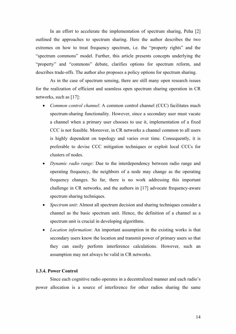
how large the reuse opportunity is. Figure 1-1 illustrates the setting for which

we want to quantify the reuse opportunity.

Figure 1-1. Links setting with marked signals.

• Can better transmitter-receiver placement setting provide more of this

particular reuse opportunity? In a way, the transmitter-receiver placement will

affect the propagation condition and interference, thus affecting the reuse

opportunity.

• Can we detect this particular reuse opportunity? Further, can smarter sensing

algorithm give better reuse opportunity detection or utilization? This will

depend on the sensing strategy that we employ.

The end-results will give a general understanding on the effect of different

indoor environment types, placement setting, and sensing strategies on the quantity

and visibility of the spectrum reuse opportunities, respectively. We further hope to

assess the kind of possible application of this cognitive radio system in an indoor

environment based on those understanding.

To answer the questions mentioned above and to obtain the end-results, this

work will closely follow the structure used in [3]. The main difference between this

17

work and [3] is that this work will focus on the indoor environments whereas [3]

focused on the outdoor environments. We note the similarities between this work and

the work in [3]:

a. This work also uses power-based primary transmitter detection with different

pre-determined single sensing threshold (an idealized version of primary

transmitter energy detection [7]).

b. This work also uses the same various sensing strategies with distributed power

control scheme applied in some cases.

Investigating how different transmitter-receiver placement setting may affect the

reuse opportunity is a new contribution of this thesis work.

1.5 Research method

For this thesis work, it is imperative to do a simulation that can represent the

“real life” condition as close as possible. This thesis work will follow the method and

approach used in [3], albeit with some adjustment since this work will focus on indoor

environments. In a synthetic indoor environment, we randomly generate two identical

primary and secondary systems (both consist of their respective primary and

secondary transmitter and receiver). To answer the questions stated in the problem

definition, we will want to look at the case where a primary link is active during the

sensing process of the secondary transmitter. By employing different sensing

schemes, we are interested in the successful transmission of both the primary and

secondary links, marked when both links achieve their required SINR. The limiting

value of this success probability corresponds to the actual reuse opportunities, thereby

providing an attempt to answer the earlier question(s) stated in the problem definition.

The use of a representative indoor propagation model is important to give a realistic

account of the required SINR calculation, which will give a coarse estimation on how

much overall reuse opportunity is available. We will describe the details of the

simulation in Chapter 3 of this report.

1.6 Thesis outline

This report is consisted of four chapters. The content of each chapter will be as

follows:

18

• Chapter 1: Introduction

This chapter will inform the reader about the background of the thesis work,

the aim of the work, related works, problem definition, research method, and

the thesis outline.

• Chapter 2: Simulation Model

This chapter will describe the system model, indoor propagation model,

various sensing strategies and placement settings, the performance measures

used, assumptions made for and used in the simulation, and the simulation

chain or path of the simulation in general.

• Chapter 3: Simulation Results and Analysis

This chapter will provide simulation results and the analysis/discussion for

each result, i.e. providing possible explanation for important simulation

outcome.

• Chapter 4: Conclusion and Future Work

This chapter will contain the conclusion of the thesis work, specifically about

the simulation results. Some suggestions of possible future works regarding

the same field/subject will also be available here.

19

CHAPTER 2

MODELS

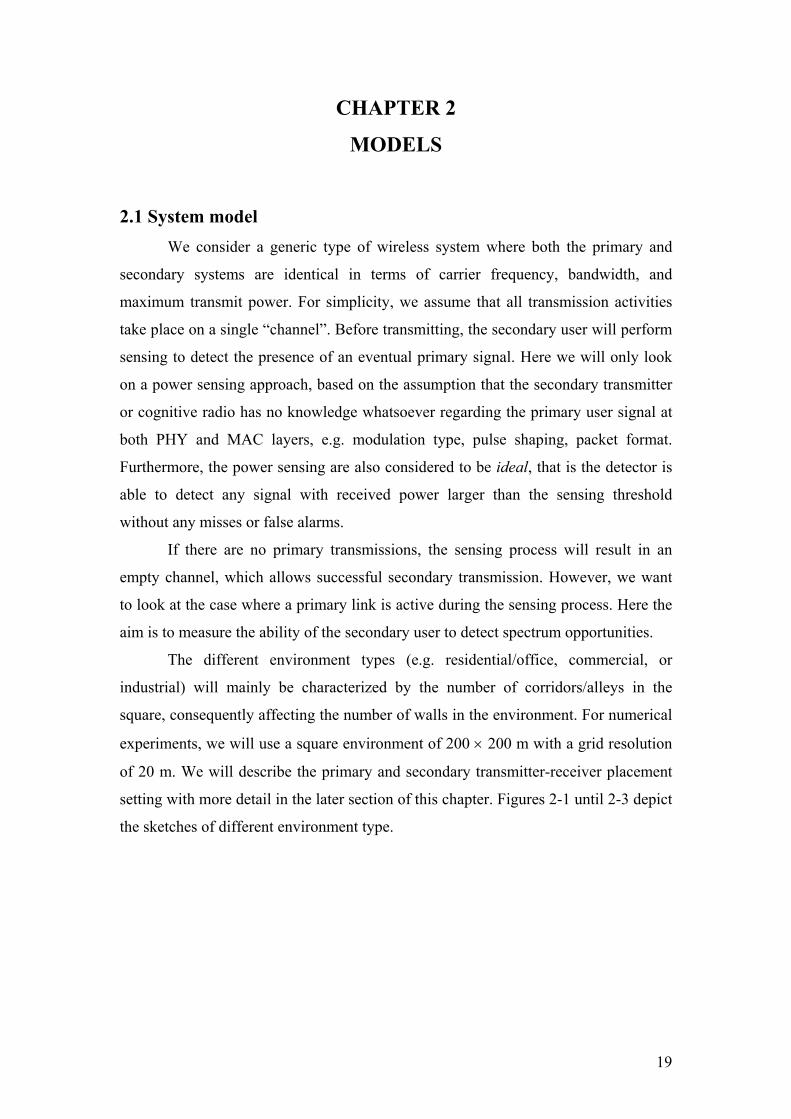
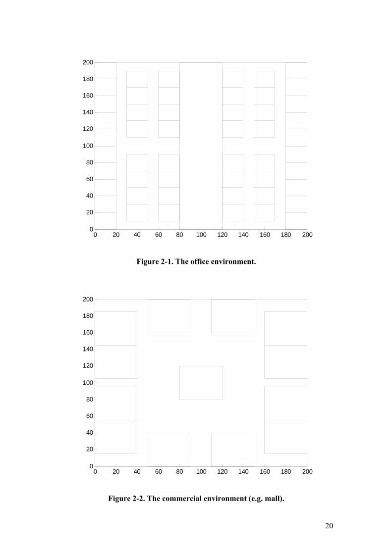
2.1 System model We consider a generic type of wireless system where both the primary and

secondary systems are identical in terms of carrier frequency, bandwidth, and

maximum transmit power. For simplicity, we assume that all transmission activities

take place on a single “channel”. Before transmitting, the secondary user will perform

sensing to detect the presence of an eventual primary signal. Here we will only look

on a power sensing approach, based on the assumption that the secondary transmitter

or cognitive radio has no knowledge whatsoever regarding the primary user signal at

both PHY and MAC layers, e.g. modulation type, pulse shaping, packet format.

Furthermore, the power sensing are also considered to be ideal, that is the detector is

able to detect any signal with received power larger than the sensing threshold

without any misses or false alarms.

If there are no primary transmissions, the sensing process will result in an

empty channel, which allows successful secondary transmission. However, we want

to look at the case where a primary link is active during the sensing process. Here the

aim is to measure the ability of the secondary user to detect spectrum opportunities.

The different environment types (e.g. residential/office, commercial, or

industrial) will mainly be characterized by the number of corridors/alleys in the

square, consequently affecting the number of walls in the environment. For numerical

experiments, we will use a square environment of 200 × 200 m with a grid resolution

of 20 m. We will describe the primary and secondary transmitter-receiver placement

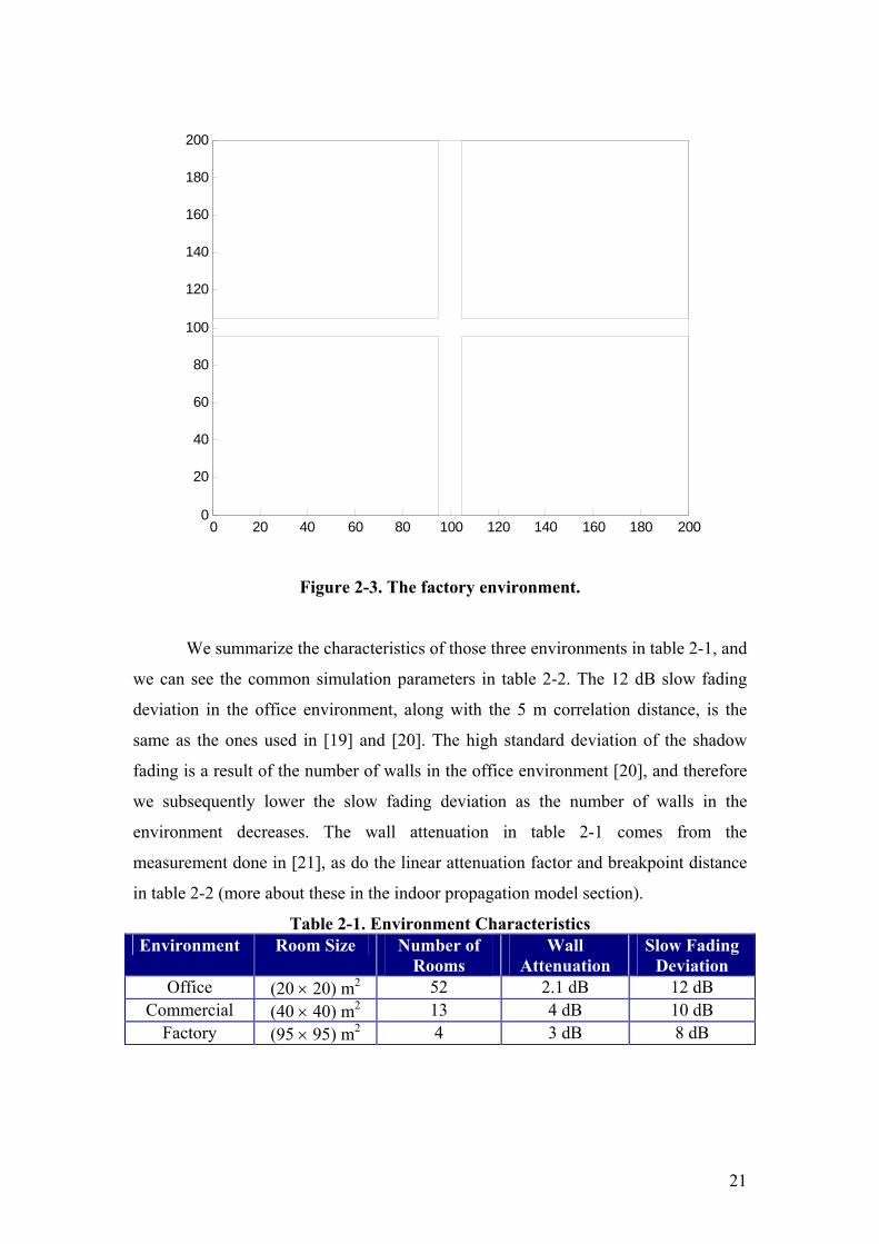
setting with more detail in the later section of this chapter. Figures 2-1 until 2-3 depict

the sketches of different environment type.

20

0 20 40 60 80 100 120 140 160 180 2000

20

40

60

80

100

120

140

160

180

200

Figure 2-1. The office environment.

0 20 40 60 80 100 120 140 160 180 2000

20

40

60

80

100

120

140

160

180

200

Figure 2-2. The commercial environment (e.g. mall).

21

0 20 40 60 80 100 120 140 160 180 2000

20

40

60

80

100

120

140

160

180

200

Figure 2-3. The factory environment.

We summarize the characteristics of those three environments in table 2-1, and

we can see the common simulation parameters in table 2-2. The 12 dB slow fading

deviation in the office environment, along with the 5 m correlation distance, is the

same as the ones used in [19] and [20]. The high standard deviation of the shadow

fading is a result of the number of walls in the office environment [20], and therefore

we subsequently lower the slow fading deviation as the number of walls in the

environment decreases. The wall attenuation in table 2-1 comes from the

measurement done in [21], as do the linear attenuation factor and breakpoint distance

in table 2-2 (more about these in the indoor propagation model section).

Table 2-1. Environment Characteristics Environment Room Size Number of

Rooms Wall

Attenuation Slow Fading

Deviation Office (20 × 20) m2 52 2.1 dB 12 dB

Commercial (40 × 40) m2 13 4 dB 10 dB Factory (95 × 95) m2 4 3 dB 8 dB

22

Table 2-2. Common Simulation Parameters Parameters Value

Maximum transmit power 1 mW = 0 dBm Minimum required SINR 10 dB

Noise level -120 dBm Carrier frequency 900 MHz

Linear attenuation factor (Γ) 0.2 dB/m [21] Breakpoint distance (dl) 65 m [21]

Slow fading correlation distance 5 m [19]

2.2 Indoor propagation model The nature of this thesis work results in the need to review literatures

regarding indoor propagation model ([21] – [29]). In this work, we will compute the

path-losses in figure 2-4 using the model in [21], which is an extended version of

Keenan-Motley (KM) model. The choice is made not only because the simplicity of

the model, but also because the measurement data used to construct the model was

taken in buildings that bear much resemblances with the environment described in

section 2.1. The complete expression used for the path-loss model is:

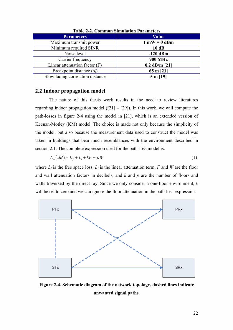
( )m f lL dB L L kF pW= + + + (1)

where Lf is the free space loss, Ll is the linear attenuation term, F and W are the floor

and wall attenuation factors in decibels, and k and p are the number of floors and

walls traversed by the direct ray. Since we only consider a one-floor environment, k

will be set to zero and we can ignore the floor attenuation in the path-loss expression.

Figure 2-4. Schematic diagram of the network topology, dashed lines indicate

unwanted signal paths.

23

The first part of the path-loss model is the free space loss, which has the

expression:

420 logfdL π

λ⎛ ⎞= ⋅ ⎜ ⎟⎝ ⎠

(2)

where λ is the wavelength and d is the transmitter-receiver separation (Tx-Rx

distance) in meters.

The second part of the path-loss model is the linear attenuation term, which

describes the LOS path-loss range dependence observed for large Tx-Rx separations

in some buildings [21]. The linear attenuation term has the expression:

[ ]0,l lL Max d d= Γ ⋅ − (3)

where Γ is the linear attenuation factor (expressed in dB/m), and dl is the Tx-Rx

separation where the linear attenuation starts, i.e. the breakpoint distance.

We note that this extended KM model can only describe the correlation

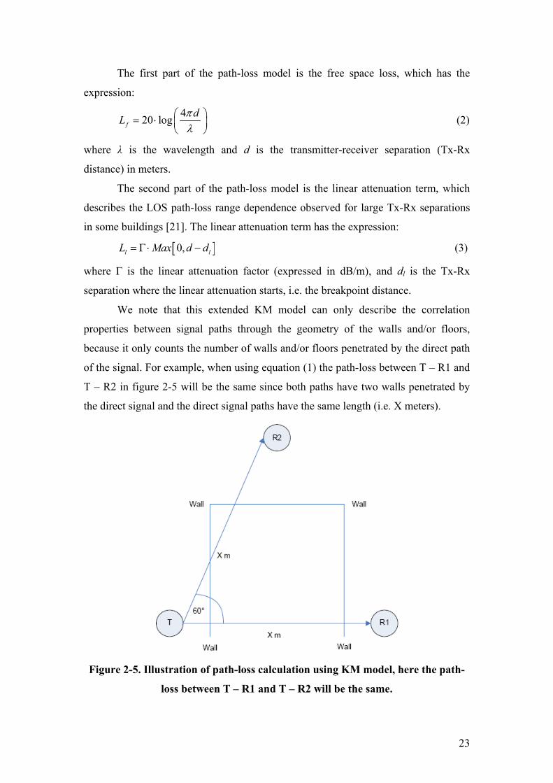
properties between signal paths through the geometry of the walls and/or floors,

because it only counts the number of walls and/or floors penetrated by the direct path

of the signal. For example, when using equation (1) the path-loss between T – R1 and

T – R2 in figure 2-5 will be the same since both paths have two walls penetrated by

the direct signal and the direct signal paths have the same length (i.e. X meters).

Figure 2-5. Illustration of path-loss calculation using KM model, here the path-

loss between T – R1 and T – R2 will be the same.

24

For a better representation of the indoor propagation, we add a shadow fading

process to the propagation model. We can model the shadow fading process in

different ways. The work in [20] uses a simple propagation model where the shadow

fading process is uncorrelated. Another work in [19] regarded the shadow fading as a

correlated process with a certain correlation distance.

We think that a correlated shadow fading process is more realistic since the

shadow fading for the same radio link at the nearby locations will not change very

much. Further, for the radio links that has similar propagation path, the shadow fading

experienced by each of them will not have much difference either [30]. To take into

account this correlation property, we use a rather simplified model of a correlation

filter to filter the uncorrelated fading process. We use the following autoregressive

filter model:

( )2

11

1

1

d

d

eH ze z

−

− −

−=

⎛ ⎞− ⎜ ⎟⎝ ⎠

(4)

The filter will produce an exponentially correlated fading process with e-1 decay at the

correlation distance d (the autocorrelation function of the fading process decays to e-1

of the maximum after a correlation distance of d) [31].

Therefore, the final propagation model that we use is:

( ) ( )m f lL dB L L pW h s= + + + (5)

where s is an uncorrelated lognormal distribution fading process with mean 0 and

standard deviation σ (see table 3-1), and h(s) is the correlated fading process as result

of the filtering.

2.3 Sensing and spectrum access strategies

Here we are not interested in the implementation detail; hence, we will assume

that all secondary transmitters can perform ideal power sensing with threshold κ, i.e.

the detector is able to detect any signal with received power larger than κ without any

misses or false alarms. If the secondary transmitter senses the channel to be clear, i.e.

the received power is below the sensing threshold, it will begin transmission attempt.

Finally, we also assume that the secondary transmitter knows the path-loss of STx –

SRx, and all other path gains are unknown. We will compare the performance of the

four following sensing strategies [3]:

25

A. Transmitter sensing – silent receiver (TX sensing)

Here the secondary transmitter has no knowledge regarding the presence of

the primary receiver. The secondary transmitter senses the channel and if it is

unable to detect the primary transmitter on the path PTx – STx it will start

transmission attempt. We will consider constant transmit power and an

adjusted transmit power mode that will result in the SNR at the secondary

receiver to be kγ0S in the absence of primary transmitter interference, where k

is the interference margin and γ0S is the minimum required SNR at the

secondary receiver.

B. Transmitter and receiver sensing (TX&RX sensing)

Here we assume that the secondary transmitter is able to detect the primary

receiver whenever propagation conditions allow the detection to happen, e.g.

by sensing return channel traffic such as CTS (clear-to-send) signal. The

secondary transmitter will not attempt transmission if it senses activity in

either the PTx – STx path or PRx – STx path, i.e. it will not use the channel.

We also consider two transmit power as mentioned in strategy A.

C. Responsive system, both transmitters using distributed power control (DPC)

In the previous cases, the primary system cannot mitigate the effect of

increased interference from the secondary transmitter, and vice versa. Here we

assume that both the primary and secondary transmitters adjust their power

according to a distributed power control (DPC) scheme. We assume success in

accessing channel if there exists a power setting (within the maximum power

limits) such that both the primary and secondary link achieve their respective

SINR target [32].

D. Collaborative sensing

Here the secondary transmitter gets additional sensing information from N

other cognitive radios in the network. We will model these as uniformly

distributed over the square using the same sensing threshold as the secondary

transmitter. If none of these devices detects any signal above the threshold

then the secondary user will attempt to access the channel (again considering

two transmit power as in strategy A and B).

26

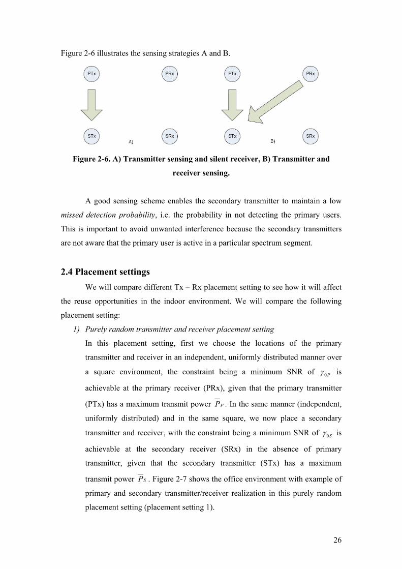
Figure 2-6 illustrates the sensing strategies A and B.

Figure 2-6. A) Transmitter sensing and silent receiver, B) Transmitter and

receiver sensing.

A good sensing scheme enables the secondary transmitter to maintain a low

missed detection probability, i.e. the probability in not detecting the primary users.

This is important to avoid unwanted interference because the secondary transmitters

are not aware that the primary user is active in a particular spectrum segment.

2.4 Placement settings

We will compare different Tx – Rx placement setting to see how it will affect

the reuse opportunities in the indoor environment. We will compare the following

placement setting:

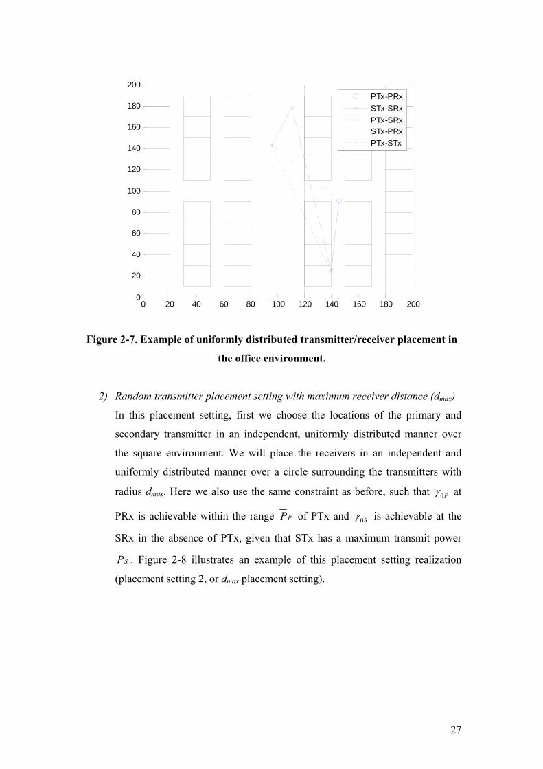
1) Purely random transmitter and receiver placement setting

In this placement setting, first we choose the locations of the primary

transmitter and receiver in an independent, uniformly distributed manner over

a square environment, the constraint being a minimum SNR of 0Pγ is

achievable at the primary receiver (PRx), given that the primary transmitter

(PTx) has a maximum transmit power PP . In the same manner (independent,

uniformly distributed) and in the same square, we now place a secondary

transmitter and receiver, with the constraint being a minimum SNR of 0Sγ is

achievable at the secondary receiver (SRx) in the absence of primary

transmitter, given that the secondary transmitter (STx) has a maximum

transmit power SP . Figure 2-7 shows the office environment with example of

primary and secondary transmitter/receiver realization in this purely random

placement setting (placement setting 1).

27

0 20 40 60 80 100 120 140 160 180 2000

20

40

60

80

100

120

140

160

180

200PTx-PRxSTx-SRxPTx-SRxSTx-PRxPTx-STx

Figure 2-7. Example of uniformly distributed transmitter/receiver placement in

the office environment.

2) Random transmitter placement setting with maximum receiver distance (dmax)

In this placement setting, first we choose the locations of the primary and

secondary transmitter in an independent, uniformly distributed manner over

the square environment. We will place the receivers in an independent and

uniformly distributed manner over a circle surrounding the transmitters with

radius dmax. Here we also use the same constraint as before, such that 0Pγ at

PRx is achievable within the range PP of PTx and 0Sγ is achievable at the

SRx in the absence of PTx, given that STx has a maximum transmit power

SP . Figure 2-8 illustrates an example of this placement setting realization

(placement setting 2, or dmax placement setting).

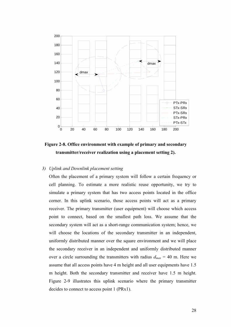
28

0 20 40 60 80 100 120 140 160 180 2000

20

40

60

80

100

120

140

160

180

200

PTx-PRxSTx-SRxPTx-SRxSTx-PRxPTx-STx

dmax

dmax

Figure 2-8. Office environment with example of primary and secondary

transmitter/receiver realization using a placement setting 2).

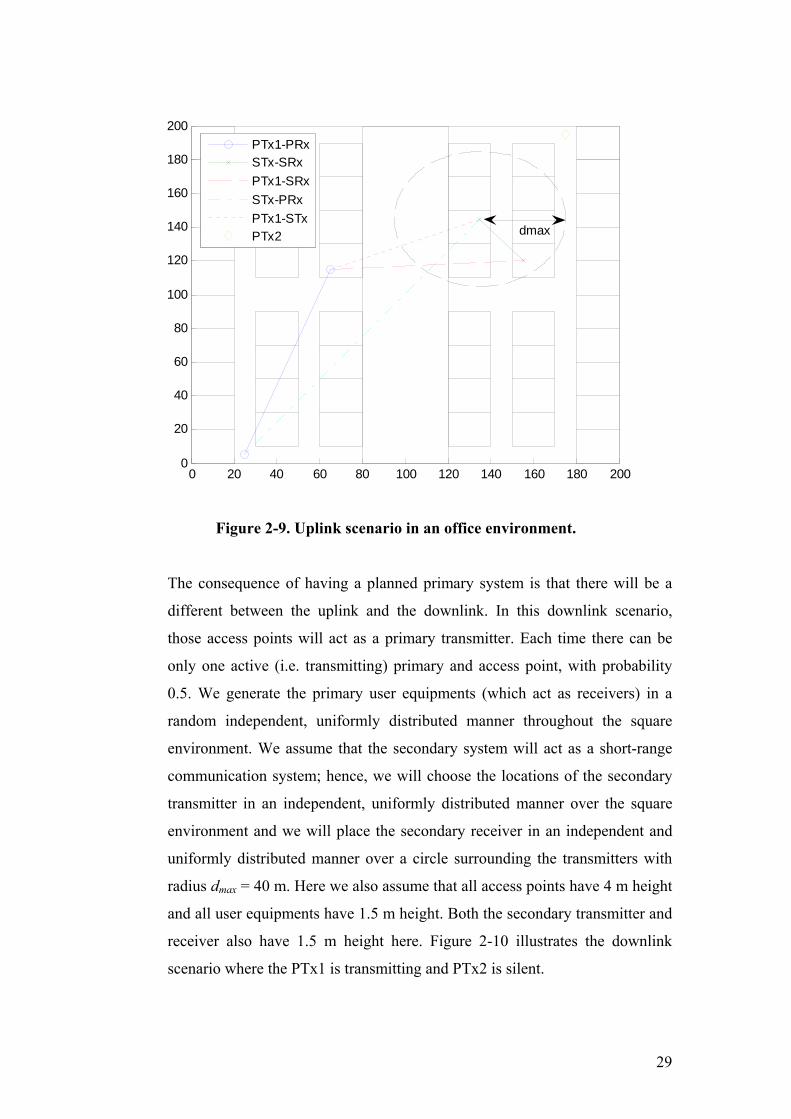
3) Uplink and Downlink placement setting

Often the placement of a primary system will follow a certain frequency or

cell planning. To estimate a more realistic reuse opportunity, we try to

simulate a primary system that has two access points located in the office

corner. In this uplink scenario, those access points will act as a primary

receiver. The primary transmitter (user equipment) will choose which access

point to connect, based on the smallest path loss. We assume that the

secondary system will act as a short-range communication system; hence, we

will choose the locations of the secondary transmitter in an independent,

uniformly distributed manner over the square environment and we will place

the secondary receiver in an independent and uniformly distributed manner

over a circle surrounding the transmitters with radius dmax = 40 m. Here we

assume that all access points have 4 m height and all user equipments have 1.5

m height. Both the secondary transmitter and receiver have 1.5 m height.

Figure 2-9 illustrates this uplink scenario where the primary transmitter

decides to connect to access point 1 (PRx1).

29

0 20 40 60 80 100 120 140 160 180 2000

20

40

60

80

100

120

140

160

180

200PTx1-PRxSTx-SRxPTx1-SRxSTx-PRxPTx1-STxPTx2 dmax

Figure 2-9. Uplink scenario in an office environment.

The consequence of having a planned primary system is that there will be a

different between the uplink and the downlink. In this downlink scenario,

those access points will act as a primary transmitter. Each time there can be

only one active (i.e. transmitting) primary and access point, with probability

0.5. We generate the primary user equipments (which act as receivers) in a

random independent, uniformly distributed manner throughout the square

environment. We assume that the secondary system will act as a short-range

communication system; hence, we will choose the locations of the secondary

transmitter in an independent, uniformly distributed manner over the square

environment and we will place the secondary receiver in an independent and

uniformly distributed manner over a circle surrounding the transmitters with

radius dmax = 40 m. Here we also assume that all access points have 4 m height

and all user equipments have 1.5 m height. Both the secondary transmitter and

receiver also have 1.5 m height here. Figure 2-10 illustrates the downlink

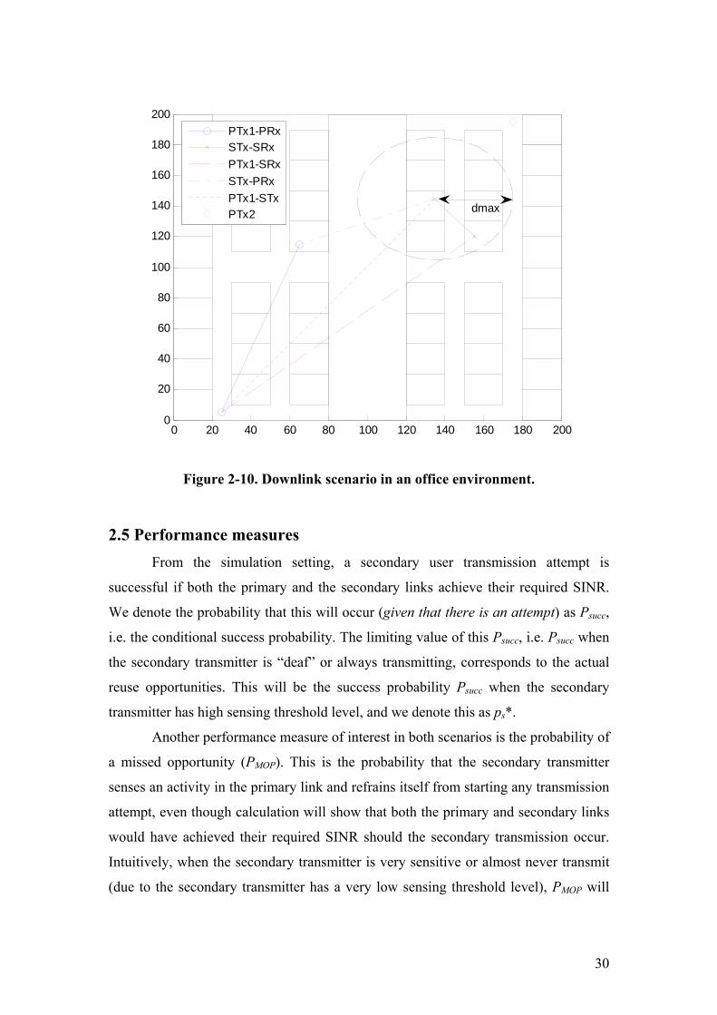
scenario where the PTx1 is transmitting and PTx2 is silent.

30

0 20 40 60 80 100 120 140 160 180 2000

20

40

60

80

100

120

140

160

180

200PTx1-PRxSTx-SRxPTx1-SRxSTx-PRxPTx1-STxPTx2 dmax

Figure 2-10. Downlink scenario in an office environment.

2.5 Performance measures

From the simulation setting, a secondary user transmission attempt is

successful if both the primary and the secondary links achieve their required SINR.

We denote the probability that this will occur (given that there is an attempt) as Psucc,

i.e. the conditional success probability. The limiting value of this Psucc, i.e. Psucc when

the secondary transmitter is “deaf” or always transmitting, corresponds to the actual

reuse opportunities. This will be the success probability Psucc when the secondary

transmitter has high sensing threshold level, and we denote this as ps*.

Another performance measure of interest in both scenarios is the probability of

a missed opportunity (PMOP). This is the probability that the secondary transmitter

senses an activity in the primary link and refrains itself from starting any transmission

attempt, even though calculation will show that both the primary and secondary links

would have achieved their required SINR should the secondary transmission occur.

Intuitively, when the secondary transmitter is very sensitive or almost never transmit

(due to the secondary transmitter has a very low sensing threshold level), PMOP will

31

converge to ps*, since at this condition all reuse opportunity will be a missed

opportunity.

Since we are interested in exploring the role of sensing strategy in detecting

reuse opportunities, the probability of finding a “clear” channel, i.e. not sensing the

primary transmitter (Pclear), can also be a performance measure of interest. The value

of Pclear can help determine the actual success probability, which will be lower than

Psucc, since Psucc is conditional success probability given that the secondary user

makes a transmission attempt. We can determine the actual success probability as

Pclear × Psucc.

2.6 Simulation chain

We describe the chain or path of the simulation in the simulation flowchart,

illustrated in Appendix A. In a way, the flowchart also tells on how various aspects

(e.g. environments, transmitter-receiver placements, indoor propagation model,

sensing strategies, and performance measures) come into play and interact in the

simulation sequence.

32

CHAPTER 3

SIMULATION RESULTS AND ANALYSIS

By means of simulation, we derive the following numerical results for three

different indoor environments. To allow for accurate comparisons between schemes,

we derive the results with the same random primary and secondary

transmitter/receiver locations in each simulated environment. Here we obtain each

presented results from 20,000 samples.

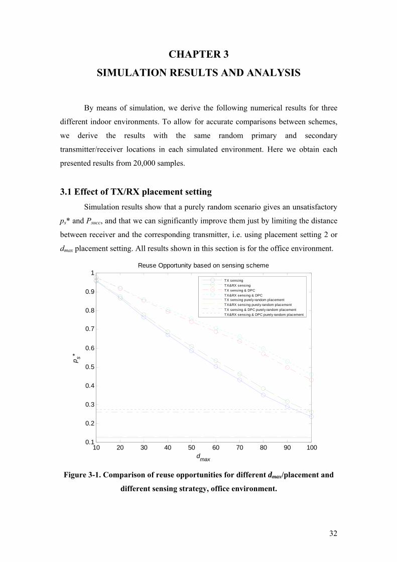
3.1 Effect of TX/RX placement setting

Simulation results show that a purely random scenario gives an unsatisfactory

ps* and Psucc, and that we can significantly improve them just by limiting the distance

between receiver and the corresponding transmitter, i.e. using placement setting 2 or

dmax placement setting. All results shown in this section is for the office environment.

10 20 30 40 50 60 70 80 90 1000.1

0.2

0.3

0.4

0.5

0.6

0.7

0.8

0.9

1

dmax

p s*

Reuse Opportunity based on sensing scheme

TX sensingTX&RX sensingTX sensing & DPCTX&RX sensing & DPCTX sensing purely random placementTX&RX sensing purely random placementTX sensing & DPC purely random placementTX&RX sensing & DPC purely random placement

Figure 3-1. Comparison of reuse opportunities for different dmax/placement and

different sensing strategy, office environment.

33

Figure 3-1 compares the obtained reuse opportunities for different

dmax/placement and different sensing strategy in an office environment. The lines

without marker in the lower part of the figure indicate ps* for a purely random TX/RX

placement setting when using different sensing strategy. This ps* corresponds to the

actual reuse opportunity, i.e. the probability that a randomly chosen secondary link

can coexist with the primary link in the given square environment. We observe ps* as

PMOP when Pclear approaches zero, or as Psucc when Pclear approaches one.

From the figure, we observe that both ps* become higher as dmax becomes

shorter, and they become lower as dmax becomes longer. Even when using a simple

sensing strategy, ps* can be very close to one when dmax is only 10 m. This is because

as dmax gets shorter, the receiver becomes closer to the corresponding transmitter, to

the extent that it is more likely that the location of the receiver is only in the next

room or the room after that. The proximity between a corresponding transmitter and

receiver is very close when compared to the longer distance between primary and

secondary transmitter. As such, this situation results in better interference protection

for both the primary and secondary receiver. Naturally, when a room encloses the

primary transmitter and receiver, and another room that is far away and shielded by

numerous walls between them encloses the secondary transmitter and receiver, each

receiver will have good protection from unwanted interference. We observe that ps*

goes to one regardless of the sensing strategy used when dmax goes to zero (which

means the corresponding transmitter and receiver will be located in the same room but

far separated from the other link, i.e. the other transmitter and receiver). These results

indicate that the cognitive radio system may be suitable for a short-range

communication system (e.g. between rooms in an office building).

We may conclude that ps* will greatly improve as we limit the distance of

receiver from the corresponding transmitter (dmax). As dmax goes to zero, ps* goes to

one, and the role of advance sensing strategy becomes less significant (for dmax = 10 m

ps* remains relatively unchanged regardless of the used sensing strategy). Hence, the

choice of what sensing strategy to use may depend on the minimum ps* that the

provider/regulator will pursue and/or limitation of dmax that the link provider/regulator

will impose. For example, if we want to pursue a minimum ps* of 0.5, then it is

sufficient to use TX sensing up to dmax = 60 m (alternatively, if dmax is limited to 60 m

it is sufficient to use TX sensing to obtain a minimum ps* of 0.5). If we increase dmax,

we will need to employ an advanced sensing strategy to maintain the level of ps*, e.g.

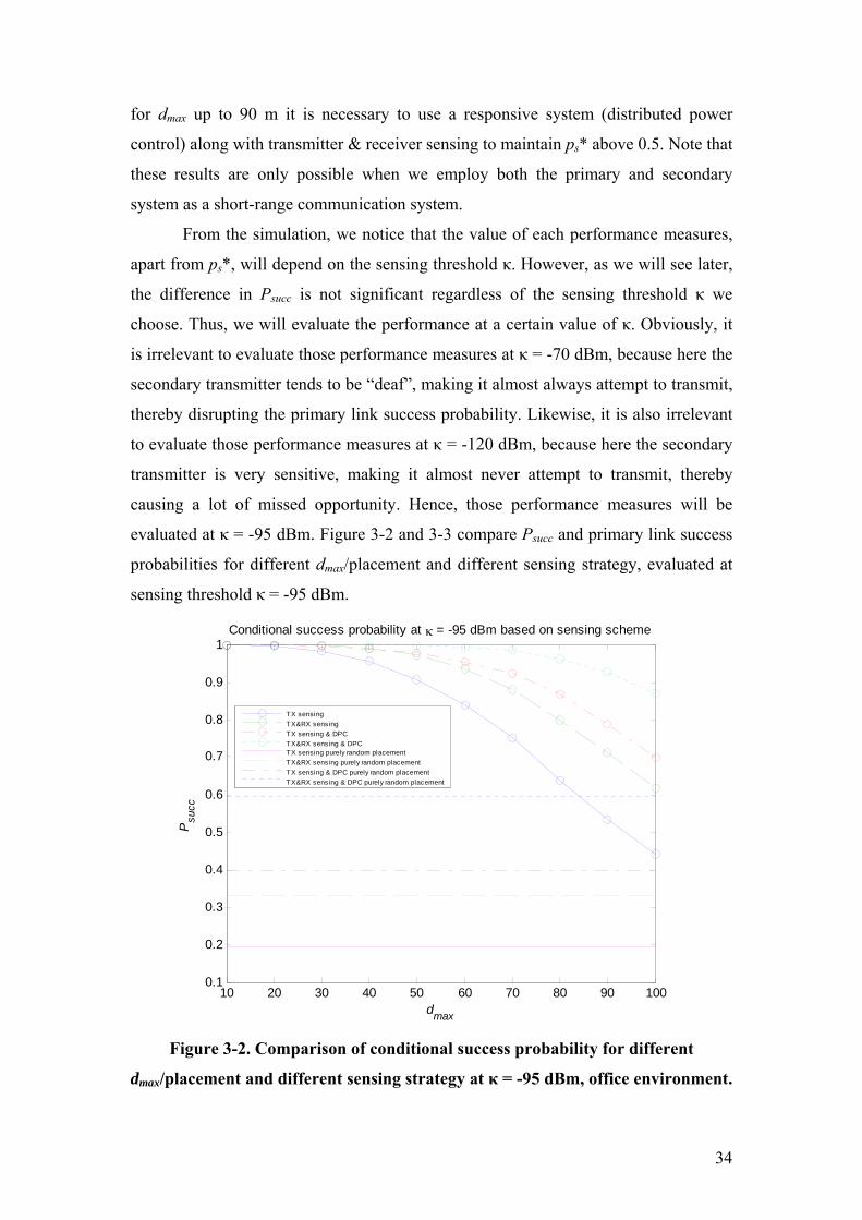
34

for dmax up to 90 m it is necessary to use a responsive system (distributed power

control) along with transmitter & receiver sensing to maintain ps* above 0.5. Note that

these results are only possible when we employ both the primary and secondary

system as a short-range communication system.

From the simulation, we notice that the value of each performance measures,

apart from ps*, will depend on the sensing threshold κ. However, as we will see later,

the difference in Psucc is not significant regardless of the sensing threshold κ we

choose. Thus, we will evaluate the performance at a certain value of κ. Obviously, it

is irrelevant to evaluate those performance measures at κ = -70 dBm, because here the

secondary transmitter tends to be “deaf”, making it almost always attempt to transmit,

thereby disrupting the primary link success probability. Likewise, it is also irrelevant

to evaluate those performance measures at κ = -120 dBm, because here the secondary

transmitter is very sensitive, making it almost never attempt to transmit, thereby

causing a lot of missed opportunity. Hence, those performance measures will be

evaluated at κ = -95 dBm. Figure 3-2 and 3-3 compare Psucc and primary link success

probabilities for different dmax/placement and different sensing strategy, evaluated at

sensing threshold κ = -95 dBm.

10 20 30 40 50 60 70 80 90 1000.1

0.2

0.3

0.4

0.5

0.6

0.7

0.8

0.9

1

dmax

Psu

cc

Conditional success probability at κ = -95 dBm based on sensing scheme


Figure 3-2. Comparison of conditional success probability for different

dmax/placement and different sensing strategy at κ = -95 dBm, office environment.

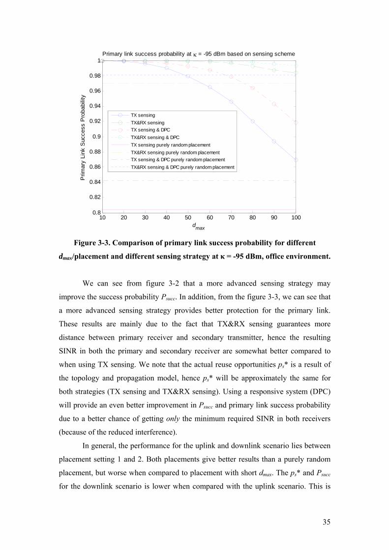
35

10 20 30 40 50 60 70 80 90 1000.8

0.82

0.84

0.86

0.88

0.9

0.92

0.94

0.96

0.98

1

dmax

Prim

ary

Link

Suc

cess

Pro

babi

lity

Primary link success probability at κ = -95 dBm based on sensing scheme


Figure 3-3. Comparison of primary link success probability for different

dmax/placement and different sensing strategy at κ = -95 dBm, office environment.

We can see from figure 3-2 that a more advanced sensing strategy may

improve the success probability Psucc. In addition, from the figure 3-3, we can see that

a more advanced sensing strategy provides better protection for the primary link.

These results are mainly due to the fact that TX&RX sensing guarantees more

distance between primary receiver and secondary transmitter, hence the resulting

SINR in both the primary and secondary receiver are somewhat better compared to

when using TX sensing. We note that the actual reuse opportunities ps* is a result of

the topology and propagation model, hence ps* will be approximately the same for

both strategies (TX sensing and TX&RX sensing). Using a responsive system (DPC)

will provide an even better improvement in Psucc and primary link success probability

due to a better chance of getting only the minimum required SINR in both receivers

(because of the reduced interference).

In general, the performance for the uplink and downlink scenario lies between

placement setting 1 and 2. Both placements give better results than a purely random

placement, but worse when compared to placement with short dmax. The ps* and Psucc

for the downlink scenario is lower when compared with the uplink scenario. This is

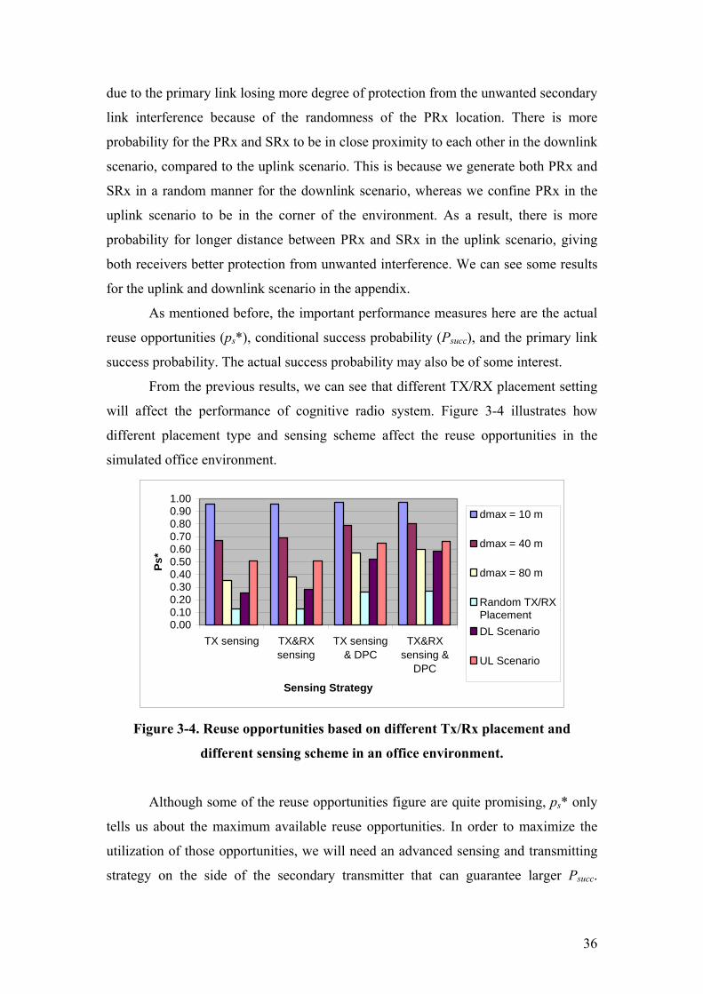
36

due to the primary link losing more degree of protection from the unwanted secondary

link interference because of the randomness of the PRx location. There is more

probability for the PRx and SRx to be in close proximity to each other in the downlink

scenario, compared to the uplink scenario. This is because we generate both PRx and

SRx in a random manner for the downlink scenario, whereas we confine PRx in the

uplink scenario to be in the corner of the environment. As a result, there is more

probability for longer distance between PRx and SRx in the uplink scenario, giving

both receivers better protection from unwanted interference. We can see some results

for the uplink and downlink scenario in the appendix.

As mentioned before, the important performance measures here are the actual

reuse opportunities (ps*), conditional success probability (Psucc), and the primary link

success probability. The actual success probability may also be of some interest.

From the previous results, we can see that different TX/RX placement setting

will affect the performance of cognitive radio system. Figure 3-4 illustrates how

different placement type and sensing scheme affect the reuse opportunities in the

simulated office environment.

0.000.100.200.300.400.500.600.700.800.901.00

TX sensing TX&RXsensing

TX sensing& DPC

TX&RXsensing &

DPC

Sensing Strategy

Ps*

dmax = 10 m

dmax = 40 m

dmax = 80 m

Random TX/RXPlacementDL Scenario

UL Scenario

Figure 3-4. Reuse opportunities based on different Tx/Rx placement and

different sensing scheme in an office environment.

Although some of the reuse opportunities figure are quite promising, ps* only

tells us about the maximum available reuse opportunities. In order to maximize the

utilization of those opportunities, we will need an advanced sensing and transmitting

strategy on the side of the secondary transmitter that can guarantee larger Psucc.

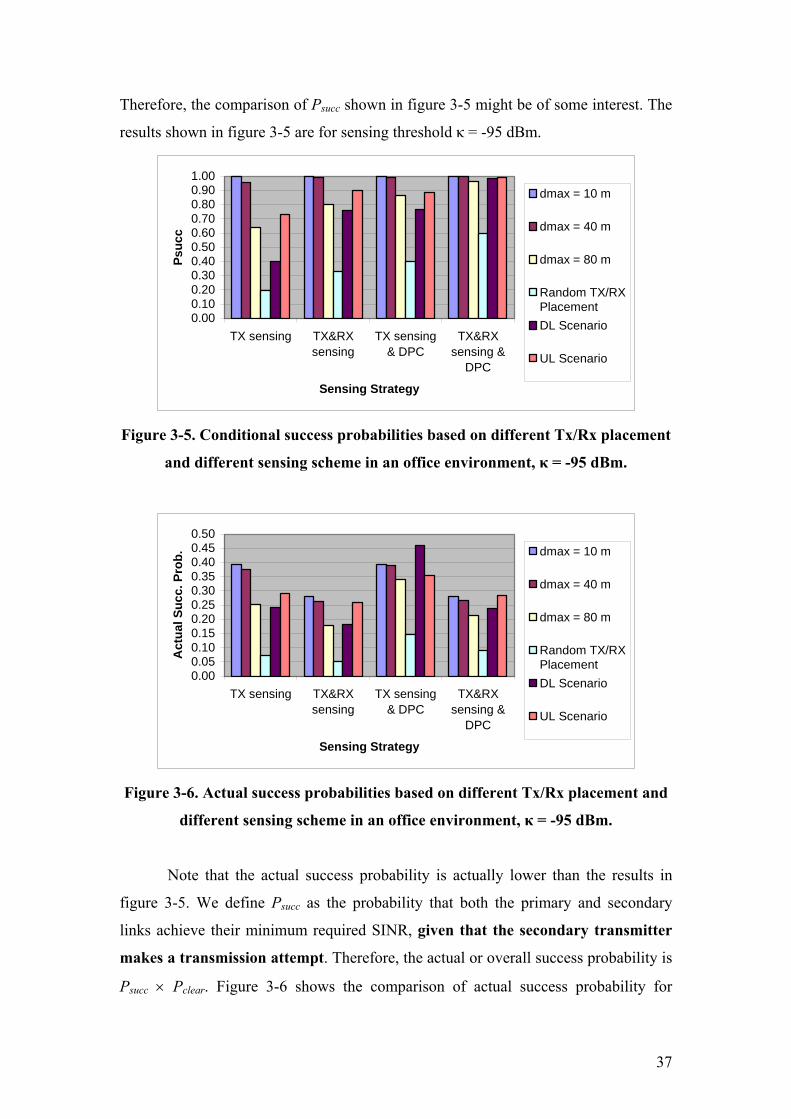
37

Therefore, the comparison of Psucc shown in figure 3-5 might be of some interest. The

results shown in figure 3-5 are for sensing threshold κ = -95 dBm.

0.000.100.200.300.400.500.600.700.800.901.00


TX sensing& DPC

TX&RXsensing &

DPC

Sensing Strategy

Psuc

cdmax = 10 m

dmax = 40 m

dmax = 80 m


UL Scenario

Figure 3-5. Conditional success probabilities based on different Tx/Rx placement

and different sensing scheme in an office environment, κ = -95 dBm.

0.000.050.100.150.200.250.300.350.400.450.50


TX sensing& DPC

TX&RXsensing &

DPC

Sensing Strategy

Act

ual S

ucc.

Pro

b. dmax = 10 m

dmax = 40 m

dmax = 80 m


UL Scenario

Figure 3-6. Actual success probabilities based on different Tx/Rx placement and

different sensing scheme in an office environment, κ = -95 dBm.

Note that the actual success probability is actually lower than the results in

figure 3-5. We define Psucc as the probability that both the primary and secondary

links achieve their minimum required SINR, given that the secondary transmitter

makes a transmission attempt. Therefore, the actual or overall success probability is

Psucc × Pclear. Figure 3-6 shows the comparison of actual success probability for

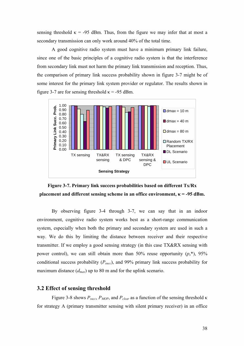
38

sensing threshold κ = -95 dBm. Thus, from the figure we may infer that at most a

secondary transmission can only work around 40% of the total time.

A good cognitive radio system must have a minimum primary link failure,

since one of the basic principles of a cognitive radio system is that the interference

from secondary link must not harm the primary link transmission and reception. Thus,

the comparison of primary link success probability shown in figure 3-7 might be of

some interest for the primary link system provider or regulator. The results shown in

figure 3-7 are for sensing threshold κ = -95 dBm.

0.000.100.200.300.400.500.600.700.800.901.00


TX sensing& DPC

TX&RXsensing &

DPC

Sensing Strategy

Prim

ary

Link

Suc

c. P

rob.

dmax = 10 m

dmax = 40 m

dmax = 80 m


UL Scenario

Figure 3-7. Primary link success probabilities based on different Tx/Rx

placement and different sensing scheme in an office environment, κ = -95 dBm.

By observing figure 3-4 through 3-7, we can say that in an indoor

environment, cognitive radio system works best as a short-range communication

system, especially when both the primary and secondary system are used in such a

way. We do this by limiting the distance between receiver and their respective

transmitter. If we employ a good sensing strategy (in this case TX&RX sensing with

power control), we can still obtain more than 50% reuse opportunity (ps*), 95%

conditional success probability (Psucc), and 99% primary link success probability for

maximum distance (dmax) up to 80 m and for the uplink scenario.

3.2 Effect of sensing threshold

Figure 3-8 shows Psucc, PMOP, and Pclear as a function of the sensing threshold κ

for strategy A (primary transmitter sensing with silent primary receiver) in an office

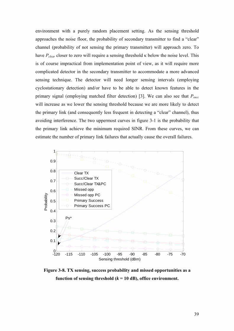
39

environment with a purely random placement setting. As the sensing threshold

approaches the noise floor, the probability of secondary transmitter to find a “clear”

channel (probability of not sensing the primary transmitter) will approach zero. To

have Pclear closer to zero will require a sensing threshold κ below the noise level. This

is of course impractical from implementation point of view, as it will require more

complicated detector in the secondary transmitter to accommodate a more advanced

sensing technique. The detector will need longer sensing intervals (employing

cyclostationary detection) and/or have to be able to detect known features in the

primary signal (employing matched filter detection) [3]. We can also see that Psucc

will increase as we lower the sensing threshold because we are more likely to detect

the primary link (and consequently less frequent in detecting a “clear” channel), thus

avoiding interference. The two uppermost curves in figure 3-1 is the probability that

the primary link achieve the minimum required SINR. From these curves, we can

estimate the number of primary link failures that actually cause the overall failures.

-120 -115 -110 -105 -100 -95 -90 -85 -80 -75 -700

0.1

0.2

0.3

0.4

0.5

0.6

0.7

0.8

0.9

1

Sensing threshold (dBm)

Pro

babi

lity

Clear TXSucc/Clear TXSucc/Clear TX&PCMissed oppMissed opp PCPrimary SuccessPrimary Success PC

Ps*

Figure 3-8. TX sensing, success probability and missed opportunities as a

function of sensing threshold (k = 10 dB), office environment.

40

The results in figure 3-8 are similar with the one in [3], which presented the

reuse opportunities in an outdoor environment scenario. From figure 3-8, we can see

that as we lower the sensing threshold, the increase in Psucc (the conditional success

probabilities given that a clear channel is sensed) is not significant. In this case,

sensing is not that helpful since the success probability is not really improving

compared to a “deaf” secondary transmitter. The secondary transmitter will become

more sensitive, thus avoiding more and more transmission attempt, as the sensing

threshold becomes lower. This causes an increase in the missed opportunity

probability, PMOP. When Pclear approaches zero, there will be no secondary

transmission at all, hence all reuse opportunities become missed opportunities. We

denote this limiting value of PMOP as ps*, which corresponds to the actual reuse

opportunities, i.e. the probability that a randomly chosen secondary link can coexist

with the primary link in the given square environment.

As the sensing threshold becomes higher, the secondary transmitter will

become more “deaf” toward primary transmission and will transmit more frequently.

When the threshold level is high enough that Pclear is close to one, the secondary

transmitter will always transmit and the success probability will converge/tend to ps*.

In figure 3-8, the sensing scheme with secondary transmitter power control is

using an interference margin of k = 10 dB. From the figure, we can infer that

employing secondary transmitter power control (which means not using more power

than necessary for the secondary transmitter) is not always beneficial to the reuse

opportunities and success probability. However, from the uppermost curve in the

figure we can also see that secondary transmitter power control may provide better

protection for the primary link. What happen here is because when we use k = 10 dB,

the received power in secondary receiver becomes less compared to when the

secondary transmitter is using maximum transmit power. Consequently, the secondary

receiver SINR is decreasing (causing lower Psucc) and the primary receiver SINR is

increasing (causing higher primary link success probability). We may also conclude

that choosing an optimum value of interference margin when employing a secondary

transmitter power control will be a trade-off between the overall Psucc (implicitly also

corresponds to PMOP) and primary link only success probability (protection for the

primary link).

Additional results in the appendix will show that collaborative sensing strategy

does not significantly improve the performance of cognitive radio system, especially

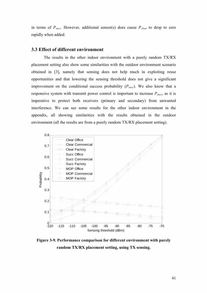
41

in terms of Psucc. However, additional sensor(s) does cause Pclear to drop to zero

rapidly when added.

3.3 Effect of different environment The results in the other indoor environment with a purely random TX/RX

placement setting also show some similarities with the outdoor environment scenario

obtained in [3], namely that sensing does not help much in exploiting reuse

opportunities and that lowering the sensing threshold does not give a significant

improvement on the conditional success probability (Psucc). We also know that a

responsive system with transmit power control is important to increase Psucc, as it is

imperative to protect both receivers (primary and secondary) from unwanted

interference. We can see some results for the other indoor environment in the

appendix, all showing similarities with the results obtained in the outdoor

environment (all the results are from a purely random TX/RX placement setting).

-120 -115 -110 -105 -100 -95 -90 -85 -80 -75 -700

0.1

0.2

0.3

0.4

0.5

0.6

0.7

0.8


Pro

babi

lity

Clear OfficeClear CommercialClear FactorySucc OfficeSucc CommercialSucc FactoryMOP OfficeMOP CommercialMOP Factory

Figure 3-9. Performance comparison for different environment with purely

random TX/RX placement setting, using TX sensing.

42

Figure 3-9 shows how different environment affects the performance of the

cognitive radio system. Here we show Psucc, PMOP, and Pclear for strategy A (primary

transmitter sensing with silent primary receiver). From the figure, we may see that

detecting a primary transmitter signal is easier in an environment with fewer walls

(corresponding to fewer rooms), in this case the factory environment. As the number

of walls (rooms) increases, detecting a primary transmitter signal will also become

harder. In contrast, success probability (Psucc) and reuse opportunity (ps*) is better in

an environment with more walls (rooms). The numerous walls (rooms) in the office

environment provide better protection against unwanted interference compared to the

other environment with fewer walls (rooms). Consequently, they also provide more

opportunity for coexistence between links when compared to other environment with

fewer walls (rooms). As before, the increase in Psucc is not significant when we lower

the sensing threshold.

43

CHAPTER 4

CONCLUSION AND FUTURE WORK

Simulation results showed that reuse opportunities are highly dependent on

TX/RX placement. For purely random placed transmitters and receivers, the system

performance in terms of the actual reuse opportunity (ps*) and conditional success

probability (Psucc) is proven to be unsatisfactory. In an office environment with a

purely random TX/RX placement, an advanced sensing strategy can achieve a reuse

opportunity as high as 27%, which is still relatively low. These ps* and Psucc can

improve significantly as we limit the distance of receiver from the corresponding

transmitter, i.e. by limiting dmax. Here ps* goes to one as dmax goes to zero, and even a

simple sensing strategy can give good ps* and Psucc for short dmax. From simulation, in

an office environment a simple TX sensing can give a minimum ps* of 50% for dmax

up to 60 m.

Through several type of placement setting/strategy, we concur that the system

(i.e. cognitive radio in indoor environment) works best as a short-range

communication system. We can obtain maximum reuse opportunity by combination

of careful transmitter and receiver placement, advanced sensing strategy, and

responsive transmitter. In this case, we obtain the maximum reuse opportunity when

we employ both primary and secondary system as a short-range communication

system while limiting their maximum distance. Simulation results showed that in an

office environment, TX&RX sensing with responsive system (transmit power control)

can give more than 50% ps*, 95% Psucc, and 99% primary link success probability

when using -95 dBm sensing threshold for dmax up to 80 m.

One drawback of this placement setting is that employing both primary and

secondary system as a short-range communication system may be impractical in real

life. A more acceptable implementation is to utilize the secondary system as a short-

range communication system inside a planned primary system cell/area, which still

gives an acceptable performance albeit only in the uplink.

The results also showed some similarities with outdoor simulation/scenario,

namely that sensing does not help much in exploiting reuse opportunities and that

lowering the sensing threshold does not give a significant improvement on Psucc.

Naturally, employing transmit power control may improve ps* and Psucc as it can

44

protect both the primary and secondary receivers from unwanted interference. Here

we also found environment dependence on the system performance, as an

environment with more walls makes detecting primary signal more difficult, but

provides more protection for unwanted interference, improving Psucc and ps*.

In this work, we use a rather simplified indoor propagation model. Future

work may include the use of a more realistic propagation model, such as ray tracing,

which can represent better correlation property between links. Another issue is the

implementation details of the sensing strategy. Here we employ an ideal sensing

which prevents any missed detection or false alarms. Future work should incorporate

these factors to see whether there are significant changes in the overall reuse

opportunity and success probability. Future work may also investigate the reuse

opportunity in a multi-floor building (e.g. if the primary and secondary system is

located on a different floor) and the effect of using higher/lower carrier frequency

towards the reuse opportunity in an indoor environment. Results from real time

measurement can also be of some interest for future works.

45

REFERENCES

[1] National Telecommunications and Information Administration (NTIA), “FCC

Frequency Allocation Chart,” 2003. Download available at

www.ntia.doc.gov/osmhome/allochrt.pdf.

[2] J.M. Peha, “Approaches to Spectrum Sharing,” IEEE Communications

Magazine, Vol. 43, Issue 2, pp. 10-12, February 2005.

[3] J. Zander, “Can We Find (And Use) “Spectrum Holes” In Real Life? – On The

Performance of Spectrum Sensing In “Cognitive” Radio Systems,” Invited

paper, IEEE Vehicular Technology Conference (VTC) spring 2009,

Barcelona, March 2009.

[4] S. Srinivasa, S. A. Jafar, “The Throughput Potential of Cognitive Radio: A

Theoretical Perspective,” Invited Paper, Fortieth Asilomar Conference on

Signals, Systems and Computers, 2006. pp. 221-225, 29 October – 1

November 2006.

[5] S. Srinivasa, S. A. Jafar, “The Throughput Potential of Cognitive Radio: A

Theoretical Perspective,” IEEE Communications Magazine, pp. 73-79, May

2007.

[6] S. A. Jafar, S. Srinivasa, “Capacity Limits of Cognitive Radio with Distributed

and Dynamic Spectral Activity,” IEEE Journal on Selected Areas in

Communications, vol. 25, pp. 529–537, April 2007.

[7] D. Cabric, S. M. Mishra, R. W. Brodersen, “Implementation Issues in

Spectrum Sensing for Cognitive Radios,” Thirty-Eighth Asilomar Conference

on Signals, Systems and Computers, 2004. Volume 1, pp. 772-776, 7-10

November 2004.

[8] S. Srinivasa, S. A. Jafar, “Soft Sensing and Optimal Power Control for

Cognitive Radio,” Proc. IEEE Globecom 2007.

[9] K. Hamdi, W. Zhang, K. Ben Letaief, “Power Control in Cognitive Radio

Systems Based on Spectrum Sensing Side Information,” IEEE International

Conference on Communications, June 2007.

[10] J. Unnikrishnan, V. V. Veeravalli, “Cooperative Sensing for Primary

Detection in Cognitive Radio,” IEEE Journal of Selected Topics in Signal

Processing, vol. 2, No. 1, pp. 18-27, February 2008.

46

[11] G. Ganesan, Y. Li, “Cooperative Spectrum Sensing in Cognitive Radio, Part I:

Two User Networks,” IEEE Transactions on Wireless Communications, vol.

6, No. 6, pp. 2204-2213, June 2007.

[12] H. Choi, K. Jang, Y. Cheong, “Adaptive Sensing Threshold Control Based on

Transmission Power in Cognitive Radio Systems,” Invited Paper, 3rd

International Conference on Cognitive Radio Oriented Wireless Networks and

Communications, 2008. CrownCom 2008. pp. 1-6, 15-17 May 2008.

[13] J. Zhu, Z. Xu, F. Wang, B. Huang, B. Zhang, “Double Threshold Energy

Detection of Cooperative Spectrum Sensing in Cognitive Radio,” 3rd

International Conference on Cognitive Radio Oriented Wireless Networks and

Communications, 2008. CrownCom 2008. pp. 1-5, 15-17 May 2008.

[14] M. Nekovee, “Impact of Cognitive Radio on Future Management of

Spectrum,” Invited Paper, 3rd International Conference on Cognitive Radio

Oriented Wireless Networks and Communications, 2008. CrownCom 2008.

pp. 1-6, 15-17 May 2008.

[15] M. Sherman, A. N. Mody, R. Martinez, C. Rodriguez, “IEEE Standards

Supporting Cognitive Radio and Networks, Dynamic Spectrum Access, and

Coexistence,” IEEE Communications Magazine, pp. 72-79, July 2008.

[16] J. Mitola, G. Q. Maguire, “Cognitive Radio: Making Software Radios More

Personal,” IEEE Personal Communications, vol. 6, no. 4, pp. 13-18, August

1999.

[17] I. F. Akyildiz, W. Lee, M. C. Vuran, S. Mohanty, “A Survey on Spectrum

Management in Cognitive Radio Networks,” IEEE Communications

Magazine, pp. 40-48, April 2008.

[18] C. Guo, T. Zhang, Z. Zeng, C. Feng, “Investigation on Spectrum Sharing

Technology Based on Cognitive Radio,” First International Conference on

Communications and Networking in China, 2006. ChinaCom '06. pp. 1-5, 25-

27 October 2006.

[19] 3rd Generation Partnership Project (3GPP); Technical Specification Group

Radio Access Network; FDD Base Station Classification (Release 2000). 3G

TR 25.951 V0.0.1 (2000-09); Technical Report.

[20] S. Pettersson, “Radio Resource Management for Wireless Indoor

Communication Systems: Performance and Implementation Aspects,” PhD

Dissertation, Radio Communication Systems Laboratory, Royal Institute of

47

Technology, 2004.

[21] C. Törnevik, J. Berg, F. Lotse, M. Madfors, “Propagation Models, Cell

Planning and Channel Allocation for Indoor Applications of Cellular

Systems,” IEEE 43rd Vehicular Technology Conference, 1993, pp. 867-870,

18-20 May 1993.

[22] M. Lott, I. Forkel, “A Multi-Wall-and-Floor Model for Indoor Radio

Propagation,” IEEE VTS 53rd Vehicular Technology Conference, 2001. VTC

2001 Spring. Volume 1, pp. 464-468, 6-9 May 2001.

[23] K. W. Cheung, J. H. Sau, M. S. Fong, R. D. Murch, “Indoor Propagation

Prediction Utilizing a New Empirical Model,” Singapore ICCS '94.

Conference Proceedings. Volume 1, pp. 15-19, 14-18 November 1994.

[24] S. Y. Seidel, T. S. Rappaport, ”900 MHz Path Loss Measurements and

Prediction Techniques for In-Building Communication System Design,” Proc.

41st IEEE Vehicular Technology Conf., pp. 613-618, May 1991.

[25] S. Y. Seidel, T. S. Rappaport, “914 MHz Path Loss Prediction Models for

Indoor Wireless Communications in Multifloored Buildings,” IEEE

Transactions on Antennas and Propagation, vol. 40, No. 2, pp. 207-217,

February 1992.

[26] S. Y. Seidel, T. S. Rappaport, M. J. Feuerstein, K. L. Blackard, “The impact of

surrounding buildings on propagation for wireless in-building personal

communications system design,” Proc. 42nd IEEE Vehicular Technology

Conference, pp. 814-818, May 1992.

[27] J. F. Lafortune, M. Lecours, “Measurement and Modeling of Propagation

Losses in a Building at 900 MHz,” IEEE Transactions on Vehicular

Technology, pp. 101-108, May 1990.

[28] J. Kivinen, X. Zhao, P. Vainikainen, “Wideband Indoor Radio Channel

Measurements With Direction of Arrival Estimations in the 5 GHz Band,”

IEEE VTS 50th Vehicular Technology Conference, 1999. VTC 1999 - Fall.

vol. 4, pp. 2308-2312, 19-22 September 1999.

[29] S. Zvhovec, M. Valek, P. Pechac, “Results of Indoor Propagation

Measurement Campaign For WLAN Systems Operating in 2.4 GHz ISM

Band,” Twelfth International Conference on Antennas and Propagation, 2003.

(ICAP 2003). vol. 1, pp. 63-66, 31 March-3 April 2003.

[30] IEEE C802.16m-07/060; F. I-Kang, L. Chi-Fang, S. Ting-Chen, S. Wern-Hoo,

48

“Correlation Models for Shadow Fading Simulation,” submitted on 5 March

2007 as part of IEEE 802.16 Broadband Wireless Access Working Group

Project, http://ieee802.org/16.

[31] Lecture Notes IK2502: Project Course in Wireless Networks, Year 2008.

[32] J. Zander, S. L. Kim, “Radio Resource Management in Wireless Networks,”

Artech House, 2001.

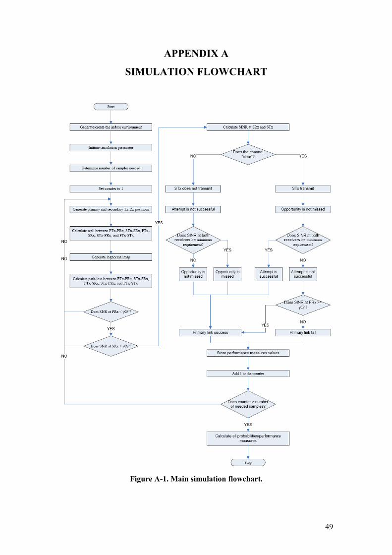
49

APPENDIX A

SIMULATION FLOWCHART

Figure A-1. Main simulation flowchart.

50

APPENDIX B

ADDITIONAL RESULTS

Figures B-1 show the results when using TX&RX sensing, i.e. the secondary

transmitter is also able to detect the primary receiver, in an office environment with

dmax = 40 m. From the figure, we can see that this strategy improves the ability to

detect the primary transmission and improves the success probability Psucc, although

somewhat only marginally. In addition, from the uppermost curve in figure 3-4, we

can see that this strategy provides better protection for the primary link. These results

are mainly due to the fact that TX&RX sensing guarantee more distance between

primary receiver and secondary transmitter, hence the resulting SINR in both the

primary and secondary receiver are somewhat better compared to when using TX

sensing. We note that the actual reuse opportunities ps* is a result of the topology and

propagation model, hence ps* will be approximately the same for TX sensing and

TX&RX sensing.

-120 -115 -110 -105 -100 -95 -90 -85 -80 -75 -700

0.1

0.2

0.3

0.4

0.5

0.6

0.7

0.8

0.9

1


Pro

babi

lity

Comparison between TX Sensing and TX&RX Sensing, dmax = 40 m

Clear TX&RXClear TXSucc/Clear TX&RXSucc/Clear TXPrimary Success TX&RXPrimary Success TX

Figure B-1. Clear channel and success probability for TX&RX sensing compared

with TX sensing, office environment, dmax = 40 m.

51

Figure B-2 and B-3 shows the results when using DPC where a responsive

primary and secondary transmitter adjust both their transmit power adaptively so that

the minimum required SINR can be achieved in both the primary and secondary

receiver. The results are for office environment with dmax = 40 m. This strategy

provides better improvement in Psucc and primary link success probability due to

better chance of getting the minimum required SINR in both receivers (because of the

reduced interference). A noteworthy result is that there is a significant increase in ps*

compared to the non-responsive strategies. As before, employing primary transmitter

and receiver sensing will improve Pclear and Psucc compared to when only employing

primary transmitter sensing (with silent primary receiver). However, the resulting ps*

will be similar due to the aforementioned reason.

Figure B-4 shows the results of collaborative sensing strategy using primary

transmitter sensing with silent primary receiver. The results are for office environment

with dmax = 40 m. From the figure, we may conclude that collaborative sensing

strategy does not significantly improve the performance of cognitive radio system,

especially in terms of Psucc. However, additional sensor(s) does cause Pclear to drop to

zero rapidly when added.

-120 -115 -110 -105 -100 -95 -90 -85 -80 -75 -700.2

0.3

0.4

0.5

0.6

0.7

0.8

0.9

1


Pro

babi

lity

Comparison between TX Sensing and TX Sensing & DPC, dmax = 40 m

Succ/Clear TX & DPCMissed opp TX & DPCPrimary Success TX & DPCSucc/Clear TXMissed opp TXPrimary Success TX

Figure B-2. DPC and TX sensing, success probability and missed opportunities

as a function of sensing threshold, office environment, dmax = 40 m.

52

-120 -115 -110 -105 -100 -95 -90 -85 -80 -75 -70

0.4

0.5

0.6

0.7

0.8

0.9

1


Pro

babi

lity

Comparison between TX&RX Sensing and TX&RX Sensing & DPC, dmax = 40 m

Succ/Clear TX&RX & DPCMissed opp TX&RX & DPCPrimary Success TX&RX & DPCSucc/Clear TX&RXMissed opp TX&RXPrimary Success TX&RX

Figure B-3. DPC and TX&RX sensing, success probability and missed

opportunities as a function of sensing threshold, office environment, dmax = 40 m.

-120 -115 -110 -105 -100 -95 -90 -85 -80 -75 -700

0.1

0.2

0.3

0.4

0.5

0.6

0.7

0.8

0.9

1


Pro

babi

lity

Performance Result for Collaborative TX Sensing, Silent Receiver, dmax = 40 m

Clear TX (+0 sensor)Clear TX (+1 sensor)Clear TX (+3 sensor)Succ/Clear TX (+0 sensor)Succ/Clear TX (+1 sensor)Succ/Clear TX (+3 sensor)Missed opp TX (+0 sensor)Missed opp TX (+1 sensor)Missed opp TX (+3 sensor)

Figure B-4. Collaborative sensing using additional sensor, primary transmitter

sensing and silent primary receiver, office environment, dmax = 40 m.

53

Figure B-5 shows comparison of Psucc for various sensing strategies in an

office environment with dmax = 40 m.

-120 -115 -110 -105 -100 -95 -90 -85 -80 -75 -700.8

0.82

0.84

0.86

0.88

0.9

0.92

0.94

0.96

0.98

1


Psu

ccProbability of success based on sensing scheme, dmax = 40 m

TX sensingTX&RX sensingTX sensing & DPCTX&RX sensing & DPC


scheme, office environment with dmax = 40 m.

Figure B-6 shows the performance comparison for different dmax when using

TX sensing. From the figure, we observe that both ps* and Psucc become higher as dmax

becomes shorter, and they become lower as dmax becomes longer. Even when using a

simple sensing strategy, ps* and Psucc can be very close to one when dmax is only 10 m.

We can assume that ps* and Psucc goes to one regardless of the sensing threshold when

dmax goes to zero (which means the corresponding transmitter and receiver will be

located in the same room but far separated from the other link, i.e. the other

transmitter and receiver). These results indicate that the cognitive radio system may

be suitable for a short-range communication system (e.g. between rooms in an office

building).

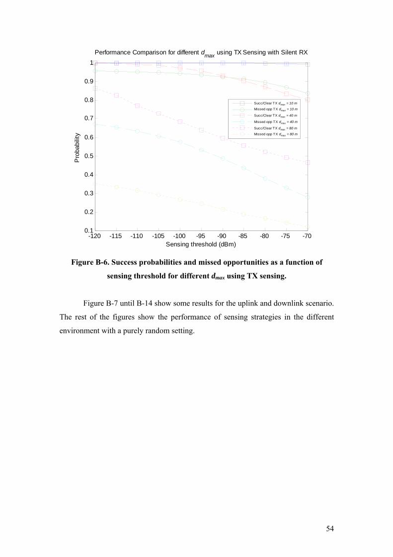
54

-120 -115 -110 -105 -100 -95 -90 -85 -80 -75 -700.1

0.2

0.3

0.4

0.5

0.6

0.7

0.8

0.9

1


Pro

babi

lity

Performance Comparison for different dmax using TX Sensing with Silent RX

Succ/Clear TX dmax = 10 m

Missed opp TX dmax = 10 m





Figure B-6. Success probabilities and missed opportunities as a function of

sensing threshold for different dmax using TX sensing.

Figure B-7 until B-14 show some results for the uplink and downlink scenario.

The rest of the figures show the performance of sensing strategies in the different

environment with a purely random setting.

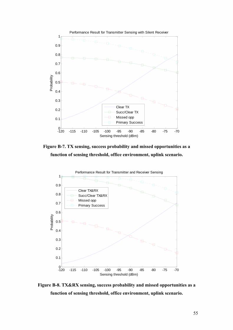
55

-120 -115 -110 -105 -100 -95 -90 -85 -80 -75 -700

0.1

0.2

0.3

0.4

0.5

0.6

0.7

0.8

0.9

1


Pro

babi

lity

Performance Result for Transmitter Sensing with Silent Receiver

Clear TXSucc/Clear TXMissed oppPrimary Success


function of sensing threshold, office environment, uplink scenario.

-120 -115 -110 -105 -100 -95 -90 -85 -80 -75 -700

0.1

0.2

0.3

0.4

0.5

0.6

0.7

0.8

0.9

1


Pro

babi

lity

Performance Result for Transmitter and Receiver Sensing

Clear TX&RXSucc/Clear TX&RXMissed oppPrimary Success


function of sensing threshold, office environment, uplink scenario.

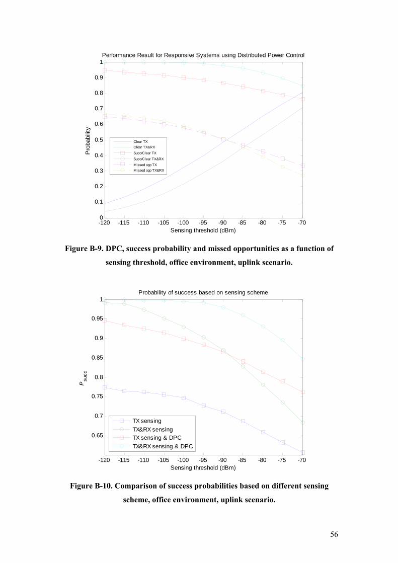
56

-120 -115 -110 -105 -100 -95 -90 -85 -80 -75 -700

0.1

0.2

0.3

0.4

0.5

0.6

0.7

0.8

0.9

1


Pro

babi

lity

Performance Result for Responsive Systems using Distributed Power Control

Clear TXClear TX&RXSucc/Clear TXSucc/Clear TX&RXMissed opp TXMissed opp TX&RX


sensing threshold, office environment, uplink scenario.

-120 -115 -110 -105 -100 -95 -90 -85 -80 -75 -70

0.65

0.7

0.75

0.8

0.85

0.9

0.95

1


Psu

cc

Probability of success based on sensing scheme



scheme, office environment, uplink scenario.

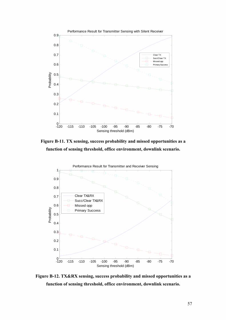
57

-120 -115 -110 -105 -100 -95 -90 -85 -80 -75 -700

0.1

0.2

0.3

0.4

0.5

0.6

0.7

0.8

0.9


Pro

babi

lity

Performance Result for Transmitter Sensing with Silent Receiver

Clear TXSucc/Clear TXMissed oppPrimary Success


function of sensing threshold, office environment, downlink scenario.

-120 -115 -110 -105 -100 -95 -90 -85 -80 -75 -700

0.1

0.2

0.3

0.4

0.5

0.6

0.7

0.8

0.9

1


Pro

babi

lity

Performance Result for Transmitter and Receiver Sensing

Clear TX&RXSucc/Clear TX&RXMissed oppPrimary Success


function of sensing threshold, office environment, downlink scenario.

58

-120 -115 -110 -105 -100 -95 -90 -85 -80 -75 -700

0.1

0.2

0.3

0.4

0.5

0.6

0.7

0.8

0.9

1


Pro

babi

lity

Performance Result for Responsive Systems using Distributed Power Control



sensing threshold, office environment, downlink scenario.

-120 -115 -110 -105 -100 -95 -90 -85 -80 -75 -70

0.4

0.5

0.6

0.7

0.8

0.9

1


Psu

cc




scheme, office environment, downlink scenario.

59

-120 -115 -110 -105 -100 -95 -90 -85 -80 -75 -700

0.1

0.2

0.3

0.4

0.5

0.6

0.7

0.8

0.9

1


Pro

babi

lity

Clear TX&RXClear TXSucc/Clear TX&RXSucc/Clear TXPrimary Success TX&RXPrimary Success TX


compared with TX sensing, office environment.

-120 -115 -110 -105 -100 -95 -90 -85 -80 -75 -700

0.1

0.2

0.3

0.4

0.5

0.6

0.7

0.8

0.9

1


Pro

babi

lity

Clear TX&RXSucc/Clear TX&RXSucc/Clear TX&RX&PCMissed oppMissed opp PCPrimary SuccessPrimary Success PC


function of sensing threshold (k = 10 dB), office environment.

60

-120 -115 -110 -105 -100 -95 -90 -85 -80 -75 -700

0.1

0.2

0.3

0.4

0.5

0.6

0.7

0.8


Pro

babi

lity



sensing threshold, office environment.

-120 -115 -110 -105 -100 -95 -90 -85 -80 -75 -700.1

0.2

0.3

0.4

0.5

0.6

0.7

0.8


Psu

cc




strategy, office environment.

61

-120 -115 -110 -105 -100 -95 -90 -85 -80 -75 -700

0.1

0.2

0.3

0.4

0.5

0.6

0.7

0.8

0.9

1


Pro

babi

lity



function of sensing threshold (k = 10 dB), commercial environment.

-120 -115 -110 -105 -100 -95 -90 -85 -80 -75 -700

0.1

0.2

0.3

0.4

0.5

0.6

0.7

0.8

0.9

1


Pro

babi

lity



function of sensing threshold (k = 10 dB), commercial environment.

62

-120 -115 -110 -105 -100 -95 -90 -85 -80 -75 -700

0.1

0.2

0.3

0.4

0.5

0.6

0.7

0.8


Pro

babi

lity



sensing threshold, commercial environment.

-120 -115 -110 -105 -100 -95 -90 -85 -80 -75 -700.1

0.2

0.3

0.4

0.5

0.6

0.7

0.8


Psu

cc




strategy, commercial environment.

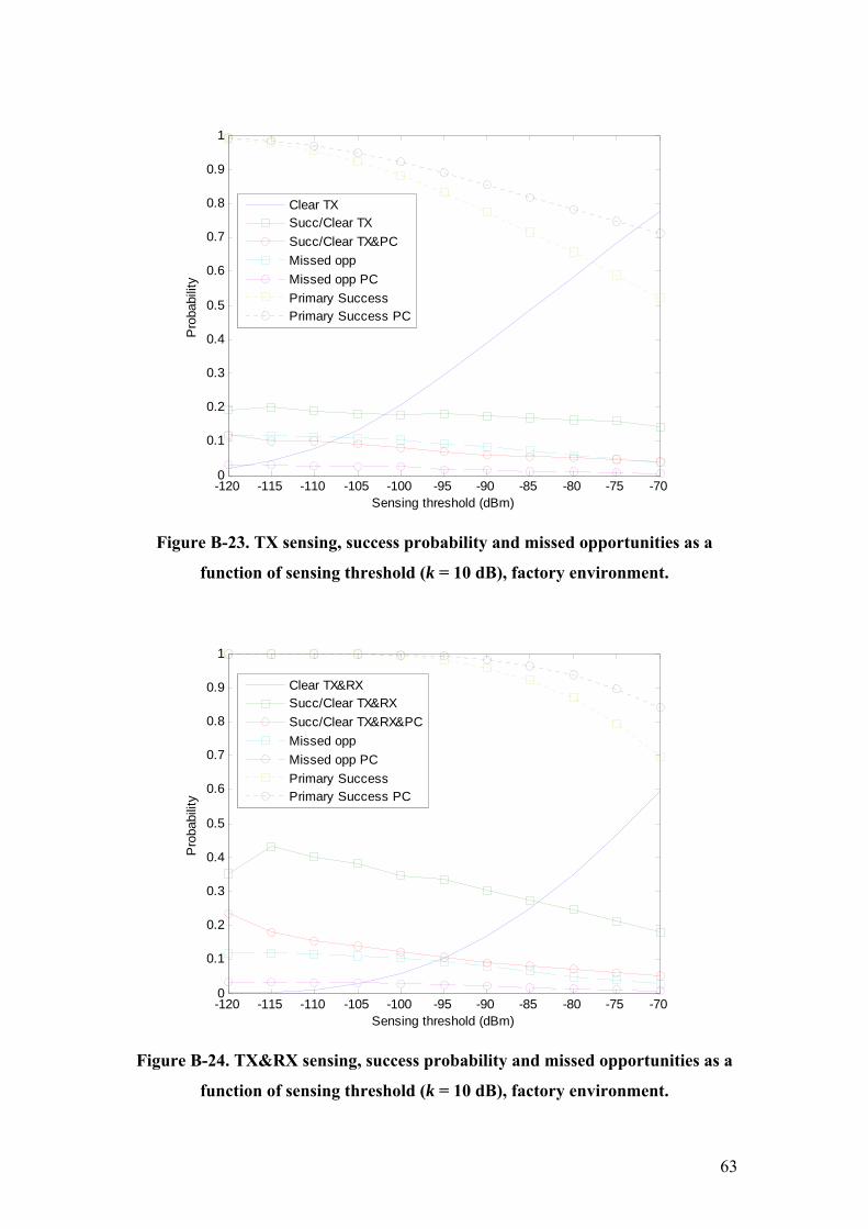
63

-120 -115 -110 -105 -100 -95 -90 -85 -80 -75 -700

0.1

0.2

0.3

0.4

0.5

0.6

0.7

0.8

0.9

1


Pro

babi

lity



function of sensing threshold (k = 10 dB), factory environment.

-120 -115 -110 -105 -100 -95 -90 -85 -80 -75 -700

0.1

0.2

0.3

0.4

0.5

0.6

0.7

0.8

0.9

1


Pro

babi

lity



function of sensing threshold (k = 10 dB), factory environment.

64

-120 -115 -110 -105 -100 -95 -90 -85 -80 -75 -700

0.1

0.2

0.3

0.4

0.5

0.6

0.7

0.8

0.9


Pro

babi

lity



sensing threshold, factory environment.

-120 -115 -110 -105 -100 -95 -90 -85 -80 -75 -700.1

0.2

0.3

0.4

0.5

0.6

0.7

0.8

0.9


Psu

cc




strategy, factory environment.

Documents

Cognitive Radio - Quantifying Reuse Opportunities in ...Cognitive Radio - Quantifying Reuse Opportunities in Indoor ... Spectrum Sensing, Spectrum Sharing. iii ... Comparison of success