Embed Size (px)
Citation preview

Saarland UniversityFaculty of Mathematics and Computer Science
Department of Computer Science
Master Thesis
Cognitive Framework for Channel Equalization inVehicular Communication Systems
Submitted byPRAHARSHA SIRSI
in May 2017
SupervisorPROF. DR.-ING. THORSTEN HERFET
AdviserM.SC. KELVIN CHELLI
ReviewersPROF. DR.-ING. THORSTEN HERFETPROF. DR.-ING. MICHAEL MÖLLER

© 2017 Telecommunications Lab, Saarland University.

Master Thesis
Praharsha Sirsi2557724
Cognitive Framework for Channel Equalization inVehicular Communication Systems
High mobility is an important characteristic in Wireless Access in VehicularEnvironments (WAVE). It results in a Doppler shift that degrades theperformance of an OFDM based receiver. This thesis focuses on variousestimation and equalization techniques that aim to compensate the effectsof high mobility. In addition to this, it introduces a cognitive frameworkthat should choose an appropriate channel estimation scheme based onchannel conditions.The IEEE 802.11p standard specifies wireless access in vehicles. It is aclose adaptation of the well known IEEE 802.11a standard. The proposedmodifications in the IEEE 802.11p standard make it more robust tomultipath propagation while at the same time making it more sensitive toDoppler shift. Thus schemes to estimate and compensate the effects ofhigh mobility pose an interesting research problem.
In particular the thesis includes the following tasks:
• Study the effects of a Doubly selective channel.
• Implement the Matching Pursuit algorithm for the IEEE 802.11pstandard.
• Develop a cognitive framework that is able to detect channel condi-tions and adapt the channel estimation and equalization schemes.
• Evaluate the performance of the developed schemes in terms of BitError Rate (BER) and complexity for different channel conditions.
Advisor:
Kelvin Chelli, M.Sc.
Supervisor:
Prof. Dr.-Ing. Thorsten Herfet
Telecommunications Lab
Department of
Computer Science
Prof. Dr.-Ing. Thorsten Herfet
Universitat des Saarlandes
Campus Saarbrucken
C6.3, 10. OG
66123 Saarbrucken
Phone: +49 681 302-70852
Fax: +49 681 302-70857
www.nt.uni-saarland.de


DECLARATION
Statement in Lieu of an OathI hereby confirm that I have written this thesis on my own and that I have not used any other media ormaterials than the ones referred to in this thesis.
Declaration of ConsentI agree to make both versions of my thesis (with a passing grade) accessible to the public by havingthem added to the library of the Computer Science Department.
Praharsha SirsiSaarbrücken, May 2017


ACKNOWLEDGEMENTS
prAy, pr(yymAdtt -vg Zq ttmAdr,
Recognition by men of noble character perhaps instillsbelief in one’s own qualities
-Kalidasa
A deep gratitude to Prof. Dr.-Ing. Thorsten Herfet for giving me an opportunity to develop thismaster’s thesis at his chair, the Telecommunications Lab. Without his unwavering support and crucialinsights, publishing the research contained in this thesis would have been impossible. The enthusiasmhe effortlessly carries, even into his lectures, has been a constant source of motivation for me from thetime I started my journey as a master’s student, and for this I am forever grateful.
The journey undertaken to complete this thesis has involved many ups and downs, but the perpetualencouragement from my adviser, Kelvin Chelli, has transformed this thesis from being merely aconclusion of my master’s study to being a window of opportunity for the future. I am profoundlythankful to him for being an inspiration and a catalyst to strive far beyond prejudiced limitations. Evenat times when the challenges seemed insurmountable, his advice and guidance has imbued calmnessfor whittling away the barriers.
I am extremely grateful to Prof. Dr.-Ing. Michael Möller for accommodating the review of mythesis in his busy schedule. I would also like to thank all members of the Telecommunication Lab forproviding insightful feedback and assistance at critical junctures. The steadfast foundations laid downby my parents and my sister is a perennial source of happiness for which any amount of gratitude isinsufficient. The sacrifices made by my soulmate, Indu, and my family, to let me follow my dreamshas been my cornerstone of strength even under the most difficult of situations and therefore thisthesis is equally theirs to cherish. I thank all my friends, specifically Sukumar and Adithya, who havecontinually advised and aided in having a life outside my studies.


ABSTRACT
Doubly selective channels or time-varying multipath channels occur when communication systemsare expected to work in a highly mobile environment. The estimation and the subsequent equalizationof such channels is a non-trivial task. Thus, an estimation scheme that is robust, precise and workswith a complexity that is applicable for consumer applications is vital to overcome the effects of sucha channel at the receiver. A novel method that implicitly estimates the Doppler shift, called as theRake Matching Pursuit, is introduced. The results show immense enhancement in estimating a doublyselective channel.
Furthermore, a novel low-complexity scheme is presented, called as Gradient Rake MatchingPursuit that optimizes the search related to the multipath delays resulting in a complexity that issignificantly lower than most Compressed Sensing based channel estimation schemes. The resultsconfirm that the performance of this modified scheme is comparable to that of the more complexRake Matching Pursuit algorithm. The dictionary is an imperative requirement of compressed sensingbased schemes and plays a decisive role in the quality of the channel estimate. In this thesis, anappropriate dictionary for the estimation is employed to produce an accurate estimate of the multipathdelays under different channel conditions. Often in literature, details regarding the generation of thedictionary and its complexity is ignored and instead a suitable dictionary is assumed to be availableat the receiver. This thesis investigates the complexity and storage demands associated with thedictionary and presents a novel scheme to build it using the concept of wavelets.
One of the most arduous challenges in Vehicular Communication Systems is a robust channelestimation scheme that performs well in stationary as well as dynamic environments. Channelestimation schemes using matching pursuit algorithms have been proven to be better than traditionalschemes in high mobility environments, but at the cost of bigger computational complexity. However,under low mobility environments, the matching pursuit algorithms, with all its greed, need not sin asoften. A cognitive framework is therefore presented to understand the channel and switch betweendifferent schemes to adequately meet various requirements. The cognitive framework optimizesthe estimation scheme based on the channel conditions and certain measurements from the receiverchain. The result is a channel estimation scheme that is robust, precise and reliable in all channelconditions while adapting the complexity to be optimal for the channel being estimated. Although,all the methods are implemented and evaluated for the IEEE 802.11p physical layer standard, theyare still applicable to any Orthogonal Frequency Division Multiplexing based wireless system that isexpected to work in highly mobile environments.


TABLE OF CONTENTS
List of figures xv
List of tables xvi
Listings xvi
Abbreviations xvii
Notations xxi
I The Prologue 1
1 Introduction 3
1.1 Motivation . . . . . . . . . . . . . . . . . . . . . . . . . . . . . . . . . . . . . 51.2 Related Research . . . . . . . . . . . . . . . . . . . . . . . . . . . . . . . . . . 6
1.2.1 Channel Estimation . . . . . . . . . . . . . . . . . . . . . . . . . . . . 71.2.2 Channel Equalization . . . . . . . . . . . . . . . . . . . . . . . . . . . 91.2.3 Cognitive Framework . . . . . . . . . . . . . . . . . . . . . . . . . . . 91.2.4 Simulation Platform . . . . . . . . . . . . . . . . . . . . . . . . . . . . 10
1.3 Outline . . . . . . . . . . . . . . . . . . . . . . . . . . . . . . . . . . . . . . . 12
II The Exposition 13
2 Foundations 15
2.1 Orthogonal Frequency Division Multiplexing . . . . . . . . . . . . . . . . . . 152.2 IEEE 802.11P . . . . . . . . . . . . . . . . . . . . . . . . . . . . . . . . . . . . 17
2.2.1 Short Training Sequence . . . . . . . . . . . . . . . . . . . . . . . . . . 192.2.2 Long Training Sequence . . . . . . . . . . . . . . . . . . . . . . . . . . 202.2.3 Pilots . . . . . . . . . . . . . . . . . . . . . . . . . . . . . . . . . . . . 202.2.4 Guard Interval . . . . . . . . . . . . . . . . . . . . . . . . . . . . . . . 222.2.5 Guard Band . . . . . . . . . . . . . . . . . . . . . . . . . . . . . . . . . 22
xii Table of contents
2.2.6 Signal Field . . . . . . . . . . . . . . . . . . . . . . . . . . . . . . . . . 222.2.7 Data Field . . . . . . . . . . . . . . . . . . . . . . . . . . . . . . . . . 23
2.3 Channels . . . . . . . . . . . . . . . . . . . . . . . . . . . . . . . . . . . . . . 252.3.1 Additive White Gaussian Noise Channel . . . . . . . . . . . . . . . . . 262.3.2 Time Selective . . . . . . . . . . . . . . . . . . . . . . . . . . . . . . . 262.3.3 Frequency Selective . . . . . . . . . . . . . . . . . . . . . . . . . . . . 272.3.4 Doubly Selective . . . . . . . . . . . . . . . . . . . . . . . . . . . . . . 282.3.5 ITU-Radio Communication Channel Models . . . . . . . . . . . . . . . 282.3.6 COST Channel Models . . . . . . . . . . . . . . . . . . . . . . . . . . 292.3.7 GSM/EDGE Channel Models . . . . . . . . . . . . . . . . . . . . . . . 30
2.4 MATLAB . . . . . . . . . . . . . . . . . . . . . . . . . . . . . . . . . . . . . . 312.5 GNU Radio . . . . . . . . . . . . . . . . . . . . . . . . . . . . . . . . . . . . . 31
2.5.1 IEEE 802.11p Model . . . . . . . . . . . . . . . . . . . . . . . . . . . . 322.6 Complexity . . . . . . . . . . . . . . . . . . . . . . . . . . . . . . . . . . . . . 362.7 Compressed Sensing . . . . . . . . . . . . . . . . . . . . . . . . . . . . . . . . 362.8 Channel Estimation . . . . . . . . . . . . . . . . . . . . . . . . . . . . . . . . 38
2.8.1 Least Squares . . . . . . . . . . . . . . . . . . . . . . . . . . . . . . . . 382.8.2 Basic Matching Pursuit . . . . . . . . . . . . . . . . . . . . . . . . . . 392.8.3 Orthogonal Matching Pursuit . . . . . . . . . . . . . . . . . . . . . . . 422.8.4 Alternate Matching Pursuit Algorithms . . . . . . . . . . . . . . . . . 45
2.9 Channel Equalization . . . . . . . . . . . . . . . . . . . . . . . . . . . . . . . 472.9.1 One-Tap Equalizer . . . . . . . . . . . . . . . . . . . . . . . . . . . . . 472.9.2 Linear Minimum Mean Square Error Equalizer . . . . . . . . . . . . . 482.9.3 Alternate Channel Equalization Methods . . . . . . . . . . . . . . . . 49
III The Plot 51
3 Methodology 53
3.1 GNU Radio Utilization . . . . . . . . . . . . . . . . . . . . . . . . . . . . . . . 533.1.1 Dynamic Channel Model . . . . . . . . . . . . . . . . . . . . . . . . . 533.1.2 Addition of Custom Blocks . . . . . . . . . . . . . . . . . . . . . . . . 55
3.2 MATLAB Simulation Platform . . . . . . . . . . . . . . . . . . . . . . . . . . 563.3 Delay Dictionary . . . . . . . . . . . . . . . . . . . . . . . . . . . . . . . . . . 57
3.3.1 The Classical Procedure . . . . . . . . . . . . . . . . . . . . . . . . . . 573.3.2 The Wavelet Procedure . . . . . . . . . . . . . . . . . . . . . . . . . . 59
3.4 Doppler Dictionary . . . . . . . . . . . . . . . . . . . . . . . . . . . . . . . . . 613.4.1 The Classical Procedure . . . . . . . . . . . . . . . . . . . . . . . . . . 613.4.2 The Wavelet Procedure . . . . . . . . . . . . . . . . . . . . . . . . . . 62

Table of contents xiii
3.5 Matching Pursuit . . . . . . . . . . . . . . . . . . . . . . . . . . . . . . . . . . 633.5.1 The Classical Matching Pursuit . . . . . . . . . . . . . . . . . . . . . . 633.5.2 Modifying the Received Vector . . . . . . . . . . . . . . . . . . . . . . 633.5.3 Tweaking the Doppler Matching Pursuit . . . . . . . . . . . . . . . . . 643.5.4 Rake Matching Pursuit . . . . . . . . . . . . . . . . . . . . . . . . . . 663.5.5 Gradient Rake Matching Pursuit . . . . . . . . . . . . . . . . . . . . . 69
3.6 The Cognitive Framework . . . . . . . . . . . . . . . . . . . . . . . . . . . . . 723.6.1 Correlation Technique . . . . . . . . . . . . . . . . . . . . . . . . . . . 733.6.2 Complex Coefficient Technique . . . . . . . . . . . . . . . . . . . . . . 76
IV The Climax 79
4 Results 81
4.1 GNU Radio Test Bed . . . . . . . . . . . . . . . . . . . . . . . . . . . . . . . 814.1.1 Dynamic Channel Model Evaluation . . . . . . . . . . . . . . . . . . . 824.1.2 BMP Delay Search Results . . . . . . . . . . . . . . . . . . . . . . . . 864.1.3 RMP Results . . . . . . . . . . . . . . . . . . . . . . . . . . . . . . . . 88
4.2 Tracking the Channel Transfer Function . . . . . . . . . . . . . . . . . . . . . 904.3 Tracking the Complex Coefficients . . . . . . . . . . . . . . . . . . . . . . . . 934.4 RMP Performance . . . . . . . . . . . . . . . . . . . . . . . . . . . . . . . . . 954.5 GRMP Performance . . . . . . . . . . . . . . . . . . . . . . . . . . . . . . . . 974.6 Correlation Based Cognitive Framework Performance . . . . . . . . . . . . . . 994.7 Complex Coefficient Based Cognitive Framework Performance . . . . . . . . . 103
V The Resolution 107
5 Conclusion 109
5.1 Contributions . . . . . . . . . . . . . . . . . . . . . . . . . . . . . . . . . . . . 1095.2 Future Work . . . . . . . . . . . . . . . . . . . . . . . . . . . . . . . . . . . . 110
References 113
Appendix A Programming Intricacies 125
A.1 Eigen Library . . . . . . . . . . . . . . . . . . . . . . . . . . . . . . . . . . . . 125A.2 VOLK . . . . . . . . . . . . . . . . . . . . . . . . . . . . . . . . . . . . . . . . 125A.3 Creating a Custom Block in GNU Radio . . . . . . . . . . . . . . . . . . . . . 125A.4 MATLAB IEEE 802.11p Simulation Platform . . . . . . . . . . . . . . . . . . 126A.5 Least Squares Fit for Tanimoto Coefficient . . . . . . . . . . . . . . . . . . . . 127

xiv Table of contents
Appendix B Mathematical Details 129
B.1 Linear Least Squares Regression . . . . . . . . . . . . . . . . . . . . . . . . . 129B.2 Ridge Regression . . . . . . . . . . . . . . . . . . . . . . . . . . . . . . . . . . 129

LIST OF FIGURES
1.1 A Vehicular Communication System . . . . . . . . . . . . . . . . . . . . . . . 32.1 An OFDM Signal . . . . . . . . . . . . . . . . . . . . . . . . . . . . . . . . . . 162.2 IEEE 802.11p Spectrum . . . . . . . . . . . . . . . . . . . . . . . . . . . . . . 182.3 IEEE 802.11p OFDM packet frame . . . . . . . . . . . . . . . . . . . . . . . . 182.4 PPDU Frame Format . . . . . . . . . . . . . . . . . . . . . . . . . . . . . . . 192.5 SIGNAL Field . . . . . . . . . . . . . . . . . . . . . . . . . . . . . . . . . . . 232.6 SERVICE Field . . . . . . . . . . . . . . . . . . . . . . . . . . . . . . . . . . . 242.7 Data Descrambler . . . . . . . . . . . . . . . . . . . . . . . . . . . . . . . . . 242.8 Convolutional Encoder . . . . . . . . . . . . . . . . . . . . . . . . . . . . . . . 252.9 IEEE 802.11p Software Loopback . . . . . . . . . . . . . . . . . . . . . . . . . 322.10 PHY Hierarchical Flowgraph . . . . . . . . . . . . . . . . . . . . . . . . . . . 333.1 GNU Radio Dynamic Channel Model . . . . . . . . . . . . . . . . . . . . . . 543.2 Phase Progression in Time Domain . . . . . . . . . . . . . . . . . . . . . . . . 653.3 Cognitive Framework Architecture . . . . . . . . . . . . . . . . . . . . . . . . 733.4 Correlation based Decision Metric Flowchart . . . . . . . . . . . . . . . . . . 743.5 Complex Coefficient based Decision Metric Flowchart . . . . . . . . . . . . . 784.1 Software Loopback with DCM . . . . . . . . . . . . . . . . . . . . . . . . . . . 824.2 DCM Settings for evaluation . . . . . . . . . . . . . . . . . . . . . . . . . . . 834.3 DCM Channel Response . . . . . . . . . . . . . . . . . . . . . . . . . . . . . . 854.4 DCM Settings for BMP delay search . . . . . . . . . . . . . . . . . . . . . . . 864.5 Six path delay, No Doppler BMP delay search . . . . . . . . . . . . . . . . . . 874.6 Six path delay, High Doppler BMP delay search . . . . . . . . . . . . . . . . . 884.7 GNU Radio RMP Results . . . . . . . . . . . . . . . . . . . . . . . . . . . . . 894.8 CTF: Magnitude . . . . . . . . . . . . . . . . . . . . . . . . . . . . . . . . . . 914.9 CTF: Phase . . . . . . . . . . . . . . . . . . . . . . . . . . . . . . . . . . . . . 924.10 Complex Coefficient Variation . . . . . . . . . . . . . . . . . . . . . . . . . . . 944.11 BER performance of RMP . . . . . . . . . . . . . . . . . . . . . . . . . . . . . 964.12 BER performance of GRMP . . . . . . . . . . . . . . . . . . . . . . . . . . . . 984.13 BER performance of Correlation Based Cognitive Framework . . . . . . . . . 1004.14 BER performance of x Based Cognitive Framework . . . . . . . . . . . . . . . 104

LIST OF TABLES
2.1 Spectrum allocation for WAVE/DSRC applications . . . . . . . . . . . . . . . 182.2 Comparison of IEEE 802.11a and IEEE 802.11p . . . . . . . . . . . . . . . . . 192.3 Polarity of Pilots . . . . . . . . . . . . . . . . . . . . . . . . . . . . . . . . . . 222.4 RATE Field within the SIGNAL Field . . . . . . . . . . . . . . . . . . . . . . 232.5 ITU Channel Model for Vehicular Environment . . . . . . . . . . . . . . . . . 292.6 Echo Profiles according to COST 207 . . . . . . . . . . . . . . . . . . . . . . . 292.7 COST 207 Fading Simulator Settings - Typical Urban . . . . . . . . . . . . . 302.8 GSM/EDGE Channel Model - Typical Urban 6 Taps . . . . . . . . . . . . . . 302.9 BMP Algorithm . . . . . . . . . . . . . . . . . . . . . . . . . . . . . . . . . . 413.1 GNU Radio Dynamic Channel Model Settings . . . . . . . . . . . . . . . . . . 553.2 RMP Delay Search Algorithm . . . . . . . . . . . . . . . . . . . . . . . . . . . 673.3 RMP Implicit Doppler Estimation . . . . . . . . . . . . . . . . . . . . . . . . 683.4 GRMP Delay Search . . . . . . . . . . . . . . . . . . . . . . . . . . . . . . . . 704.1 Scheme’s percentages for Correlation Cognitive Framework (lower SNR) . . . 1014.2 Scheme’s percentages for Correlation Cognitive Framework (higher SNR) . . 1024.3 Scheme’s percentages for x Cognitive Framework (lower SNR) . . . . . . . . . 1034.4 Scheme’s percentages for x Cognitive Framework (higher SNR) . . . . . . . . 105A.1 MATLAB Simulation Platform Compatibility . . . . . . . . . . . . . . . . . . 126
LISTINGS
A.1 Run Simulation Platform . . . . . . . . . . . . . . . . . . . . . . . . . . . . . 126A.2 TC Threshold . . . . . . . . . . . . . . . . . . . . . . . . . . . . . . . . . . . . 127

ABBREVIATIONS
3GPP 3rd Generation Partnership Project.4G Fourth Generation Mobile Telecommunications.5G Fifth Generation Mobile Networks.
ACERT Adaptive Cognition-Enhanced Radio Teams.ADROIT Adaptive Dynamic Radio Open-Source Intelligent Team.AGC Automatic Gain Control.AWGN Additive White Gaussian Noise.
BBC British Broadcasting Corporation.BEM Basis Expansion Model.BER Bit Error Rate.BMP Basic Matching Pursuit.BPSK Binary Phase Shift Keying.
CDMA Code Division Multiple Access.CoSaMP Compressive Sampling Matched Pursuit.COST European Cooperation in Science and Technology.CP Cyclic Prefix.CRC Cyclic Redundancy Check.CS Compressed Sensing.CSP Common Simulation Platform.CTF Channel Transfer Function.
DAB Digital Audio Broadcasting.DARPA Defense Advanced Research Projects Agency.DC Direct Current.DCM Dynamic Channel Model.DFT Discrete Fourier Transform.DSRC Dedicated Short Range Communications.

xviii Abbreviations
DVB Digital Video Broadcasting.DVB-T Digital Video Broadcasting - Terrestrial.DVB-T2 Digital Video Broadcasting - Second Generation Terrestrial.
EDGE Enhanced Data rates for GSM Evolution.ETSI European Telecommunications Standards Institute.EU European Union.
FCC Federal Communications Commission.FDM Frequency Division Multiplexing.FFT Fast Fourier Transform.FPGA Field-Programmable Gate Array.
GCC GNU Compiler Collection.GHz Gigahertz.GRC GNU Radio Companion.GRMP Gradient Rake Matching Pursuit.GSM Global System for Mobile Communications.
HIPERLAN High Performance Radio LAN.
IC Integrated Circuit.ICI Inter Carrier Interference.IDE Integrated Development Environment.IDFT Inverse Discrete Fourier Transform.IEEE Institute of Electrical and Electronics Engineers.IFFT Inverse Fast Fourier Transform.IoT Internet of Things.ISI Inter Symbol Interference.ITS Intelligent Transport Systems.ITU International Telecommunication Union.
LLSR Linear Least Squares Regression.LMMSE Linear Minimum Mean Square Error.LMS Least Mean Square.LP Linear Programming.LS Least Squares.LSQR Least Squares QR Decomposition.LTE Long-Term Evolution.

Abbreviations xix
MAC Medium Access Control Layer.MIP Mutual Incoherence Property.MMSE Minimum Mean Square Error.MP Matching Pursuit.MSE Mean Square Error.
NS-3 Network Simulator-3.
OFDM Orthogonal Frequency Division Multiplexing.OMP Orthogonal Matching Pursuit.OOT Out Of Tree.OSI Open Systems Interconnection model.
PAPR Peak to Average Power Ratio.PCSI Perfect Channel State Information.PHY Physical Layer.PLCP Physical Layer Convergence Protocol.PMT Polymorphic Types.PN Pseudo Noise.PPDU Physical layer Protocol Data Unit.PSDU Physical layer Service Data Unit.
QAM Quadrature Amplitude Modulation.QPSK Quadrature Phase Shift Keying.
RF Radio Frequency.RIP Restricted Isometry Property.RMP Rake Matching Pursuit.ROMP Regularized Orthogonal Matching Pursuit.
SAMP Sparsity Adaptive Matching Pursuit.SDR Software Defined Radio.SIC Successive Interference Cancellation.SICIR Successive Interference Cancellation with Interference Reduction.SINR Signal to Interference Noise Ratio.SNR Signal to Noise Ratio.SP Subspace Pursuit.StOMP Stagewise Orthogonal Matching Pursuit.

SWIG Simplified Wrapper and Interface Generator.
TC Tanimoto Coefficient.
USRP Universal Software Radio Peripheral.
V2I Vehicle to Infrastructure.V2P Vehicle to Pedestrian.V2V Vehicle to Vehicle.
WAVE Wireless Access in Vehicular Environments.WiMAX Worldwide Interoperability for Microwave Access.WLAN Wireless Local Area Networks.WPAN Wireless Personal Area Network.
XML Extensible Markup Language.

NOTATIONS
|(·)| Absolute Value or Magnitude of a Complex Number.DDD Upper-Case bold letters/symbols represent matrices.ddd Lower-Case bold letters/symbols represent vectors.mod Modulo Operation. Hadamard product or an element-wise multiplication operator.(·) Complex Conjugate.(·)H Hermitian Transpose or Conjugate Transpose of a Matrix/Vector.(·)−1 Inverse of a Matrix.∥(·)∥2 ℓ2 Norm.C Complex Space.Z Integer Numbers.card Cardinality of a set.supp Support of a Matrix/Vector.I Imaginary part of a Complex Number/Vector.R Real part of a Complex Number/Vector. Transformation from Time Domain to Frequency Domain. Transformation from Frequency Domain to Time Domain.(·)T Transpose of a Matrix/Vector.


Viele sind hartnäckig in bezug auf deneinmal eingeschlagnen Weg, wenige inbezug auf das Ziel.
Many are stubborn in pursuit of the paththey have chosen, few in pursuit of the goal
-Friedrich Nietzsche
Part I
The Prologue
1

CHAPTER 1INTRODUCTION
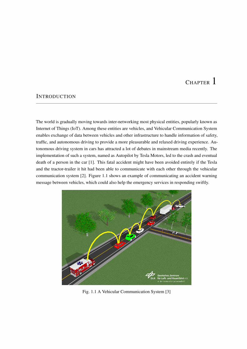
The world is gradually moving towards inter-networking most physical entities, popularly known asInternet of Things (IoT). Among these entities are vehicles, and Vehicular Communication Systemenables exchange of data between vehicles and other infrastructure to handle information of safety,traffic, and autonomous driving to provide a more pleasurable and relaxed driving experience. Au-tonomous driving system in cars has attracted a lot of debates in mainstream media recently. Theimplementation of such a system, named as Autopilot by Tesla Motors, led to the crash and eventualdeath of a person in the car [1]. This fatal accident might have been avoided entirely if the Teslaand the tractor-trailer it hit had been able to communicate with each other through the vehicularcommunication system [2]. Figure 1.1 shows an example of communicating an accident warningmessage between vehicles, which could also help the emergency services in responding swiftly.
Fig. 1.1 A Vehicular Communication System [3]

4 Introduction
The Vehicle to Pedestrian (V2P) communication system for safety encompasses a broad set of roadusers including people walking, children being pushed in strollers, people using wheelchairs or othermobility devices, passengers embarking and disembarking buses and trains, and people riding bicycles[4]. The Vehicle to Infrastructure (V2I) Communications for Safety is the wireless exchange of criticalsafety and operational data between vehicles and highway infrastructure, intended primarily to avoidmotor vehicle crashes and enable a wide range of other safety, mobility, and environmental benefits[5]. The vision for Vehicle to Vehicle (V2V) research is that each vehicle on the roadway, includingautomobiles, trucks, transit vehicles and motorcycles, will be able to communicate with other vehicles,and that this rich set of data and communications will support a new generation of active safetyapplications and systems [6]. Combining all of the above safety applications and functions requirescommunication systems that are capable of working under highly dynamic environments.
Additionally, the constant acceleration and deceleration of vehicles and its relative velocitywith respect to the elements around introduces a phenomenon called as Doppler to the wirelesscommunication signals. The signals are also affected by dense traffic conditions that increase thenoise levels and degrade the efficiency of the communication system. Moreover, excessive amount ofobjects in the environment escalates the adverse effects of multipath, and to complicate the matterfurther these objects are also in constant relative motion. Therefore, the receiver of the communicationsystem needs to utilize a channel estimation and equalization scheme that can compensate theseadverse effects. All these factors motivate the need to have a robust scheme that works reliably in allenvironments.
As a result, this thesis first looks at evaluating the traditional channel estimation methods andrevealing its limitations under high Doppler shifts. Afterwards, it investigates cutting edge channelestimation methods that are capable of reconstructing the channel at the receiver even under highDoppler shifts. Furthermore, advanced methods built upon the foundations of these methods aredeveloped and their corresponding performance is elucidated. The computational complexity of thesemethods is unveiled to be much greater when compared to the traditional methods. This motivates theneed for a framework that enables an efficient usage of these different channel estimation methodsdepending upon the channel conditions. A receiver, detecting that the channel is characterized by lowDoppler shift, need not employ a high complexity method designed for high Doppler shifts and misusevaluable resources. Contrarily, if the environment constitutes high Doppler shift, then the receivermust adopt the high complexity channel estimation method designed for such channels. The cognitiveframework introduced in this thesis is designed to switch between different channel estimationmethods depending upon the channel conditions and thereby improving the overall efficiency. Eventhough the thesis is implemented for a particular standard, the ideas presented here are applicableto any standard that utilizes Orthogonal Frequency Division Multiplexing (OFDM) in the PhysicalLayer (PHY).

1.1 Motivation 5
1.1 Motivation
A growing number of present as well as future telecommunication systems employ variants of OFDMas the transmission technology at the physical layer. OFDM is a non-trivial frequency-divisionmultiplexing scheme wherein the frequency band is split into several narrowband sub-carriers thatoverlap each other. Nevertheless, the use of harmonic functions for the sub-carriers establish anorthonormal basis that can be exploited in a transmission scenario [7]. Some of the most notableexamples of such systems range from Body- over Local- to Wide-Area Networks; from low energylow data rate sensor networks to multi-Gigabit wireless display interfaces. Despite the variety, there isa general commonality with respect to the future expectations of telecommunication systems:
• Dynamism: Mobility requirements are continuously increasing. Telecommunication systemswhere potentially both the transmitter and the receiver are in relative motion (car-2-car com-munication [8], mobile reception of terrestrial TV like Digital Video Broadcasting - SecondGeneration Terrestrial (DVB-T2) [9]) lead to requirement of coping with relative speeds of upto several 100km/h .
• High frequency: Frequencies are a scarce resource and communication systems for the futurehave to work at higher carrier frequencies of several Gigahertz (GHz) [10] up to several 10GHz[11]. Moreover, the 5th generation of wireless systems (5G) proposes a spectrum that aggregatesfrequency bands up to 86GHz [12][13].
• Sub-carrier spacing: The evolution of signal processing capabilities has led to a mass marketapplication for multicarrier systems with up to 32k carriers [14] while the channel raster hasremained unchanged. This has resulted in a continuously decreasing carrier spacing.
A trend can thus be seen where telecommunication systems have to work with higher frequencies ina highly mobile environment with an ever-increasing number of sub-carriers. Although the use ofOFDM offers several advantages, a Doppler shift caused due to mobility affects the OFDM signalby destroying the orthogonality of the narrowband sub-carriers. Thus, adjacent sub-carriers beginto interfere with each other causing Inter Carrier Interference (ICI). Moreover, the use of higherfrequencies along with a smaller sub-carrier spacing proportionally increases the effects of Dopplershifts at the receiver. Thus, a robust and low-complexity channel estimation scheme plays an importantrole in overcoming the effects of a doubly selective channel and ensuring reliable performance at theOFDM receiver.
Employing an OFDM system in the PHY is addressing a limited part of the problem. Reliablecommunication between vehicles need to compensate for the highly dynamic environment. A suiteof protocols at each layer of the Open Systems Interconnection model (OSI) need to be definedthat will facilitate not only the communication between vehicles, but also between the vehicle andother network elements. One such suite is defined by the Institute of Electrical and ElectronicsEngineers (IEEE) organization. IEEE 1609 is a family of standards for Wireless Access in Vehicular
6 Introduction
Environments (WAVE). It makes use of the IEEE 802.11p, which is a Medium Access Control Layer(MAC) and PHY specifications amendment to the IEEE 802.11 standard. Although the IEEE 802.11pis derived from the IEEE 802.11a, the latter is mainly restricted to operate in an indoor environment.
Traditional channel estimation schemes designed for the IEEE 802.11a, like the Least Squares(LS), work well under indoor environments but perform poorly under high Doppler shift environment.Matching Pursuit (MP) algorithms motivated by compressed sensing have been shown to performbetter than these traditional schemes in certain environments [15]. Compressed Sensing (CS) schemesare increasingly being used to estimate a doubly selective channel [16][17][18]. The key idea is torecover a sparse signal from very few non-adaptive, linear measurements by convex optimization [19].The wireless communication channel is inherently sparse and CS based estimation schemes exploitthis sparsity to make significant gains in complexity. Nevertheless, the computational complexity ofestimating the channel is still a bottleneck at the receiver. It is also imperative to mention that thedictionary, which is a prerequisite for CS schemes, is assumed to be available in most literature andthe complexity involved in generating the dictionary is ignored [20][21][22]. The complexity and thestorage requirements of such dictionaries needs to be investigated. Although the performance of MPis better for doubly selective channels, its higher computational burden is unnecessary under a purelyAdditive White Gaussian Noise (AWGN) channel.
To lower the complexity and the computational burden, a cognitive framework is envisioned at thereceiver that is able to switch between a low mobility channel estimation scheme (like LS) and a highmobility scheme (like MP). The incentive to develop a cognitive framework stems from the fact thatdifferent channel estimation methods do not offer reliable performance at optimum complexity underall channel conditions. For instance, the LS scheme exhibits acceptable performance only in lowmobility environments. On the other hand, the MP algorithm exhibits a significant gain in performanceunder high mobility environments but at the cost of higher complexity. Moreover, under low mobilityconditions MP performs relatively close to the LS, and thus its use in such environments is unjustified.An ideal cognitive framework that can detect the different channel conditions, and not necessarilyestimate them, at a marginal increase in complexity facilitates the switch between different channelestimation methods to consistently provide good performance at optimum complexity. Therefore,the detection of the channel characteristics, at a low computational footprint, to enable selection ofdifferent channel estimation schemes, is not a trivial problem.
1.2 Related Research
The Intelligent Transport Systems (ITS) makes use of V2V communication to allow automobiles tocommunicate with each other. The European Union (EU) had allocated the 30MHz bandwidth from5.875GHz to 5.905GHz for transport safety ITS applications in the year 2008 [23]. Although thisfrequency band is under contention [24], a lot of automotive manufacturers are actively equippingtheir cars with this system. The standard of communication for ITS in both Europe and America isbased on IEEE 802.11p as the MAC and PHY layer. The IEEE 802.11 standards suite was originally

1.2 Related Research 7
specified for Wireless Local Area Networks (WLAN) communication and there have been manyamendments to improve speed and robustness of communication. The relevant version of IEEE802.11, as of writing this report, is IEEE 802.11-2012, which incorporates "Amendment 6" that is theIEEE 802.11p-2010: Wireless Access in Vehicular Environments standard [10]. A new version of thesuite has been released [25], but there are no expected changes to the IEEE 802.11p [26].
1.2.1 Channel Estimation
The IEEE 802.11p standard uses OFDM signals in the PHY layer to transfer data from the transmitterto the receiver. The foundations of OFDM was laid down by the honored paper of Shannon [27], whereit was suggested that higher data-rate can be achieved by using a multi-carrier system. Orthogonalmultiplexing was then used to show transmission of data messages simultaneously through a linearband-limited transmission medium at a maximum data rate without inter-channel and inter-symbolinterference [28]. The capacity of such a multi-tone channel was evaluated and shown that it isfar better than a single-tone channel [29]. There are a lot of advantages of OFDM which makes itthe preferred choice for the PHY layer, and this is proven by its widespread use in most wirelessapplications [30]. However, there are a few limitations of OFDM [31] that might discourage its use incertain wireless applications.
The OFDM signals undergo adverse effects, like fading effects, when transmitted through thewireless channel. There are also certain practical impairments that are introduced, like timing offsets,in a communication system [32]. A protocol that is designed to compensate for these penalties istypically employed, and for this thesis, that protocol is the IEEE 802.11p. Synchronization is animportant and necessary step in the receiver to coarsely correct the timing and frequency offsets.Using a set of known sub-carriers to transmit information provides much better synchronization, in amulti-path environment, compared to the synchronization based only on the cyclic prefix [33]. TheIEEE 802.11 suite makes use of a particular structure, based on Pseudo-Noise sequences with goodcorrelation properties, called as Short Preamble to achieve robust synchronization [34].
The synchronization scheme achieves coarse correction of frequency and timing offsets. But forfiner correction, channel estimation schemes are employed that make use of the Long Preamble. Also,the channel might introduce inter-symbol and inter-carrier interference which need to be correctedbefore data can be decoded [35]. The method involves transmitting known data on defined sub-carriersto estimate the multiplicative channel coefficients [36]. Although the long preamble provides adefined set of values and positions in frequency domain, its position in time is also defined, and dueto Inverse Fast Fourier Transform (IFFT) being a linear function, its values in the time domain isalso defined. This enables us to employ channel estimation schemes in both domains. The LeastSquares channel estimator is a basic estimator to find the channel coefficients in frequency domain.The computational complexity involved is minimal and the performance is also overly restricted. Acomparison of different channel estimation schemes, based on performance and complexity, for IEEE802.11p, shows that schemes need some prior channel information to ensure preferable performance

8 Introduction
[37]. For example, the wiener filter proposed in [38] requires multi-path delay profile information forefficient estimation of the channel.
The MP algorithms, based on its construction and working, decomposes the signal into a linearcombination of its dictionary elements [39]. If these dictionary elements closely relate to the differentdelay paths in the multi-path environment, then the matching pursuit algorithm will find lowestdimensional linear combination of delayed versions of the transmitted symbol sequences to representthe received signal [20]. The matching pursuit algorithms are closely related to Compressed Sensing,where it is shown that one can recover sparse signals and images from fewer accurate samplescompared to the traditional methods [40]. Furthermore, there are a few other advanced channelestimation schemes for doubly selective channels that include the multidimensional Minimum MeanSquare Error (MMSE) filtering algorithms, irregular sampling techniques and the widely acceptedBasis Expansion Model (BEM) [41]. However, these schemes do not exploit the inherent sparsity ofthe channel [42][43][44] and consequently exhibit higher complexity. There are also few methodsinvolving adaptation of the pilot patterns based on the channel conditions to maximize the performanceof the system [45][46]. The disadvantages of such methods are evident as they involve modifying thecurrent standard for a marginal gain in performance, which can adversely affect other parts of thecommunication system.
The advantages in complexity and performance of the MP algorithms, when compared to otheradvanced methods, favors its use for doubly selective channels. Recently, it has been shown that theBasic Matching Pursuit (BMP) performs exceptionally well under moderate mobility environments[22]. The Orthogonal Matching Pursuit (OMP) gives a better estimate of the signal and its componentswhen the dictionary elements are not orthogonal to each other, and is also claimed to be faster andeasier to implement [47]. The idea of basis pursuit [48] was present much before the term compressedsensing [49] was coined to create an umbrella of theoretical framework. The matching pursuitalgorithms are inherently greedy [50], but there have been improvements in reducing the complexityby using a Delay-Doppler search algorithm for the DVB-T2 standard [51] and by performing anorthogonal search of multipath delays and Doppler shifts [22] for the IEEE 802.11p standard. Besides,these algorithms rely solely on a stopping criteria to provide a precise estimate of the channel using aset of linear equations. The stopping criteria measures the correlation of the estimated channel modelto the received data and is sensitive to noise and varying channel conditions. Improvements to the MPare proposed in [17] and [52] by assuming the exact sparsity in the channel which is not available inpractical systems. Thus, most CS based channel estimation algorithms either provide a marginallyinaccurate estimation of the channel due to the stopping criterion or/and have a complexity that isprohibitive for consumer applications. In this thesis, these MP algorithms are investigated and novelimprovements are proposed that offer better performance at lower complexity when compared to thetraditional methods.

1.2 Related Research 9
1.2.2 Channel Equalization
In this thesis, channel equalization is categorized as the step that absorbs the information provided bythe channel estimation schemes and rectifies the received symbols. However, there are equalizers thatassume certain channel conditions and perform equalization without channel estimation, and there area few blind equalization schemes whose performance is limited [53] in high mobility environment.The One-Tap Equalizer is a naive equalizer with a very low complexity that assumes the channelcan be completely represented by a single multiplicative complex number for each sub-carrier. Itsfavorable performance is therefore restricted to an AWGN channel that is stationary for the entireduration of the OFDM frame. The Least Mean Square (LMS) adaptive filter progressively finds thefilter coefficients using the pilot positions of the OFDM symbol [54]. Its performance is marginallybetter than the one-tap equalizer, but still limited to an AWGN channel.
The Linear Minimum Mean Square Error (LMMSE) equalizer benefits from competent channelestimation schemes. When a full channel matrix is estimated perfectly, the performance of theLMMSE equalizer for a varying channel is close to the LMS filter of AWGN channel [55]. However,the complexity of a LMMSE equalizer is higher compared to the LMS filter and One-Tap equalizer.The Successive Interference Cancellation (SIC) method for OFDM has been proven to offer admirableperformance at relatively low complexity [56]. The Successive Interference Cancellation withInterference Reduction (SICIR) decodes the signal by maximizing the Signal to Interference NoiseRatio (SINR) of each symbol. The SICIR proposed in [57] for vehicular communication follows onthe same lines as the SIC, but with a novel lower complexity method.
LSQR is a method of solving sparse linear equations and sparse least-squares problems [58],which has been used in OFDM systems in the time domain to remove ICI [59]. The LSQR methodhas an outstanding performance for relatively low complexity. If the performance can be sacrificed togain much lower complexity, then LSMR can be considered [60]. But, on the other hand, if highercomplexity is acceptable to gain much better performance to handle larger delays, then the frequencydomain LSQR algorithm can be used [61]. Nevertheless, it is imperative to note that the complexityof the channel equalizer can be drastically reduced by an accurate channel estimation scheme.
1.2.3 Cognitive Framework
The analysis of the channel estimation and channel equalization schemes enumerate the trade-offthat has to be made between the performance and complexity of the algorithms. There are manysituations, like purely AWGN channel, where there is no need to employ highly complex algorithms.But, in high mobility environment, the need to employ a complex algorithm becomes a necessity. Intheory, a metric has to determine the major characteristics of the channel and choose the right channelestimation and channel equalization scheme for that particular situation. A survey of Doppler shiftcompensation techniques is presented in [62] for vehicular networks. It exhibits that the channelestimation methods confined to the frequency domain offer poor Bit Error Rate (BER) performanceunder high mobility conditions. But exploiting the sparsity of the channel through CS schemes,

10 Introduction
such as the MP algorithm, has produced better results even for rapidly time-varying underwaterchannels [20]. Similar research for the IEEE 802.11p standard [22] demonstrates the favorableimprovement in performance under doubly selective wireless channels. But the performance gain isinsignificant under low mobility and low Signal to Noise Ratio (SNR). A mathematical frameworkwas introduced in [21] to predict the Mean Square Error (MSE) of the MP algorithm under differentchannel conditions, which showed that the MP algorithm needs the SNR to be beyond a critical pointfor accurate performance. It is evident that the MP algorithm, although compelling for high mobilityenvironments, suffers under certain channel conditions. To resolve these matters of contention, in thisthesis, the cognitive framework has been envisioned to choose the best possible channel estimationmethod that offers good performance at nominal complexity under all channel conditions.
Similar studies have been conducted in Code Division Multiple Access (CDMA) systems where,depending on the Doppler range, a feedback program selects multiple channel models and thencombines them to provide a channel estimate [63] at the cost of higher complexity. This is analogousto having a high complexity channel estimation scheme and modifying parameters of the scheme tosuit the channel under inspection. Following this approach, there are many analyses performed onmodifying certain characteristics of the existing channel estimation methods depending on the channelconditions for OFDM systems [64][65][66]. But these methods inherently have high complexityalthough they might offer better performance than the traditional methods under different channelconditions. Therefore, nearly all channel estimation methods, under different channel conditions,choose to either sacrifice performance or complexity. This forms the basis of contention that thethesis aims to solve. An appropriate framework that can switch between different channel estimationmethods can facilitate the use of the best performing method at the lowest possible complexity for allchannel conditions.
1.2.4 Simulation Platform
Defined physical layer frames conforming to the specifications of the IEEE 802.11p standard need to betransmitted through a doubly selective channel. These frames must then be forwarded to the differentchannel estimation and channel equalization blocks to understand their respective performance. Asimulation platform conforming to the specifications along-with the ability to simulate a doublyselective channel are the essential ingredients required to verify the different schemes in this thesis.In relation to this, MATLAB® simulation platform based on the MAC and PHY layer specificationsof the IEEE 802.11p has been developed and its performance has been evaluated in [67]. The PHYlayer specifications has also been flashed onto an Field-Programmable Gate Array (FPGA) and theperformance has been assessed in [68]. Similarly, a lot of research in different platforms has alreadybeen performed on the simulation of IEEE 802.11p PHY layer [69][70]. But, none of these endeavorshave led to creating a publicly available simulation platform that can be incorporated readily to testthe different schemes. However, A Simulink® model for the IEEE 802.11a exists [71] where thechannel parameters can be altered and an example performing packet error rate calculations for an

1.2 Related Research 11
end-to-end IEEE 802.11p link is also available [72]. Although they showcase that MATLAB is a validsimulation platform, editing them to integrate different channel estimation and equalization methodsis a laborious process.
Expanding the search for a versatile simulation package in other OFDM standards led to theDVB-T2 Common Simulation Platform (CSP). The DVB-T2 CSP is a software model of an end-to-end DVB-T2 chain developed collaboratively by a number of organizations within Digital VideoBroadcasting (DVB) consortium including British Broadcasting Corporation (BBC) research anddevelopment department [73]. The software is fully compliant to the DVB-T2 specification and isflexible enough to allow development and integration of custom channel estimation and equalizationfunctions. Therefore, the simulation package developed for IEEE 802.11p in this thesis emulatesthe programming philosophy of the DVB-T2 CSP. The difficulties in finding a versatile simulationpackage led to eventually reinventing the wheel, which motivated the need to make the newlydeveloped package open source. As a contribution to the research community, the simulation packageis available for download at [74] for further experimental research.
Additionally, in MATLAB, the doubly selective channel is simulated using the Rayleigh fadingchannel object which is a widely accepted model in research for wireless networks [75][76][77].Rayleigh and Rician fading channels are useful models of real-world phenomena in wireless com-munications. These phenomena include multipath scattering effects, time dispersion, and Dopplershifts that arise from relative motion between the transmitter and receiver. The channel model formultipath propagation scenarios that is implemented using the Rayleigh fading object includes discretefading paths, each with its own delay and average power gain. Default channel path modeling uses aJakes Doppler spectrum [78], with a maximum Doppler shift that can be specified. Other types ofDoppler spectra are also allowed (identical or different for all paths) which include: flat, restrictedJakes, asymmetrical Jakes, Gaussian, bi-Gaussian, and rounded [79]. A standardized channel modelusing the Rayleigh fading object can be constructed readily in MATLAB preventing the process ofreinventing the wheel for channel models. Some of the standardized channel models are EuropeanCooperation in Science and Technology (COST) 207 [80], Global System for Mobile Communica-tions (GSM) or Enhanced Data rates for GSM Evolution (EDGE) channel models [81], InternationalTelecommunication Union (ITU)-Radio Communication channel models [82], and High PerformanceRadio LAN (HIPERLAN) or HIPERLAN/2 channel models [83]. Considering all the objectivesabove, MATLAB is a valid simulation platform for the experiments performed in this thesis.
However, in addition to MATLAB and for the sake of completeness, few experiments have alsobeen conducted on another simulation platform called as GNU Radio. As already mentioned, there areother equally powerful simulation platforms that can compete with MATLAB. One of these platformsis the GNU Radio which is an open source Software Defined Radio (SDR). A SDR marks a paradigmshift towards accomplishing major part of functionality in software rather than the hardware design.A fundamental challenge of SDR is to provide the necessary computational capacity to process thewaveform applications, in particular the complex and high data rate waveform and especially forunits with strict power and size limitations [84]. The open source signal processing platform, GNU

12 Introduction
Radio, in this regard has many contributions that make it easier to rapidly prototype the designedalgorithms, test their performance and also estimate their complexity. The GNU Radio receiversupporting OFDM conforming to the IEEE 802.11a/g/p standard was developed to serve as a basis forfurther experimentation, measurements, and research on signal processing algorithms [85]. An entiretransceiver stack for IEEE 802.11p was constructed [86], tested extensively and was found to be inaccordance to the well accepted models of Network Simulator-3 (NS-3). The researchers have alsoproven that the simulations with the Universal Software Radio Peripheral (USRP) are in close relationto commercially available IEEE 802.11p devices.
1.3 Outline
The report is organized to introduce the foundations, in chapter 2, on which the thesis is going tobe based upon. The importance of OFDM is emphasized in section 2.1 which is followed by theenumeration of the different elements that make up the MAC and PHY layers of IEEE 802.11 insection 2.2. Different type of channels and their characteristics are interpreted in section 2.3 to providea glimpse into the various experiments that have to be performed to evaluate the cognitive framework.A brief introduction into the MATLAB simulation platform is presented in section 2.4. The GNURadio platform, along with the transceiver and USRP is studied in more detail in section 2.5. Insection 2.6, the process to calculate the complexity of the algorithms is introduced. Mathematicalformulations, and their respective explanation, of different channel estimation schemes is presented insection 2.8. This is closely followed by description of different equalization schemes in section 2.9 toconclude the chapter.
The next chapter, chapter 3, is concerning the methodology and implementation of the differentfacets of this thesis. At the beginning, in section 3.1, application details of the GNU Radio is fulfilledand the various settings that have to be listed to simulate the desired channel models is cataloged.This is followed by outlining the intricacies of the MATLAB simulation platform in section 3.2.Construction of the delay and Doppler dictionaries for the matching pursuit algorithms is annotated insection 3.3 and section 3.4, respectively. The core idea of the matching pursuit algorithms and theimprovements made upon them are elucidated in section 3.5. Finally, the cognitive framework and itsimplementation details are given in section 3.6.
The numerous experiments and their results are published in chapter 4. The screen-shots of theGNU Radio test bed along with the changes to the initial flow-graph is highlighted in section 4.1.Resulting plots with their respective implications are emphasized in subsection 4.1.3. The performanceof the Rake Matching Pursuit (RMP) algorithm in tracking the channel transfer function is shown insection 4.2. The BER performance of the different algorithms introduced in the thesis is displayed insection 4.4 and section 4.5. The chapter is concluded by advertising the performance of the cognitiveframeworks in section 4.6 and section 4.7. The conclusions and the scope of future work of this thesisis published in chapter 5

What we want is to see the child in pursuitof knowledge, and not knowledge in pursuitof the child.
George Bernard Shaw
Part II
The Exposition
13

CHAPTER 2FOUNDATIONS
Introduction to the concepts and theory utilized in this thesis is presented in this chapter. However,the chapter does not deal with intricate details of programming or basic communication concepts. Itmainly outlines the theory that may be unfamiliar to the reader. This chapter also contains the prefaceto the different tools and algorithms used in the thesis.
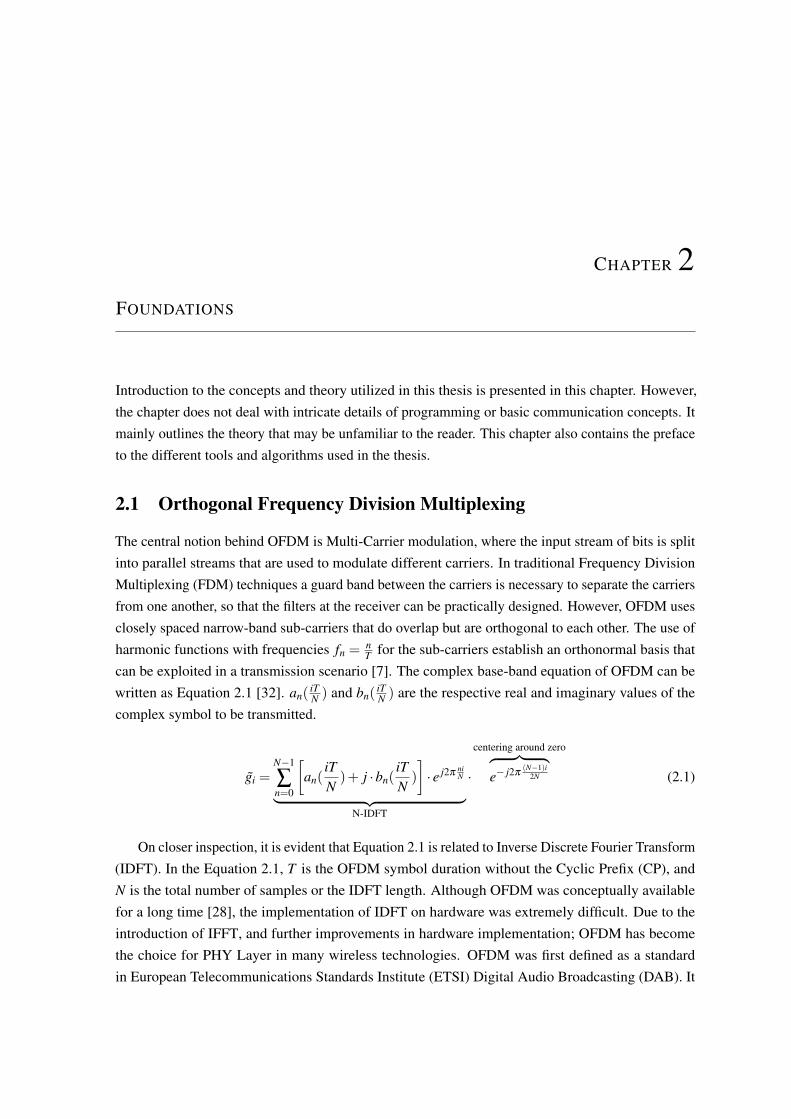
2.1 Orthogonal Frequency Division Multiplexing
The central notion behind OFDM is Multi-Carrier modulation, where the input stream of bits is splitinto parallel streams that are used to modulate different carriers. In traditional Frequency DivisionMultiplexing (FDM) techniques a guard band between the carriers is necessary to separate the carriersfrom one another, so that the filters at the receiver can be practically designed. However, OFDM usesclosely spaced narrow-band sub-carriers that do overlap but are orthogonal to each other. The use ofharmonic functions with frequencies fn =
nT for the sub-carriers establish an orthonormal basis that
can be exploited in a transmission scenario [7]. The complex base-band equation of OFDM can bewritten as Equation 2.1 [32]. an(
iTN ) and bn(
iTN ) are the respective real and imaginary values of the
complex symbol to be transmitted.
gi =N−1
∑n=0
[an(
iTN)+ j ·bn(
iTN)
]· e j2π
niN︸ ︷︷ ︸
N-IDFT
·
centering around zero︷ ︸︸ ︷e− j2π
(N−1)i2N (2.1)
On closer inspection, it is evident that Equation 2.1 is related to Inverse Discrete Fourier Transform(IDFT). In the Equation 2.1, T is the OFDM symbol duration without the Cyclic Prefix (CP), andN is the total number of samples or the IDFT length. Although OFDM was conceptually availablefor a long time [28], the implementation of IDFT on hardware was extremely difficult. Due to theintroduction of IFFT, and further improvements in hardware implementation; OFDM has becomethe choice for PHY Layer in many wireless technologies. OFDM was first defined as a standardin European Telecommunications Standards Institute (ETSI) Digital Audio Broadcasting (DAB). It

16 Foundations
was then used in the Digital Video Broadcasting - Terrestrial (DVB-T) standard. Recently, the IEEE802.11 [10] or WiFi, the IEEE 802.16 [87] or Worldwide Interoperability for Microwave Access(WiMAX) and IEEE 802.15 [88] or Wireless Personal Area Network (WPAN) define OFDM in theirstandards to achieve high data rates. The Fourth Generation Mobile Telecommunications (4G) cellulartechnology - Long-Term Evolution (LTE) [89], DVB-T2 [73] and Fifth Generation Mobile Networks(5G) [13] also use OFDM. Figure 2.1 shows an OFDM signal.
Am
plitu
de
(v)
Time (s)
Frequency (Hz)
T
Guard Interval
Fig. 2.1 An OFDM Signal [35]
The narrow-band carriers, as seen in Figure 2.1, is free of any ICI. The symbols in time domainalso have a guard interval between them to avoid Inter Symbol Interference (ISI). In a multi-pathenvironment, many copies of a symbol will be received at the receiver after undergoing differentdelays. To compensate for such an effect, systems typically make use of a CP, where defined numberof samples from the end of the data stream are added to the start of the OFDM symbol in the timedomain. OFDM also incorporates a guard band to avoid the symbol energy from spilling outside thedefined bandwidth. Few narrow-band sub-carriers at the beginning of the spectrum and towards theend of the spectrum are simply set to zero to create the guard band.
Advantages. OFDM is much more complicated compared to traditional multiplexing schemes,but it does provide definite gains, in terms of data transmission, over the traditional schemes.
• Typically, transmission specifications are severely stringent on the bandwidth and amount ofpower that can be transmitted by a system. OFDM is one of the best methods to exploit thislimited spectrum by using the narrow-band carriers.
• The input data stream in OFDM is converted to a lower bit rate parallel stream, which increasesthe symbol duration, in turn making the OFDM system more resistant to multi-path effects.

2.2 IEEE 802.11P 17
• The lower bit-rate symbols also results in lower ISI. The use of cyclic prefix in OFDMcontributes to making the entire OFDM symbol more robust against multi-path effects.
• Integrated Circuit (IC) for IFFT and Fast Fourier Transform (FFT) are fast, reliable andeconomical. This makes the OFDM implementation in a communication system exceptionallycompetitive even in the commercial market.
Disadvantages. Although there are many advantages to using an OFDM scheme, there are a fewdrawbacks that have to be taken into account before considering it as the medium of transmission.
• Carrier frequency offsets and drifts can be dangerous to an OFDM signal. The orthogonalitybetween the sub-carriers are lost due to these frequency shifts. Doppler effects results infrequency shifts, and these shifts are not a constant value for all frequencies.
• OFDM has a high Peak to Average Power Ratio (PAPR). The lower bit-rate combined with thecyclic prefix and high spectral efficiency usually means that the PAPR will be large. This putshigher demands on the amplifiers in the system.
In conclusion, OFDM offers several advantages but the major drawback is its susceptibility toDoppler shifts that destroy the orthogonality of the narrowband sub-carriers due to ICI. High mobilityin a multipath propagation environment leads to a doubly selective or a time-varying multipath channelthat deteriorates the performance of an OFDM system. Moreover, the estimation and the subsequentequalization of such a channel is a non-trivial task since the channel state is continuously changingand the equalizer must be constantly redesigned to match the channel [42][90]. Therefore, a robustchannel estimation scheme is essential to compensate for the disturbances experienced by the OFDMsignal, when passing through a doubly selective channel.
2.2 IEEE 802.11P
The IEEE 802.11p, historically, was defined as the PHY standard for WAVE and Dedicated ShortRange Communications (DSRC). Some of the frequency bands allocated for DSRC applications indifferent regions are shown in Table 2.1. The Federal Communications Commission (FCC) allocated75MHz of spectrum in the 5.9GHz band for use by ITS vehicle safety and mobility applications[91]. In this frequency band, the IEEE 802.11p created 7 different channels, each having a 10MHzbandwidth as shown in Figure 2.2. The control channel is used to transmit safety messages, and servicechannels are used for other data transmissions. It offers data exchange among vehicles and betweenvehicles and roadside infrastructure within a range of 1km while using a transmission rate of 3Mbpsto 27Mbps upto a vehicle velocity of 260km/h [92]. Although, the bit rate of the primary standard(IEEE 802.11a) was up to 54Mbps, the bit rate of IEEE 802.11p has been reduced to half because ofthe limitations of PHY layer in coping with the high mobility vehicular network characteristics [93].
The main aspects of the IEEE 802.11p under consideration in this thesis are the PHY layerspecifications. The IEEE 802.11p, as mentioned in section 1.1, is akin to the IEEE 802.11a standard

18 Foundations
Table 2.1 Spectrum allocation for WAVE/DSRC applications [92]
Country/Region Frequency Bands(MHz) Reference Documents
ITU-R (ISM band) 5725-5875 Article 5 of Radio Regula-tions
Europe 5795-5815, 5855/5875,5905/5925
ETS 202-663, ETSI EN302-571, ETSI EN 301-893
North America 902-928, 5850-5925 FCC 47 CFRJapan 715-725, 5770-5850 MIC EO Article 49
Fig. 2.2 IEEE 802.11p Spectrum [94]
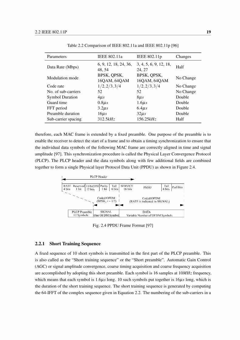
which is widely used for WiFi. The OFDM packet frame of IEEE 802.11p is shown in Figure 2.3,which is analogous to the IEEE 802.11a packet. PHY layer in IEEE 802.11p is quite similar to IEEE802.11a but with some additional features to handle the vehicular environment, so the priority changesdepending upon the situation it is implemented [95]. To overcome the difficulty in communication inWAVE, changes done in PHY layer of IEEE 802.11p compared to IEEE 802.11a is shown in Table 2.2.In vehicular environments, the maximum multi-path delay is expected to be more than the indoorenvironment. Therefore, the guard time in IEEE 802.11p is doubled. The data rate in IEEE 802.11pfor similar modulation schemes, compared to IEEE 802.11a, is halved as the bandwidth is also halved.This also has a consequence on the symbol period, which is doubled compared to IEEE 802.11a.These changes are in accordance to the requirements of the current urban vehicular environmentwhere the Doppler shifts aren’t substantial enough to adversely affect the OFDM transmission.
The beginning of a MAC frame has to be properly detected by a receiver in order to correctlyinterpret the following data symbols. The receiver needs to estimate the exact sample positions,
Fig. 2.3 IEEE 802.11p OFDM packet frame [37]
2.2 IEEE 802.11P 19
Table 2.2 Comparison of IEEE 802.11a and IEEE 802.11p [96]
Parameters IEEE 802.11a IEEE 802.11p Changes
Data Rate (Mbps)6, 9, 12, 18, 24, 36,48, 54
3, 4, 5, 6, 9, 12, 18,24, 27
Half
Modulation modeBPSK, QPSK,16QAM, 64QAM
BPSK, QPSK,16QAM, 64QAM
No Change
Code rate 1/2,2/3,3/4 1/2,2/3,3/4 No ChangeNo. of sub-carriers 52 52 No ChangeSymbol Duration 4µs 8µs DoubleGuard time 0.8µs 1.6µs DoubleFFT period 3.2µs 6.4µs DoublePreamble duration 16µs 32µs DoubleSub-carrier spacing 312.5kHz 156.25kHz Half
therefore, each MAC frame is extended by a fixed preamble. One purpose of the preamble is toenable the receiver to detect the start of a frame and to obtain a timing synchronization to ensure thatthe individual data symbols of the following MAC frame are correctly aligned in time and signalamplitude [97]. This synchronization procedure is called the Physical Layer Convergence Protocol(PLCP). The PLCP header and the data symbols along with few additional fields are combinedtogether to form a single Physical layer Protocol Data Unit (PPDU) as shown in Figure 2.4.
Fig. 2.4 PPDU Frame Format [97]
2.2.1 Short Training Sequence
A fixed sequence of 10 short symbols is transmitted in the first part of the PLCP preamble. Thisis also called as the “Short training sequence” or the “Short preamble”. Automatic Gain Control(AGC) or signal amplitude convergence, coarse timing acquisition and coarse frequency acquisitionare accomplished by adopting this short preamble. Each symbol is 16 samples at 10MHz frequency,which means that each symbol is 1.6µs long. 10 such symbols put together is 16µs long, which isthe duration of the short training sequence. The short training sequence is generated by computingthe 64-IFFT of the complex sequence given in Equation 2.2. The numbering of the sub-carriers in a

20 Foundations
64-OFDM symbol are done from −32 to +31, totaling to 64 sub-carriers. The sub-carrier labeled as“0” is called as the Direct Current (DC) sub-carrier and is always set to the value zero. It correspondsto the center frequency of the Radio Frequency (RF) signal being transmitted. But, if we consider thebase-band version of the OFDM symbol given in Equation 2.1, then this position corresponds to thezero frequency, or DC component of the OFDM symbol.
sss−26,26 =√
13/6 · (0,0,1+ j,0,0,0,−1− j,0,0,0,1+ j,0,0,
0,−1− j,0,0,0,−1− j,0,0,0,1+ j,0,0,0,
0,0,0,0,−1− j,0,0,0,−1− j,0,0,0,1+ j,
0,0,0,1+ j,0,0,0,1+ j,0,0,0,1+ j,0,0)
(2.2)
Extensive research has been conducted in utilizing the short training sequence for synchronizationin WLAN systems [98]. However, the performance and the synchronization accuracy degrades underlow SNR and is limited to an AWGN channel [99]. The investigation and subsequent evaluation of dif-ferent synchronization schemes is beyond the scope of this thesis and therefore perfect synchronizationis assumed in the MATLAB simulation platform.
2.2.2 Long Training Sequence
The “Long preamble” or “Long training sequence” in the PLCP header is used for channel estimation,finer timing offset correction and also finer frequency offset corrections. They can also be used totrack the channel variations from one OFDM frame to another, but as they are placed only at thebeginning of an OFDM frame, channel variations within the OFDM frame cannot be tracked usingthe Long Preamble. There are actually two Long preambles in the PLCP header. Each long preambleis 6.4µs long consisting of 52 non-zero sub-carriers and 12 null sub-carriers. Between the shortpreamble and the long preamble, two Guard Interval sequences that are the cyclic prefix of the longpreamble are added, where each of cyclic prefix is 1.6µs long. Therefore, the PLCP preamble consistsof one short training sequence of 16µs, two cyclic prefix sequences of 1.6µs each, and two longpreambles of 6.4µs each, accumulating to a total duration of 32µs. The long training sequence isgenerated by computing the 64-IFFT of the sequence given in Equation 2.3.
lll−26,26 =(1,1,−1,−1,1,1,−1,1,−1,1,1,1,1,
1,1,−1,−1,1,1,−1,1,−1,1,1,1,1,
0,1,−1,−1,1,1,−1,1,−1,1,−1,−1,−1,
−1,−1,1,1,−1,−1,1,−1,1,−1,1,1,1,1)
(2.3)
2.2.3 Pilots
In each of the OFDM data symbols following the PLCP header, there are 4 pilot sub-carriers thatcan be used for further channel estimation and correction. As the PLCP header is at the beginning of
2.2 IEEE 802.11P 21
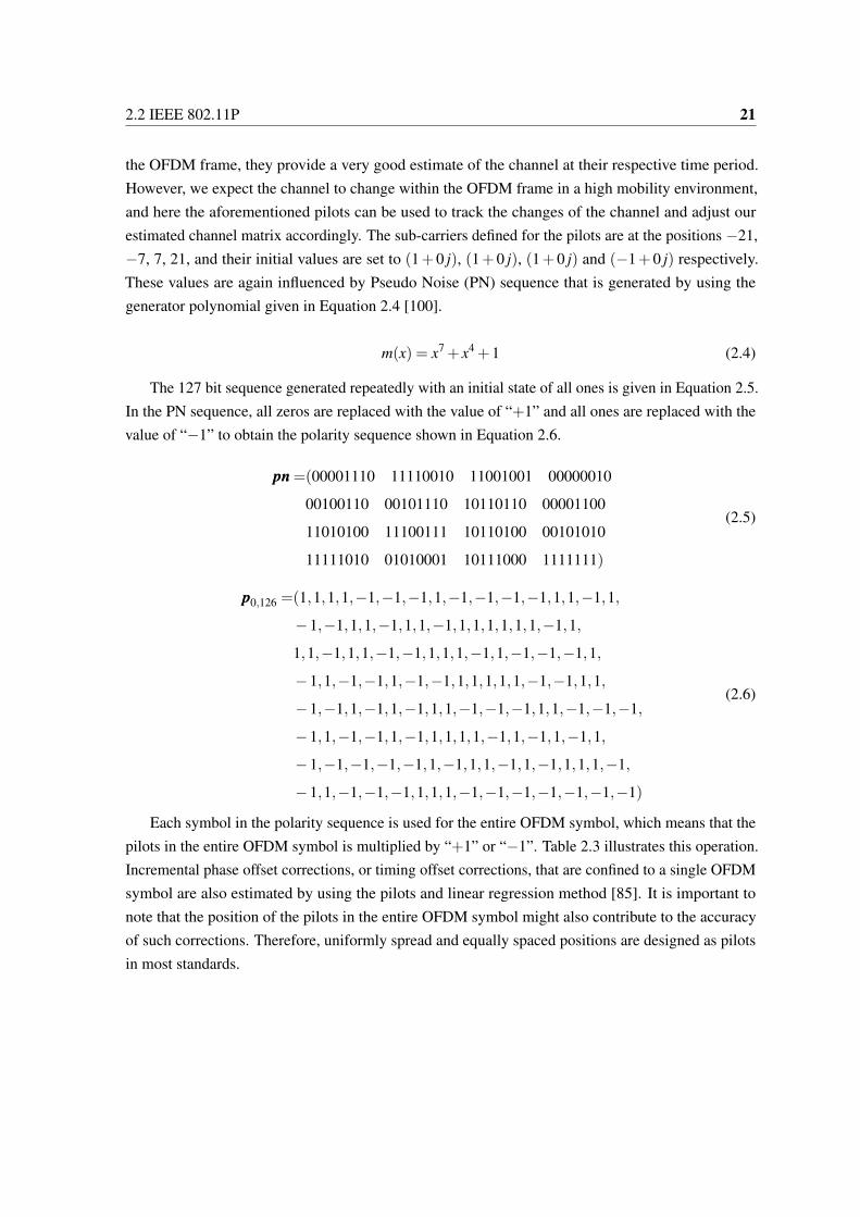
the OFDM frame, they provide a very good estimate of the channel at their respective time period.However, we expect the channel to change within the OFDM frame in a high mobility environment,and here the aforementioned pilots can be used to track the changes of the channel and adjust ourestimated channel matrix accordingly. The sub-carriers defined for the pilots are at the positions −21,−7, 7, 21, and their initial values are set to (1+0 j), (1+0 j), (1+0 j) and (−1+0 j) respectively.These values are again influenced by Pseudo Noise (PN) sequence that is generated by using thegenerator polynomial given in Equation 2.4 [100].
m(x) = x7 + x4 +1 (2.4)
The 127 bit sequence generated repeatedly with an initial state of all ones is given in Equation 2.5.In the PN sequence, all zeros are replaced with the value of “+1” and all ones are replaced with thevalue of “−1” to obtain the polarity sequence shown in Equation 2.6.
pppnnn =(00001110 11110010 11001001 00000010
00100110 00101110 10110110 00001100
11010100 11100111 10110100 00101010
11111010 01010001 10111000 1111111)
(2.5)
ppp0,126 =(1,1,1,1,−1,−1,−1,1,−1,−1,−1,−1,1,1,−1,1,
−1,−1,1,1,−1,1,1,−1,1,1,1,1,1,1,−1,1,
1,1,−1,1,1,−1,−1,1,1,1,−1,1,−1,−1,−1,1,
−1,1,−1,−1,1,−1,−1,1,1,1,1,1,−1,−1,1,1,
−1,−1,1,−1,1,−1,1,1,−1,−1,−1,1,1,−1,−1,−1,
−1,1,−1,−1,1,−1,1,1,1,1,−1,1,−1,1,−1,1,
−1,−1,−1,−1,−1,1,−1,1,1,−1,1,−1,1,1,1,−1,
−1,1,−1,−1,−1,1,1,1,−1,−1,−1,−1,−1,−1,−1)
(2.6)
Each symbol in the polarity sequence is used for the entire OFDM symbol, which means that thepilots in the entire OFDM symbol is multiplied by “+1” or “−1”. Table 2.3 illustrates this operation.Incremental phase offset corrections, or timing offset corrections, that are confined to a single OFDMsymbol are also estimated by using the pilots and linear regression method [85]. It is important tonote that the position of the pilots in the entire OFDM symbol might also contribute to the accuracyof such corrections. Therefore, uniformly spread and equally spaced positions are designed as pilotsin most standards.

22 Foundations
Table 2.3 Polarity of Pilots
OFDM Symbol # Polarity #Pilots
−21 −7 21 7
0 1 (1+0 j) (1+0 j) (1+0 j) (−1+0 j)1 1 (1+0 j) (1+0 j) (1+0 j) (−1+0 j)2 1 (1+0 j) (1+0 j) (1+0 j) (−1+0 j)3 1 (1+0 j) (1+0 j) (1+0 j) (−1+0 j)4 −1 (−1+0 j) (−1+0 j) (−1+0 j) (1+0 j)5 −1 (−1+0 j) (−1+0 j) (−1+0 j) (1+0 j)6 −1 (−1+0 j) (−1+0 j) (−1+0 j) (1+0 j)7 1 (1+0 j) (1+0 j) (1+0 j) (−1+0 j)
2.2.4 Guard Interval
The guard interval is used in OFDM to combat multi-path effects and avoid ISI. The guard intervalhere, is also called as the cyclic prefix, where a few defined number of samples from the end of theOFDM symbol is prefixed to the start of the symbol. The number of samples taken as cyclic prefix inIEEE 802.11p is defined to be 16 samples, or 25% of the entire OFDM symbol duration. This makesthe cyclic prefix 1.6µs long, having 16 samples, which is twice as long as the guard interval in IEEE802.11a. As long as the distance between the different paths of the multi-path effects stay below thelength of the cyclic prefix, the ISI can be compensated [32].
2.2.5 Guard Band
The guard band that is located at the outer limits of the frequency band is used to adhere to the strictspectral mask defined by the standardizing committees. In IEEE 802.11p the first 6 sub-carriers, andthe last 5 sub-carriers are set to zero to create the guard band, which is the same as IEEE 802.11a.Although this reduces the maximum data rate that can be achieved, it is important to avoid aliasing, sothat the adjacent channels shown in Figure 2.2 do not interfere with each other.
2.2.6 Signal Field
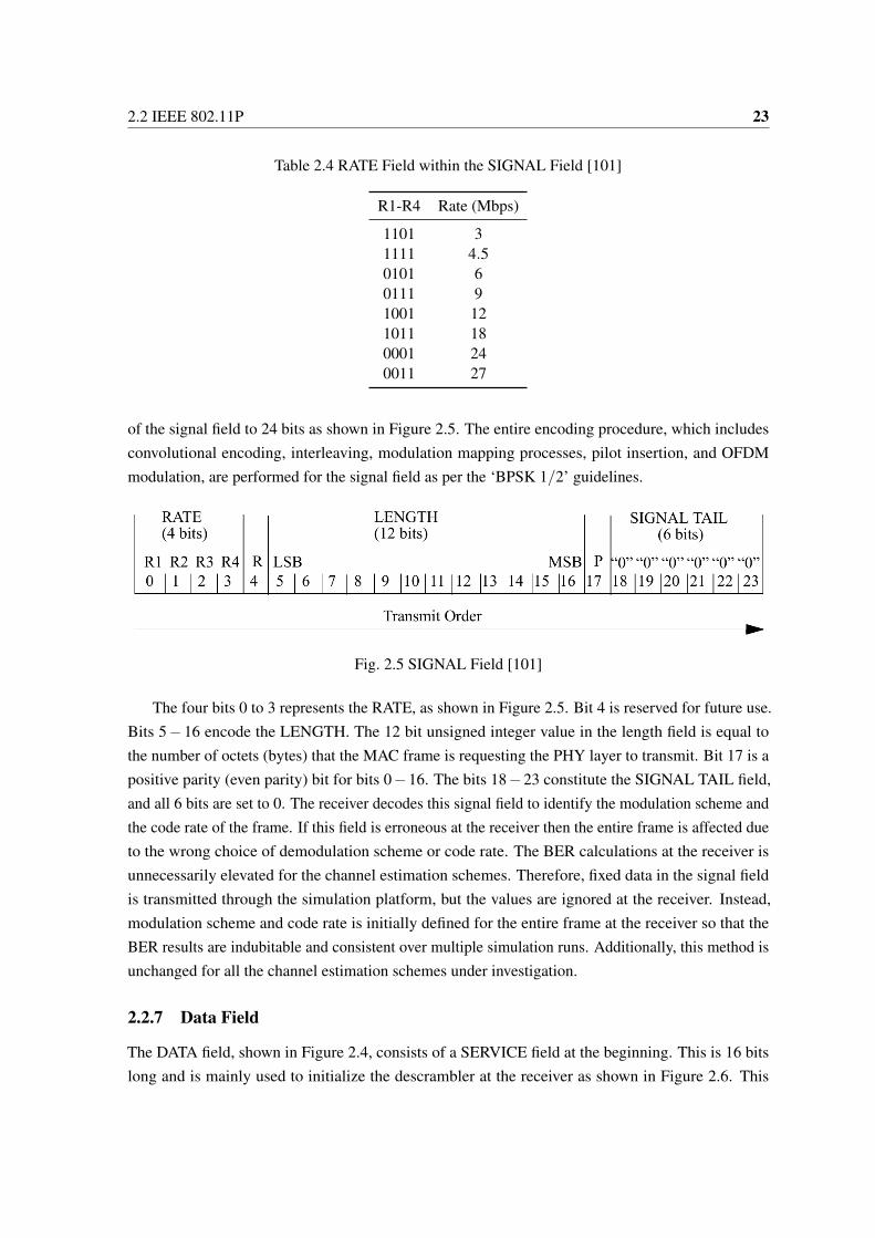
Another integral part of the PLCP header is the SIGNAL field that follows the OFDM training symbolsdescribed above. Within the signal field, the RATE field conveys the type of modulation and thecoding rate for the entire frame and its values are given in Table 2.4. This means that the modulationscheme and code rates for the data sub-carriers do not vary from one OFDM symbol to another and isconsistent for the entire frame. Additionally, the schemes are also fixed for each sub-carrier.
The LENGTH field also exists within the signal field, which is employed to transmit the size of theMAC frame [101]. The encoding is performed with Binary Phase Shift Keying (BPSK) modulationof the sub-carriers and using convolutional coding at a coding rate of 1/2, which restricts the size
2.2 IEEE 802.11P 23
Table 2.4 RATE Field within the SIGNAL Field [101]
R1-R4 Rate (Mbps)
1101 31111 4.50101 60111 91001 121011 180001 240011 27
of the signal field to 24 bits as shown in Figure 2.5. The entire encoding procedure, which includesconvolutional encoding, interleaving, modulation mapping processes, pilot insertion, and OFDMmodulation, are performed for the signal field as per the ‘BPSK 1/2’ guidelines.
Fig. 2.5 SIGNAL Field [101]
The four bits 0 to 3 represents the RATE, as shown in Figure 2.5. Bit 4 is reserved for future use.Bits 5− 16 encode the LENGTH. The 12 bit unsigned integer value in the length field is equal tothe number of octets (bytes) that the MAC frame is requesting the PHY layer to transmit. Bit 17 is apositive parity (even parity) bit for bits 0−16. The bits 18−23 constitute the SIGNAL TAIL field,and all 6 bits are set to 0. The receiver decodes this signal field to identify the modulation scheme andthe code rate of the frame. If this field is erroneous at the receiver then the entire frame is affected dueto the wrong choice of demodulation scheme or code rate. The BER calculations at the receiver isunnecessarily elevated for the channel estimation schemes. Therefore, fixed data in the signal fieldis transmitted through the simulation platform, but the values are ignored at the receiver. Instead,modulation scheme and code rate is initially defined for the entire frame at the receiver so that theBER results are indubitable and consistent over multiple simulation runs. Additionally, this method isunchanged for all the channel estimation schemes under investigation.
2.2.7 Data Field
The DATA field, shown in Figure 2.4, consists of a SERVICE field at the beginning. This is 16 bitslong and is mainly used to initialize the descrambler at the receiver as shown in Figure 2.6. This

24 Foundations
is followed by the MAC layer data symbols aggregated into the Physical layer Service Data Unit(PSDU), which contains the data that is to be transmitted over the channel. The 6 TAIL bits shown inFigure 2.4 are required to return the convolutional encoder to the zero state. Additionally, PAD bitsare vital to ensure adequate amount of bits for complete mapping onto the OFDM symbols.
Fig. 2.6 SERVICE Field [101]
The DATA field, composed of SERVICE, PSDU, tail, and pad parts, are scrambled with a length-127 frame-synchronous scrambler. The generator polynomial is the same as given in Equation 2.4.Hence, the sequence generated is also identical to Equation 2.5. The data descrambler is illustrated inFigure 2.7.
Fig. 2.7 Data Descrambler [101]
The entire DATA field is also encoded using the convolutional coder with the generator polynomi-als g0 = 1338 and g1 = 1718. Combining this with specific puncturing patterns results in differentcode rates. The convolutional coder is illustrated in Figure 2.8 for a constraint length of k = 7.
After convolutional encoding and puncturing, interleaving of the data is performed at the trans-mitter. Generally the errors due to noise in wireless channels are burst errors, which means thata lot of errors occur within a small amount of time [32]. To circumvent this effect, interleavingis implemented that pseudo randomly distributes portions of the data over the entire stream [101].Combining this with convolutional encoding, which can also compensate for burst errors, ensuresconsiderable reduction in the BER. The modifications to the data field, which are essential for anend-to-end communication system, have substantial positive contributions towards the performance ofthe channel estimation schemes. The SERVICE field, which is used to initialize the descrambler, canbe considered as additional data that is being transmitted and is indeed inconsequential to the channelestimation scheme. The scrambler is utilized to randomize data, such that a lengthy stream of “1’s” or“0’s” don’t occur contiguously. The descrambler performs the inverse process. These methods also

2.3 Channels 25
Fig. 2.8 Convolutional Encoder [101]
contribute in reduction of BER which could distort the genuine performance of the channel estimationschemes in the simulation platform.
Furthermore, the effect of convolutional coding and interleaving are significant enough to deceivethe researcher into believing that the gain in performance might be due to the developments in thechannel estimation scheme. Attributing the performance to the channel estimation and equalizationschemes alone becomes problematic and inaccurate. To avoid such points of contention and representthe legitimate performance of the various channel estimation schemes, all modifications to thedata field are ignored in the simulation platform. Therefore, a block of unmodified data prefixedwith the PLCP header is transformed into OFDM symbols, as per the guidelines introduced before,and transmitted through the channel. At the receiver, the received data, after channel estimationand channel equalization, is compared with the template that is transmitted to calculate the BERperformance. This method ensures that the measured performance is a sincere characteristic of thechannel estimation scheme and is consistent over several iterations. Additionally, it is encouragingto note that, all the above methods used for modifying data can only improve the BER performancerather than degrade it.
2.3 Channels
In communications, a channel refers to the physical medium that forms the connection between thetransmitter and receiver. For IEEE 802.11p, we make use of microwaves in the 5GHz domain toform the connection between the transmitter and receiver in the wireless medium. There are manyphysical phenomena, like reflection, refraction, and diffraction, that affects the signal passing throughthe wireless medium. However, there are many other effects in the wireless medium, like fading, thatare best modeled mathematically or statistically. Generally, the actual channels in the environmentare too complex to be modeled perfectly, hence we make use of statistical channels that have beendeveloped on real world measurements. These channel models have been tested extensively and areaccepted in the community as the standard models on which simulations can be performed.

26 Foundations
2.3.1 Additive White Gaussian Noise Channel
The AWGN channel model is one of the most common channel which assumes that the noise isadditive, has a very large bandwidth and is a superposition of many independent sources [35]. In thischannel model, it is assumed that there are no multi-path or Doppler effects. It only assumes that thereis additive noise that has a probability density function same as the Gaussian distribution given inEquation 2.7. z is a random variable representing the noise amplitude, p(z) represents the probabilityof the random variable, and σ2 represents the variance of the Gaussian distribution.
p(z) =1√
2πσ2exp(−z2
2σ2
)(2.7)
However, there is a delay when the signal passes through the AWGN channel, which is the pathdelay between the transmitter and the receiver. This is nothing but a timing offset that is easilycorrected by the synchronization block in the receiver. The variations in noise amplitude, as it isassumed to be independent and identically distributed, are only scalars for each sample. The LSestimator is extremely efficient for such a channel, as the channel is also assumed to be stationaryfor the entire OFDM frame. The received symbols yi are the sum of the transmitted symbols xi andthe noise symbols zi, where zi has values that are drawn from a Gaussian distribution, as shown inEquation 2.8.
yi = xi + zi (2.8)
Evaluating the performance of the channel estimation and equalization schemes for a purelyAWGN channel is unproductive in this thesis, as the LS scheme has already been established tocompensate such channels entirely [37]. The major focus of this thesis is evaluating the performanceof the schemes under much more complex channels.
2.3.2 Time Selective
A general channel model is represented in Equation 2.9 [32]. It shows that the received symbols y(t)is the convolution of the time dependent impulse response of the channel h(t,τ) and the signal thattravels through the channel x(t − τ).
y(t) =∫
∞
−∞
h(t,τ) · x(t − τ)dτ (2.9)
In time selective channels, the characteristics of the channel vary over time, which means thatthe signal can undergo different perturbations within a single OFDM frame. If there is a multi-pathenvironment, then there is constructive and destructive interference of multiple reflections, and this isusually Rayleigh distributed in magnitude [102]. The complex gain of such a channel for each path isrepresented in Equation 2.10, where αn(t) is the attenuation and θn(t) is the phase rotation for the nth

2.3 Channels 27
reflected path. α(t) is then the complex gain which is often assumed to have a Rayleigh distributedmagnitude.
α(t) =N
∑n=1
αn(t) =N
∑n=1
αn(t)e jθn(t) (2.10)
The channel impulse response can then be written as given in Equation 2.11, where δ (t) is theDirac delta function or unit-impulse function. Since α(t) is time varying then the received signal isalso time varying.
h(t,τ) = α(t)δ (τ) (2.11)
Coherence time is defined as the period over which the channel time response is stable. Coherencetime is approximately calculated using Equation 2.12 [32], where fD is the maximum Dopplerfrequency and 2 fD is the Doppler spread in the channel. If the symbol duration is longer than thecoherence time of a channel, then this might result in errors within the symbol. The coherence time isalso inversely proportional to the Doppler spread, implicating that higher Doppler results in shortercoherence time.
Tcoherence ≈1
2 fD(2.12)
However, when the Doppler shift is minuscule compared to the bandwidth of the channel, thenthe effect of Doppler on the spectrum of the received signal is negligible, and such channels are calledas frequency-flat channels. A channel model defined as “frequency-flat and time selective channel” isused commonly to test multi-path effects on a signal. Such a channel is also referred to as “flat-fading”channel [102]. The performance of the LS channel estimation scheme under a flat-fading channel isfavorable. Considering its low complexity, the LS scheme is an optimal choice for channel estimationwhen the Doppler shift is insignificant.
2.3.3 Frequency Selective
A frequency selective channel will have different characteristics for the different frequency signalsthat are passing through the channel. The channel impulse response of such a channel is given inEquation 2.13, where the complex gains (αl) are assumed to be constant, and τl represents the delayassociated with the lth path.
h(t,τ) =L
∑l=1
αlδ (τ − τl) (2.13)
This channel is time-invariant, but has a frequency dependent response, and are hence called asfrequency selective channels. Coherence bandwidth is then defined as the frequency separation atwhich the attenuation of two frequency domain samples of the channel become decorrelated [102]. If

28 Foundations
the bandwidth of a symbol is bigger than the coherence bandwidth, the channel transfer function hasto be corrected to compensate the errors [32]. The maximum delay that can be simulated to avoidany ISI is equal to the guard interval, or cyclic prefix, in IEEE 802.11p which is 1.6µs(1600ns) long.Therefore, the multipath propagation channels simulated in this thesis are restricted to generatingdifferent delay paths that are within the guard interval of IEEE 802.11p.
2.3.4 Doubly Selective
The channel that is selective in both the time and frequency domain is called as a doubly selectivechannel. Consider the complex gains αl(t) for each path l to be a time-varying complex value, andτl to represent the delay associated with the lth path. Then the channel response can be given byEquation 2.14.
h(t,τ) =L
∑l=1
αl(t)δ (τ − τl) (2.14)
The continuous signal x(t) is then transmitted over the noisy, doubly selective channel. InEquation 2.15 [42], y(t) is the received signal after passing through the doubly selective channel,h(t,τ) is the channel’s time-varying impulse response, and z(t) is the complex noise.
y(t) =∫
∞
−∞
h(t,τ) · x(t − τ)dτ + z(t) (2.15)
The impulse response of the channel h(t,τ) will have complex coefficients that are relativelycorrelated to each other within the defined coherence time and coherence bandwidth of the channel.This means that the channel is selective in both time and frequency domain and hence such a channelis called as doubly selective channel. Most standardized mobile channel models belong to thiscategory, and this thesis aims to improve the performance under such channels. The use of higherfrequencies proportionally increases the effects of Doppler shifts at the receiver, and combining themwith smaller sub-carrier spacing in the OFDM symbols results in severe degradation of performancein the traditional channel estimation methods like LS. In this thesis, the MP algorithm is used toperform the task of estimating the doubly selective channel. The motivation to use this scheme stemsfrom the fact that most communication channels are characterized by an inherently sparse multipathand the MP algorithm is able to exploit this sparsity. The MP algorithm is proposed in [22] for theestimation of a doubly selective channel with good results for the IEEE 802.11p standard.
2.3.5 ITU-Radio Communication Channel Models
Practically, in many cases, signals undergo multiple reflections, multiple diffraction, and multipleattenuation while traversing from the transmitter to the receiver. It becomes extremely complicated tofind these different perturbations and their coefficients individually, hence we make use of a statisticalapproach, based on real world measurements, that can closely simulate the channel. One such set
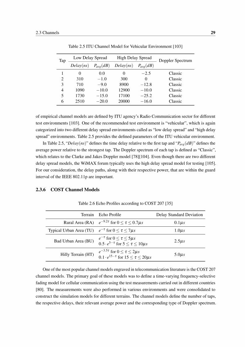
2.3 Channels 29
Table 2.5 ITU Channel Model for Vehicular Environment [103]
TapLow Delay Spread High Delay Spread
Doppler SpectrumDelay(ns) Pavg(dB) Delay(ns) Pavg(dB)
1 0 0.0 0 −2.5 Classic2 310 −1.0 300 0 Classic3 710 −9.0 8900 −12.8 Classic4 1090 −10.0 12900 −10.0 Classic5 1730 −15.0 17100 −25.2 Classic6 2510 −20.0 20000 −16.0 Classic
of empirical channel models are defined by ITU agency’s Radio Communication sector for differenttest environments [103]. One of the recommended test environment is “vehicular”, which is againcategorized into two different delay spread environments called as “low delay spread” and “high delayspread” environments. Table 2.5 provides the defined parameters of the ITU vehicular environment.
In Table 2.5, “Delay(ns)” defines the time delay relative to the first tap and “Pavg(dB)” defines theaverage power relative to the strongest tap. The Doppler spectrum of each tap is defined as “Classic”,which relates to the Clarke and Jakes Doppler model [78][104]. Even though there are two differentdelay spread models, the WiMAX forum typically uses the high delay spread model for testing [105].For our consideration, the delay paths, along with their respective power, that are within the guardinterval of the IEEE 802.11p are important.
2.3.6 COST Channel Models
Table 2.6 Echo Profiles according to COST 207 [35]
Terrain Echo Profile Delay Standard Deviation
Rural Area (RA) e−9.2τ for 0 ≤ τ ≤ 0.7µs 0.1µs
Typical Urban Area (TU) e−τ for 0 ≤ τ ≤ 7µs 1.0µs
Bad Urban Area (BU)e−τ for 0 ≤ τ ≤ 5µs
2.5µs0.5 · e5−τ for 5 ≤ τ ≤ 10µs
Hilly Terrain (HT)e−3.5τ for 0 ≤ τ ≤ 2µs
5.0µs0.1 · e15−τ for 15 ≤ τ ≤ 20µs
One of the most popular channel models engraved in telecommunication literature is the COST 207channel models. The primary goal of these models was to define a time-varying frequency-selectivefading model for cellular communication using the test measurements carried out in different countries[80]. The measurements were also performed in various environments and were consolidated toconstruct the simulation models for different terrains. The channel models define the number of taps,the respective delays, their relevant average power and the corresponding type of Doppler spectrum.

30 Foundations
An example of the channel models, also called as the Echo profiles, for different terrains is given inTable 2.6. Even though the profiles define delays up to 20µs, the IEEE 802.11p restricts the maximumdelay that can be compensated to just 1.6µs. COST 207 [80] went a step further and also definedthe tap settings that can be used by fading simulators. Example of a 6-Tap Typical Urban fadingsimulator is given in Table 2.7, which again defines certain taps beyond the guard interval of IEEE802.11p. It also defines the different categories of Doppler spectrum, ‘CLASS’ refers to the defaultDoppler spectrum which is nothing but the Jake’s Doppler model [78]. ‘GAUS1’ and ‘GAUS2’ arebi-Gaussian Doppler spectrum defined by the report [80]. The various models are already configuredin MATLAB under the ‘stdchan’ which is a part of the Communications System Toolbox, and can bedirectly invoked in the simulation platform for experimentation.
Table 2.7 COST 207 Fading Simulator Settings - Typical Urban [80]
Tap No. Delay (µs) Power (linear) Power (dB) Doppler Category SD(µs)
1 0 0.5 −3 CLASS
1.1
2 0.2 1 0 CLASS3 0.6 0.63 −2 GAUS14 1.6 0.25 −6 GAUS15 2.4 0.16 −8 GAUS26 5.0 0.1 −10 GAUS2
2.3.7 GSM/EDGE Channel Models
Table 2.8 GSM/EDGE Channel Model - Typical Urban 6 Taps [81]
Tap No. Delay (µs) Average relative power (dB) Doppler Category
1 0 −3 JAKES2 0.2 0 JAKES3 0.6 −2 JAKES4 1.6 −6 JAKES5 2.4 −8 JAKES6 5.0 −10 JAKES
Radio propagation in the mobile radio environment is described by highly dispersive multipathcaused by reflection and scattering [81]. The paths between base station and mobile station generallyconsist of large reflectors and/or scatterers which consequently generates a number of waves thatarrive in the vicinity of the mobile station with random amplitudes and delays. In order to simulatesuch effects, the 3rd Generation Partnership Project (3GPP) and ETSI organizations outlined channelmodels for GSM standard of digital cellular telecommunications system [81]. These models are basedon the COST 207 models, but the Doppler spectrum for all paths is restricted to the Jake’s Dopplermodel [78]. As an example, Table 2.8 demonstrates the similarity between these channel models and

2.4 MATLAB 31
the COST 207 channel models. However, the recommendation is to employ the 12 tap settings of eachterrain whenever possible, and utilize the 6 tap model exclusively under computational restrictions.The guard interval limitations of the IEEE 802.11p was highlighted for the COST 207 models insubsection 2.3.6, and is replicated here for the GSM/EDGE channel models too. Considering therecommended 12 tap channel models inflates the errors due to the irreparable ISI. Therefore, in thisthesis the channels are restricted and configured to generate delays that are within the prescribedguard interval.
2.4 MATLAB
MATLAB is a multi-paradigm numerical computing environment and fourth-generation programminglanguage. A proprietary programming language developed by MathWorks, MATLAB allows matrixmanipulations, plotting of functions and data, implementation of algorithms, creation of user interfaces,and interfacing with programs written in other languages, including C, C++, C#, Java, Fortran andPython [106]. Although the popularity of MATLAB has been consistent over many years [107], itis increasingly being overshadowed in favor of the Python programming language. However, theability of rapid prototyping and the large database of built-in algorithms which have been regularlyacknowledged by the research community, compliments its use for this thesis.
As mentioned in subsection 1.2.4, abundant research has been performed by implementingIEEE 802.11p standard on the MATLAB platform, but a flexible simulation platform that is readilydownloadable is nonexistent. This thesis reconstructs the simulation platform for IEEE 802.11p basedon the structural guidelines of DVB-T2 CSP. The DVB-T2 CSP has been developed collaborativelyby a number of organizations within the DVB consortium [73]. The structure is flexible enough toallow development and integration of custom channel estimation and equalization functions. Thishas been replicated in the simulation platform developed for this thesis and is also downloadable forfurther research [74]. Additionally, the documentation of MATLAB is extensive enough to assistany beginner to swiftly get accustomed to the environment. Therefore, the discussion on MATLABand its built-in functions is restricted in this thesis under the assumption that either the vast trove ofdocuments is readily available or that the reader is already comfortable with it.
2.5 GNU Radio
GNU Radio is a free and open-source software development tool-kit that provides signal processingblocks to implement software radios. It can be used with readily-available low-cost external RFhardware to create software-defined radios, or without hardware in a simulation-like environment.It is widely used in hobbyist, academic and commercial environments to support both wirelesscommunications research and real-world radio systems [108].
It has a graphical user interface called as the “GNU Radio Companion”, that has drag-and-dropsignal processing blocks that can be connected together to simulate basic signal processing operations.

32 Foundations
Custom-made blocks can be created and used in a similar way to build more complex and user-definedsignal processing schemes. To create custom blocks, one has to know C++ programming, as most ofthe performance critical blocks are written in C++. It is also important to mention that knowledgeof Python programming language, use of ‘CMakeLists’, and the working of Extensible MarkupLanguage (XML) files are essential to build a complete framework on the GNU Radio platform. Manyprotocols have been simulated on the GNU Radio, like Bluetooth, IEEE 802.15.4 or WPAN, andGSM. The use of GNU Radio with the USRP can help researchers in avoiding the closed sourcefirmware/drivers of commercial chip-sets by providing an ability for full customization at physicaland data-link layers [109].
2.5.1 IEEE 802.11p Model
One of the first implementations of IEEE 802.11 on GNU Radio, was developed by the AdaptiveDynamic Radio Open-Source Intelligent Team (ADROIT) project funded by the Defense AdvancedResearch Projects Agency (DARPA), Adaptive Cognition-Enhanced Radio Teams (ACERT) program.However, the implementation limited the bandwidth and has now become obsolete [110]. Recently,the entire transceiver for IEEE 802.11p has been developed [86], without any bandwidth restrictions,other than the restrictions defined by the standard itself. The software defined model of IEEE 802.11ptransceiver that has a software loop-back, named as “WiFi Loopback”, is shown in Figure 2.9.
Fig. 2.9 IEEE 802.11p Software Loopback [86]
The “Message Strobe” block creates the input message that is to be transmitted in a container calledas Polymorphic Types (PMT). PMT are opaque data types that are designed as generic containers ofdata that can be safely passed around between blocks and threads in GNU Radio. They are heavilyused in the stream tags and message passing interfaces [111]. The size of the message and therepetition rate can also be varied to test the system at different packet rates. The “WiFi MAC” blockputs the data message into the MAC frame according to the frame structure defined in the standard.

2.5 GNU Radio 33
These MAC frames are then passed onto a hierarchical block called as the “WiFi PHY Hier” whichcontains the PHY layer blocks of the standard. The flow-graph of this hierarchical block is shown inFigure 2.10.
Fig. 2.10 PHY Hierarchical Flowgraph [86]
The PMT messages, inside the defined MAC frames, are received by the “Pad Source” block,labeled as mac_in, as shown at the top of Figure 2.10. These frames containing the data is passedto the “WiFi Mapper”, where the data is passed through the scrambler and convolutional encoder.After convolutional encoding, the defined code puncturing method is applied, which is then fed to aninterleaver to finally output the stream of data in bytes. The output bytes are then fed to a “PacketHeader Generator” block and “Chunks to Symbols” block. The Packet Header Generator blockis used to generate a header for each packet including the addition of SIGNAL field described insubsection 2.2.6. The chunks to symbols block converts the incoming byte stream to the desired

34 Foundations
complex symbols based on the type of modulation that has been selected. The available choices formodulation is defined by standard and they are BPSK, Quadrature Phase Shift Keying (QPSK), 16Quadrature Amplitude Modulation (QAM), and 64 QAM. The complex symbols, along with thepacket headers, are the inputs to the “Tagged Stream Mux” block. This block collects the inputs,orders them sequentially with their respective stream tags and outputs them with a new length tagthat is the sum of all input length tags. It is important to note that this operation, like many other,might not be defined in the IEEE 802.11p standard, but is necessary in the GNU Radio environmentto produce precise synchronization.
The complex symbols, with their respective stream tags, are then fed to the “OFDM CarrierAllocator” block that takes the stream of complex, scalar modulation symbols and converts them intovectors which are the input for an IFFT in an OFDM transmitter. The defined values and positions ofthe Short Preamble, Long Preamble, and the pilots are used as ‘user settings’ in this block to generatea parallel stream for the IFFT. The “FFT” block is configured to perform IFFT while keeping the DCsub-carrier centered in the spectrum. These IFFT symbols are then collected by the “OFDM CyclicPrefixer”. This block adds a defined length of cyclic prefix and performs pulse shaping on OFDMsymbols. The stream of complex symbols, with the cyclic prefix, are now ready to be transmitted intothe channel. The “Pad Sink” block, labeled as samp_out connects back to the main flowgraph (“WiFiLoopback”).
Referring back to Figure 2.9, and tracing out the port labeled samp_out in “WiFi PHY Hier”,shows the port being connected to “Packet Pad2” block. This block adds a configurable numberof zeros before and after a burst. The burst has to be started and ended with a tag. It is handy forloop-back testing when there is no continuous sample stream. Furthermore, this block can add a tag toevery burst that lies a configurable number of seconds in the future. This is handy to buffer the samplestream for a short time to avoid under-runs during the transmission, which lead to corrupted signals[112]. This block is followed by the “Multiply Const” block, that just multiplies every complexsymbol with a set value defined by the desired SNR. The multiplication value from SNR is calculatedusing Equation 2.16.
Multiply Const =√
10SNR10 (2.16)
The complex symbol stream is then fed as input to the “Channel Model” which allows the user toset the voltage of an AWGN noise source, a normalized frequency offset, and a sample timing offset.The default settings only simulate a pure AWGN noise channel without any multi-path or Dopplereffects. The block can be replaced with other channel models to simulate the complex channelsexperienced in the vehicular environment. Once the complex stream has passed through the channel,the receiver receives these signals in the PHY layer, therefore we go back to the “WiFi PHY Hier”hierarchical block through the port samp_in. Inside the hierarchical block, Figure 2.10, after thesamp_in port, synchronization using the Short Preamble is performed. The structure of the ShortPreamble in IEEE 802.11p is explained in subsection 2.2.1. Auto-correlation of the Short Preamble is
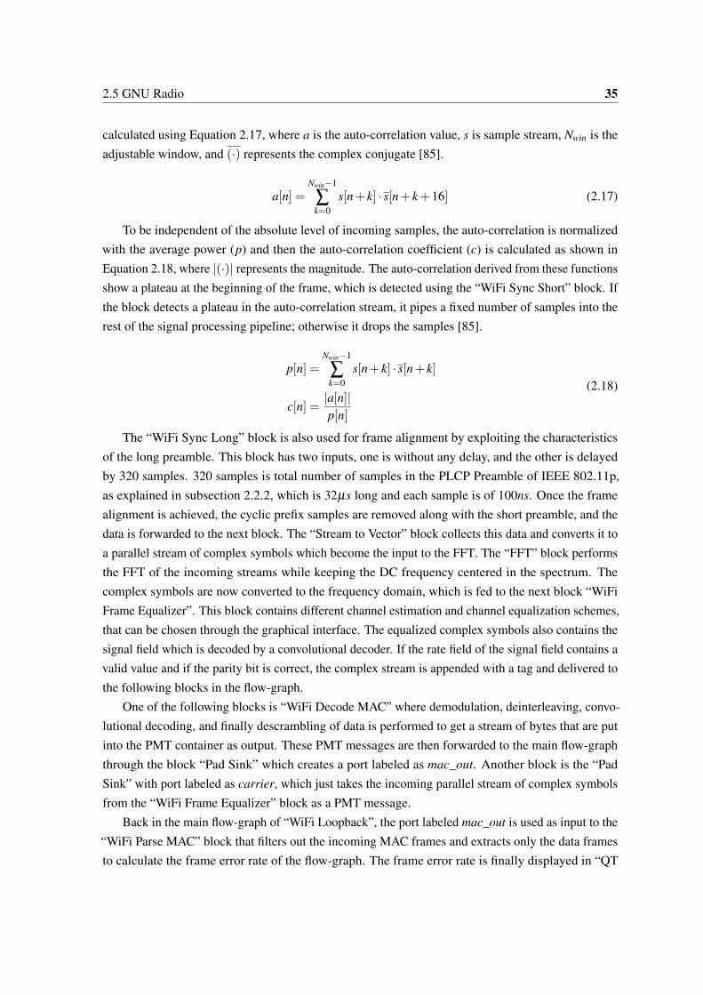
2.5 GNU Radio 35
calculated using Equation 2.17, where a is the auto-correlation value, s is sample stream, Nwin is theadjustable window, and (·) represents the complex conjugate [85].
a[n] =Nwin−1
∑k=0
s[n+ k] · s[n+ k+16] (2.17)
To be independent of the absolute level of incoming samples, the auto-correlation is normalizedwith the average power (p) and then the auto-correlation coefficient (c) is calculated as shown inEquation 2.18, where |(·)| represents the magnitude. The auto-correlation derived from these functionsshow a plateau at the beginning of the frame, which is detected using the “WiFi Sync Short” block. Ifthe block detects a plateau in the auto-correlation stream, it pipes a fixed number of samples into therest of the signal processing pipeline; otherwise it drops the samples [85].
p[n] =Nwin−1
∑k=0
s[n+ k] · s[n+ k]
c[n] =|a[n]|p[n]
(2.18)
The “WiFi Sync Long” block is also used for frame alignment by exploiting the characteristicsof the long preamble. This block has two inputs, one is without any delay, and the other is delayedby 320 samples. 320 samples is total number of samples in the PLCP Preamble of IEEE 802.11p,as explained in subsection 2.2.2, which is 32µs long and each sample is of 100ns. Once the framealignment is achieved, the cyclic prefix samples are removed along with the short preamble, and thedata is forwarded to the next block. The “Stream to Vector” block collects this data and converts it toa parallel stream of complex symbols which become the input to the FFT. The “FFT” block performsthe FFT of the incoming streams while keeping the DC frequency centered in the spectrum. Thecomplex symbols are now converted to the frequency domain, which is fed to the next block “WiFiFrame Equalizer”. This block contains different channel estimation and channel equalization schemes,that can be chosen through the graphical interface. The equalized complex symbols also contains thesignal field which is decoded by a convolutional decoder. If the rate field of the signal field contains avalid value and if the parity bit is correct, the complex stream is appended with a tag and delivered tothe following blocks in the flow-graph.
One of the following blocks is “WiFi Decode MAC” where demodulation, deinterleaving, convo-lutional decoding, and finally descrambling of data is performed to get a stream of bytes that are putinto the PMT container as output. These PMT messages are then forwarded to the main flow-graphthrough the block “Pad Sink” which creates a port labeled as mac_out. Another block is the “PadSink” with port labeled as carrier, which just takes the incoming parallel stream of complex symbolsfrom the “WiFi Frame Equalizer” block as a PMT message.
Back in the main flow-graph of “WiFi Loopback”, the port labeled mac_out is used as input to the“WiFi Parse MAC” block that filters out the incoming MAC frames and extracts only the data framesto calculate the frame error rate of the flow-graph. The frame error rate is finally displayed in “QT
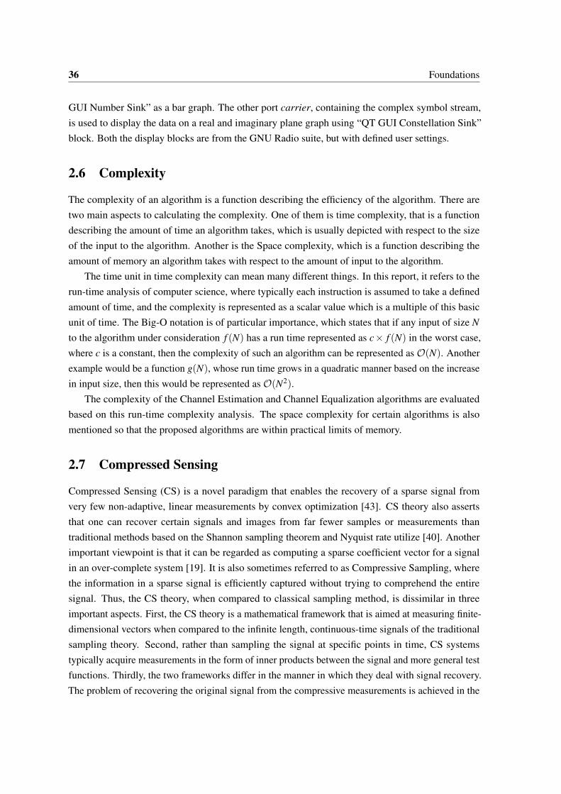
36 Foundations
GUI Number Sink” as a bar graph. The other port carrier, containing the complex symbol stream,is used to display the data on a real and imaginary plane graph using “QT GUI Constellation Sink”block. Both the display blocks are from the GNU Radio suite, but with defined user settings.
2.6 Complexity
The complexity of an algorithm is a function describing the efficiency of the algorithm. There aretwo main aspects to calculating the complexity. One of them is time complexity, that is a functiondescribing the amount of time an algorithm takes, which is usually depicted with respect to the sizeof the input to the algorithm. Another is the Space complexity, which is a function describing theamount of memory an algorithm takes with respect to the amount of input to the algorithm.
The time unit in time complexity can mean many different things. In this report, it refers to therun-time analysis of computer science, where typically each instruction is assumed to take a definedamount of time, and the complexity is represented as a scalar value which is a multiple of this basicunit of time. The Big-O notation is of particular importance, which states that if any input of size Nto the algorithm under consideration f (N) has a run time represented as c× f (N) in the worst case,where c is a constant, then the complexity of such an algorithm can be represented as O(N). Anotherexample would be a function g(N), whose run time grows in a quadratic manner based on the increasein input size, then this would be represented as O(N2).
The complexity of the Channel Estimation and Channel Equalization algorithms are evaluatedbased on this run-time complexity analysis. The space complexity for certain algorithms is alsomentioned so that the proposed algorithms are within practical limits of memory.
2.7 Compressed Sensing
Compressed Sensing (CS) is a novel paradigm that enables the recovery of a sparse signal fromvery few non-adaptive, linear measurements by convex optimization [43]. CS theory also assertsthat one can recover certain signals and images from far fewer samples or measurements thantraditional methods based on the Shannon sampling theorem and Nyquist rate utilize [40]. Anotherimportant viewpoint is that it can be regarded as computing a sparse coefficient vector for a signalin an over-complete system [19]. It is also sometimes referred to as Compressive Sampling, wherethe information in a sparse signal is efficiently captured without trying to comprehend the entiresignal. Thus, the CS theory, when compared to classical sampling method, is dissimilar in threeimportant aspects. First, the CS theory is a mathematical framework that is aimed at measuring finite-dimensional vectors when compared to the infinite length, continuous-time signals of the traditionalsampling theory. Second, rather than sampling the signal at specific points in time, CS systemstypically acquire measurements in the form of inner products between the signal and more general testfunctions. Thirdly, the two frameworks differ in the manner in which they deal with signal recovery.The problem of recovering the original signal from the compressive measurements is achieved in the

2.7 Compressed Sensing 37
Nyquist-Shannon framework through ‘sinc’ interpolation which is a linear process. In CS, however,signal recovery is typically achieved using highly nonlinear methods [43].
The fundamental papers that introduced compressed sensing [49][113] were utilized for randomsensing matrices, since they allowed for a minimal number of non-adaptive and linear measurements.However, as mentioned above, the term CS also encompasses ‘Sparse Recovery’ [19]. The sparsityconsideration, that is the central notion to CS theory, is applicable to the wireless channels whereonly few dominant echoes are anticipated. In wireless communication, most channel models definelarge delay spreads with only a few dominant echoes as shown in subsection 2.3.5, subsection 2.3.6and subsection 2.3.7. Therefore, the sparsity assumption is indeed reasonable for wireless channels,as is the case for most natural phenomenon. Exploiting this sparsity and adopting the CS methodsfor the ’Hilly Terrain’ has already generated more than 10dB improvement in SNR [114]. Even formore adverse underwater acoustic channels, the CS methods offer an uniform gain over other methods[20]. As an example, let a matrix ΦΦΦ contain the signals corresponding to all the different delay pathsthat could occur in a channel. At the receiver, only a small set of these delay paths will superimpose,which can be represented as Equation 2.19 [52].
yyy = ΦΦΦxxx (2.19)
Here yyy is the received signal, xxx represents the index/coefficient of dominant delay paths thatsuperimpose at the receiver which inherently contains only few non-zero values. If S represents thetotal number of indices in ΦΦΦ, then card(supp(xxx)) ≪ S, where supp represents the support of thevector, and card represents the cardinality of the set of non-zero values. As a result, xxx is innatelysparse which the CS methods attempt to recover. One of the categories of CS that deal with recoveryof this sparse representation is called as ‘Greedy Algorithms’. While convex optimization techniquesare powerful methods for computing sparse representations, there are also a variety of greedy/iterativemethods for solving such problems. Greedy algorithms rely on iterative approximation of the signalcoefficients and support, either by iteratively identifying the support of the signal until a convergencecriterion is met, or alternatively by obtaining an improved estimate of the sparse signal at each iterationthat attempts to account for the mismatch to the measured data. Some greedy methods can actually beshown to have performance guarantees that match those obtained for convex optimization approaches.In fact, some of the more sophisticated greedy algorithms are remarkably similar to those used for ℓ1
minimization. However, the techniques required to prove performance guarantees are substantiallydifferent [43].
Additionally, these methods precedes CS, and were utilized in many fields including geophysics,communication, statistics and theoretical computer science before the term compressed sensing wasever coined. It is important to note that these algorithms have been popular because of its ease ofimplementation and low computational complexity. Consequently, it could also fail to find the sparsestsolution in certain scenarios [115]. In various methods and scenarios, the ℓ1-norm relaxation leads toa solution that is not exactly sparse and results in numerous negligible values that don’t contribute

38 Foundations
significantly to the estimation error [115]. This is generally solved by a stopping criterion that isdesigned to halt the iterative process of these greedy algorithms to achieve the exact sparse solution.But, such ambitious goal of achieving the exact sparsity is often impractical. Instead, the sparsestsolution containing the most dominant components can be guaranteed [116].
In conclusion, the CS schemes are increasingly being used to estimate a doubly selective channel[16][18][22]. The wireless communication channel is inherently sparse and CS based channelestimation schemes exploit this sparsity to make significant gains in complexity. This thesis restrictsitself to the investigation and evaluation of a subset of greedy CS algorithms called as matchingpursuit. Building on these foundations, improvements to the algorithm are proposed and evaluated inthe context of channel estimation for the IEEE 802.11p standard.
2.8 Channel Estimation
OFDM systems, with higher data rates, require the channel information for coherent demodulation.The channel estimation schemes can be broadly divided into three categories [98]. One of thecategory is the blind or semi-blind estimation methods which are used sparingly due to their highcomputational demand. Another category is the use of decision-directed procedure in which virtualpilots are obtained from the demodulated/decoded information. The third category makes use ofthe pilot sub-carriers within the OFDM symbol, where the transmitter and the receiver know theinformation on the pilots. Using this information, the multiplicative complex factors can be extractedfrom the received symbols at the pilot sub-carriers, and then interpolated to other sub-carriers toyield a complete channel estimate at each sub-carrier. This category of channel estimation is whatis considered in this report, where we have a defined set of pilots. In the case of IEEE 802.11p, thepreamble is typically utilized to estimate the channel both in the frequency and the time domain.
2.8.1 Least Squares
The LS channel estimation scheme is computationally simple, that provides adequate channel esti-mation information for indoor environments. Consequently, they are one of the most widely usedestimation schemes implemented on hardware. In IEEE 802.11, the two long preambles in the PLCPPreamble are used to estimate the channel. The two received long preambles in frequency domain,denoted by yyyL1 ∈CN and yyyL2 ∈CN , are divided by the known transmitted preamble xxxL ∈CN and thenaveraged to obtain the LS estimate of the channel, as shown in Equation 2.20. Here N denotes theFFT length, and C denotes the complex space.
h f [n] =yL1[n]+ yL2[n]
2 · xL[n], hhh f ∈ CN (2.20)
Here hhh f is a vector that is the LS estimate of the channel in frequency domain, which are justcomplex coefficients for each sub-carrier. The averaging of the two preambles, instead of consideringjust a single long preamble, to estimate the channel improves the performance of the LS estimator

2.8 Channel Estimation 39
under low SNR conditions. The advantage of the LS estimator is its exceptionally low complexity andit performs exceedingly well under purely AWGN channel conditions [37]. However, under highlymobile environments the performance of LS estimator is inadequate.
2.8.2 Basic Matching Pursuit
Matching pursuit refers to a family of algorithms that generate a set of bases for representing the signalin a greedy fashion [117]. Representing the signal in unique set of basis functions also involves findingthe coefficients for those basis functions. The ability of a basis to provide a sparse representationdepends on how well the signal characteristics match the characteristics of the basis vectors. Forexample, smooth continuous signals are sparsely represented in a Fourier basis, while impulses arenot. A smooth signal with isolated discontinuities is sparsely represented in a wavelet basis. However,a wavelet basis is not efficient at representing a signal whose Fourier transform has narrow highfrequency support [118]. The effects of the channel on the signal does not permit sparse representationin any single basis. The Matching Pursuit algorithms allows you to build a set of basis that can bea combination of different bases, which is called as the dictionary. The dictionary contains vectorsthat are basis functions in the signal space, that represent the different time-frequency effects ofthe channel. The signal is then represented only by a subset of these customized basis functionsafter adopting the MP algorithm, which implies that a sparse representation of the signal using thedictionary elements has been achieved.
CS builds upon the fundamental fact that many signals can be represented using only a fewnon-zero coefficients in a suitable basis or dictionary [43]. Linear combination of these suitable basesand their corresponding non-zero coefficients can then enable recovery of such signals from veryfew measurements. CS theory asserts that one can recover certain signals and images from far fewersamples or measurements than traditional methods like Nyquist sampling [40]. CS sounds a lot likeMP, in fact, CS is a more recent theoretical framework that deals with sparse recovery of signalswhich also encompasses the pre-dated MP algorithms.
Matching pursuit is a greedy algorithm that computes the best linear approximation to a signalin a complete, redundant dictionary. However, in comparison to other sparse recovery methods,like ℓp-norm regularized method, the MP algorithms are computationally more efficient but remainanalytically less tractable [20]. The prerequisite step in a MP algorithm is building the set of basisvectors called as the dictionary. In this thesis, the dictionary must represent how the long preambleis affected by the channel perturbations. Hence, the known vector of long preamble is corrupted bythe different values of delay and Doppler to form different atoms of the dictionary. Once we havethe complete dictionary, the received long preamble is compared with the atoms in the dictionaryto find the best correlating atom in each iteration. The delay and Doppler values that were used tocorrupt this chosen atom of the dictionary is considered as the delay and Doppler that the signal hasexperienced when passing through the channel. The atoms can be considered to be different columns

40 Foundations
of the dictionary, where each column then becomes the long preamble corrupted by the respectivedelay and Doppler values.
To illustrate the methodology of building the dictionary, consider a channel that has a definedmaximum delay and a constrained maximum Doppler shift. Consider that the channel can have amaximum of τ delay, and a maximum Doppler shift of fd . An integer value representing the maximumdelay τ can be defined as K = τ/∆τ , where ∆τ is the minimum delay resolution and can be as smallas 1ns. Similarly, an integer value representing the maximum Doppler shift fd can be defined asL = fd/(∆ f ), where ∆ f is the minimum delay resolution and is usually considered to be 1Hz. Thenthe dictionary DDD, in the simplest form, must contain K ×L vectors. Each vector must be equal to thelength of the long preamble, which is equal to the length of FFT: N. The long preamble is in thecomplex space, hence each element of the dictionary dddk,l ∈ CN , where k ∈ 0 · · ·K and l ∈ 0 · · ·L.ddd is a vector, and dddk,l represents the dictionary atom corresponding to kth delay and lth Doppler shift.The dictionary atoms can also be written in the form of Equation 2.21, where lllp is the transmittedpreamble in the frequency domain [55].
dddk,l = HHH f lllp
dddk,l =
(K−1
∑k=0
L−1
∑l=0
UUUk,lCCClΛΛΛk
)lllp
(2.21)
The channel matrix HHH f , as shown in Equation 2.21, can be split into its respective components.UUUk,l are complex coefficients representing the different attenuation experienced by the signal alongthe different paths. CCCl is the circular Doppler shift matrix in the frequency domain. ΛΛΛk is the diagonaldelay matrix also in the frequency domain. When the size of the delay search and Doppler search islarge, then the size of the dictionary is huge. It would be impractical to search through all the elementsof such a large dictionary to find the best correlating atom in each iteration of the MP algorithm.Exploiting the knowledge of the structure and position of the long preamble, along with adaptivesearch techniques can reduce the complexity to a great extent [51].
Once the dictionary has been created, it is taken as one of the inputs in the BMP algorithm. TheBMP algorithm is an iterative procedure which can sequentially identify the dominant channel tapsand estimate the associated tap coefficients. At each iteration, it selects one column of the dictionarythat correlates best with the approximation residual from the previous iteration [20]. The differentsteps of the BMP algorithm is shown in Table 2.9.
The initialization step is building the dictionary, where the different atoms of the dictionaryrepresent different values of delay and Doppler. Equation 2.22 is to store the received long preambleyyy as the residual vector rrr0. Equation 2.23 is to compute the rank-one projections of the residualvector rrr0 on all the atoms of the dictionary DDD. Here, each atom is a vector which is represented asddd j, where j is an index denoting the respective column. The atom corresponding to the maximalrank-one projection is calculated using Equation 2.24. Here, ∥(·)∥2 represents the ℓ2-Norm. Theindex relating to this maximum rank-one projection s1 is stored into a set iii1 in Equation 2.25. The

2.8 Channel Estimation 41
Table 2.9 BMP Algorithm
Initialization
rrr0 = yyy (2.22)
b0, j = dddHj rrr0, for j = 1 · · ·KL (2.23)
s1 = arg maxj=1···KL
|b0, j|2∥ddd j∥2
2
(2.24)
iii1 = s1 (2.25)
x1 =b0,s1
∥ddds1∥22
(2.26)
b1, j = b0, j − x1dddHj ddds1 , for j = 1 · · ·KL, j /∈ iii1 (2.27)
the pth iteration, p > 1
sp = arg maxj=1···KL, j/∈iiip−1
|bp−1, j|2∥ddd j∥2
2
(2.28)
iiip = iiip−1,sp (2.29)
xp =bp−1,sp
∥dddsp∥22
(2.30)
bp, j = bp−1, j − xpdddHj dddsp , for j = 1 · · ·KL, j /∈ iiip (2.31)
indexes of atoms for further iterations are also updated in this set. In Equation 2.26, x1 representsthe coefficient related to the dictionary atom that was selected in Equation 2.24. It gives a measureof the correlation between the residual vector rrr0 and the chosen atom of the dictionary. Once the x1
value is calculated, the rank-one projections calculated in Equation 2.23 are updated to remove thecontribution of the found dictionary atom on the projections in Equation 2.27. The x1 value can also beused to update the residual vector, if needed. For the following iterations of the algorithm, the updatedrank one projection values bp−1, j is used to calculate the next maximal rank-one projection atom inEquation 2.28 while ignoring the atoms found in previous iterations. Equation 2.29, Equation 2.30and Equation 2.31 update the set of found atoms, calculate the coefficient of the dictionary atom andfinally update the rank-one projection values, respectively.
The algorithm is stopped based on a stopping criterion, which can be just number of iterations ora more complicated method of calculating the residual error [119]. The residual vector, which is the

42 Foundations
vector remaining after removing the contribution of the found atom from the received vector, can becomputed using Equation 2.32. The initialization of the residual vector is the same as in Equation 2.22in the algorithm, which is rrr0 = yyy.
rrrp = rrrp−1 − xpdddsp (2.32)
The BMP, once completed, gives a sparse representation of the received long preamble in theterms of the dictionary atoms and their respective coefficients. Using these atoms and coefficients, thechannel matrix can be constructed, that can be used by the following channel equalization scheme tocorrect the received symbols. The BMP performs a search through all the atoms of the dictionary ateach iteration and within each iteration the computational complexity is proportional to the size ofthe vector, which in this thesis is equal to the FFT size. Therefore, the complexity of the entire BMPalgorithm is O(KLqN) [20], where K, as mentioned before, is the number of delays to be consideredfor the delay search, L is the number of Doppler frequencies to be considered for the Doppler search,N is the FFT size and q is the total number of dominant paths that are found which is analogous to thenumber of iterations of the BMP algorithm.
2.8.3 Orthogonal Matching Pursuit
The dictionary, in the initialization step of the BMP algorithm (Table 2.9), is assumed to have differentatoms that are orthogonal to each other. This orthogonality, if maintained between the atoms, results inproducing accurate xp values in Equation 2.30 of the algorithm. Once we have accurate xp, updatingthe rank-one projections bp, j in Equation 2.31 of the algorithm is also systematically correct. However,orthogonality between atoms cannot be always guaranteed, and in such cases the xp values and thecorresponding revision of the bp, j values are incorrect, resulting in inaccurate minimum residual error.Hence, to overcome this drawback of BMP, the OMP algorithm was proposed.
The OMP algorithm just changes the calculation of xp values in Equation 2.26 and Equation 2.30of the BMP algorithm. The equation to calculate the values of xp in OMP is given in Equation 2.33[20]. It is important to note that DDDs,p ≜
[ddds1 · · ·dddsp
], which is a matrix of all the dictionary atoms
selected by the algorithm till and including the pth iteration.
xxxp,omp = arg minxxx,yyy∈CN
∥yyy−DDDs,pxxx∥22
=[DDDH
s,pDDDs,p]−1
DDDHs,pyyy
(2.33)
Equation 2.33 is the LS minimization based on the atoms selected at each iteration. Here, (·)−1
represents the inverse of a matrix. In comparison to the BMP algorithm, the xp values calculated inOMP give a better estimate of the coefficient with respect to the dictionary atoms when the atoms arenot orthogonal to each other.

2.8 Channel Estimation 43
The working of the OMP might become a little bit more clear by considering a simple example.Consider a received vector defined as
yyy =[0 0 0 1 1 −2
]T
where (·)T means the transpose of the vector, which implies that yyy is a column vector. To build adictionary one must consider all possible combinations, but for the sake of simplicity, let’s consideronly a subset. The dictionary is given by
DDD =
0 1 1 −1 −1 0 −1 0 −1 0−1 −1 0 1 −1 0 0 −1 0 11 −1 1 −1 0 −1 1 1 0 01 0 −1 0 0 1 −1 −1 1 1−1 0 0 0 1 0 1 0 1 −10 0 −1 −1 −1 0 −1 1 −1 0
The conjugate transpose is represented as (·)H . DDDH is nothing but the transpose of the matrix as all ofthem are real values. Multiplying DDDH and yyy gives
bbb0 = dddHj rrr0, for j = 1 · · ·KL
bbb0 = DDDHyyy
bbb0 =[0 0 1 2 3 1 2 −3 4 0
]T
The maximum value in the vector bbb0 is 4, which means that the maximization step is given as
s1 = arg maxj=1···KL
∣∣b0, j∣∣2∥∥ddd j∥∥2
2
≈ 4
Thus, the column 9 of the dictionary DDD has best rank-one projection of the received vector yyy. Thereforethe set of indices is given as
iii1 = s1= 9
This means that for further calculations in the first iteration, the 9th column of the dictionary isconsidered.
ddd9 =[−1 0 0 1 1 −1
]T
For updating the residual vector, x value is needed. To simplify the calculations, let’s consider
x1 = 1
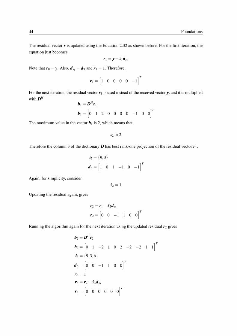
44 Foundations
The residual vector rrr is updated using the Equation 2.32 as shown before. For the first iteration, theequation just becomes
rrr1 = yyy− x1ddds1
Note that rrr0 = yyy. Also, ddds1 = ddd9 and x1 = 1. Therefore,
rrr1 =[1 0 0 0 0 −1
]T
For the next iteration, the residual vector rrr1 is used instead of the received vector yyy, and it is multipliedwith DDDH
bbb1 = DDDHrrr1
bbb1 =[0 1 2 0 0 0 0 −1 0 0
]T
The maximum value in the vector bbb1 is 2, which means that
s2 ≈ 2
Therefore the column 3 of the dictionary DDD has best rank-one projection of the residual vector rrr1.
iii2 = 9,3
ddd3 =[1 0 1 −1 0 −1
]T
Again, for simplicity, considerx2 = 1
Updating the residual again, gives
rrr2 = rrr1 − x2ddds2
rrr2 =[0 0 −1 1 0 0
]T
Running the algorithm again for the next iteration using the updated residual rrr2 gives
bbb2 = DDDHrrr2
bbb2 =[0 1 −2 1 0 2 −2 −2 1 1
]T
iii3 = 9,3,6
ddd6 =[0 0 −1 1 0 0
]T
x3 = 1
rrr3 = rrr2 − x3ddds3
rrr3 =[0 0 0 0 0 0
]T

2.8 Channel Estimation 45
Notice that the final residual vector rrr3 contains all zeros, which means that the received vector yyy cannow be represented completely by the 3 chosen columns of the dictionary given in iii3. However, itis also important to note that this wouldn’t have worked so neatly if other columns were chosen atany iteration, and this might be the case when two columns can give similar maximum values upto acertain limit of resolution. Periodically, the residual vector might not result in all zeros, which mightalso be the case when incomplete dictionaries are considered. In such cases, the stopping criterionevaluates the residual vector and stops the algorithm based on a predefined condition. Nevertheless,the computational complexity for the OMP algorithm remains the same as that of the BMP algorithm,which is O(KLqN) [20]. The additional complexity of calculating the inverse of a matrix, shown inEquation 2.33, is insignificant under the assumption that q ≪ K, which is nothing but the underlyingconcept of CS based schemes.
2.8.4 Alternate Matching Pursuit Algorithms
In this section, the alternative methods of MP like Subspace Pursuit (SP), Compressive SamplingMatched Pursuit (CoSaMP), Stagewise Orthogonal Matching Pursuit (StOMP), Regularized Orthogo-nal Matching Pursuit (ROMP) and Sparsity Adaptive Matching Pursuit (SAMP) are explored and theirrelevance to the channel estimation of doubly selective channel is investigated. The advantages anddisadvantages of these methods over the BMP and OMP are also highlighted. The matching pursuitalgorithms, BMP and OMP, introduced above are configured to find the support of the unknownsignal sequentially. At each iteration of the algorithms, one of the vector from the dictionary isselected for testing based on the correlation values between the columns of the dictionary and thereceived vector. If deemed sufficiently reliable, the candidates are subsequently added to the currentestimate of the support set. The pursuit algorithms iterate this procedure until all the coordinates inthe correct support are in the estimated support. The computational complexity of the MP strategiesdepends on the number of iterations needed for exact reconstruction. If the channel is characterizedby a sparsity of q, meaning that it has q delay paths then the MP algorithms always run through qiterations, and therefore its complexity is O(KLqN). This complexity is significantly smaller thanthat of certain Linear Programming (LP) methods of CS [52], especially when the signal sparsity levelq is small. However, the pursuit algorithms do not have provable reconstruction quality of the levelof LP methods. For OMP to operate successfully, one requires that the correlation or inner productsbetween a set of q different atoms of the dictionary is less than 1/2 [50].
However, the SP is based on a more relaxed constraint called as the Restricted Isometry Property(RIP) [52]. The RIP is dependent on the dictionary DDD ∈ CN×KL which contains the complete setof vectors. If DDDq ∈ CN×q represents all the combinations of q vectors within the dictionary, andxxxq ∈ Cq×1 represents all possible combination of the complex coefficients within these q vectors, thenthe RIP is given by Equation 2.34 [19], where δ ∈ (0,1).
(1−δ )∥∥xxxq∥∥2
2 ≤∥∥DDDqxxxq
∥∥22 ≤ (1+δ )
∥∥xxxq∥∥2
2 (2.34)
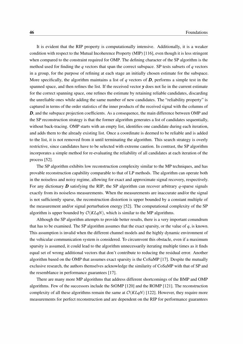
46 Foundations
It is evident that the RIP property is computationally intensive. Additionally, it is a weakercondition with respect to the Mutual Incoherence Property (MIP) [116], even though it is less stringentwhen compared to the constraint required for OMP. The defining character of the SP algorithm is themethod used for finding the q vectors that span the correct subspace. SP tests subsets of q vectorsin a group, for the purpose of refining at each stage an initially chosen estimate for the subspace.More specifically, the algorithm maintains a list of q vectors of DDD, performs a simple test in thespanned space, and then refines the list. If the received vector yyy does not lie in the current estimatefor the correct spanning space, one refines the estimate by retaining reliable candidates, discardingthe unreliable ones while adding the same number of new candidates. The “reliability property” iscaptured in terms of the order statistics of the inner products of the received signal with the columns ofDDD, and the subspace projection coefficients. As a consequence, the main difference between OMP andthe SP reconstruction strategy is that the former algorithm generates a list of candidates sequentially,without back-tracing. OMP starts with an empty list, identifies one candidate during each iteration,and adds them to the already existing list. Once a coordinate is deemed to be reliable and is addedto the list, it is not removed from it until terminating the algorithm. This search strategy is overlyrestrictive, since candidates have to be selected with extreme caution. In contrast, the SP algorithmincorporates a simple method for re-evaluating the reliability of all candidates at each iteration of theprocess [52].
The SP algorithm exhibits low reconstruction complexity similar to the MP techniques, and hasprovable reconstruction capability comparable to that of LP methods. The algorithm can operate bothin the noiseless and noisy regime, allowing for exact and approximate signal recovery, respectively.For any dictionary DDD satisfying the RIP, the SP algorithm can recover arbitrary q-sparse signalsexactly from its noiseless measurements. When the measurements are inaccurate and/or the signalis not sufficiently sparse, the reconstruction distortion is upper bounded by a constant multiple ofthe measurement and/or signal perturbation energy [52]. The computational complexity of the SPalgorithm is upper bounded by O(KLqN), which is similar to the MP algorithms.
Although the SP algorithm attempts to provide better results, there is a very important conundrumthat has to be examined. The SP algorithm assumes that the exact sparsity, or the value of q, is known.This assumption is invalid when the different channel models and the highly dynamic environment ofthe vehicular communication system is considered. To circumvent this obstacle, even if a maximumsparsity is assumed, it could lead to the algorithm unnecessarily iterating multiple times as it findsequal set of wrong additional vectors that don’t contribute to reducing the residual error. Anotheralgorithm based on the OMP that assumes exact sparsity is the CoSaMP [17]. Despite the mutuallyexclusive research, the authors themselves acknowledge the similarity of CoSaMP with that of SP andthe resemblance in performance guarantees [17].
There are many more MP algorithms that address different shortcomings of the BMP and OMPalgorithms. Few of the successors include the StOMP [120] and the ROMP [121]. The reconstructioncomplexity of all these algorithms remain the same at O(KLqN) [122]. However, they require moremeasurements for perfect reconstruction and are dependent on the RIP for performance guarantees

2.9 Channel Equalization 47
[122]. These algorithms don’t assume that the sparsity q is known, which is in contrast to the SP andCoSaMP. Another greedy algorithm called the SAMP is also designed for blind signal recovery whenthe exact sparsity q is unknown. It follows stage by stage estimation of the sparsity level to find thetrue support set of the target signals [122]. SAMP is a generalization of existing greedy algorithmsas both the OMP and the SP can be viewed as its special cases. As a result, the constraints on thedictionary is similar to OMP and offers performance that is comparable to SP. SAMP is mainly atrade-off between the algorithms based on the knowledge of known sparsity and the algorithms basedon unknown sparsity. In this thesis, although the applicability of few of the above algorithms are valid,they are not investigated further due to brevity and is appropriately highlighted as part of the futurework in section 5.2.
2.9 Channel Equalization
Channel Equalization can be broadly classified into two categories, coherent and non-coherentequalization. In non-coherent equalization, the receiver doesn’t use the channel information providedby the channel estimation techniques to equalize the symbols. In coherent equalization, informationof the channel characteristics provided by the channel estimation methods are used to equalize thesymbols. The accuracy of the channel estimation techniques contributes heavily to the accuracy of thechannel equalization techniques. The information, like phase and attenuation changes, of the channelis provided to the channel equalizer. The channel equalizer then uses this information to correct thesymbols, which have undergone perturbations like phase and attenuation changes.
2.9.1 One-Tap Equalizer
In most OFDM systems, the coherence bandwidth of the channel is assumed to be much larger thanthe bandwidth of the sub-carriers of an OFDM symbol. It also assumes that the coherence time of thechannel is much larger than the symbol period. This means that the channel is mainly stationary or flatfor the duration of the symbol period. Under such conditions, only a delay and change in amplitudeof the symbol can occur, which means that the perturbations of the channel can be represented bya single complex number. These variations can be equalized by a single delay and a gain for eachsub-carrier, and hence the name One-Tap Equalizer.
The One-Tap Equalization is done in the frequency domain. It requires the frequency domaininformation of delay and attenuation of the channel experienced by each sub-carrier. Generally, thesecomplex numbers are provided by the LS channel estimator shown in subsection 2.8.1. Let yyy ∈ CN
denote the received long preamble, where N = FFT Length. The channel response provided by theLS estimator is a also a vector, which is given as hhh f ∈ CN . Then, the One-Tap equalizer just divides

48 Foundations
the received vector by the channel response to equalize the symbols. This is shown in Equation 2.35,where yyy represents the equalized symbols.
yyy =yyy
hhh f(2.35)
The One-Tap equalizer along-with the LS estimator is sometimes referred to as LMS equalizer.The complexity of this equalizer is minimal as it is a single operation of division on each sub-carrier.But, with such low complexity, the performance of the equalizer is also limited. This equalizerassumes that the channel is mainly flat, which is not the case in vehicular networks. Under highlymobile environments, where multi-path and Doppler shifts are the norm, the performance of theOne-Tap equalizer is consistently inadequate when combined with a simple channel estimation schemelike LS.
2.9.2 Linear Minimum Mean Square Error Equalizer
The LMMSE equalizer attempts to equalize the symbols by minimizing the error between the receivedvector yyy and the known long preamble. The performance of the LMMSE equalizer is better thanthe One-Tap equalizer, but at the cost of higher complexity. Consider a complete channel matrixHHH ∈ CN×N , the received vector yyy ∈ CN , the transmitted preamble as xxx ∈ CN and the noise vector aszzz ∈ CN . Then the entire system can be represented by Equation 2.36.
yyy = HHHxxx+ zzz (2.36)
If the received vector and the transmitted preamble are the same, then there is no error that hasoccurred while passing through the channel. However, this is rarely the case, errors do occur frequentlyand our goal is to minimize these errors using the channel estimation and channel equalizationtechniques. The minimization of the mean square error between the received vector and the transmittedpreamble is then given by Equation 2.37, where GGG ∈ CN×N is an equalizer matrix.
MMSE = arg miny
∥xxx−GGGyyy∥22 (2.37)
In the above equation, it is assumed that the equalizer matrix is known. The linear solution for yyy,which is also called as linear least squares regression solution, is given by the Equation 2.38. Here,yyy denotes the LMMSE estimate of the received vector. The derivation of this equation is shown inAppendix section B.1.
yyy =(GGGHGGG
)−1GGGHxxx (2.38)
From Equation 2.38, it is evident that the knowledge of the channel matrix is omitted. Toincorporate the channel estimation scheme input into the LMMSE equalizer, assume that the channelmatrix provided by the channel estimation scheme is a N×N matrix, denoted by HHH, where N is the FFT
2.9 Channel Equalization 49
length. Then the above equation can be changed to Equation 2.39 [123], where σ2n denotes the noise
power, and IIIN denotes a N ×N identity matrix. The equation is similar to ridge regression solutionshown in Appendix section B.2, which tries to obtain a unique solution compared to Equation 2.38.
yyy = HHHH (HHHHHHH +σ2n IIIN)−1
xxx (2.39)
If SNR denotes the signal to noise ratio at the receiver, then the above equation can be rewrittenas Equation 2.40.
yyy = HHHH(
HHHHHHH +N
SNRIIIN
)−1
xxx (2.40)
In the above equation, the vector xxx can be replaced by the received vector yyy for OFDM symbolsafter the long preamble. Then, the LMMSE estimate yyy is nothing but the equalized received vector ofyyy. The equalized vector yyy is then forwarded to the decoding section of the receiver. The solution ofthe LMMSE equalizer involves a matrix inversion. The complexity involved in the inversion of a fullmatrix is greater than O(N2) and in the worst case is O(N3) [124]. However, if the equalization fordelay is performed in the frequency domain, then only the diagonal elements of the channel matrixare important. By exploiting this diagonal matrix, the complexity can be greatly reduced. Similarequalization can be performed in the time domain for the Doppler shifts.
2.9.3 Alternate Channel Equalization Methods
In this section, the alternative methods of channel equalization like SIC, SICIR, and Least Squares QRDecomposition (LSQR) are introduced highlighting their methodology and the complexity involved.The symbols in an OFDM system are mainly corrupted by interference from neighboring symbolsin time domain and neighboring carriers in the frequency domain. To equalize these symbols, theinterference must be removed, and such a method is called as Interference Cancellation(IC). IC isdivided into two main categories, namely pre-IC and post-IC. Pre-IC represents a family of techniquesestablished at the transmitter side, which are focused on the cancellation or the suppression ofinterference on a priori basis [56]. The pre-IC algorithms require the channel state information forthem to work efficiently, which is typically error prone and requires status signals from the receiverside.
On the other hand, post-IC represents a family of techniques established at the receiver side,which are focused on the interference cancellation on a posteriori basis [56]. One of the post-ICmethods is the Successive Interference Cancellation (SIC). Compared to other post-IC methods, theSIC has much lower complexity and also lower probability of errors. It is also important to note thatthe SIC assumes that the channel state information is available at the receiver. Using the channelstate information, the SIC removes the interference due to each path successively before decodingthe signal. The Successive Interference Cancellation with Interference Reduction (SICIR) is anextension of the SIC, where the method of removing interference of successive paths is altered. The

50 Foundations
knowledge of previously detected symbol and the knowledge of the amount of interference the symbolexperienced is used to remove the interference in the current symbol [57]. In SIC, only the knowledgeof previously detected symbol is used. The SICIR attempts to maximize the received SINR.
LSQR is an iterative algorithm for solving least squares problem specifically tailored to sparsematrices [59]. The letters “LS” stand for Least Squares, and the letters “QR” represent QR factorizationof linear algebra [58]. Traditionally the letter Q stood for an orthogonal matrix, and the letter R for anupper triangular matrix. The method of decomposing a matrix into an orthogonal matrix Q and anupper triangular matrix R is called as QR decomposition or QR factorization. The LSQR algorithmis attractive because of its numerical stability, its inherent regularization, and its low computationalcomplexity [61]. There are two types of LSQR equalizers, Time Domain LSQR (TD-LSQR) equalizerand Frequency Domain LSQR (FD-LSQR) equalizer. Research has found that the TD-LSQR is lesscomplex for larger maximum Doppler whereas FD-LSQR is less complex for larger maximum delay.However, when Maximum delay is large (strongly dispersive channel), FD-LSQR is less complexthan TD-LSQR even for larger values of maximum Doppler (high mobility) [61]. In this report themaximum delay is expected to be only 1.6µs, but maximum Doppler is expected to be very highas the main channel under consideration is a high mobility environment. On the other hand, theperformance achieved with LSQR, compared to that of LMMSE, is far greater under high Dopplershift environment. The BER of LSQR decreases with almost constant slope with increasing Dopplerand this performance gain of LSQR comes at no extra computational costs. LSQR equalization alsooutperforms conventional equalization by more than three orders of magnitude [59].
In conclusion, the SICIR offers moderate performance but is advantageous in reducing thecomplexity when compared to LMMSE. However, the LSQR offers considerable improvement inperformance but at the cost of higher complexity. But, by adopting a higher complexity channelestimation scheme, the burden on the channel equalization scheme is profoundly reduced whileachieving favorable performance. Therefore, in this thesis, our investigation is restricted to exploitingthe information provided by the channel estimation scheme in the least complicated way possible.Also, due to brevity, the further investigation of these additional channel equalization schemes isancillary and is accordingly mentioned as part of future work in section 5.2.

Now and then it’s good to pause in ourpursuit of happiness and just be happy.
Guillaume Apollinaire
Part III
The Plot
51


CHAPTER 3METHODOLOGY
With all the tools from previous chapter at our disposal, let’s look into the implementation detailsof all that has been discussed. This chapter highlights the finer details of the thesis work, and alsothe changes done to the theory and concepts. These changes are explained and justified to supportthe transition from the concepts to application. A few snippets of the code that are critical to theworking of the system will also be explained. The roadblocks and obstacles that were dealt with arealso addressed to give an extensive view of the endeavors pursued in this thesis.
3.1 GNU Radio Utilization
As mentioned in subsection 1.2.4, GNU Radio is an open source SDR. Although the IEEE 802.11pstandard has already been implemented, as elucidated in subsection 2.5.1, the characteristics of theDynamic Channel Model (DCM) on this platform for this particular standard needs to be evaluated.Additionally, the implementation details of the different channel estimation and channel equalizationschemes are explained to enlighten the reader on the development process with this platform.
3.1.1 Dynamic Channel Model
The GNU Radio utilizes the extensive research performed on simulation of real channels [103] to buildthe DCM block. The channel models are constructed progressively by combining multiple intrinsicblocks in a hierarchical structure. First, simple channels like an AWGN channel is constructed. Thenfixed timing offsets, fixed multi-path effects, and fixed frequency offsets are introduced. However,static impulsive channel responses rarely exist in any real wireless system, therefore tracking to fixedvalues is not realistic [125]. To make the channel model more dynamic, random variables and alsorandomized samples from these variables were introduced to apply carrier frequency offsets andsampling rate offsets. All these changes to the standard channel models were combined and packagedinto a single “DCM” in the GNU Radio [126]. This model allows the user to set up an AWGN noisesource, a random walk process to simulate carrier frequency drift, a random walk process to simulate

54 Methodology
sample rate offset drive, and a frequency selective fading channel response that is either Rayleigh orRician for a user specified power delay profile [127].
The DCM is a hierarchical block consisting of the following effects: Dynamic Frequency SelectiveFading Channel, Dynamic Center Frequency Offset Model, Dynamic Sample Rate Offset Model,Additive White Gaussian Noise. The desired power delay profile and max Doppler frequency may beprovided to achieve the desired Rician or Rayleigh fading scenario. For each of the center frequencyand sample rate offset models, a Gaussian random walk process is conducted. The single samplestep variance and maximum deviation for these two processes is specified and may be modified tosimulate various desired stability effects. Lastly AWGN is added to simulate a typical receiver/thermalnoise floor after propagation, and its variance can also be modified [128]. The GNU Radio block ofthe DCM is shown in Figure 3.1a. The different settings that can be done in the DCM is shown inFigure 3.1b.
(a) Block (b) Settings
Fig. 3.1 GNU Radio Dynamic Channel Model
The different settings in the DCM provide a lot of freedom to simulate different channel models.The settings and their description is shown in Table 3.1 [128]. Two settings are of particular concernthat are not openly evident from their description. The “Num Sinusoids” setting, shown in Figure 3.1b,determines the number of sinusoids that are used in frequency selective fading. Higher value representsbetter properties of the generated signal but at the cost of greater computational complexity. Thisfollows the “Sum of Sinusoids” method that has been widely used to simulate Rayleigh channels[129]. Due to the random walk parameter, the DCM allows for reduced number of sinusoids andincreased entropy [125]. Another setting of concern is “Num Taps”, where in the description it ismentioned that the delays which can be set must be less than the value in “Num Taps”. This meansthat you cannot have two delays, that have a value of 0.0 and 3.0, and then set the “Num Taps” toonly two, even though there are only two delay taps. The value in “Num Taps” must be greater thanor equal to the maximum delay value that has been set in “PDP Delays (samp)”. The behavior of the
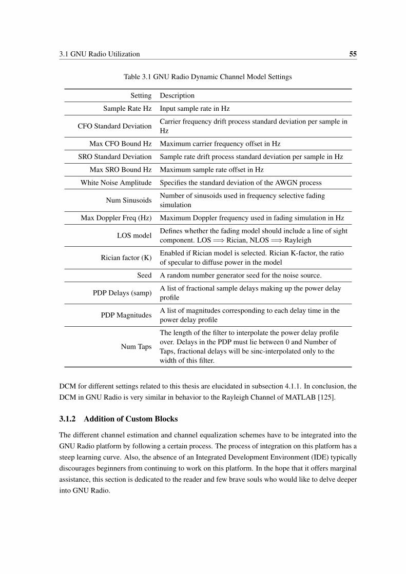
3.1 GNU Radio Utilization 55
Table 3.1 GNU Radio Dynamic Channel Model Settings
Setting Description
Sample Rate Hz Input sample rate in Hz
CFO Standard DeviationCarrier frequency drift process standard deviation per sample inHz
Max CFO Bound Hz Maximum carrier frequency offset in Hz
SRO Standard Deviation Sample rate drift process standard deviation per sample in Hz
Max SRO Bound Hz Maximum sample rate offset in Hz
White Noise Amplitude Specifies the standard deviation of the AWGN process
Num SinusoidsNumber of sinusoids used in frequency selective fadingsimulation
Max Doppler Freq (Hz) Maximum Doppler frequency used in fading simulation in Hz
LOS modelDefines whether the fading model should include a line of sightcomponent. LOS =⇒ Rician, NLOS =⇒ Rayleigh
Rician factor (K)Enabled if Rician model is selected. Rician K-factor, the ratioof specular to diffuse power in the model
Seed A random number generator seed for the noise source.
PDP Delays (samp)A list of fractional sample delays making up the power delayprofile
PDP MagnitudesA list of magnitudes corresponding to each delay time in thepower delay profile
Num Taps
The length of the filter to interpolate the power delay profileover. Delays in the PDP must lie between 0 and Number ofTaps, fractional delays will be sinc-interpolated only to thewidth of this filter.
DCM for different settings related to this thesis are elucidated in subsection 4.1.1. In conclusion, theDCM in GNU Radio is very similar in behavior to the Rayleigh Channel of MATLAB [125].
3.1.2 Addition of Custom Blocks
The different channel estimation and channel equalization schemes have to be integrated into theGNU Radio platform by following a certain process. The process of integration on this platform has asteep learning curve. Also, the absence of an Integrated Development Environment (IDE) typicallydiscourages beginners from continuing to work on this platform. In the hope that it offers marginalassistance, this section is dedicated to the reader and few brave souls who would like to delve deeperinto GNU Radio.

56 Methodology
To address the issue of IDE for GNU Radio, the CMakeLists offers a solution. The ‘Qt Creator’which is available for download at [130], enables users to open the entire project by just makinguse of the CMakeLists. There are a few files that might be used by the C++ programs that mightnot be added to the CMakeLists. Also, the files that are linked with the graphical interface GNURadio Companion (GRC) like XML, Simplified Wrapper and Interface Generator (SWIG) and Pythonfiles are not included in the project structure. Barring these flaws, the IDE provides a lot of tools forincremental development that accelerates the process.
The channel estimation and equalization schemes can be implemented as Out Of Tree (OOT)modules [131]. However, the IEEE 802.11p model offer an easier choice of developing just a C++program that incorporates the required scheme. The function declaration must contain consistentarguments over multiple schemes to enable switching between them from the GRC. After addingthe programs and integrating them into the project, the CMakeLists have to be updated to refresh theproject structure. Additionally, the ‘gr_modtool’ that is typically used for OOT modules makes alot of assumptions on what the code looks like. Therefore its use for advanced customization andspecific changes to a module is limited [131]. The method of developing a custom block is elucidatedin Appendix section A.3.
It is evident that rapid development on the GNU Radio platform is seldom achieved. Although itoffers a free open-source alternative, it becomes increasingly difficult to develop and understand analgorithm. The lack of comprehensive documentation is an inherent characteristic of most open-sourceprojects, and GNU Radio also follows in the same footsteps. However, the hardware support ofUSRP and its continued usage in many research fields [132] is promising and can surely get betterwith time. The synchronization of data between the blocks is also not clearly evident, and with its‘thread-per-block’ architecture, the flow of data in the flow-graph is not entirely transparent either.
3.2 MATLAB Simulation Platform
The MATLAB platform is optimized for solving engineering and scientific problems. The matrix-based MATLAB language is a natural way to express computational mathematics. Built-in graphicsmake it easy to visualize and gain insights from data. A vast library of pre-built toolboxes lets youget started right away with algorithms essential to your domain. The desktop environment invitesexperimentation, exploration, and discovery. These MATLAB tools and capabilities are all rigorouslytested and designed to work together [133].
The programming philosophy of the DVB-T2 CSP platform recommends adopting a wrapperfunction for each block in the transceiver chain [73]. These blocks are also organized in a hierarchicalfolder structure. This assists in associating the block to a particular part of the communication system.Adopting these design guidelines and adding multiple configuration files enables a modular structurethat can be used to mix-and-match efficiently without the need to rewrite codes. Even if the codehas to be altered to test additional algorithms, the development time, which includes writing thecode, debugging the programs, and eventually collecting results, is tremendously minimized when

3.3 Delay Dictionary 57
compared to the GNU Radio platform. Therefore, the contribution of the simulation platform as partof this thesis, is expected to be much more valuable to the research community that are dependent ondeveloping algorithms that improve efficiency of the system.
The cognitive framework and the improved matching pursuit algorithms that are introduced laterin the thesis are also implemented on the platform and is available for download at [74]. The RayleighChannel object in MATLAB has already been investigated extensively and also endorsed repeatedlyin communication system literature [75][76][77]. Addition of a custom block is as simple as writing asingle program and calling the function at the desired spot in the communication system. Furthermore,the documentation related to MATLAB is comprehensive and freely available. Additional details onthe simulation platform and it’s compatibility is given in Appendix section A.4.
3.3 Delay Dictionary
One of the elemental requirements for efficient performance of the MP algorithms is the completeand redundant dictionary, as explained in subsection 2.8.2. In this section, the construction of such adictionary is explained with respect to the delay in the channel. The dictionary aspects relating toDoppler is explained in section 3.4. In a highly mobile environment, the MP algorithm is expected toaccurately estimate the multipath delays along with the associated complex weighting factors and thecorresponding Doppler shift. In order to find the right set of dictionary columns that parameterize thechannel, it is imperative that there is a high correlation between the received signal and the correctset of dictionary columns. Thus, the construction of the dictionary should be similar to the differentperturbations exhibited by the channel.
3.3.1 The Classical Procedure
To generate the dictionary elements of the delay dictionary, we have to consider the effects of multipathdelay on the long preamble. A delay in the channel means a time shift in the time domain. If lllt ∈CN×1
is the long preamble being transmitted in the channel in the time domain, where N is the FFT length,then all the time delays can be represented by Equation 3.1, where CCC ∈ CN×N is a circular matrixcontaining coefficients as shown in Equation 3.2.
llltdelayed =CCClllt (3.1)
CCC =
c0 c1 · · · cN−2 cN−1
cN−1 c0 · · · cN−3 cN−2... cN−1 c0 c1
...
c2. . . . . . . . . c1
c1 c2 · · · cN−1 c0
(3.2)

58 Methodology
One of the important property of the circular matrix is that they are converted to a diagonal matrixby performing a Discrete Fourier Transform (DFT). The linear equations containing such matricescan be easily calculated using the FFT. It is also important to note another property of the Fouriertransform, the time shift property, which states that the Fourier transform of a time shifted signal isnothing but the Fourier transform of the primary signal multiplied by a complex exponential that isproportional to the time shift. This is represented in Equation 3.3, where G( f ) represents the Fouriertransform of g(t), and “” represents the transformation from the time domain to the frequencydomain.
g(t − tτk) e− j2π f ·tτk ·G( f ) (3.3)
These properties are exploited to create the delay dictionary of the long preamble. The longpreamble vector is given in subsection 2.2.2, which is defined in the frequency domain. Hence, wecan consider this as G( f ) in Equation 3.3. The values of f in the equation is derived from section 2.1,where centering of the OFDM symbol was also highlighted. Considering only the complex base-bandequation of OFDM, the frequency index vector fsc can be defined as Equation 3.4, where δ f representsthe sub-carrier spacing.
fsc =
([0 1 2 · · ·(N −1)
]− N
2
)· (δ f ) (3.4)
The value of Sub-Carrier Spacing is given in section 2.2, which is 156.25kHz for IEEE 802.11p.The FFT length is an even number, 64 for IEEE 802.11p, which results in N−1
2 not being an integernumber. Therefore, the centering value is chosen as N
2 to coincide with the DC frequency definedin IEEE 802.11p, which is explained in subsection 2.2.1. Now that the vector f has been defined,Equation 3.3 is just putting these values into the exponential function and multiplying it with 2π andthe delay value. Then multiply the result with the frequency domain preamble values (G( f )). Notethat the result of Equation 3.3 is a vector whose length is equal to the FFT size. This becomes asingle column of the delay dictionary matrix. By varying the value of t0, the dictionary is populated toinclude all possible expected delays in the channel. The maximum delay is determined by the cyclicprefix explained in subsection 2.2.4, which is 1.6µs for IEEE 802.11p.
The creation of dictionary represents the first step in the MP algorithm elucidated in Table 2.9.However, to give an estimate of the size of the dictionary, consider that the minimum resolution (∆τ ) ofdelay search is set to 1ns. If 1.6µs is the maximum delay that can be experienced and then corrected inthe channel, then the number of columns would be 1.6µ
1n = 1600 columns. Each column is of length 64,which is the FFT length. Then the total number of cells in the entire dictionary is 1600×64 = 102400.Each cell is a floating point complex number, which means it is typically 8 bytes. So the totalamount of memory required to store the dictionary would be 102400×8 = 819200bytes = 800kB.This is quite a large memory footprint in practical system, and therefore instead of storing the entiredictionary, the columns of the dictionary are calculated as and when they are required.

3.3 Delay Dictionary 59
The linear search for the delay involves finding the delays by progressively running the algorithmfrom zero delay to the maximum delay one after the other in steps defined by the minimum delayresolution (∆τ ). By performing the delay search independent of the Doppler, the size of the dictionaryand thus the search has already been reduced by a order of magnitude compared to the given algorithmin [22]. The second step in the algorithm, listed in Table 2.9, calculates the rank-one projectionsby multiplying the Hermitian transpose of the dictionary columns with the received long preamble.Storing the values of the rank one projections is not as demanding as storing the entire dictionary.
There are a lot of performance improvements that have been done in the code, like hard codingthe value of the ℓ2 norm of the dictionary columns, which is expected to be the same for all dictionarycolumns as the different delay values only vary the phase of the preamble and not the magnitude.Many steps in the algorithm are repeated for both the BMP and OMP, therefore it made sense tofollow a modular structure of programming, where a pool of common functions were defined andused accordingly in the different algorithms. To avoid reinventing the wheel, optimized libraries formatrix operations in C++, called as the Eigen library (Appendix section A.1), and efficient librariesfor FFT operations, called as VOLK (Appendix section A.2) were used on the GNU Radio platform.
3.3.2 The Wavelet Procedure
A multipath delay τk, according to Fourier transform theory, can be represented as a frequencydependent phase shift in the frequency domain. If lllp ∈ CN×1 represents the specified preamble inthe frequency domain as a column vector whose size N is the FFT size, and e− j2π fff ·τk represents thefrequency dependent phase shift due to the delay τk, then each column of the delay dictionary is givenby Equation 3.5, where dddp,τk ∈ CN×1 and ‘’ represents the element-wise multiplication operator.
dddp,τk = lllp e− j2π fff ·τk (3.5)
Here, fff is sub-carrier frequency index centered around the DC sub-carrier given by Equation 3.4.If K is the total number of delay bins after sampling the delay profile, the complete dictionary isdenoted as DDDτ ∈ CN×K . The complex exponential function with a precision n has a complexity ofO(2log2(n)) [134][135]. Thus, the total computational complexity associated with generating theentire dictionary is O(KN ×2log2(n)) and assuming the complex float data type, the correspondingmemory requirements is 8NK bytes. Even assuming a coarse sampling of the delay profile, thecomputational complexity and the memory requirement related to the dictionary is significant and canhinder the practical implementation on consumer hardware. Note that, with classical MP algorithms,like BMP and OMP, the resource requirements is even higher because the dictionary must also modelthe Doppler shift.
A novel method is proposed that exploits the periodicity of the delay vectors to reduce complexityand storage requirements of the delay dictionary in the frequency domain. The idea is to store a singlehigh resolution vector that contains all the possible complex values of the delay vectors. Subsequently,pointer arithmetic is employed to generate the required delay vector. The high resolution vector is

60 Methodology
labeled as the mother wavelet and is given by dddmw,Ω = e− j·ΩΩΩm . For a given delay resolution ∆τ andsampling interval Ts, ΩΩΩm is an array consisting of values from −π to +π in steps of 2π∆τ
NTsas shown in
Equation 3.6.
ΩΩΩm =−π +n ·2π∆τ
N ·Ts, n = [0,1, · · ·(NTs
∆τ
)] (3.6)
The pointer arithmetic generates the indices that extracts respective values from the motherwavelet and creates the corresponding delay vector for the particular delay τk. As the OFDM symbolsare centered, as shown in Equation 3.4, there are positive and negative frequency sub-carriers. This isanalogous to moving along the unit circle in a counter-clockwise direction for the positive frequencies,and moving in the clockwise direction for the negative frequencies. Accordingly, for each delayτk, there are two sets of indices to construct the entire delay vector. The negative frequency sub-carrier indices are given by Equation 3.7, where ααατcw ∈ ZN
2 ×1, Z represents integer numbers, andψψψ i = [0,1, · · · N
2 ].
ααατcw =NTs
2∆τ
−1− (N2· τk
∆τ
−1)+ψψψ i ·τk
∆τ
(3.7)
Similarly, the positive frequency sub-carrier indices along-with the DC sub-carrier is given byEquation 3.8, where again ααατccw ∈ ZN
2 ×1 and ψψψ i = [0,1, · · · N2 ].
ααατccw =NTs
2∆τ
+ψψψ i ·τk
∆τ
(3.8)
Simplifying and combining Equation 3.7 and Equation 3.8 results in a single set of indices whichis given by Equation 3.9, where ααατk ∈ ZN×1 and λλλ i,Ω = [−N
2 · · ·(N2 −1)]. The ‘ mod ’ represents the
modulo operation to enable repetition of the integer indices within the bounds defined by the motherwavelet dddmw,Ω.
ααατk =
(NTs
2∆τ
+λλλ i,Ωτk
∆τ
)mod
(NTs
∆τ
)(3.9)
The delay vector is then extracted from the mother wavelet using the index set ααατk as shown inEquation 3.10.
dddp,τk = lllp dddmw,Ω(ααατk) (3.10)
The accuracy and similarity of the delay vector in Equation 3.10, when compared to the vectorgiven by Equation 3.5, depends on whether the value of NTs
∆τis an integer. If the value is an integer,
which is typically the case, then there is perfect reconstruction. However, if it is not an integer then anerror of π∆τ
NTsmight occur between the two delay vectors for the same delay τk. It is important to note
that all the operations in Equation 3.9 are integer operations and can be computed efficiently. Thesize of the mother wavelet is constant for a desired delay resolution and is equal to 8×
(NTs∆τ
+1)
.In contrast, the size of the dictionary in the classical approach is proportional to the number of

3.4 Doppler Dictionary 61
delay bins K. The complexity of the proposed scheme is also reduced to O(K) since the indexfunction is invoked K times during the MP algorithm. Moreover, the mother wavelet does not add anycomplexity at the receiver since it is pre-computed and stored in memory. Thus, the proposed ‘in vivo’scheme of generating the dictionary has significant gains in both computational complexity as well asmemory requirements. Furthermore, this method is also applicable to the construction of the Dopplercomponent of the dictionary and can be used with any variant of CS based channel estimation scheme.
3.4 Doppler Dictionary
Independent search of the delay and Doppler leads to generation of separate dictionaries in thefrequency and time domain, respectively [22]. This reduces the complexity of the MP algorithm aswell as the size of the dictionary. If K represents the number of delay bins and L represents the numberof Doppler bins, then the combined delay-Doppler search would result in a dictionary having KLnumber of columns. However, an orthogonal search of delay and Doppler includes a delay dictionaryof K columns first, and then the relevant Doppler dictionary of L columns is considered. Therefore,the two separate dictionaries would have a total of K +L columns. The generation of the independentDoppler dictionary in the time domain is fairly identical to the generation of the delay dictionary. Thedifference lies in the domain that the dictionary belongs to.
3.4.1 The Classical Procedure
A Doppler shift is a frequency shift in the frequency domain, which is nothing but a complexexponential in the time domain as shown in Equation 3.11, where “” represents the transformationfrom the frequency domain to the time domain.
G( f − fd) e j2π fd ·tg(t) (3.11)
Here t becomes the Doppler index, and is given by Equation 3.12, where Ts is the sampling timeinterval.
tTs =([
0 1 2 · · ·(N −1)])
· (Ts) (3.12)
To create the columns of the Doppler dictionary, the values of t from Equation 3.12 is substitutedin Equation 3.11. By varying the value of fd for different Doppler shifts in Equation 3.11, differentcolumns of the dictionary are generated. This can be represented by Equation 3.13, where lllt ∈ CN×1
is the specified preamble in time domain.
dddp, fd = lllt e− j2π fd ·ttt (3.13)

62 Methodology
3.4.2 The Wavelet Procedure
The technique for generating the Doppler dictionary using a mother wavelet is almost identical tothe process elaborated in subsection 3.3.2. The Equation 3.13 can be modified to dddmw,θ = e− j·θθθ m
to represent the mother wavelet for the Doppler dictionary. For a given maximum Doppler offmax, Doppler resolution ∆ f and sampling interval Ts, θθθ m is an array consisting of values from 0 to2π · (N −1) ·Ts · fmax in steps of 2π ·∆ f ·Ts as shown in Equation 3.14.
θθθ m = n ·2π∆ f ·Ts, n = [0,1, · · ·((N −1)
fmax
∆ f
)] (3.14)
The pointer arithmetic generates the indices that extracts respective values from the motherwavelet and creates the corresponding Doppler vector for the particular Doppler fd . Here the indexof the samples of the OFDM symbol are linear, and there are no samples that have a negative index.Therefore, all indices start from 0 and is given by a single set of indices generated using Equation 3.15,where ααα fd ∈ ZN×1 and λλλ i,θ = [0 · · ·(N −1)].
ααα fd = λλλ i,θfd
∆ fd
(3.15)
The Doppler vector is then extracted from the mother wavelet using the index set ααα fd as shown inEquation 3.16.
dddp, fd = lllt dddmw,θ (ααα fd ) (3.16)
The simplification in generating the Doppler dictionary is due to the fact that the maximum Dopplerfmax is generally defined to be less than half of the sub-carrier spacing. Whereas the maximum delay,limited by the cyclic prefix, is a multiple of the sampling interval Ts. Another important differencebetween the two dictionaries is that a Doppler shift can be a positive or a negative shift, but timeshifts can only be delays, hence the negative range of Doppler shifts must also be considered. Thecorresponding Doppler dictionary for negative range of Doppler shifts can be constructed by changingthe mother wavelet to dddmw,θ = e+ j·θθθ m , and then performing the same calculations while inverting thesign of fd to make it positive. As before, all the operations in Equation 3.15 are integer operationsand can be computed efficiently. The size of the mother wavelet is constant for a desired fmax and ∆ f
and is equal to 8×((N −1) fmax
∆ f+1)
. In contrast, the size of the dictionary in the classical approachis proportional to the number of Doppler bins L. The complexity of the proposed scheme is alsoreduced to O(L). The MP algorithms generally assume that a dictionary is available and thereforeregard its complexity to be O(1). But, if the dictionary has to be generated at each iteration of the MPalgorithm then the complexity intensifies exponentially. Therefore, the wavelet methods of dictionarygeneration introduced in this thesis provide a substantial gain in complexity for the MP algorithms.

3.5 Matching Pursuit 63
3.5 Matching Pursuit
This section outlines the steps taken towards improving the performance and reducing the complexityof the MP algorithms. To prevent repetition in further research, minor incremental changes thatprovided minuscule advantage in performance are also highlighted. Few of these modifications werelater abandoned in favor of much more powerful algorithms. The MP algorithms developed as partof this thesis are then introduced and their complexity is investigated in comparison to the other MPalgorithms.
3.5.1 The Classical Matching Pursuit
In this thesis, the classical MP refers to the BMP and OMP algorithms elucidated in subsection 2.8.2and subsection 2.8.3, respectively. This forms the basis upon which the thesis builds upon andrecommends changes to improve performance and reduce complexity. By performing a delay andDoppler search simultaneously, the size of the dictionary inflates to KL columns in classical MP[15][20][51]. Orthogonal search of delay and Doppler reduces the combined dictionary size toK +L columns [22]. The BER performance of these methods show an adequate improvement overthe LS method under low Doppler shifts (≤ 2% normalized Doppler shift) [22], but deteriorate athigher Doppler shifts. The classical MP algorithm estimates the Doppler shift in the time domain bymatching a set of linear phase progressions with the received signal. Although the delay and Dopplersearch using the MP algorithm are mathematically identical, there is an asymmetry from a systemsperspective. The delays can be estimated accurately as they don’t induce ICI, while ISI is suppressedby a sufficiently large guard interval. But, estimating the corresponding Doppler shift pair in the timedomain provides inconsistent results. This is mainly due to the ICI which distorts the Doppler shiftsearch. Selectively equalizing delay taps increases the computational burden while searching for asingle global Doppler shift yields poor results after equalization [16].
3.5.2 Modifying the Received Vector
In a highly mobile environment, the MP algorithm is expected to accurately estimate the multipathdelays along with the associated complex weighting factors and the corresponding Doppler shift. Inorder to find the right set of dictionary columns that parameterize the channel, it is imperative thatthere is a high correlation between the received signal and the correct set of dictionary columns. Thus,the construction of the dictionary should be similar to the different perturbations exhibited by thechannel. The classical MP algorithm considers the entire received vector as the input, which containsboth amplitude as well as phase variations. Theoretically, the delays and the Doppler shifts are a phaseprogression in the frequency and the time domain respectively. Hence, any amplitude variations maydistort the outcome of the MP algorithm resulting in a wrong set of dictionary columns to represent thechannel. Consequently, a wrong channel estimate results in poor equalization performance. Moreover,

64 Methodology
building a dictionary containing all the amplitude and phase variations would be cumbersome andexponentially increase the memory requirement [16].
One of the novel ideas introduced in this thesis is to normalize the magnitude of the receivedpreamble to create the initial vector as shown in Equation 3.17, which is the input to the MP algorithmgiven in Table 2.9.
rrr0 =yyy|yyy| (3.17)
After normalizing, only the phase progression in the received vector remains. This correlates moreappropriately to the dictionary elements constructed above which are restricted to representing thevarying phase progression. Additionally, the rank-1 projections given by Equation 2.23 in Table 2.9are also free from amplitude variations by replacing Equation 2.22 in Table 2.9 with the normalizationstep shown in Equation 3.17. This modification was a logical step towards improving the performanceof the MP algorithms in finding the right set of columns from the dictionary and therefore is afundamental change in all the following experiments.
3.5.3 Tweaking the Doppler Matching Pursuit
The Doppler search, as mentioned before, is largely affected by the ICI. This prevents the orthogonalsearch of delay and Doppler from performing well at higher Doppler shifts. Finding only the multipathdelays using the preamble and equalizing them does not ensure good BER performance. Building theDoppler dictionary first involves finding the delays along with their coefficient (x) in the frequencydomain, that is achieved by the delay dictionary and the corresponding delay MP. These values arethen used to create a vector that is the weighted sum of the selected columns of the delay dictionary,where the weights are equal to the respective x values. This is represented in Equation 3.18, where qis the number of delays found in the delay search, dddsi are the selected columns of delay dictionary,and xi are the respective coefficients.
hhhτ f =q
∑i=1
xidddsi (3.18)
The hhhτ f is transferred to time domain by performing an IFFT as shown in Equation 3.19.
hhhτ f hhhτt (3.19)
To create the columns of the Doppler dictionary while incorporating the delays, g(t) is replaced byhhhτt in Equation 3.11. By varying the value of fd for different Doppler shifts in Equation 3.11, differentcolumns of the dictionary are generated. Note that the final step of multiplying the columns with thepreamble in time domain, shown in Equation 3.13, is ignored as the contribution of the preambleis already assimilated in Equation 3.18. Although the method performed marginally better than the

3.5 Matching Pursuit 65
independent search in finding the Doppler in the channel, the BER performance was adjacent to thatof LS.
The delay dictionary dddsi was altered to represent phase variations alone, and discard the con-tributions of the preamble in frequency domain as shown in Equation 3.20, which is in contrast toEquation 3.5.
dddsi = e− j2π fff ·τk (3.20)
Equation 3.18 and Equation 3.19 were then repeated and finally the resulting vector was multipliedwith the preamble in the time domain as shown in Equation 3.21 to generate different columns of theDoppler dictionary.
dddp, fd = lllt e j2π fd ·ttt hhhτt (3.21)
Although this change results in considering the contribution of the preamble once among all thedelays and Doppler, the performance was worse when compared to the previous method. Experimentswere performed using One-Tap and the LMMSE equalizers, resulting in no clear improvement in eitherof the equalization schemes. Additionally, it was found that there is a continuous phase progression inthe time domain due to Doppler on a single path as shown in Figure 3.2.
0 2 4 6 8 10 12 14
Samples ×10 4
-4
-3
-2
-1
0
1
2
3
4
Phase
Time Domain, Single Path, Doppler=500Hz
Fig. 3.2 Phase Progression in Time Domain
The continuous phase progression is unique to the time domain and is a result of the Dopplerin the channel. It is fairly linear within a single frame, and this can be exploited by modifying the

66 Methodology
equalizer to compensate this progression. The slope of the phase is calculated using the Dopplersearch performed at the time slot of the preamble, which is then extended linearly for the followingsymbols by multiplying the exponential term in either Equation 3.13 or Equation 3.21 by nN, wheren = 0,1 · · · is the index of the entire OFDM symbol following the preamble and N is the FFT size.A similar treatment to the delays in the frequency domain is not required as the OFDM symbols arealways transmitted in the respective sub-carriers, which means that fff in Equation 3.5 is consistent. Incontrast, the vector ttt in both Equation 3.13 and Equation 3.21 varies according to time for differentOFDM symbols.
The method of exploiting the phase progression did result in minor improvement of performance,but it wasn’t significant enough to advocate the increase in complexity. Further experiments revealedthe glaring deficiency in these methods, it assumes that the Doppler shift is common for all thedelay paths. This assumption resulted in finding the right Doppler shift for the most dominant path,but the same was not true for the other paths. The MP algorithm could then be modified to findthe corresponding Doppler shifts for each delay paths while incorporating the phase progressionindividually. However, such a method will be analogous to the classical MP algorithm and thereforeexhibit high complexity. As a solution, the following Rake Matching Pursuit algorithm was developedthat builds upon the ideas outlined in this section and still manages to offer favorable performance atmuch lower complexity.
3.5.4 Rake Matching Pursuit
The RMP algorithm utilizes the novel delay search metric that is independent of amplitude variations.This ensures the robust estimation of the multipath delays even under difficult channel conditions. Inaddition to this, an implicit estimation of the Doppler shift is proposed by tracking the variation of thetap coefficients for each of the delay taps in the frequency domain itself. The RMP algorithm and itssuperior performance, even under high Doppler shifts, has already been peer reviewed and acceptedin a paper [16].
The delay search component of the RMP is presented in Table 3.2. The rank-1 projectionsare given by Equation 3.23 which are free from amplitude variations due to the normalization inEquation 3.22. This helps in finding the right delays in the channel. The MP algorithm begins byinitializing the residual error rrr0 to the normalized received signal yyy. The received signal is projectedonto every column of the dictionary in Equation 3.23. In Equation 3.24, the projections are maximized.The coefficient of the spreading function is computed in Equation 3.26. The projections are thenupdated in Equation 3.27 by subtracting the contributions of the previous column dddsp that maximizedthe projection. The algorithm iterates until a stopping criteria is reached or the maximum number ofiterations are completed. The outcome is an estimate of the multipath delays and the associated tapcoefficients. There are many subtle changes in the algorithm that improve the overall performanceand reduce the complexity. In Equation 3.23, there is no consideration of the Doppler dictionary,and is restricted to delay dictionary. This reduces the overall burden from O(KL) to just O(K).

3.5 Matching Pursuit 67
Table 3.2 RMP Delay Search Algorithm
Initialization
rrr0 =yyy|yyy| (3.22)
b0, j = dddHj rrr0, for j = 1 · · ·K (3.23)
s1 = arg maxj=1···K
|b0, j|2∥ddd j∥2
(3.24)
iii1 = s1 (3.25)
x1 =b0,s1
∥ddds1∥22
(3.26)
b1, j = b0, j − x1dddHj ddds1 , for j = 1 · · ·K, j /∈ iii1 (3.27)
the pth iteration, p > 1
sp = arg maxj=1···K, j/∈iiip−1
|bp−1, j|2∥ddd j∥2
(3.28)
iiip = iiip−1,sp (3.29)
xp =bp−1,sp
∥dddsp∥22
(3.30)
bp, j = bp−1, j − xpdddHj dddsp , for j = 1 · · ·K, j /∈ iiip (3.31)
The advantage is even greater when the wavelet procedure for generation of the delay dictionary isemployed. Equation 3.24, Equation 3.27, Equation 3.28 and Equation 3.31 also gain by limiting thesearch to finding multipath delays. Once the dominant taps of the channel, or the multipath delays, arefound using the RMP delay search, the next step is to compensate the Doppler effect in the channel.
Once the delay paths have been recognized using the preamble. The next step is to track thevariation of the complex weighting factor with respect to the particular delay paths by performing asubset of the RMP algorithm. The Doppler, that is in the channel, implicitly results in variation of themagnitude and phase of these complex weighting factors. To track the changes of the complex weight-ing factors, the pilots in each OFDM symbol is used. Let q be the number of delay paths that havebeen found by the RMP algorithm for the preamble. Their respective delay vectors, in the frequencydomain, can be denoted as ddd1 = e j2π fff τ1 ,ddd2 = e j2π fff τ2 , · · ·dddq = e j2π fff τq . The dictionary for tracking theDoppler shift is a collection of these delay vectors represented as DDDp = [ddd1,ddd2,,, · · ·dddq]; DDDp ∈ CNp×q.

68 Methodology
The complex weighting factors found by the RMP algorithm for each of the delay paths are representedas xd1 , xd2 , · · · xdq . Let rrr ∈ C1×N be the received vector corresponding to the received OFDM symbol.rrrp contains the received symbols corresponding to the pilot sub-carriers. rrrp ∈ C1×4 is of length 4as there are only 4 pilot sub-carriers defined by the IEEE 802.11p standard. However, these pilotsare set to initial values of pppi = [1,1,1,−1], which are then influenced by a PN sequence given insubsection 2.2.3 pn ∈ −1,1. The PN sequence picks a single value within the set −1,1 and thenmultiplies all the pilots. The initial vector therefore is constructed by removing the additional phasevariations introduced by the standard and is given by rrr0 = rrrp · pppi pn. It is important to note that thenormalization of the initial vector is not performed here as the accuracy of the complex weightingfactors are under consideration. The RMP algorithm to implicitly estimate the Doppler shift is givenin Table 3.3.
Table 3.3 RMP Implicit Doppler Estimation
Initialization, DDDp ≜ [ddd1 · · ·dddq]
rrr0 = rrrppp (3.32)
b0, j = dddHj rrr0, for j = 1 · · ·q (3.33)
iii1 = 1 (3.34)
x1,rp =b0,1
∥ddd1∥22
(3.35)
b1, j = b0, j − x1,rpdddHj ddd1, for j = 1 · · ·q, j /∈ iii1 (3.36)
the pth iteration, p > 1 and p ≤ q
iiip = iiip−1, p (3.37)
xp,rp =bp−1,p
∥dddp∥22
(3.38)
bp, j = bp−1, j − xp,rpdddHj dddp, for j = 1 · · ·q, j /∈ iiip (3.39)
Find the rank-one projections of the dictionary DDDp using Equation 3.33. The rank-one projectionsare given by bbb0, j = DDDH
p rrr0, where j represents the different delay paths, which means the dimensionsare bbb0, j ∈ Cq×1. The maximization step of the RMP algorithm, Equation 3.24, is ignored as thedominant channel taps have already been found using the preamble and are sorted according totheir strengths. The next step is to find the new complex weighting factor for first delay path usingEquation 3.35. Then update the rank-one projections of all the other delay paths using Equation 3.36,other than the first delay path. For the second delay path onwards, use the previously updated rank-one

3.5 Matching Pursuit 69
projection values to find the complex weighting factors as shown in Equation 3.38. After findingthe complex weighting factor for each delay path, update the rank-one projection values again forall the other paths as shown in Equation 3.39. The algorithm stops when all the delay taps have anupdated complex weighting factor. The outcome is the updated complex weighting factors for each ofthe delay taps and thus, the complete channel information is available for every OFDM symbol thatincludes the contributions from the multipath delays as well as the Doppler shift.
Once the updated coefficients are obtained, the one tap equalizer channel matrix is constructedwhich is just the summation of delay vectors multiplied by their respective coefficients hhh f =
∑qi=1 xdinewdddi. The One Tap equalizer matrix hhh f is now used to just divide the entire received OFDM
symbol to gather the equalized symbols sss = rrrhhh f
, where sss is the equalized vector. A Doppler shiftin the channel is a temporal progression of the complex weighting factors. In scenarios of lowmobility, these factors remain constant; while with high mobility, the complex weighting factors varycontinuously within the physical layer frame. Consequently, tracking the complex weighting factorsis an implicit method to estimate the Doppler shift. Moreover, since these factors are tracked for eachof the identified delay taps, an implicit separation between the delays and the associated Dopplershift is achieved. In addition to this, such a scheme can cope with shorter coherence times (or higherDoppler shifts) since the weighting factors are tracked for every OFDM symbol. Furthermore, thecomputational burden of tracking the progression of the weighting factors is lower than conducting afull Doppler search for every delay tap in the time domain.
The complexity of the MP algorithm has been reduced considerably as there is no need toperform a Doppler search for the preambles in the RMP. Due to an independent search of delay andDoppler, the complexity, in the worst case, was brought down to O((K +L)qN) [22], where K and Lcorresponds to the delay and Doppler bins, q is the number of iterations and N is the FFT size. Withthe RMP, the complexity for delay estimation has been reduced to O(KqN) and the complexity totrack the complex weighting factors pertaining to the q estimated delays is O(qNp), where Np is thenumber of pilots.
The RMP includes a novel metric to search for the delays that is free from any amplitude variationscaused by the channel. Additionally, it also contains a novel scheme to implicitly estimate and equalizethe Doppler shift by tracking the variations of the complex weighting factors for the OFDM datasymbols. Results have shown that the channel transfer function obtained from the RMP is close to thePerfect Channel State Information (PCSI) for rapidly varying channels. An accurate channel estimatewill help overcoming the effects of a doubly selective channel. Also, the complexity of the RMP islower than that of the classical MP algorithm.
3.5.5 Gradient Rake Matching Pursuit
After multiple simulation runs and experiments, another advantage of the RMP was discovered. Itwas found that the RMP is relatively immune to errors even if wrong delay taps, in addition to theaccurate delays, are found during search. This is due to the fact that, during the tracking phase of the

70 Methodology
RMP, the magnitude of tap coefficients have a higher probability to be negligible for the wrong delaytaps. This contracts any erroneous contributions, which also minimizes the burden on the stoppingcriterion to find the exact number of delays. Consequently, the difference in RMP performancebetween finding the exact delay taps, and finding few wrong delay taps in addition to the exact delaytaps, is insignificant. But, finding lesser delay taps than the exact delays inflates the errors, resultingin significant reduction in BER performance. In this section, inherent ability of the RMP to favorover-determining the system is exploited to further reduce the complexity of the algorithm.
The Gradient Rake Matching Pursuit (GRMP) algorithm is introduced in this thesis and has alsobeen submitted as a paper which is currently under review as of the writing of this thesis. It is designedto significantly reduce the computational complexity of the channel estimation process by optimizingthe delay search. The underlying idea is to compute an imperfect estimate of the delays insteadof iteratively finding the precise delays along with the complex tap coefficients. This is motivateddue to the fact that, the rank-1 projections obtained from the delay search provides a crisp maximathat correspond to the delay taps. These crisp maxima points are characterized by monotonicallyincreasing edges that are immediately followed by decreasing edges. Thus, a gradient method isdesigned to identify these peaks and is accordingly called as the Gradient Rake Matching Pursuitalgorithm. Moreover, the implicit Doppler estimation technique is immune to inaccurately estimateddelay taps, similar to the RMP. The GRMP algorithm for the delay search is given in Table 3.4.
Table 3.4 GRMP Delay Search
Initialization
rrr0 =yyy|yyy| (3.40)
b0, j = dddHj rrr0, for j = 1 · · ·K (3.41)
s0, j =|b0, j|2∥ddd j∥2
, for j = 1 · · ·K (3.42)
m0, j = ∇sss0, sss0 = [s0, j]∀( j = 1 · · ·K) (3.43)
for j ∈ 1,2 · · ·K doif m0, j−1 ≤ m0, j ≥ m0, j+1
iii0 = iii0, j (3.44)end if
end for
xxxi0 =[DDDH
i0 DDDi0]−1 DDDH
i0 yyy (3.45)
In Equation 3.40, the error vector is initialized to the magnitude normalized received signal. Therank-1 projections corresponding to the delays are computed in Equation 3.41 and Equation 3.42. A

3.5 Matching Pursuit 71
first order derivative is computed in Equation 3.43, which is followed by identifying the most dominanttaps using a simple 1-D peak finding method given in Equation 3.44. The complex tap coefficientscorresponding to these peaks are computed in Equation 3.45. The result is a rough estimate of thedelay taps that is followed by the implicit Doppler shift estimation technique. The GRMP algorithmcircumvents the iterative ℓ1 minimization process for the delay search since an acceptable estimate isachieved by gathering the peaks of the delay rank-1 projections.
The omission of an iterative process, although greatly reduces the complexity, has slight disadvan-tages. In the iterative process, the contribution of each delay vector on the other delays is compensatedbefore every search. Even if the delay vectors are not perfectly accurate, the process still achievessimilar results to ℓ1 minimization [19][40][43]. However, this is not the case in the GRMP, there is agreater obligation for the delay vectors to be accurate in representing the multipath effects to achievefavorable performance. Additionally, the standardized channel models define an echo profile limitingthe maximum sparsity of a channel, which can be exploited to limit the gradient search to obtain onlythe required number of dominant channel taps to further reduce the complexity. The absence of aniterative process to find the dominant taps is evident from Table 3.4, which reduces the complexity toO(KN). The reduction in complexity is of the order of q, which was the number of iterations that theRMP had to perform in the delay search. However, the implicit Doppler estimation complexity of theRMP is retained by the GRMP, and is given as O(qNp), where Np is the number of pilots.
The computational complexity is progressively reduced by implementing the proposals for thedictionary and the MP algorithms. The wavelet based dictionary generation technique has minimizedthe complexity from O(KN +2log2(n)) to O(K). In addition to this, it is also shown that the memoryrequirement is also smaller when compared to the classical method to generate the dictionary. Thesearch complexity of the classical MP algorithm is in the order of O(KLqN), where q representsthe number of iteration and K&L are the total number of delay and Doppler bins respectively. Byperforming an orthogonal search of the delays and Doppler shifts, the complexity was reduced toO((K +L)qN) in [22]. The BER performance of this method shows a distinct improvement overthe LS method for low Doppler shifts (≤ 2% normalized Doppler shift), but deteriorates at higherDoppler shifts.
Contrarily, the RMP performs an implicit Doppler shift estimation that has a complexity ofO(qNp), where Np is the number of pilots in an OFDM data symbol. Additionally, the complexity ofthe delay search is O(KqN) and the overall complexity of the RMP algorithm is smaller than that ofthe classical MP algorithm. Furthermore, the RMP algorithm is shown to achieve a considerable gainin performance even at high Doppler shifts [16]. The GRMP algorithm further reduces the complexityassociated with the delay search to O(KN). However, the reduction in complexity comes with a smallpenalty in performance when compared to the RMP. But, when compared to the classical MP as wellas the LS estimation scheme, the gain in performance is significant. Furthermore, a deterministicbound on the execution time can also be calculated for the entire GRMP algorithm. However, dueto the iterative nature of the RMP and the classical MP algorithm such a bound is not available atthe receiver. The reduction in computational and memory requirements is a significant step towards
72 Methodology
the practical implementation of effective channel estimation schemes like the GRMP algorithm andenabling high mobility in consumer wireless communication systems.
3.6 The Cognitive Framework
High mobility in vehicular communication systems results in a time-varying multipath or a doublyselective channel. Such channels exhibit selectivity in both the time as well as the frequency domain.The estimation of the channel parameters plays a vital role in overcoming the effects of high mobilityat the receiver. Moreover, it is known that the estimation of a such a channel is a non-trivial task. TheMP algorithm is a CS scheme that works well in scenarios of high mobility. However, it is shown thatunder less severe channel conditions, simpler channel estimation and equalization schemes can bemore power-efficient and hence increase battery-life without reducing the quality of the equalization.In this thesis, a cognitive framework is proposed that optimizes the estimation scheme based onthe channel conditions and certain measurements from the receiver chain. The result is a channelestimation scheme that is robust, precise and reliable in all channel conditions while adapting thecomplexity to be optimal for the channel being estimated.
Current techniques for the estimation of a doubly selective channel make a trade-off betweencomplexity and performance. Moreover, an ideal channel estimator is also desired to work witha lower complexity in scenarios of low mobility. Schemes such as the RMP algorithm provide arobust and accurate estimate of a doubly selective channel. However, in scenarios of low mobility, thecomplexity associated with the RMP algorithm is prohibitive and the use of conventional schemessuch as the LS channel estimator is more appropriate. Therefore a cognitive framework is proposedthat ensures robust performance with the least complexity subject to channel conditions. In thisthesis, a novel cognitive framework is proposed that switches between the RMP scheme for channelestimation and the LS channel estimator based on different metrics derived from the receiver. It willbe shown that the proposed cognitive framework not only switches between the two schemes forchannel estimation but also chooses the least complex scheme depending on channel conditions.
The incentive to develop a cognitive framework stems from the fact that different channel estima-tion methods do not offer reliable performance at optimum complexity under all channel conditions.Illustrating this clearly is the LS scheme, whose performance at minimal complexity is notable butrestricted to low mobility environments. Contrarily, the RMP performance is far superior under highmobility environments but at the cost of greater complexity. But, under low mobility conditionsRMP performs relatively close to the LS [16], and hence its use becomes unnaturally excessive. Aframework that can detect the different channel conditions, and not necessarily estimate them, ata marginal increase in complexity will facilitate the switch between different channel estimationmethods to consistently provide good performance at optimum complexity.
An ideal cognitive framework, depending on the channel conditions, would choose the channelestimation method that offers the best performance at the lowest complexity for every OFDM symbol.The metrics for detecting the channel conditions should also add minimal complexity, which is O(1)
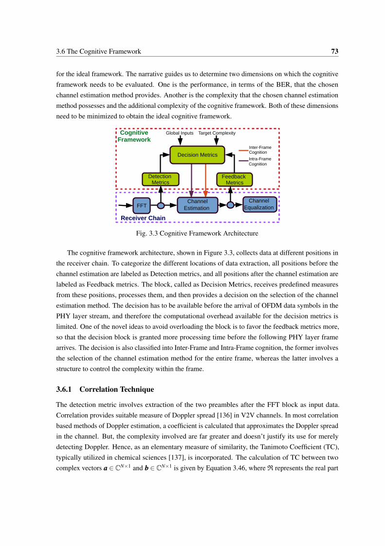
3.6 The Cognitive Framework 73
for the ideal framework. The narrative guides us to determine two dimensions on which the cognitiveframework needs to be evaluated. One is the performance, in terms of the BER, that the chosenchannel estimation method provides. Another is the complexity that the chosen channel estimationmethod possesses and the additional complexity of the cognitive framework. Both of these dimensionsneed to be minimized to obtain the ideal cognitive framework.
Fig. 3.3 Cognitive Framework Architecture
The cognitive framework architecture, shown in Figure 3.3, collects data at different positions inthe receiver chain. To categorize the different locations of data extraction, all positions before thechannel estimation are labeled as Detection metrics, and all positions after the channel estimation arelabeled as Feedback metrics. The block, called as Decision Metrics, receives predefined measuresfrom these positions, processes them, and then provides a decision on the selection of the channelestimation method. The decision has to be available before the arrival of OFDM data symbols in thePHY layer stream, and therefore the computational overhead available for the decision metrics islimited. One of the novel ideas to avoid overloading the block is to favor the feedback metrics more,so that the decision block is granted more processing time before the following PHY layer framearrives. The decision is also classified into Inter-Frame and Intra-Frame cognition, the former involvesthe selection of the channel estimation method for the entire frame, whereas the latter involves astructure to control the complexity within the frame.
3.6.1 Correlation Technique
The detection metric involves extraction of the two preambles after the FFT block as input data.Correlation provides suitable measure of Doppler spread [136] in V2V channels. In most correlationbased methods of Doppler estimation, a coefficient is calculated that approximates the Doppler spreadin the channel. But, the complexity involved are far greater and doesn’t justify its use for merelydetecting Doppler. Hence, as an elementary measure of similarity, the Tanimoto Coefficient (TC),typically utilized in chemical sciences [137], is incorporated. The calculation of TC between twocomplex vectors aaa ∈ CN×1 and bbb ∈ CN×1 is given by Equation 3.46, where R represents the real part

74 Methodology
Fig. 3.4 Correlation based Decision Metric Flowchart
of a complex number. Coincidentally, the TC has a value of ‘1’ if the two preambles are perfectlycorrelated, and its value approaches ‘0’ for uncorrelated preambles.
TC (aaa,bbb) =R(aaaH ·bbb)
∥aaa∥22 +∥bbb∥2
2 −R(aaaH ·bbb)(3.46)
For cognition in the correlation based cognitive framework, the following metrics are adopted.
• Intra-Frame Preamble TC is computed for the two received preambles of a PHY frame andworks well under high mobility.
• Inter-Frame Preamble TC is the averaged TC between the preambles of consecutive framesand works well for moderate Doppler shifts.
• Inter-Frame Chan TC quantifies the similarity between the channel transfer function hhh f ofconsecutive frames.
3.6 The Cognitive Framework 75
• xxx-variance quantifies the temporal variation of the tap coefficients x in a given frame, which iscalculated in RMP using Equation 3.38 of Table 3.3.
All the benchmarks from the detection metrics and feedback metrics are forwarded to the decisionmetrics block, where a priority scheme has been established to create a hierarchical structure based onthe level of confidence of each input metric. The priority scheme is represented by a flowchart shownin Figure 3.4. The scheme mainly has two branches, one branch is concerned with the low mobilitymethod like LS, another with the high mobility method like RMP. The input metrics, along withthe decision scheme, indicate whether the system has to continue with the previously used channelestimation method or switch to another. However, for the first frame, the detection metric ‘Intra-FramePreamble TC’ alone chooses between the different channel estimation methods. The outcome of thiscognitive framework is an optimized channel estimation scheme which provides the best estimateof the channel parameters with the least complexity. The channel transfer function computed fromthe channel parameters is used to construct a one-tap equalizer which compensates the effects of thechannel.
The computational complexity for LS considering the two preambles of the entire PHY layerframe is O(2N), where N is the FFT size. However, the computational complexity of the RMP forfinding the channel taps using the preamble is O(KqN), where K corresponds to the number of delaybins, and q is the number of iterations. Additionally, tracking the tap coefficients in an OFDM symbolhas a complexity of O(qNp), where Np represents the number of data pilots. Combining both, theoverall complexity of RMP for an entire PHY layer frame is O(KqN +SqNp), where S is the numberof OFDM data symbols in the frame. For a typical multipath environment, q < 6 and K ≈ 50 for adelay search resolution of 10ns or less. This cognitive framework, on the other hand, has two TCsbeing calculated with the complexity of O(N), and the averaged TC with a complexity of O(2N). Italso calculates the variation of x values with O(q) complexity when the RMP is selected. Therefore,the additional complexity of the cognitive framework for an entire PHY layer frame is O(4N +q).Thus, in contrasting channel conditions, this cognitive framework provides a considerable reductionin complexity.
The thresholds set for the TC is dependent on the SNR, and therefore is susceptible to errors.Multiple simulations were performed under different SNR levels and varying Doppler. The datacollected from them showed that the TC followed an exponential curve for different SNR levels.Furthermore, the values gradually reduced and approached zero as the Doppler shift in the channel wasincreased. Collecting the values at lower Doppler and finding a least squares fit with an exponentialfunction resulted in Equation 3.47, where γTC is the threshold calculated according to the SNR. Theprogram used to find the least squares fit in MATLAB is given in Appendix section A.5 for reference.
γTC =−0.9 · e−0.14·SNRdB +1 (3.47)
In contrast, the xxx-variance threshold is more robust to noise. The xxx values for multiple paths overdifferent SNR and varying Doppler was collected in a huge data set. It was found that the variation

76 Methodology
of both the real part and the imaginary part of the complex coefficient was below ‘0.11’ under lowDoppler shifts. If xxxt0 represents the complex coefficients of the first OFDM data symbol and xxxtn
represents the complex coefficients for the last OFDM data symbol in the entire frame. Then thexxx-variance can be calculated using Equation 3.48, where xxxσ2,R and xxxσ2,I represent the variation of thereal part and the imaginary part of the complex coefficient respectively, and I is the imaginary partsof complex numbers in the complex vector.
xxxσ2,R = |R(xxxtn)−R(xxxt0)|xxxσ2,I = |I(xxxtn)−I(xxxt0)|
(3.48)
The above values are then compared with the xxx-variance threshold given by Equation 3.49.
γxxx = 0.11 (3.49)
The structure of the preambles in the frequency domain can be exploited to calculate the SNR atthe receiver. The received power is given by Equation 3.50, where yyyL,n represents all the non-zerosub-carriers of the received preamble in the frequency domain. The fraction 1
52 is added as there are52 non-zero sub-carriers in IEEE 802.11p.
PR =1
52
(∑∣∣yyyL,n
∣∣2) (3.50)
Exploiting the zero sub-carriers, the noise power can also be calculated using Equation 3.51,where yyyL,0 contains the values of received vector in the frequency domain at those positions where thesub-carriers are set to zero. The fraction 1
12 is added as there are 12 sub-carriers in IEEE 802.11p thatare set to zero.
PN =112
(∑∣∣yyyL,0
∣∣2) (3.51)
The SNR is then calculated using Equation 3.52.
SNRdB = 10 · log10
(PR −PN
PN
)(3.52)
Although the adoption of the TC as a measure of correlation to detect Doppler was not misplaced,its threshold sensitivity to SNR creates a learning phase for the cognitive framework that can beundesirable in practical systems. Additionally, the SNR calculation method described above is alsoprone to errors. Even with these limitations the correlation based cognitive framework still performsremarkably well in most channel conditions.
3.6.2 Complex Coefficient Technique
In the correlation based cognitive framework, the TC suffers from noise variations which result insubnormal performance of the cognitive framework under very low SNR conditions. The metrics
3.6 The Cognitive Framework 77
strive to choose the right scheme, but falls short of perfection. Additionally, the calculation of threeTCs adds marginal complexity. To improve the performance, while minimizing the complexity,the complex coefficient based cognitive framework is designed exploiting the knowledge that thexxx-variance is more robust to noise. The architecture of the cognitive framework remains the same asshown in Figure 3.3.
The complex coefficient is x which quantifies the temporal variation of the tap coefficients and iscalculated in RMP using Equation 3.38 of Table 3.3. The same is carried over to this framework also,but such temporal variation is unavailable when LS scheme is chosen. To solve this problem, the delayvalue of the most dominant tap of the RMP is stored as one of the feedback metric. This suggeststhat the RMP must be executed at-least once before the LS scheme is chosen. Therefore, the globaldefault is set to RMP, and if there was no previous decision that was made, then the RMP schemeis chosen by default. Once the dominant delay path τ0 is known, then the corresponding complexcoefficient can be calculated for each preamble by Equation 3.53, where dddτ0 ∈ CN×1 is calculatedusing Equation 3.5, and yyyL ∈ CN×1 can be either of the two preambles.
xLS =dddH
τ0· yyyL
∥dddτ0∥22
(3.53)
The complex coefficient can also be calculated for each of the two preambles and their variationsaveraged between frames to provide a much more balanced view of its variation. The xLS is there-fore named as the ‘Dominant Tap x-variance’, as it tracks the variation of the complex coefficientcorresponding to the most dominant path between preambles of consecutive frames. Combining thexxx-variance from above subsection 3.6.1, and the xLS simplifies the decision metric to a great extent asshown in Figure 3.5.
The computation of SNR that is performed in Equation 3.52 is no longer required, as the thresholdγxxx given by Equation 3.49 is constant for all SNR and all Doppler shifts. The additional complexityof calculating xLS is O(N), and the complexity involved with xxx-variance remains the same at O(q).Combining them, the overall additional complexity of the complex coefficient based cognitiveframework for the entire frame is reduced to just O(N + q). The performance of this cognitiveframework is also superior at lower SNRs due to the metrics being more robust to noise.

78 Methodology
Fig. 3.5 Complex Coefficient based Decision Metric Flowchart

Truth, also is the pursuit of it.
George Oppen
Part IV
The Climax
79


CHAPTER 4RESULTS
Supported by all the nuts and bolts of the previous chapter, it is finally time to take the platforms fora test drive. This chapter provides more details of the platform on which the tests were performed.The method followed to generate the results are also explained. Interpretation of the results are alsoexamined to provide confidence in the chosen path.
4.1 GNU Radio Test Bed
Few changes were made to the IEEE 802.11p model in GNU Radio that was introduced in subsec-tion 2.5.1. The “IEEE 802.11p Software Loopback” (Figure 2.9) was changed to include the DCMexplained in subsection 3.1.1. The flow-graph containing the changes is shown in Figure 4.1. Theinput to the flow-graph is modified so that the messages are transmitted for a defined duration. Thisensures better consistency over multiple simulations. The following block “WiFi MAC” is modifiedinternally to generate a consistent block of messages that include the MAC header, parity bits, andCyclic Redundancy Check (CRC) field. This modification is required for template matching of thebits to calculate the BER. Additional graphical sinks have been disabled to reduce unnecessary loadon the computer.
The PHY Hierarchical flow-graph that was shown in Figure 2.10 has also been altered to enablelogging and debugging points. Along with these type of modifications, internally the different channelestimation and channel equalization schemes have also been added, and these can be selected fromthe main flow-graph. The “WiFi mapper” from the earlier hierarchical flow-graph has been changedto avoid randomizing the data by disabling scrambling, convolutional encoding and puncturing of theincoming symbols. The data at this juncture in packed into the PMT containers and sent through thenewly created output port. These modifications are to generate a well defined template that is repeatedin every frame, so that the BER calculations at the receiver can be performed by a simple templatematching process. Logging of the transmitted data is also added in this block.
Similarly on the receiver side, the “WiFi Decode MAC” has been changed to log the receiveddata before deinterleaving and before any of the convolutional decoding is performed. This isdone to remove any gain due to convolutional decoding in the BER calculations. The logged data

82 Results
Fig. 4.1 Software Loopback with DCM
in the transmitter, as mentioned before, is after scrambling, convolutional coding, puncturing andinterleaving in transmit chain. But among them, scrambling is disabled to prevent any change indata, convolutional coding is performed as the input stream is always consistent which results inthe output of the convolutional coder being constant for each frame. Puncturing and interleavingis also not varied for the entire simulation to generate a well defined constant transmit stream. Itshould be noted that these steps just change the data in a predefined manner and are not actuallycontributing to any gain in BER performance by themselves. Only when they are combined withinverse blocks in the receiver, the gain in BER performance is achieved. To exemplify this more,consider convolutional encoding, it just represents the incoming byte stream in another set of bytes.Only when the convolutional decoding in the receiver is exploited, the gain in BER performance dueto convolutional coding is achieved. The files are logged at the debug points in the transmitter andreceiver chains. These files are stored and later, in offline analysis using MATLAB, they are read-outto generate the respective plots.
4.1.1 Dynamic Channel Model Evaluation
The dynamic channel model, annotated in subsection 3.1.1, was evaluated to check whether thedesired channel behavior was being generated. The long preamble was stored in a binary file andthen analyzed in MATLAB to generate the plots shown in this section. The DCM settings for thedifferent test cases are shown in Figure 4.2. The DCM settings have been explained in Table 3.1 insubsection 3.1.1.

4.1 GNU Radio Test Bed 83
(a) No delay, No Doppler (b) Low delay, No Doppler
(c) High delay, No Doppler (d) No delay, Low Doppler
(e) No delay, High Doppler (f) High delay, High Doppler
Fig. 4.2 DCM Settings for evaluation

84 Results
The sample rate offset and frequency offset have been consistently set to zero in all the test cases,as they are mainly used to simulate the crystal oscillator behavior in communication hardware. Themajor focus of this thesis are the channel effects on the signal, hence these settings of the DCMhave been ignored. The method used for offline analysis in MATLAB was simply normalize theamplitude of the received long preamble. Then divide the received long preamble with the knownpreamble for all the non-zero sub-carriers to get the frequency domain response of the channel. Forthe time domain response, the same amplitude normalization was performed, and then the IFFT ofthis normalized received vector was performed. IFFT also introduces a normalization factor of 1
N , thisis important when considering the division of the received vector by the IFFT of the long preamble. Ifthe normalization factors are the same for both the received vector and the long preamble, then thedivision of the IFFT of received vector with the IFFT of the known preamble is valid. The magnitudeand phase after this division is plotted as the time domain response of the channel.
No delay, No Doppler
One of the first test was to check whether the channel produced any undesired effects when the settingswere set to zero delay and zero Doppler. The DCM settings are shown in Figure 4.2a. The frequencydomain and time domain response of the channel is shown in Figure 4.3a. As expected, the variationin phase and amplitude is negligible and almost a straight line. However, there is an initial phase shiftand non-unity gain in the channel.
Phase changes due to delay
The next test was to check the channel response under a high delay condition. Note that the settingsshown in Figure 4.2c, simulate two paths, one with no delay and another with 14 sample delay. Ifonly a single path of 14 samples were generated, then the synchronization block in the receiver wouldcompensate for this delay and the receiver would perceive it as a “No Delay” condition. The channelresponse is shown in Figure 4.3b. Our interest is the variation of phase in the frequency domain, asdelay in time domain corresponds to phase in the frequency domain. The response of the channel is asexpected, the phase variation is high when the signal passes through a high delay channel. Comparethis with the low delay channel response shown in Figure 4.3c, the variation of phase is much slowerin the frequency domain under low delay conditions. The DCM settings for the low delay and noDoppler condition is shown in Figure 4.2b. In conclusion, the DCM is satisfactorily simulating thedelay according to the conventional norms.
Phase changes due to Doppler
Once it has been established that the delay is being simulated according to the expected behavior,the next logical step is to observe the changes to the signal due to Doppler. The DCM settings forlow Doppler and high Doppler are shown in Figure 4.2d and Figure 4.2e respectively. The channelresponse for these settings are shown in Figure 4.3d and Figure 4.3e respectively. As expected, the
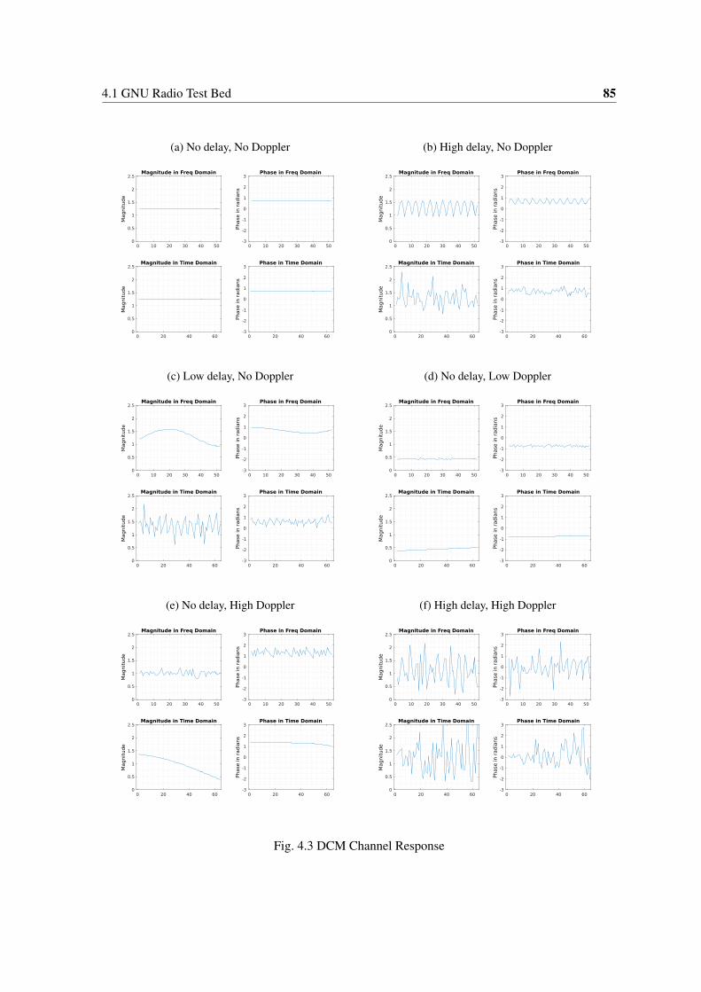
4.1 GNU Radio Test Bed 85
(a) No delay, No Doppler
0 10 20 30 40 500
0.5
1
1.5
2
2.5
Magnit
ude
Magnitude in Freq Domain
0 10 20 30 40 50-3
-2
-1
0
1
2
3
Phase
in r
adia
ns
Phase in Freq Domain
0 20 40 600
0.5
1
1.5
2
2.5
Magnit
ude
Magnitude in Time Domain
0 20 40 60-3
-2
-1
0
1
2
3
Phase
in r
adia
ns
Phase in Time Domain
(b) High delay, No Doppler
0 10 20 30 40 500
0.5
1
1.5
2
2.5
Magnit
ude
Magnitude in Freq Domain
0 10 20 30 40 50-3
-2
-1
0
1
2
3
Phase
in r
adia
ns
Phase in Freq Domain
0 20 40 600
0.5
1
1.5
2
2.5
Magnit
ude
Magnitude in Time Domain
0 20 40 60-3
-2
-1
0
1
2
3
Phase
in r
adia
ns
Phase in Time Domain
(c) Low delay, No Doppler
0 10 20 30 40 500
0.5
1
1.5
2
2.5
Magnit
ude
Magnitude in Freq Domain
0 10 20 30 40 50-3
-2
-1
0
1
2
3
Phase
in r
adia
ns
Phase in Freq Domain
0 20 40 600
0.5
1
1.5
2
2.5
Magnit
ude
Magnitude in Time Domain
0 20 40 60-3
-2
-1
0
1
2
3
Phase
in r
adia
ns
Phase in Time Domain
(d) No delay, Low Doppler
0 10 20 30 40 500
0.5
1
1.5
2
2.5
Magnit
ude
Magnitude in Freq Domain
0 10 20 30 40 50-3
-2
-1
0
1
2
3
Phase
in r
adia
ns
Phase in Freq Domain
0 20 40 600
0.5
1
1.5
2
2.5
Magnit
ude
Magnitude in Time Domain
0 20 40 60-3
-2
-1
0
1
2
3Phase
in r
adia
ns
Phase in Time Domain
(e) No delay, High Doppler
0 10 20 30 40 500
0.5
1
1.5
2
2.5
Magnit
ude
Magnitude in Freq Domain
0 10 20 30 40 50-3
-2
-1
0
1
2
3
Phase
in r
adia
ns
Phase in Freq Domain
0 20 40 600
0.5
1
1.5
2
2.5
Magnit
ude
Magnitude in Time Domain
0 20 40 60-3
-2
-1
0
1
2
3
Phase
in r
adia
ns
Phase in Time Domain
(f) High delay, High Doppler
0 10 20 30 40 500
0.5
1
1.5
2
2.5
Magnit
ude
Magnitude in Freq Domain
0 10 20 30 40 50-3
-2
-1
0
1
2
3
Phase
in r
adia
ns
Phase in Freq Domain
0 20 40 600
0.5
1
1.5
2
2.5
Magnit
ude
Magnitude in Time Domain
0 20 40 60-3
-2
-1
0
1
2
3
Phase
in r
adia
ns
Phase in Time Domain
Fig. 4.3 DCM Channel Response

86 Results
phase variation in the time domain is higher under the high Doppler condition compared to the lowDoppler condition. However, it must be noted that the Doppler setting in the channel is only to setthe maximum Doppler shift and not the exact Doppler shift. The actual Doppler simulated by thechannel depends on the Clarke and Jakes Doppler model [104] [78]. But the variation of Doppler ishigher when a higher maximum Doppler is set compared to the variation of Doppler for a much lowermax Doppler value. The high Doppler shift value that was set here is 20% of the sub-carrier spacing,and the low Doppler shift value is just 2% of the sub-carrier spacing. These tests were done to get anunderstanding of the channel and compare its behavior with the theory.
High delay, High Doppler
The DCM setting for the high delay and high Doppler condition is shown in Figure 4.2f. The channelresponse is shown in Figure 4.3f. The phase and amplitude variations in both time and frequencydomain is pronounced and the aim of this thesis is to equalize symbols under such adverse channelsto achieve a good BER performance.
4.1.2 BMP Delay Search Results
The BMP algorithm was implemented and its performance in different delay environments wasevaluated. Figure 4.4 shows the DCM settings used for different test cases. The goal of this test wasto check whether the BMP algorithm is able to find the right delay paths that are given in the DCM. Insubsection 4.1.1, it has been established that the DCM does produce the entered delays and there is adefinite phase change from a low delay setting to a high delay setting.
(a) Six path delay, No Doppler (b) Six path delay, High Doppler
Fig. 4.4 DCM Settings for BMP delay search
The “6 path Delay, No Doppler” test case shown in Figure 4.4a, is distinctly important toshowcase the performance of the BMP algorithm. The different delay paths are found by first finding

4.1 GNU Radio Test Bed 87
Fig. 4.5 Six path delay, No Doppler BMP delay search
the maximum value among |b0, j|2∥ddd j∥2
values in the BMP algorithm shown in Table 2.9 of subsection 2.8.2,
and then find the respective delay index value with respect to the maximum which is denoted as sp.
To illustrate this, the different |b0, j|2∥ddd j∥2
values, which can be called as normalized rank-one projections,
are plotted for all the delay indices for each iteration. This is shown in Figure 4.5 for the test case of“6 path Delay, No Doppler”. The first sub-plot of the figure shows the variation of the normalizedrank-one projection values for different delays. The respective iteration of the BMP algorithmalong-with the delay value is also shown in Figure 4.5. The x values are also shown, relating toEquation 2.30 of Table 2.9 in subsection 2.8.2, that show the correlation between the received vectorand the corresponding delay column of the delay dictionary. The first iteration of the BMP algorithmdoes find the exact delay, which is zero in this case, with a high x value exhibiting good correlation.The number of iterations is set to 6 to find the following delays using the BMP algorithm. If thenumber of iterations would not have been ideally set to the number of delays according to the DCMsettings, then the BMP would have found wrong delays with a low x value.
The other test case of “6 path Delay, High Doppler”, shown in Figure 4.4b, was evaluated toshowcase the performance of the delay search BMP algorithm under high Doppler shifts. The

88 Results
Fig. 4.6 Six path delay, High Doppler BMP delay search
maximum number of iterations of the BMP was kept at 6. The variation of the normalized rank-oneprojections is shown in Figure 4.6. The most dominant path is found first as the path having 300nsdelay with a high x value. The next path is found to be the 1.1µs delay path that closely correspondsto 10 sample time delay, and so on. In conclusion, all the 6 paths are found by the BMP algorithm,but their order and the corresponding x values are slightly off the mark compared to the settings listedin the DCM. But, it is satisfying to note that all the delay paths are found with acceptable x valueseven under such high Doppler environment.
4.1.3 RMP Results
The OMP algorithm given in subsection 2.8.3 was also implemented on the GNU Radio platform, andthe results were fairly similar to the BMP. The difference appears in the complex coefficients that arefound. The OMP considers all the columns of the dictionary that have been found at every update ofthe complex coefficient. It achieves a least squares solution by adopting all the selected columns ofthe dictionary at each iteration while calculating these coefficients. In conclusion, the performance ofthe BMP and OMP in finding the right delays is identical, while the coefficients associated with thesedelays varies marginally.

4.1 GNU Radio Test Bed 89
0 0.2 0.4 0.6 0.8 1 1.2 1.4 1.6 1.8 2
Doppler ×10 4
0
0.1
0.2
0.3
0.4
0.5
0.6B
ER
GNU Radio: RMP performance in BER for different Doppler shifts
LS
RMP
Fig. 4.7 GNU Radio RMP Results
The DCM in GNU Radio was also evaluated for Doppler simulation in the channel. Experiments,similar to the ones performed in subsection 4.1.2, were observed to identify whether the behaviorof the DCM was according to theoretical results. But, as explained in subsection 3.5.4, the RMPperforms an implicit Doppler estimation and circumvents the need to perform a Doppler search in thetime domain. Hence, further experimentation of Doppler search in the time domain is unnecessary,and the phase changes observed in subsection 4.1.1 for Doppler shifts is satisfactory enough to believethat the Doppler is simulated accurately in the channel.
The RMP algorithm was implemented as a channel estimation scheme, and the correspondingOne-Tap equalizer, explained in subsection 3.5.4, exploiting the information provided by the RMP isalso constructed on the GNU Radio platform. Different Doppler shifts were generated in the DCM andthe corresponding binary files were logged for offline analysis. The LS scheme was also implemented,and similar experiments were repeated. The BER variation of the two different schemes for differentDoppler shifts is shown in Figure 4.7. At Doppler shifts beyond 1000Hz, a clear advantage of theRMP over the LS scheme can be seen. A Doppler shift of 1000Hz corresponds to 0.64% normalizedDoppler, and a Doppler shift of 10000Hz corresponds to 6.4% normalized Doppler. A BER of 0.5means that the system is completely random, which is as good having no channel estimation orequalization scheme. The LS method, along-with the One-Tap equalizer, reach this random stateat a Doppler shift of 6000Hz (3.84% normalized Doppler). Whereas, the RMP is far below thisrandom state even at 20000Hz (12.8% normalized Doppler), as shown in Figure 4.7. However, for lowDoppler shifts that are less than 1000Hz, the RMP and the LS scheme perform almost equally. In fact,
90 Results
the LS scheme performs much better than the RMP under very low Doppler shifts. This motivates theneed for the Cognitive Framework, which can choose the best channel estimation scheme dependingon the underlying channel conditions.
This thesis supports the fact that the GNU Radio platform, although strenuous to develop, providesan open-source platform that can be adopted to perform experiments on communication systems.The RMP performance even on this platform has been proven to be better than the LS scheme underhigh Doppler shifts. The experiment was conducted to confirm whether the performance gain of theRMP was restricted to the MATLAB environment or not. However, further evaluation of differentalgorithms in this thesis on the GNU Radio platform is interrupted due to brevity and the sameis highlighted as part of future work in section 5.2. Therefore, all the following experiments areconducted on the MATLAB environment due to its inherent ability to favor rapid development.
4.2 Tracking the Channel Transfer Function
Physical layer frames conforming to the specifications of the IEEE 802.11p standard are transmittedthrough a doubly selective channel. The channel is simulated using the Rayleigh fading channel objectavailable in MATLAB. The Channel Transfer Function (CTF) in the frequency domain is representedas hhh f ∈ CN×1, where N is the FFT size. The LS channel estimation calculates hhh f using Equation 2.20given in subsection 2.8.1. The LS scheme calculates the CTF within the time slot restricted by thepreambles, and the same CTF is used to equalize all the following OFDM data symbols. The classicalMP algorithms also follow a similar process of finding the delays and the Doppler at the preambles anduse the same information for all the OFDM data symbols that follow in the frame. However, the RMPtracks the variation of the complex coefficients for each OFDM symbol and therefore adapts to thechanging channel conditions throughout the frame. It is imperative to note that from the perspectiveof the receiver, the channel is a black box. Performance is evaluated by comparing the CTFs of thedifferent schemes with the PCSI, which is available exclusively in simulations.
The variation of the magnitude and phase of the CTF for different Doppler shifts over multipleOFDM symbols is shown in Figure 4.8 and Figure 4.9, respectively. For a channel that is characterizedby multipath alone, the CTF is constant for the entire frame as shown in Figure 4.8a. The first symbolin the figures represent the preamble of the frame. All the following symbols are OFDM data symbols.As expected, the LS scheme is able to find the CTF under purely multipath environment as shownin Figure 4.8a. The LS scheme actually overlaps the CTF and therefore is not easily visible to thenaked eye in Figure 4.8a. Due to the absence of Doppler, there is no temporal variation in the channel,which results in exceptional performance of the LS scheme under such channel conditions. However,the classical MP has an offset which is due to a wrong Doppler estimation by the algorithm in thiscase. Unfortunately the mistake is not corrected throughout the frame and therefore the performanceof the classical MP algorithm can be marginally worse than LS. The RMP also has an offset at thepreamble when compared to the PCSI, which is due to the normalization step in Equation 3.22 ofTable 3.2. The normalization step is necessary to accurately estimate the delays for the preamble.

4.2 Tracking the Channel Transfer Function 91
(a) No Doppler
1 2 3 4 5 6 7 8 9 10 11 12 13 14 15Symbols
0
0.5
1
1.5
2
2.5
3
Mag
nitu
de
10 MHz 10 MHz 10 MHzPCSI
RMP
Classical MP
LS
(b) Doppler 1000Hz
1 2 3 4 5 6 7 8 9 10 11 12 13 14 15Symbols
0
0.5
1
1.5
2
2.5
3
Mag
nitu
de
10 MHz 10 MHz 10 MHzPCSI
RMP
Classical MP
LS
(c) Doppler 5000Hz
1 2 3 4 5 6 7 8 9 10 11 12 13 14 15Symbols
0
0.5
1
1.5
2
2.5
3
Mag
nitu
de
10 MHz 10 MHz 10 MHzPCSI
RMP
Classical MP
LS
(d) Doppler 15000Hz
1 2 3 4 5 6 7 8 9 10 11 12 13 14 15Symbols
0
0.5
1
1.5
2
2.5
3
Mag
nitu
de
10 MHz 10 MHz 10 MHz
PCSI
RMP
Classical MP
LS
Fig. 4.8 CTF: Magnitude

92 Results
(a) No Doppler
1 2 3 4 5 6 7 8 9 10 11 12 13 14 15Symbols
-3
-2
-1
0
1
2
3
Pha
se in
radi
ans
10 MHz 10 MHz 10 MHz
PCSI
RMP
Classical MP
LS
(b) Doppler 1000Hz
1 2 3 4 5 6 7 8 9 10 11 12 13 14 15Symbols
-3
-2
-1
0
1
2
3
Pha
se in
radi
ans
10 MHz 10 MHz 10 MHz
PCSI
RMP
Classical MP
LS
(c) Doppler 5000Hz
1 2 3 4 5 6 7 8 9 10 11 12 13 14 15Symbols
-3
-2
-1
0
1
2
3
Pha
se in
radi
ans
10 MHz 10 MHz 10 MHz
PCSI
RMP
Classical MP
LS
(d) Doppler 15000Hz
1 2 3 4 5 6 7 8 9 10 11 12 13 14 15Symbols
-3
-2
-1
0
1
2
3
Pha
se in
radi
ans
10 MHz 10 MHz 10 MHz
PCSI
RMP
Classical MP
LS
Fig. 4.9 CTF: Phase

4.3 Tracking the Complex Coefficients 93
Additionally, this is not a concern because definitive gain in performance is achieved by equalizingthe data symbols accurately, and not by equalizing the preambles. But, for the case where there is noDoppler in the channel, the RMP doesn’t overlap the CTF like the LS scheme does. This results inlower performance of the RMP when compared to LS and hence motivates the need for a cognitiveframework to switch to the LS channel estimation under purely multipath conditions. A similar storyis also visible in the phase of the CTF as shown in Figure 4.9a.
Under moderate Doppler shift of 1000Hz, the RMP clearly tracks the variation of the CTF muchmore closely than all other schemes, as shown in Figure 4.8b and Figure 4.9b. The BER performancefor the entire frame will be lower under the RMP channel estimation scheme, when compared tothe LS and the classical MP methods. Even under higher Doppler shifts of 5000Hz and 15000Hz,demonstrated in Figure 4.8c and Figure 4.8d respectively, the RMP is still able to track the variationsof the CTF effectively. The phase variations are also closely tracked as shown in Figure 4.9c andFigure 4.9d. In Figure 4.8d, the normalized Doppler shift is close to 10%, which corresponds to avelocity close to Mach 2, and yet the RMP is capable of equalizing the symbols. But note that, forhigher carrier frequencies as well as for smaller carrier spacing this speed translates to something veryrealistic. It is evident that the RMP is able to closely match the PCSI throughout the PHY frame.
4.3 Tracking the Complex Coefficients
The RMP and the GRMP algorithms explained in subsection 3.5.4 and subsection 3.5.5 respectively,employ the tracking of complex coefficients which is elucidated in Table 3.3 to implicitly estimateDoppler. These complex coefficients are x of the respective delay paths. The delay paths withthe updated complex coefficient for each OFDM symbol are used to reconstruct the CTF at thereceiver. However, the algorithm updates these coefficients once every OFDM symbol, whichtheoretically limits its performance at extremely high Doppler shifts as the channel is expected tochange considerably within an OFDM symbol. To provide further transparency into the behavior andfunctioning of the RMP, experiments were performed to gauge how closely the algorithm is capableof tracking the complex coefficients. The results are shown in Figure 4.10 for a moderate Dopplershift of 1000Hz (Figure 4.10a) and a high Doppler shift of 15000Hz (Figure 4.10b). The channel isconstructed to have six paths, where two paths among them are the most dominant paths that have anaverage power within 3dB of each other. The variation of the complex coefficients of these two pathsis shown in Figure 4.10 for different Doppler shifts.
The tap coefficients of PCSI are obtained from the Rayleigh channel object in MATLAB byenabling the ‘StoreHistory’ option. The complex coefficients obtained in classical MP is also shownfor comparison. However, LS doesn’t provide any such information and therefore is omitted fromthe plots. The coefficients of the two different taps are represented by two different colors for eachchannel estimation scheme. Figure 4.10 displays the x values for the OFDM data symbols in a frame.x is a complex coefficient, therefore both the magnitude and phase variation is presented. Under amoderate Doppler shift of 1000Hz, as shown in Figure 4.10a, the variation of the magnitude and
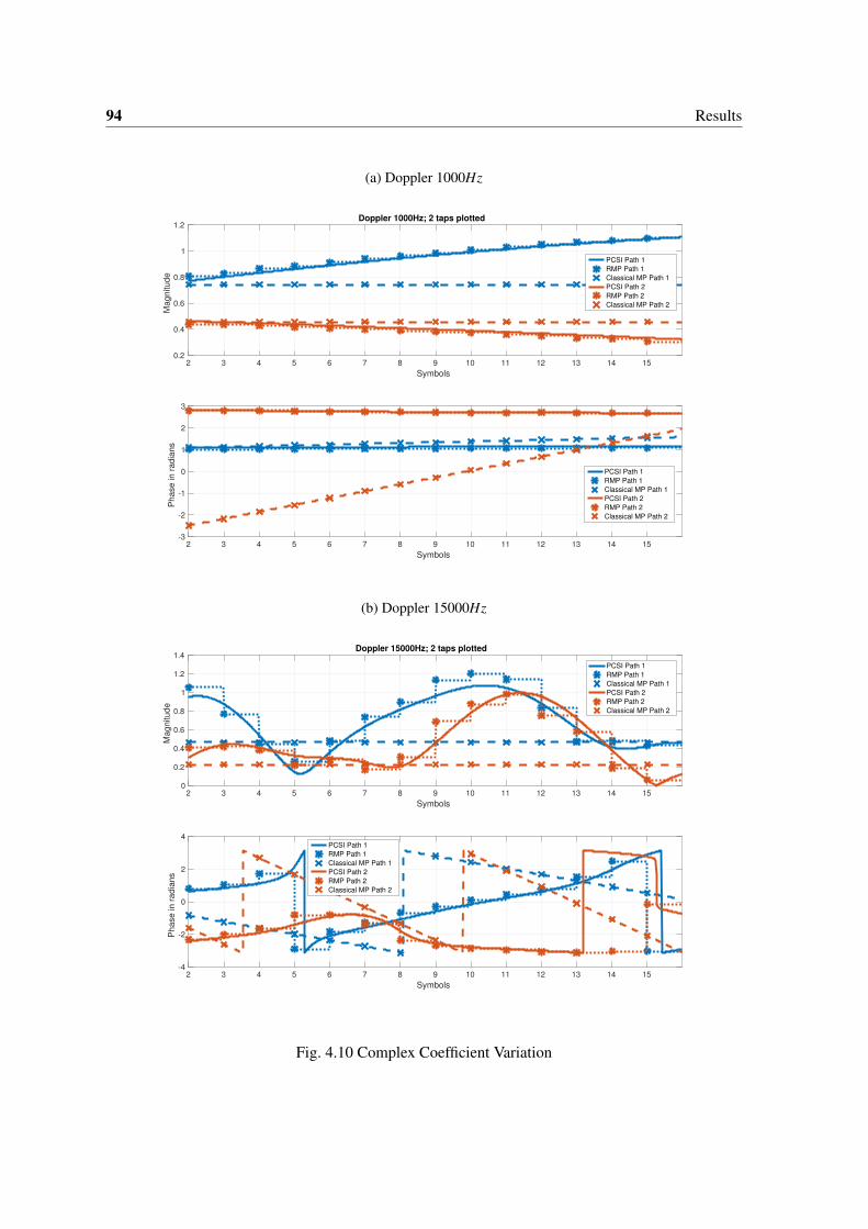
94 Results
(a) Doppler 1000Hz
2 3 4 5 6 7 8 9 10 11 12 13 14 15
Symbols
0.2
0.4
0.6
0.8
1
1.2
Magnitude
Doppler 1000Hz; 2 taps plotted
PCSI Path 1
RMP Path 1
Classical MP Path 1
PCSI Path 2
RMP Path 2
Classical MP Path 2
2 3 4 5 6 7 8 9 10 11 12 13 14 15
Symbols
-3
-2
-1
0
1
2
3
Phase in r
adia
ns
PCSI Path 1
RMP Path 1
Classical MP Path 1
PCSI Path 2
RMP Path 2
Classical MP Path 2
(b) Doppler 15000Hz
2 3 4 5 6 7 8 9 10 11 12 13 14 15
Symbols
0
0.2
0.4
0.6
0.8
1
1.2
1.4
Magnitude
Doppler 15000Hz; 2 taps plotted
PCSI Path 1
RMP Path 1
Classical MP Path 1
PCSI Path 2
RMP Path 2
Classical MP Path 2
2 3 4 5 6 7 8 9 10 11 12 13 14 15
Symbols
-4
-2
0
2
4
Phase in r
adia
ns
PCSI Path 1
RMP Path 1
Classical MP Path 1
PCSI Path 2
RMP Path 2
Classical MP Path 2
Fig. 4.10 Complex Coefficient Variation

4.4 RMP Performance 95
phase of the complex coefficient of both the dominant paths are not too pronounced. The magnitudeof xs using PCSI for the second symbol is fairly close to the magnitudes found by the classical MP forthese two paths. But, the classical MP retains these values for the entire frame and doesn’t updatethem, therefore the difference between the magnitudes gradually increases along the PHY frame.Contrarily, in the phase plot of Figure 4.10a, the classical MP finds the wrong phase for one of thepaths. The extension of the phase for the classical MP to all the following symbols is performed byusing the improvements described in subsection 3.5.3.
The RMP, however, exhibits accurate estimation of these coefficients for every OFDM symbol.The variation in both magnitude and phase is accurately estimated by the RMP algorithm as shown inFigure 4.10a. The step response of the RMP is due to the fact that it finds these coefficients once everyOFDM symbol and doesn’t update them within the symbol. In contrast, the channel is continuouslychanging which is clearly represented by the PCSI, but the RMP updates only at the intervals definedby the consecutive OFDM symbols. Each OFDM data symbol contains four pilots as defined bythe standard in subsection 2.2.3, but there are standards with much larger FFT size containing morenumber of pilots within an OFDM symbol. In such standards, the RMP can be modified to track thevariation of coefficients within the symbol. The core idea remains the same: search for the delaysusing a much larger set of defined sub-carriers, and then track the changes of the coefficients using asmaller set of defined sub-carriers (pilots).
For a high Doppler shift of 15000Hz, the step variation of the RMP is more evident, as shownin Figure 4.10b. The classical MP is inadequate in finding both the magnitude and phase variationsof the complex coefficients. However, the performance of the RMP in tracking the changes in bothmagnitude and phase under such high Doppler shifts is laudable. Thus, the outcome resembles thePCSI available for every OFDM symbol which includes the contributions from the multipath delaysand the corresponding Doppler shifts.
4.4 RMP Performance
A defined template of bytes is converted to the IEEE 802.11p PHY frame in the simulation platform.Multiple frames that are identical to each other are transmitted through a six path channel possessingtwo dominant paths. These two paths are characterized by an average power that is within 3dB of eachother. Noise is added in the channel by adopting the AWGN function of MATLAB in the ‘measured’mode. At the receiver, the received data is demodulated and the errors are calculated by comparingit with the template that was transmitted. Different Doppler shifts are simulated, and the errors arerecorded while increasing the SNR in steps of 3dB. The corresponding plots are shown in Figure 4.11.
For a purely multipath environment, as expected, the BER performance of all the three schemesare almost identical as shown in Figure 4.11a. This is in line with the observations obtained fromsection 4.2 and section 4.3. However, the better BER performance of the classical MP is surprising.This gain at lower SNRs could be due to the dual equalization, once in the frequency domain for themultipath delays, and another in the time domain for the Doppler as explained in subsection 3.5.3.

96 Results
(a) No Doppler
0 5 10 15 20 25 30
SNR (dB)
10 -4
10 -3
10 -2
10 -1
10 0
BE
R
Classical MP
RMP
LS
(b) Doppler 500Hz
0 5 10 15 20 25 30
SNR (dB)
10 -4
10 -3
10 -2
10 -1
10 0
BE
R
Classical MP
RMP
LS
(c) Doppler 1000Hz
0 5 10 15 20 25 30
SNR (dB)
10 -4
10 -3
10 -2
10 -1
10 0
BE
R
Classical MP
RMP
LS
(d) Doppler 5000Hz
0 5 10 15 20 25 30
SNR (dB)
10 -4
10 -3
10 -2
10 -1
10 0
BE
R
Classical MP
RMP
LS
(e) Doppler 10000Hz
0 5 10 15 20 25 30
SNR (dB)
10 -4
10 -3
10 -2
10 -1
10 0
BE
R
Classical MP
RMP
LS
(f) Doppler 15000Hz
0 5 10 15 20 25 30
SNR (dB)
10 -4
10 -3
10 -2
10 -1
10 0
BE
R
Classical MP
RMP
LS
Fig. 4.11 BER performance of RMP
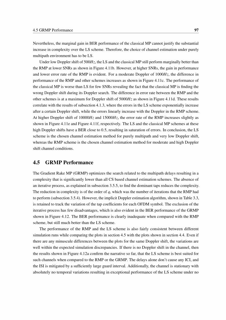
4.5 GRMP Performance 97
Nevertheless, the marginal gain in BER performance of the classical MP cannot justify the substantialincrease in complexity over the LS scheme. Therefore, the choice of channel estimation under purelymultipath environment has to be LS.
Under low Doppler shift of 500Hz, the LS and the classical MP still perform marginally better thanthe RMP at lower SNRs as shown in Figure 4.11b. However, at higher SNRs, the gain in performanceand lower error rate of the RMP is evident. For a moderate Doppler of 1000Hz, the difference inperformance of the RMP and other schemes increases as shown in Figure 4.11c. The performance ofthe classical MP is worse than LS for few SNRs revealing the fact that the classical MP is finding thewrong Doppler shift during its Doppler search. The difference in error rate between the RMP and theother schemes is at a maximum for Doppler shift of 5000Hz as shown in Figure 4.11d. These resultscorrelate with the results of subsection 4.1.3, where the errors in the LS scheme exponentially increaseafter a certain Doppler shift, while the errors linearly increase with the Doppler in the RMP scheme.At higher Doppler shift of 10000Hz and 15000Hz, the error rate of the RMP increases slightly asshown in Figure 4.11e and Figure 4.11f, respectively. The LS and the classical MP schemes at thesehigh Doppler shifts have a BER close to 0.5, resulting in saturation of errors. In conclusion, the LSscheme is the chosen channel estimation method for purely multipath and very low Doppler shift,whereas the RMP scheme is the chosen channel estimation method for moderate and high Dopplershift channel conditions.
4.5 GRMP Performance
The Gradient Rake MP (GRMP) optimizes the search related to the multipath delays resulting in acomplexity that is significantly lower than all CS based channel estimation schemes. The absence ofan iterative process, as explained in subsection 3.5.5, to find the dominant taps reduces the complexity.The reduction in complexity is of the order of q, which was the number of iterations that the RMP hadto perform (subsection 3.5.4). However, the implicit Doppler estimation algorithm, shown in Table 3.3,is retained to track the variation of the tap coefficients for each OFDM symbol. The exclusion of theiterative process has few disadvantages, which is also evident in the BER performance of the GRMPshown in Figure 4.12. The BER performance is clearly inadequate when compared with the RMPscheme, but still much better than the LS scheme.
The performance of the RMP and the LS scheme is also fairly consistent between differentsimulation runs while comparing the plots in section 4.5 with the plots shown in section 4.4. Even ifthere are any minuscule differences between the plots for the same Doppler shift, the variations arewell within the expected simulation discrepancies. If there is no Doppler shift in the channel, thenthe results shown in Figure 4.12a confirm the narrative so far, that the LS scheme is best suited forsuch channels when compared to the RMP or the GRMP. The delays alone don’t cause any ICI, andthe ISI is mitigated by a sufficiently large guard interval. Additionally, the channel is stationary withabsolutely no temporal variations resulting in exceptional performance of the LS scheme under no

98 Results
(a) No Doppler
0 5 10 15 20 25 30
SNR (dB)
10 -4
10 -3
10 -2
10 -1
10 0
BE
R
RMP
LS
GRMP
(b) Doppler 500Hz
0 5 10 15 20 25 30
SNR (dB)
10 -4
10 -3
10 -2
10 -1
10 0
BE
R
RMP
LS
GRMP
(c) Doppler 1000Hz
0 5 10 15 20 25 30
SNR (dB)
10 -4
10 -3
10 -2
10 -1
10 0
BE
R
RMP
LS
GRMP
(d) Doppler 5000Hz
0 5 10 15 20 25 30
SNR (dB)
10 -4
10 -3
10 -2
10 -1
10 0
BE
R
RMP
LS
GRMP
(e) Doppler 10000Hz
0 5 10 15 20 25 30
SNR (dB)
10 -4
10 -3
10 -2
10 -1
10 0
BE
R
RMP
LS
GRMP
(f) Doppler 15000Hz
0 5 10 15 20 25 30
SNR (dB)
10 -4
10 -3
10 -2
10 -1
10 0
BE
R
RMP
LS
GRMP
Fig. 4.12 BER performance of GRMP

4.6 Correlation Based Cognitive Framework Performance 99
Doppler shift channel conditions. From a low Doppler shift of 500Hz, the GRMP commences toperform better than the LS scheme as shown in Figure 4.12b.
A Doppler shift of 1000Hz is plenty enough to display the limitations of the LS scheme undermobility conditions as shown in Figure 4.12c. However, the favorable performance of the RMP undersuch conditions is clearly highlighted. The performance of the GRMP is relatively weaker than theRMP, which is as expected due to the marginal difference in finding the right delays in GRMP afterthe most dominant path. The additional paths, after the most dominant path, found by the RMPand GRMP vary marginally due to the absence of the iterative minimization in the GRMP method.The cost of performance for the gain in complexity between the RMP and GRMP is apparent, butnevertheless performance of GRMP is far greater than LS. This favors the use of the GRMP over theRMP method in consumer hardware, which is expected to work under high mobility conditions.
The performance gain over the LS scheme is even more pronounced in Figure 4.12d, Figure 4.12eand Figure 4.12f, when high Doppler shifts of 5000Hz, 10000Hz and 15000Hz are simulated, re-spectively. It is encouraging to note that the performance loss between the RMP and the GRMP isfairly consistent over different Doppler shifts. The order of difference in BER under various mobilityconditions between the RMP and GRMP is fairly independent of the magnitude of Doppler shift inthe channel. The GRMP has a lower complexity compared to the RMP algorithm and still maintainsadequate performance under high mobility conditions. The reduction in computational and memoryrequirements is a significant step towards the practical implementation of effective channel estimationschemes like the GRMP algorithm and enabling high mobility in consumer wireless communicationsystems.
4.6 Correlation Based Cognitive Framework Performance
The incentive to develop a cognitive framework is quite clear at this stage. Different channel estimationmethods do not offer reliable performance at optimum complexity under all channel conditions. Forinstance, the LS scheme exhibits acceptable performance only in low mobility environments. Onthe other hand, the RMP algorithm exhibits a significant gain in performance under high mobilityenvironments but at the cost of higher complexity. Moreover, under low mobility conditions RMPperforms relatively close to the LS, and thus its use in such environments is unjustified. The GRMPfollows on the same footsteps as the RMP, and therefore can replace the RMP as a high mobilityscheme if needed, without any change in the cognitive framework. Similarly, the low mobility schemechosen in this thesis is LS, but the cognitive framework is designed in a way that any suitable lowmobility scheme can be adopted.
The range of Doppler that is of interest for the cognitive framework is in the low and moderateDoppler range. Therefore, the Doppler shifts to be considered has changed from the previousexperiments. There are more sample Doppler shifts in the low and moderate range rather than thehigher range. The effectiveness of the cognitive framework needs to be evaluated for (i) performancein terms of the BER and (ii) the overall gain in complexity. The BER performance of the correlation

100 Results
(a) No Doppler
0 5 10 15 20 25 30
SNR
10 -4
10 -3
10 -2
10 -1
10 0
BE
R
Cognitive
RMP
LS
Ideal
(b) Doppler 100Hz
0 5 10 15 20 25 30
SNR
10 -4
10 -3
10 -2
10 -1
10 0
BE
R
Cognitive
RMP
LS
Ideal
(c) Doppler 300Hz
0 5 10 15 20 25 30
SNR
10 -4
10 -3
10 -2
10 -1
10 0
BE
R
Cognitive
RMP
LS
Ideal
(d) Doppler 700Hz
0 5 10 15 20 25 30
SNR
10 -4
10 -3
10 -2
10 -1
10 0
BE
R
Cognitive
RMP
LS
Ideal
(e) Doppler 1500Hz
0 5 10 15 20 25 30
SNR
10 -4
10 -3
10 -2
10 -1
10 0
BE
R
Cognitive
RMP
LS
Ideal
(f) Doppler 3000Hz
0 5 10 15 20 25 30
SNR
10 -4
10 -3
10 -2
10 -1
10 0
BE
R
Cognitive
RMP
LS
Ideal
Fig. 4.13 BER performance of Correlation Based Cognitive Framework

4.6 Correlation Based Cognitive Framework Performance 101
based cognitive framework, explained in subsection 3.6.1, is shown in Figure 4.13. The ideal cognitiveframework in Figure 4.13 is obtained in the simulations by performing the LS and the RMP channelestimation on the entire frame, and then finding the minimum of both errors. This ideal cognitiveframework forms the ground truth and its availability is restricted to simulations, and cannot beobtained in the real systems. In Figure 4.13a, a multipath environment is simulated, where theperformance of the RMP algorithm is comparable to that of LS in scenarios of low mobility. However,a closer look reveals that the LS scheme performs marginally better than the RMP in such conditions.Most importantly, the cognitive framework is able to accurately favor the LS scheme. This is alsoevident from Table 4.1 and Table 4.2 that shows the allocation (in %) of the two schemes underdifferent scenarios of mobility and SNR.
Table 4.1 Scheme’s percentages for Correlation Cognitive Framework (lower SNR)
Doppler (Hz) SchemeSNR (dB)
0 3 6 9 12 15
0LS 100% 96% 44% 93% 100% 100%RMP 0% 4% 56% 7% 0% 0%
100LS 12% 1% 25% 35% 51% 69%RMP 88% 99% 75% 65% 49% 31%
300LS 51% 11% 6% 5% 31% 75%RMP 49% 89% 94% 95% 69% 12%
700LS 47% 0% 0% 3% 1% 8%RMP 53% 100% 100% 97% 99% 92%
1500LS 1% 0% 0% 0% 0% 0%RMP 99% 100% 100% 100% 100% 100%
3000LS 70% 0% 0% 0% 0% 0%RMP 30% 100% 100% 100% 100% 100%
Table 4.1 shows the number of times the LS scheme was chosen (as a percentage) for differentDoppler shifts under low SNRs. The percentages were calculated by running the simulation platformfor 1000 frames, and increment the corresponding counters based on the scheme that was selectedby the cognitive framework. Then each counter value was divided by the total number of frames togive the percentage of frames that belonged to a particular scheme. The performance of the cognitiveframework for higher SNRs is shown in Table 4.2. Combining the plots in Figure 4.13, and thecorresponding rows in Table 4.1 and Table 4.2 gives a comprehensive analysis into the working ofthe correlation based cognitive framework. For a multipath environment, clearly the LS scheme isfavored, but for lower SNRs the cognitive framework doesn’t choose LS 100% of the time. Themetrics described in subsection 3.6.1 strives to choose the right scheme, but falls short of perfection.
For a very low Doppler of 100Hz, the cognitive framework still has to favor the LS scheme forBER performance as shown in Figure 4.13b. The cognitive framework achieves this competently for
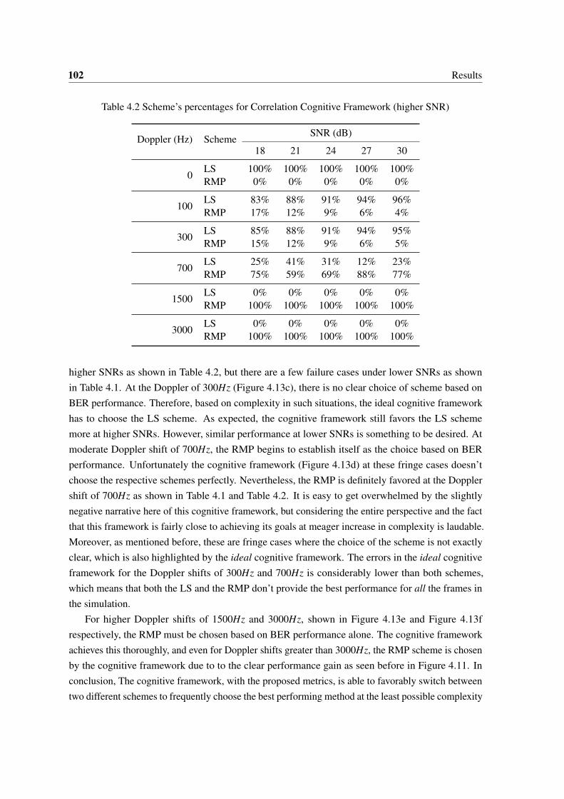
102 Results
Table 4.2 Scheme’s percentages for Correlation Cognitive Framework (higher SNR)
Doppler (Hz) SchemeSNR (dB)
18 21 24 27 30
0LS 100% 100% 100% 100% 100%RMP 0% 0% 0% 0% 0%
100LS 83% 88% 91% 94% 96%RMP 17% 12% 9% 6% 4%
300LS 85% 88% 91% 94% 95%RMP 15% 12% 9% 6% 5%
700LS 25% 41% 31% 12% 23%RMP 75% 59% 69% 88% 77%
1500LS 0% 0% 0% 0% 0%RMP 100% 100% 100% 100% 100%
3000LS 0% 0% 0% 0% 0%RMP 100% 100% 100% 100% 100%
higher SNRs as shown in Table 4.2, but there are a few failure cases under lower SNRs as shownin Table 4.1. At the Doppler of 300Hz (Figure 4.13c), there is no clear choice of scheme based onBER performance. Therefore, based on complexity in such situations, the ideal cognitive frameworkhas to choose the LS scheme. As expected, the cognitive framework still favors the LS schememore at higher SNRs. However, similar performance at lower SNRs is something to be desired. Atmoderate Doppler shift of 700Hz, the RMP begins to establish itself as the choice based on BERperformance. Unfortunately the cognitive framework (Figure 4.13d) at these fringe cases doesn’tchoose the respective schemes perfectly. Nevertheless, the RMP is definitely favored at the Dopplershift of 700Hz as shown in Table 4.1 and Table 4.2. It is easy to get overwhelmed by the slightlynegative narrative here of this cognitive framework, but considering the entire perspective and the factthat this framework is fairly close to achieving its goals at meager increase in complexity is laudable.Moreover, as mentioned before, these are fringe cases where the choice of the scheme is not exactlyclear, which is also highlighted by the ideal cognitive framework. The errors in the ideal cognitiveframework for the Doppler shifts of 300Hz and 700Hz is considerably lower than both schemes,which means that both the LS and the RMP don’t provide the best performance for all the frames inthe simulation.
For higher Doppler shifts of 1500Hz and 3000Hz, shown in Figure 4.13e and Figure 4.13frespectively, the RMP must be chosen based on BER performance alone. The cognitive frameworkachieves this thoroughly, and even for Doppler shifts greater than 3000Hz, the RMP scheme is chosenby the cognitive framework due to to the clear performance gain as seen before in Figure 4.11. Inconclusion, The cognitive framework, with the proposed metrics, is able to favorably switch betweentwo different schemes to frequently choose the best performing method at the least possible complexity

4.7 Complex Coefficient Based Cognitive Framework Performance 103
under appropriate channel conditions. This can also offer interesting advantages in battery drivenpractical systems by reducing the required computational power.
4.7 Complex Coefficient Based Cognitive Framework Performance
The complex coefficient (x) based cognitive framework is explained in subsection 3.6.2, and isexpected to be more robust to noise. The performance of this cognitive framework is anticipated tobe much better than the previous one even under low SNRs. The range of Doppler shifts are keptconsistent with respect to the simulations performed in section 4.6, so that comparison between thetwo different cognitive framework becomes easier. The process of evaluating the ideal cognitiveframework is also identical. The corresponding BER performance achieved by the complex coefficientbased cognitive framework is shown in Figure 4.14. The relevant percentage of the two differentschemes chosen by the cognitive framework for lower SNRs is given in Table 4.3. Similarly theselection efficiency for higher SNRs is given in Table 4.4.
The BER performance of the LS and the RMP under no Doppler channel condition is consistent,and therefore the cognitive framework has to select the LS scheme. The previous cognitive frameworkhad the issue of selecting the RMP at lower SNRs as shown in Table 4.1. But, the improved frameworkthat is dependent on x is almost perfect, as it selects the LS scheme 100% of the time barring thecondition when the SNR is 0dB. For a very low Doppler of 100Hz, the improved metric continues tooutperform the previous method, as it manages to select the LS scheme consistently when the SNR isgreater than 6dB (Table 4.3). In comparison, the previous method chose the RMP more often evenunder higher SNRs.
Table 4.3 Scheme’s percentages for x Cognitive Framework (lower SNR)
Doppler (Hz) SchemeSNR (dB)
0 3 6 9 12 15
0LS 79% 100% 100% 100% 100% 100%RMP 21% 0% 0% 0% 0% 0%
100LS 8% 50% 97% 100% 100% 100%RMP 92% 50% 3% 0% 0% 0%
300LS 3% 56% 91% 11% 60% 100%RMP 97% 44% 9% 89% 40% 0%
700LS 0% 1% 3% 0% 1% 3%RMP 100% 99% 97% 100% 99% 97%
1500LS 0% 0% 0% 0% 0% 0%RMP 100% 100% 100% 100% 100% 100%
3000LS 0% 0% 0% 0% 0% 0%RMP 100% 100% 100% 100% 100% 100%

104 Results
(a) No Doppler
0 5 10 15 20 25 30
SNR
10 -4
10 -3
10 -2
10 -1
10 0
BE
R
Cognitive
RMP
LS
Ideal
(b) Doppler 100Hz
0 5 10 15 20 25 30
SNR
10 -4
10 -3
10 -2
10 -1
10 0
BE
R
Cognitive
RMP
LS
Ideal
(c) Doppler 300Hz
0 5 10 15 20 25 30
SNR
10 -4
10 -3
10 -2
10 -1
10 0
BE
R
Cognitive
RMP
LS
Ideal
(d) Doppler 700Hz
0 5 10 15 20 25 30
SNR
10 -4
10 -3
10 -2
10 -1
10 0
BE
R
Cognitive
RMP
LS
Ideal
(e) Doppler 1500Hz
0 5 10 15 20 25 30
SNR
10 -4
10 -3
10 -2
10 -1
10 0
BE
R
Cognitive
RMP
LS
Ideal
(f) Doppler 3000Hz
0 5 10 15 20 25 30
SNR
10 -4
10 -3
10 -2
10 -1
10 0
BE
R
Cognitive
RMP
LS
Ideal
Fig. 4.14 BER performance of x Based Cognitive Framework

4.7 Complex Coefficient Based Cognitive Framework Performance 105
Table 4.4 Scheme’s percentages for x Cognitive Framework (higher SNR)
Doppler (Hz) SchemeSNR (dB)
18 21 24 27 30
0LS 100% 100% 100% 100% 100%RMP 0% 0% 0% 0% 0%
100LS 100% 100% 100% 100% 100%RMP 0% 0% 0% 0% 0%
300LS 100% 100% 100% 100% 100%RMP 0% 0% 0% 0% 0%
700LS 2% 1% 4% 0% 2%RMP 98% 99% 96% 100% 98%
1500LS 0% 0% 0% 0% 0%RMP 100% 100% 100% 100% 100%
3000LS 0% 0% 0% 0% 0%RMP 100% 100% 100% 100% 100%
The major points of contention are the fringe cases of 300Hz and 700Hz. As mentioned before,the BER performance shown in Figure 4.14 suggests that, for a Doppler of 300Hz the performance ofthe LS and RMP are almost identical. Therefore the cognitive framework has to instead select LSto achieve lowest complexity. The x based method clearly outperforms the previous method even inthe fringe case of 300Hz by selecting the LS scheme 100% of the time for higher SNRs (Table 4.4).Even under lower SNRs, the x method (Table 4.3) performs better than the correlation based cognitiveframework (Table 4.1). A substantial improvement is witnessed in the fringe case of 700Hz too,both in BER performance (Figure 4.14d) and in the selection of the RMP (Table 4.3, Table 4.4),when compared to the previous method that showed significant degradation in BER performance(Figure 4.13d). For higher Doppler shifts of 1500Hz (Figure 4.14e) and 3000Hz (Figure 4.14f), thebehavior resembles the previous method, and is indistinguishable from the ideal cognitive framework.Displaying the performance of both cognitive frameworks for Doppler shifts beyond 3000Hz areredundant as the selection is always RMP in those cases, and both have been confirmed to accomplishthe same in simulations.
In conclusion, the x based cognitive framework achieves much better performance at a loweroverhead complexity of O(N +q). In comparison, the correlation based cognitive framework has acomplexity of O(4N +q) and is sensitive to noise. The goal, that was set out at the beginning, wasto construct an ideal cognitive framework that can detect the different channel conditions, and notnecessarily estimate them, at a marginal increase in complexity. This needed to facilitate the switchbetween different channel estimation methods to consistently provide good performance at optimumcomplexity. This was, and still is, not a trivial problem, but this thesis has gotten extremely close tothe perfect solution.


The pursuit of truth and beauty is a sphereof activity in which we are permitted toremain children all our lives.
Albert Einstein
Part V
The Resolution
107

CHAPTER 5CONCLUSION
With the advent of all major car makers pursuing an effective self driving system, it is imperativethat a vehicular communication system, which is functional even in the harshest of environments,is in place for maximum safety. Channel estimation and channel equalization are one of the mostimportant system blocks in a communication system to deal with the high mobility environmentof the vehicular communication system. The various innovations proposed in this thesis provideadequate solutions to handle the dynamic environment. As of writing this thesis, the novel ideaspresented have been part of three research papers submitted in three different conferences. Theprocess of review and acceptance for first conference, European Conference on Networks andCommunications (EuCNC 2017, Oulu, Finland), has already been completed in [16]. Recently, theprocess of review and acceptance for second conference, Vehicular Technology Conference (VTC2017-Fall, Toronto, Canada), has also been completed [138]. The process for the other conference,International Conference of Consumer Electronics (ICCE-Berlin 2017, Berlin, Germany), is yet to becompleted and corresponding acceptance is awaited.
5.1 Contributions
This thesis provides a robust channel estimation scheme, the RMP, that works significantly betterin scenarios of high mobility. The proposed scheme not only improves the performance of existingmulticarrier systems but also provides greater flexibility in the design of telecommunication systemsfor the future. Although the proposed technique is implemented for the IEEE 802.11p standard, it issuitable for any OFDM based multicarrier system that has to cope with high mobility and/or workreliably at higher frequencies. The complexity of RMP is also lower than the previous CS basedmatching pursuit algorithms. Hence, it provides an efficient channel estimation scheme that worksentirely in the frequency domain while implicitly estimating the Doppler in the channel. Results haveshown that the channel transfer function obtained from the RMP is close to the Perfect Channel StateInformation for rapidly varying channels. The RMP is also simulated on an open-source platform toverify the performance over different programs.

110 Conclusion
Furthermore, the thesis investigated the complexity and storage demands associated with thedictionary, which are often assumed to be available in the MP algorithms. It is shown that thegeneration of the dictionary requires significant computational and memory resources. Then, a novelscheme to build the dictionary using the concept of wavelets is presented, which can be used by anyCS based channel estimation algorithms. The advantages in complexity and storage requirements forboth the time domain and frequency domain dictionaries are highlighted.
The thesis also proposes a novel delay search method, GRMP, that has a lower complexitycompared to the RMP algorithm and still maintains adequate performance under high mobilityconditions. Exploiting the non-iterative process of the GRMP, a deterministic bound on the executiontime can also be calculated for the entire algorithm at the receiver. Additionally, as a contribution tothe community, the IEEE 802.11p simulation tool is now open source and is available for downloadfor further experimental research.
The narrative that the channel estimation methods don’t provide suitable performance at optimumcomplexity for all channel conditions has been confirmed through rigorous simulations. Therefore, thecorrelation based cognitive framework, along-with the metrics, have been defined to switch betweena low and high mobility channel estimation methods depending on the channel conditions. Withthis cognitive framework, ample gain in complexity is achieved by switching to a less complexmethod under low mobility conditions. To improve the performance of the cognitive frameworkfurther, the complex coefficient based cognitive framework has been proposed. This provides uswith a channel estimation scheme that is robust, precise and reliable in all channel conditions whileadapting the complexity to be optimal for the channel being estimated. Combining all the incrementalimprovements, this thesis takes a giant leap towards enabling high mobility in the communicationsystem and its practical implementation on consumer hardware.
5.2 Future Work
The main goal of this thesis was to provide the cognitive framework to enable adequate channelestimation and equalization in all mobility conditions. Although this goal has been achieved andproved through simulations, there is still research to be performed on hardware applicability and thecorresponding issues that might arise. The USRP could provide an intermediate step in this directionon both MATLAB and GNU Radio platforms. Implementing the algorithms on both platforms andtesting them with the USRP will provide higher confidence on the performance before investingheavily on hardware. The immediate step would therefore be to continue the work on GNU Radio toinclude all the improvements and implement the cognitive framework.
The information provided by the RMP could be extended to other equalization techniques (sub-section 2.9.3) to either reduce complexity or improve the equalization performance. The informationof delays and its corresponding coefficients could also be transferred back to the time domain thatcan be used to reconstruct a filter for each OFDM symbol, which might provide better equalizationperformance. There are other MP algorithms too that claim to offer better performance as mentioned

5.2 Future Work 111
in subsection 2.8.4. These MP algorithms could be implemented and evaluated easily in MATLABthanks to the simulation platform developed as part of this thesis. The simulation platform could alsobe extended to include higher layers of the IEEE 1609 to estimate the overall performance of theentire stack of protocols.
The cognitive framework could be extended to include more Intra-Frame cognition. The highmobility method like RMP could be invoked for intermittent OFDM symbols under moderate mobilityinstead of invoking it for every OFDM symbol and thus achieve modest gains in complexity. All ofthe methods and algorithms proposed in this thesis can be implemented and evaluated for differentstandards, like DVB-T2, that employ OFDM in the PHY layer. Likewise, further research in differentaspects of this thesis can be continued in divergent directions, which leads to the following concludingquote.
The outcome of any serious research canonly be to make two questions grow whereonly one grew before.
Thorstein Veblen


REFERENCES
[1] Hope Reese. Tesla driver dies in first fatality with Autopilot: What it means for the future ofdriverless cars. 2016. URL: http://www.techrepublic.com/article/tesla-driver-dies-in-first-fatality-with-autopilot-what-it-means-for-the-future-of-driverless-cars/.
[2] Huei Peng. Saving lives by letting cars talk to each other. 2016. URL: http://theconversation.com/saving-lives-by-letting-cars-talk-to-each-other-59221.
[3] Claudio Rebuzzi. CAR-2-CAR Communication is the autonomous future of driving. 2013.URL: http://motorburn.com/2013/03/car-2-car-communication-is-the-autonomous-future-of-driving/.
[4] U.S. Department of Transportation (US DOT). Vehicle-to-Pedestrian (V2P) Communicationsfor Safety. [Online; accessed 4-May-2017]. 2017. URL: https://www.its.dot.gov/research_archives/safety/v2p_comm_safety.htm.
[5] U.S. Department of Transportation (US DOT). Vehicle-to-Infrastructure (V2I) Communi-cations for Safety. [Online; accessed 4-May-2017]. 2017. URL: https://www.its.dot.gov/research_archives/safety/v2i_comm_safety.htm.
[6] U.S. Department of Transportation (US DOT). Vehicle-to-Vehicle (V2V) Communicationsfor Safety. [Online; accessed 4-May-2017]. 2017. URL: https://www.its.dot.gov/research_archives/safety/v2v_comm_safety.htm.
[7] Robert F.H. Fischer and Clemens Stierstorfer. “Single- vs. Multicarrier Transmission inMIMO and Multiuser Scenarios”. In: OFDM - Concepts for Future Communication Systems.Ed. by H. Rohling. 1st ed. Signals and Communication Technology. Berlin, Heidelberg:Springer Verlag, May 2011, pp. 5–20. DOI: 10.1007/978-3-642-17496-4_3.
[8] CAR 2 CAR Communication Consortium. Car-2-Car. 2015. URL: https://www.car-2-car.org.
[9] Diego A. Samo, Mariem Slimani, Giuseppe Baruffa, and Luca Rugini. “A performance studyof DVB-T2 and DVB-T2-Lite for mobile reception”. In: Digital Signal Processing 37 (2015),pp. 35 –42. ISSN: 1051-2004.
[10] IEEE. Part 11: Wireless LAN Medium Access Control(MAC) and Physical Layer (PHY)Specifications, IEEE802.11-2012. 2012. URL: https://standards.ieee.org/findstds/standard/802.11-2012.html.

114 References
[11] IEEE. Part 11: Wireless LAN Medium Access Control (MAC) and Physical Layer (PHY)Specifications Amendment 3: Enhancements for Very High Throughput in the 60 GHz Band.2012. URL: https://standards.ieee.org/findstds/standard/802.11ad-2012.html.
[12] Ian F. Akyildiz, Shuai Nie, Shih-Chun Lin, and Manoj Chandrasekaran. “5G Roadmap”. In:The International Journal of Computer and Telecommunications Networking 106.C (Sept.2016), pp. 17–48.
[13] Huawei. 5G: New Air Interface and Radio Access Virtualization. http://www.huawei.com/minisite/has2015/img/5g_radio_whitepaper.pdf. 2015.
[14] Digital Video Broadcasting Project (DVB). DVB-T2 Standard. 2010. URL: https://www.dvb.org/standards/dvb-t2.
[15] Nasimi Eldarov, Guoping Tan, and Thorsten Herfet. “High mobility in OFDM systems basedon FFT”. In: 2015 IEEE International Conference on Consumer Electronics (ICCE). IEEE.2015, pp. 414–415.
[16] Kelvin Chelli, Praharsha Sirsi, and Thorsten Herfet. “Sparse Doubly-Selective Channels:Estimating Path Parameters Unambiguously”. In: 2017 European Conference on Networksand Communications (EuCNC): Physical Layer and Fundamentals (PHY) (EuCNC2017 -PHY). Oulu, Finland, June 2017.
[17] D. Needell and J.A. Tropp. “CoSaMP: Iterative signal recovery from incomplete and inaccu-rate samples”. In: Applied and Computational Harmonic Analysis 26.3 (2009), pp. 301 –321.ISSN: 1063-5203.
[18] A. Das, W. S. Hodgkiss, and P. Gerstoft. “Coherent Multipath Direction-of-Arrival ResolutionUsing Compressed Sensing”. In: IEEE Journal of Oceanic Engineering 42.2 (Apr. 2017),pp. 494–505. ISSN: 0364-9059. DOI: 10.1109/JOE.2016.2576198.
[19] Gitta Kutyniok. “Theory and applications of compressed sensing”. In: GAMM-Mitteilungen36.1 (2013), pp. 79–101. ISSN: 1522-2608. DOI: 10.1002/gamm.201310005. URL: http://dx.doi.org/10.1002/gamm.201310005.
[20] Weichang Li and James C Preisig. “Estimation of rapidly time-varying sparse channels”. In:IEEE Journal of Oceanic Engineering 32.4 (2007), pp. 927–939.
[21] G. Tan and T. Herfet. “A Framework of Analyzing OMP-Based Channel Estimations in MobileOFDM Systems”. In: IEEE Wireless Communications Letters 5.4 (Aug. 2016), pp. 408–411.ISSN: 2162-2337. DOI: 10.1109/LWC.2016.2571688.
[22] Kelvin Chelli and Thorsten Herfet. “Doppler Shift Compensation in Vehicular CommunicationSystems”. In: International Conference on Computer and Communications (ICCC). Chengdu,Oct. 2016.
References 115
[23] European Commission. 2008/671/EC: Commission Decision of 5 August 2008 on the har-monised use of radio spectrum in the 5875 - 5905 MHz frequency band for safety-relatedapplications of Intelligent Transport Systems (ITS). 2008. URL: http://eur-lex.europa.eu/legal-content/EN/TXT/PDF/?uri=CELEX:32008D0671&from=EN.
[24] Associated Press. Cars are ready to talk to one another — unless we use their airwaves forWi-Fi. 2016. URL: http://www.latimes.com/business/autos/la-fi-hy-talking-cars-20160825-snap-story.html.
[25] IEEE. Official IEEE 802.11 Working Group Project Timelines. 2016. URL: http://grouper.ieee.org/groups/802/11/Reports/802.11_Timelines.htm.
[26] IEEE. Official IEEE 802.11 Working Group Project Timelines. 2010. URL: http://grouper.ieee.org/groups/802/11/Reports/tgp_update.htm.
[27] Claude Elwood Shannon. “A mathematical theory of communication”. In: ACM SIGMOBILEMobile Computing and Communications Review 5.1 (2001), pp. 3–55.
[28] Robert W Chang. “Synthesis of Band-Limited Orthogonal Signals for Multichannel DataTransmission”. In: Bell System Technical Journal 45.10 (1966), pp. 1775–1796.
[29] Irving Kalet. “The multitone channel”. In: IEEE Transactions on Communications 37.2 (1989),pp. 119–124.
[30] Taewon Hwang, Chenyang Yang, Gang Wu, Shaoqian Li, and Geoffrey Ye Li. “OFDM and itswireless applications: a survey”. In: IEEE transactions on Vehicular Technology 58.4 (2009),pp. 1673–1694.
[31] Jean Armstrong. “OFDM for optical communications”. In: Journal of lightwave technology27.3 (2009), pp. 189–204.
[32] Thorsten Herfet. Telecommunications 2 Audio - Visual Communications and Networks.Telecommunications Lab, Universität des Saarlandes, 2016.
[33] Ferdinand Classen and Heinrich Meyr. “Frequency synchronization algorithms for OFDMsystems suitable for communication over frequency selective fading channels”. In: VehicularTechnology Conference, 1994 IEEE 44th. IEEE. 1994, pp. 1655–1659.
[34] Timothy M Schmidl and Donald C Cox. “Robust frequency and timing synchronization forOFDM”. In: IEEE transactions on communications 45.12 (1997), pp. 1613–1621.
[35] Thorsten Herfet. Telecommunications 1 Digital Transmission and Signal Processing. Telecom-munications Lab, Universität des Saarlandes, 2016.
[36] Leonard Cimini. “Analysis and simulation of a digital mobile channel using orthogonalfrequency division multiplexing”. In: IEEE transactions on communications 33.7 (1985),pp. 665–675.

116 References
[37] Zijun Zhao, Xiang Cheng, Miaowen Wen, Bingli Jiao, and Cheng-Xiang Wang. “Channelestimation schemes for IEEE 802.11 p standard”. In: IEEE Intelligent Transportation SystemsMagazine 5.4 (2013), pp. 38–49.
[38] Jorg Nuckelt, Moritz Schack, and Thomas Kurner. “Performance evaluation of wiener filter de-signs for channel estimation in vehicular environments”. In: Vehicular Technology Conference(VTC Fall), 2011 IEEE. IEEE. 2011, pp. 1–5.
[39] Stéphane G Mallat and Zhifeng Zhang. “Matching pursuits with time-frequency dictionaries”.In: IEEE Transactions on signal processing 41.12 (1993), pp. 3397–3415.
[40] Emmanuel J Candès and Michael B Wakin. “An introduction to compressive sampling”. In:IEEE signal processing magazine 25.2 (2008), pp. 21–30.
[41] T. Hrycak, S. Das, G. Matz, and H. G. Feichtinger. “Low Complexity Equalization forDoubly Selective Channels Modeled by a Basis Expansion”. In: IEEE Transactions on SignalProcessing 58.11 (Nov. 2010), pp. 5706–5719. ISSN: 1053-587X. DOI: 10.1109/TSP.2010.2063426.
[42] Georg Taubock, Franz Hlawatsch, Daniel Eiwen, and Holger Rauhut. “Compressive estimationof doubly selective channels in multicarrier systems: Leakage effects and sparsity-enhancingprocessing”. In: IEEE Journal of Selected Topics in Signal Processing 4.2 (2010), pp. 255–271.
[43] Mark A Davenport, Marco F Duarte, Yonina C Eldar, and Gitta Kutyniok. “Introduction tocompressed sensing”. In: Preprint 93.1 (2011), p. 2.
[44] R. Hicheri, M. Paetzold, and N. Youssef. “On the statistical properties of the capacity of sparsemultipath fading channels”. In: 2014 International Conference on Advanced Technologies forCommunications (ATC 2014). Oct. 2014, pp. 338–343. DOI: 10.1109/ATC.2014.7043408.
[45] Michal Simko, Paulo SR Diniz, Qi Wang, and Markus Rupp. “Adaptive pilot-symbol patternsfor MIMO OFDM systems”. In: IEEE Transactions on Wireless Communications 12.9 (2013),pp. 4705–4715.
[46] Chenhao Qi, Guosen Yue, Lenan Wu, and Arumugam Nallanathan. “Pilot design for sparsechannel estimation in OFDM-based cognitive radio systems”. In: IEEE Transactions onVehicular Technology 63.2 (2014), pp. 982–987.
[47] Joel A Tropp and Anna C Gilbert. “Signal recovery from random measurements via orthogonalmatching pursuit”. In: IEEE Transactions on information theory 53.12 (2007), pp. 4655–4666.
[48] Scott Shaobing Chen, David L Donoho, and Michael A Saunders. “Atomic decomposition bybasis pursuit”. In: SIAM review 43.1 (2001), pp. 129–159.
[49] David L Donoho. “Compressed sensing”. In: IEEE Transactions on information theory 52.4(2006), pp. 1289–1306.

References 117
[50] Joel A Tropp. “Greed is good: Algorithmic results for sparse approximation”. In: IEEETransactions on Information theory 50.10 (2004), pp. 2231–2242.
[51] Nasimi Eldarov, Guoping Tan, and Thorsten Herfet. “Delay-Doppler search for matchingpursuit algorithms in time-variant channels”. In: 2015 IEEE International Symposium onBroadband Multimedia Systems and Broadcasting. IEEE. 2015, pp. 1–5.
[52] W. Dai and O. Milenkovic. “Subspace Pursuit for Compressive Sensing Signal Reconstruc-tion”. In: IEEE Transactions on Information Theory 55.5 (May 2009), pp. 2230–2249. ISSN:0018-9448. DOI: 10.1109/TIT.2009.2016006.
[53] Lang Tong, Guanghan Xu, and Thomas Kailath. “Blind identification and equalization basedon second-order statistics: A time domain approach”. In: IEEE Transactions on informationTheory 40.2 (1994), pp. 340–349.
[54] Christian Rohde, Wolfgang Gerstacker, Bernhard Schmidt, and Wolfgang Koch. “Comparisonof One-Dimensional Adaptive Channel Estimation Techniques for OFDM Systems”. In: Proc.InOWo 2008, International OFDM-Workshop, pp. 110–114.
[55] Kelvin Chelli. “Doppler Shift Compensation in Vehicular Communication Systems”. MasterThesis. Department of Computer Science, Saarland University, Mar. 2015.
[56] Nikolaos I Miridakis and Dimitrios D Vergados. “A survey on the successive interferencecancellation performance for single-antenna and multiple-antenna OFDM systems”. In: IEEECommunications Surveys & Tutorials 15.1 (2013), pp. 312–335.
[57] Youssef El Hajj Shehadeh, Sebastian Bamgartner, Danai Chasaki, and Gangolf Hirtz. “Lowcomplexity Intercarrier Interference reduction for high mobility wireless systems”. In: 2015IEEE International Conference on Consumer Electronics (ICCE). IEEE. 2015, pp. 641–644.
[58] Christopher C Paige and Michael A Saunders. “LSQR: An algorithm for sparse linear equa-tions and sparse least squares”. In: ACM transactions on mathematical software 8.1 (1982),pp. 43–71.
[59] Tomasz Hrycak and Gerald Matz. “Low-complexity time-domain ICI equalization for OFDMcommunications over rapidly varying channels”. In: 2006 Fortieth Asilomar Conference onSignals, Systems and Computers. IEEE. 2006, pp. 1767–1771.
[60] David Chin-Lung Fong and Michael Saunders. “LSMR: An iterative algorithm for sparseleast-squares problems”. In: SIAM Journal on Scientific Computing 33.5 (2011), pp. 2950–2971.
[61] Georg Taubock, Mario Hampejs, Gerald Matz, Franz Hlawatsch, and Karlheinz Grochenig.“LSQR-based ICI equalization for multicarrier communications in strongly dispersive andhighly mobile environments”. In: 2007 IEEE 8th Workshop on Signal Processing Advances inWireless Communications. IEEE. 2007, pp. 1–5.

118 References
[62] F Nyongesa, K Djouani, T Olwal, and Y Hamam. “Doppler shift compensation schemes inVANETs”. In: Mobile Information Systems 2015 (2015).
[63] Bor-Sen Chen and Jung-Feng Liao. “Adaptive MC-CDMA multiple channel estimation andtracking over time-varying multipath fading channels”. In: IEEE Transactions on wirelesscommunications 6.6 (2007).
[64] Rocco Claudio Cannizzaro, Paolo Banelli, and Geert Leus. “Adaptive channel estimation forOFDM systems with Doppler spread”. In: Signal Processing Advances in Wireless Communi-cations, 2006. SPAWC’06. IEEE 7th Workshop on. IEEE. 2006, pp. 1–5.
[65] Takeshi Onizawa, Masato Mizoguchi, Tetsu Sakata, and Masahiro Morikura. “A simple adap-tive channel estimation scheme for OFDM systems”. In: Vehicular Technology Conference,1999. VTC 1999-Fall. IEEE VTS 50th. Vol. 1. IEEE. 1999, pp. 279–283.
[66] Xenofon G Doukopoulos and George V Moustakides. “Blind adaptive channel estimation inOFDM systems”. In: IEEE Transactions on Wireless Communications 5.7 (2006), pp. 1716–1725.
[67] Katrin Bilstrup, Elisabeth Uhlemann, Erik G Strom, and Urban Bilstrup. “Evaluation of theIEEE 802.11 p MAC method for vehicle-to-vehicle communication”. In: Vehicular TechnologyConference, 2008. VTC 2008-Fall. IEEE 68th. IEEE. 2008, pp. 1–5.
[68] Joseph A Fernandez, Kevin Borries, Lin Cheng, BVK Vijaya Kumar, Daniel D Stancil, andFan Bai. “Performance of the 802.11 p physical layer in vehicle-to-vehicle environments”. In:IEEE Transactions on Vehicular Technology 61.1 (2012), pp. 3–14.
[69] Samaneh Shooshtary. Development of a MATLAB simulation environment for vehicle-to-vehicle and infrastructure communication based on IEEE 802.11 p. 2008.
[70] Claudia Campolo, Alexey Vinel, Antonella Molinaro, and Yevgeni Koucheryavy. “Modelingbroadcasting in IEEE 802.11 p/WAVE vehicular networks”. In: IEEE Communications Letters15.2 (2011), pp. 199–201.
[71] Martin Clark. IEEE 802.11a WLAN model. 2016. URL: http://bit.ly/2pnehrn.
[72] MathWorks. 802.11p and 802.11a Packet Error Rate Simulations. 2017. URL: https://in.mathworks.com/help/wlan/examples/802-11p-and-802-11a-packet-error-rate-simulations.html.
[73] Oliver Haffenden. DVB-T2: The Common Simulation Platform. http://downloads.bbc.co.uk/rd/pubs/whp/whp-pdf-files/WHP196.pdf. 2011.
[74] Kelvin Chelli, Praharsha Sirsi, Ramzi Theodory, and Thorsten Herfet. IEEE 802.11p Simu-lation Platform. (2017) [Online]. Available: https://git.nt.uni-saarland.de/HiMo/SimTool_IEEE802.11p. Accessed on: Mar.28, 2017.
[75] Michel C Jeruchim, Philip Balaban, and K Sam Shanmugan. Simulation of communicationsystems: modeling, methodology and techniques. Springer Science & Business Media, 2006.

References 119
[76] Peter Almers, Ernst Bonek, A Burr, Nicolai Czink, Mérouane Debbah, Vittorio Degli-Esposti,Helmut Hofstetter, Pekka Kyösti, D Laurenson, Gerald Matz, et al. “Survey of channel andradio propagation models for wireless MIMO systems”. In: EURASIP Journal on WirelessCommunications and Networking 2007.1 (2007), pp. 56–56.
[77] Muhammad Imran, Abas Md Said, and Halabi Hasbullah. “A survey of simulators, emula-tors and testbeds for wireless sensor networks”. In: Information Technology (ITSim), 2010International Symposium in. Vol. 2. IEEE. 2010, pp. 897–902.
[78] William C Jakes and Donald C Cox. Microwave mobile communications. Wiley-IEEE Press,1994.
[79] MathWorks. Fading Channels. 2017. URL: https://in.mathworks.com/help/comm/ug/fading-channels.html.
[80] M Failli and Generaldirektion Telekommunikation Europäische Gemeinschaften. Digital landmobile radio communications: COST 207; final report (14 March 1984-13 Sept. 1988). Officefor Office Publ. of the European Communities, 1989.
[81] European Telecommunications Standards Institute. Digital cellular telecommunications sys-tem (Phase 2+); Radio transmission and reception (3GPP TS 45.005 version 7.14.0 Release7). 2008. URL: http://www.etsi.org/deliver/etsi_ts/145000_145099/145005/07.14.00_60/ts_145005v071400p.pdf.
[82] M Series. “Guidelines for evaluation of radio interface technologies for IMT-Advanced”. In:Report ITU 2135-1 (2009).
[83] ETSI Normalization Committee et al. “Channel models for HIPERLAN/2 in different indoorscenarios”. In: Norme ETSI, document 3ERI085B, European Telecommunications StandardsInstitute, Sophia-Antipolis, Valbonne, France 1 (1998).
[84] Tore Ulversoy. “Software defined radio: Challenges and opportunities”. In: IEEE Communica-tions Surveys & Tutorials 12.4 (2010), pp. 531–550.
[85] Bastian Bloessl, Michele Segata, Christoph Sommer, and Falko Dressler. “An IEEE 802.11a/g/p OFDM Receiver for GNU Radio”. In: Proceedings of the second workshop on Softwareradio implementation forum. ACM. 2013, pp. 9–16.
[86] Bastian Bloessl, Michele Segata, Christoph Sommer, and Falko Dressler. “Towards an opensource IEEE 802.11 p stack: a full sdr-based transceiver in gnu radio”. In: 2013 IEEE VehicularNetworking Conference. IEEE. 2013, pp. 143–149.
[87] IEEE. IEEE Standard for Air Interface for Broadband Wireless Access Systems. 2012. URL:https://standards.ieee.org/getieee802/download/802.16-2012.pdf.
[88] IEEE. Part 15.3: Wireless Medium Access Control (MAC) and Physical Layer (PHY) Spec-ifications for High Rate Wireless Personal Area Networks (WPANs). 2009. URL: https: / /standards.ieee.org/getieee802/download/802.15.3c-2009.pdf.

120 References
[89] IEEE. TS 36.201, 3rd Generation Partnership Project (3GPP), LTE; Evolved UniversalTerrestrial Radio Access (E-UTRA); Long Term Evolution (LTE) physical layer; Generaldescription (3GPP TS 36.201 version 8.3.0 Release 8). 2009. URL: http://www.etsi.org/deliver/etsi_ts/136200_136299/136201/08.03.00_60/ts_136201v080300p.pdf.
[90] Philip Schniter, Sung-Jun Hwang, Sibasish Das, and Arun P Kannu. “Equalization of time-varying channels”. In: Wireless Communications over Rapidly Time-Varying Channels 6(2011), pp. 237–283.
[91] Federal Communications Commission. FCC allocates spectrum in 5.9 GHz range for Intelli-gent Transportation Systems uses. 1999. URL: https://transition.fcc.gov/Bureaus/Engineering_Technology/News_Releases/1999/nret9006.html.
[92] Yunxin Jeff Li. “An overview of the DSRC/WAVE technology”. In: International Conferenceon Heterogeneous Networking for Quality, Reliability, Security and Robustness. Springer.2010, pp. 544–558.
[93] AM Abdelgader and Wu Lenan. “The physical layer of the IEEE 802.11 p WAVE communi-cation standard: the specifications and challenges”. In: Proceedings of the World Congress onEngineering and Computer Science. Vol. 2. 2014.
[94] Prasan Kumar Sahoo, Ming-Jer Chiang, and Shih-Lin Wu. “SVANET: A Smart VehicularAd Hoc Network for Efficient Data Transmission with Wireless Sensors”. In: Sensors 14.12(2014), pp. 22230–22260.
[95] Gaurav Pathak. IEEE 802.11P: Wireless Access in Vehicular Environment. 2015. URL: https://gauravpathak07.wordpress.com/.
[96] Pieter van Wijngaarden. “Frame Capture in IEEE 802.11 p Vehicular Networks-A Simulation-Based Approach”. In: (2011).
[97] Thorsten Herfet. Future Media Internet: Video and Audiotransport - A New Paradigm.Telecommunications Lab, Universität des Saarlandes, 2016.
[98] Alfonso Luís Troya Chinchilla. “Synchronization and channel estimation in OFDM: algo-rithms for efficient implementation of WLAN systems”. In: Brandenburgischen TechnischenUniversität, Cottbus, Doktorgradsavhandling (2004).
[99] Bo Ai, Zhi-xing Yang, Chang-yong Pan, Jian-hua Ge, Yong Wang, and Zhen Lu. “On the syn-chronization techniques for wireless OFDM systems”. In: IEEE Transactions on Broadcasting52.2 (2006), pp. 236–244.
[100] Bob O’hara and Al Petrick. IEEE 802.11 handbook: a designer’s companion. IEEE StandardsAssociation, 2005.
[101] “IEEE Standard for Information technology, Amendment 6: Wireless Access in VehicularEnvironments”. In: IEEE Standard 802.11p (June 2010), pp. 1–35.

References 121
[102] Simon S Haykin, Michael Moher, and David Koilpillai. Modern wireless communications.Pearson Education India, 2011.
[103] ITUR Recommendation. “ITU-R M. 1225”. In: Guidelines for evaluation of radio transmis-sion technologies for IMT-2000 (2000).
[104] RH Clarke. “A statistical theory of mobile-radio reception”. In: Bell system technical journal47.6 (1968), pp. 957–1000.
[105] Raj Jain. “Channel models a tutorial1”. In: WiMAX forum AATG. 2007, pp. 1–6.
[106] Wikipedia. MATLAB — Wikipedia, The Free Encyclopedia. [Online; accessed 4-May-2017].2017. URL: https://en.wikipedia.org/w/index.php?title=MATLAB&oldid=778241357.
[107] Pierre Carbonnelle. PopularitY of Programming Language. [Online; accessed 4-May-2017].2017. URL: http://pypl.github.io/PYPL.html.
[108] GNU Radio. What is GNU Radio and why do I want it? 2014. URL: http://gnuradio.org/redmine/projects/gnuradio/wiki/WhatIsGR.
[109] Danilo Valerio. “Open source software-defined radio: A survey on gnuradio and its applica-tions”. In: Forschungszentrum Telekommunikation Wien, Vienna, Technical Report FTW-TR-2008-002 (2008).
[110] GNU Radio. BBN Technologies Internetwork Research ADROIT Project. 2014. URL: https://goo.gl/ubomEH.
[111] GNU Radio. Polymorphic Types. 2016. URL: http://gnuradio.org/doc/doxygen/page_pmt.html.
[112] Bastian Bloessl. gr-foo. 2016. URL: https://github.com/bastibl/gr-foo.
[113] Emmanuel J Candès, Justin Romberg, and Terence Tao. “Robust uncertainty principles: Exactsignal reconstruction from highly incomplete frequency information”. In: IEEE Transactionson information theory 52.2 (2006), pp. 489–509.
[114] Shane F Cotter and Bhaskar D Rao. “Matching pursuit based decision-feedback equalizers”.In: Acoustics, Speech, and Signal Processing, 2000. ICASSP’00. Proceedings. 2000 IEEEInternational Conference on. Vol. 5. IEEE. 2000, pp. 2713–2716.
[115] Shengli Zhou and Zhaohui Wang. OFDM for underwater acoustic communications. JohnWiley & Sons, 2014.
[116] T Tony Cai and Lie Wang. “Orthogonal matching pursuit for sparse signal recovery withnoise”. In: IEEE Transactions on Information Theory 57.7 (2011), pp. 4680–4688.
[117] Zakria Hussain and John S Shawe-taylor. “Theory of matching pursuit”. In: Advances inneural information processing systems. 2009, pp. 721–728.
[118] MathWorks. Matching Pursuit Algorithms. 2016. URL: https:/ / in.mathworks.com/help/wavelet/ug/matching-pursuit-algorithms.html.

122 References
[119] Laura Rebollo-Neira and David Lowe. “Optimized orthogonal matching pursuit approach”.In: IEEE Signal Processing Letters 9.4 (2002), pp. 137–140.
[120] David L Donoho, Yaakov Tsaig, Iddo Drori, and Jean-Luc Starck. “Sparse solution of under-determined systems of linear equations by stagewise orthogonal matching pursuit”. In: IEEETransactions on Information Theory 58.2 (2012), pp. 1094–1121.
[121] Deanna Needell and Roman Vershynin. “Signal recovery from incomplete and inaccuratemeasurements via regularized orthogonal matching pursuit”. In: IEEE Journal of selectedtopics in signal processing 4.2 (2010), pp. 310–316.
[122] Thong T Do, Lu Gan, Nam Nguyen, and Trac D Tran. “Sparsity adaptive matching pursuitalgorithm for practical compressed sensing”. In: Signals, Systems and Computers, 2008 42ndAsilomar Conference on. IEEE. 2008, pp. 581–587.
[123] Yang-Seok Choi, Peter J Voltz, and Frank A Cassara. “On channel estimation and detectionfor multicarrier signals in fast and selective Rayleigh fading channels”. In: IEEE Transactionson Communications 49.8 (2001), pp. 1375–1387.
[124] Ji-Hyun Park, Younghoon Whang, and Kwang Soon Kim. “Low complexity MMSE-SICequalizer employing time-domain recursion for OFDM systems”. In: IEEE signal processingletters 15 (2008), pp. 633–636.
[125] O’Shea Research. GNU Radio Channel Simulation. 2012. URL: https://goo.gl/NC0eER.
[126] O’Shea Research. Dynamic GNU Radio Channel Model Enhancements. 2016. URL: https://oshearesearch.com/index.php/2016/03/28/gr-channel-model-enhancements/.
[127] GNU Radio. Dynamic Channel Simulator. 2016. URL: http://gnuradio.org/doc/doxygen/classgr_1_1channels_1_1dynamic__channel__model.html#details.
[128] GNU Radio. Channels: Dynamic Channel Model. 2014. URL: https://github.com/gnuradio/gnuradio/blob/master/gr-channels/grc/channels_dynamic_channel_model.xml.
[129] Chengshan Xiao, Yahong Rosa Zheng, and Norman C Beaulieu. “Novel sum-of-sinusoidssimulation models for Rayleigh and Rician fading channels”. In: IEEE Transactions onWireless Communications 5.12 (2006), pp. 3667–3679.
[130] Qt. Qt - Cross Platform Application Framework. [Online; accessed 09-May-2017]. 2017. URL:https://www.qt.io/.
[131] GNU Radio. Out-of-tree modules. [Online; accessed 09-May-2017]. 2017. URL: https://wiki.gnuradio.org/index.php?title=OutOfTreeModules&oldid=138.
[132] T. W. Rondeau. “On the GNU Radio Ecosystem”. In: Opportunistic Spectrum Sharing andWhite Space Access: The Practical Reality. Ed. by A. Medeisis O. Holland H. Bogucka. WileyOnline Library, 2015. ISBN: 9781119057246. DOI: 10.1002/9781119057246.ch2.
[133] MathWorks. MATLAB - The Language of Technical Computing. [Online; accessed 10-May-2017]. 2017. URL: https://in.mathworks.com/products/matlab.html.

References 123
[134] J. M. Borwein and P. B. Borwein. “On the Complexity of Familiar Functions and Numbers”.In: SIAM Review 30.4 (1988), pp. 589–601. DOI: 10.1137/1030134.
[135] Timm Ahrendt. “Fast Computations of the Exponential Function”. In: STACS 99: 16th AnnualSymposium on Theoretical Aspects of Computer Science Trier, Germany, March 4–6, 1999Proceedings. Ed. by Christoph Meinel and Sophie Tison. Berlin, Heidelberg: Springer BerlinHeidelberg, 1999, pp. 302–312. ISBN: 978-3-540-49116-3. DOI: 10.1007/3-540-49116-3_28.URL: http://dx.doi.org/10.1007/3-540-49116-3_28.
[136] Alireza Borhani and Matthias Patzold. “Correlation and spectral properties of vehicle-to-vehicle channels in the presence of moving scatterers”. In: IEEE Transactions on VehicularTechnology 62.9 (2013), pp. 4228–4239.
[137] O Steve, Neil Swainston, Julia Handl, Douglas B Kell, et al. “A ‘rule of 0.5’ for the metabolite-likeness of approved pharmaceutical drugs”. In: Metabolomics 11.2 (2015), pp. 323–339.
[138] Kelvin Chelli, Praharsha Sirsi, and Thorsten Herfet. “Cognitive Framework for the Estima-tion of Doubly Selective Channels”. In: 2017 IEEE 86th Vehicular Technology Conference(VTC2017-Fall). Toronto, Canada, Sept. 2017.
[139] Gaël Guennebaud, Benoît Jacob, et al. Eigen v3. http://eigen.tuxfamily.org. 2010.
[140] GNU Radio. VOLK. 2015. URL: http://gnuradio.org/redmine/projects/gnuradio/wiki/Volk.
[141] T Rondeau, Nicholas McCarthy, and Timothy O’Shea. “SIMD programming in GNURadio:Maintainable and user-friendly algorithm optimization with VOLK”. In: Conference onCommunications Technologies and Software Defined Radio (SDR’12). Brussels, Belgium:Wireless Innovation Forum Europe. 2012.
[142] GNU Radio. GNU Radio Companion. [Online; accessed 09-May-2017]. 2017. URL: https://wiki.gnuradio.org/index.php?title=GNURadioCompanion&oldid=769.
[143] Matthias Hein. Machine Learning. Department of Mathematics and Computer Science, Saar-land University, 2016.


APPENDIX APROGRAMMING INTRICACIES
A.1 Eigen Library
Eigen is a C++ template library for linear algebra: matrices, vectors, numerical solvers, and relatedalgorithms [139]. Eigen is free software. Starting from the 3.1.1 version, it is licensed under theMozilla Public License 2. One of the advantages of the library is that it is available as a stand-alonepackage, and can be directly called form the header files of the C++ program. The GNU CompilerCollection (GCC) version of 4.4 and above is supported by the library.
A.2 VOLK
VOLK stands for Vector-Optimized Library of Kernels. It’s a library that was introduced into GNURadio in December 2010 [140]. Single instruction, multiple-data (SIMD) extensions generally involveregisters and set of instructions to manipulate data within these registers. SIMD implementations varygreatly from one processor to another. Although compilers try to vectorize when they can on thesedifferent SIMD implementations, it is not an easily solved problem, especially for more complicatedmath functions. The VOLK library is an abstraction designed to fix such problems [141].
A.3 Creating a Custom Block in GNU Radio
1. Use the template in other programs within the project as template for the wrappers. Change thenaming of files, functions, and other definitions to represent the new module. Generally theprograms are within the ‘lib’ folder. Update the CMakeLists within the ’lib’ folder according tothe changes made.
2. After implementing the program, create its corresponding header file within the ‘lib’ folder ifrequired. Otherwise generate the header file in the ‘include’ folder while following the structureoutlined by the project and other programs within it. Update the CMakeLists within the ’include’to represent the changes.

126 Programming Intricacies
3. The XML file corresponding to the new module has to be generated in the ‘grc’. It is again easi-est to follow the guidelines set by the other modules within the project for faster development,and further details of the corresponding fields can be found at [142]. Check if the CMakeListswithin the ‘grc’ folder needs to be updated.
4. The SWIG file present inside the ‘swig’ folder has to be updated. Typically, the new module hasto be included in ‘#include’, ‘%include’ and ‘GR_SWIG_BLOCK_MAGIC2’ fields. If all thechanges included result in the new module being unique, then the module has been successfullyintegrated.
5. Change the working directory to the ’build’ directory. Execute the commands ‘cmake ..’, ‘make’,‘sudo make install’ and ‘sudo ldconfig’ to complete integrating the module into the GRC.
A.4 MATLAB IEEE 802.11p Simulation Platform
Table A.1 MATLAB Simulation Platform Compatibility
Operating System MATLAB Version
Windows 10 64-bit MATLAB r2015bMac OS X El Capitan MATLAB r2014bUbuntu Linux 14.04 64-bit MATLAB r2015b
The IEEE 802.11p Simulation Platform can be used to simulate physical and MAC layer framesbased on the IEEE 802.11p specifications. It is now open source, in order to help further experimentalresearch in vehicular communication systems. The platform is licensed under the GNU AfferoGeneral Public License, with the copyright notification indicating ‘Telecommunications Lab, SaarlandUniversity’ as the owner. It is available for download at [74]. After downloading, open MATLAB andnavigate to the IEEE 802.11p Simulation Platform folder and open the ’sim’ folder ‘IEEE80211p/sim/’.While in the ’sim’ folder, run the command shown in Listing A.1 in the command window of MATLABto start the simulation. This command will run the ’HelloWorld’ test, which uses the text ’HelloWorld’as the source data to be transmitted. All of the output files will be stored in the ’Temp’ Folder.
Listing A.1 Run Simulation Platform
run(’IEEE80211p_HelloWorld ’, ’Temp’, ’stdout ’);
In order to change the simulation settings, navigate to ‘model/cfg/cfg_blcfg/’ and open the file‘ieee80211p_cfg_blcfg_HW.m’. This is the configuration file for the ’HelloWorld’ Test, so anychanges made here will be applied to the ’HelloWorld’ test. After changing the simulation settings,navigate back to the ’sim’ folder and re-execute the Listing A.1 command. The IEEE 802.11pSimulation Platform MEX files have been compiled on the platforms listed in Table A.1.

A.5 Least Squares Fit for Tanimoto Coefficient 127
A.5 Least Squares Fit for Tanimoto Coefficient
Listing A.2 TC Threshold
figure ();xdata = [0:3:30];ydata = tanimoto_coeff;fun = @(x,xdata) (-0.9)*exp(x(1)*xdata) + 1;x0 = [0.14];x = lsqcurvefit(fun ,x0 ,xdata ,ydata);times = linspace(xdata (1),xdata(end));plot(xdata ,ydata ,’ko’,times ,fun(x,times),’b-’);legend(’Data’,’Matched exponential ’)title(’Data and Matched Curve ’)


APPENDIX BMATHEMATICAL DETAILS
B.1 Linear Least Squares Regression
The minimum mean square error, also called as linear least squares regression is given by [143]
MMSE = arg miny
∥xxx−GGGyyy∥22
The objective function of Linear Least Squares Regression (LLSR) can be written as
OLLSR(yyy) = ∥xxx−GGGyyy∥22
Taking the derivative with respect to yyy,
∇yyy (OLLSR) =−2GGGH (xxx−GGGyyy)
The necessary condition for an extrema of OLLSR is therefore
−2GGGH (xxx−GGGyyy) = 0
=⇒ GGGH (xxx−GGGyyy) = 0
GGGHxxx−GGGHGGGyyy = 0
GGGHxxx = GGGHGGGyyy
GGGHxxx =(GGGHGGG
)yyy
=⇒ yyy =(GGGHGGG
)−1GGGHxxx
B.2 Ridge Regression
The least squares solution is not unique once the rank of the equalizer matrix is less than the dimensionof the received vector for linear least squares regression. The original motivation to introduce ridge

130 Mathematical Details
regression was to obtain a unique solution [143]. The error function is changed to
arg miny
(∥xxx−GGGyyy∥2
2 +λ ∥yyy∥22
)The objective function of Ridge Regression can be written as
ORR(yyy) = ∥xxx−GGGyyy∥22 +λ ∥yyy∥2
2
Taking the derivative with respect to yyy,
∇yyy (ORR) =−2GGGH (xxx−GGGyyy)+2λyyy
The necessary condition for an extrema of ORR is therefore
−2GGGH (xxx−GGGyyy)+2λyyy = 0
=⇒ GGGH (xxx−GGGyyy) = λyyy
GGGH (xxx−GGGyyy) = λ IIINyyy
GGGHxxx−GGGHGGGyyy = λ IIINyyy
GGGHxxx =(GGGHGGG+λ IIIN
)yyy
=⇒ yyy =(GGGHGGG+λ IIIN
)−1GGGHxxx