Embed Size (px)
Citation preview
COE 561COE 561Digital System Design & Digital System Design &
SynthesisSynthesisLibrary Binding Library Binding
COE 561COE 561Digital System Design & Digital System Design &
SynthesisSynthesisLibrary Binding Library Binding
Dr. Muhammad Elrabaa
Computer Engineering Department
King Fahd University of Petroleum & Minerals
Dr. Muhammad Elrabaa
Computer Engineering Department
King Fahd University of Petroleum & Minerals
2
OutlineOutlineOutlineOutline
Modeling and problem analysis Rule-based systems for library binding Heuristic Algorithms for library binding Decomposition and partitioning Structural matching/covering Tree-based matching Tree-based covering Boolean matching/covering
Modeling and problem analysis Rule-based systems for library binding Heuristic Algorithms for library binding Decomposition and partitioning Structural matching/covering Tree-based matching Tree-based covering Boolean matching/covering
3
Library BindingLibrary BindingLibrary BindingLibrary Binding
Given an unbound logic network and a set of library cells• Transform into an interconnection of instances of library cells.
• Optimize area, (under delay constraints.)
• Optimize delay, (under area constraints.)
• Optimize power, (under delay constraints.)
Called also technology mapping• Method used for re-designing circuits in different
technologies.
4
Library ModelsLibrary ModelsLibrary ModelsLibrary Models
A cell library is a set of primitive gates including combinational, sequential, and interface elements.
Each cell is characterized by
• Its function.
• Input/output terminals.
• Area, delay, capacitive load. Combinational elements
• Single-output functions: e.g. AND, OR, NAND, NOR, INV, XOR, XNOR, AOI.
• Compound cells: e.g. adders, encoders. Sequential elements
• Flip-flops, registers, counters. Miscellaneous
• Tri-state drivers.
• Schmitt triggers.
5
Major ApproachesMajor ApproachesMajor ApproachesMajor Approaches
Rule-based systems• Mimic designer activity.
• Handle all types of cells including multiple-output, sequential and interface elements.
• Requires creation and maintenance of set or rules.
• Slower execution.
Heuristic algorithms• Restricted to single-output combinational cells.
• Implementation of registers, input/output circuits and drivers straightforward.
Most tools use a combination of both.
6
Rule-Based Library BindingRule-Based Library BindingRule-Based Library BindingRule-Based Library Binding
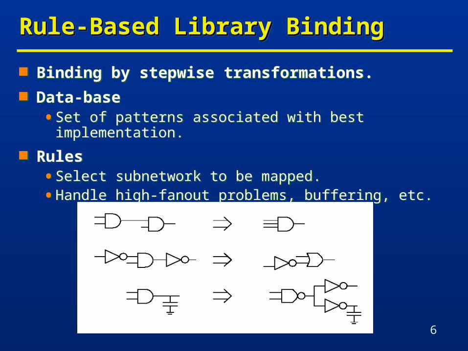
Binding by stepwise transformations. Data-base
• Set of patterns associated with best implementation.
Rules• Select subnetwork to be mapped.
• Handle high-fanout problems, buffering, etc.
Binding by stepwise transformations. Data-base
• Set of patterns associated with best implementation.
Rules• Select subnetwork to be mapped.
• Handle high-fanout problems, buffering, etc.
7
Rule-Based Library BindingRule-Based Library BindingRule-Based Library BindingRule-Based Library Binding
Execution of rules follows a priority scheme. Search for a sequence of transformations. A greedy search is a sequence of rules each decreasing cost. Search space
• Breadth (options at each step).
• Depth (look-ahead). Meta-rules determine dynamically breadth and depth. Advantages
• Applicable to all kinds of libraries. Disadvantages
• Large rule data-base• Completeness issue.
• Data-base updates.

8
Algorithms for Library BindingAlgorithms for Library BindingAlgorithms for Library BindingAlgorithms for Library Binding
Mainly for single-output combinational cells. Fast and efficient
• Quality comparable to rule-based systems.
Library description/update is simple• Each cell modeled by its function or equivalent pattern.
Involves two steps• Matching
• A cell matches a subnetwork if their terminal behavior is the same.
• Input-variable assignment problem.
• Covering• A cover of an unbound network is a partition into subnetworks
which can be replaced by library cells.
9
MatchingMatchingMatchingMatching
Given two single-output combinational functions f(x) and g(x) with same number of support variables.
f matches g if there exists a permutation P such that f(x) = g(P x).
Example• f = ab + c ; g = p + qr.
• By assigning {q, r, p} to {a, b, c}, f is equal to g.
• f and g have a Boolean match.
• By representing functions f and g by their AND-OR decomposition graphs, f and g have a structural match since their graphs are isomorphic.
10
AssumptionsAssumptionsAssumptionsAssumptions
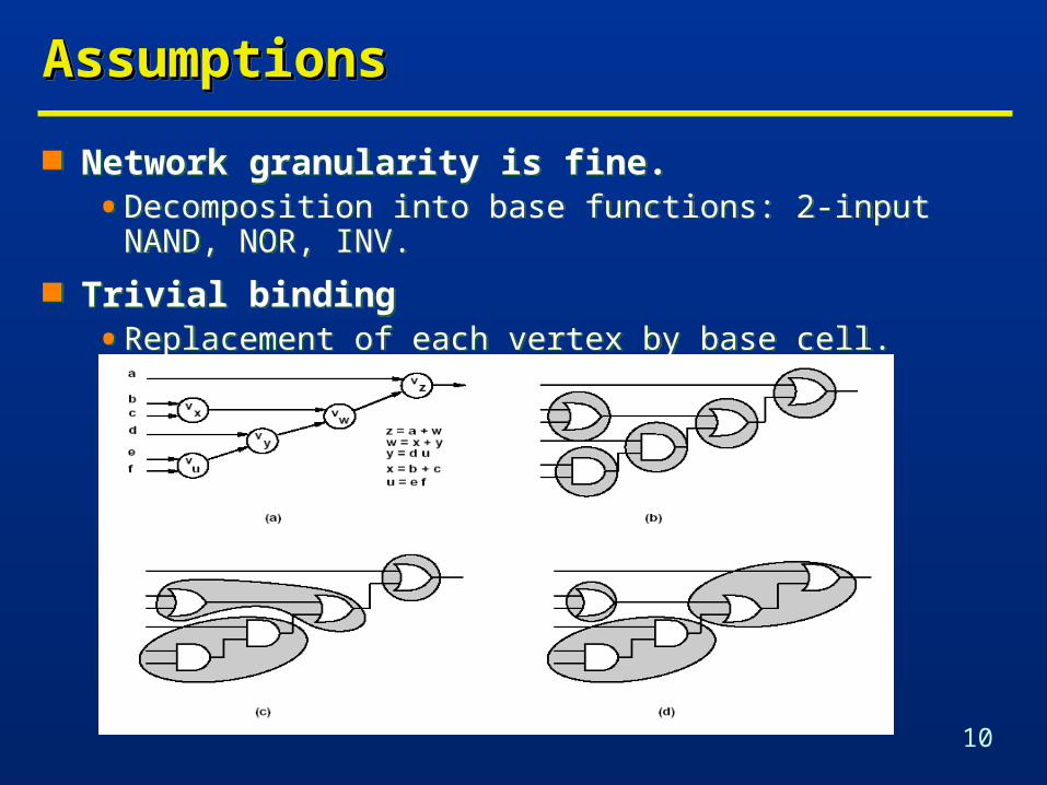
Network granularity is fine.• Decomposition into base functions: 2-input NAND, NOR, INV.
Trivial binding• Replacement of each vertex by base cell.
Network granularity is fine.• Decomposition into base functions: 2-input NAND, NOR, INV.
Trivial binding• Replacement of each vertex by base cell.
11
Example …Example …Example …Example …

12
… … ExampleExample… … ExampleExample
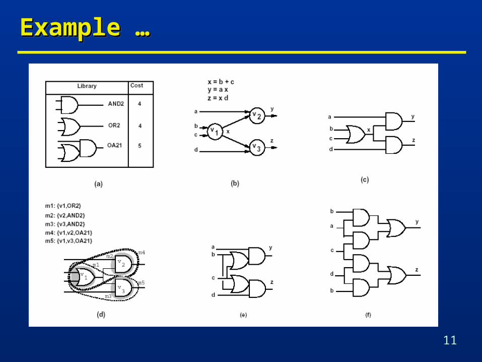
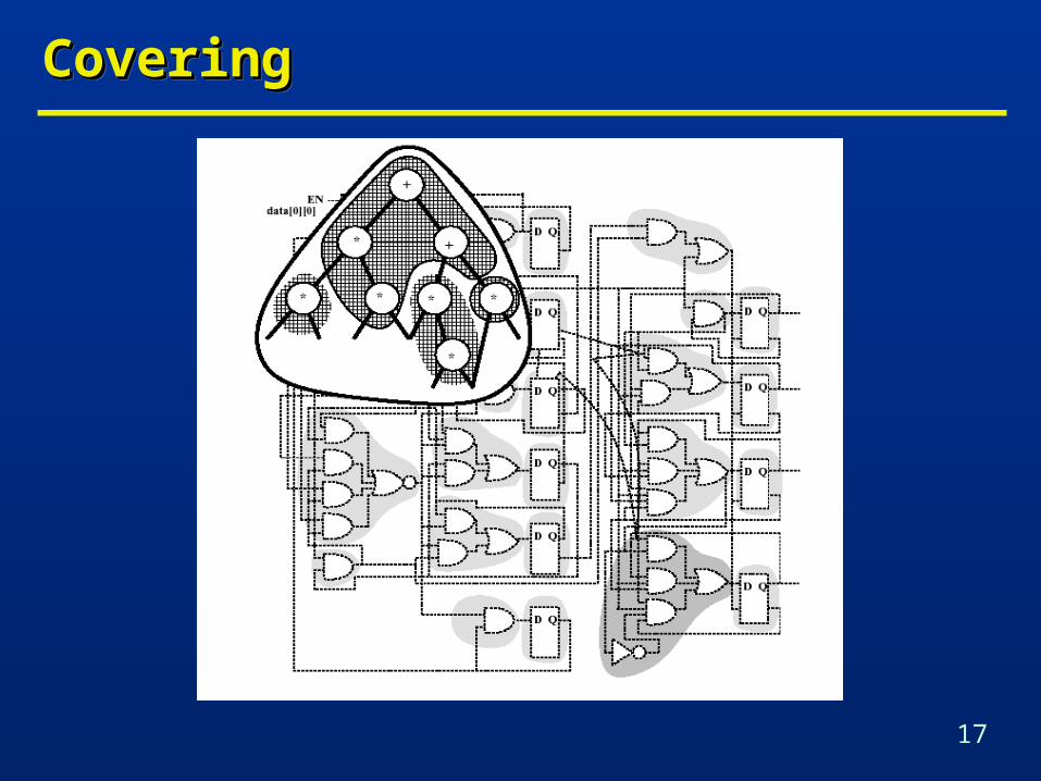
Vertex covering• Covering v1: (m1 +m4 +m5).
• Covering v2: (m2 +m4).
• Covering v3: (m3 +m5).
Input compatibility• Match m2 requires m1: (m2’ +m1).
• Match m3 requires m1: (m3’ +m1).
Overall binate clause• (m1 +m4 +m5)(m2 +m4)(m3 +m5)
(m2’ +m1)(m3’ +m1) = 1
Optimum solution: m1’m2’m3’m4m5• Cost=10
Vertex covering• Covering v1: (m1 +m4 +m5).
• Covering v2: (m2 +m4).
• Covering v3: (m3 +m5).
Input compatibility• Match m2 requires m1: (m2’ +m1).
• Match m3 requires m1: (m3’ +m1).
Overall binate clause• (m1 +m4 +m5)(m2 +m4)(m3 +m5)
(m2’ +m1)(m3’ +m1) = 1
Optimum solution: m1’m2’m3’m4m5• Cost=10

13
Heuristic AlgorithmsHeuristic AlgorithmsHeuristic AlgorithmsHeuristic Algorithms
To render covering problem tractable, network is decomposed and partitioned.
Decomposition• Cast network and library in standard form.
• Decompose into base functions.
• Example: NAND2 and INV.
• Guarantees that each vertex is covered by at least one match.
Partitioning• Break network into cones called subject graphs.
• Reduce to many multi-input single-output subnetworks.
Covering• Cover each subnetwork by library cells.
14
PartitioningPartitioningPartitioningPartitioning
Rationale for partitioning• Size of each covering problem is smaller.
• Covering problem becomes tractable.
Used to isolate combinational portions from sequential elements and I/Os.
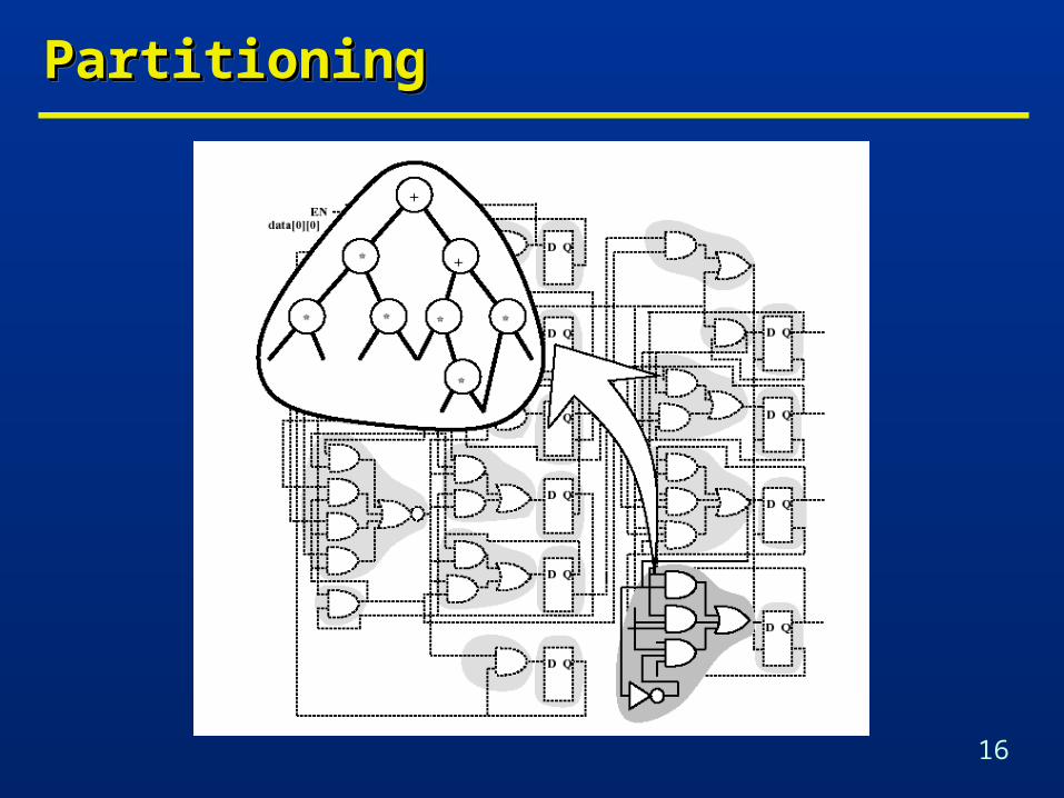
Partitioning of combinational circuits• Mark vertices with multiple fanout.
• Edges whose tails are marked vertices define partition boundary.
Rationale for partitioning• Size of each covering problem is smaller.
• Covering problem becomes tractable.
Used to isolate combinational portions from sequential elements and I/Os.
Partitioning of combinational circuits• Mark vertices with multiple fanout.
• Edges whose tails are marked vertices define partition boundary.

15
DecompositionDecompositionDecompositionDecomposition
16
PartitioningPartitioningPartitioningPartitioning
17
CoveringCoveringCoveringCovering
18
MatchingMatchingMatchingMatching
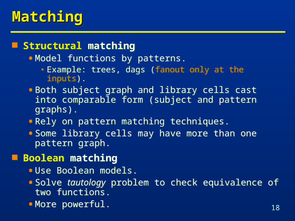
Structural matching• Model functions by patterns.
• Example: trees, dags (fanout only at the inputs).
• Both subject graph and library cells cast into comparable form (subject and pattern graphs).
• Rely on pattern matching techniques.
• Some library cells may have more than one pattern graph.
Boolean matching• Use Boolean models.
• Solve tautology problem to check equivalence of two functions.
• More powerful.
19
Boolean versus Structural MatchingBoolean versus Structural MatchingBoolean versus Structural MatchingBoolean versus Structural Matching
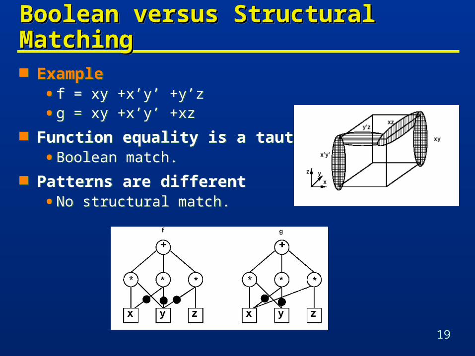
Example• f = xy +x’y’ +y’z
• g = xy +x’y’ +xz
Function equality is a tautology• Boolean match.
Patterns are different• No structural match.
Example• f = xy +x’y’ +y’z
• g = xy +x’y’ +xz
Function equality is a tautology• Boolean match.
Patterns are different• No structural match.

20
Structural Matching and CoveringStructural Matching and CoveringStructural Matching and CoveringStructural Matching and Covering
Expression patterns• Represented by dags using a
decomposition of 2-inp NAND and INV.
Identify pattern dags in network• Matching by sub-graph isomorphism.
Simplification• Use tree patterns.
• Most library cells can be represented as trees.
• Tree matching & tree covering is linear.
Expression patterns• Represented by dags using a
decomposition of 2-inp NAND and INV.
Identify pattern dags in network• Matching by sub-graph isomorphism.
Simplification• Use tree patterns.
• Most library cells can be represented as trees.
• Tree matching & tree covering is linear. F = a b c d
F = a b c d
F = a b F = a b
21
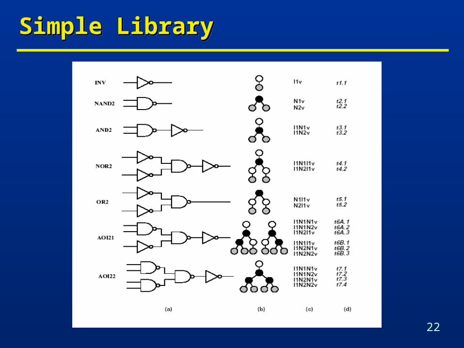
Tree-Based Matching …Tree-Based Matching …Tree-Based Matching …Tree-Based Matching …
Network• Partitioned and decomposed
• NOR2 (or NAND2) + INV.• Generic base functions.
• Each partition called Subject tree.
Library• Represented by trees.
• Possibly more than one tree per cell.
• Pattern recognition• Simple binary tree match.• Aho-Corasick automaton.
Network• Partitioned and decomposed
• NOR2 (or NAND2) + INV.• Generic base functions.
• Each partition called Subject tree.
Library• Represented by trees.
• Possibly more than one tree per cell.
• Pattern recognition• Simple binary tree match.• Aho-Corasick automaton.
22
Simple LibrarySimple LibrarySimple LibrarySimple Library
23
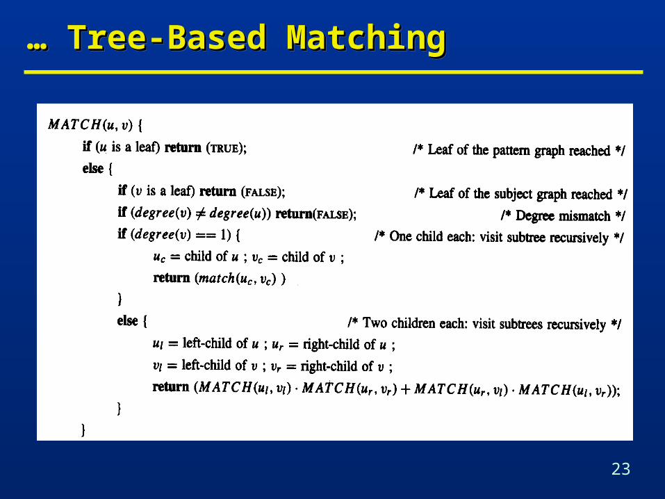
… … Tree-Based MatchingTree-Based Matching… … Tree-Based MatchingTree-Based Matching

24
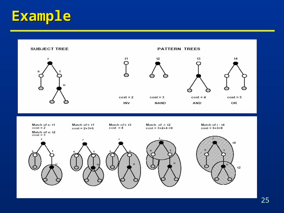
Tree-Based CoveringTree-Based CoveringTree-Based CoveringTree-Based Covering
Dynamic programming• Visit subject tree bottom-up.
At each vertex attempt to match• Locally rooted subtree.• Check all library cells for a match.
Optimum solution for the subtree.
Dynamic programming• Visit subject tree bottom-up.
At each vertex attempt to match• Locally rooted subtree.• Check all library cells for a match.
Optimum solution for the subtree.
25
ExampleExampleExampleExample
26
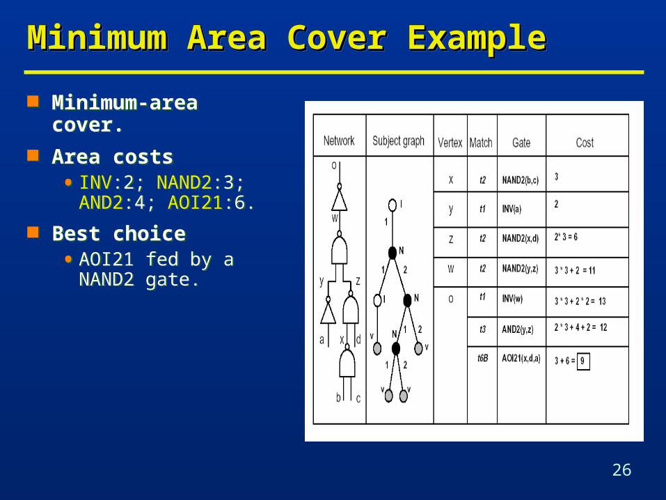
Minimum Area Cover ExampleMinimum Area Cover ExampleMinimum Area Cover ExampleMinimum Area Cover Example
Minimum-area cover. Area costs
• INV:2; NAND2:3; AND2:4; AOI21:6.
Best choice• AOI21 fed by a NAND2
gate.
Minimum-area cover. Area costs
• INV:2; NAND2:3; AND2:4; AOI21:6.
Best choice• AOI21 fed by a NAND2
gate.
27
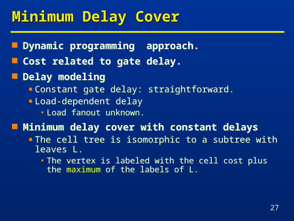
Minimum Delay CoverMinimum Delay CoverMinimum Delay CoverMinimum Delay Cover
Dynamic programming approach. Cost related to gate delay. Delay modeling
• Constant gate delay: straightforward.
• Load-dependent delay• Load fanout unknown.
Minimum delay cover with constant delays• The cell tree is isomorphic to a subtree with leaves L.
• The vertex is labeled with the cell cost plus the maximum of the labels of L.
28
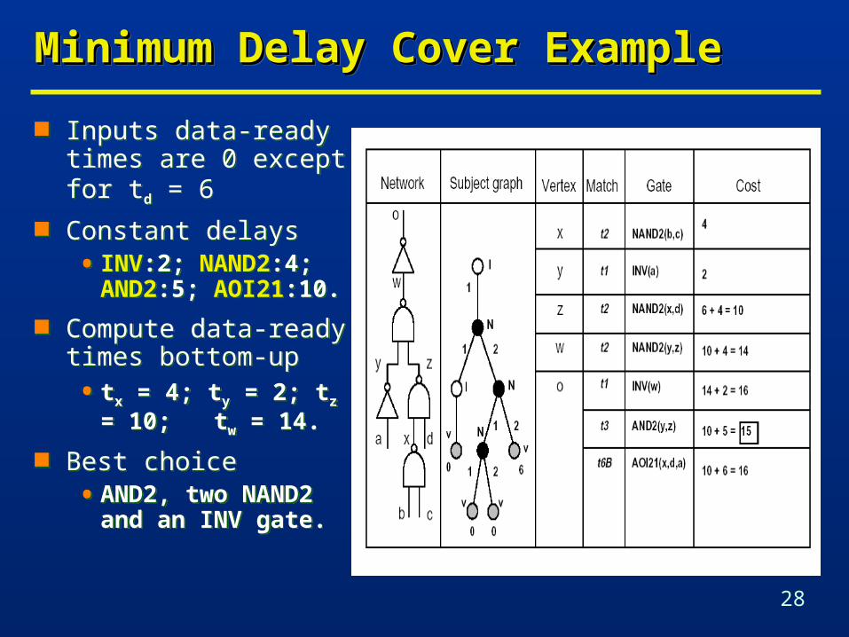
Minimum Delay Cover ExampleMinimum Delay Cover ExampleMinimum Delay Cover ExampleMinimum Delay Cover Example
Inputs data-ready times are 0 except for td = 6
Constant delays• INV:2; NAND2:4;
AND2:5; AOI21:10.
Compute data-ready times bottom-up
• tx = 4; ty = 2; tz = 10; tw = 14.
Best choice• AND2, two NAND2
and an INV gate.
Inputs data-ready times are 0 except for td = 6
Constant delays• INV:2; NAND2:4;
AND2:5; AOI21:10.
Compute data-ready times bottom-up
• tx = 4; ty = 2; tz = 10; tw = 14.
Best choice• AND2, two NAND2
and an INV gate.
29
Minimum Delay CoverMinimum Delay CoverLoad-Dependent DelaysLoad-Dependent DelaysMinimum Delay CoverMinimum Delay CoverLoad-Dependent DelaysLoad-Dependent Delays
Model• For most libraries, input capacitances are a finite small set.
• Label each vertex with all possible load values.
Dynamic programming approach• Compute an array of solutions for each vertex corresponding
to different loads.
• For each match, arrival time is computed for each load value.
• For each input to a matching cell the best match for the given load is selected.
Optimum solution, when all possible loads are considered.

30
ExampleExampleExampleExample
Inputs data-ready times are 0 except for td = 6
Load-dependent delays
• INV:1+l; NAND2:3+l; AND2:4+l; AOI21:9+l; SINV:1+0.5l.
Loads
• INV:1; NAND2:1; AND2:1; AOI21:1; SINV:2.
Assume output load is 1
• Same solution as before. Assume output load is 5
• Solution uses SINV cell.
Inputs data-ready times are 0 except for td = 6
Load-dependent delays
• INV:1+l; NAND2:3+l; AND2:4+l; AOI21:9+l; SINV:1+0.5l.
Loads
• INV:1; NAND2:1; AND2:1; AOI21:1; SINV:2.
Assume output load is 1
• Same solution as before. Assume output load is 5
• Solution uses SINV cell.
31
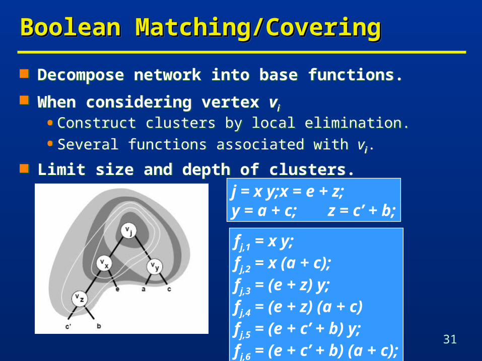
Boolean Matching/CoveringBoolean Matching/CoveringBoolean Matching/CoveringBoolean Matching/Covering
Decompose network into base functions.
When considering vertex vi
• Construct clusters by local elimination.
• Several functions associated with vi.
Limit size and depth of clusters.
Decompose network into base functions.
When considering vertex vi
• Construct clusters by local elimination.
• Several functions associated with vi.
Limit size and depth of clusters.j = x y; x = e + z;y = a + c; z = c’ + b;
fj,1 = x y;fj,2 = x (a + c);fj,3 = (e + z) y;fj,4 = (e + z) (a + c)fj,5 = (e + c’ + b) y;fj,6 = (e + c’ + b) (a + c);
32
Boolean Matching: P-EquivalenceBoolean Matching: P-EquivalenceBoolean Matching: P-EquivalenceBoolean Matching: P-Equivalence
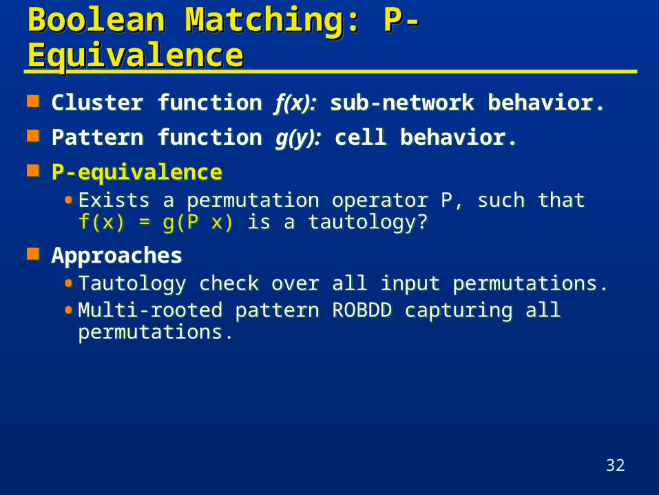
Cluster function f(x): sub-network behavior. Pattern function g(y): cell behavior. P-equivalence
• Exists a permutation operator P, such that f(x) = g(P x) is a tautology?
Approaches• Tautology check over all input permutations.
• Multi-rooted pattern ROBDD capturing all permutations.
Cluster function f(x): sub-network behavior. Pattern function g(y): cell behavior. P-equivalence
• Exists a permutation operator P, such that f(x) = g(P x) is a tautology?
Approaches• Tautology check over all input permutations.
• Multi-rooted pattern ROBDD capturing all permutations.
33
Signatures and Filters …Signatures and Filters …Signatures and Filters …Signatures and Filters …
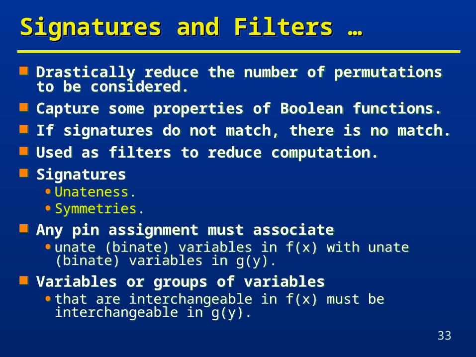
Drastically reduce the number of permutations to be considered.
Capture some properties of Boolean functions. If signatures do not match, there is no match. Used as filters to reduce computation. Signatures
• Unateness.• Symmetries.
Any pin assignment must associate• unate (binate) variables in f(x) with unate (binate) variables in
g(y). Variables or groups of variables
• that are interchangeable in f(x) must be interchangeable in g(y).

34
… … Signatures and Filters …Signatures and Filters …… … Signatures and Filters …Signatures and Filters …
Cluster and pattern functions must have the same number of unate and binate variables to match.
If there are b binate variables, un upper bound on number of variable permutations is b! (n-b)!• (instead of n!)
Example• g = s1 s2 a + s1 s2’ b + s1’ s3 c + s1’s3’ d.
• n=7 variables; 4 unate and 3 binate.
• Only 3! 4! = 144 variable orders and corresponding OBDDs. need to be considered in worst case.
• Compare this with overall number of permutations• 7!=5040
35
… … Signatures and Filters …Signatures and Filters …… … Signatures and Filters …Signatures and Filters …
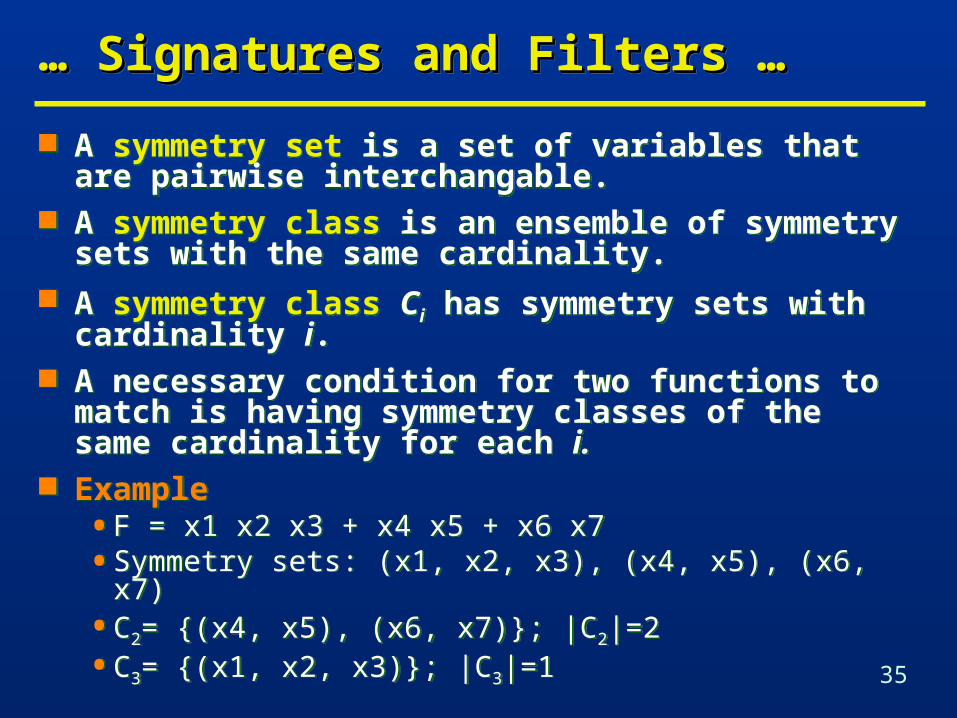
A symmetry set is a set of variables that are pairwise interchangable.
A symmetry class is an ensemble of symmetry sets with the same cardinality.
A symmetry class Ci has symmetry sets with cardinality i.
A necessary condition for two functions to match is having symmetry classes of the same cardinality for each i.
Example• F = x1 x2 x3 + x4 x5 + x6 x7• Symmetry sets: (x1, x2, x3), (x4, x5), (x6, x7)• C2= {(x4, x5), (x6, x7)}; |C2|=2• C3= {(x1, x2, x3)}; |C3|=1
36
… … Signatures and FiltersSignatures and Filters… … Signatures and FiltersSignatures and Filters
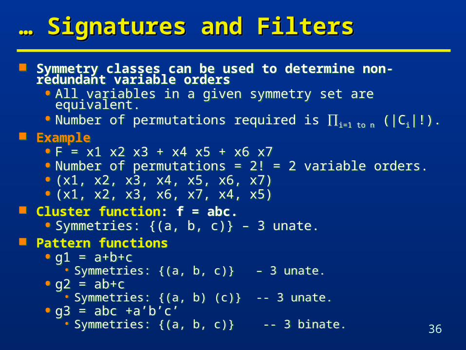
Symmetry classes can be used to determine non-redundant variable orders• All variables in a given symmetry set are equivalent.• Number of permutations required is i=1 to n (|Ci|!).
Example• F = x1 x2 x3 + x4 x5 + x6 x7• Number of permutations = 2! = 2 variable orders.• (x1, x2, x3, x4, x5, x6, x7)• (x1, x2, x3, x6, x7, x4, x5)
Cluster function: f = abc.• Symmetries: {(a, b, c)} – 3 unate.
Pattern functions• g1 = a+b+c
• Symmetries: {(a, b, c)} – 3 unate.• g2 = ab+c
• Symmetries: {(a, b) (c)} -- 3 unate.• g3 = abc +a’b’c’
• Symmetries: {(a, b, c)} -- 3 binate.