Code-to-Code Comparison of CFD/CSD Simulation for a Helicopter Rotor in Forward Flight

Jasim Ahmad∗ Robert T. Biedron†

NASA Ames Research Center, Moffet Field, CA 94035 NASA Langley Research Center, Hampton, VA 23681

AbstractTwo unsteady Reynolds-averaged Navier-Stokes solvers are used to compute the rotor airloads on the UH-60A

rotorcraft at several flight conditions across the flight envelope. One code, OVERFLOW, solves the flow equationsusing either structured grids, or a combination of structured and Cartesian grids. The other solver, FUN3D, usesunstructured grids. Both flow solvers are coupled to the same rotorcraft comprehensive code (CAMRAD II) inorder to account for trim and aeroelastic deflections, and both utilize the same loose coupling scheme to transferdata between the flow solver and the comprehensive code. In the process of performing the code-to-code compar-ison, several small but important details are examined that may sometimes be overlooked when comparing resultsfrom rotorcraft simulations using different codes. Computed normal force, pitching moment, and chord force arecompared between codes, and also with flight data.

Nomenclature

αs shaft angle of attack [◦]

β side slip angle (+ nose left) [◦]

µ advance ratio, M/Mtip

Ψ rotor azimuth [◦]

ρ density [slugs/ft3]

σ rotor solidity, nc/πR (0.0826)

a freestream speed of sound [ft/s]

c local chord [ft]

CT thrust coefficient [lb]

M freestream Mach number

M2Cc sectional chord force coefficient, F/( 12ρa

2c)

M2Cm sectional pitch moment coefficient, PM/( 12ρa

2c2)

M2Cn sectional normal force coefficient, N/( 12ρa

2c)

Mtip tip Mach number

n number of rotor blades (4)

R blade radius (26.833) [ft]

r radial coordinate [ft]

CAMRAD II Comprehensive Analytical Model of Rotor-craft Aerodynamics and Dynamics II

F sectional chord force [lb]

N sectional normal force [lb]

PM sectional pitch moment, [ft-lb]

IntroductionThe analysis of rotorcraft aerodynamics is quite challenging due to the coupling between the structural deformations

of the blades and the complex flowfield. The blade motions are required to either trim the vehicle in level flight or to effecta change in a maneuver. To model aerodynamics and structural dynamics in the analysis of rotorcraft systems, a numberof ‘comprehensive codes’ have been developed. In order to perform the analysis of these systems in a timely manner,comprehensive codes usually employ simplified methods or models within each of the various analysis tasks. For example,nonlinear beam models are used to model the structural dynamics of the blades rather than a more complete finite-elementmodel. For aerodynamic analysis, lifting-line models supplemented by two-dimensional airfoil lookup tables and wakemodels are often used. While a nonlinear beam is usually a good model for a long, slender rotor blade, for many flightconditions the simpler aerodynamics models are found to lack sufficient fidelity. To overcome the aerodynamic modeldeficiencies, the idea of correcting comprehensive codes with input from Computational Fluid Dynamics (CFD) codes iswidely used.1–4 The idea is to replace, through an iterative procedure, the aerodynamics computed by the comprehensivecode with the aerodynamics computed by the CFD code, while retaining all the other analysis capabilities of the com-prehensive code. At the same time, the effects of the structural dynamics of the blades, as well as the trim of the rotor,are brought into the CFD simulation. In this context, the primary contribution of the comprehensive code is to provide

∗Aerospace Engineer†Senior Research Scientist, Senior Member AIAAThis material is declared a work of the U.S. Government and is not subject to copyright protection in the United States.

1

American Institute of Aeronautics and Astronautics

a Computational Structural Dynamics (CSD) model and a mechanism for trim. The terms comprehensive code and CSDcode are used interchangeably in the remainder of the paper.

Under the NASA Subsonic Rotary Wing Project two general-purpose Reynolds Averaged Navier Stokes (RANS)solvers, OVERFLOW5 and FUN3D6 are being modified for and applied to a range of rotorcraft problems. The goal isto produce validated, high-fidelity tools for analysis and design. The two codes share a common file interface for couplingwith CSD codes. The purpose of this paper is to perform a detailed comparison of the computed rotor airloads from thesetwo CFD solvers, both coupled to the same CSD code, CAMRAD II.7 The computations will be performed for severalcases of interest for the UH-60A rotorcraft. The UH-60A is an excellent configuration for CFD/CSD validation, as anextensive set of flight-test measurements of aerodynamic and structural loads is available in the UH-60A database.8, 9

The purpose of performing a detailed code-to-code comparison, along with comparison of computed results with flight-test data, is to validate both codes in depth. In addition, we will examine some details of the coupling process that, whileimportant, are often overlooked or go unreported. By utilizing the same CSD solver (and the same inputs to the CSDsolver) for both CFD codes, any observed differences are attributed to the CFD side of the coupled simulations.

CFD CodesOVERFLOW and FUN3D have had a long history of development. The codes have a number of common attributes,

though they utilize distinctly different computational algorithms. OVERFLOW is a Reynolds-averaged Navier-Stokes(RANS) code that uses an overset structured/Cartesian grid system while FUN3D is an unstructured RANS solver that canoptionally utilize overset (unstructured) grids. These widely-used codes have very general capabilities for accommodatingmoving and deforming bodies, and as such are very suitable for rotorcraft simulations. Of the two, OVERFLOW has beenused more extensively for rotorcraft analysis. Both codes have interfaces with CAMRAD II (and other rotorcraft analysiscodes) to provide blade deformation and trim based on CSD computation.

OVERFLOW is a finite-difference, node-based solver. User-supplied, body-fitted structured grids are employed nearsolid surfaces, with automatically-generated background Cartesian grids filling the remainder of the computational do-main. Higher-order spatial differences, up to 5th order, are available for interior points. Physical boundary conditions areimplemented with reduced order. The code has several upwind flux schemes to improve the numerical accuracy for highspeed applications as well as for vortex dominated flows. The results presented here were obtained using one of the HLL10

family of upwind approximate-Riemann flux algorithms, namely, the contact-preserving HLLC variant,11 with nominally5th order accuracy in space for the inviscid fluxes. Reference 5 provides details of these algorithms. To advance the so-lution in time, an implicit, second-order backward difference scheme is used in which the nonlinear system of equationsis linearized at each time step. In this study, the resulting system of linear equations is solved using symmetric successiveoverrelaxation (SSOR), which eliminates factorization errors at the expense of more computational work and memory pertime step. Within OVERFLOW, several time-stepping schemes are available, including dual-time schemes. This studyused Newton iteration scheme. For this simulation, OVERFLOW used anywhere between 15 to 35 subiterations at eachtime step. A number of turbulence models are available in OVERFLOW. Here, the standard one-equation model of Spalartand Allmaras12 is utilized. For inter-grid communications between overset meshes, OVERFLOW can use either Pegasusor Domain Connectivity Function (DCF) using the X-Rays method of hole cutting.

FUN3D is a finite volume, node-based solver with 2nd order spatial accuracy. The code utilizes unstructured grids,which may be comprised of tetrahedral, prismatic, hexahedral, or pyramidal cells. Typical grids utilize prisms near solidsurfaces and tetrahedra to fill the remainder of the computational domain. FUN3D also has a number of flux functionsavailable. In this study, the standard Roe scheme13 is employed, with a least-squares approach used to evaluate the gradientsneeded for second-order reconstruction of the inviscid fluxes. Viscous terms are evaluated with second-order accuracyusing gradients computed using the Green-Gauss theorem. For non-tetrahedral meshes, the Green-Gauss gradients arecombined with edge-based gradients to avoid odd-even decoupling. In this approach, the full viscous terms are retained,i.e., no thin-layer approximations are made. The Spalart-Allmaras turbulence model is also used for the FUN3D resultspresented here. To advance the solution in time, an implicit, dual-time stepping scheme is used. The nonlinear equationsare linearized at each time step, with subiterations used to iteratively solve the nonlinear system. A point Gauss-Seidelscheme is used to solve the resulting linear system of equations at each subiteration step. Within FUN3D, the iterativeor pseudo-time step is based on a constant CFL number rather than the physical time step. The particular scheme usedin this study utilizes backward differences in time and although formally second-order accurate, has a smaller leading-order truncation error than the standard second-order backward difference scheme.14, 15 FUN3D can utilize either a fixednumber of subiterations per step, or can use an estimate of the temporal error to determine a suitable level of subiterationconvergence. The latter method is employed here. Subiterations are terminated when the subiteration residual (i.e., the errorin solving the nonlinear system of equations) drops to less than one percent of the temporal error estimate, or a maximumof 40 subiterations are performed. The goal is to ensure that the error in solving the nonlinear system of equations ateach time step is held below the error associated with the temporal discretization. This allows the design order of thetime-advancement scheme to be maintained. For the overset meshes needed for rotorcraft simulations, the DiRTlib16 and

2

American Institute of Aeronautics and Astronautics

SUGGAR++17 codes are used in conjunction with FUN3D to facilitate communication between disparate zones in themesh.

Fluid/Structural CouplingThe rotorcraft CSD code used for this study is CAMRAD II.7 The aerodynamics modules within CAMRAD II are based

on lifting-line models utilizing airfoil tables, coupled with wake models. Within CAMRAD II, each blade is structurallymodeled as a set of nonlinear beam elements. In addition to the structural dynamics modeling, CAMRAD II offers a trimcapability. For the UH-60A simulations in this paper, a three-degree-of-freedom trim is utilized, with the solidity-weightedthrust coefficient, pitching moment, and rolling moment specified as trim targets within CAMRAD II. In turn, CAMRADII provides the collective pitch, longitudinal cyclic, and lateral cyclic pitch angles.

The goal of the loose coupling approach is to correct the low-order lifting-line aerodynamics of the CSD code withthe higher-fidelity Navier-Stokes aerodynamics of the CFD code. In the loose coupling approach, shown schematicallyin Figure 1, quarter-chord (c/4) blade motion data from the CSD solver (upper red box in the figure) and quarter-chordaerodynamic force and moment (F/M) data from the CFD solver (lower red box) are exchanged at periodic intervals,for example, once per revolution or more generally once per integer multiple of the blade passage. In a typical coupledsimulation, the initial execution of the CFD code is carried out for one or two complete rotor revolutions, using bladedeformations from a trimmed CAMRAD II solution with unmodified lifting-line (superscript LL Fig. 1) in aerodynamics.In subsequent coupling cycles, the flow solver is run for one-half revolution between coupling cycles (full revolution forsome cases). At each coupling step, rotor loads from CFD are provided to CAMRAD II and in turn, CAMRAD II uses thisCFD load to make a correction to its own lifting-line aerodynamics to retrim the rotor. At convergence, the CFD airloadsfully replace comprehensive analysis airloads. The coupled FUN3D/CAMRAD and OVERFLOW/CAMRAD systems aretied together by separate interface codes that perform data translation between CFD and CSD. C-Shell scripts are used tomanage the execution of the various codes, and to provide restart, post-processing, and archiving functions. FUN3D andOVERFLOW utilize their own shell scripts, although the fundamental input and output are common to both CFD codes.

Geometrical ConsiderationsReference Blade Geometry

For the computed results presented below, both CFD solvers have utilized independently-created grids that define therotor blade. For each solver, one reference blade grid is created, and that reference grid is replicated and positioned todefine the four-bladed UH-60A rotor. The question then arises, how different are these independently-generated reference-blade geometries? Differences in reference-blade geometry will obviously lead to differences in solutions between thetwo codes. Although we may not be able to assess the sensitivity of the solution to the geometry for both solvers, we canat least quantify the differences in the geometries themselves. The differences (δ) in the y and z coordinates of the tworeference-blade geometries are shown in Fig. 2. It is seen that maximum differences in the reference surfaces are generallyvery small, except in the region near the blade root. The actual blade surface was not defined in this region of the originalblade model provided by Sikorsky and so the required closure in this region was done differently in each case. Thesedifferences in the root region are believed not to have a significant impact on the computed results as the root loading isgenerally very small.

Blade Motion/Deformation Verification

When utilizing a coupled CFD/CSD approach there are relatively complex geometry manipulations, for both input andoutput, that must be done for each time step within the CFD solver. Blade deformations from CAMRAD II are givenas (x,y,z) deflections of the quarter chord along with Euler-angle rotations, as functions of span and rotor azimuth angle.These quarter-chord data, encapsulated in the upper red box of Fig. 1, are used by the CFD code to define the three-dimensional blade surface at each time step. The deformed blades are then rotated through the proper shaft azimuth angleto position each blade at the current instant of time. The deformations and Euler angles extracted from the CAMRAD IIsolution are contained in a ‘motion file’, which is in a common format utilized by both codes. To assess the differencesin the way both flow solvers process this deformation data, a verification test was performed in which both solvers weregiven the same grid and motion file, and then the blades were run through each solver, accessing only the blade motionroutines, without actually performing a flow solution. At selected points along the rotor disk, the deformed blade surfaceswere output from each solver and compared. Fig. 3 shows the comparison, at a rotor azimuth of 180◦, of the differencesin y and z, normalized by the rotor radius. Comparisons at other azimuthal angles are similar. It can be seen that given thesame grid and motion file, the two solvers produce virtually identical blade deformations. Maximum differences are on theorder of 10−5R - a few thousandths of an inch on the full scale UH-60A rotor. Thus, geometrical differences arising fromhow the blades are moved and deformed in each code will be negligible compared to differences that are inherent in theindependently-generated reference blade grids.

3

American Institute of Aeronautics and Astronautics

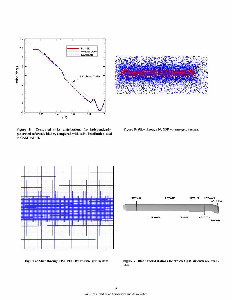
Twist Distribution

As implemented, coupling with CAMRAD II requires that forces and moments from CFD be defined in a local, section-aligned coordinate system for multiple radial stations along the blade. The CFD codes must therefore take the computedforces and moments, defined at discrete surface points, and resolve them into this local coordinate system. This processis encapsulated in the lower red box of Fig. 1. From a geometrical standpoint, this requires the flow solver to determinethe local quarter-chord location and local geometric twist, which in turn requires determination of the local leading andtrailing edges.

With a structured grid, this is a more straightforward operation than with an unstructured grid since the trailing edgeis always identified with a constant grid index and thus is explicitly set. With the trailing edge known, the leading edgecan then be defined by finding the point having the largest distance from the trailing edge (at the fixed radial location inquestion). In structured grids used for rotorcraft simulation, the chordwise grid lines are either collocated with, or parallelto, the radial stations at which sectional force and moment data are gathered for CAMRAD II. In an unstructured grid,there is often no grid point that lies at the trailing edge, and there is no convenient means (such as a constant grid index)to identify it a priori. Furthermore, grid points do not follow constant radial lines in an unstructured grid. Thus FUN3Dmust perform an intersection with the blade surface at each predetermined radial station. Within that intersected section,a search must be performed to find either the aft-most point in the blade section (for an idealized sharp trailing edge), oridentify two corner points and compute the midpoint between them (for the squared-off trailing edge typically found onproduction rotorcraft blades). Once the local trailing edge is found, the same process used by OVERFLOW to find theleading edge may be utilized.

To assess how closely the two CFD codes determine this local coordinate system, the resulting twist distributions inthe reference blade from both codes are shown in Fig. 4, together with the twist distribution specified in the CAMRAD IIinput. It is seen that the extracted twist from both codes is very nearly identical. The twist extracted from either grid differsslightly from the twist in CAMRAD II in the region 0.2 < r/R < 0.4; it is uncertain at this time which twist distributionis more faithful to the ’as-built’ twist. Although the CFD-computed twist distributions are shown only for the undeformedreference blade, the twist distribution must be recomputed for the current deformed blade shape at every time step todetermine the local section-aligned coordinate system in which loads are transferred back to CAMRAD II.

Grid Systems

The grid systems used to date by the two solvers are considerably different in size and type. The grid used for theFUN3D simulations consists of approximately 15 million nodes and 80 million cells. The number of unknowns in aFUN3D solution is proportional to the number of nodes. The grid is comprised of prismatic cells in the boundary-layerregion of the rotor blades, tetrahedral cells outside the boundary layer, and a small number of pyramidal cells in thetransition region between prismatic cells and tetrahedral cells. The background grid into which the rotor-blade gridsare overset is comprised entirely of tetrahedral cells. Near the outer boundary of the blade grids, the average spacingbetween nodes is approximately ten percent of the tip chord, though, due to the nature of the unstructured grid, this isonly an estimate. As can be seen in Fig. 5, the spacing in the (blue) background grid is more highly clustered in a regionsurrounding the rotor than away from it to better resolve the vortices shed by the blades. The unstructured grids used inthis study were generated using the advancing-layer and advancing-front grid generation software package.18

The grid used for the OVERFLOW simulations consists of approximately 71 million nodes with a nearly identicalnumber of cells. The number of unknowns in an OVERFLOW is also proportional to the number of nodes. The largenumber of grid points used in this simulation is in anticipation of running a future Detached Eddy Simulation (DES)that would also include fuselage. Although not shown, results from OVERFLOW were also obtained on a grid withapproximately 35 million nodes, and were virtually identical to those obtained using the larger mesh. The grid is comprisedof curvilinear, ‘O-mesh’ grids surrounding each blade, with the blade grids overset into automatically-generated Cartesiangrids. Each blade grid is comprised of three separate grids, one for the main portion of the blade, and separate cap gridsfor the tip and the root. The off-body Cartesian meshes are generated at various levels of resolution starting from ‘Level1’ near the blades, to ‘Level n’ in the farfield. For this study, the ‘Level 1’ grid spacing is set to ten percent of the tipchord, similar to that used in the unstructured FUN3D mesh. A slice through the structured/Cartesian grid system is shownin Fig. 6, where background grids through Level 5 are visible. The overset mesh used in OVERFLOW simulations aregenerated using Chimera Grid Tools (CGT).19 The CGT contains very efficient and modular grid scripting libraries usedfor grid manipulation, generation, reorganization, overset hole cutting surfaces, and producing flow solver input files. Thisscripting procedure allows production of high-quality surface meshes and subsequent volume meshes with a set of inputparameters. These scripts and input parameters enable modifications to the existing geometry and grid system to be madeautomatically and quickly.

4

American Institute of Aeronautics and Astronautics

Computational ResultsIn this section we compare the computational results obtained from OVERFLOW/CAMRAD and FUN3D/CAMRAD

with flight data. The focus is on rotor airloads. The UH-60A helicopter flight tests were part of the joint Army/NASA UH-60A Airloads Program and are widely used for validation of rotorcraft CFD simulation. In the flight test, the helicopter wasextensively instrumented with 242 pressure transducers at the nine radial locations shown in Fig. 7. Flight data rangingfrom high-torsional load maneuvers to very low-speed level flight were obtained. The details of all these flight conditionscan be found in Ref. 9. For this paper, two level flight cases were simulated.

When performing the computations, “best practices” were utilized for each code. In particular, the OVERFLOWsimulations were performed using a time step corresponding to 0.25◦ azimuth change, with a fixed number of subiterationsat each time step. FUN3D simulations were performed using a time step corresponding to 1.0◦ azimuth change, with avariable number of subiterations at each time step to attempt to drive the nonlinear residual to a small fraction (0.01) of thetemporal error.

In terms of computational resources, FUN3D simulations on a grid of 15 million nodes required 6.8 hours per halfrevolution (a typical interval between data exchanges with CAMRAD-II), using 289 Westmere cores of NASA’s Pleiadessupercomputer. For a grid of 71 million nodes, a half revolution in OVERFLOW required 5.5 hours using 984 Westmerecores on Pleiades. Converting the disparate grid sizes and CPUs utilized to a common basis, FUN3D required 131 CPUhours per million grid points for each half revolution, while OVERFLOW required 76 CPU hours per million grid pointsfor each half revolution.

The first comparison of results is shown for a flight condition denoted as Counter 9017 (C9017) in the UH-60A AirloadsDatabase. This condition is one of the most challenging level-flight conditions in the database, as it represents a high-thrustcondition (CT /σ = 0.129) at a moderate advance ratio (µ = 0.245). The high-thrust level is very close to the stallboundary and leads to dynamic stall at several locations on the retreating side of the rotor disk. The high loading for thislevel flight condition was achieved by flying at a high altitude.

Results are presented for normal force, pitching moment, chord force, and torsion moments. Fig. 8 shows the variationwith rotor azimuth angle of the flight data and computed results for a subset of these radial stations. The results arepresented in a triptych format which makes it easy to see the simultaneous effects of an “event”, such as dynamic stall, onall three quantities. In these plots, all harmonics are shown and means are removed from the data. The mean removal fromthe data for comparison is an accepted practice in order to compare oscillatory behavior of the load. This also removesknown uncertainty in the measured data, especially, the pressure transducers near the trailing edge. The pitching momentis difficult to measure due to sensitivity of pressure transducer performance. The dynamic stall cycle in a rotor flow canbe better examined from various plots when we look at the stall cycle in unconventional azimuthal scale of the rotor disk.This follows from the convention used by Bousman in his study of dynamic stall,20 where the starting azimuth is taken as135◦ instead of 0◦. This azimuth of 135◦ is midway through the second quadrant of the disk. This shift allows one to lookat the stall cycle in its entirety as one does not need to look back and forth at the fourth quadrant and the first quadrant asin the case of plots starting from 0◦.

In general the variations of rotor airloads with azimuthal angle are reasonably well predicted by both codes. At stationr/R = 0.865, near azimuth angles of 255◦ and 315◦, successive dynamic stall events are observed, wherein the normalforce drops sharply, chord force increases, and the pitching moment becomes much more negative. On the advancing sideat this radial station, a much more mild drop in normal and chord force, together with a slightly more nose-down pitchingmoment is observed near ψ = 55◦. These are indicative of a light stall, one that does not extend to the trailing edge.20 Itshould be noted that the chord force is taken as positive in the local “y” direction of the reference-blade coordinate system,which progresses from the trailing edge to the leading edge, as indicated in Fig. 2. Both simulations capture the doublestall event on the retreating side well, and both exhibit the light lift-stall on the advancing side. The stall events are similarin the two simulations, with some minor differences in the stall location and the magnitude of the forces and moments.

In Fig. 9, the computed and measured loads at all nine radial stations are averaged over 360◦ of rotor rotation to definethe mean sectional loads. The mean of the measured data for normal force and chord force at r/R = 0.400 clearly does notfollow the trend of the mean of the measured data at nearby stations. Similarly, the mean pitching moment in the measureddata at r/R = 0.865 seems unexpectedly different from neighboring radial stations. Except for a small difference in themean pitching moment at r/R = 0.865, the mean sectional loads from the two simulations are very nearly identical.However, the agreement between computation and flight for the mean normal force, and especially for mean pitchingmoment, is not satisfactory.

Some of the offsets in airload between flight and computation may be due to inconsistencies in the measurements,as discussed above. Therefore, to better assess how well the computational results capture the variation with azimuthalposition, Figures 10-12 qualitatively compare the normal force, pitching moment, and chord force, each with the respectivemean values removed, across the entire rotor disk. The two CFD/CSD simulations agree well with each other, and generallyagree well with the flight data. Both simulations miss the peak negative loading near the tip in the second quadrant of therotor disc. Both codes predict too large a chord force in the second quadrant, two thirds of the way out the span.

5

American Institute of Aeronautics and Astronautics

Some of the torsional moments are compared in Fig. 13 for this case. The torsional loads from the two simulationsare very similar to each other and generally follow the trend of the flight data. The OVERFLOW results tend to producesomewhat larger peak torsional moments, in slightly better agreement with the data. The flight data show successive peaksin the torsional moment in the first quadrant, particularly evident at r/R = 0.0466 and r/R = 0.500. Both computationsonly show a single peak. Likewise, successive troughs are seen in the flight data near ψ = 270◦, whereas both computationsexhibit only a single local minimum in that region.

The second comparison of results from the two codes is for the low-speed condition of flight counter C8513. Thislevel-flight conditions is not as severe as the high thrust case of C9017. It represents a Blade Vortex Interaction (BVI)condition with trim target of CT /σ = 0.087 at a moderate advance ratio (µ = 0.15). The flight data for this condition weretaken at a relatively large side-slip angle β = 7.71◦. This side-slip angle was used in the OVERFLOW simulations, butnot in the FUN3D simulations. To approximately compensate for this difference between the two simulations, the FUN3Dresults are shifted in azimuth (to the left) by 7.71◦. Since neither simulation included fuselage, this shift should yield thesame end result as if the correct side-slip had been used. The OVERFLOW and FUN3D results are close to each other,indicating that the rotor is trimmed to appropriate aerodynamic loads, despite the difference in side slip angles. Results areagain presented for normal force, pitching moment, and chord force. Fig. 14 shows the variation with rotor azimuth angleof the flight data and computed results. The BVI events at 90 degrees, and 270 degrees are reasonably captured, especially,large variation of the blade loading and phase on the advancing side and retreating side. The normal force and pitchingmoment comparison is noticeably better near the root region. The pitching moments are underpredicted near the tip. Thechord forces show different trend than the normal force and pitching moments which both simulations predict too high avalue near the root and too low a value near the tip.

Fig. 15 shows the computed and measured azimuthal average loads of all nine radial stations. Both FUN3D andOVERFLOW results are almost identical. However, the agreement between computation and flight for the mean chordforce, and the mean pitching moment is not satisfactory.

Fig. 16 shows the torsional moment variations for this low-speed case. The FUN3D results are again shifted to the leftin azimuth by 7.71◦ to account for β = 0◦ in the FUN3D simulation. The torsional loads computed by the two codes arevirtually indistinguishable. Comparison with flight data is not entirely satisfactory.

Finally we present the convergence of the loose coupling steps in Fig. 17 for C9017 and in Fig. 18 for C8513. Theconvergence is represented here with control angles measured at the pitch link, where θ0 is the collective angle, θ1c, andθ1s are the lateral and longitudinal cyclic pitch respectively. The dynamic stall case of C9017 needed more than 25 cyclesto reach a converged state. This is true for both codes although FUN3D was run only for 25 cycles. With FUN3D, theconvergence of all three control angles exhibited a lightly damped oscillation, and by 25 trim cycles, the peak-to-peakoscillations control angles were less than 0.25◦. The convergence of OVERFLOW was seemingly more rapid, althoughbetween trim cycles 20 and 30, oscillations on the order of 0.25◦ appeared and were then damped out. The large numberof coupling steps required for this high thrust condition makes this case computationally expensive. It would be interestingto see how this compares when one tries to simulate a maneuvering flight. In contrast, the simulation of C8513 trimmedin less than 10 cycles. For both flight counters, the OVERFLOW/CAMRAD-II and FUN3D/CAMRAD-II coupling yieldtrimmed control angles that differ by less than 0.50◦.

ConclusionsThe unstructured Navier-Stokes CFD code FUN3D and structured Navier-Stokes code OVERFLOW used the same

comprehensive code CAMRAD II in a loosely coupled manner that satisfactorily compared with the flight test data. TheFUN3D uses second-order spatial and time accuracy, while OVERFLOW uses mixed-order spatial accuracy with second-order time accuracy. The blade motion and grid deformation for both cases presented were properly verified to make surethat both of the codes solved the same problem. The challenging flight test case with multiple dynamic stall events isreasonably represented, although some obvious discrepancies of forces and moments were seen near the stall location,especially, for chord forces. However, the stall location seems to be well captured. The low-speed case of blade vortexinteraction compares well for both codes. For both codes, the loose coupling convergence to a trim state is expensive forthe dynamic stall case. The number of coupling steps needed for the BVI case is reasonably small.

AcknowledgmentsThe authors would like to thank Ms. Elizabeth Lee-Rausch of the Computational AeroSciences Branch at NASA

Langley Research Center for her many contributions to this work. The rotor-blade definitions were graciously provided byMr. T. Alan Egolf of the Sikorsky Aircraft Corporation. The authors would like to thank Dr. Pieter Buning for helpfuldiscussions regarding OVERFLOW. Finally, we would like thank Dr. Hyeonsoo Yeo of the U.S. Army AeroflightdynamicsDirectorate for providing the CAMRAD II input files.

6

American Institute of Aeronautics and Astronautics

References1Potsdam, M., Yeo, H., and Johnson, W., “Rotor Airloads Prediction Using Aerodynamic/Structural Coupling,” American Helicopter Society 60th

Annual Forum Proceedings, 2004.2Pahlke, K. and van der Wall, B., “Chimera simulations of multibladed rotors in high-speed forward flight with weak fluid-structure-coupling,”

Aerospace Science and Technology, Vol. 9, No. 5, 2005, pp. 379–389.3Lim, J. W. and Strawn, R. C., “Prediction of HART II Rotor BVI Loading and Wake System Using CFD/CSD Loose Coupling,” AIAA Paper

2007-1281, Jan. 2007.4Sankaran, V., Sitaraman, J., Wissink, A., Datta, A., Jayaraman, B., Potsdam, M., Mavriplis, D., Yang, Z., O’Brien, D., Saberi, H., Cheng, R.,

Hariharan, N., and Strawn, R., “Application of the Helios Computational Platform to Rotorcraft Flowfields,” AIAA Paper 2010-1230, Jan. 2010.5Nichols, R., Trammel, R., and Buning, P., “Solver and Turbulence Model Upgrades to OVERFLOW 2 for Unsteady and High-Speed Applications,”

AIAA Paper 2006-2824, June 2006.6Anderson, W. K. and Bonhaus, D. L., “An Implicit Upwind Algorithm for Computing Turbulent Flows on Unstructured Grids,” Computers and

Fluids, Vol. 23, No. 1, 1994, pp. 1–22.7Johnson, W., “Rotorcraft Aerodynamics Models for a Comprehensive Analysis,” American Helicopter Society 54th Annual Forum Proceedings,

1998.8Bondi, M. J. and Bjorkman, W. S., “Trends User’s Guide and Reference Manual,” NASA TM 108806, June 1994.9Bousman, W. G. and Kufeld, R. M., “UH-60A Airloads Catalog,” NASA TM 2005-212827, Aug. 2005.

10Harten, A., Lax, P. D., and van Leer, B., “On Upstream Differencing and Godunov-type Schemes for Hyperbolic Conservation Laws,” SIAMReview, Vol. 25, No. 1, 1983, pp. 35–61.

11Toro, E. F., Spruce, M., and Speares, W., “Restoration of the Contact Surface in the HLL Riemann Solver,” Shock Waves, Vol. 2, 1994, pp. 25–34.12Spalart, P. R. and Allmaras, S. R., “A One-Equation Turbulence Model for Aerodynamic Flows,” La Recherche Aerospatiale, No. 1, 1994,

pp. 5–21.13Roe, P. L., “Approximate Riemann Solvers, Parameter Vectors, and Difference Schemes,” Journal of Computational Physics, Vol. 43, 1981,

pp. 357–372.14Vatsa, V. and Carpenter, M. H., “Higher-Order Temporal Schemes with Error Controllers for Unsteady Navier-Stokes Equations,” AIAA Paper

2005-5245, June 2005.15Vatsa, V. N., Carpenter, M. H., and Lockard, D. P., “Re-evaluation of an Optimized Second Order Backward Difference (BDF2OPT) Scheme for

Unsteady Flow Applications,” AIAA Paper 2010-0122, Jan. 2010.16Noack, R. W., “DiRTlib: A Library to Add an Overset Capability to Your Flow Solver,” AIAA Paper 2005-5116, June 2005.17Noack, R. W., Bogar, D. A., Kunz, R. F., and Carrica, P. M., “SUGGAR++: An Improved General Overset Grid Assembly Capability,” AIAA

Paper 2009-3992, June 2009.18Prizadeh, S. Z., “Advanced Unstructured Grid Generation for Complex Aerodynamic Applications,” AIAA Journal, Vol. 48, No. 5, May 2010,

pp. 904–915.19Chan, W. M., “Enhancements to the Grid Generation Script Library and Post-Processing Utilities in Chimera Grid Tools,” Proceedings 9th

Symposium on Overset Composite Grid and Solution Technology, Oct. 2008.20Bousman, W. G., “A Qualitative Examination of Dynamic Stall from Flight Test Data,” American Helicopter Society 53th Annual Forum Pro-

ceedings, 1997.

7

American Institute of Aeronautics and Astronautics

Rotorcraft CSD CodeIter i = 0: F/M0 = F/MLL

0Iter i > 0: F/Mi = F/MLL

i + ∆F/Mi-1

∆F/Mi-1 = ∆F/Mi-2 + (F/MCFDi-1 - F/Mi-1)

Obtain Trimmed Control Settings For Rotor F/M

c/4 Motion - disp & rot

Move Grid + CFD Soln

F/M along c/4

F/M and TrimConverged?

no yesDone

F/M: CN, CM, CChord

Figure 1: Flow diagram for loose coupling between CFD and CSD codes; adapted from Reference 1.

Figure 2: Differences in independently-generated reference-bladegrids used in each solver.

Figure 3: Differences in blade deformation after motion through180◦ azimuth, using the identical structured/hexahedral reference-blade grid in each solver; identical motion files.

8

American Institute of Aeronautics and Astronautics

r/R

Tw

ist(

deg.

)

0 0.2 0.4 0.6 0.8 1-4

-2

0

2

4

6

8

10

12

FUN3DOVERFLOWCAMRAD

-160 Linear Twist

Figure 4: Computed twist distributions for independently-generated reference blades, compared with twist distribution usedin CAMRAD II.

Figure 5: Slice through FUN3D volume grid system.

Figure 6: Slice through OVERFLOW volume grid system. Figure 7: Blade radial stations for which flight airloads are avail-able.

9

American Institute of Aeronautics and Astronautics

Ψ, deg.135 180 225 270 315 360 405 450 495

-0.05

-0.04

-0.03

-0.02

-0.01

0

0.01

0.02

0.03

0.04M2Cm - mean

r/R = 0.400

135 180 225 270 315 0 45 90 135Ψ, deg.

135 180 225 270 315 360 405 450 495-0.3

-0.25

-0.2

-0.15

-0.1

-0.05

0

0.05

0.1

0.15

0.2

C9017FUN3DOVERFLOW

M2Cn - mean

135 180 225 270 315 0 45 90 135Ψ, deg.

135 180 225 270 315 360 405 450 495-0.04

-0.03

-0.02

-0.01

0

0.01

0.02

0.03M2Cc - mean

135 180 225 270 315 0 45 90 135

Ψ, deg.135 180 225 270 315 360 405 450 495

-0.05

-0.04

-0.03

-0.02

-0.01

0

0.01

0.02

0.03

0.04M2Cm - mean

r/R = 0.865

135 180 225 270 315 0 45 90 135Ψ, deg.

135 180 225 270 315 360 405 450 495-0.3

-0.25

-0.2

-0.15

-0.1

-0.05

0

0.05

0.1

0.15

0.2

C9017FUN3DOVERFLOW

M2Cn - mean

135 180 225 270 315 0 45 90 135Ψ, deg.

135 180 225 270 315 360 405 450 495-0.04

-0.03

-0.02

-0.01

0

0.01

0.02

0.03M2Cc - mean

135 180 225 270 315 0 45 90 135

Ψ, deg.135 180 225 270 315 360 405 450 495

-0.05

-0.04

-0.03

-0.02

-0.01

0

0.01

0.02

0.03

0.04M2Cm - mean

r/R = 0.990

135 180 225 270 315 0 45 90 135Ψ, deg.

135 180 225 270 315 360 405 450 495-0.3

-0.25

-0.2

-0.15

-0.1

-0.05

0

0.05

0.1

0.15

0.2

C9017FUN3DOVERFLOW

M2Cn - mean

135 180 225 270 315 0 45 90 135Ψ, deg.

135 180 225 270 315 360 405 450 495-0.04

-0.03

-0.02

-0.01

0

0.01

0.02

0.03M2Cc - mean

135 180 225 270 315 0 45 90 135

Figure 8: Comparison of computed and measured sectional airloads at r/R = 0.400, r/R = 0.865 and r/R=0.990, Counter 9017.

10

American Institute of Aeronautics and Astronautics

r/R0 0.2 0.4 0.6 0.8 1

-0.1

0

0.1

0.2

0.3

0.4C9017FUN3DOVERFLOW

Mean M 2Cn

r/R0 0.2 0.4 0.6 0.8 1

-0.1

-0.08

-0.06

-0.04

-0.02

0

0.02

0.04

Mean M 2Cc

r/R0 0.2 0.4 0.6 0.8 1

-0.04

-0.03

-0.02

-0.01

0

0.01

0.02Mean M 2Cm

Figure 9: Comparison of computed and measured mean (azimuthally averaged) sectional airloads, Counter 9017.

Figure 10: Comparison of computed and measured section normal force (mean removed), Counter 9017.

Figure 11: Comparison of computed and measured section pitching (mean removed), Counter 9017.

11

American Institute of Aeronautics and Astronautics

Figure 12: Comparison of computed and measured section chord force (mean removed), Counter 9017.

Ψ, deg

Tor

sion

Mom

ent-

Mea

n,in

-lb

0 90 180 270 360-10000

-5000

0

5000

10000

C9017FUN3DOVERFLOW

r/R = 0.0466

Ψ, deg

Tor

sion

Mom

ent-

Mea

n,in

-lb

0 90 180 270 360-10000

-5000

0

5000

10000r/R = 0.300

Ψ, deg

Tor

sion

Mom

ent-

Mea

n,in

-lb

0 90 180 270 360-10000

-5000

0

5000

10000r/R = 0.500

Ψ, deg

Tor

sion

Mom

ent-

Mea

n,in

-lb

0 90 180 270 360-10000

-5000

0

5000

10000r/R = 0.900

Figure 13: Comparison of computed and measured torsional moments (mean removed), Counter 9017.

12

American Institute of Aeronautics and Astronautics

Ψ, deg.0 45 90 135 180 225 270 315 360

-0.01

-0.005

0

0.005

0.01M2Cm - mean

r/R = 0.400

Ψ, deg.0 45 90 135 180 225 270 315 360

-0.1

-0.05

0

0.05

0.1

C8513OVERFLOWFUN3D

M2Cn - mean

Ψ, deg.0 45 90 135 180 225 270 315 360

-0.02

-0.01

0

0.01M2Cc - mean

Ψ, deg.0 45 90 135 180 225 270 315 360

-0.01

-0.005

0

0.005

0.01M2Cm - mean

r/R = 0.865

Ψ, deg.0 45 90 135 180 225 270 315 360

-0.1

-0.05

0

0.05

0.1

C8513OVERFLOWFUN3D

M2Cn - mean

Ψ, deg.0 45 90 135 180 225 270 315 360

-0.02

-0.01

0

0.01M2Cc - mean

Ψ, deg.0 45 90 135 180 225 270 315 360

-0.01

-0.005

0

0.005

0.01M2Cm - mean

r/R = 0.965

Ψ, deg.0 45 90 135 180 225 270 315 360

-0.1

-0.05

0

0.05

0.1

C8513OVERFLOWFUN3D

M2Cn - mean

Ψ, deg.0 45 90 135 180 225 270 315 360

-0.02

-0.01

0

0.01M2Cc - mean

Figure 14: Comparison of computed and measured sectional airloads at r/R = 0.400, r/R = 0.865 and r/R=0.965, Counter 8513.

13

American Institute of Aeronautics and Astronautics

r/R0 0.2 0.4 0.6 0.8 1

-0.1

0

0.1

0.2

0.3

0.4C8513FUN3DOVERFLOW

Mean M 2Cn

r/R0 0.2 0.4 0.6 0.8 1

-0.1

-0.08

-0.06

-0.04

-0.02

0

0.02

0.04

Mean M 2Cc

r/R0 0.2 0.4 0.6 0.8 1

-0.04

-0.03

-0.02

-0.01

0

0.01

0.02Mean M 2Cm

Figure 15: Comparison of computed and measured mean (azimuthally averaged) sectional airloads, Counter 8513.

Ψ, deg

Tor

sion

Mom

ent-

Mea

n,in

-lb

0 90 180 270 360-10000

-5000

0

5000

C8513FUN3DOVERFLOW

r/R = 0.0466

Ψ, deg

Tor

sion

Mom

ent-

Mea

n,in

-lb

0 90 180 270 360-10000

-5000

0

5000r/R = 0.300

Ψ, deg

Tor

sion

Mom

ent-

Mea

n,in

-lb

0 90 180 270 360-10000

-5000

0

5000r/R = 0.700

Ψ, deg

Tor

sion

Mom

ent-

Mea

n,in

-lb

0 90 180 270 360-10000

-5000

0

5000r/R = 0.900

Figure 16: Comparison of computed and measured torsional moments (mean removed), Counter 8513.

14

American Institute of Aeronautics and Astronautics

Coupling Cycle

The

ta0

The

ta1C

The

ta1S

0 5 10 15 20 25 30 35 4011.5

12.5

13.5

14.5

2

3

4

5

-10

-9

-8

-7

FUN3DOVERFLOW

Figure 17: Comparison of coupling convergence, Counter 9017.

Coupling Cycle

The

ta0

The

ta1C

The

ta1S

0 5 10 156

7

8

9

2

3

4

5

-6

-5

-4

-3

FUN3DOVERFLOW

Figure 18: Comparison of coupling convergence, Counter 8513.

15

American Institute of Aeronautics and Astronautics