Embed Size (px)
Citation preview

Coarse updating: Bertrand competition
Peter Eccles∗ Nora Wegner†
November 5, 2014
Abstract
In this paper we propose a theory of Bertrand competition where firms form beliefs
by considering only a subset of the available variables. This theory of coarse updat-
ing leads to equilibria where firms set prices according to constant mark-up strategies,
which is consistent with the evidence from survey data. It also can explain the high
price dispersion observed in practice without requiring an unreasonable level of cost dis-
persion. In general more sophisticated firms who consider all variables have incentives
to deviate from coarse equilibria. However we show that when costs are sufficiently
correlated, equilibria under coarse updating correspond to ε-equilibria under Bayesian
updating. Hence in this case even more sophisticated firms have little incentive to
deviate from coarse equilibria. Finally in the case of procurement auctions this theory
of coarse updating leads to a particularly simple estimation procedure where costs can
be recovered from pricing data using fewer observations than standard methods.
∗† Universidad Carlos III de Madrid, Department of Economics, C/Madrid 126, 28903 Getafe (Madrid),Spain. Email addresses: [email protected], [email protected]. We would like to thank oursupervisors Natalia Fabra and Angel Hernando-Veciana for their suggestions and advice.
1

1 Introduction
There is extensive empirical evidence that firms engage in mark-up pricing and set prices by
adding a constant percentage mark-up to their marginal cost. For example, when asked how
the price of their main UK product was determined, 44% of firms replied that direct cost
per unit plus a fixed percentage mark-up was an important or very important component of
their price-setting strategy (Greenslade & Parker (2010) and Greenslade & Parker (2012)).
Meanwhile a survey of German firms reported that firms take calculated unit costs as a
reference and then choose a mark-up based on market and competition conditions (Stahl
(2005)). Moreover in a survey of Italian firms 63% reported applying a mark-up to unit
variable costs (Fabiani et al. (2010)).
These surveys provide substantial evidence that mark-up pricing plays an important role
in pricing strategies, in particular when firms have market power. Moreover the mark-up
variable is extensively discussed in the business community and there is ample anecdotal
evidence that mark-up strategies play an important role in firms’ decision making. For
instance Rothkopf (1980) writes that discussions with the preparers of bids in industry do
not disclose a policy of systematically varying the multiple of an estimate that is bid as a
function of that estimate, which suggests that mark-up pricing is prevalent. Despite the
extensive evidence, the standard pricing model does not predict that firms bid according
to mark-up pricing. Indeed the standard model predicts that firms will vary their mark-up
according to their cost parameter, tending to bid a lower mark-up when their cost parameter
is higher.
In light of this shortcoming of the standard model, we build on the theory of cue competi-
tion developed in psychology and apply it to the pricing problem. This theory has several
advantages over alternative theories since it is (i) motivated by psychological evidence, (ii)
consistent with empirical findings and (iii) easy to recover costs from bids when firms compete
in procurement auctions. Building on the theory of cue competition developed in psychol-
ogy leads us to introduce a new assumption about how firms form beliefs, which we refer to
as coarse updating. The theory of coarse updating we consider assumes that firms do not
2

use information about the magnitude of their marginal cost when forming beliefs about the
expected quantity they will produce, and results in equilibria where firms use constant mark-
up strategies. Meanwhile in the case of procurement auctions the theory leads to a simple
procedure for estimating costs when the bids submitted are known. As well as capturing
the fact that firms bid according to constant mark-up strategies, this estimation procedure
requires less data than existing techniques, such as the procedure proposed by Campo et al.
(2003).
Generating the price dispersion observed in practice1 using the standard model typically
requires assuming an underlying cost distribution that is unreasonably dispersed and where
some firms set unreasonably high-markups. An et al. (2010) provide a solution for this prob-
lem, by considering an unknown number of bidders, while Krasnokutskaya (2011) addresses
these issues by considering unobserved auction heterogeneity. The model proposed here gives
an alternative solution. We show that the mark-ups required in the standard model of a
procurement auction are higher than under coarse updating. Similarly the cost dispersion
required to obtain a certain price dispersion in equilibrium is smaller under coarse updating.
Standard models assume that firms are highly sophisticated and form beliefs by condition-
ing on all available variables. In particular when forming beliefs about the likely quantity
produced y, firms condition on two pieces of information namely the mark-up chosen x and
the cost parameter c. The resulting predictions derived from the standard model are often
inappropriate because they do not capture the fact that in many situations decision makers
have (i) a limited mental capacity for making a decision, (ii) possess only limited information
or (iii) need to decide quickly (see for example Arthur (1994) and Rubinstein (1998)).
Several approaches to deal with bounded rationality have been proposed in the literature.
Examples include level-k thinking where players go through k-levels of reasoning when trying
to make a decision (see Nagel (1995) and Crawford & Irriberri (2007)), or models of framing
(Kahnemann & Tversky (1981)), as well as models of bounded recall (see Aumann & Sorin
1Examples exist both in the case of symmetric costs, as well as asymmetric costs. See for exampleSorensen (2000), Baye & Morgan (2004).
3
(1989)) and rational inattention (see Sims (2003) and Mackowiak & Wiederholt (2009) among
others). The model proposed here fits into the large family of models on bounded rationality:
the cognitive constraint modelled in this paper, is that players do not condition their beliefs
on all the available variables but rather form their beliefs according to coarse updating. More
precisely it is assumed that firms only condition on a subset of the available variables when
forming beliefs. In particular when forming beliefs about the likely quantity produced y,
firms condition on the mark-up chosen x but not on the cost parameter c.
The assumption of coarse updating introduced here is most directly related to the literature
on categorization as done by Mullainathan et al. (2008), Peski (2010) and Mohlin (2014) .
In these models, players try to predict the unobserved attribute of an item, by considering
the corresponding attribute of a similar item. In order to make predictions players group
similar items in categories, hence pooling information. Indeed Mullainathan et al. (2008)
present a different version of coarse updating related to persuasion and argue the following:
individuals do not have separate mental representations for every situation. Instead they
have only one representation for all the situations in a category and are effectively unable to
differentiate between these situations. This is also the motivation underlying the version of
coarse updating proposed here.
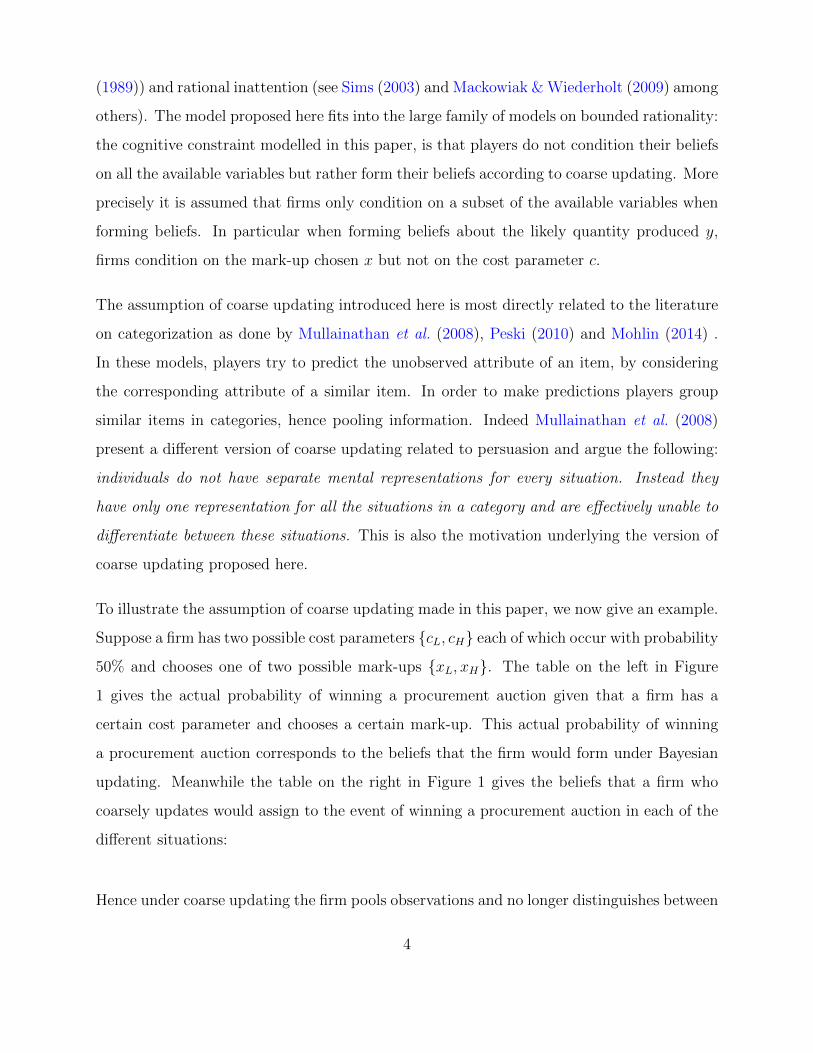
To illustrate the assumption of coarse updating made in this paper, we now give an example.
Suppose a firm has two possible cost parameters cL, cH each of which occur with probability
50% and chooses one of two possible mark-ups xL, xH. The table on the left in Figure
1 gives the actual probability of winning a procurement auction given that a firm has a
certain cost parameter and chooses a certain mark-up. This actual probability of winning
a procurement auction corresponds to the beliefs that the firm would form under Bayesian
updating. Meanwhile the table on the right in Figure 1 gives the beliefs that a firm who
coarsely updates would assign to the event of winning a procurement auction in each of the
different situations:
Hence under coarse updating the firm pools observations and no longer distinguishes between
4

xL
xH
cL cH
85 75
25 15
xL
xH
cL cH
80 80
20 20
=⇒Coarsening
Full Bayesian updating Coarse Bayesian updating
Figure 1: Coarsening of Beliefs
the two marginal costs cH and cL in determining its probability of winning when choosing
either mark-up. For instance the belief of winning the auction given a mark-up xL is used is
given to be 80% = (0.5× 85%) + (0.5× 75%).
Our primary motivation for considering coarse updating comes from the literature in psy-
chology on cue-competition. This literature examines how decision-makers predict a variable
that is stochastically related to multiple variables (or cues). One key finding is that a more
valid or more salient cue detracts from the learning of a less valid or less salient cue, and
that people do not achieve correct understanding of the correlation structure (Kruschke &
Johansen (1999) and Hirshleifer (2001)).
To show how this is relevant to our setting consider a decision-maker who is trying to predict
the output y, given that he observes both the mark-up chosen x and his marginal cost c.
A fully sophisticated Bayesian learner with prior f forms beliefs based on both variables as
follows:
Ω(y|x, c) =f(y, x, c)∑y f(y, x, c)
Now suppose that the mark-up variable x is highly correlated with output y, while the
marginal cost c is only weakly correlated with y. When a decision maker is cognitively-
constrained it seems likely that he will ignore the marginal cost variable c and just focus on
5

the more relevant mark-up variable x. In this case, he might use a coarse version of Bayesian
updating and form the following beliefs:
Ω(y|x) =∑c
f(y, x, c)∑y f(y, x, c)
Note that beliefs formed by coarse updating are insensitive to changes in marginal cost,
since firms who form beliefs using coarse updating disregard the cost parameter variable
when forming their beliefs. This feature of coarse updating leads to an equilibrium where
firms bid constant mark-ups because - unlike in the standard model - the beliefs of firms
do not depend on their marginal cost. Hence the assumption of coarse updating leads to a
model that is consistent with the fact that firms play constant mark-ups.
The motivation for choosing percentage mark-up to be the salient cue is that this variable
receives significant attention in the business literature: this makes it likely that it is a
variable firms monitor and is an important component of firms’ decision making. Moreover
considering coarse updating avoids problems associated with the standard model. As well
as capturing the fact that firms play according to constant mark-up strategies, a model with
coarse updating predicts that firms never set price equal to marginal cost. There is ample
evidence that this is indeed the case and that firms always choose prices strictly above their
marginal cost - see for example Baye & Morgan (2004). However an immediate implication
of the standard model is that the firm with highest marginal cost sets a price equal to its
marginal cost: moreover the prices all other firms set are derived from this initial condition.
Therefore all the results of the standard model are based on an initial condition, which is
not satisfied in reality. A significant advantage of the model proposed here is that it does
not suffer from such an objection.
Instead of modelling cognitive constraints directly, an alternative way to ensure players with
limited mental capacity choose simple strategies is to carefully design the model in such
a way that simple strategies are indeed optimal. This is done by Abreu & Brunnermeier
(2003) where investors are fully rational, but in equilibrium it is optimal for investors not
6

to condition on their private information when deciding how long to hold onto the asset.
Similarly in Klemperer (1999) bidders are fully rational, but in equilibrium it is optimal for
bidders not to condition on their valuation when deciding their mark-down. Eccles & Wegner
(2014) generalise these results giving conditions under which players have no incentive to
condition on their private information when choosing their action. In this paper we build on
this result and show that in certain cases where types are highly correlated, even sophisticated
firms who condition on all available variables have little incentive to deviate from a coarse
equilibrium.
A more direct way to ensure that firms bid according to mark-up pricing is to impose strategy
restrictions as proposed by Compte & Postlewaite (2013). Under strategy restrictions firms
submit linear bid functions before learning their cost: this means that after observing their
cost firms in general have an incentive to deviate. On the other hand under coarse updating
firms choose their bids after learning their costs: this ensures that firms have no incentive
to deviate and are behaving optimally at the interim stage. Therefore linear bid functions
arise indirectly due to the assumption of coarse updating, whereas they are imposed directly
when strategy restrictions are assumed. Finally both theories lead to different results: they
are not equivalent ways of looking at the same problem.
The model proposed in this paper can be used for the estimation of procurement auctions,
which has received considerable attention in the literature ( see for example Guerre et al.
(2000) and Athey & Haile (2002)). Existing estimation techniques for auctions with bidder
specific and hence asymmetric strategies - as proposed by Athey & Haile (2002) and Campo
et al. (2003) - require a very large number of observations. Our model could be used to
obtain player specific estimates for smaller data sets, leading to similar results when the
distribution of types approximately has the correlated structure discussed above. On the
other hand in settings where the analyst has external evidence that constant mark-up bidding
is being used, the estimation procedure proposed here could be used as an alternative to the
standard estimation procedure. We propose an estimation method for the model presented
in this paper.
7

The remainder of this paper is structured is follows. In section two we introduce the model
for the case of procurement auctions. The analysis of this model when the distribution of
costs is known follows in section three. Meanwhile section four investigates the case where
the distribution of prices is known and section five considers the estimation of the model.
Section six considers the case of more general case of Bertrand competition and finally section
seven concludes.
2 The model
We first consider the special case of a single unit private value procurement auction, where
the winner is paid his bid. A general model of Bertrand competition with a general demand
function is presented in section 6.
There is a set of firms denoted by I = 1, . . . , n. Each firm privately observes its marginal
cost ci ∈ R++. Having observed their costs, firms then simultaneously submit a price pi ∈
Pi = R+. We use c = (c1, . . . , cn) and p = (p1, . . . , pn) to refer to the vector of all firms’
costs and prices respectively. In a single unit procurement auction, only the firm setting
the lowest price produces, hence the quantity produced by firm i, given the vector of prices
submitted p is denoted by yi ∈ Yi = 0, 1 and is given as follows:
yi =
1 if pi < pj for all j 6= i
0 otherwise
We assume that in case of a tie, the contract is not awarded.
The profit earned by a firm is given by yi(pi − ci). Moreover it is assumed that marginal
costs are distributed according to a cumulative distribution function F : Rn++ 7→ [0, 1], where
Fi : (0,∞) 7→ [0, 1] for all i ∈ I.
Define Ci ⊆ (0,∞) to be the set of possible cost parameters for firm i. A pure strategy for
firm i is a mapping from possible cost parameters to prices, such that bi : Ci 7→ Pi. Applying
8

the bid function to the distribution of costs, creates a distribution of prices G : Rn+ 7→ [0, 1]
which can be written as follows:
G(p) =
∫Rn++
1bi(ci)≤pi for all i
f(c)dc
We complete the description of the model by defining the beliefs held by firms as follows:
Each firm i has a belief Ωi : Ci × Pi × Yi 7→ [0, 1]. The term Ωi(yi|pi, ci) captures the
probability firm i assigns to either winning (yi = 1) or losing (yi = 0) the auction given that
his marginal cost is ci and his price is pi. This belief structure is used to dovetail with the cue
competition theory used in psychology: here the player forms beliefs or predictions about yi
based on the variables (pi, ci). Coarse updating will involve dividing the space (pi, ci) into
categories and assigning one belief to each category.
2.1 Equilibrium
It is assumed that an equilibrium is formed by a set of strategy profiles (b1, ....bn) and a
set of beliefs (Ω1, ...,Ωn), one for each player. We will define two types of equilibrium: (i)
equilibrium under Bayesian updating and (ii) equilibrium under coarse updating, referred to
as coarse equilibrium. Equilibrium under Bayesian updating corresponds to the equilibrium
concept used in standard models where players form beliefs by conditioning on all available
information; meanwhile coarse equilibrium captures situations where players condition on
only some of the available information.
Under both equilibrium concepts firms choose their price in order to maximize profits. The
following optimality condition, states that no player believes that he has a profitable devia-
tion leading to a higher expected profit.2
2In the unlikely case that two or more prices maximize profit, it is assumed that the firm chooses thelowest of these prices:
9

Condition 1 (Optimality). For all ci
bi(ci) = min
arg max
pi
Ωi(1|pi, ci)ci − pi)
This condition has to be satisfied under any equilibrium definition.
Before turning to the second condition required for the definition of equilibrium we introduce
some additional notation. We use b−i to denote the set of bid functions (bj)j 6=i excluding the
bid function of player i and similarly write b−i(c−i) to denote the set of prices (bj(cj))j 6=i.
Moreover define φi(yi|pi, ci, b−i) to be the probability that firm i is awarded the contract
(yi = 1) or loses the auction (yi = 0) given (i) firm i submits a price pi, (ii) firm i has a
marginal cost of ci and (iii) opponents play according to strategies b−i. Hence:
φi(1|pi, ci, b−i) :=
∫Rn−1+
f(c−i|ci)1pi < bj(cj) for all j 6= i
dc−i (1)
φi(0|pi, ci, b−i) = 1− φi(1|pi, ci, b−i)
(2)
The second condition for equilibrium depends on the way in which beliefs are formed. We
therefore present two equilibrium definitions, one when firms form beliefs according to stan-
dard Bayesian updating, as well as one for coarse updating.
2.2 Bayesian updating
Under the first equilibrium concept it is required that firms update their beliefs according to
Bayes’ rule, conditioning on both their marginal cost ci and the price chosen pi. Therefore
the following condition must be satisfied:
Condition 2 (Bayesian updating). Suppose firms are playing according to strategies (b1, ..., bn)
and beliefs (Ω1, ...,Ωn) are formed according to Bayesian updating. Then beliefs are given as
10

follows:
Ωi(yi|pi, ci) = φi(yi|pi, ci, b−i)
Using these two conditions we can now define a Bayesian Nash equilibrium:
Definition 1. The set of strategy profiles (b1, ....bn) and the set of beliefs (Ω1, ...,Ωn) con-
stitute a Bayesian Nash equilibrium if they satisfy condition 1 optimality and condition 2
Bayesian updating.
As discussed above, standard models of price competition fail to explain certain findings, in
particular (i) the fact that firms often follow constant mark-up strategies and (ii) the fact
that firms never bid at marginal cost. In order to capture these findings in a model we
consider alternative assumptions on belief formation and in particular do not assume that
firms update their beliefs according to Bayesian updating.
2.3 Coarse updating
We now turn to the formation of beliefs under coarse updating. The term mark-up parameter
is used to refer to the term xi = pi/ci. Hence a mark-up parameter of 1 signifies that a firm
sets a price at marginal cost, whereas a mark-up parameter of 1.5 means that a firm sets a
price at a level equal to 150% of marginal cost. When firms form their beliefs according to
mark-up updating, we assume that they do not differentiate between two instances (xi, ci)
and (xi, c′i). In the terminology of the categorization literature, firms have one category
for each choice of mark-up xi ∈ X. Firms first partition the space P × Ci into categories
x ∈ X = R+, and then assign beliefs to each category x ∈ X.
The average of all instances within a category is computed to form the following condition
for mark-up updating:
Condition 3 (Coarse updating). Suppose firms are playing according to strategies (b1, ..., bn)
and beliefs (Ω1, ...,Ωn) are formed according to mark-up updating. Then beliefs are given as
follows:
Ωi(yi|xici, ci) =
∫ ∞0
φi
(yi|xici, ci, b−i
)fi(ci)dci
11
Since firms form their beliefs by taking an average over all marginal costs, beliefs do not
depend on marginal cost (assuming the mark-up xi is held constant). This is captured in
the following equation:
Ωi(yi|xici, ci) = Ωi(yi|xic′i, c′i) for all ci c′i (3)
In order to achieve an equilibrium under coarse updating, which we will refer to as coarse
equilibrium, it is required that firms form their beliefs conditioning only on the mark-up
chosen xi = pi/ci. and that the optimality condition is satisfied, with firms having no
incentives to deviate. This leads to the following definition:
Definition 2. The set of strategy profiles (b1, ....bn) and the set of beliefs (Ω1, ...,Ωn) consti-
tute an equilibrium under mark-up updating if and only if they satisfy condition 1 (optimality)
and condition 3 (mark-up updating).
Hence equilibria under coarse updating also preserve optimality from the firms’ point of
view: no player believes that he can profit from deviating. In this case only the mark-up
variable (x) is considered when forming beliefs.
3 Analysis with known distribution of costs
We now analyse the behaviour of firms under both Bayesian updating and coarse updating,
allowing to compare and contrast the outcomes resulting from the two ways of forming
beliefs.
3.1 Bayesian updating
The case where firms form their beliefs using Bayesian updating has been extensively studied
in the literature. Since firms are fully rational and form their beliefs by conditioning on all
variables the following lemma holds:
12

Lemma 3.1. Suppose beliefs (Ωi)i∈I and strategy profiles (bi)i∈I form an equilibrium under
Bayesian updating. Then for all ci and for all pi:
Ωi(1|pi; ci) =
∫Rn−1+
f−i(c−i|ci)1pi < bj(cj) for all j 6= i
dc−i
The maximization problem of firm i can now be written as follows:
maxpi
Ωi(1|pi; ci)(pi − ci)
(4)
Let ωi(1|pi; ci) denote the derivative of Ωi(1|pi; ci). This is the change in the firm’s belief
about how likely it is to win the contract when raising its price slightly. Differentiating
equation 4 with respect to pi and evaluating at pi = bi(ci) leads to:
ωi
(1|bi(ci); ci
)(bi(ci)− ci
)+ Ωi
(1|bi(ci); ci
)= 0 (5)
Re-arranging leads to the following proposition:
Proposition 3.2. Suppose beliefs (Ωi) and strategy profiles (bi)i∈I form an equilibrium under
Bayesian updating. Then for all i ∈ I and ci ∈ Ci the following condition is satisfied:
bi(ci) = ci +Ωi(1|bi(ci); ci)−ωi(1|bi(ci); ci)
Note that this is the standard equilibrium condition found in procurement auctions, written
in terms of a firm’s expectations. Closed form solutions can be obtained for different cost
distributions F , which determine the beliefs.
3.2 Coarse updating
Recall that in the case of coarse updating, firms only condition on the mark-up submitted
when predicting expected output. We now show that when players form beliefs according to
coarse updating, they bid according to constant mark-up strategies.
13

First note that in the case of mark-up updating firms do not condition on their marginal
cost when forming their beliefs about expected output. This leads to the following lemma:
Lemma 3.3. Suppose beliefs (Ωi)i∈I and strategy profiles (bi)i∈I form an equilibrium under
mark-up updating. Then for all ci and for all xi:
Ωi(1|xici; ci) =
∫Rn+f(c)1
xici < bj(cj) for all j 6= i
dc
Hence the belief of firm i about how likely it is to be awarded the contract, depends only on
the mark-up parameter xi:
Ωi(yi|xici; ci) = Ωi(yi|xic′i; c′i) for all ci, c′i (6)
In this case a firm ignores any information his marginal cost gives about relative competi-
tiveness, and assumes that his likelihood of being awarded the contract depends only on the
mark-up chosen. Crucially he associates low mark-ups with competitive bidding and high
mark-ups with uncompetitive bidding regardless of the absolute price level. This assump-
tion is particularly appropriate when firms experience mostly common shocks that affect the
marginal cost of all firms. We now make the following definition:
Definition 3. Suppose firms are playing according to constant mark-up strategies, where
bi(ci) = xici for all i. Then Qi(xi|x−i) is defined to be:
Qi(xi|x−i) =
∫Rn+f(c)1
xici < xjcj for all j 6= i
dc
Note that in the case of constant mark-up strategies the term Qi(xi, x−i) captures both (i) the
firm’s belief about the probability with which it wins the contract Qi(xi, x−i) = Ωi(1|xici; ci).
From now on - when constant mark-up strategies are being considered - the term Qi(xi, x−i)
will be referred to as the expected quantity produced.
We now define qi(xi|x−i) to be the derivative of Qi(xi|x−i) with respect to xi. Hence
Qi(xi|x−i) denotes the expected quantity produced, while qi(xi|x−i) denotes the rate of
14

change in expected quantity as the mark-up is increased and hence the likelihood with
which a firm goes from winning the auction to losing the auction by raising its price slightly.
Note that in a procurement auction −qi(xi|x−i) ≥ 0. Using this notation we now state the
following proposition:
Proposition 3.4. Suppose (b1, ...., bn) is an equilibrium under mark-up updating. Then
bidding strategies for all firms i ∈ I are linear and of the form bi(ci) = x∗i ci. Moreover the
following system of equations is satisfied:
x∗i = 1 +Qi(x
∗i |x∗−i)
−qi(x∗i |x∗−i)for all i ∈ I
This proposition states that any coarse equilibrium has a linear form. This stems from the
fact that firms disregard their cost parameter when thinking about their choice of mark-up:
rather than forming precise beliefs based both on the mark-up parameter xi and the cost
parameter ci they form beliefs based solely on the mark-up parameter xi. This removes any
incentive for firms to condition their mark-up on their marginal cost, and hence leads to
constant mark-up equilibria.
A partial intuition for this result can be given by considering the profit firm i expects to
earn given that (i) his marginal cost is ci, (ii) he submits a price bi(ci) = xici and (iii) other
firms play according to constant mark-ups bj(cj) = x∗jcj. We call this the subjective profit
function since it relates to the profits that firm i expects to receive, which may differ from
the profits a modeller would expect firm i to receive:
ΠSi (xi, x
∗−i|ci) = Qi(xi|x∗−i)(xi − 1)ci (7)
In equilibrium firm i must have no incentive to deviate. Hence differentiating this subjective
profit function with respect to the mark-up xi leads to the following first order condition:
δΠSi (xi, x
∗−i)
δxi=[qi(xi|x∗−i)(x∗i − 1) +Qi(xi|x∗−i)
]ci (8)
Setting the first order condition equal to 0 and rearranging leads to the following:
15

− qi(xi|x∗−i)(x∗i − 1) = Qi(xi|x∗−i) (9)
Here the left-hand side corresponds to the cost of raising the mark-up slightly, since the
expected quantity of goods sold will decrease. Meanwhile the right-hand side corresponds to
the benefit from raising the mark-up slightly, since goods will be sold at a greater margin.
In equilibrium all firms are behaving optimally and hence the benefit from raising the price
corresponds exactly to the cost of raising the price. Re-arranging the first order condition
this is the expression in proposition 3.4. This explains why any constant mark-up equilibrium
(x∗1, ..., x∗n) must satisfy the system of equations in proposition 3.4.
3.3 Existence
In the previous section we presented a property that any coarse equilibrium must satisfy. We
now introduce two conditions which ensure that such a constant mark-up equilibrium does in
fact exist when firms form beliefs according to coarse updating. One way to ensure existence
is to put conditions on the primitives of the model, namely the distribution functions (Fi)i∈I .
However in order for our conditions to be easily interpretable, we choose instead to place
conditions on the subjective profit functions (ΠSi )i∈I that describe the profits firms expect to
receive from playing certain constant mark-up strategies. These profit functions are defined
in the previous section in terms of the primitives. The first condition ensures that price cuts
from rivals never induce a firm to raise its prices:
Assumption 1. Suppose that for all ci:
ΠSi (xi, x−i|ci) ≥ ΠS
i (xi, x−i|ci) for all xi
ΠSi (xi, x−i|ci) ≥ ΠS
i (xi, x−i|ci) for all xi
then if element by element x−i ≥ x−i, then xi ≥ xi.
16

This condition says the following. Suppose playing a mark-up xi is an optimal mark-up
when opponents are playing mark-ups x−i. Now if opponents lower their mark-ups to some
x−i ≤ x−i, then any new optimal mark-up xi will be weakly below the previous mark-up
xi. In other words it is never optimal to increase the mark-up in response to opponents
decreasing their mark-up. When the mark up played by opponents is higher, player i’s
optimal mark-up is also weakly higher. This captures most real-life situations, where more
competitive bidding from one firm is typically met with more competitive bidding from
others. The second condition effectively puts a ceiling on the level that mark-ups can reach:
Assumption 2. There exists xi such that whenever xi ≥ xi and xi ≥ xj for all j then:
ΠSi (xi.x−i|ci) ≥ ΠS
i (xi, x−i|ci) whenever xi > xi
This condition says that for every firm i there exists a ceiling xi with the following property.
Whenever firm i is submitting a mark-up which is both (i) above the ceiling xi and (ii)
above the mark-up of every other player xj then firm i weakly prefers not to raise its mark-
up further. This condition captures the fact that when firms are bidding sufficiently high,
the benefits of undercutting and submitting a mark-up xi < xj outweigh the benefits of
continuing to bid a high mark-up. This captures most real-life situations, where excessively
high mark-ups give the firm choosing the highest mark-up an incentive to cut prices in order
to increase the probability of winning.
Proposition 3.5. Suppose assumption 1 and assumption 2 hold. Then there exists a coarse
equilibrium of the form bi(ci) = x∗i ci for all i ∈ I.
This proposition shows that existence of equilibrium can be guaranteed by adding two mild
assumptions which are often satisfied in applications.
3.4 Efficiency
In this section we investigate the efficiency of a procurement auction when players use coarse
updating. Given the existence conditions above hold, in the case of two symmetric firms we
17

can give a closed form solution for the mark-up that firms use:
Proposition 3.6. Consider two symmetric firms where F (c1, c2) = F (c2, c1). Suppose as-
sumptions 1 and 2 are satisfied. Then there exists a symmetric equilibrium where firms bid
bi(ci) = x∗ci where x∗ is given by:
x∗ =2∫ cccf(c, c)dc
2∫ cccf(c, c)dc− 1
Propositions 3.4 and 3.6 immediately imply that when two symmetric firms play according
to the symmetric equilibrium in a procurement auction, the auction is efficient. The firm
with the lowest cost submits the lowest bid, since in this equilibrium all firms multiply
their cost by the same constant mark-up. Therefore the firm with the lowest cost wins the
auction. Note however that in general the outcome of procurement auctions under mark-up
updating need not be efficient. In particular when firms’ costs are drawn from asymmetric
distributions, they may set different mark-ups. In this case if the firm with the lowest cost
is also setting a higher mark-up than some of its competitors, the firm’s bid may be higher
than that of it’s opponents. This leads to an inefficient outcome.
3.5 Correlated costs
We now investigate particular cases where costs are correlated. These cases of cost corre-
lation are important because a higher marginal cost for one firm is often associated with a
higher marginal cost for other firms. Indeed using independent types as a benchmark seems
inadequate in the case of procurement auctions, where costs tend to be highly positively cor-
related. This section shows that when the distribution structure of firms’ costs is correlated
in a certain way, there is little incentive for firms to deviate from a coarse equilibrium.
We restrict attention to case of a procurement auction with two firms, although results could
easily be generalised to cover n firms. The parameter θ represents some common component
that affects the cost of both firms, while zi and zj represent firm specific elements of the
cost. In particular the cost of player i is given to be ci = θ(1 + τzi). The parameter τ is a
18

measure of the degree of correlation of firms’ costs. When τ = 0 both firms have the same
cost and hence costs are perfectly correlated. Here we consider the case where τ → 0. It is
assumed that θ is drawn from some cumulative probability distribution G(θ) with derivative
g(θ). Furthermore the parameters zi and zj are independently drawn from some distributions
Hi(zi) and Hj(zj), with supports [zi, zi] and [zj, zj] respectively. It is further assumed that
z = minzi, zj > 0 and z = maxzi, zj <∞.
In order to make comparisons between coarse equilibrium and Bayesian equilibrium we intro-
duce the concept of ε-Bayesian equilibrium. Under an ε-Bayesian equilibrium firms cannot
increase their expected profits by more than a fraction ε by deviating to another strategy.
Definition 4. The strategy profile (bi, bj) is an ε-Bayesian equilibrium if for all ci and for
all pi
(bi(ci)− ci
)∫R+
1bi(ci) < bj(cj)
dcj ≥
1
1 + ε
(pi − ci
)∫R+
1pi < bj(cj)
dcj
For a fixed G(θ) as τ → 0 and costs become perfectly correlated, the equilibria reached by
coarse updating are also ε-Bayesian equilibria:
Proposition 3.7. Suppose there exists a K such that∣∣∣ θg′(θ)g(θ)
∣∣∣ < K for all θ ∈ [0,∞). Then
for all ε there exists a τ ∗(ε) such that whenever 0 < τ < τ ∗(ε), any coarse equilibrium is an
ε-Bayesian equilibrium.
Therefore as long as G is sufficiently smooth and τ is sufficiently small, any coarse equilibrium
is also an ε-Bayesian equilibrium. This result stems from the fact that when τ is small, firms
do not know whether their cost is relatively low or high compared to that of their opponents.
This makes it optimal for firms not to condition their mark-up on their marginal cost. The
next result focuses on a particular distribution of G in order to tackle the case where τ is
not necessarily small:
19

Proposition 3.8. Suppose
g(θ) =
δθδ
2θif θ ≤ 1
δθ−δ
2θif θ > 1
For all ε > 0 for all τ > 0 there exists a δ∗(ε, τ) such that whenever 0 < δ < δ∗(ε, τ), any
coarse equilibrium is an ε-Bayesian equilibrium.
This shows that whenever g(θ) ≈ 1θ, then any coarse equilibrium is approximately a Bayesian
equilibrium. This results stems from the fact that when θ is drawn from an uninformative
prior, firms do not know whether their realisation of the cost is likely to be relatively high
or low compared to that of the other firm.
This section shows that when firms’ costs are correlated in one of two particular ways, coarse
updating leads to equilibria that are approximately Bayesian equilibria. First when τ is small
and costs are highly correlated firms cannot deduce their position in the distribution from
their marginal cost, and coarse equilibria are ε-Bayesian equilibria. Secondly when g(θ) is
approximately distributed according to the uninformative prior, then similarly firms do not
receive information about how their marginal cost compares to that of the other firm. As
is shown in Eccles & Wegner (2014), in this case there exist Bayesian equilibria where firms
do not condition on their marginal cost. To summarise, coarse updating are ε-Bayesian
equilibria in those settings where firms’ costs provide them little rank information.
4 Analysis with known distribution of prices
In this section we show how the firms’ costs and the equilibrium mark-ups can be recovered
from the distribution of prices. We now assume that firms play according to a constant mark
up equilibrium bi(ci) = cix∗i as generated by the model and that the resulting distribution
of prices is given by G(p) Note that from differentiability of F , it follows that G(p) is
differentiable and hence we can use g(p) to denote the corresponding pdf. From now on we
20
restrict attention to procurement auctions, though similar results could be obtained whenever
the demand function is known.
The term Qi(x∗i |x∗−i) denotes the expected quantity firm i produces in equilibrium and -
given the demand function is known - can directly be calculated from the distribution of
prices:
Qi(xi|x−i) =
∫Rn+
1pi<pj for all j 6=i
g(p)dp (10)
Secondly the term Qi(x∗i (1+ε)|x∗−i) captures the expected quantity firm i would have received
had he increased his mark-up parameter by a proportion ε and hence set prices using the bid
function b(ci) = cix∗i (1+ε). This term can be calculated by inflating the price submitted by a
proportion ε and observing the new winner of the auction. Hence the term Qi(x∗i (1 + ε)|x∗−i)
can also be observed directly, and is given as follows:
Qi(x∗i (1 + ε)|x∗−i) =
∫Rn+
1pi(1+ε)<pj for all j 6=i
g(p)dp (11)
Finally by taking the limit as ε→ 0 the term −x∗i qi(x∗i |x∗−i) can be deduced:
− x∗i qi(x∗i |x∗−i) = limε→0
Qi(x∗i |x∗−i)−Qi(x
∗i (1 + ε)|x∗−i)
ε(12)
We now return to the original formula for calculating mark-ups:
x∗i = 1 +Qi(x
∗i |x∗−i)
−qi(x∗i |x∗−i)(13)
Although Qi(x∗i |x∗−i) is easy to calculate, it is difficult for the econometrician to recover the
term qi(x∗i |x∗−i) directly: the effects of slight variations in prices can be observed, but since
x∗ is not known, the econometrician cannot evaluate the effect of a slight change in the
mark-up. In order to deal with this problem, we re-arrange equation 13 to give:
x∗i =−x∗i qi(x∗i |x∗−i)
−x∗i qi(x∗i |x∗−i)−Qi(x∗i |x∗−i)(14)
21

As shown above both Qi(x∗i |x∗−i) and −x∗i qi(x∗i |x∗−i) can be calulated from the distribution of
prices. This means that the mark-up of each player can be calculated from the distribution
of prices. This result is summarised in the following proposition:
Proposition 4.1. Suppose firms are playing according to a coarse equilibrium and the distri-
bution of prices is given by G. Then there is a unique distribution of costs F that generates
this distribution of prices. Moreover in the case of a two player procurement auction, the
mark-up of each firm is given by:
x∗i =
∫∞0pig(pi, pi)dpi∫∞
0pig(pi, pi)dpi −
∫∞0
∫∞pig(pi, pj)dpjdpi
This proposition shows that the model is identified: every distribution G of outcomes deter-
mines a unique distribution F of primitives. Moreover when the distribution G of prices is
known then the mark-up parameters (x∗1, ..., x∗n) chosen by firms are uniquely determined.
4.1 Cost Dispersion
Theoretical models often struggle to explain the high variation of prices observed in reality,
as doing so typically requires some firms to set unreasonably high mark-ups and a large
dispersion of costs. A notable exception is Krasnokutskaya (2011) who significantly reduces
mark-ups required to create a price dispersion of a magnitude observed in practice, by
considering unobserved auction heterogeneity. We now take the distribution of prices G
is fixed and determine the corresponding distribution of costs under coarse updating and
under Bayesian updating respectively. We restrict attention to the case where players are
symmetric, although we allow for costs to be correlated.3
We say that a distribution F generates G under a coarse (Bayesian) equilibrium if there
exists a coarse (Bayesian) equilibrium (b1, b2) such that F (c1, c2) = G(b1(c1), b2(c2)). With
this terminology in mind, we now state the following proposition:
3We believe similar results would hold for the asymmetric case.
22
Proposition 4.2. Consider a two-player procurement auction with distribution of prices
G : [p, p]2 7→ [0, 1] where G(p1, p2) = G(p2, p1). Suppose the distribution F (1) : [c1.c1] 7→ [0, 1]
generates G under a coarse equilibrium and F (2) : [c2.c2] 7→ [0, 1] generates G under a
Bayesian equilibrium. Then:
1. [c1, c1] ⊂ [c2, c2]
if and only if
2. 2∫R+pig(pi, pi)dpi > pg(p, p) + 1
This proposition gives a necessary and sufficient condition for the cost distribution obtained
when considering coarse updating to be a strict subset of the cost distribution obtained when
considering Bayesian updating. This condition is satisfied for many distributions, such as
when prices are drawn independently from a uniform distribution on [a, b] (with 2a < b).
This shows that for a wide range of price distributions coarse updating leads to less cost
dispersion than Bayesian updating. This suggests that the standard model may predict too
much cost dispersion because it assumes firms are more sophisticated than they actually
are. The less cognitively demanding theory of coarse updating predicts less cost dispersion,
which is in line with the empirical evidence. This lends further credibility to the theory of
coarse updating.
5 Estimation with a finite sample of prices
Although the estimation method proposed does not apply exclusively to procurement auc-
tions, we assume throughout that the demand function (Di)i∈I is known by the econometri-
cian. In procurement auctions this is typically the case. Moreover estimation of procurement
auctions has been dealt with in a large number of papers under varying assumptions. For
example, Guerre et al. (2000) provide a non parametric estimation technique for the case of
independent costs, while Athey & Haile (2002) allow for asymmetries as well as common val-
ues. Moreover Campo et al. (2003) propose a structural estimation method for private value
23
auctions with affiliated values allowing for asymmetric firms and Krasnokutskaya (2011) con-
siders unobserved auction heterogeneity in procurement auctions. The estimation procedure
proposed in this paper provides a way to estimate the mark-ups chosen by asymmetric firms.
Since in this model estimating the bid function reduces to estimating a single parameter,
the mark-up, the number of observations required to estimate firm specific and possibly
asymmetric bid functions is significantly smaller than in models previously considered.
5.1 Estimation procedure
Let N be the total number of auctions observed. First define the demand function Di(pi, p−i)
as follows:4
Di(pi, p−i) =
1 if pi < pj for all j 6= i
0 otherwise
(15)
Now let pi,k denote the bid of firm i in round k and p−i,k denote the bids of the firms other
than i in round k. Define yi,k = Di(pi,k, p−i,k). Let b+i,k,ε = pi,k(1 + ε) and b−i,k,ε = pi,k(1− ε)
represent the bid function where all prices are ε higher and respectively ε lower than the
actual price observed. Finally let y+i,k,ε = Di(p−i,k,ε, p−i,k) and y−i,k,ε = Di(p
+i,k, p−i,k) be the
hypothetical quantities firm i would have produced had it always bid ε lower or ε higher.
First note that Qi(x∗i |x∗−i) denotes the expected quantity that firm i produces, assuming that
all firms play according to the strategy profile bi(ci) = cix∗i . Hence a consistent estimator Qi
for Qi(x∗i |x∗i ) can be given as follows:
Qi =
∑yi
∑Nk=1 1yi,k = yi
N(16)
Secondly define the estimator Ri,ε as follows:
Ri,ε =
∑yi
∑Nk=1 1y+i,k,ε − y
−i,k,ε = yi
2Nε(17)
4A similar estimation procedure could be carried out for other demand functions not corresponding toprocurement auctions.
24
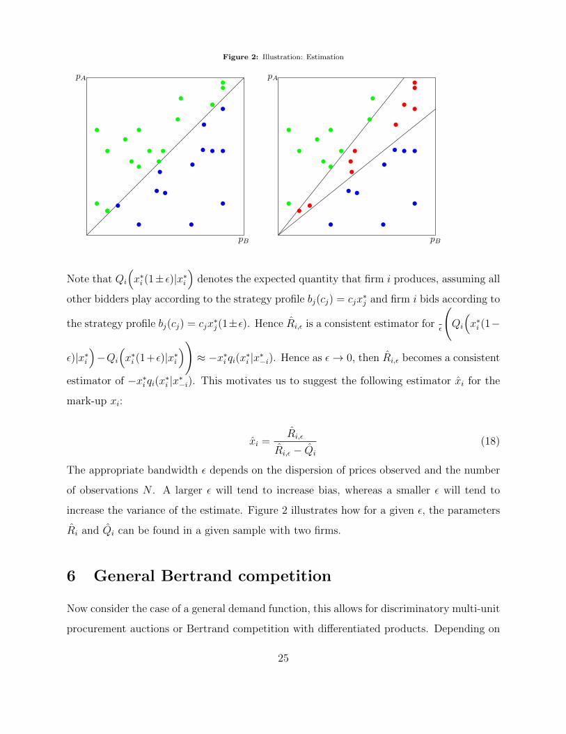
Figure 2: Illustration: Estimation
•
•
• •
•
•
•
•
••
•
•
•
•
•
•
• •
•
••
••
•
•
•
•
•
••
pB
pA
•
• •
•
•
••
••
•
•
•
•
•••
•
•
••
•
••
•
•
•
•
• •
pB
pA
Note that Qi
(x∗i (1± ε)|x∗i
)denotes the expected quantity that firm i produces, assuming all
other bidders play according to the strategy profile bj(cj) = cjx∗j and firm i bids according to
the strategy profile bj(cj) = cjx∗j(1±ε). Hence Ri,ε is a consistent estimator for
ε
(Qi
(x∗i (1−
ε)|x∗i)−Qi
(x∗i (1+ε)|x∗i
))≈ −x∗i qi(x∗i |x∗−i). Hence as ε→ 0, then Ri,ε becomes a consistent
estimator of −x∗i qi(x∗i |x∗−i). This motivates us to suggest the following estimator xi for the
mark-up xi:
xi =Ri,ε
Ri,ε − Qi
(18)
The appropriate bandwidth ε depends on the dispersion of prices observed and the number
of observations N . A larger ε will tend to increase bias, whereas a smaller ε will tend to
increase the variance of the estimate. Figure 2 illustrates how for a given ε, the parameters
Ri and Qi can be found in a given sample with two firms.
6 General Bertrand competition
Now consider the case of a general demand function, this allows for discriminatory multi-unit
procurement auctions or Bertrand competition with differentiated products. Depending on
25

the prices submitted, each firm faces demand yi = Di(pi, p−i) where yi ∈ 0, 1, 2, ..., K.
Again profits are given by πi(yi, pi, ci) = yi(pi − ci), now allowing for yi ∈ 1, . . . , k.
Similarly the definition of beliefs is modified to allow for different levels of production yi ∈
0, 1, 2, ..., K. Each firm i has a belief Ωi : Ci × Pi × Yi 7→ [0, 1]. The term Ωi(yi|pi, ci)
captures the probability firm i assigns to producing a quantity exactly equal to yi, given
that his marginal cost is ci and his price is pi. The optimality condition, taking expectations
across all possible levels of production becomes:
Condition 4 (General Optimality ). For all ci
bi(ci) = min
arg max
pi
Ki∑yi=0
Ωi(yi|pi, ci)πi(ci, pi, yi)
Furthermore, define φi(yi|pi, ci, b−i) to be the probability that firm i produces a quantity yi
given (i) firm i submits a price pi, (ii) firm i has a marginal cost of ci and (iii) opponents
play according to strategies b−i. Hence:
φi(yi|pi, ci, b−i) :=
∫Rn−1+
f(c−i|ci)1yi=Di
(pi,b−i(c−i)
)dc−i (19)
Given φ, the equilibrium condition for belief formation under Bayesian updating is the same
as in the special case of a single unit procurement auction, allowing for different levels of
production yi ∈ 1, . . . , k.
Condition 5 (Bayesian updating (General) ). Suppose firms are playing according to strate-
gies (b1, ..., bn) and beliefs (Ω1, ...,Ωn) are formed according to Bayesian updating. Then for
all i ∈ I, yi ∈ 1, . . . , K, pi ∈ Pi and ci ∈ Ci, beliefs are given as follows:
Ωi(yi|pi, ci) = φi(yi|pi, ci, b−i)
Similarly the condition for belief formation under coarse updating remains unchanged, except
for allowing different levels of yi.
26

Condition 6 (Coarse updating (General)). Suppose firms are playing according to strategies
(b1, ..., bn) and beliefs (Ω1, ...,Ωn) are formed according to mark-up updating. Then beliefs are
given as follows:
Ωi(yi|xici, ci) =
∫ ∞0
φi
(yi
∣∣∣xici, ci, b−i)fi(ci)dciNote that the definitions of equilibrium under Bayesian updating and under mark-up updat-
ing remain unchanged. Definitions 1 and 2 also apply in the case of Bertrand competition
with a general demand function.
In order to find equilibria in this case, define the quantity firm i expects to produce as
Ωi(pi; ci). This quantity is calculated by summing over the beliefs of firm i across all quan-
tities yi:
Definition 5 (Expected quantity).
Ωi(pi; ci) =K∑yi=0
yiΩi(yi|pi, ci)
The maximization problem of firm i can now be written as follows:
maxpi
Ωi(pi; ci)(pi − ci)
(20)
Taking first order conditions and setting them equal to zero leads to the following proposition:
Proposition 6.1. Suppose beliefs (Ωi) and strategy profiles (bi)i∈I form an equilibrium under
Bayesian updating. Then for all i ∈ I and ci ∈ Ci the following condition is satisfied:
bi(ci) = ci +Ω(bi(ci); ci)
−ωi(bi(ci); ci)
Now consider coarse updating with general Bertrand competition. We define Qi(xi|x−i) to
be the quantity firm i expects to sell, when it sets a mark-up xi and its competitors play
according to constant mark-up strategies x−i, when different levels of production are possible.
27

Definition 6. Suppose firms are playing according to constant mark-up strategies, where
bi(ci) = xici for all i. Then Qi(xi|x−i) is defined to be:
Qi(xi|x−i) =K∑yi=1
∫Rn+f(c)yi1
yi = Di
(pi, b−i(c−i)
)dc
In this case the firm’s maximization problem becomes:
maxxi
Qi(xi|x−i)(x∗i − 1)ci
(21)
Moreover the subjective profit that the firm expects to earn becomes:
ΠS(xi, x−i|ci) = Qi(xi|x−i)(x∗i − 1)ci (22)
We can now extend the result presented for procurement auctions above:
Proposition 6.2. Suppose assumption 1 and assumption 2 hold. Then there exists a coarse
equilibrium of the form bi(ci) = x∗i ci for all i ∈ I. Moreover (x∗1, ..., x∗n) satisfy the following
system of equations:
x∗i = 1 +Qi(x
∗i |x∗−i)
−qi(x∗i |x∗−i)for all i ∈ I
Therefore the equilibria under general Bertrand competition with a constant cost per unit,
have the same form as those in the special case of single unit procurement auctions.
7 Conclusion
In this paper we have used the psychological theory of cue competition to suggest a new model
for price competition that is consistent with a number of facts observed in practice. First
it is consistent with survey evidence, which suggests firms use mark-up pricing bidding and
bid a constant proportion of their marginal cost. Secondly it is consistent with experimental
evidence, which suggests firms never bid close to marginal cost. Thirdly the theory of coarse
updating tends to lead to less cost dispersion for a fixed price distribution than the standard
28

model. This is desirable, since one criticism of estimates based on the standard model is
that cost dispersion seems too high. Despite the large number of experiments conducted on
price competition and the survey and anecdotal evidence for mark-up pricing, - as far as we
are aware- there are no experiments that directly test for the use of mark-up pricing. Such
experiments may shed light on the importance of mark-up updating and provide additional
insight into how players choose bidding strategies.
A further advantage of the model proposed here is that preliminary simulations have shown
that it is easier to estimate than the standard model. This means that it can be estimated
with less data, and hence can be applied in a wider range of situations. In particular, a
procurement auction with more than two (asymmetric) firms is relatively easy to estimate
using the procedure outlined above, while this is difficult to estimate using the standard
model as discussed in Campo & Vuong (2003). Quantifying this advantage (ie how much
less data is needed), running further simulations and developing an application are all areas
for future work.
A final advantage of the model proposed here is that when costs are highly correlated beliefs
under coarse updating closely resemble beliefs under Bayesian updating. This means that
firms have little incentive to deviate from a coarse equilibrium. This case is particularly
relevant, because firms costs are often highly correlated.
There are at two distinct ways to extend the model of coarse updating proposed here. The
first extension is to consider a wider range of utility functions and not just to model Bertrand
competition. We believe this is a promising area for future research, since it allows to model
cognitively constrained agents in a tractable way.
The second extension involves considering different ways of categorising information. By
assuming that firms focus on the mark-up variable we implicitly define a mapping from
φ : Ci × Pi 7→ Xi: more precisely choosing φ(ci, pi) = pi/ci determines which categories are
evaluated together. Choosing different ways of categorising the information would lead to
different results. One obvious choice would be for firms to focus on the price variable and
29

choose φ(ci, pi) = pi. The reason this paper focuses on the mark-up variable is that (i) it is
widely discussed in the business literature and (ii) beliefs are almost correct when costs are
highly correlated. However investigating other ways of categorising information may also be
more relevant in other situations.
30

8 Appendix
8.1 Proof of proposition 3.4
Consider a mark-up equilibrium bi(ci). From the optimality condition, it follows that:
bi(ci)
ci= min
arg max
N∑yi=1
yiΩi(yi|xici, ci)(xi − 1)
Since Ωi(yi|xici, ci) = Ωi(yi|xi), the right hand side does not depend on ci. Hence the left hand
side does not depend on ci either. Therefore for some x∗i , it follows that bi(ci)ci
= x∗i and hence
bi(ci) = x∗i ci. It follows that all mark-up equilibria are in linear strategies.
8.2 Proof of proposition 3.5
Consider expected profits, namely Πi(xi, x−i|ci) = ci(xi−1)Qi(xi|x−i). Define BRi(x−i) as follows:
BRi(x−i) = min
arg maxxi∈[1,∞)
(xi − 1)Qi(xi|x−i)
Now define a sequence inductively as follows. First define x
(0)i = 1. Secondly define xk−i =(
x(k+1)1 , ...x
(k+1)i−1 , x
(k)i+1, ..., x
(k)n
)and finally define x
(k+1)i = BRi(x
(k)i ). Define also that x = maxxi.
We argue that (i) x(k+1)i ∈ [1, x], (ii) x
(k)i is weakly increasing, (iii) x
(k)i → x∗i and (iv) x∗ =
(x∗1, ..., x∗n) is an equilibrium.
In order to prove (i) BRi(x−i) ≥ 1 from the definition of BRi(x−i). Moreover suppose xj ≤ x
for all j 6= i. Then by assumption 2 BRi(x−i) ≤ x, since for any xi > x ≥ xi it follows that
Πi(xi, x−i|ci) ≤ Πi(x, x−i|ci).
In order to prove (ii) note from above that x(k)i ≥ 1. The result then follows by induction using
assumption 1: if x′−i ≥ x−i, then BRi(x′−i) ≥ BRi(x−i)
Moreover in order to prove (iii) note that x(k)i is a weakly increasing sequence which is bounded
above. Hence it converges to x∗i .
Finally to prove (iv) note that (xi − 1)Qi(xi|x−i) is continuous. Hence:
31

(x(k)i − 1)Qi(x
(k)i |x
(k)−i ) ≥ (xi − 1)Qi(x
(k)i |x
(k)−i )
Taking the limit as k →∞ yields:
(x∗i − 1)Qi(x∗i |x∗−i) ≥ (xi − 1)Qi(x
∗i |x∗−i)
Moreover by assumption 1 whenever xi < x∗i :
(x∗i − 1)Qi(x∗i |x∗−i) > (xi − 1)Qi(x
∗i |x∗−i)
Hence x∗i = min
arg maxxi
(xi − 1)Qi(xi|x∗−i)
and this proves the result.
8.3 Proof of proposition 3.6
From proposition 4.1, it follows that:
x∗i =
∫∞0 pig(pi, pi)dpi∫∞
0 pig(pi, pi)dpi −∫∞0
∫∞pig(pi, pj)dpjdpi
By symmetry x∗i = x∗j = x∗. Using the definition of G(pi, pj) and symmetry, it follows that
g(pi, pj) = 1x2f(pi/x, pj/x). Hence:
x∗ =
∫∞0 pif(pi/x, pi/x)dpi∫∞
0 pif(pi/x, pi/x)dpi −∫∞0
∫∞pif(pi/x, pj/x)dpjdpi
By symmetry∫∞0
∫∞pif(pi/x, pj/x)dpjdpi = 1/2. Substituting ci = pi/x leads to:
x∗ =2∫∞0 cif(ci, ci)dci
2∫∞0 cif(ci, ci)dci − 1
This proves the result.
8.4 Proof of proposition 3.7
It is enough to show that the beliefs formed using coarse updating are arbitrarily close to those
formed using Bayesian updating, given players are playing according to linear strategies bi(ci) =
x∗i ci. This will ensure that beliefs formed by Bayesian updating are very close to those formed
32

through coarse updating and ensures that players have no incentive to deviate from a coarse equi-
librium. If Ωi(y|xi) are the beliefs formed through coarse updating when the opponent plays a
strategy bi(ci) = xjci, then:
minci∈Ci
φi(1|xi, xj , ci)
≤ Ω(y|xi) ≤ max
ci∈Ci
φi(1|xi, xj , ci)
Hence it is enough to show that for all ci and c′i and all strategies xi and xj for any ε > 0 there
exist parameters δ or τ such that:
φi(1|xi, xj , ci)− φi(1|xi, xj , c′i) ≤ ε
Using the fact that F (cj |θ) = H(cj/θ) and f(cj |θ) = 1θh(cj/θ):
φi(1|xi, xj , ci) =
∫R+
g(θ|ci)f(cj |θ)1xici ≤ xjcjdcjdθ
=
[∫R+
g(θ)f(ci|θ)dθ
]−1 ∫R+
f(ci|θ)g(θ)F(xicixj
∣∣∣θ)dcjdθ=
[∫R+
g(θ)
θh(ci/θ)dθ
]−1 ∫R+
g(θ)
θh(ci/θ)H
(xicixjθ
)dθ
Substituting t = ciθ and s = ci
θwe reach:
φi(1|xi, xj , ci) =
[∫R+
g(ci/s)
sh(s)ds
]−1 ∫R+
g(ci/t)
th(t)H
(xitxj
)dt
Let m = (1 + τz) and m = (1 + τz). Recall that (1 + τz)θ ≤ ci ≤ (1 + τz)θ and hence m =
(1 + τz) ≤ t ≤ (1 + τz) = m Hence the integral can be rewritten as follows:
33

φi(1|xi, xj , ci) =
[∫ m
m
g(ci/s)
sh(s)ds
]−1 ∫ m
m
g(ci/t)
th(t)H
(xitxj
)dt
8.5 Proof of proposition 3.8
For the first case suppose g(θ) has the specific form given in the text. Then g(ci/t)t = δ
2ci
(cit
)δwhen
ci < t and g(ci/t)t = δ
2ci
(cit
)−δwhen ci > t. We now claim that for any t ≤ s and for any ci:
(t/s)δ≤ g(ci/t)
t
/g(ci/s)
s≤(s/t)δ
There are three cases. First assume t ≤ ci and s ≤ ci. Then g(ci/t)t = δ
2ci
(cit
)−δand g(ci/s)
s =
δ2ci
(cis
)−δ. Dividing g(ci/t)
δt
/g(ci/s)δs leads to the inequality.
Secondly assume t ≥ ci and s ≥ ci. Then g(ci/t)t = δ
2ci
(cit
)δand g(ci/s)
s = δ2ci
(cis
)δ. Again dividing
g(ci/t)δt
/g(ci/s)δs leads to the inequality.
Third assume t ≤ ci ≤ s. Then using case (i) it follows that:
(t/ci
)δ≤ g(ci/t)
t
/g(ci/ci)
ci≤(ci
/t)δ
Similarly using case (ii) it follows that:
(ci
/s)δ≤ g(ci/ci)
ci
/g(ci/s)
s≤(s/ci
)δMultiplying these inequalities together we reach case (iii):
(t/s)δ≤ g(ci/t)
t
/g(ci/s)
s≤(s/t)δ
Recall that t and s in [m,m] and hence for any ci:
(m/m)δ≤ g(ci/t)
t
/g(ci/s)
s≤(m/m)δ
34

As δ → 0 this term goes to 1. Hence as δ → 0:
φi(1|xi, xj , ci) =
[∫ m
m
g(ci/s)
sh(s)ds
]−1 ∫ m
m
g(ci/t)
th(t)H
(xitxj
)dt
=
∫mm h(t)H
(xitxj
)dt
∫mm
[g(ci/s)s
/g(ci/t)t
]h(s)ds
For δ ≤ ε4 log(m)−log(m) = δ∗(ε) the term in square brackets is between (1− ε/2) and (1 + ε/2) for all
ci. Hence whenever δ < δ∗(ε), then φi(1|xi, xj , ci)−φi(1|xi, xj , c′i) ≤ ε for all ci and c′i. This proves
the result.
8.5.1 Case with small τ
Again we aim to prove that g(ci/t)t
/g(ci/s)s is close to 1 in the interval [m,m] whenever τ is sufficiently
small. First note that as τ → 0, then m → 1 and m → 1. Hence it is sufficient to prove that for
any δ ≤ δ∗(ε):
1− ε ≤g(ci/(t+ δ)
)t+ δ
/g(ci/t)
t≤ 1 + ε
To prove define φ(t) = g(ci/t)t . It is enough to show that φ′(t)/φ(t) is uniformly bounded. Computing
this expression leads to:
∣∣∣φ′(t)φ(t)
∣∣∣ =∣∣∣cig′(ci/t)t− g(ci/t)
t2
/g(ci/t)
t
∣∣∣=
1
t
∣∣∣ci/tg′(ci/t)g(ci/t)
− 1∣∣∣
=1
t
∣∣∣θg′(θ)tg(θ)
− 1∣∣∣
Since t ∈ [m,m] it follows that∣∣∣φ′(t)φ(t)
∣∣∣ < K whenever θg′(θ)g(θ) is uniformly bounded. From here the
result follows.
35
8.6 Proof of proposition 4.1
First note that:
Qi(x∗i |x∗j ) =
∫R2+
f(ci, cj)1x∗i ci < x∗jcjdcidcj (23)
If firms are playing according to coarse equilibrium strategies then ci = pi/x∗i . Note - from the
definition of G(pi, pj) - that f(ci, cj) = x∗ix∗jg(cix
∗i , cjx
∗j ). Substituting (pi, pj) for (ci, cj) leads to:
Qi(x∗i |x∗j ) =
∫Rn−1+
g(pi, pj)1pi < pjdpidpj
=
∫ ∞0
∫ ∞pi
g(pi, pj)dpjdpi (24)
(25)
Secondly note that:
−x∗i qi(x∗i |x∗−i) = xi
∫ ∞0
cixjf(ci,cixixj
)dci
=
∫ ∞0
cixixjf(cixj , cixi
)dci
=
∫ ∞0
cix2ix
2jg(cixjxi, cixixj
)dci (26)
(27)
Substituting pi for cixixj leads to:
− x∗i qi(x∗i |x∗−i) =
∫ ∞0
pig(pi, pi)dpi (28)
Finally recall that by equation 14:
x∗i =−x∗i qi(x∗i |x∗−i)
−x∗i qi(x∗i |x∗−i)−Qi(x∗i |x∗−i)(29)
Applying equations 24 and 28 proves the result.
36

8.7 Proof of proposition 4.2
By proposition 3.2 under Bayesian updating:
b(c) = c+Ωi(1|b(c); c)−ωi(1|b(c); c)
Note that b(c) = p and Ωi(1|p; c) = 1. Moreover the chance of winning when submitting a bid p
with marginal cost c is Ωi(1|p, c) = G(p|b(c)
). Differentiating with respect to p and evaluating at
p = p and c = c leads to ωi(1|p, c) = g(p|p). Hence:
c2 = p− 1
g(p|p)
See Athey & Haile (2007) for a similar formula for standard auctions. On the other hand under
coarse updating:
c1 = p[ ∫∞
0 pig(pi, pi)dpi∫∞0 pig(pi, pi)dpi −
∫∞0
∫∞pig(pi, pj)dpjdpi
]Simple algebraic manipulation shows that c2 < c1 if and only if
2
∫R+
pig(pi, pi)dpi > pg(p, p) + 1
This proves the proposition.
37
References
Abreu, D., & Brunnermeier, M. 2003. Bubbles and Crashes. Econometrica, 71, 173204.
An, Y., Hu, Y., & Shum, M. 2010. Estimating first-price auctions with an unknown number of
bidders: A misclassification approach. Journal of Econometrics, 157, 328–341.
Arthur, W. B. 1994. Inductive Reasoning and Bounded Rationality. American Economic Review,
84, 406–411.
Athey, S., & Haile, P. 2002. Identification of Standard Auction Models. Econometrica, 70, 21072140.
Athey, S., & Haile, P. 2007. Handbook of Econometrics. Vol. 6 A. Elsevier. Chap. Nonparametric
Approaches to auctions, pages 3847–3965.
Aumann, R., & Sorin, S. 1989. Cooperation and Bounded Recall. Games and Economic Behaviour,
1, 5–39.
Baye, M., & Morgan, J. 2004. Price dispersion in the lab and on the Internet: Theory and evidence.
Rand Journal of Economics, 35, 449–466.
Campo, S., Perrigne I., & Vuong, Q. 2003. Asymmetry in first-price auctions with affiliated private
values. Journal of Applied Econometrics, 18, 179–207.
Campo, S., Perrigne, I., & Vuong, Q. 2003. Asymmetry in first-price auctions with affiliated private
values. journal of Applied Econometrics, 18, 179–207.
Compte, O., & Postlewaite, A. 2013. Simple Auctions. PIER Working Paper 13-017.
Crawford, V., & Irriberri, N. 2007. Level- k auctions: Can a nonequilibrioum model of strategic
thinking explain the winner’s curse and overbidding in private- value auctions? Econometrica,
75, 1721–1770.
Eccles, P., & Wegner, N. 2014. Scalable Games. Working paper.
Fabiani, S., Gatulli, A., Veronese, G., & Sabbatini, R. 2010. Price adjustment in Italy: evidence
from micro producer and consumer prices. Managerial and Decision Economics, 31, 93104.
38

Greenslade, J., & Parker, M. 2010. New insights into price-setting behaviour in the United Kingdom.
Bank of England Working Paper.
Greenslade, J., & Parker, M. 2012. New Insights into Price- Setting Behaviour in the UK: Intro-
duction and Survey Results. Economic Journal, 122, F1–F15.
Guerre, E., I., Perrigne, & Vuong, Q. 2000. Optimal Nonparametric Estimation of First-Price
Auctions. Econometrica, 68, 525–574.
Hirshleifer, D. 2001. Investor Psychology and Asset Pricing. Journal of Finance, 56, 1533–1597.
Kahnemann, D., & Tversky, A. 1981. The Framing of Decisions and the Psychology of Choice.
Science, 211, 453–458.
Klemperer, P. 1999. Auction Theory: A guide to the literature. Journal of Economic Surveys, 13,
227–286.
Krasnokutskaya, E. 2011. Identification and Estimation of Auction Models with Unobserved Het-
erogeneity. Review of Economic Studies, 28.
Kruschke, J. M., & Johansen, M.K. 1999. A model of probabilitsic capacity learning. Journal
Journal of Experimental Psychology, Learning and Cognition, 25.
Mackowiak, B., & Wiederholt, M. 2009. Optimal Sticky Prices under Rational Inattention. Amer-
ican Economic Review, 99, 769–803.
Mohlin, E. 2014. Optimal Categorization. Journal of Economic Theory, 152, 356–381.
Mullainathan, S., Schwartzstein, J., & Shleifer, A. 2008. Coarse Thinking and Persuasion. Quarterly
Journal of Economics, 123, 577–619.
Nagel, R. 1995. Unraveling in Guessing Games. American Economic Review, 85, 1313–1326.
Peski, M. 2010. Prior symmetry, similarity based reasoning, and endogeneous categorization. Jour-
nal of Economic Theory, 126, 111–140.
Rothkopf, M. 1980. On Multiplicative Bidding Strategies. Operations Research, 28, 570–575.
39

Rubinstein, A. 1998. Modeling Bounded Rationality. Cambridge, Mass : MIT Press.
Sims, C. 2003. Implications of rational inattention. Journal of Monetary Economics, 50, 665–690.
Sorensen, A. T. 2000. Equilibrium Price Dispersion in Retail Markets for Prescription Drugs.
Journal of Political Economy, 108, 833–850.
Stahl, H. 2005. Price setting in German manufacturing: new evidence from new survey data.
Deutsche Bundesbank: Working Paper.
40