CONTRACTIONARY DEVALUATION AND CREDIT

CRUNCH:

ANALYSING ARGENTINA

Co-authored by

Marcus Miller, Javier Garcia Fronti & Lei Zhang

CSGR Working Paper Series No 190/06

January 2006

Contractionary devaluation and credit crunch:

analysing Argentina ∗

Marcus Miller †, Javier Garcıa Fronti ‡and Lei Zhang §

October 2005

Abstract

Sharp economic contraction often follows currency devaluation in emerging markets –

due mainly to liability dollarisation. Such adverse balance sheet effects play a key role in

the well-known model of Aghion et al (2000), by reducing investment and future supply.

We show how the prompt contraction of output can accounted for by incorporating

demand failure – due to a slow export response and a credit crunch. The resulting eclectic

framework is used to study the collapse of the Argentine economy when Convertibility

ended in 2002; and to see why efforts to imitate President Roosevelt by ‘pesifying’ the

economy proved counter-productive.

Key words: Contractionary devaluation, Keynesian recession, Argentine economic crisis,

asymmetric pesification

JEL Classification: E12, E51, F34, G18

Contact author: marcus.miller@warwick.ac.uk

∗For comments and suggestions, we thank Santiago Acosta-Ormaechea, Philippe Aghion, Lisandro

Barry, Mario Blejer, Luis Cespedes, Guillermo Escude, Matthew Fisher, Daniel Heymann, Daniel Laskar,

Andrew Powell and Klaus Scdhmidt-Hebbel; but responsibility for views expressed is our own. The first

two authors are grateful to the ESRC for financial support supplied to the research project RES-051-27-

0125 “Debt and Development” and Lei Zhang for support from RES-156-25-0032. For research assistance,

we thank Elba Roo, funded in part by the CSGR.†University of Warwick and CEPR‡University of Warwick§University of Warwick

1

Non-technical Summary

Introduction

For emerging market economies, the initial impact of sharp devaluations is often con-

tractionary; and the most likely causal mechanism is currency mismatch in corporate

balance sheets (Frankel, 2004). Economies which are relatively closed but have substan-

tial borrowing denominated in dollars are particularly vulnerable to a sudden stop in

capital flows: dollar loans to the nontraded sector will be mismatched and the exchange

rate adjustment needed to service dollar debts will be large. Moreover, the vulnerability

can itself trigger sudden stops in capital flows, as pointed out by IADB in its 2005 Report

on Economic and Social Progress in Latin America.

Balance sheet effects hit non-financial companies directly; but banks can also act as a

potent transmission mechanism if they suffer from adverse balance sheet effects, for the

knock-on effects of the credit crunch can spread widely throughout the economy. This is

especially true in Latin America, where banks play a central role in corporate financing

(IADB Report, 2005, Introduction).

Recent events in Argentina have provided stark evidence of these risks and vulnera-

bilities. The economy was relatively closed, there was widespread currency miss-match

(about two thirds of corporate borrowing in dollars) and the currency was tied to a dol-

lar that rose strongly against key markets for Argentine exports. The ’convertibility’

regime, where the peso was fixed at parity with the US dollar, ended with a ’twin crisis’,

involving a tripling in the price of a dollar and a protracted closure of the entire banking

system, and an economic contraction so severe that it is referred to locally as “Nuestra

gran depresion”.

Even before the convertibility regime ended, the economy had been badly weakened.

A decade of pegging to a strong dollar had squeezed profits and ended growth; and the

government itself, with large dollar debts secured on a narrow tax base of largely domestic

producers, was a major source of currency mismatch. The failure to banish the spectre of

fiscal insolvency had eroded market confidence, raising sovereign spreads and weakening

investment; and the vulnerability of both government and banks led to draining capital

flight and deposit withdrawals.

2

When the peg finally collapsed, President Duhalde’s bold attempt to imitate Franklin

Roosevelt by pesifying dollar loan contracts, while simultaneously protecting dollar de-

positors, had the effect of destroying bank net worth as government promises to recapi-

talise lacked credibility. So the banking system closed down and the economy was thrown

into a depression.

Gerchunoff and Llach (2003) provide a graphic history of these events and a balanced

account of conflicting interpretations of the crisis is provided by Sgard (2004). The aim

of this paper is not, however, to debate why convertibility ended; it is rather see how, i.e.

to study the process of collapse and the proximate events that threw the country into

depression when the end came.

Using an explicit model

A dynamic analysis of balance sheet effects is included within the comprehensive two-

sector New Keynesian framework developed by Escude (2004), where exports are sold in

euros while debts are contracted in dollars. With sticky wages and service prices, dollar

appreciation causes unemployment and leads to a sudden stop in capital flows, followed

by devaluation and default. This inter-temporally optimising two-sector approach has

its attractions, but the continuous-time dynamic system is complex even without taking

account of the investment demand and their capacity effects.

Aghion, Bacchetta and Banerjee (2000) (hereafter ABB) provide a framework which

offers a neat characterisation of output and exchange rate determination in a small open

economy producing a traded good. One-period of price stickiness for the traded good is

enough to yield adverse balance sheet effects where a fall in the exchange rate induces a

supply-side contraction as investment is cut back, reducing productive potential in the

next period. There is goods market clearing and international asset arbitrage; but the

multiplicity of equilibria opens up the possibility of sudden shifts in the exchange rate

(an effect analogous to that of a Sudden Stop).

While the authors have subsequently gone on to include more detail on the role of

banks, they explicitly assume that “...banks have enough assets not to fall into insolvency

in case a currency crisis occurs.” (Aghion, Bacchetta and Banerjee 2004, p15). That this

is not appropriate for Argentina in 2002, we show by calculating the adverse effect of

3

default, devaluation and asymmetric pesification on banks’ balance sheets. It is suggested

that an interesting extension would be to incorporate bank currency exposure, where

currency depreciation can results in disruption of lending so that “... the credit multiplier

µ may be reduced ...” (Aghion, Bacchetta and Banerjee, 2004, p28). In this paper we

use the basic model of ABB, modified to allow for changes in the credit multiplier.

Another modification is to allow for a Keynesian demand-side recession. In the ABB

framework output is essentially supply determined: it is a small open economy model

where net exports always bring demand into line with supply. So a fall in investment, for

example, leaves current period output unchanged but reduces output in the next period.

But when investment collapsed in Argentina after devaluation and default in 2001/02,

output also fell sharply. Allowing for the demand-determination of output in the period

of collapse provides a richer framework for studying open economy crises in general — a

blend of the demand-side approach of Krugman (1999), Cespedes et al (2003,2004) and

the dynamic supply-side account of ABB. It also allows one to capture more realistically

what happened in Argentina. We show, for example, that, when it causes a demand side

recession, tight monetary policy is less likely to strengthen the currency.1

This eclectic approach is used to show first how pesification can, in principle, mitigate

adverse balance sheet effects; but how, mishandled, it can plunge the economy into chaos.

For when debt relief for corporations is achieved by making banks bankrupt, the outcome

can well be counter-productive, as the collapse of the banking system leads to a reduction

in the credit multiplier, less investment and less output.

Unfortunately, the prompt action taken by the Duhalde government to recapitalise

the banking system lacked credibility, and led to paralysis of the banking system, leaving

the country without credit for one year and a half. How could this outcome have been

avoided? One possible strategy was asymmetric pesification at a rate of 1.2. Under this

policy, depositors would be given some help and so too would producers: and the hits on

bank net worth would be smaller.But whether this was politically feasible is debatable.

The policy approach recommended by the IADB, on the other hand, would imply a

1Technically, if output in crisis period is demand-determined, an increase in the interest rate will lead

to a currency depreciation relative to that predicted by the ABB model.

4

more selective debtor bail-out; and a greater political commitment by the government

to meeting the costs of recapitalisation. The IADB Report of 2005 cites with approval

the actions taken later by Uruguay when it faced a similar crisis. Before considering

other policy alternatives, we contrast pesification in Argentina with Roosevelt’s earlier

initiative.

Comparing Argentine “pesification” with Roosevelt’s cancelation of the Gold

Clause

When the US was on the gold standard, long-term loan contracts were typically

indexed to the price of gold. In 1933, however, Congress passed a Resolution nullifying the

gold clauses in private and public debt. This abrogation was “ a key part of Roosevelt’s

‘first hundred days’, providing the foundation for much of the New Deal policies directed

at reflating the economy including departure of the US from the gold standard”, Kroszner

(2003, p.1). The validity of the Resolution was challenged in court when the US left the

gold standard a year later and the dollar price of gold rose by almost 70%. The Supreme

Court upheld the Resolution, however, mainly on the grounds that the plaintiffs had not

been harmed: in the case of one defendant, for example, it was argued that he did not

“ show in relation to buying power he has sustained any loss whatever” . On the day

the verdict was announced, corporate bonds whose gold clause was abrogated rose in

price – evidence, it appears, that cancelation promised a better return than enforcement,

Kroszner (2003, p.22).

This historical precedent led some observers to recommend devaluation-with-pesification

as an appropriate policy option for Argentinain 2001; and ?conomists in the IMF Research

Department also backed devaluation-with-default as a better option than borrowing more

to defend peso parity with the dollar. When the Convertibility regime ended in January

2002, President Duhalde of Argentina did in fact ‘pesify’ debt contracts, and Roosevelt

was explicitly cited as a precedent. Our application of the model is design to show why

the process of pesification, rather than helping to ameliorate the crisis as in the US, may

have played a key role in its propagation. This prompts the immediate question: what

was so different between these two cases? Kroszner (2003, p.4 and p.28) indicates two

factors: first unlike the US, the Argentine government engaged in ‘asymmetric’ pesifica-

tion; and second that Argentina may have suffered more from the lack of respect for the

5

rule of law involved in such across-the-board abrogation of contracts. These issues are

considered in some detail in the paper.

Policy alternatives

With time, the economy is on a recovery path. The government is paying compen-

sation to the banks; sovereign debt has been restructured; and sovereign spreads have

fallen below 5% in the summer 2005. But the fact that “ the economic collapse that

accompanied Argentina’s eventual default and devaluation was much deeper than neces-

sary to bring Argentina’s external accounts into some semblance of balance ... suggests

it is at least conceptually possible that an alternative policy path might have produced a

smaller fall in output.” (Roubini & Setser 2004, p.355). What alternative policies might

have helped?

A government itself facing a solvency crisis will inevitably face great difficulty in

restoring bank solvency: one must surely look for action that could been taken earlier

to forestall or minimise crisis. Note that Roosevelt took pre-emptive action nine months

before devaluing, by canceling the gold clause and imposing capital controls to conserve

US gold reserves. But in Argentina there were no capital controls until December 2001.

The capital account was left open — with capital flight estimated at $23 bn in 2000-1,

Bonelli (2004, p.216). So, despite IMF loans in early and mid-2001, official reserves ran

down sharply, falling by $20 billion between October 2000 - when the political crisis

began with the resignation of Vice President Alvarez - until the end of 2001, Bonelli

(2004, p.215).

It is widely agreed that Argentina should have devalued earlier, but the then govern-

ment was desperate that the peg should not fail. In these circumstances it should have

been warned of the need to limit capital outflows — but this advice would have been

inconsistent with the IMF’s commitment to financial liberalisation. The result was an

open capital account, with bank runs and the flight of reserves borrowed from the IMF

lending (now being repaid at a much higher resource cost than had been anticipated).

Richard Cooper (1971) has noted that finance ministers typically lose their jobs after

devaluation — and governments often fall as well. If the end of convertibility was seen

as tantamount to political failure, the administration would have been sorely tempted to

6

‘gamble for resurrection’, taking great risks with the country’s future so as to defend the

parity rather than looking at the expected economic costs and benefits of policy options.

This interpretation of Argentine policy-making, have been attributed to Ken Rogoff who,

when appointed chief economist at the IMF, argued against further lending in favor of

devaluation and default — followed by IMF support. On this view, distorted political

incentives may well have promoted delay, and IMF loans financed it.

Conclusions

Devaluation in emerging markets often leads to economic contraction, and in the

Argentine case the end of Convertibility led to veritable economic collapse. In this paper

we show how balance sheet models of crisis may be used to throw light on the issue: the

prompt contraction of output can accounted for by incorporating demand failure – due

to a slow export response and a credit crunch.

After devaluation and default, the Argentine government tried to protect producers

by a policy of asymmetric pesification which, in the absence of credible capitalization,

bankrupted the banking system. Failure to replicate the successful cancelation of gold

clause by President Roosevelt can be attributed to greater “dollarisation” of the economy

and the serious loss of credibility by the quick succession of presidents appointed in the

midst of the crisis.

We conclude that preemptive measures taken earlier in 2001 were needed to avoid

disaster. But preemptive measures required policy agreement between the IMF and the

Argentine government on how to end convertibility. Could this episode have revealed an

Achilles heel in the IMF policy of helping countries which help themselves — an agency

problem which postpones corrective action until disaster is all but inevitable? The way

in which strategic policy decisions involving the IMF are arrived at before and during

such crises could repay further investigation.

7

Why did Argentina collapse with the worst economic crisis in its history? What

brought to such a catastrophic end a monetary system that had attracted great praise

and popular support until the very last moment? Gerchunoff & Llach (2003)

I Introduction

The currency board system implemented in Argentina in 1990 initially proved very suc-

cessful in ending hyperinflation and initiating rapid economic growth with stable prices.

It also led to across-the-board debt dollarisation in both traded and non-traded sectors

of the economy. But it proved to be unsustainable: as Krueger & Fisher (2003, p.16)

ruefully observe: “the combination of a highly dollarised banking system and a rigid

exchange rate regime can result in vulnerabilities that are difficult to manage”.

It is not uncommon for sharp economic contraction to follow on the heels of devalu-

ation in emerging market countries, a result which Frankel (2004) attributes principally

to the adverse balance-sheet effects of dollarised liabilities. But for Argentina the end of

the dollar peg took the form of a full-blown financial crisis, where the collapse of the peso

and the paralysis of the banking system threw the economy into deep depression, Blejer

(2005), Sturzenegger (2003). Other informative accounts of the crisis and events leading

up to it are provided in Gerchunoff & Llach (2003) and Blustein (2005): Powell (2003,

p.42) provides an econometric assessment, with evidence of a shift between multiple equi-

libria as “political risk, playing together with the mild level of required adjustment in

fiscal accounts, put Argentina into a bad equilibrium”. How to model post-devaluation

crises characteristic of emerging markets is the issue addressed in this paper — with

Argentine economic collapse as the case in point.

Cespedes, Chang & Velasco (2004) discuss the balance between trade competitiveness

and asset valuation effects in a Keynesian model of an open economy with sticky prices.

They show that for a highly dollarised economy, the asset price effects of devaluation

can overwhelm trade effects, leading to economic contraction. A dynamic analysis of

balance sheet effects in Argentina in particular is included in the comprehensive, New

Keynesian framework developed by Escude (2004), where exports are sold in euros while

debts are contracted in dollars: with sticky wages and service prices, dollar appreciation

8

causes unemployment and leads to a sudden stop in capital flows, followed by devaluation

and default. This inter-temporally optimizing, two-sector approach has its attractions:

but the continuous-time dynamic system is already complex, without taking account of

investment demand and its supply-side effects.

Aghion, Bacchetta & Banerjee (2000), hereafter ABB, provide a two-period dynamic

framework which offers a neat characterization of output and exchange rate determination

in a small open economy producing a traded good. One-period of price stickiness for the

traded good 2 is enough to yield adverse balance sheet effects where a fall in the exchange

rate induces a supply-side contraction as investment is cut back, reducing productive

potential in the next period. There is goods-market clearing and international asset

arbitrage; but the multiplicity of equilibria opens up the possibility of sudden shifts in

the exchange rate — reflecting, maybe, the Sudden Stops in capital flows emphasized

by Calvo, Izquierdo & Talvi (2003). This is the framework we adopt in this paper —

subject to two key modifications.

Table 1: GDP in Argentina from 1997 to 2003.

GDP in constant prices (bn peso)a, b

Year GDP Consumption Consumption Investment Exports Imports Statistical

(private) (public) error

1997 277.4 190.9 34.1 57.0 27.9 35.9 3.4

1998 288.1 197.6 35.2 60.8 30.8 38.9 2.6

1999 278.4 193.6 36.2 53.1 30.4 34.5 -0.5

2000 276.2 192.3 36.4 49.5 31.3 34.5 1.2

2001 264.0 181.3 35.6 41.7 32.1 29.7 2.9

2002 235.2 155.3 33.8 26.5 33.1 14.8 1.3

2003 256.0 168.0 34.3 36.7 35.1 20.4 2.4

a Source: Ministerio de Economıa Argentina.b All quantities reported are in 1993 prices.

The first is to allow for Keynesian demand-side recession. In the ABB framework

2This device is one way of capturing the price stickiness modeled explicitly by Escude(2004).

9

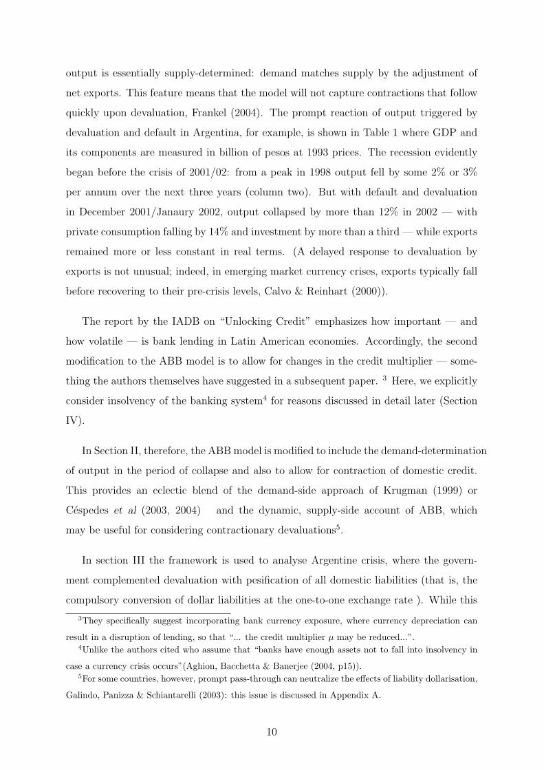
output is essentially supply-determined: demand matches supply by the adjustment of

net exports. This feature means that the model will not capture contractions that follow

quickly upon devaluation, Frankel (2004). The prompt reaction of output triggered by

devaluation and default in Argentina, for example, is shown in Table 1 where GDP and

its components are measured in billion of pesos at 1993 prices. The recession evidently

began before the crisis of 2001/02: from a peak in 1998 output fell by some 2% or 3%

per annum over the next three years (column two). But with default and devaluation

in December 2001/Janaury 2002, output collapsed by more than 12% in 2002 — with

private consumption falling by 14% and investment by more than a third — while exports

remained more or less constant in real terms. (A delayed response to devaluation by

exports is not unusual; indeed, in emerging market currency crises, exports typically fall

before recovering to their pre-crisis levels, Calvo & Reinhart (2000)).

The report by the IADB on “Unlocking Credit” emphasizes how important — and

how volatile — is bank lending in Latin American economies. Accordingly, the second

modification to the ABB model is to allow for changes in the credit multiplier — some-

thing the authors themselves have suggested in a subsequent paper. 3 Here, we explicitly

consider insolvency of the banking system4 for reasons discussed in detail later (Section

IV).

In Section II, therefore, the ABB model is modified to include the demand-determination

of output in the period of collapse and also to allow for contraction of domestic credit.

This provides an eclectic blend of the demand-side approach of Krugman (1999) or

Cespedes et al (2003, 2004) and the dynamic, supply-side account of ABB, which

may be useful for considering contractionary devaluations5.

In section III the framework is used to analyse Argentine crisis, where the govern-

ment complemented devaluation with pesification of all domestic liabilities (that is, the

compulsory conversion of dollar liabilities at the one-to-one exchange rate ). While this

3They specifically suggest incorporating bank currency exposure, where currency depreciation can

result in a disruption of lending, so that “... the credit multiplier µ may be reduced...”.4Unlike the authors cited who assume that “banks have enough assets not to fall into insolvency in

case a currency crisis occurs”(Aghion, Bacchetta & Banerjee (2004, p15)).5For some countries, however, prompt pass-through can neutralize the effects of liability dollarisation,

Galindo, Panizza & Schiantarelli (2003): this issue is discussed in Appendix A.

10

policy essentially eliminated the potential balance sheet effect for non-financial firms,

for banks — which had to convert their dollar liabilities at a higher rate — it proved a

paralyzing blow. We discuss how pesification can, in principle, mitigate adverse balance

sheet effects; but how it can plunge the economy into chaos if it precipitates a credit

crunch. In Section IV the Argentine pesification is compared and contrasted with the

historical precedent of President Roosevelt’s cancelation of the gold clause before the US

left the gold standard. After a brief discussion of capital flight and missed opportunities

for alternative policies in the Argentine case in section V, the paper concludes.

II An eclectic model of financial crisis

II.1 ABB’s supply-side model: a brief outline

The macroeconomic model of ABB is designed to capture the balance sheet effect on

private sector investment of an exchange rate collapse in a small open economy. Before

indicating our modifications, we briefly outline the central elements of this widely-cited

two-period model.

There is full capital mobility and uncovered interest parity holds. Purchasing Power

Parity (PPP) for traded goods also holds except in period 1 when an unanticipated shock

leads to a deviation as prices are preset, but other variables — the nominal exchange

rate in particular — are free to adjust. The actual timing of the events in period 1 is:

first the price of traded output is pre-set according to the ex ante PPP condition and

firms invest; then there is an unanticipated shock, followed by the adjustment of interest

rate and the exchange rate; finally, output and profits are generated, with a fraction of

earnings retained after debt repayment saved for investment in period 2. This determines

the level of production in the second period, when there are no shocks and prices are

flexible, so PPP is restored.

Equilibrium can be summarized by the intersection of two schedules, called the IPLM

curve and the W curve. The former, as the name suggests, is a combination of the

Uncovered Interest Parity, money market equilibrium and the PPP condition for the

11

second period. Formally, it is written as:

E1 =1 + i∗

1 + i1

MS2

L(Y2, i2)(1)

where E1 is the exchange rate for the first period, i∗ is the foreign interest rate, i1 and i2

are domestic interest rates for periods 1 and 2, MS2 and Y2 are money supply and output

in period 2, and L(Y2, i2) is the money demand function. This IPLM curve is downward

sloping in the E1 and Y2 space because higher output in the second period increases

money demand (i.e., higher L given interest rate in period 2) and so strengthens the

exchange rate (note MS2 is given).

The W -curve characterizes the supply of output on the assumption that entrepreneurs

are credit-constrained. (The production function is assumed to be linear in capital stock,

which depreciates completely at the end of the period.) Total investment consists of

last-period retained earnings together with borrowing (in both domestic and foreign cur-

rencies, with proportions given exogenously) which is limited to a given fraction µt(it−1)

of retained earnings. The credit multiplier µt(it−1), with µ′t < 0, is designed to capture

the imperfection of the credit market. The W -curve is specifically given by

Y2 = σ[1 + µ2(i1)](1− α)

[Y1 − (1 + r0)D

C − (1 + i∗)E1

P1

(D1 −DC)

](2)

where σ is a productivity parameter, α is the fraction of output consumed in each period,

D1 is total borrowing in period 1, and DC is its domestic currency component. Because

currency depreciation increases the burden of corporate debt and reduces next-period

output, the W-curve is downward sloping in E1 and Y2 space.6 Clearly this formulation

captures the contractionary effect of devaluation on the supply-side. Next we discuss

two major modifications proposed — a fall of demand below supply immediately after

devaluation and a contraction in the credit multiplier.

II.2 Demand-determined output and a credit crunch

An unexpected currency collapse in period 1 lowers output in period 2 in the ABB model:

but it leaves output in period 1 unchanged. As noted earlier, Argentine GDP collapsed

6Note that Y2 is set to zero if the right hand side of (2) turns out to be negative, where Y2 = 0

signifies the depression level of output.

12

at the same time as the currency, with investment showing the largest percentage fall.

The simplest way to capture this while retaining other features of the model is to assume

what is shown in Table 1, namely that export volumes remain unchanged — a modest

assumption given the finding of Calvo & Reinhart (2000) that, in case of an emerging

market currency crisis, exports typically fall before recovering to their pre-crisis levels

after 8 months: and, with a banking crisis, exports may need 20 months to recover.

A consideration relevant in the Argentine case is discussed in Kohlscheen & O’Connell

(2004), namely the restriction of trade credit by external creditors faced with default

on sovereign debt: it is in their strategic interest to limit the expansion of exports as a

sanction in restructuring negotiations.7

As a consequence of taking export volumes as given, output in period 1 may be is

demand-determined, i.e., the fall of investment can cut current output and consumption.

Specifically, let output in period 1 be determined as follows:

Y Dt = γα(Yt −D∗

t ) + (1 + µt+1)(1− α)(Yt −D∗t ) + X −mYt, (3)

where D∗1 = (1 + r0)D

C +(1+ i∗)(E1/P1)(D1−DC) is the total cost of debt services and

Yt is aggregate demand measured in constant prices. In support of this specification, note

that, in the midst of a credit crunch and bank closures, both consumers and producers

were effectively denied access to new credit. The first term on the right hand side of (3)

indicates consumption demand where α < 1 is the labor share of income and γ < 1 is the

fraction spent on consumption. The second term is demand for investment with Yt−D∗t

representing corporate profits net of borrowing costs, and µ is the credit multiplier. The

last two terms represent net exports, where we assume export volumes are fixed in the

current period while imports vary proportionally with current income – as the data above

suggest is broadly appropriate. The failure of export volumes to rise means that a collapse

of investment (due to balance sheet effects, for example) can reduce realized output in

the current period, as well as supply potential in the next period.

7Other factors include contract lags and physical capacity constraints: the export response to the

spectacular fall of the Indonesian currency in 1997/98 was considerably hampered by lack of container

shipping capacity, for example.

13

Solving (3) for period 1 yields

Y D1 =

−D∗1[γα + (1 + µt+1)(1− α)] + X

1 + m− [γα + (1 + µt+1)(1− α)],

=−ξD∗

1 + X

1− ξ + m< Y S

1 , (4)

where ξ = γα + (1 +µt+1)(1−α) and 1 > 1− ξ + m > 0, and Y S1 is the aggregate supply

in the same period. The Keynesian-style multiplier on exports is simply 1/(1− ξ + m),

where ξ is the marginal propensity to spend and 1− ξ the marginal propensity to save.

Output

Exchange rate

C

Yd

Aggregate supply

E0

AE1 B

Aggregate demand

Balance sheet

effect

Y1

Devaluation

Credit crunch

Pesification

Figure 1: Aggregate demand and supply in period 1.

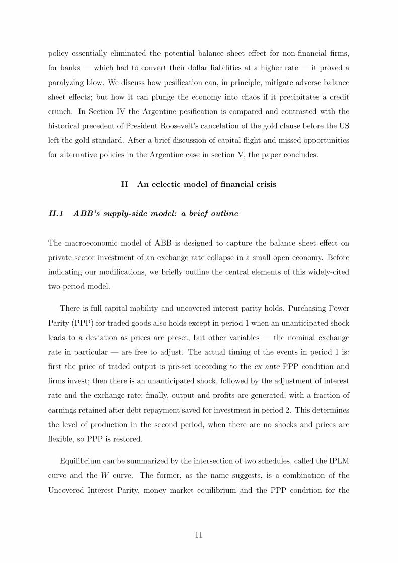
Figure 1, with output on the horizontal axis and the exchange rate on the vertical,

illustrates how demand failure can lead to prompt contractionary devaluation in the ABB

model. Since it depends on output and interest rate in the previous period, aggregate

supply appears as a vertical line Y S1 . Aggregate demand, however, moves inversely with

the exchange rate due to the adverse balance sheet effects of a devaluation which raises

the price of a dollar from E0 to E1. At E1 for example, demand has fall by AB as a

result. (The reduction of investment — not shown here — will of course reduce future

14

potential output.) If, however, devaluation is accompanied by pesification, the aggregate

demand effect will be eliminated, as indicated by the arrow in the figure: in the case of

Argentina, for example, “the pesification ... of all domestic liabilities that followed the

January 2002 devaluation all but eliminated any potential balance sheet effect” Galiani,

Levy-Yeyati & Schargrodsky (2003, p.344). 8 But if devaluation and pesification lead

to a credit crunch, the reduction in the credit multiplier in equation 3 will shift the

aggregate demand schedule to the left, as shown by the dotted line: so output falls to C

at E1. (An increase in the period 1 interest rate will also shift Y D1 leftwards and flatten

it as high interest rates reduce the credit multiplier and investment demand.)

Table 2: Comparison with the ABB model.

ABB model MFZ modification

Y1 Y s1 = σ[1 + µ1(i0)](1− α)[Y0 −D∗

0] Y D1 = [γα+(1+µ2)(1−α)]×[Y1−

D∗1] + X −mY1

Y1 = Y s1 = Y D

1 Y1 = Y D1 < Y s

1 = Y s1 (ABB)

Y2 Y s2 = σ[1 + µ2(i1)](1− α)[Y1 −D∗

1] Y D2 = Y s

2 < Y s2 (ABB)

Table 2 compares and contrasts the determination of output when the quantity of

exports cannot adjust within period to maintain the balance of demand with supply

with that of the standard ABB model where output is supply-determined (as indicated

in the first column). For the latter, an adverse devaluation-induced shock to the balance

sheet in period 1 has no effect on period 1 output (which is determined by previous period

investment), but reduces period 2 output through reduced capital accumulation.

The table can also be used to show how a credit crunch may have an impact on

current-period output. Consider, for example, a contraction in the credit multiplier

µ2 due to asymmetric pesification leading to bank closures in period 1. In the ABB

model, the impact on output is delayed until period 2 as can be seen from column 1

(which is presumably why the credit multiplier carries the label 2). With Keynesian

demand determination, however, the effects are more immediate and more damaging.

The tightening of corporate credit constraints reduces investment in period 1 directly:

8With partial pesification which reduces corporate dollar debt to E1 > E0, the demand curve will

become vertical at a lower level of aggregate demand

15

but this exogenous fall in demand triggers a contraction of income in period 1, which in

turn leads to even less investment as profits fall. The knock-on effect on period 2 supply

is consequently greater than in the ABB model.9

How adding Keynesian demand in period 1 alters a key policy implication of the ABB

model, may be summarized as follow:

Proposition 1 If output in period 1 is demand-determined, as specified in (4), an in-

crease in the period 1 interest rate will weaken the domestic currency relative to when

output is supply determined.

Proof: As noted above, the equilibrium of (Y2, E1) is given by the intersection of (1) and

(2) with Y1 in (2) being replaced by Keynesian demand given in (4). The proposition is

true if an increase in i1 induces more leftward shift to Y2 in our specification than that

in the ABB’s, i.e.,

∂Y2

∂i1

MFZ

<∂Y2

∂i1

ABB

. (5)

Differentiating Y2 in (2) with respect to i1 (with Y1 replaced by Y D1 from (4)) yields

∂Y2

∂i1

MFZ

=µ′2(i1)

1 + µ2(i1)Y2 + σ(1 + µ2)(1− α)

∂Y D1

∂i1.

where the first term on the left hand side is what we would have obtained if we use

ABB specification, and the second term gives the additional effect because the output

in period 1 is demand determined. As is clear from (4) that ∂Y D1 /∂i1 < 0, so (5) must

hold.

In table 2 and the analysis below, we follow ABB in assuming that output in period 2 is

supply-determined. This does not mean that output in period 2 matches that of the ABB

model, however: the contraction is greater because of the reduced investment associated

with the fall in aggregate demand in period 1. (The simplifying assumption made by

ABB that capital depreciates completely within one period dramatically highlights this

effect, but is surely an exaggeration.) Of course, if exports fail to respond sufficiently

promptly, output may also fall below supply in period 2 as well.

In Appendix A we discuss the pass-through of the exchange rate on to the price level

9Cutting µ1, credit multiplier corresponding to period 0, would, however, have same effects on period

1 supply in both models.

16

and how this could, in principle, offset adverse balance sheet effects. For Argentina, we

conclude that this is not the case.

III Analysing the Argentine crisis

In this section the modified ABB model is used to help explain how “Argentina passed

from being one of the world’s fastest growing economies in the 1990s to suffering one

of the sharpest recessions of any peace-time capitalist economy since the Second World

War” (Gerchunoff & Llach 2003, p.456). For this purpose it is convenient to identify the

three separate periods as follows: Pre-collapse (approximately 2001); Currency Collapse

and Depression (approximately 2002 ); Continued Depression (2003), which are referred

to as Period 0, 1 and 2 respectively. For reference, inter-bank interest rates from the

beginning of 2000 to September 2004 are shown in Figure 2 (monthly average of the

BAIBOR 30 days in pesos: data for Dec 2001, Jan 2002 are not available).

Figure 2: Inter-bank rates in Argentina from Jan 2001 to Sep 2004

(Source: Banco Central de la Republica Argentina.)

17

III.1 The end of Convertibility and the prospect of economic collapse

The proximate trigger for the end of convertibility was the IMF announcement in De-

cember 2001 that the country would not receive the $1.3 bn of financial support that

the government had requested to cover debt payments (Blustein 2005, Prologue and

pp.181ff.). When the denial of financial support led to restrictions on the withdrawal of

bank deposits, there was a rapid spread of street demonstrations, looting of supermarkets

and a general strike, and domestic turmoil forced De la Rua to resign the presidency on

the 20th of December, leaving the country in constitutional chaos with three successive

presidents elected by the Congress in quick succession. Political stability was partially

regained at the beginning of January 2002 when Eduardo Duhalde was appointed as the

new president. One of his first economic measures was the devaluation of the peso. It

fell far more than anticipated: instead of rising to 1.4 as planned, the price of a dollar

climbed to over 3 pesos. The economy as a whole promptly fell into recession, and output

remaind below its level in 2001 for two years (as can be seen in Table 1 above).

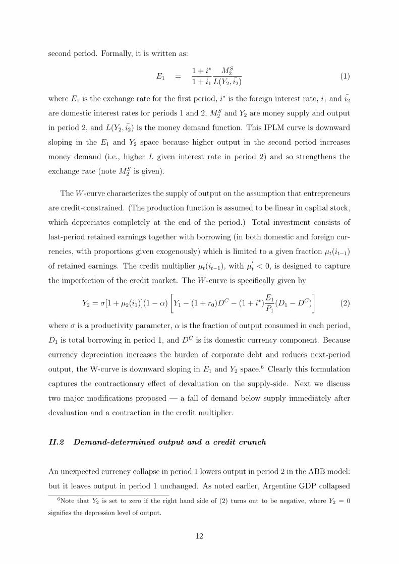
To understand the sequence of events that led to currency and output collapse we

manipulate the IPLM and W schedules. (Note that, as in ABB, the axes here are the

exchange rate in period 1 and output the following period: the behavior of output in

period 1 when the currency collapses will be discussed in the text). We start in period

0, where Cavallo’s last-ditch attempts to maintain the dollar peg were associated with

punishingly high interest rates and low investment. With the peg still in place, the IPLM

curve is not relevant, its place being taken by the parity peg. The high interest rates

shift the W-curve leftwards, however, decreasing potential output in period 2 from A to

B, see Figure 3 and Appendix B which analyses forces of contraction under the dollar

peg.

Next consider period 1 when the peso was floated and interest rate increased sharply

(see Figure 2). The higher cost of credit would shift the W further left, decreasing

potential output from B to B′ were the peso still at parity with the dollar. Assuming,

however, that monetary policy was expected to accommodate a modest devaluation, the

IPLM curve is drawn intersecting the W curve at C, with the dollar rising from E0 to

E1 and the IPLM intersecting the W curve at C. (Note that the “indexation” of 40% of

18

Y2

E1

W

IPLM

E0

Yd

C

Peg to the dollar

Ē1

B A' AWF

Figure 3: Demand failure and the risk of economic collapse.

deposits to the dollar ensured some nominal accommodation.)

Equilibrium at C requires that export volumes rise sufficiently to keep aggregate

demand equal to supply in period 1. With exports slow to react, however, devaluation

will be contractionary for output: and the knock-on effect of demand failure on potential

output in period 2 is captured by schedule WF in the figure. (Note that we assume no

demand failure in period 2.)

There may be no intersection with the IPLM curve until output falls to depression

level Yd and the price of the dollar rises sharply, as the figure suggests. This was the risk

of economic collapse facing the incoming administration.

19

Y2

E1

IPLM

E0

Yd

C

Peg to the dollar

BWF

1E)D

WF

WF

sp

ap

C'

D'

B'

Figure 4: Pesification and credit contraction: “Nuestra gran depresion”?

III.2 Imitating President Roosevelt

To mitigate or avoid depression, the government attempted to follow the example of

President Roosevelt; and the potential effect of so doing is indicated in Figure 4. Consider

first the pesification of corporate borrowing which has no negative effect on the solvency

of the banking system (e.g., symmetric pesification when loans and deposits are both

pesified at a rate of E1, for example). In this case, for values of the dollar greater than

E1, the W F -curve rotates clockwise to become vertical at E1 , see Appendix C; and the

new equilibrium is given by the intersection of W FSP with the IPLM curve, at point C ′.

This Rooseveltian policy of pesification prevents output from collapsing because it affords

across-the-board relief to corporations with dollar debts, along the lines advocated by

Joseph Stiglitz in his proposal for a Super-Chapter 11, Stiglitz (1999), Miller & Stiglitz

(1999). But this equilibrium still involves some demand failure and the contraction of

future supply. Giving borrowers even more relief – by pesifying all dollar loans below

20

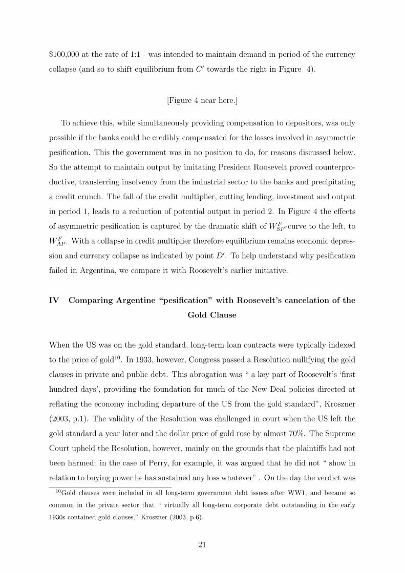
$100,000 at the rate of 1:1 - was intended to maintain demand in period of the currency

collapse (and so to shift equilibrium from C ′ towards the right in Figure 4).

[Figure 4 near here.]

To achieve this, while simultaneously providing compensation to depositors, was only

possible if the banks could be credibly compensated for the losses involved in asymmetric

pesification. This the government was in no position to do, for reasons discussed below.

So the attempt to maintain output by imitating President Roosevelt proved counterpro-

ductive, transferring insolvency from the industrial sector to the banks and precipitating

a credit crunch. The fall of the credit multiplier, cutting lending, investment and output

in period 1, leads to a reduction of potential output in period 2. In Figure 4 the effects

of asymmetric pesification is captured by the dramatic shift of W FSP -curve to the left, to

W FAP . With a collapse in credit multiplier therefore equilibrium remains economic depres-

sion and currency collapse as indicated by point D′. To help understand why pesification

failed in Argentina, we compare it with Roosevelt’s earlier initiative.

IV Comparing Argentine “pesification” with Roosevelt’s cancelation of the

Gold Clause

When the US was on the gold standard, long-term loan contracts were typically indexed

to the price of gold10. In 1933, however, Congress passed a Resolution nullifying the gold

clauses in private and public debt. This abrogation was “ a key part of Roosevelt’s ‘first

hundred days’, providing the foundation for much of the New Deal policies directed at

reflating the economy including departure of the US from the gold standard”, Kroszner

(2003, p.1). The validity of the Resolution was challenged in court when the US left the

gold standard a year later and the dollar price of gold rose by almost 70%. The Supreme

Court upheld the Resolution, however, mainly on the grounds that the plaintiffs had not

been harmed: in the case of Perry, for example, it was argued that he did not “ show in

relation to buying power he has sustained any loss whatever” . On the day the verdict was

10Gold clauses were included in all long-term government debt issues after WW1, and became so

common in the private sector that “ virtually all long-term corporate debt outstanding in the early

1930s contained gold clauses,” Kroszner (2003, p.6).

21

announced, corporate bonds whose gold clause was abrogated rose in price – evidence,

it appears, that cancelation promised a better return than enforcement, Kroszner (2003,

p.22).

This historical precedent led some observers11 to recommend devaluation-with-pesification

as an appropriate policy option for Argentinain 2001; and Blustein (2005, p.142,3) in-

dicates that economists in the IMF Research Department also backed devaluation-with-

default as a better option than borrowing more to defend peso parity with the dollar12.

When the Convertibility regime ended in January 2002, President Duhalde of Argentina

did in fact ‘pesify’ debt contracts, and Roosevelt was explicitly cited as a precedent,

Rodriguez-Diez (2003, p.89). In the analysis that follows, however, we argue that the

process of pesification, rather than helping to ameliorate the crisis as in the US, may have

played a key role in its propagation. This prompts the immediate question: what was so

different between these two cases? Kroszner (2003, p.4 and p.28) indicates two factors:

first unlike the US, the Argentine government engaged in ‘asymmetric’ pesification; and

second that Argentina may have suffered more from the lack of respect for the rule of law

involved in such across-the-board abrogation of contracts. These issues are considered in

more detail, before proceeding with the formal model.

IV.1 Bank balance sheets and asymmetric pesification

Abrogation in the US affected only long-term bonds: it did not involve short-term loans

and deposits; and it did not precipitate bank insolvency. In fact, US commercial banks,

which would have made a substantial capital gain from the operation of the gold clause13,

had the prospective increase in their net worth anulled by the Act of Congress. So, for

the balance sheets of US banks, dollar devaluation was a ‘wash’.

Not so in Argentina. To begin with, the dollar-denomination of banking system assets

was much more extensive than gold-indexation of bank assets had been in US, for it

11e.g. Hausmann (2001), Miller (2001).12Specifically Ken Rogoff and Carmen Reinhart.13With more than 20% of their portfolios invested in long term securities, a 70 percent increase in the

value of these investments could have added almost about 15% to their net worth (normally about 12%

of their assets).

22

included bank loans as well as investments, and amounted to almost half of all assets. As

it was broadly matched by liability dollarisation — with half of all deposits denominated

in the US currency — devaluation-with-pesification could have been a wash for bank

balance sheets too; and it could have been economically beneficial, serving “ to protect

banks from devaluation, inasmuch as to have maintained deposits and loans in dollars

would have made it very difficult to recover loans in sufficient volume to honor deposits”

Sturzenegger (2003, p.49). But political imperatives led to the policy of asymmetric

pesification, which exacerbated balance sheet problems for the banks.

The reasons for adopting this policy - and some of its immediate consequences - are

graphically described in Blustein (2005, p.192,3):

To head off mass bankruptcy, the government decreed that most people who had

borrowed in dollars could repay their loans in depreciated pesos, at the rate of one

peso per dollar. At the same time, to appease savers, the authorities announced

deposits would be converted at a different rate - 1.4 pesos per dollar. As a result,

the banking system, which was already on its knees, was rendered prostrate. The

disparity between what banks could collect from their borrowers, and what they

owed their depositors, added up to billions of dollars in new losses. So for people

and businesses in need of credit, obtaining bank loans became all but unthinkable.

As for depositors, they felt cheated, notwithstanding the concession the government

had given them. . . Their angry reaction led to a deepening of the banking system’s

woes, as thousands of them obtained court orders requiring the return of their

deposits in full, and money began draining anew from the banking system. . .

[T]he economy headed into another downward spiral when the government, having

encountered resistance in Congress against a proposal straighten out the bank-

ing mess, closed the banks and exchange houses on April 19 [2002]. . . When the

banks reopened a week after the closure, they were still not lending; how could

they, bankers asked, when they had no idea of how many depositors would win

court orders, and could not even prepare meaningful statements of their financial

condition.

Asymmetric pesification implied losses of 40% on about 30% of banks’ portfolios

(on the optimistic assumption that government debt would pesified at the same rate as

23

deposits) – enough to wipe out bank capital of about 12 percent, see Miller, Garcıa-Fronti

& Zhang (2005).

IV.2 Credibility of the Government

In fact the Duhalde government promised from the outset that it would recapitalize bank

losses in the form of government bonds, Rodriguez-Diez (2003, pp109-10). This brings us

to the second crucial difference between the two cases: the standing of the government.

The cancelation of the gold clause was a pre-emptive measure taken by an administration

credible enough to borrow at interest rates of less than one percent to finance deficits of

around 8 percent of GDP14; and it was soon to be followed by the creation of the FDIC

to protect banks from panic. In Argentina, by contrast, pesification was pursued in the

throes of political turmoil and self-fulfilling panic in capital markets. By August 2001,

with the economy contracting and sovereign spreads reaching 1000 points, it appeared

that debt dynamics were unsustainable, leading to high level discussions with the IMF

about forcible sovereign debt restructuring15; and, by the time Duhalde took office in

January 2002 to complete the term left unfinished by De la Rua, sovereign bonds were

in outright default.

Not only were the assets offered to the banks by way capital restructuring of uncertain

value, but the ‘test of harm’ used by the US Supreme Court was not applicable as many

banks were foreign owned: for them, maintenance of peso values would not preserve their

purchasing power16.

Finally we note that commercial banks in Argentina were left free to export dollars

unchecked until newly-borrowed foreign currency reserves were exhausted, but in the US

pre-emptive cancelation of the gold clause was promptly followed an executive order of

the President mandating the surrender of gold to the Treasury and the Federal reserve

14In 1934, for example, when GDP was approximately $50bn the deficit was $4bn.(Statistics abstract

of the United States, Bureau of Census Library)15Talks between Cavallo and the IMF in October 2001 aimed at securing an involuntary 30 to 40

percent write down of sovereign debt apparently foundered because they threatened bank insolvency,

Blustein (2005, pp168,9).16This theme is explored in Miller, Garcıa-Fronti & Zhang (2005), treating bank recapitalization in a

strategic setting where domestically-owned banks will accept bonds but not foreign multinationals.

24

Banks, Kroszner (2003, p.7). Surprising as it may sound, private holding of gold in the US

for any other purpose besides ornamentation or industrial use was effectively prohibited

until this directive was revoked fifty years later.

V Policy alternatives

With time, the economy is on a recovery path; the government is paying compensation to

the banks; sovereign debt has been restructured; and sovereign spreads have fallen below

5% in the summer 2005. But the fact that “ the economic collapse that accompanied

Argentina’s eventual default and devaluation was much deeper than necessary to bring

Argentina’s external accounts into some semblance of balance ... suggests it is at least

conceptually possible that an alternative policy path might have produced a smaller fall

in output.” Roubini & Setser (2004, p.355). What alternative policies might have

helped?

The comprehensive review of financial conditions and crises in Latin America carried

out by the IADB focuses on bank restructuring. Noting that “the initial measures taken

by the authorities in Argentina aggravated rather than improved the solvency of banks”,

they criticize the authorities because they “did not put in place a serious and compre-

hensive program for bank restructuring... and did not discriminate int the treatment of

bank according to quality” (in contrast to Uruguay were “credible funds” were secured

to finance the implementation of a comprehensive restructuring program), IADB (2004,

p.80). A government itself facing a solvency crisis will inevitably face great difficulty in

restoring bank solvency: one must surely look for action that could been taken earlier to

forestall or minimise crisis.

Note that Roosevelt took pre-emptive action nine months before devaluing, by can-

celing the gold clause and imposing capital controls to conserve US gold reserves. But in

Argentina there were no capital controls until December 2001. The capital account was

left open — with capital flight estimated at $23 bn in 2000-1, Bonelli (2004, p.216). So,

despite IMF loans in early and mid-2001, official reserves ran down sharply, falling by

$20 billion between October 2000 - when the political crisis began with the resignation

of Vice President Alvarez - until the end of 2001, Bonelli (2004, p.215). The model of

25

Caballero & Krishnamurthy (2001) – where capital flight leads to output contraction

via the loss of internationally acceptable collateral underpinning corporate borrowing –

seems to provide a convincing rationale for outflow controls, at least on a temporary ba-

sis17. That such measures were not considered is no mystery: the late 1990s was the high

water mark for the fashion of prompt and comprehensive liberalization, and Argentina

was one of its leading exponents.

How would action to restrict outflows on capital account impact on the exchange

rate and output in ABB model used here? In principle, it would move the IPLM curve

down sufficiently to intersect the W ′′-curve, helping to avoid the precipitate collapse of

output18. In addition, the protection so afforded to government solvency could have made

a bank bailout more credible and prevented the collapse of the credit multiplier.

Absent capital controls, however, it seems clear that the Convertibility regime should

have been ended earlier, certainly before the IMF agreed the second disbursement of

funds in August/September 2001 in the view of Mussa (2002, pp.45-48): of this decision

he remarks “Argentina was not helped. Indeed, external assistance that was potentially

far more valuable in helping to contain the damage once a de facto sovereign default had

occurred was instead squandered in a futile effort to avoid the inevitable.” Roubini and

Setser (2004, p.354) also criticize the policy followed by the IMF , whereby “ Argentina . . .

ended up receiving a significant loan to support an attempt to avoid both any exchange

rate adjustment and meaningful debt reduction but nothing to support a transition to

a sustainable real exchange rate and a more sustainable debt profile” . Why the fateful

delay? Could it reflect perverse domestic incentives for economic management?

Cooper (1971) has noted that finance ministers typically lose their jobs after deval-

uation — and governments often fall as well. If the end of convertibility was seen as

tantamount to political failure, the administration would have been sorely tempted to

17The case for inflow controls, like those used in Chile, has been made by Levy Yeyati (2005) – both

as a preemptive measure to avoid the rapid build-up of speculative dollar liabilities and so that, in an

panic, less-than-one-year investors cannot exit with all their assets.18Technically one can modify the IPLM curve to

E1 = (1− c)1 + i∗1 + i1

MS2

L(Y2, i2)

where 0 < c < 1 indicates the degree of capital controls, see Aghion, Bacchetta & Banerjee (2001).

26

‘gamble for resurrection’, taking great risks with the country’s future so as to defend the

parity rather than looking at the expected economic costs and benefits of policy options.

This interpretation of Argentine policy-making is attributed to Ken Rogoff who, when

appointed chief economist at the IMF, argued against further lending in favor of deval-

uation and default — followed by IMF support , Blustein (2005, p.142). On this view,

distorted political incentives may well have promoted delay, and IMF loans financed it.

VI Conclusions

Devaluation in emerging markets often leads to economic contraction, and in the Argen-

tine case the end of Convertibility led to veritable economic collapse. In this paper we

show how balance sheet models of crisis may be used to throw light on the issue.

After devaluation and default, the Argentine government tried to protect producers

by a policy of asymmetric pesification which, in the absence of credible capitalization,

bankrupted the banking system. Suitably adapted, the framework of Aghion, Bacchetta

& Banerjee (2000) illustrates how high ex ante interest rates can have substantial adverse

effect on the supply side and how asymmetric pesification of bank assets can — via a

credit crunch — greatly exacerbate the fall of the currency and the depth of the recession.

The speed of collapse and the level of unused resources implies that, as for the 1930s,

one needs to model demand as well as supply: and the model is modified to do just this.

An issue for further investigation (briefly discussed in Appendix A) is the difference

between traded and non-traded sectors in the rate of “pass-through”. We note that the

analysis of Carranza, Galdon-Sanchez & Gomez-Biscarri (2005), where “pass-through”

in the latter case depends on the state of the economy, are broadly consistent with the

account of collapse developed in this paper. 19

Failure to replicate the successful cancelation of gold clause by President Roosevelt can

be attributed to greater “dollarisation” of the economy and the serious loss of credibility

by the quick succession of presidents appointed in the midst of the crisis. So we conclude

that preemptive measures taken earlier in 2001 were needed to avoid disaster. But

19Their interesting analysis takes no account of singular aspects of the Argentine case considered here,

however, i.e. asymmetric pesification and credit collapse.

27

preemptive measures required policy agreement between the IMF and the Argentine

government on how to end convertibility. Could this episode have revealed an Achilles

heel in the IMF policy of helping countries which help themselves — an agency problem

which postpones corrective action until disaster is all but inevitable? The way in which

strategic policy decisions involving the IMF are arrived at before and during such crises

could repay further investigation.

28

VII *

References

Aghion, Philippe, Philippe Bacchetta & Abhijit Banerjee (2000), ‘A simple model of

monetary policy and currency crises’, European Economic Review 44(4-6), 728–738.

Aghion, Philippe, Philippe Bacchetta & Abhijit Banerjee (2001), ‘Currency crises and

monetary policy in an economy with credit constraints’, European Economic Review

45(7), 1121–1150.

Aghion, Philippe, Philippe Bacchetta & Abhijit Banerjee (2004), ‘A corporate balance-

sheet approach to currency crises’, Journal of Economic Theory 119, 630.

Blejer, Mario (2005), Managing argentina’s 2002 financial crisis, in T.Besley &

N. R.Zagha, eds, ‘Development Challenges in the 1990s: Leading Policymakers

Speak from Experience’, World Bank.

Blustein, Paul (2005), And the Money Kept Rolling in (and Out): Wall Street, the IMF

and the bankrupting of Argentina, first edn, Public affairs, New York.

Bonelli, Marcelo (2004), Un Paıs en Deuda, 1a edn, Planeta, Buenos Aires.

Burstein, Ariel, Martin Eichenbaum & Sergio Rebelo (2004), ‘Large devaluations and the

real exchange rate’, 2004 Meeting Papers from Society for Economic Dynamics.

Caballero, Ricardo & Arvind Krishnamurthy (2001), ‘Interantional and domestic col-

laretal constraints in a model of emerging market crises’, Journal of Monetary Eco-

nomics (48), 515–548.

Calvo, Guillermo A., Alejandro Izquierdo & Ernesto Talvi (2003), ‘Sudden stops, the real

exchange rate, and fiscal sustainability: Argentina’s lessons’, NBER Working Paper

No. w9828.

Calvo, Guillermo & Carmen Reinhart (2000), When capital inflows come to a sudden

stop: Consequences and policy options, in P.Kenen & A.Swoboda, eds, ‘Key Issues

in Reform of the International Monetary and Financial System’.

29

Carranza, L., Jose E. Galdon-Sanchez & Javier Gomez-Biscarri (2005), ‘Exchange rate

and inflation dynamics in dollarized economies’, Mimeo University of Navarra. Con-

ference paper.

Cespedes, Luis, Roberto Chang & Andres Velasco (2003), ‘IS-LM-BP in the Pampas’,

IMF Staff Papers 50(Special issue), 143–156.

Cespedes, Luis, Roberto Chang & Andres Velasco (2004), ‘Balance sheets and exchange

rate policy’, American Economic Review 94(Special issue), 1183–1193.

Cooper, Richard (1971), ‘Currency devaluation in developing countries’, Essays in Inter-

national Finance (86), 276–304. Princeton, NJ: Princeton University.

Escude, Guillermo J. (2004), ‘Dollar strength, peso vulnerability to sudden stops: A

perfect foresight model of Argentina’s convertibility’, mimeo, Banco Central de la

Republica Argentina.

Frankel, Jeffrey A. (2004), ‘Contractionary currency crashes in developing countries’,

Presented at The 5th Mundell-Fleming Lecture IMF Annual Research Conference.

Conference paper.

Galiani, Sebastian, Eduardo Levy-Yeyati & Ernesto Schargrodsky (2003), ‘Financial dol-

larization and debt deflation under a currency board’, Emerging Markets Review

4(4), 340–367.

Galindo, Arturo, Ugo Panizza & Fabio Schiantarelli (2003), ‘Debt composition and bal-

ance sheet effects of currency depreciation: a summary of the micro evidence’,

Emerging Markets Review 4(4), 330–339.

Gerchunoff, Pablo & Juan Llach (2003), El Ciclo de la Ilusion y el desencanto, 1a edn,

Ariel, Buenos Aires.

Hausmann, Ricardo (2001), ‘A way out for Argentina’, Financial Times. London.

IADB (2004), Unlocking credit. economic and social progress in Latin America: 2005

report., Technical report, IADB, Washington DC.

Kohlscheen, Emmanuel. & Steve A. O’Connell (2004), ‘A sovereign debt model with

trade credit and reserves’, Mimeo.

30

Kroszner, Randall (2003), ‘Is it better to forgive than to receive? an empirical analysis

of the impact of debt repudiation’, mimeo, University of Chicago November.

Krueger, Anne & Matthew Fisher (2003), ‘Building on a decade of experience: Crisis pre-

vention and resolution’, Paper presented at “International Financial Crises: What

Follows the Washington Consensus?”. Warwick University.

Krugman, Paul (1999), Balance sheets, the transfer problem, and financial crises, in

P.Isard, A.Razin & A. K.Rose., eds, ‘International Finance and Financial Crises:

Essays in Honor of Robert P. Flood’.

Levy Yeyati, Eduardo (2005), ‘Tras el canje de deuda vuelve el control de capitales version

2005’, Cronista Comercial. Buenos Aires. 26 Febrary.

Miller, Marcus (2001), ‘Argentina should look to Roosevelt’, Financial Times. London.

Sep 10, p.20.

Miller, Marcus, Javier Garcıa-Fronti & Lei Zhang (2005), ‘Credit crunch and keynesian

contraction: Argentina in crisis’, CEPR Discussion Paper No.: 4889. London, Centre

for Economic Policy Research.

Miller, Marcus & Joseph Stiglitz (1999), ‘Bankruptcy protection against macroeconomic

shocks: The case for a ’super chapter 11”, Unpublished manuscript presented at the

World Bank Conference on Capital Flows, Financial Crises and Policies, April 1999.

Mussa, Michael (2002), ‘Argentina and the Fund: From triumph to tragedy’, Policy

Analyses in International Economics No. 67, IIE, Washington D.C.

Powell, Andrew (2003), Argentina’s avoidable crisis: Bad luck, bad economics, bad pol-

itics, bad advice, in S. M.Collins & D.Rodrik, eds, ‘Brookings Trade Forum 2002.

Currency Crises: What Have We Learned?’.

Rodriguez-Diez, Alejandro (2003), Devaluacion y pesificacion, Bifronte Editores, Buenos

Aires.

Roubini, Nuriel & Brad Setser (2004), Bailouts or Bil-ins? Responding to Financial

Crises in Emerging Economies, 1 edn, Institute for International Economics, Wash-

ington DC.

31

Stiglitz, Joseph (1999), ‘Reforming the global economic architecture: Lessons from recent

crises’, The Journal of Finance (54), 1508–1521.

Sturzenegger, Federico (2003), La Economıa de los Argentinos, 1a edn, Planeta, Buenos

Aires.

32

Appendix

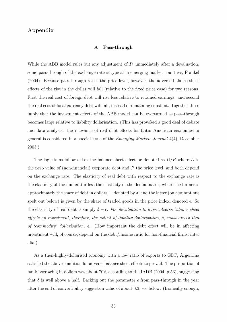
A Pass-through

While the ABB model rules out any adjustment of P1 immediately after a devaluation,

some pass-through of the exchange rate is typical in emerging market countries, Frankel

(2004). Because pass-through raises the price level, however, the adverse balance sheet

effects of the rise in the dollar will fall (relative to the fixed price case) for two reasons.

First the real cost of foreign debt will rise less relative to retained earnings: and second

the real cost of local currency debt will fall, instead of remaining constant. Together these

imply that the investment effects of the ABB model can be overturned as pass-through

becomes large relative to liability dollarisation. (This has provoked a good deal of debate

and data analysis: the relevance of real debt effects for Latin American economies in

general is considered in a special issue of the Emerging Markets Journal 4(4), December

2003.)

The logic is as follows. Let the balance sheet effect be denoted as D/P where D is

the peso value of (non-financial) corporate debt and P the price level, and both depend

on the exchange rate. The elasticity of real debt with respect to the exchange rate is

the elasticity of the numerator less the elasticity of the denominator, where the former is

approximately the share of debt in dollars — denoted by δ, and the latter (on assumptions

spelt out below) is given by the share of traded goods in the price index, denoted ε. So

the elasticity of real debt is simply δ − ε. For devaluation to have adverse balance sheet

effects on investment, therefore, the extent of liability dollarisation, δ, must exceed that

of ‘commodity’ dollarisation, ε. (How important the debt effect will be in affecting

investment will, of course, depend on the debt/income ratio for non-financial firms, inter

alia.)

As a then-highly-dollarised economy with a low ratio of exports to GDP, Argentina

satisfied the above condition for adverse balance sheet effects to prevail. The proportion of

bank borrowing in dollars was about 70% according to the IADB (2004, p.53), suggesting

that δ is well above a half. Backing out the parameter ε from pass-through in the year

after the end of convertibility suggests a value of about 0.3, see below. (Ironically enough,

33

as Galiani, Levy-Yeyati & Schargrodsky (2003) point out, the act of pesification reduced

the degree of liability dollarisation for non-financial firms immediately after the Argentina

peso was devalued: why this failed to rescue investment involves taking account of the

banking crisis as in Section IV.)

Burstein, Eichenbaum & Rebelo (2004) who construct an open economy general equi-

librium model that can account for the slow adjustment in non-tradable good prices after

a large devaluation estimate that consumer prices rose by about 40% in the first year in

response to a rise in the price of the dollar of more than 200%. As aggregate pass-through

will reflect the share of traded goods in the price index, we can back out the value of ε

on the simplifying assumption that there is complete pass-through for traded goods and

none for non-traded. Formally, let the aggregate price level (P ) be a weighted geometric

average of tradable (PT ) and non-tradable (PN) prices

P = P εT P 1−ε

N (6)

it follows thatPt

P0

=1.4

1=

(Et

E0

)ε

=

(3

1

)0.3

(7)

i.e. ε = 0.3.

An important factor being glossed over in this simple calculation is the sectoral vari-

ation in pass-through. This is analysed by Carranza, Galdon-Sanchez & Gomez-Biscarri

(2005) who assume traded goods are priced in dollars but pass-through in the non-traded

goods sector is endogenous: it depends on the state of the economy, with low pass-

through when demand is depressed. With devaluation large enough to trigger significant

bankruptcy, the prediction of their analysis is consistent with the model we use here: low

output and low pass-through. For an explicit two-sector analysis of the Argentine case,

see Escude (2004) .

B Contraction under the dollar peg

That economic recession led to higher not lower interest rates in the highly indebted

Argentine economy, and that recession was met with policies which increased tax and

decreased public expenditure are identified by Gerchunoff & Llach (2003, p456) as two

34

important ‘crisis propagation mechanisms’. These could be incorporated in the model as

follows.

Corporate Tax

Assuming that corporate tax is levied at a given rate of τ on the firm’s realized profits.

Introducing taxes reduces the investment in period 1, which in turn affects negatively

the output in period 2:

Y2 = σ(1 + µ)(1− α− τ)

[Y1 − (1 + r0)D

C − (1 + i∗)E1

P1

(D1 −DC)

]. (8)

Public debt

As in Aghion, Bacchetta & Banerjee (2001), the consolidated government financing

equation can be written as

Pt(gt−tt)+

[XG(1 + it−1) + (1−XG)(1 + i∗)

E1

Et−1

]dG

t Pt−1 = (dGt+1+st)Pt−Et∆Rt (9)

where gt and tt are real government expenditure and taxes, dGt is the government debt

held by private individuals in period t and XG is the fraction of its domestic component,

st is the real seignorage, Pt is price level at t. Dividing both sides of (9) by Pt and

omitting reserve changes yield

(gt − tt) +

[XG(1 + rt−1) + (1−XG)(1 + i∗)

E1

Pt

]dG

t = dGt+1 + st. (10)

Country risk

To capture the default risk for the dollar debt, we introduce risk premium to both

the interest paid by government (πG) and the interest rate paid by the firm (πP ). In the

presence of such risk premium, the government budget (10) constraint becomes

(gt − tt) +

[XG(1 + rt−1) + (1−XG)(1 + i∗ + πG)

E1

Pt

]dG

t = dGt+1 + st. (11)

The output in period 2 becomes

Y2 = σ(1 + µ)(1− α− τ)

[Y1 − (1 + r0)D

C − (1 + i∗ + πP )E1

P1

(D1 −DC)

]. (12)

Pre-collapse contraction of supply

35

The first contractionary mechanism identified by Gerchunoff and Llach is the high

sovereign spreads force the government to increase corporate tax to maintain the “zero

deficit” commitment with the IMF Blustein (2005, p.136 and p.138), as can be seen from

the following accounting equation from (11)

(gt− tt) +

[XG(1 + rt−1) + (1−XG)(1 + i∗ + πG)

E1

Pt

]dG

t = dGt+1 + st = Constant. (13)

where the first term is the primary deficit and the second term represents the interest

payment on public debt. Assuming that the sum of terms is fixed, the only way to

adjust to rising interest costs is to run a primary surplus — by raising corporate taxes

for example.

The second mechanism is the high credit risk πP (risk over American companies) and

the high peso interest r0 also reduce corporate profits available for investment. Increasing

τ , r0 and πP will lead to less investment in period 1, ceteris paribus, less output in period

2, as can be seen from the W equation (12).

C Pesification of corporate liabilities

Assuming that dollar-denominated corporate debt is pesified at E1, the W F -curve be-

comes

Y2 = σ(1 + µ)(1− α)

[Y D

1 − (1 + r0)DC − (1 + i∗)

E1

P1

(D1 −DC)

], (14)

where Y D1 , as defined in (4), is the aggregate demand in period one at the exchange rate

of E1. Provided that pesification of corporate debt has no effect on the credit multiplier,

aggregate demand will increase for prices of the dollar greater then E1, i.e., the W F -curve

becomes vertical which limits the output losses when devaluation occurs.

36

CSGR Working Paper Series

167/05, May G. Morgan

‘Transnational Actors, Transnational Institutions, Transnational spaces: The role of law firms in the

internationalisation of competition regulation’

168/05, May G. Morgan, A. Sturdy and S. Quack

‘The Globalization of Management Consultancy Firms: Constraints and Limitations’

169/05, May G. Morgan and S. Quack

‘Institutional legacies and firm dynamics: The growth and internationalisation of British and

German law firms’

170/05, May C Hoskyns and S Rai

‘Gendering International Political Economy’

171/05, August James Brassett

‘Globalising Pragmatism’

172/05, August Jiro Yamaguchi

‘The Politics of Risk Allocation Why is Socialization of Risks Difficult in a Risk Society?’

173/05, August M. A. Mohamed Salih

‘Globalized Party-based Democracy and Africa: The Influence of Global Party-based Democracy

Networks’

174/05 September Mark Beeson and Stephen Bell

The G20 and the Politics of International Financial Sector Reform: Robust Regimes or Hegemonic

Instability?

175/05 October Dunja Speiser and Paul-Simon Handy

The State, its Failure and External Intervention in Africa

176/05 October Dwijen Rangnekar

‘No pills for poor people? Understanding the Disembowelment of India’s Patent Regime.’

177/05 October Alexander Macleod

‘Globalisation, Regionalisation and the Americas – The Free Trade Area of the Americas: Fuelling

the ‘race to the bottom’?’

178/05 November Daniel Drache and Marc D. Froese

The Global Cultural Commons after Cancun: Identity, Diversity and Citizenship

179/05 November Fuad Aleskerov

Power indices taking into account agents’ preferences

180/05 November Ariel Buira

The Bretton Woods Institutions: Governance without Legitimacy?

181/05 November Jan-Erik Lane

International Organisation Analysed with the Power Index Method.

182/05 November Claudia M. Fabbri

The Constructivist Promise and Regional Integration: An Answer to ‘Old’ and ‘New’ Puzzles: The

South American Case.

183/05 December Heribert Dieter

Bilateral Trade Afreements in the Asia-Pacific: Wise or Foolish Policies?

184/05 December Gero Erdmann

Hesitant Bedfellows: The German Stiftungen and Party Aid in Africa. Attempt at an Assessment

185/05 December Nicola Maaser and Stefan Napel

Equal Representation in Two-tier Voting Systems

186/05 January Gianluca Grimalda

Can Labour Market Rigidity Lead to Economic Efficiency? The Technological Change Link

187/06 January Leonardo Ramos

Collective political agency in the XXIst century: Civil society in an age of globalization

188/06, January Emanuel Kohlscheen

Why are there serial defaulters ? Quasi-experimental evidence from Constitutions?

189/06, January Amrita Dhillon, Javier Garcia-Fronti, Sayantan Ghosal and Marcus Miller

Bargaining and Sustainability: The Argentine Debt Swap

190/06, January Marcus Miller, Javier Garcia-Fronti and Lei Zhang

Contradictionary devaluation and credit crunch: Analysing Argentina.

Centre for the Study of Globalisation and Regionalisation University of Warwick

Coventry CV4 7AL, UK

Tel: +44 (0)24 7657 2533

Fax: +44 (0)24 7657 2548

Email: csgr@warwick.ac.uk

Web address: http://www.csgr.org