Lecture 9:Workload-Driven Evaluation

CMU 15-418: Parallel Computer Architecture and Programming (Spring 2012)

MMMMMM.... Valentine’s Day coding

(CMU 15-418, Spring 2012)

Announcements▪ Assignment 1 graded, solutions available (here)

- mean 53/60, median 55/60

▪ GTX 480 GPUs installed in GHC 5205

(CMU 15-418, Spring 2012)

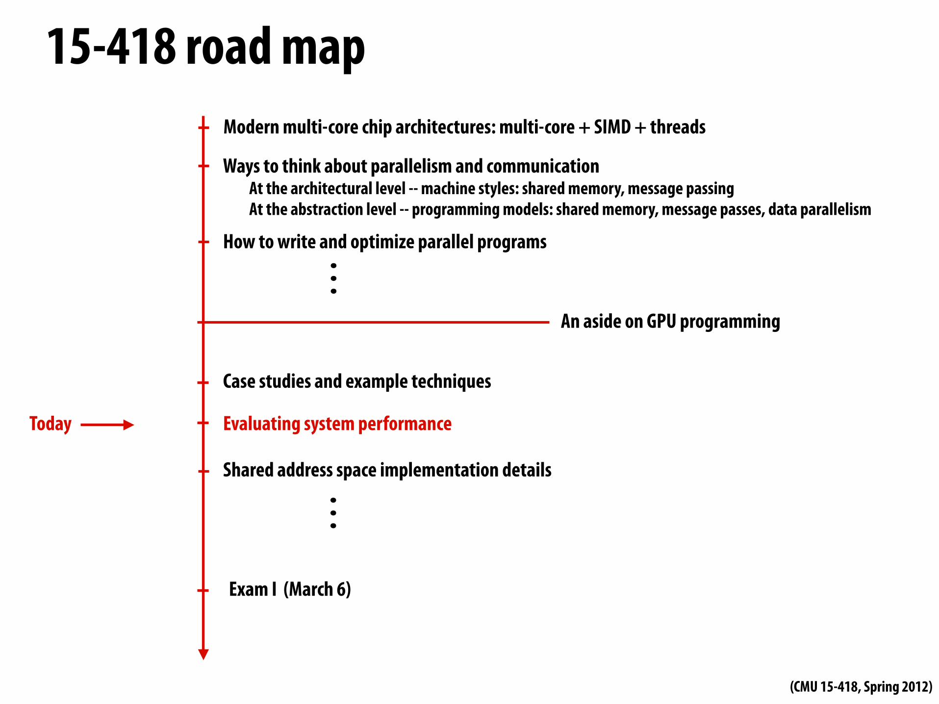
15-418 road mapModern multi-core chip architectures: multi-core + SIMD + threads

Ways to think about parallelism and communicationAt the architectural level -- machine styles: shared memory, message passingAt the abstraction level -- programming models: shared memory, message passes, data parallelism

How to write and optimize parallel programs

An aside on GPU programming

Case studies and example techniques

Evaluating system performance

Shared address space implementation details

. . .

. . .

Exam I (March 6)

Today

(CMU 15-418, Spring 2012)

You are hired by [insert your favorite chip company here].

You walk in on day one, and your boss says“All of our senior architects have decided to take the year off. Your job is to lead the design of our next parallel processor.”

What questions might you ask?

(CMU 15-418, Spring 2012)

Your boss selects the program that matters most to the company“I want you to demonstrate good performance on this application.”

▪ Absolute performance- Often measured as wall clock time- Another example: operations per second

▪ Speedup: performance improvement due to parallelism- Execution time of sequential program / execution time on P processors- Operations per second on P processors / operations per second of sequential program

(CMU 15-418, Spring 2012)

Scaling▪ Should speedup be measured against the parallel program

running on one processor, or the best sequential program?- Example: particle binning problem from last time

(data-parallel algorithm would not be used on a single processor system)

1 320

5 764

9 11108

13 151412

0

12

4

5

3

(CMU 15-418, Spring 2012)

Speedup of ocean application: 258 x 258 grid

Spee

dup

Processors1 32168

Execution on 32 processor SGI Origin 2000

(CMU 15-418, Spring 2012)

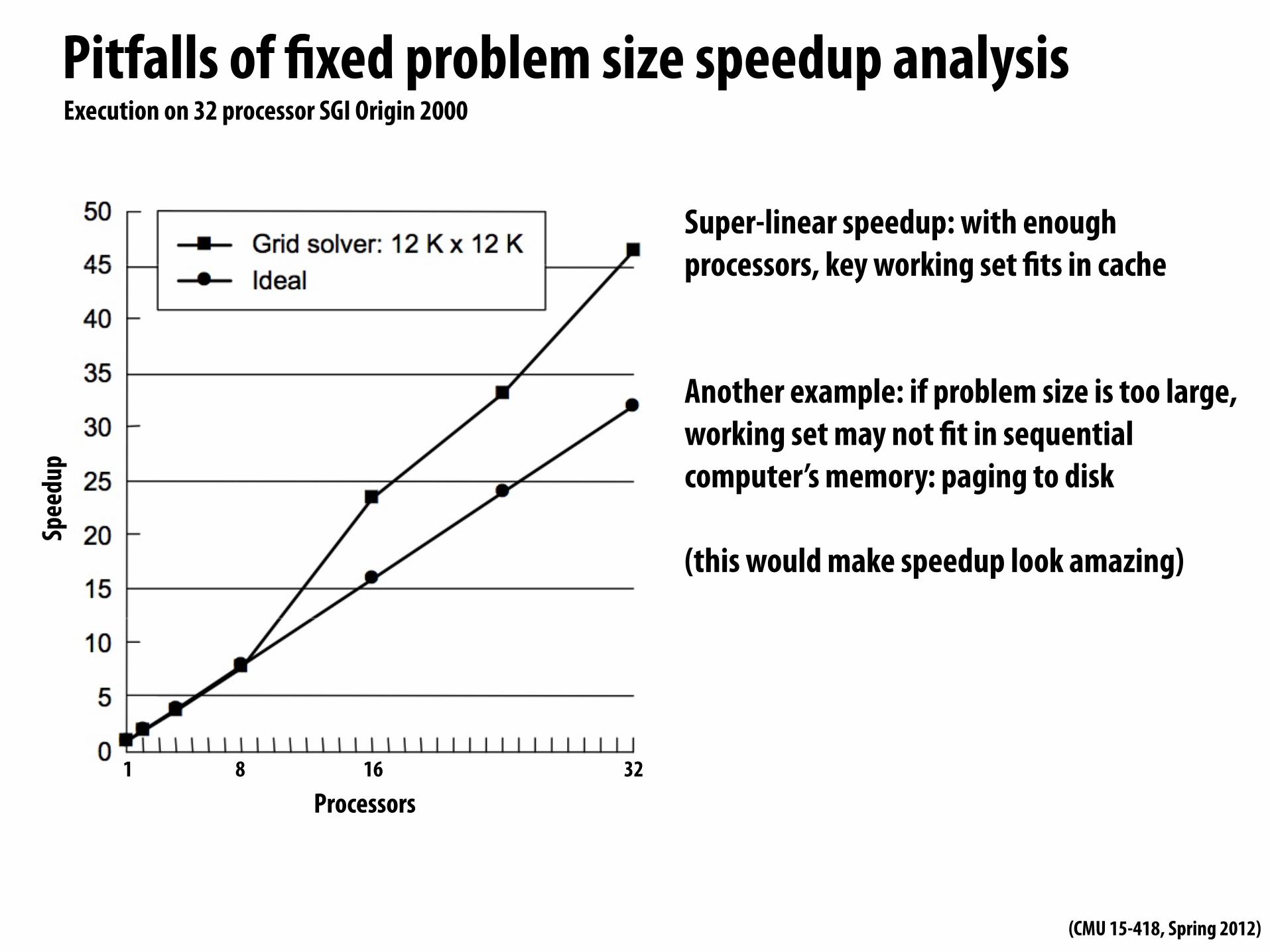
Pitfalls of "xed problem size speedup analysis

Spee

dup

Processors1 32168

Execution on 32 processor SGI Origin 2000

Ideal

258 x 258 grid on 32 processors: ~ 310 grid cells per processor 1K x 1K grid on 32 processors: ~ 32K grid cells per processor

no bene"t(slight slowdown)

Problem is just too small for the machine

(CMU 15-418, Spring 2012)

Pitfalls of "xed problem size speedup analysisSp

eedu

p

Processors1 32168

Execution on 32 processor SGI Origin 2000

Super-linear speedup: with enough processors, key working set "ts in cache

Another example: if problem size is too large, working set may not "t in sequential computer’s memory: paging to disk

(this would make speedup look amazing)

(CMU 15-418, Spring 2012)

Understanding scaling: size matters▪ Application and system scaling parameters have complex interactions

- Impact load balance, overhead, communication-to-computation ratios (inherent and artifactual), locality of data access

- Effects often dramatic, sometimes small, application dependent

▪ Evaluating a machine with a "xed problem size can be problematic- Too small a problem:

- Parallelism overheads dominate parallelism bene"ts for large machines- May even result in slowdowns- May be appropriate for small machines, but inappropriate for large ones

(does not re#ect real usage!)

- Too large a problem: (chosen to be appropriate for large machine)- May not “"t” in small machine

(thrashing to disk, key working set exceeds cache capacity, can’t run at all)- When problem “"ts” in a larger machine, super-linear speedups can occur

- Often desirable to scale problem size as machine sizes grow(not just compute the same size of problems faster)

(CMU 15-418, Spring 2012)

Scaling machines

▪ Ability to scale machines is important

▪ Scaling up: how does its performance scale with increasing processing count?- Will design scale to the high end?

▪ Scaling down: how does its performance scale with decreasing processor count?- Will design scale to the low end?

▪ Parallel architectures designed to work in a range of contexts- Same architecture used, but sized differently for low end, medium scale, high

end systems- GPUs are a great example

“Does it scale?”

(CMU 15-418, Spring 2012)

Questions when scaling a problem▪ Under what constraints should the problem be scaled?

- Fixed data set size, memory usage per processor, execution time, etc.?- Work may no longer be quantity that is "xed

▪ How should be the problem be scaled?

▪ Problem size: de"ned by vector of input parameters- Determines amount of work done- Ocean example: PROBLEM = (n, ε, Δt, T)

grid size

convergence threshold

time step

total time to simulate

(CMU 15-418, Spring 2012)

Scaling constraints

▪ User-oriented scaling properties: speci"c to application domain-Particles per processor- Transactions per processor

▪ Resource-oriented scaling properties1. Problem constrained scaling (PC)2. Memory constrained scaling (MC)3. Time constrained scaling (TC)

User-oriented properties often more intuitive, but resource-oriented properties are more general, apply across domains.

(so we’ll talk about them here)

(CMU 15-418, Spring 2012)

▪ Focus: use a parallel computer to solve the same problem faster

▪ Recall pitfalls from earlier in lecture (small problems not realistic workloads for large machines, big problems don’t "t on small machines)

▪ Examples:- Almost everything we’ve considered parallelizing in class so far- All the problems in assignment 1

Problem-constrained scaling

Speedup = time 1 processor time P processors

(CMU 15-418, Spring 2012)

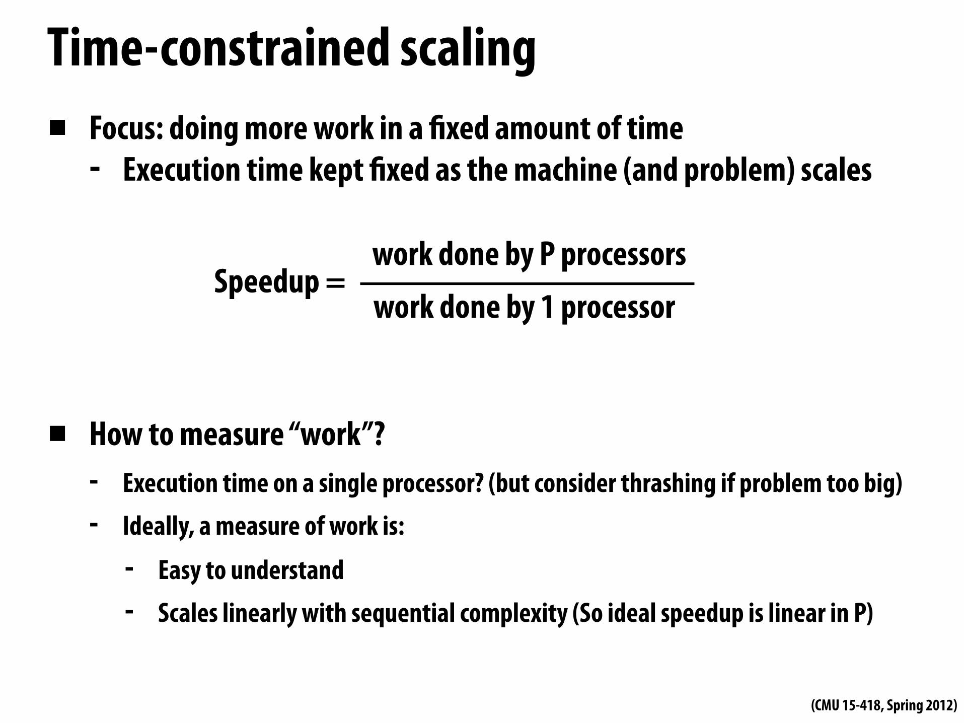
Time-constrained scaling▪ Focus: doing more work in a "xed amount of time

- Execution time kept "xed as the machine (and problem) scales

▪ How to measure “work”?- Execution time on a single processor? (but consider thrashing if problem too big)- Ideally, a measure of work is:

- Easy to understand- Scales linearly with sequential complexity (So ideal speedup is linear in P)

Speedup = work done by P processors work done by 1 processor

(CMU 15-418, Spring 2012)

Time-constrained scaling examples▪ Assignment 2

- Want real-time frame rate: ~ 30 fps- Faster GPU → use capability for more complex scene, not more fps

▪ Computational "nance- Run most sophisticated model possible in: 1 hour, overnight, etc.

▪ Modern web sites- Want to generate complex page, respond to user in X milliseconds.

(CMU 15-418, Spring 2012)

Memory-constrained scaling▪ Focus: run the largest problem possible without over#owing main

memory **▪ Memory per processor held "xed▪ Neither work or execution time are held constant

▪ Note: scaling problem size can make runtimes very large- Consider O(N3) matrix multiplication on O(N2) matrices

** Assumptions: (1) memory resources scale with processor count (2) spilling to disk is infeasible behavior (too slow)

Speedup =

work per unit time on P processors work per unit time on 1 processor

work(P processors) x time(1 processor) time(P processors) x work(1 processor)

=

(CMU 15-418, Spring 2012)

Scaling examples at PIXAR▪ Rendering a movie “shot” (a sequence of frames)

- Minimizing time to completion (problem constrained)- Assign each frame to a different machine in the cluster

▪ Artists working to design lighting for a scene- Provide interactive frame rate in application (time constrained)- Buy large multi-core workstations (more performance = higher "delity

representation shown to artist)

▪ Physical simulation: e.g., #uids- Parallelize simulation across multiple machines to "t simulation in memory

(memory constrained)

▪ Final render- Scene complexity bounded by memory available on farm machines- One barrier to exploiting additional parallelism is that footprint often increases

with number of processors (memory constrained)

(CMU 15-418, Spring 2012)

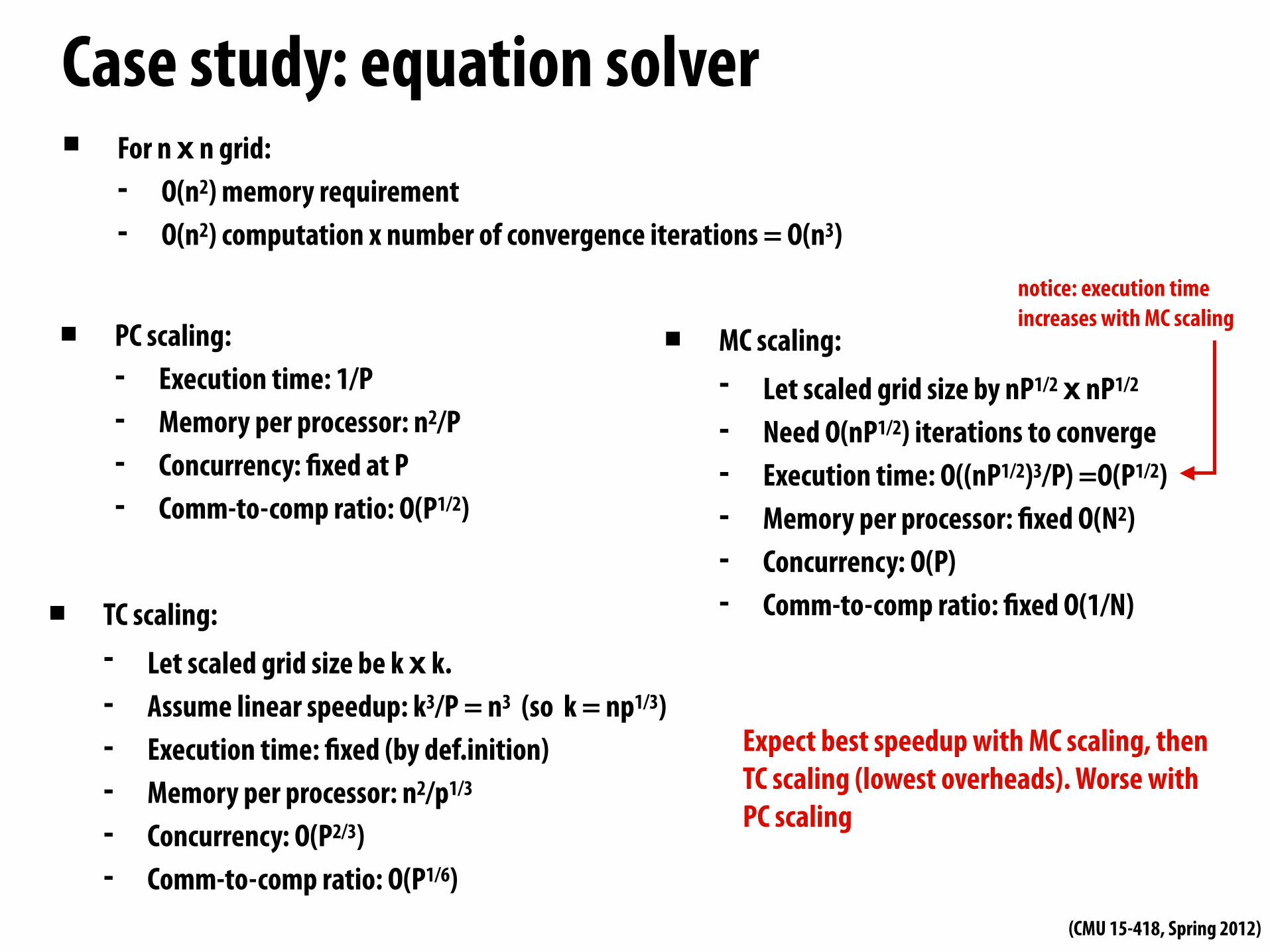
Case study: equation solver▪ For n x n grid:

- O(n2) memory requirement- O(n2) computation x number of convergence iterations = O(n3)

▪ PC scaling:- Execution time: 1/P - Memory per processor: n2/P- Concurrency: "xed at P- Comm-to-comp ratio: O(P1/2)

▪ TC scaling:- Let scaled grid size be k x k.- Assume linear speedup: k3/P = n3 (so k = np1/3)- Execution time: "xed (by def.inition) - Memory per processor: n2/p1/3

- Concurrency: O(P2/3)- Comm-to-comp ratio: O(P1/6)

▪ MC scaling:- Let scaled grid size by nP1/2 x nP1/2 - Need O(nP1/2) iterations to converge- Execution time: O((nP1/2)3/P) =O(P1/2)- Memory per processor: "xed O(N2)- Concurrency: O(P)- Comm-to-comp ratio: "xed O(1/N)

notice: execution time increases with MC scaling

Expect best speedup with MC scaling, then TC scaling (lowest overheads). Worse with PC scaling

(CMU 15-418, Spring 2012)

Word of caution about problem scaling

▪ Problem size in the pervious examples was a single parameter n

▪ In practice, problem size is a combination of parameters- Example from Ocean: = (n, ε, Δt, T)

▪ Problem parameters are often related (not independent)- Example from Barnes-Hut: increasing star count n changes required

simulation time step and force calculation accuracy parameter ϴ

▪ Must be cognizant of these relationships when scaling problem in TC or MC scaling

(CMU 15-418, Spring 2012)

Scaling summary

▪ Performance improvement due to parallelism is measured by speedup

▪ But speedup metrics take different forms for different scaling models- Which model matters most is application/context speci"c

▪ In addition to assignment and orchestration, behavior of a parallel program depends signi"cantly on problem and machine scaling properties- When analyzing performance, be sure to analyze realistic regimes of

operation (both realistic sizes and realistic problem size parameters)- Requires application knowledge

(CMU 15-418, Spring 2012)

You have an idea for how to design a parallel machine to meet the needs of your boss.

How are you going to test this idea?

Back to our example of your hypothetical future job...

(CMU 15-418, Spring 2012)

Evaluating an architectural idea: simulation

▪ Architects evaluate architectural decisions quantitatively using simulation- Run with new feature, run without feature, compare simulated performance- Simulate against a wide collection of benchmarks

▪ Design detailed simulator to test new architectural feature- Very expensive to simulate a parallel machine in full detail- Often cannot simulate full machine con"gurations or realistic problem sizes

(must scale down signi"cantly!)- Architects need to be con"dent scaled down simulated results predict reality

(otherwise, why do the evaluation at all?)

(CMU 15-418, Spring 2012)

Execution-driven simulator

▪ Executes simulated program in software- Simulated processors generate memory references, which are processed by the

simulated memory hierarchy

▪ Performance of simulator typically inversely proportional to level of simulated detail

Memory Reference Generator Memory Hierarchy Simulator

(CMU 15-418, Spring 2012)

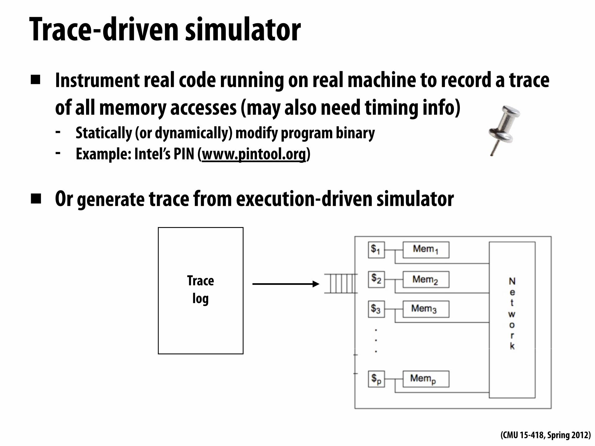
Trace-driven simulator▪ Instrument real code running on real machine to record a trace

of all memory accesses (may also need timing info)- Statically (or dynamically) modify program binary- Example: Intel’s PIN (www.pintool.org)

▪ Or generate trace from execution-driven simulator

Tracelog

(CMU 15-418, Spring 2012)

Scaling down challenges▪ Preserve distribution of time spent in program phases

- e.g., Ray-trace and Barnes-Hut: both have tree build and tree traverse phases

▪ Preserve important behavioral characteristics- communication-to-computation ratio, load balance, locality, working set sizes

▪ Preserve contention and communication patterns- tough, contention is a function of timing and ratios

▪ Preserve scaling relationships between problem parameters- e.g., Barnes-Hut: scaling up particle count requires scaling down time step for

physics reasons

(CMU 15-418, Spring 2012)

Example: scaling down Barnes-Hut▪ Problem size = (n, ϴ, Δt, T)

grid sizeaccuracy threshold

time step

total time to simulate

▪ Easiest parameter to scale down is likely T (just simulate less time)- Independent of the other parameters- If simulation characteristics don’t vary much over time- Or select a few representative T (beginning of sim, end of sim)

(CMU 15-418, Spring 2012)

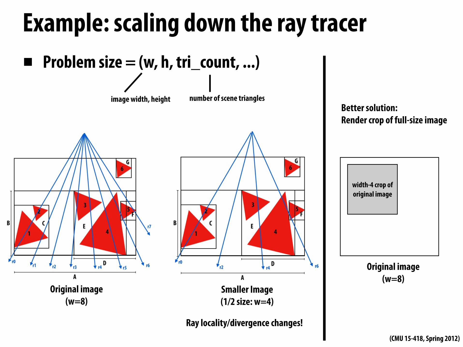
Example: scaling down the ray tracer▪ Problem size = (w, h, tri_count, ...)

image width, height number of scene triangles

Original image(w=8)

Smaller Image(1/2 size: w=4)

Original image(w=8)

width-4 crop of original image

Better solution:Render crop of full-size image

Ray locality/divergence changes!

(CMU 15-418, Spring 2012)

Note: issues of scaling down also apply to debugging/tuning software running on existing machines

Common example:May want to log behavior of code for debugging. Instrumentation slows down code signi"cantly, logs get untenable in size quickly.

(CMU 15-418, Spring 2012)

Architectural simulation state space▪ Another evaluation challenge: dealing

with large parameter space of machines- Num processors, cache sizes, cache line sizes,

memory bandwidths, etc.

▪ Decide what parameters are relevant and prune space!

Cache size

Miss

rate

unrealistic operating point: cache too large

unrealistic operating point: miss rate too high

= con"guration to simulate

Paredo Curve(plots energy/perf trade-off)

Performance Density (ops/nS/mm2)

Ener

gy Pe

r Ope

ratio

n (nJ

/op)

(CMU 15-418, Spring 2012)

Today’s summary: BE CAREFUL!

It can be very tricky to evaluate parallel software and machines.

It can be easy to obtain misleading results.

It is helpful to precisely state your application goals. Then determine if evaluation approach is consistent with those goals.

(CMU 15-418, Spring 2012)

Some tricks for evaluating the performance of software

(CMU 15-418, Spring 2012)

Determine if performance is limited by computation, memory bandwidth (or latency), or synchronization **

Add mathDoes runtime increase linearly with additional computation?

Change all array accesses to A[0]How much faster does your code get?(this is an upper bound on bene"t of exploiting locality)

Remove all atomic operations or locksHow much faster does your code get?(this is an upper bound on bene"t of reducing sync overhead)

Remove almost all math, load same dataHow much does runtime decrease? If not much, suspect bandwidth limits

** Often all of these effects are in play because compute, memory access, and synchronization are not perfectly overlapped. As a result, overall performance is not-dominated by exactly one type of behavior