CMPE 150 – Winter 2009

Lecture 11

February 12, 2009

P.E. Mantey

CMPE 150 -- Introduction to Computer Networks

Instructor: Patrick Mantey mantey@soe.ucsc.edu http://www.soe.ucsc.edu/~mantey/

Office: Engr. 2 Room 595J Office hours: Tues 3-5 PM, Mon 5-6 PM* TA: Anselm Kia akia@soe.ucsc.edu Web site: http://www.soe.ucsc.edu/classes/cmpe150/Winter09/

Text: Tannenbaum: Computer Networks (4th edition – available in bookstore, etc. )

Syllabus

Today’s Agenda Routing (continued)

Distance Vector Protocol Link State Routing

Network Layer Hierarchical Routing Broadcast Routing Spanning Tree Routing Congestion Control Quality of Service Internetworking

Reading Assignment

Today: Chapter 5, sections 5.2.4-8 (continued), 5.3, 5.4.1-5.4.3

Tuesday: Tannenbaum, Chapter5, section 5.5, 5.6: Internet Protocol

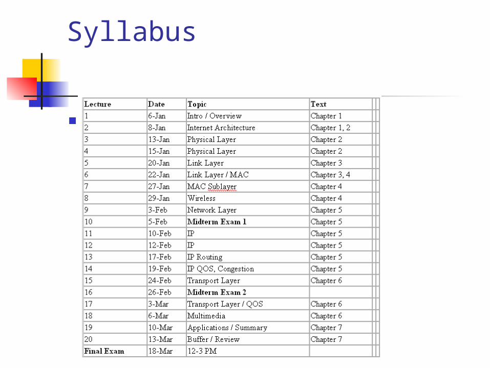
Internet Layering

Level 5 -- Application Layer (rlogin, ftp, SMTP, POP3, IMAP, HTTP..)

Level 4 -- Transport Layer(a.k.a Host-to-Host)(TCP, UDP, ARP, ICMP, etc.)

Level 3 -- Network Layer (a.k.a. Internet) (IP)Level 2 -- (Data) Link Layer / MAC sub-layer

(a.k.a. Network Interface or Network Access Layer)

Level 1 -- Physical Layer

Distance-Vector protocol

Initialize routing table with local linksFlood routing table to all routersDo

Compute local routing table from graphWait for update or link cost change or timerUpdate network graphIf link cost change

Flood updated link to all routers Else if timer expired

Flood routing table to all routersForever

Distance Vector Routing

(a) A subnet. (b) Input from A, I, H, K, and the new routing table for J.

Distance Vector Routing 1 Each router keeps routing table (or routing

vector) giving best known distance to each destination and the corresponding outgoing interface.

Routing tables are updated by exchanging routing information with neighbors.

Implements distributed version of Bellman-Ford

Aka Ford-Fulkerson Timer-based refresh vs neighbor tables

Distance Vector 2

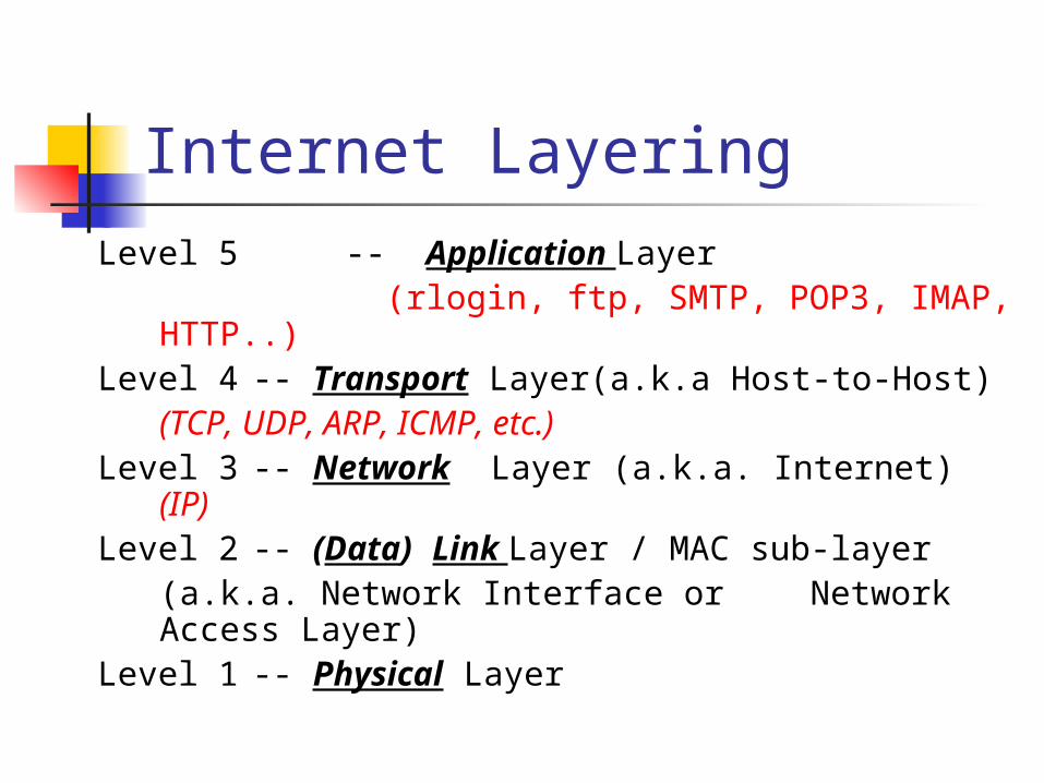
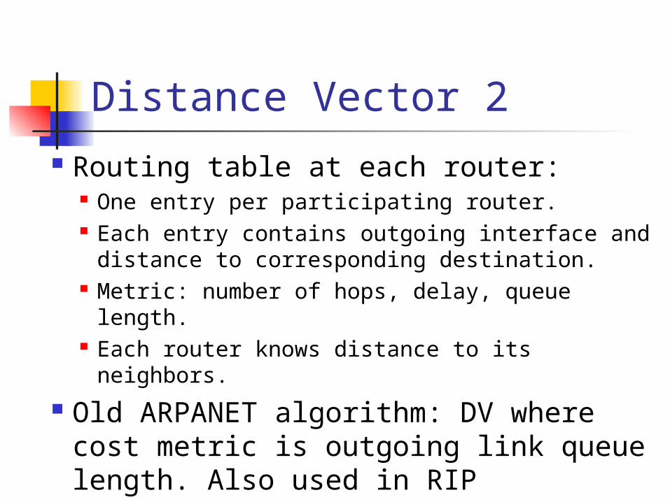
Routing table at each router: One entry per participating router. Each entry contains outgoing interface and

distance to corresponding destination. Metric: number of hops, delay, queue

length. Each router knows distance to its neighbors.

Old ARPANET algorithm: DV where cost metric is outgoing link queue length. Also used in RIP

Routing Updates Every T interval, routers exchange routing

updates. Routing update from router X consists of a

vector with all destinations and the corresponding distance from X to them.

When router Y receives an update from X, it can estimate its distance to router Z through X as Dyz = Dyx + Dxz.

Router Y receives update from all its neighbors; discards its RT and builds a new one.

Distance Vector: Example

1

4

6

2 3

5

1Node Distance Next

2

33

2

19

5

1

2

1 0 -

2 2 2

3 5 3

4 1 45 6 3

6 8 3

T=T0T=T1

3 7 5

2 3 4

0 4 2

3 0 2

2 2 03 1 15 3 3

Node Distance Next

1 0 -

2

3

4 5

6

T=T2

7

Distance Vector: Example

1

4

6

2 3

5

1Node Distance Next

2

33

2

19

5

1

2

1 0 -

2 2 2

3 5 3

4 1 45 6 3

6 8 3

T=T0T=T1

3 7 5

2 3 4

0 4 2

3 0 2

2 2 03 1 15 3 3

Node Distance Next

1 0 -

2 2 2

3 3 4

4 1 45 2 4

6 4 4

T=T2

7

Problems

1. Routing loops.2. Slow convergence.3. Counting to infinity.

Bellman-Ford overview Network represented by graph: G(V,E)

V contains vertices i,j,… E contains edges (i,j), …

Algorithm data structures “s” - source vertex “dij” - cost of the edge (i,j); dij = ∞ if (i,j) E

“Dhi” - cost of the shortest path with h hops from s to

i

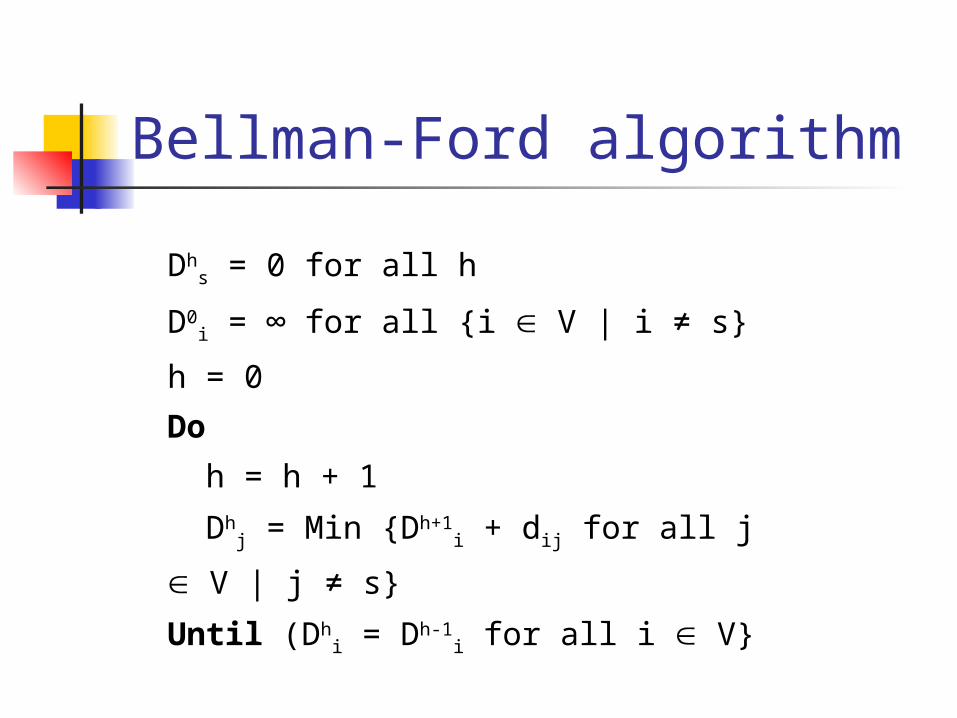
Bellman-Ford algorithm

Dhs = 0 for all h

D0i = ∞ for all {i V | i ≠ s}

h = 0

Do

h = h + 1

Dhj = Min {Dh+1

i + dij for all j V | j ≠

s}

Until (Dhi = Dh-1

i for all i V}

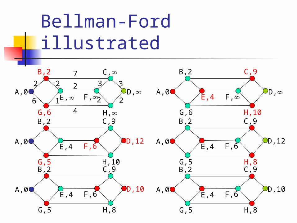
Bellman-Ford illustrated

6

2 2

2

C,

F,E,1A,0

B,2

D,

G,6 H,

73

2

32

4

C,9

F,E,4A,0

B,2

D,

G,6 H,10C,9

F,6E,4A,0

B,2

D,12

G,5 H,10

C,9

F,6E,4A,0

B,2

D,12

G,5 H,8C,9

F,6E,4A,0

B,2

D,10

G,5 H,8

C,9

F,6E,4A,0

B,2

D,10

G,5 H,8

Count-to-Infinity 1

Good news propagates faster.

A B C D E

Initially, A down:A comes up:

infinity11 2 infinity infinity (after 2 exchanges)1 2 3 infinity (after 3 exchanges)1 2 3 4 (after 4 exchanges)

infinityinfinity

infinityinfinity

infinityinfinity (after 1 exchange)

Count-to-Infinity 2

But, bad news propagate slower!

A B C D E

Initially, all up:A goes down:

1 2 3 43 2 3 4 (after 1 exchange)3 4 3 4 (after 2 exchanges)5 4 5 4 (after 3 exchanges)5 6 5 6 (after 4 exchanges)7 6 7 6 (after 5 exchanges)7 8 7 8 (after 6 exchanges)

….infinity

Count-to-Infinity 3

Gradually routers work their way up to infinity.

Number of exchanges depends on how large is infinity.

To reduce number of exchanges, if metric is number of hops, infinity=maximum path+1.

Solution Routing loops:

Path vector: record actual path used in the DV. Previous hop tracing: records preceding router.

Count-to-infinity: Split horizon: router doesn’t report true route to next hop of

the previous route Poison reverse: router “infinity” to next hop of previous route Split horizon with poison reverse prevent loops involving two

routers Triggered updates: if the metric for a route is changed, send

an update immediately In the absence of other updates, this solves the problem… in

reality, other updates will “keep hope alive” RFC1058 is a good reference for these issues

Split Horizon

Tries to make bad news spread faster. A node reports infinity as distance to

node X on link packets to X are sent on. Example, in the first exchange, C tells D

its distance to A but tells B its distance to A is infinity. So B discovers its link to A is down

and C’s distance to A is infinity; so it sets its distance to A to infinity.

Link-State protocol

Initialize network graph with local linksFlood local links to all routersDo

Compute local routing table from graphWait for update or link cost changeUpdate network graphIf link cost change

Flood updated link to all routersForever

Link State Routing 1

Link State routing used in the ARPAnet starting in 1979

Used by the Internet’s OSPF(Open Shortest Path First)

Link State Routing 2

Link state routing is based on: Discover your neighbors and measure

the communication cost to them. Send updates about your neighbors to all

other routers. Compute shortest path to every other

router.

Finding Neighbors

When router is booted, its first task is to find who its neighbors are.

Special single-hop “hello” packets. Cost metric:

Number of hops: in this case, always 1. Delay: “echo” packets and measure RTT/2. Load?

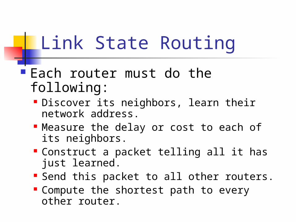
Link State Routing Each router must do the

following: Discover its neighbors, learn their

network address. Measure the delay or cost to each of its

neighbors. Construct a packet telling all it has just

learned. Send this packet to all other routers. Compute the shortest path to every other

router.

Generating Link State Updates

Link state packets (LSP). Sender identity. Sequence number. TTL. List of (neighbor, cost).

When to send updates? Proactive: periodic updates; how often? Reactive: whenever some significant event is

detected, e.g., link goes down. Where to send them? Everywhere: flood.

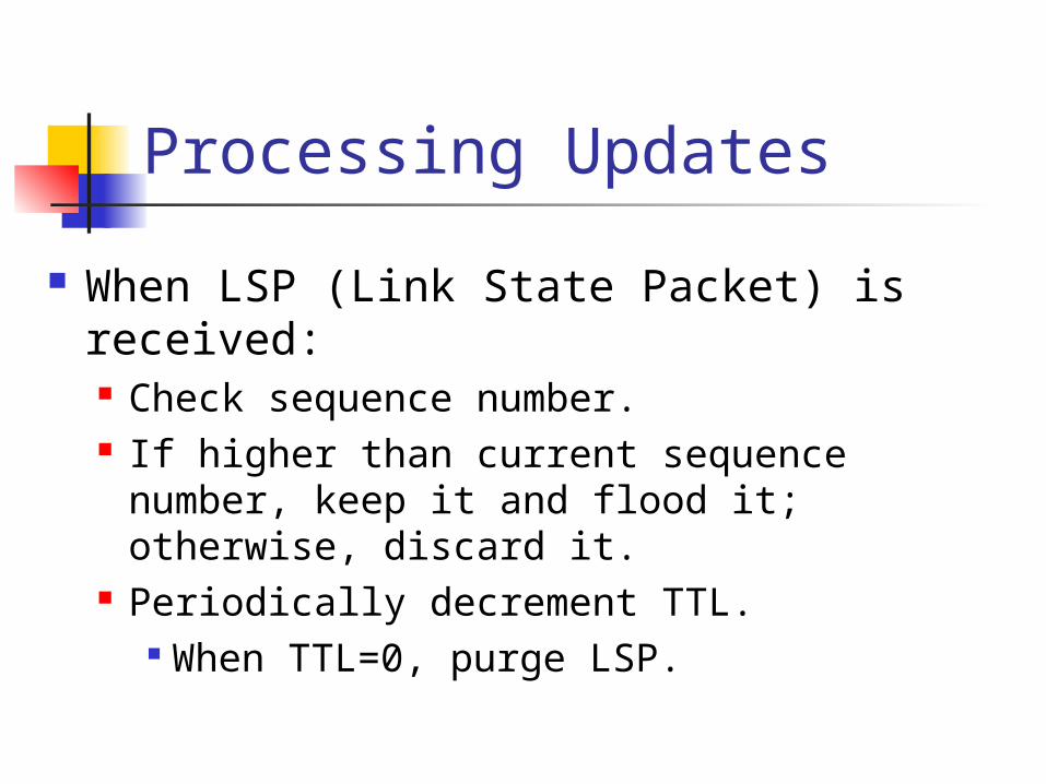
Processing Updates

When LSP (Link State Packet) is received: Check sequence number. If higher than current sequence number,

keep it and flood it; otherwise, discard it. Periodically decrement TTL.

When TTL=0, purge LSP.

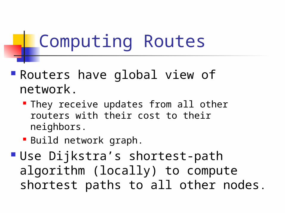
Computing Routes

Routers have global view of network. They receive updates from all other routers

with their cost to their neighbors. Build network graph.

Use Dijkstra’s shortest-path algorithm (locally) to compute shortest paths to all other nodes.

Learning about the Neighbors

(a) Nine routers and a LAN. (b) A graph model of (a).

Measuring Line Cost

A subnet in which the East and West parts are connected by two lines.

Building Link State Packets

(a) A subnet. (b) The link state packets for this subnet.

Distributing the Link State Packets

The packet buffer for router B in the previous slide (Fig. 5-13).

DV versus LS

DV: Tell neighbors what you know about everybody. Choose best route given neighbor’s routing tables. Distributed computation. Topology information distributed only where

needed LS:

Tell everyone what you know about neighbors. Every node has global view. Compute their own routes. Topology information distributed to everyone

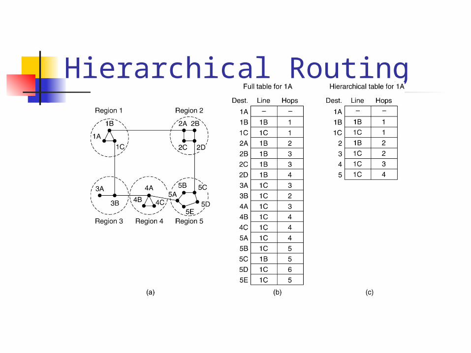
Hierarchical Routing For scalability:

As network grows, so does RT size, routing update generation, processing, and propagation overhead, and route computation time and resources.

Divide network into routing regions. Routers within region know how to route packets

to all destinations within region. But don’t know how to route within other

regions. “Border” routers: route within regions.

Hierarchical Routing Example

1B

1A 1C

2A 2B

2C2D

3A 3B

4A

4B 4C

5E 5D

5C

5B

5A

Dest. Next Hops1A - -1B 1B 11C 1C 12A 1B 22B 1B 32C 1B 32D 1B 43A 1C 33B 1C 24A 1C 34B 1C 44C 1C 45A 1C 45B 1C 55C 1B 55D 1C 65E 1C 5

1A

Hierarchical Routing Example

1B

1A 1C

2A 2B

2C2D

3A 3B

4A

4B 4C

5E 5D

5C

5B

5A

Dest. Next Hops1A - -1B 1B 11C 1C 12 1B 23 1C 24 1C 35 1C 4

A

Hierarchical Routing

Hierarchical Routing

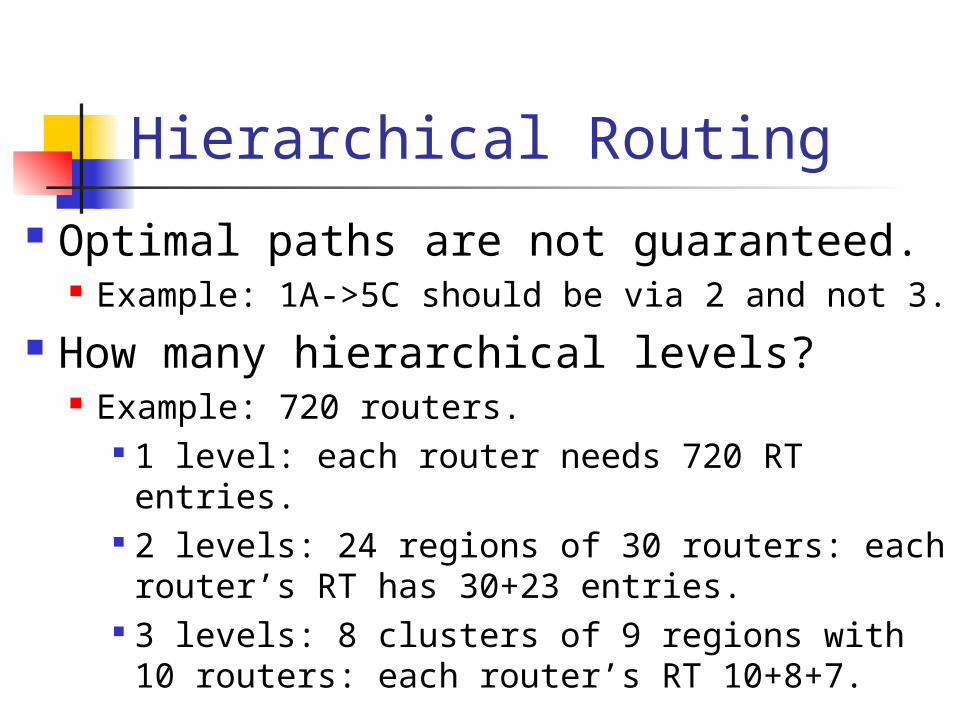
Optimal paths are not guaranteed. Example: 1A->5C should be via 2 and not 3.

How many hierarchical levels? Example: 720 routers.

1 level: each router needs 720 RT entries. 2 levels: 24 regions of 30 routers: each

router’s RT has 30+23 entries. 3 levels: 8 clusters of 9 regions with 10

routers: each router’s RT 10+8+7.

Many-to-Many Routing

Support many-to-many communication.

Example applications: multi-point data distribution, multi-party teleconferencing.

Many-to-Many Routing

Broadcasting Flooding Multidestination routing Spanning tree Reverse path forwarding

Broadcasting

Simplistic approach: send separate packet to each destination. Simple but expensive. Source needs to know about all

destinations.

Flooding: May generate too many duplicates

(depending on node connectivity).

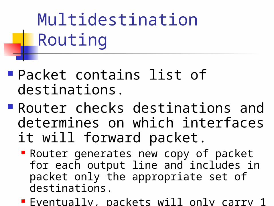
Multidestination Routing

Packet contains list of destinations. Router checks destinations and

determines on which interfaces it will forward packet. Router generates new copy of packet for

each output line and includes in packet only the appropriate set of destinations.

Eventually, packets will only carry 1 destination.

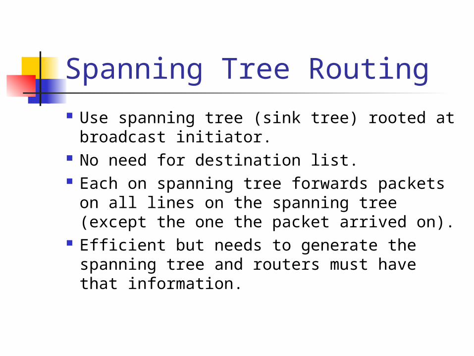
Spanning Tree Routing Use spanning tree (sink tree) rooted at

broadcast initiator. No need for destination list. Each on spanning tree forwards packets on

all lines on the spanning tree (except the one the packet arrived on).

Efficient but needs to generate the spanning tree and routers must have that information.

Reverse Path Forwarding

Routers don’t have to know spanning tree.

Router checks whether broadcast packet arrived on interface used to send packets to source of broadcast. If so, it’s likely that it followed best route and

thus not a duplicate; router forwards packet on all lines.

If not, packet discarded as likely duplicate.

Broadcast Routing

Reverse path forwarding. (a) A subnet. (b) a Sink tree. (c) The tree built by reverse path forwarding.

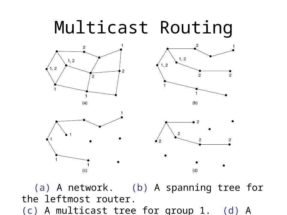
Multicast Routing

(a) A network. (b) A spanning tree for the leftmost router. (c) A multicast tree for group 1. (d) A multicast tree for group 2.

Multicasting• Special form of broadcasting:

– Instead of sending messages to all nodes, send messages to a group of nodes.

• Multicast group management:– Creating, deleting, joining, leaving group.– Group management protocols communicate group

membership to appropriate routers.

Multicast Routing

• Each router computes spanning tree covering all other participating routers.– Tree is pruned by removing that do not

contain any group members.

1,2

1

1,22

21

1

21,2

1

1,22

2

1

1

2

1

1

1

1

12 2

2

2 2

Shared Tree Multicasting

• Source-rooted tree approaches don’t scale well!– 1 tree per source, per group!– Routers must keep state for m*n trees, where m is number of sources in a group and n is number of groups.

• Core-based trees: single tree per group.– Host unicast message to core, where

message is multicast along shared tree.– Routes may not be optimal for all sources.– State/storage savings in routers.

Other Simulations / Animations

http://cisr.nps.edu/downloads/wecs7_ch9.pdf

Congestion Control

Ideal network behavior:

Packetsdelivered

Packetssent

Maximum capacity

Congestion

When too much traffic is offered, congestion sets in and performance degrades sharply.

Congestion and Policies

• Policies that affect congestion.

5-26

General Principles of Congestion Control

1. Monitor the system.detect when and where congestion occurs.

2. Pass information to where action can be taken.

3. Adjust system operation to correct the problem.

Network Congestion What is network congestion?

Too many packets in the network. Router queues are always full.

Routers start dropping packets. Congestion can fuel itself.

Packet drops lead to retransmissions. More traffic!

May result in congestion collapse! Close to 0 throughput!

Infinite-Buffer Routers

Intuition says add more memory to routers and that’ll avoid congestion. Nagle (1987) showed that infinite buffers

actually make congestion worse. More packets enqueued for long time; they

time out and are retransmitted; but still transmitted by router.

Therefore, more traffic.

Causes of Congestion Mismatch in capacity among

different parts of the system. Mismatch in link speeds. Mismatch in router processing capability.

Table lookup and update. Queue management.

Congestion in one point of network tends to propagate backwards toward sender.

R

Congestion versus Flow Control

Congestion control tries to ensure the network is able to carry offered traffic. Involves hosts and intermediate routers.

Flow control ensures that the communication end-points are able to keep up with one another. Involves only the end-points.

Congestion and Flow Control

Often mixed because tend to use same feedback mechanisms.

Example: “slow down” message received at host may be caused by receiver not being able to keep up with sender host or by network not being able to handle additional traffic.

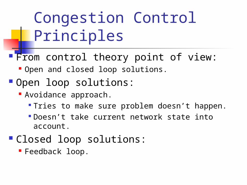
Congestion Control Principles

From control theory point of view: Open and closed loop solutions.

Open loop solutions: Avoidance approach.

Tries to make sure problem doesn’t happen. Doesn’t take current network state into

account.

Closed loop solutions: Feedback loop.

Closed Loop Solutions 3 components:

Monitoring. Feedback generation. Operation adjustment.

Monitoring metrics: Packet loss. Average queue length. Number of retransmitted packets. Average packet delay.

Feedback Send information about the

problem once it’s detected. Router that detects problem sends

packet to traffic source(s). Special-purpose bit in every packet that

router sets when it detects congestion above certain level to warn neighbors.

Special probe messages to detect congested areas so they can be avoided.

Stability: avoid oscillations.

Congestion Control Taxonomy

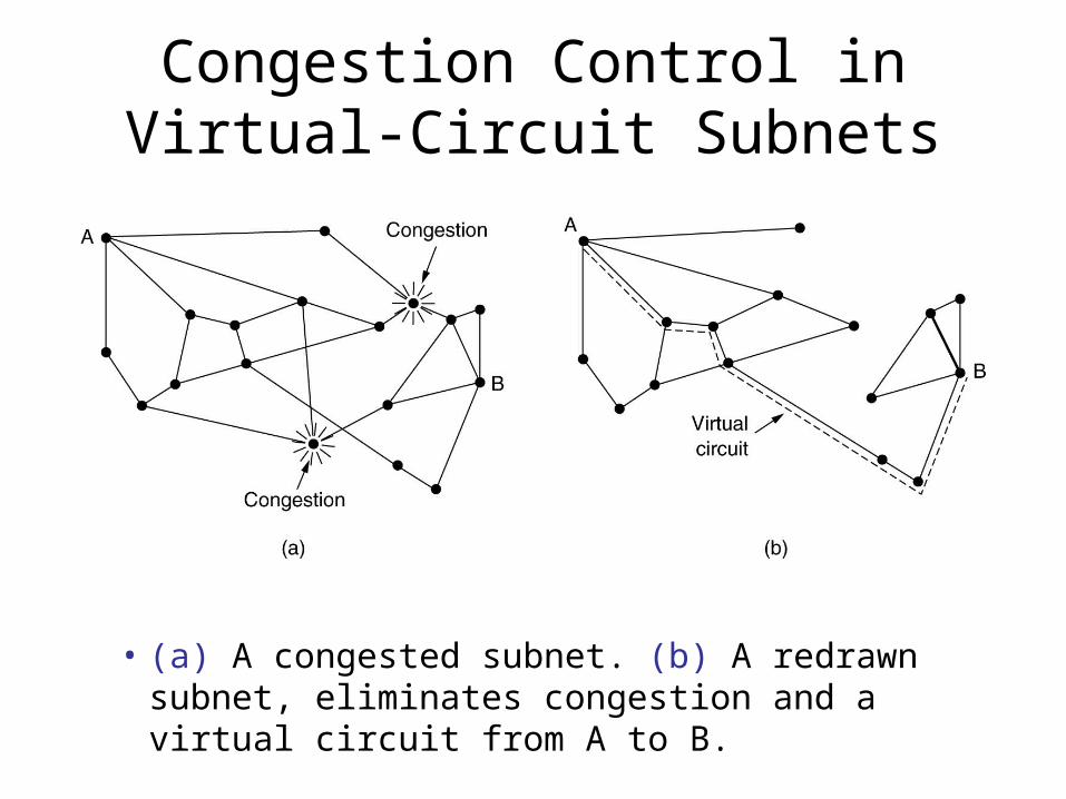
Congestion Control in Virtual-Circuit Subnets

• (a) A congested subnet. (b) A redrawn subnet, eliminates congestion and a virtual circuit from A to B.

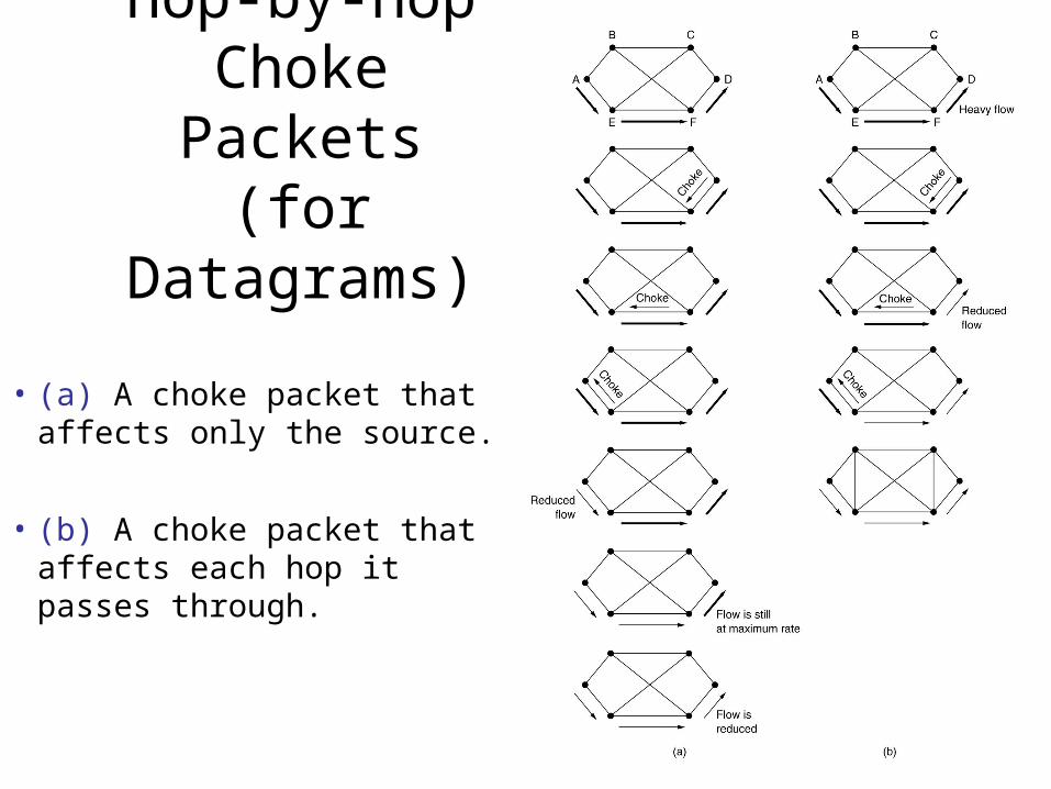
Hop-by-Hop Choke Packets(for Datagrams)

• (a) A choke packet that affects only the source.

• (b) A choke packet that affects each hop it passes through.

Jitter Control

(a)High jitter. (b) Low jitter. Router sends packets furthest behind

schedule

Quality of Service

Requirements Techniques for Achieving Good

Quality of Service Integrated Services Differentiated Services Label Switching and MPLS

Quality of Service Requirements

5-30

Buffering

Smoothing the output stream by buffering packets.

Open Loop Approaches Traffic Shaping

Avoid traffic burstiness by forcing packets to be transmitted at more predictable rate.

Used in ATM networks. Regulates average transmission rate. In contrast to sliding window protocols which

regulate amount of data in transit. Service agreement between user and carrier.

Important to real-time traffic such as audio, video.

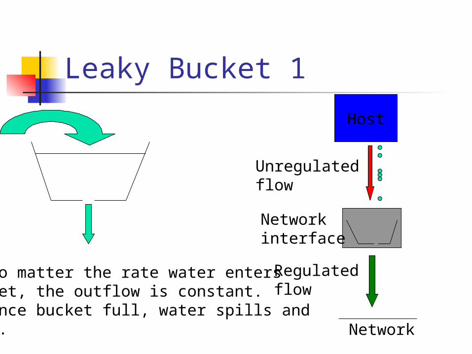
Leaky Bucket 1

1. No matter the rate water entersbucket, the outflow is constant.2. Once bucket full, water spills and lost.

Host

Network

Unregulatedflow

Regulated flow

Networkinterface

Leaky Bucket 2 Equivalent to a single-server queuing system with constant service time. Same size packets (e.g., ATM cells): use packets as unit. Variable-sized packets: use numbr of bytes per clock tick.

The Token Bucket Algorithm

• (a) Before. (b) After.

5-34

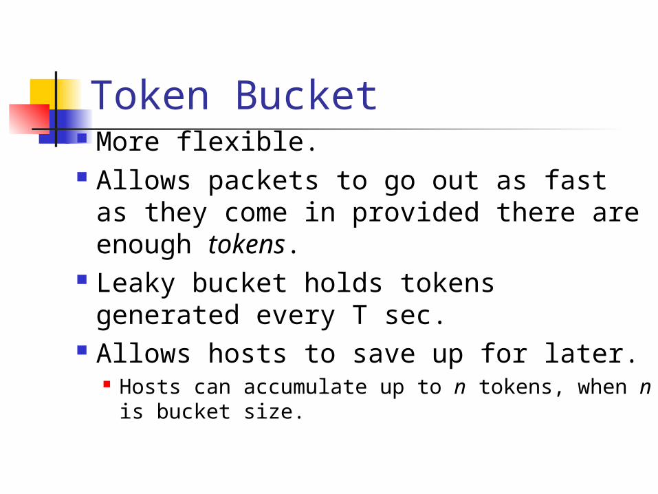
Token Bucket More flexible. Allows packets to go out as fast as

they come in provided there are enough tokens.

Leaky bucket holds tokens generated every T sec.

Allows hosts to save up for later. Hosts can accumulate up to n tokens, when n

is bucket size.

Leaky and Token Bucket

Token bucket throws away tokens but never packets.

Can be used between host and network and between routers.

Token bucket can still produce bursts. Insert leaky bucket after token bucket.

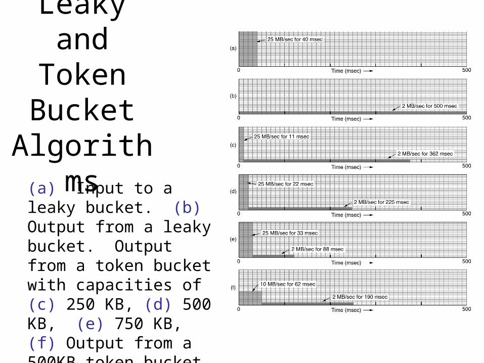
Leaky and Token Bucket

Algorithms(a) Input to a leaky bucket. (b) Output from a leaky bucket. Output from a token bucket with capacities of (c) 250 KB, (d) 500 KB, (e) 750 KB, (f) Output from a 500KB token bucket feeding a 10-MB/sec leaky bucket.

Flow Specifications Way for user/application to specify traffic patterns

and desired quality of service. Before connection established or data is sent,

source provides flow spec to network. Network can accept, reject, or counter-offer.

Example: flow spec language by Partridge (1992). Traffic spec: maximum packet size, maximum

transmission rate. Service desired: maximum acceptable loss rate,

maximum delay and delay variation.

Admission Control

An example of flow specification.

5-34

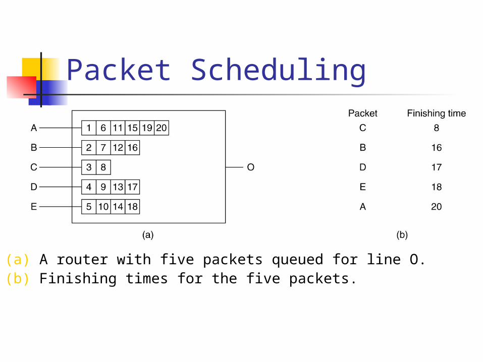
Packet Scheduling

(a) A router with five packets queued for line O.(b) Finishing times for the five packets.

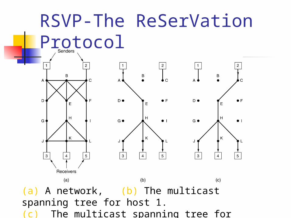
RSVP-The ReSerVation Protocol

(a) A network, (b) The multicast spanning tree for host 1. (c) The multicast spanning tree for host 2.

RSVP-The ReSerVation Protocol (2)

(a) Host 3 requests a channel to host 1. (b) Host 3 then requests a second channel, to host 2. (c) Host 5 requests a channel to host 1.

Expedited Forwarding

Expedited packets experience a traffic-free network.

Assured Forwarding

A possible implementation of the data flow for assured forwarding.

Label Switching and MPLS

Transmitting a TCP segment using IP, MPLS, and PPP.

Internetworking

How Networks Differ How Networks Can Be Connected Concatenated Virtual Circuits Connectionless Internetworking Tunneling Internetwork Routing Fragmentation

Connecting Networks

• A collection of interconnected networks.

How Networks Differ

Some of the many ways networks can differ.

5-43

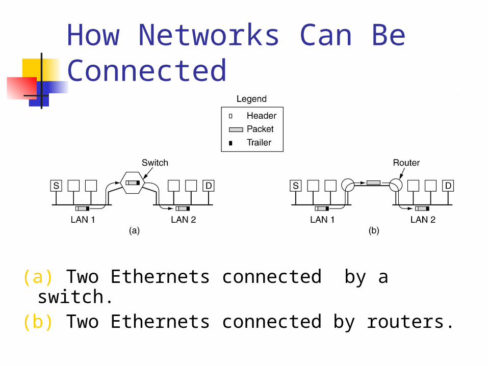
How Networks Can Be Connected

(a) Two Ethernets connected by a switch.

(b) Two Ethernets connected by routers.

Concatenated Virtual Circuits

Internetworking using concatenated virtual circuits.

Connectionless Internetworking

A connectionless internet.

Tunneling

Tunneling a packet from Paris to London.

Tunneling (2)

Tunneling a car from France to England.

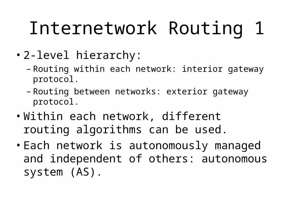
Internetwork Routing 1

• 2-level hierarchy:– Routing within each network: interior gateway protocol.– Routing between networks: exterior gateway protocol.

• Within each network, different routing algorithms can be used.

• Each network is autonomously managed and independent of others: autonomous system (AS).

Internetwork Routing 2• Typically, packet starts in its LAN.

Gateway receives it (broadcast on LAN to “unknown” destination).

• Gateway sends packet to gateway on the destination network using its routing table. If it can use the packet’s native protocol, sends packet directly. Otherwise, tunnels it.

Internetwork Routing

(a) An internetwork. (b) A graph of the internetwork.

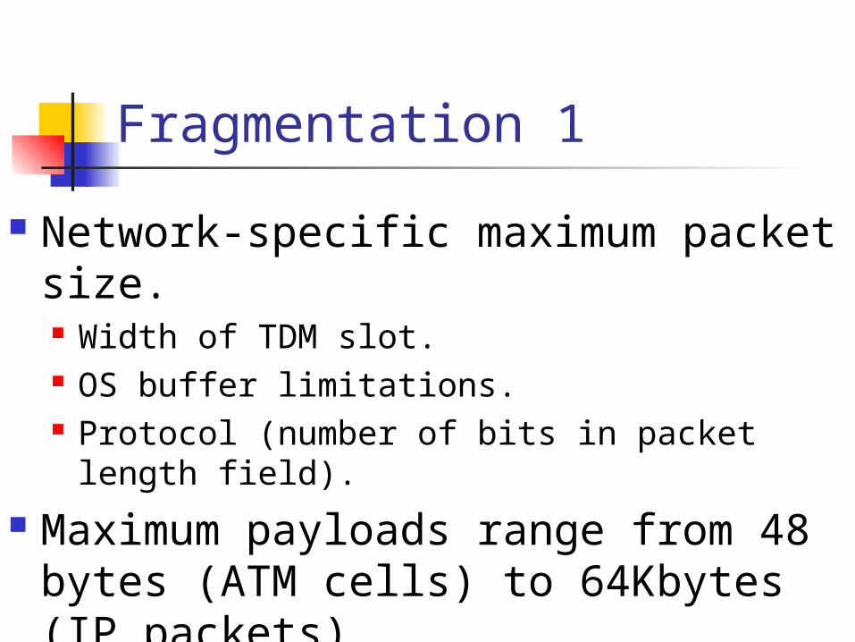
Fragmentation 1

Network-specific maximum packet size. Width of TDM slot. OS buffer limitations. Protocol (number of bits in packet length

field).

Maximum payloads range from 48 bytes (ATM cells) to 64Kbytes (IP packets).

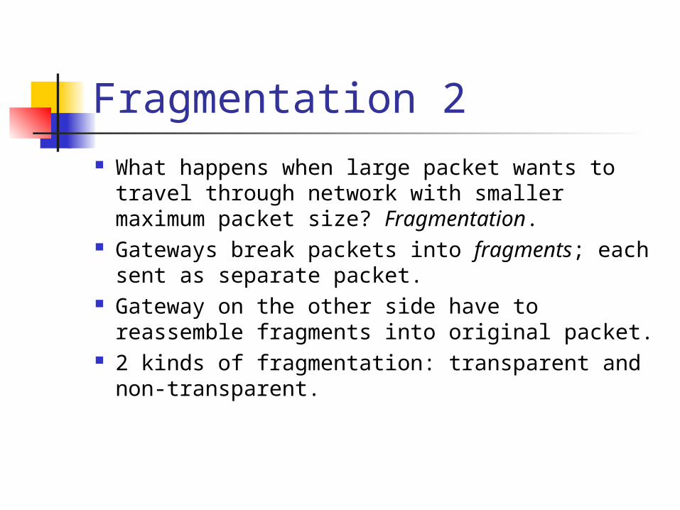
Fragmentation 2 What happens when large packet wants to

travel through network with smaller maximum packet size? Fragmentation.

Gateways break packets into fragments; each sent as separate packet.

Gateway on the other side have to reassemble fragments into original packet.

2 kinds of fragmentation: transparent and non-transparent.

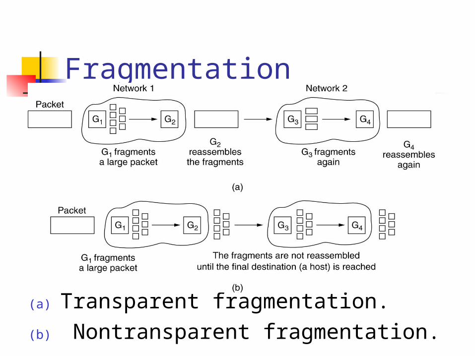
Fragmentation

(a) Transparent fragmentation. (b) Nontransparent fragmentation.

Fragmentation (2)

• Fragmentation when the elementary data size is 1 byte.• (a) Original packet, containing 10 data bytes.• (b) Fragments after passing through a network with

maximum packet size of 8 payload bytes plus header.• (c) Fragments after passing through a size 5 gateway.

Transparent Fragmentation

Small-packet network transparent to other subsequent networks.

Fragments of a packet addressed to the same exit gateway, where packet is reassembled. OK for concatenated VC internetworking.

Subsequent networks are not aware fragmentation occurred.

ATM networks (through special hardware) provide transparent fragmentation: segmentation.

Problems with Transparent Fragmentation

Exit gateway must know when it received all the pieces. - Fragment counter or “end of packet” bit.

Some performance penalty but requiring all fragments to go through same gateway.

May have to repeatedly fragment and reassemble through series of small-packet networks.

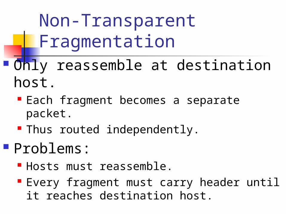
Non-Transparent Fragmentation

Only reassemble at destination host. Each fragment becomes a separate packet. Thus routed independently.

Problems: Hosts must reassemble. Every fragment must carry header until it

reaches destination host.

Keeping Track of Fragments 1 Fragments must be numbered so that

original data stream can be reconstructed.

Tree-structured numbering scheme: Packet 0 generates fragments 0.0, 0.1, 0.2, … If these fragments need to be fragmented later

on, then 0.0.0, 0.0.1, …, 0.1.0, 0.1.1, … But, too much overhead in terms of number of

fields needed. Also, if fragments are lost, retransmissions can

take alternate routes and get fragmented differently.

Keeping Track of Fragments 2

Another way is to define elementary fragment size that can pass through every network.

When packet fragmented, all pieces equal to elementary fragment size, except last one (may be smaller).

Packet may contain several fragments.

Keeping Track of Fragments 3 Header contains packet number, number of first

fragment in the packet, and last-fragment bit.

27 0 1 A B C D E F G H I J

27 0 0 A B C D E F G H 27 8 1 I J

Packet numberNumber offirst fragment

Last-fragment bit

(a) Original packetwith 10 data bytes.

(b) Fragments after passing through network with maximum packet size = 8 bytes.

1 byte