CM20145 Indexing and Hashing Dr Alwyn Barry Dr Joanna Bryson

CM20145CM20145Indexing and HashingIndexing and Hashing

Dr Alwyn BarryDr Joanna Bryson

Coursework Is Due on the Coursework Is Due on the 1616thth (Thursday)!! (Thursday)!!

Big Important Notice

Possible CW Plan (Lecture 10)Possible CW Plan (Lecture 10) This week:

G: write ER diagram, divy tables (~ 3hrs), I: write tables & populate a few rows.

`Reading’ week G: normalize/validate DB, divy reports (~ 3hrs), I: write reports / web pages.

Week of 22nd I: finish reports, link to others’, G: refactor DB, reports if necessary (~ 2hrs).

Week of 29th G: plan & divy hand-in report (~ 1hr), I: write hand-in.

Week of Dec. 6th G: Assemble hand-in, write communal credit page,

hand in (~0.5-4hr). Week of Dec. 13th

Laugh at unfinished groups.

More on the CourseworkMore on the Coursework Getting the group all together is the

hard part; my plan kept this down to 10 hours.

Individuals expected to spend at least as much time individually.

Point is for everyone to have built tables & reports in a large system.

Point is not shrinkwrapping. If an individual hasn’t turned up / done

their part, don’t feel obligated to cover the hole well, just document it.

Everyone has to sign final report!!

Last TimeLast Time Storage Access & Buffers File Organization

Fixed Length Records Variable Length

Organization of Records in Files Sequential & Clustering

Data-Dictionary Storage Intro to Indexing

Basic Concepts Ordered Indices

Dense & Sparse Multilevel Primary & Secondary

Now: Indexing & Hashing

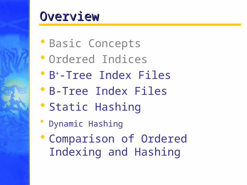
OverviewOverview

Basic Concepts Ordered Indices B+-Tree Index Files B-Tree Index Files Static Hashing Dynamic Hashing Comparison of Ordered Indexing

and Hashing

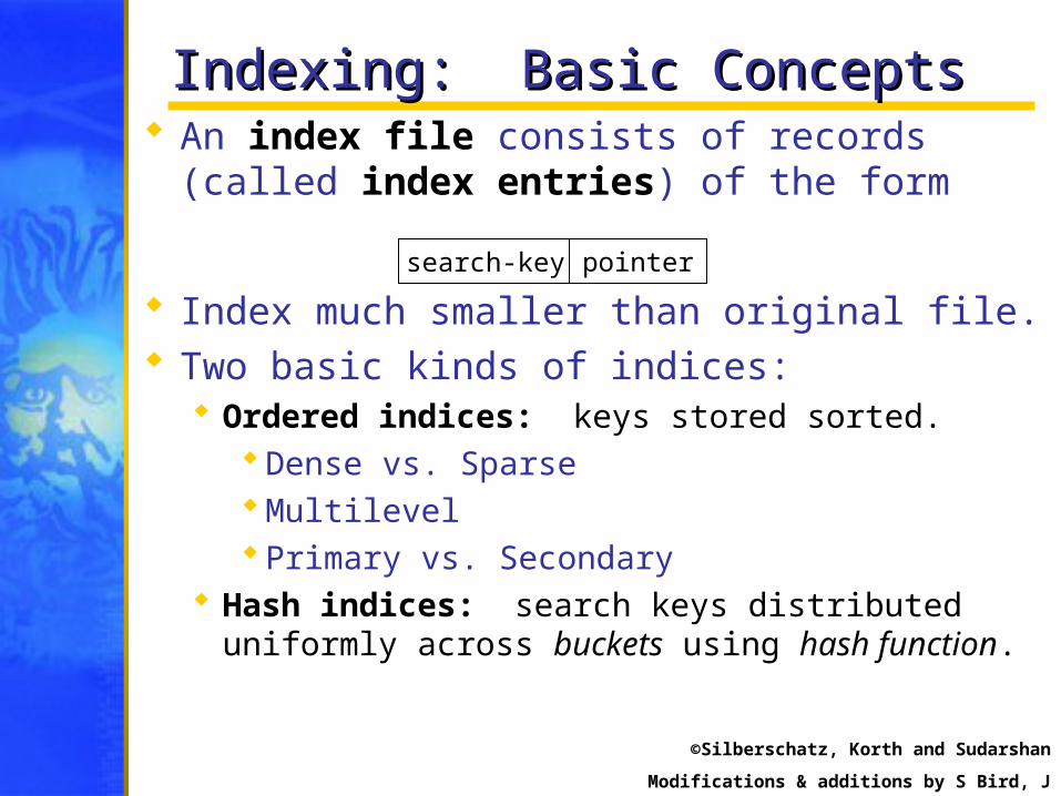
Indexing: Basic ConceptsIndexing: Basic Concepts An index file consists of records

(called index entries) of the form

Index much smaller than original file. Two basic kinds of indices:

Ordered indices: keys stored sorted.Dense vs. SparseMultilevelPrimary vs. Secondary

Hash indices: search keys distributed uniformly across buckets using hash function.

search-key pointer

©Silberschatz, Korth and Sudarshan

Modifications & additions by S Bird, J Bryson

Index Evaluation MetricsIndex Evaluation Metrics Types:

Access types supported efficiently. E.g., Records with a specified value in the

attribute.Records with an attribute value falling in

a specified range.

Time: Access time Insertion time Deletion time

Space: Space overhead

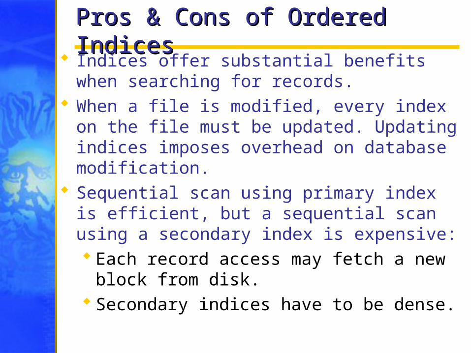
Pros & Cons of Ordered IndicesPros & Cons of Ordered Indices Indices offer substantial benefits when

searching for records. When a file is modified, every index on

the file must be updated. Updating indices imposes overhead on database modification.

Sequential scan using primary index is efficient, but a sequential scan using a secondary index is expensive: Each record access may fetch a new

block from disk. Secondary indices have to be dense.

OverviewOverview


and Hashing

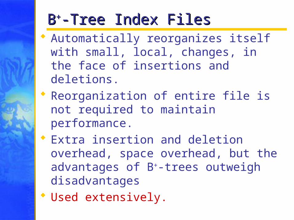
BB++-Tree Index Files-Tree Index Files Automatically reorganizes itself with

small, local, changes, in the face of insertions and deletions.

Reorganization of entire file is not required to maintain performance.

Extra insertion and deletion overhead, space overhead, but the advantages of B+-trees outweigh disadvantages

Used extensively.

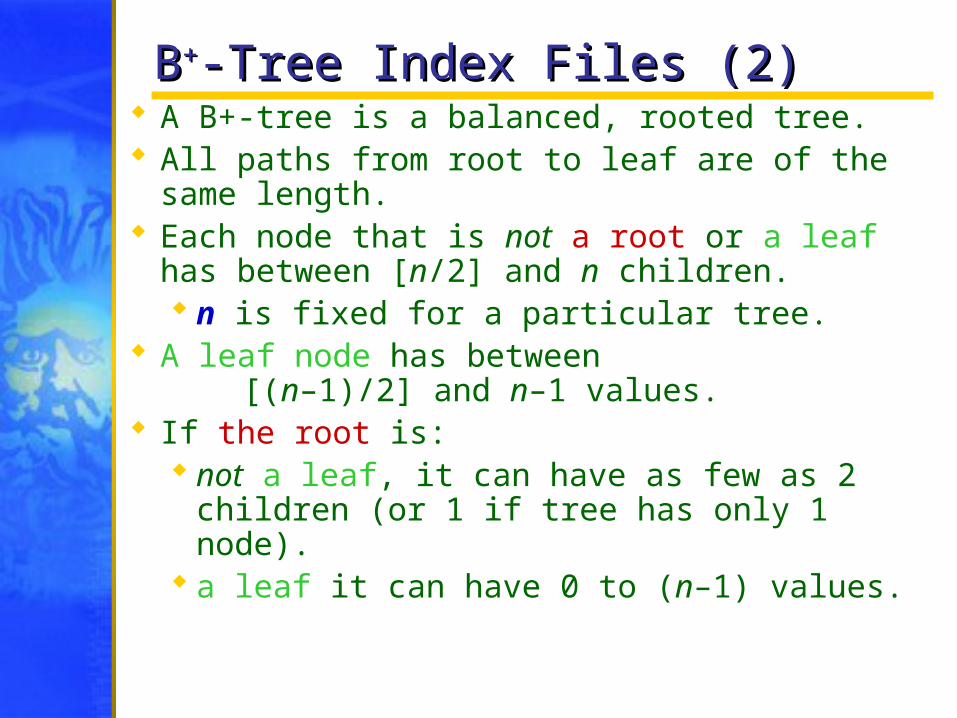
BB++-Tree Index Files (2)-Tree Index Files (2) A B+-tree is a balanced, rooted tree. All paths from root to leaf are of the

same length. Each node that is not a root or a leaf

has between [n/2] and n children.n is fixed for a particular tree.

A leaf node has between [(n–1)/2] and n–1 values.

If the root is: not a leaf, it can have as few as 2

children (or 1 if tree has only 1 node).

a leaf it can have 0 to (n–1) values.

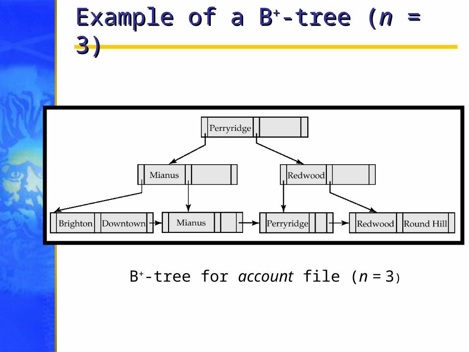
Example of a BExample of a B++-tree (-tree (nn = 3) = 3)

B+-tree for account file (n = 3)

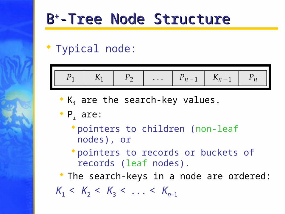
BB++-Tree Node Structure-Tree Node Structure

Typical node:

Ki are the search-key values.

Pi are:pointers to children (non-leaf nodes), orpointers to records or buckets of records

(leaf nodes). The search-keys in a node are ordered:

K1 < K2 < K3 < . . . < Kn–1

Example of a BExample of a B++-tree (-tree (nn = 3) = 3)


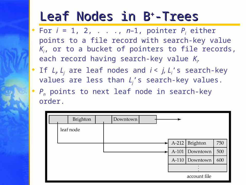
Leaf Nodes in BLeaf Nodes in B++-Trees-Trees For i = 1, 2, . . ., n–1, pointer Pi either points to

a file record with search-key value Ki, or to a bucket of pointers to file records, each record having search-key value Ki.

If Li, Lj are leaf nodes and i < j, Li’s search-key values are less than Lj’s search-key values.

Pn points to next leaf node in search-key order.

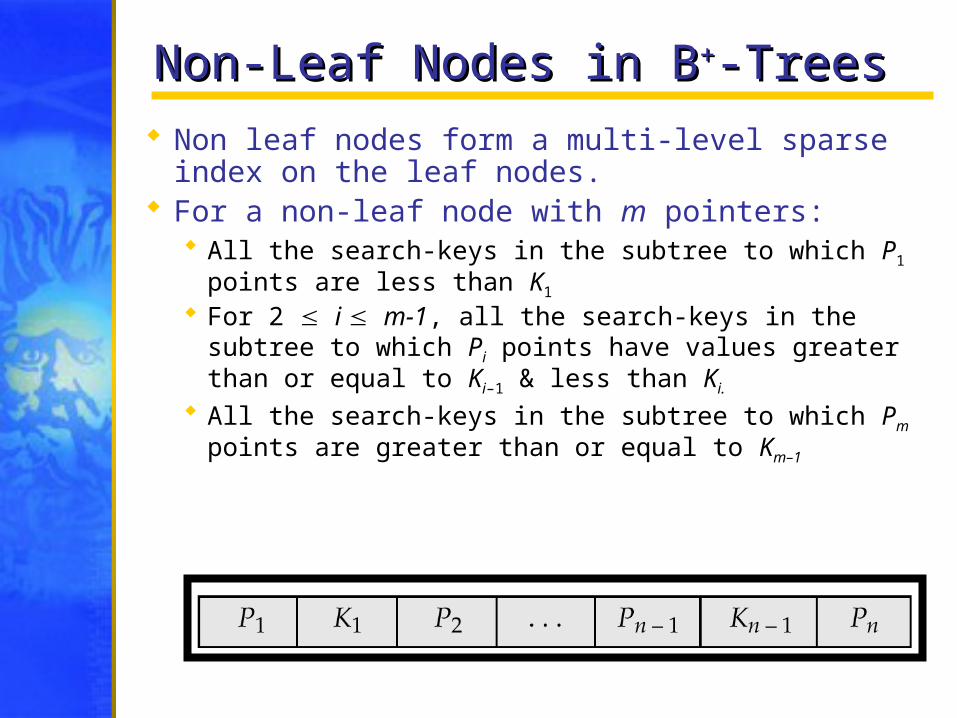
Non-Leaf Nodes in BNon-Leaf Nodes in B++-Trees-Trees Non leaf nodes form a multi-level sparse index

on the leaf nodes. For a non-leaf node with m pointers:

All the search-keys in the subtree to which P1 points are less than K1

For 2 i m-1, all the search-keys in the subtree to which Pi points have values greater than or equal to Ki–1 & less than Ki.

All the search-keys in the subtree to which Pm points are greater than or equal to Km–1

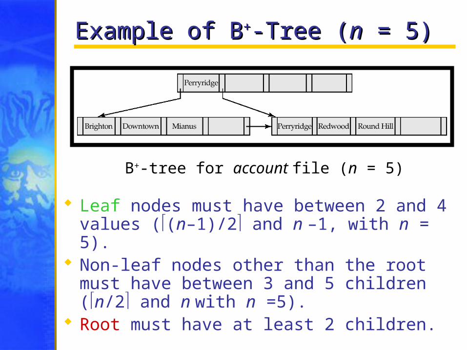
Example of BExample of B++-Tree (-Tree (nn = 5) = 5)

Leaf nodes must have between 2 and 4 values ((n–1)/2 and n –1, with n = 5).

Non-leaf nodes other than the root must have between 3 and 5 children (n/2 and n with n =5).

Root must have at least 2 children.


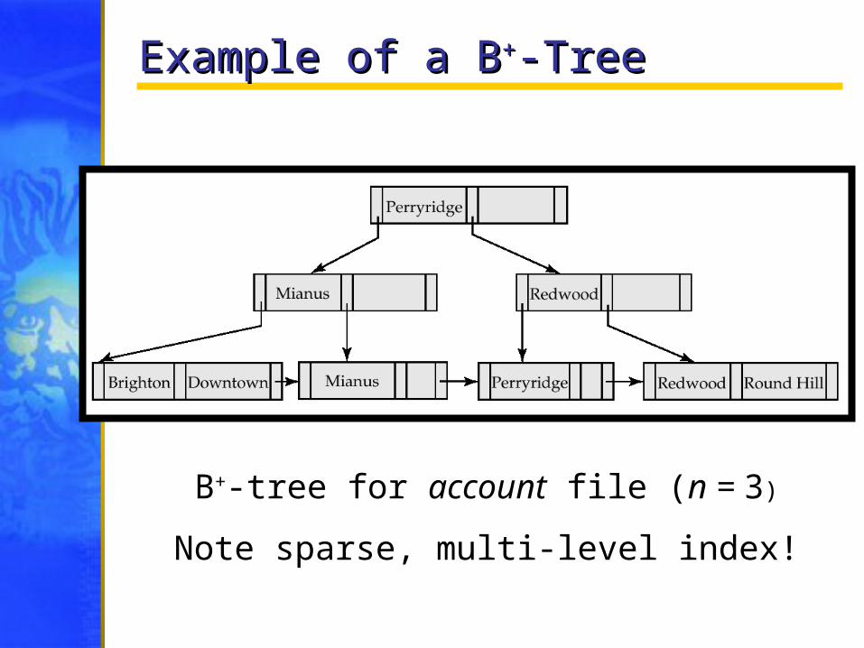
Example of a BExample of a B++-Tree-Tree


Note sparse, multi-level index!

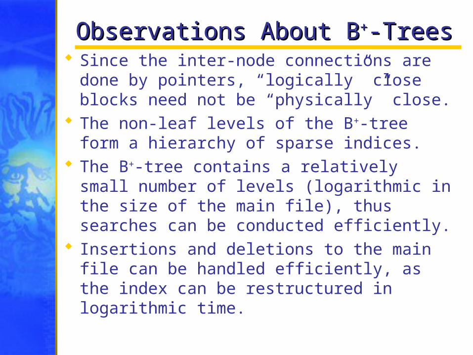
Observations About BObservations About B++-Trees-Trees Since the inter-node connections are

done by pointers, “logically” close blocks need not be “physically” close.

The non-leaf levels of the B+-tree form a hierarchy of sparse indices.

The B+-tree contains a relatively small number of levels (logarithmic in the size of the main file), thus searches can be conducted efficiently.

Insertions and deletions to the main file can be handled efficiently, as the index can be restructured in logarithmic time.

Queries on BQueries on B++-Trees-TreesFind all records with search-key value k.

1. Start with the root node:1. Examine the node for the smallest search-key value >

k.2. If such a value exists, assume it is Kj. Then follow Pi to

the child node3. Otherwise k Km–1, where there are m pointers in the

node. Then follow Pm to the child node.

2. If the node reached by following the pointer above is not a leaf node, repeat the above procedure on the node, and follow the corresponding pointer.

3. Eventually reach a leaf node. If for some i, key Ki = k follow pointer Pi to the desired record or bucket. Else no record with search-key value k exists.

Queries on BQueries on B++-Trees - Efficiency-Trees - Efficiency In processing a query, a path is traversed in the

tree from the root to some leaf node. If there are K search-key values in the file, the path

is no longer than logn/2(K). A node is generally the same size as a disk block,

typically 4 kilobytes, and n is typically around 100 (40 bytes per index entry).

With 1 million search key values and n = 100, at most log50(1,000,000) = 4 nodes are accessed in a lookup.

Contrast this with a balanced binary tree with 1 million search key values — around 20 nodes are accessed in a lookup — this difference is significant since every node

access may need a disk I/O, costing around 20 milliseconds!

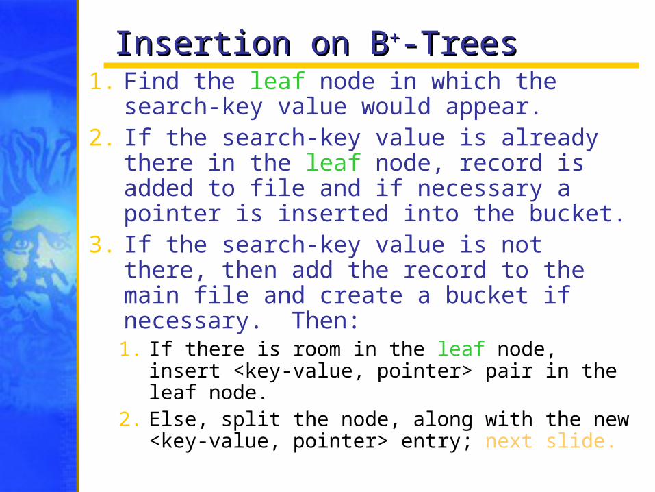
Insertion on BInsertion on B++-Trees-Trees1. Find the leaf node in which the search-

key value would appear.2. If the search-key value is already there

in the leaf node, record is added to file and if necessary a pointer is inserted into the bucket.

3. If the search-key value is not there, then add the record to the main file and create a bucket if necessary. Then:1. If there is room in the leaf node, insert

<key-value, pointer> pair in the leaf node.2. Else, split the node, along with the new

<key-value, pointer> entry; next slide.

Insertion on BInsertion on B++-Trees (2)-Trees (2) Splitting a node:

1. Take the n pairs (including the new one) <search-key value, pointer> in sorted order.

2. Leave the first n/2 in original node, place the rest in a new node.

3. Let the new node be p, and let k be the least key value in p. 1. Insert <k,p> in the parent of the node

being split. 2. If the parent is full, split it and propagate

the split further up. The splitting of nodes proceeds upwards until

a node that is not full is found. Worst case: the root node may be split,

increasing the height of the tree by 1.

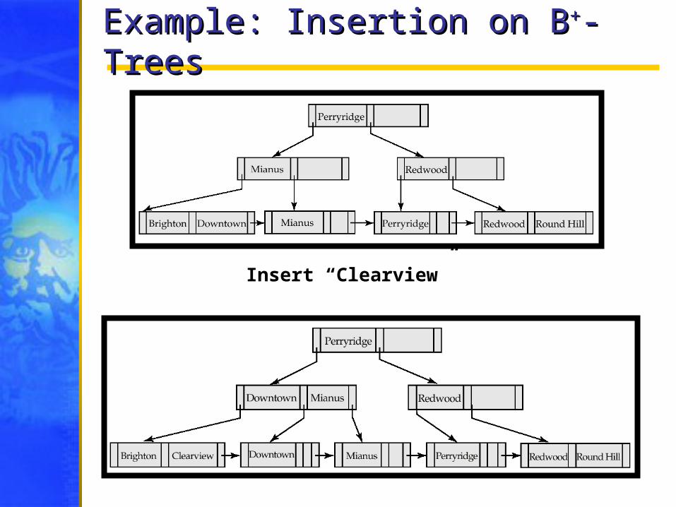
Example: Insertion on BExample: Insertion on B++-Trees-Trees

Insert “Clearview”

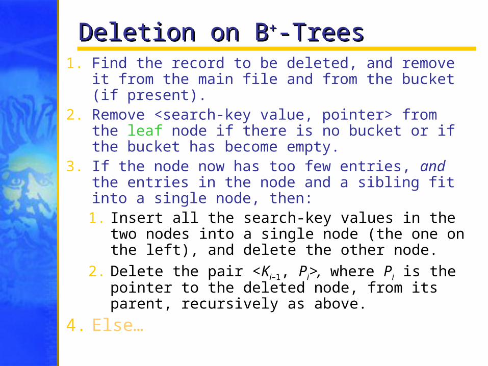
Deletion on BDeletion on B++-Trees-Trees1. Find the record to be deleted, and remove it

from the main file and from the bucket (if present).

2. Remove <search-key value, pointer> from the leaf node if there is no bucket or if the bucket has become empty.

3. If the node now has too few entries, and the entries in the node and a sibling fit into a single node, then: 1. Insert all the search-key values in the two

nodes into a single node (the one on the left), and delete the other node.

2. Delete the pair <Ki–1, Pi>, where Pi is the pointer to the deleted node, from its parent, recursively as above.

4. Else…

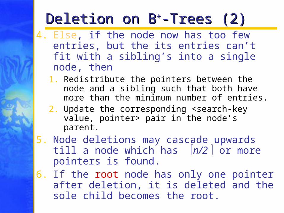
Deletion on BDeletion on B++-Trees (2)-Trees (2)4. Else, if the node now has too few

entries, but the its entries can’t fit with a sibling’s into a single node, then

1. Redistribute the pointers between the node and a sibling such that both have more than the minimum number of entries.

2. Update the corresponding <search-key value, pointer> pair in the node’s parent.

5. Node deletions may cascade upwards till a node which has n/2 or more pointers is found.

6. If the root node has only one pointer after deletion, it is deleted and the sole child becomes the root.

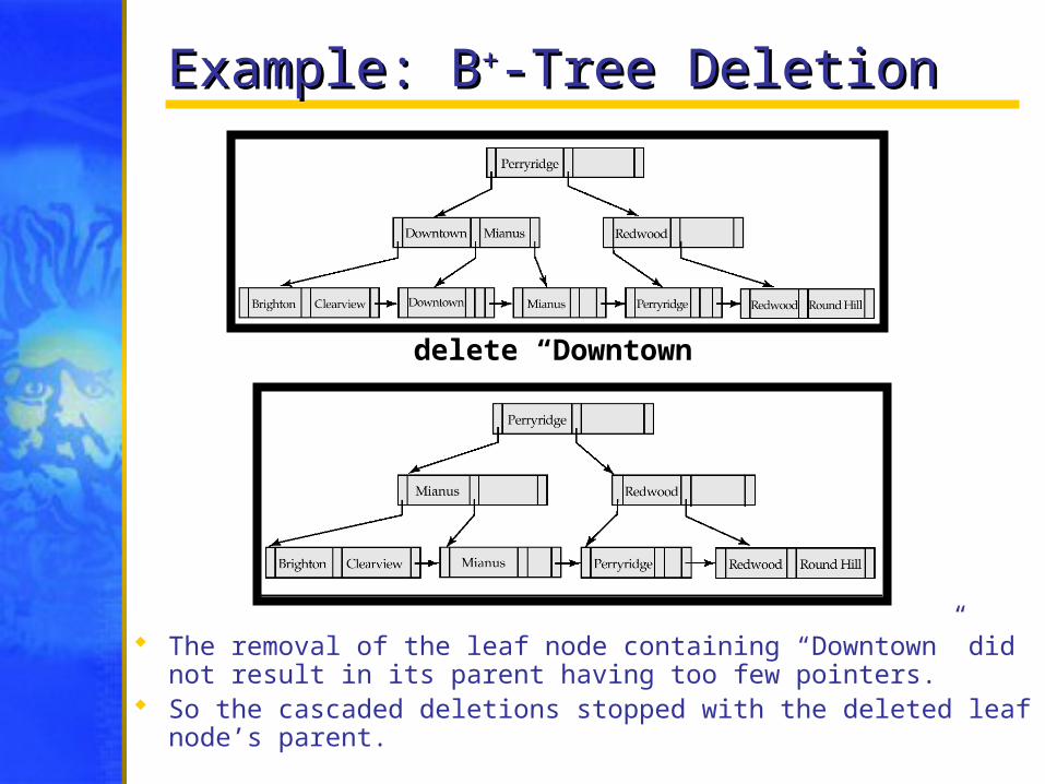
Example: BExample: B++-Tree Deletion-Tree Deletion

The removal of the leaf node containing “Downtown” did not result in its parent having too few pointers.

So the cascaded deletions stopped with the deleted leaf node’s parent.

delete “Downtown”

Example 2: BExample 2: B++-Tree Deletion-Tree Deletion

I. Node with “Perryridge” becomes underfull (empty in this case) and merged with its sibling.

II. As a result “Perryridge” node’s parent became underfull, and was merged with its sibling (and an entry was deleted from their parent).

III. Root node then had only one child, and was deleted and its child became the new root node.

Delete “Perryridge”

Example 3: BExample 3: B++-tree Deletion-tree Deletion

Parent of leaf containing Perryridge became underfull, and borrowed a pointer from its left sibling.

Search-key value in the parent’s parent changes as a result.

Delete “Perryridge”

OverviewOverview


and Hashing

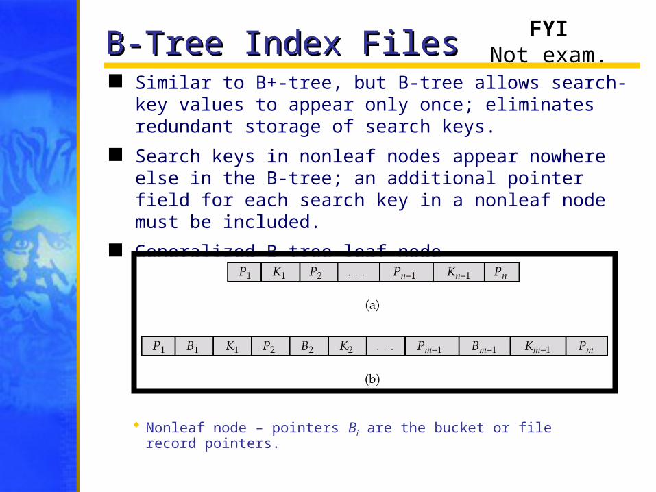
B-Tree Index FilesB-Tree Index Files Similar to B+-tree, but B-tree allows search-key values to

appear only once; eliminates redundant storage of search keys.

Search keys in nonleaf nodes appear nowhere else in the B-tree; an additional pointer field for each search key in a nonleaf node must be included.

Generalized B-tree leaf node

Nonleaf node – pointers Bi are the bucket or file record pointers.

FYINot exam.

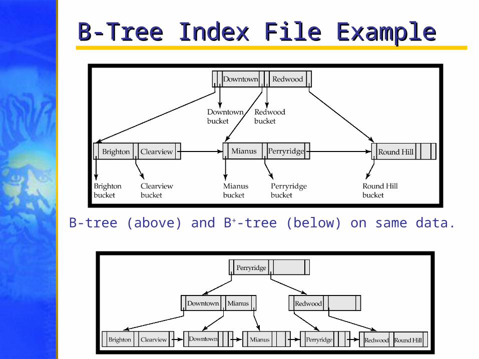
B-Tree Index File ExampleB-Tree Index File Example

B-tree (above) and B+-tree (below) on same data.

B-Tree B-Tree vs.vs. B B++-Tree Indices-Tree Indices Advantages of B-Tree indices:

May use less tree nodes than a corresponding B+-Tree. Sometimes possible to find search-key value before

reaching leaf node.

Disadvantages of B-Tree indices: Only small fraction of all search-key values are found

early. Non-leaf nodes are larger, so fan-out is reduced:

Thus B-Trees typically have greater depth than corresponding B+-Tree.

Insertion, deletion more complicated than in B+-Trees. Implementation is harder than B+-Trees.

Typically, advantages of B-Trees do not outweigh disadvantages.

OverviewOverview


and Hashing

Static HashingStatic Hashing A bucket is a unit of storage containing one or

more records (typically a disk block). Hash file organization: obtain the record’s

bucket directly from its search-key value using a hash function.

Hash function h is a function from the set of all search-key values K to the set of all bucket addresses B.

Hash function is used to locate records for access, insertion as well as deletion.

Records with different search-key values may be mapped to the same bucket;

so entire bucket has to be searched sequentially to locate a record.

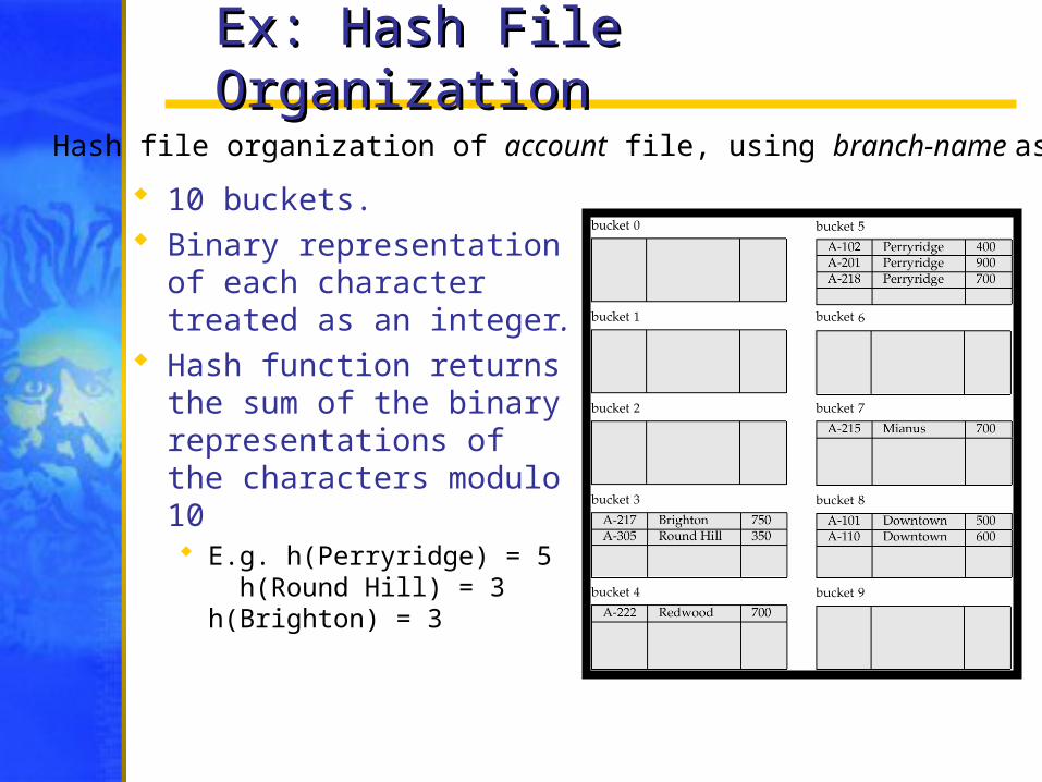
Ex: Hash File OrganizationEx: Hash File Organization

10 buckets. Binary representation

of each character treated as an integer.

Hash function returns the sum of the binary representations of the characters modulo 10 E.g. h(Perryridge) = 5

h(Round Hill) = 3 h(Brighton) = 3

Hash file organization of account file, using branch-name as key

Hash FunctionsHash Functions Worst hash function maps all search-key values

to the same bucket; this makes access time proportional to the number of search-key values in the file.

Ideal hash function is uniform – each bucket is assigned the same number of search-key values from the set of all possible values.

Ideal hash function is random, so each bucket will have the same number of records assigned to it irrespective of the actual distribution of search-key values in the file.

Typical hash functions perform computation on the internal binary representation of the search-key.

Bucket OverflowBucket Overflow

Bucket overflow can occur because of: Insufficient buckets Skewed distribution of records:

multiple records have same search-key value, or

chosen hash function produces non-uniform distribution of key values.

The probability of bucket overflow can be reduced, but not eliminated.

Handled by using overflow buckets.

FYINot exam.

Bucket OverflowBucket Overflow

Overflow chaining – the overflow buckets of a given bucket are chained together in a linked list.

FYINot exam.

Deficiencies of Static HashingDeficiencies of Static Hashing In static hashing, function h maps search-key

values to a fixed set of B of bucket addresses. Databases grow with time. If initial number of

buckets is too small, performance will degrade due to too many overflows.

If file size at some point in the future is anticipated and number of buckets allocated accordingly, significant amount of space will be wasted initially.

If database shrinks, again space will be wasted. One option is periodic re-organization of the file with

a new hash function, but it is very expensive. Run at night, holidays, on mirror…

These problems can be avoided by using techniques that allow the number of buckets to be modified dynamically.

Dynamic HashingDynamic Hashing Allows dynamic modification of hash function. Good for database that often changes size. Extendable hashing – one form of dynamic

hashing Hash function generates values over a large range —

typically b-bit integers, with b = 32. At any time use only a prefix of the hash function to index

into a table of bucket addresses. Let the length of the prefix be i bits, 0 i 32. Bucket address table size = 2i. Initially i = 0 Value of i grows and shrinks as the size of the database

grows and shrinks. Multiple entries in the bucket address table may point to a

bucket. Thus, actual number of buckets is < 2i

The number of buckets also changes dynamically due to coalescing and splitting of buckets.

See SKS 12.6 for full details about queries and updates.

FYINot exam.

Extendable Hashing: Pro and ConExtendable Hashing: Pro and Con Benefits of extendable hashing:

Hash performance does not degrade with growth of file.

Minimal space overhead. Disadvantages of extendable hashing

Extra level of indirection to find desired record.

Bucket address table may itself become very big (larger than memory)Need a tree structure to locate desired

record in the structure! Changing size of bucket address table is

an expensive operation.

SummarySummary


and Hashing

Next: Queries & Optimization

Ordered Indexing Ordered Indexing vs.vs. Hashing Hashing Cost of periodic re-organization. Relative frequency of insertions and

deletions vs. simple queries. Is it desirable to optimize average

access time at the expense of worst-case access time?

Expected type of queries: Hashing is generally better at retrieving

records having a specified value of the key. If range queries are common, ordered

indices are to be preferred.

SummarySummary


and Hashing

Next: Queries & Optimization

Reading & ExercisesReading & Exercises

Reading Silberschatz Chapters 12 Connolly & Begg C.4, C.5.5, C.7

Exercises: Silberschatz 12.1-8, 16 Think about the algorithms behind

building & maintaining B+ trees, hashes.

End of TalkEnd of Talk

The following slides are ones I might use next year. They were not presented in class

and you are not responsible for them.

JJB Dec 2003

BB++-Tree File Organization-Tree File Organization Index file degradation problem is solved by

using B+-Tree indices. Data file degradation problem is solved by

using B+-Tree File Organization. The leaf nodes in a B+-tree file organization

store records, instead of pointers. Since records are larger than pointers, the

maximum number of records that can be stored in a leaf node is less than the number of pointers in a nonleaf node.

Leaf nodes are still required to be at least half full.

Insertion and deletion are handled in the same way as insertion and deletion of entries in a B+-tree index.

Hash IndicesHash Indices Hashing can be used for

both file organization and index-structure creation.

A hash index organizes the search keys, with their associated record pointers, into a hash file structure.

If the file itself is organized using hashing, a separate primary hash index on it using the same search-key is unnecessary. We use the term hash index

to refer to both secondary index structures and hash organized files.

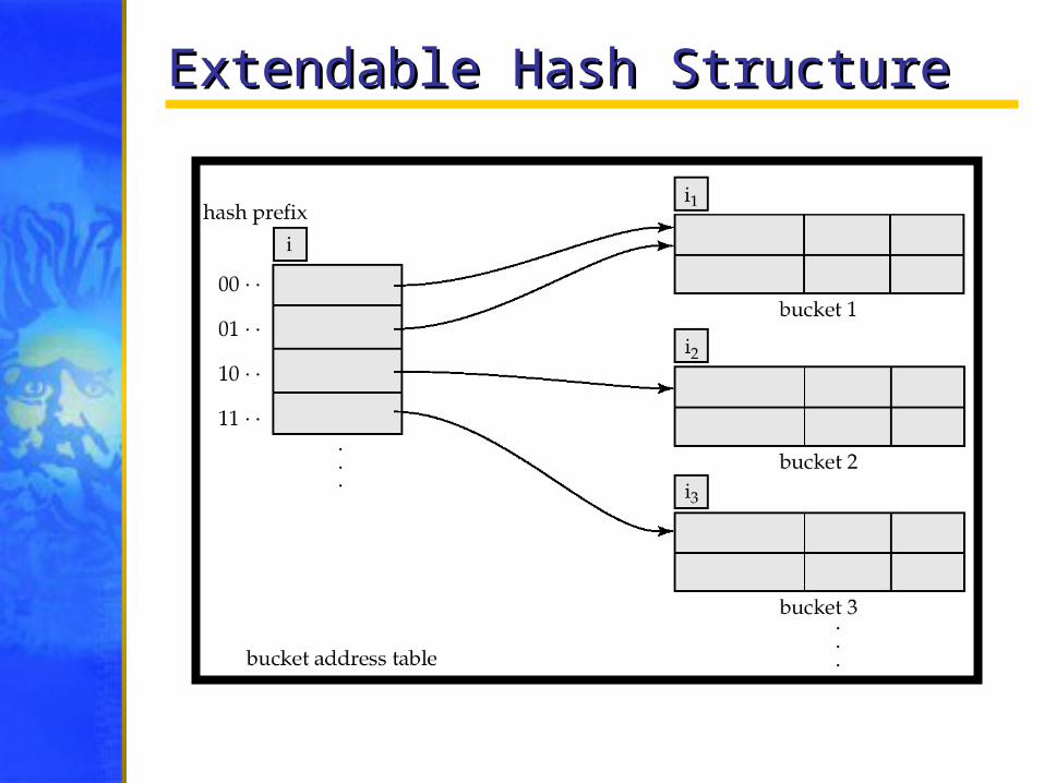
Extendable Hash Structure Extendable Hash Structure

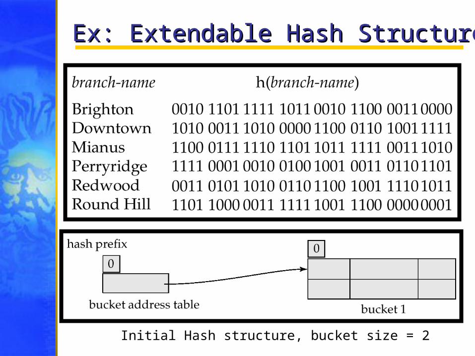
Ex: Extendable Hash StructureEx: Extendable Hash Structure

Initial Hash structure, bucket size = 2

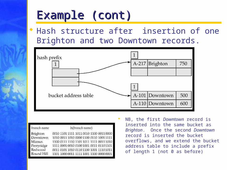
Example (cont)Example (cont) Hash structure after insertion of one

Brighton and two Downtown records.

NB, the first Downtown record is inserted into the same bucket as Brighton. Once the second Downtown record is inserted the bucket overflows, and we extend the bucket address table to include a prefix of length 1 (not 0 as before)

Example (cont)Example (cont)Hash structure after insertion of Mianus record

Example (cont)Example (cont)

Hash structure after insertion of three Perryridge records

NB, the bucket overflow with Perryridge cannot be solved by enlarging the hash prefix used in the bucket address table, so instead we are forced to use an overflow bucket

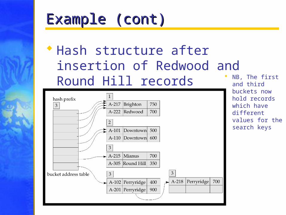
Example (cont)Example (cont)

Hash structure after insertion of Redwood and Round Hill records

NB, The first and third buckets now hold records which have different values for the search keys

Documents

CM20145 Indexing and Hashing Dr Alwyn Barry Dr Joanna Bryson