1

3

2

Clustering Time Series using Unsupervised-Shapelets

Jesin Zakaria Abdullah Mueen Eamonn Keogh

Department of Computer Science and Engineering

University of California, Riverside

{jzaka001, mueen, eamonn}@cs.ucr.edu

Abstract— Time series clustering has become an increasingly

important research topic over the past decade. Most existing

methods for time series clustering rely on distances calculated

from the entire raw data using the Euclidean distance or

Dynamic Time Warping distance as the distance measure.

However, the presence of significant noise, dropouts, or

extraneous data can greatly limit the accuracy of clustering in

this domain. Moreover, for most real world problems, we

cannot expect objects from the same class to be equal in length.

As a consequence, most work on time series clustering only

considers the clustering of individual time series “behaviors,”

e.g., individual heart beats or individual gait cycles, and

contrives the time series in some way to make them all equal in

length. However, contriving the data in such a way is often a

harder problem than the clustering itself.

In this work, we show that by using only some local

patterns and deliberately ignoring the rest of the data, we can

mitigate the above problems and cluster time series of different

lengths, i.e., cluster one heartbeat with multiple heartbeats. To

achieve this we exploit and extend a recently introduced

concept in time series data mining called shapelets. Unlike

existing work, our work demonstrates for the first time the

unintuitive fact that shapelets can be learned from unlabeled

time series. We show, with extensive empirical evaluation in

diverse domains, that our method is more accurate than

existing methods. Moreover, in addition to accurate clustering

results, we show that our work also has the potential to give

insights into the domains to which it is applied.

Keywords-time series; clustering; shapelets; unsupervised

I. INTRODUCTION

Time series analysis is an important topic within many fields of research including, aerospace, finance, business, meteorology, medical science, motion capture, etc. [8][26][34]. However, most research on time series analysis is limited by the need for costly labeled data. This has led to an increase of interest in clustering time series data, which, by definition, does not require access to labeled data [33][8][4][9].

A decade old empirical comparison by Keogh and Kasetty in [11] reveals the somewhat surprising fact that the simple Euclidean distance metric is highly competitive with other more sophisticated distance measures, and more recent work confirms this [3]. However, the time series must be of equal length for the Euclidean distance to be defined. Dynamic Time Warping (DTW) can both solve this problem and handle the difficulty of clustering time series containing out-of-phase similarities as shown in [12][1][25][3].

In this work, however, we argue that the apparent utility of Euclidean distance or DTW for clustering may come from an over dependence on the UCR time series archive [13], for

testing clustering algorithms [33][12][19]. The problem is that the data in this archive has already been hand-edited to have equal length and (approximate) alignment. However, the task of contriving the data in this format is almost certainly harder than the task of giving labels to the data, i.e., the clustering itself.

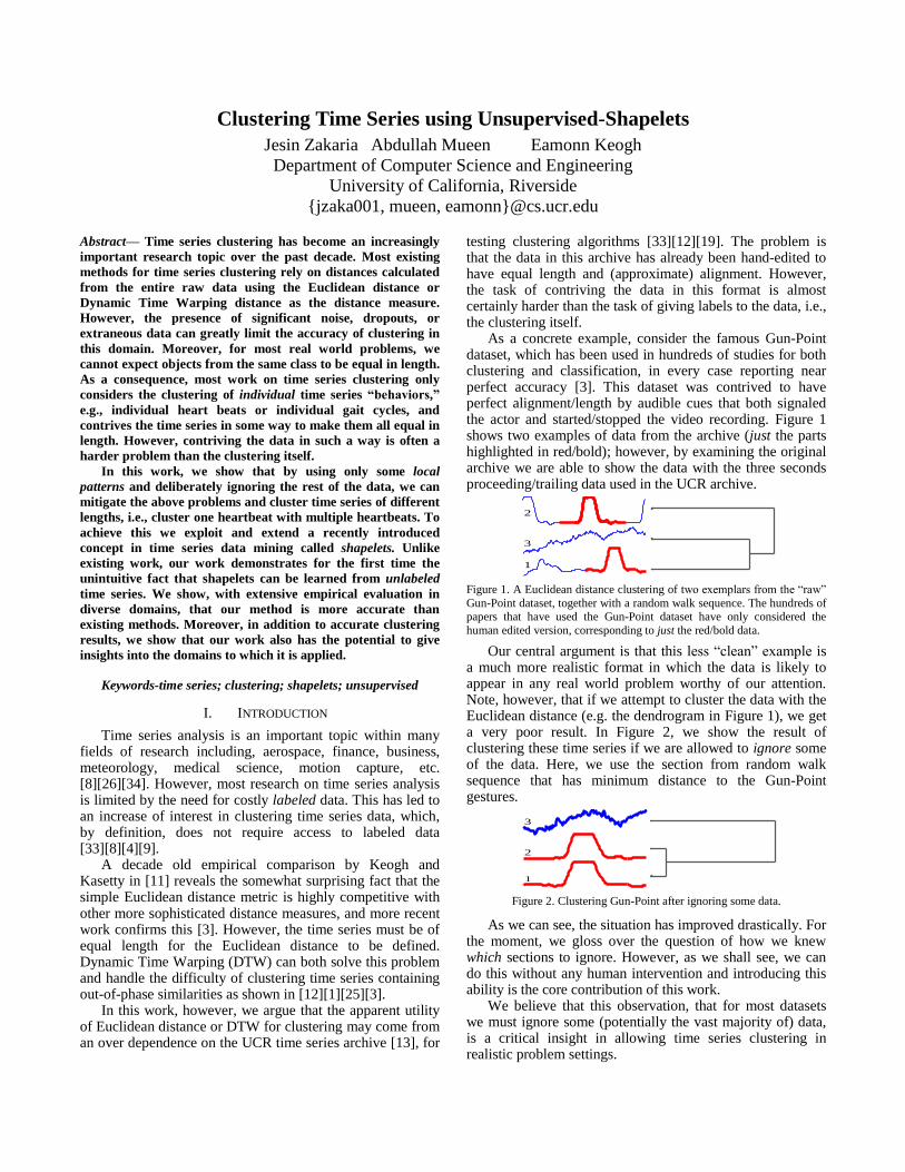
As a concrete example, consider the famous Gun-Point dataset, which has been used in hundreds of studies for both clustering and classification, in every case reporting near perfect accuracy [3]. This dataset was contrived to have perfect alignment/length by audible cues that both signaled the actor and started/stopped the video recording. Figure 1 shows two examples of data from the archive (just the parts highlighted in red/bold); however, by examining the original archive we are able to show the data with the three seconds proceeding/trailing data used in the UCR archive.

Figure 1. A Euclidean distance clustering of two exemplars from the “raw”

Gun-Point dataset, together with a random walk sequence. The hundreds of papers that have used the Gun-Point dataset have only considered the

human edited version, corresponding to just the red/bold data.

Our central argument is that this less “clean” example is a much more realistic format in which the data is likely to appear in any real world problem worthy of our attention. Note, however, that if we attempt to cluster the data with the Euclidean distance (e.g. the dendrogram in Figure 1), we get a very poor result. In Figure 2, we show the result of clustering these time series if we are allowed to ignore some of the data. Here, we use the section from random walk sequence that has minimum distance to the Gun-Point gestures.

Figure 2. Clustering Gun-Point after ignoring some data.

As we can see, the situation has improved drastically. For the moment, we gloss over the question of how we knew which sections to ignore. However, as we shall see, we can do this without any human intervention and introducing this ability is the core contribution of this work.

We believe that this observation, that for most datasets we must ignore some (potentially the vast majority of) data, is a critical insight in allowing time series clustering in realistic problem settings.

1

2

3

We are aware of the “chicken-and-egg” nature of our claim. We must ignore some data to allow a good clustering, and a good clustering is the obvious way to reveal the best data to keep (and ignore). However, we will show that time series shapelets [32] can be adapted to resolve this paradox.

Time series shapelets are small, local patterns in a time series that are highly predictive of a class. The idea of shapelets was introduced by Ye [32] as a primitive for time series data mining. Since then, numerous other researchers have shown the utility of shapelets for classifying time series data [21][16][7][30].

In this work, we show for the first time that shapelets can also be highly competitive in clustering time series data. Since we do not know the labels of the time series in the dataset, this begs the question, “How can we discover shapelets from a dataset without having any knowledge of the class labels?” We propose a new form of shapelet that we call unsupervised-shapelet (or u-shapelet) and demonstrate its utility for clustering time series data.

The rest of the paper is organized as follows: In Section 2 we define the necessary notation; in Section 3, we discuss previous work on clustering time series; Section 4 explains our method for obtaining shapelets in the absence of class labels; Section 5 shows forceful empirical evidence of our algorithm working on many datasets from diverse domains; lastly, Section 6 concludes and gives direction of future research.

II. DEFINITIONS AND BACKGROUND

We present the definitions of key terms that we use in this work. For our problem, each object in the dataset is a time series, which may be of different lengths.

Definition 1: Time Series, a time series T = T1, T2, …, Tn is an ordered set of real values. The total number of real values is equal to the length of the time series. A dataset D = {T1, T2, … TN} is a collection of N such time series.

In this work, we demonstrate that if we can find small subsequences of few time series that best represent their clusters (e.g. red/bold subsequences of Figure 1), then those subsequences may give us a better clustering result than using the entire time series.

Definition 2: Subsequence, a subsequence Si,l, where 1≤l≤n and 1≤i≤n, is a set of l continuous real values from a time series, T, that starts at position i.

For a time series of length n, there can be in total,

subsequences of all possible lengths. If there are N time series in the dataset with length n, then there will be in total,

subsequences.

Previous research efforts on shapelet discovery [32][21],

had to consider all the

subsequences to find

optimal shapelets for building the classifier. However, as we shall see, we need to explore only a tiny subset of these subsequences to find the optimal u-shapelets.

Our clustering algorithm thus inherits much of the discriminating power of shapelets, but little of their well-documented lethargy. We will formalize the definition of u-shapelets shortly.

We can compute the distance between two time series of equal length, by simply calculating the Euclidean distance between them. To make our distance measure invariant to scale and offset, we need to z-normalize the time series before computing their Euclidean distance. As demonstrated in [11], even tiny differences in scale and offset rapidly swamp any similarity in shape.

In order to compare or rank candidate u-shapelets we need to consider the utility (i.e. discriminating power) of subsequences of different lengths, as in most cases we expect the distance between shorter subsequences will be less than the distance between longer subsequences. Thus we normalize the distance by the length of the subsequence. We call this the length-normalized Euclidean distance. The length-normalized Euclidean distance between two time series and can be computed using,

√

∑

which takes time linear on the length

of the time series. We can reduce the amortized time complexity of this

calculation from linear to constant by caching the results of some calculations. The five results to cache

are∑ ,∑

,∑

, ∑

, and ∑

. This method has been adopted and described in [21]. For brevity, we refer the interested reader to that work [21]. Using these numbers we can compute the mean µ (1) and standard deviation (std) σ (2).

∑

∑

The positive correlation (3) and the length-normalized Euclidean distance (4) can be computed as follows [22].

∑

√ ( )

We are now in a position to explain how we calculate the distance between a (typically short) subsequence S and a (typically much longer) time series T. We need to “slide” S against T to find the alignment that minimizes the distance.

Definition 3: The Subsequence distance between a subsequence S of length m and a time series T of length n is the distance between S and the subsequence of T that has minimum distance. We denote it as sdist(S, T).

Note that we generally expect m << n, and that both sdist(S, T) and sdist(T, S) are only defined if n = m.

In previous works, a definition similar to sdist was used to support a definition of shapelets; small subsequences that separate time series into two or more distinct groups by their “nearness” or “distance” to that subsequence [32][21]. Since we cannot use the class labels of the time series to discover the shapelets, we call our definition of informative subsequences unsupervised-shapelets or u-shapelets to

differentiate them from the classic shapelets which assume access to class labels [32][21].

Definition 4: An unsupervised-shapelet is a subsequence of a time series T for which the sdists

between and the time series from a group DA are much

smaller than the sdists between and rest of the time series DB in the dataset D (6).

We will expound on how we formalize “much smaller” below. The reader may wonder how we identify DA and DB without class labels. In Section IV.B we have formalized an algorithm to discover u-shapelets from a dataset. The algorithm will rigorously clarify the concept of DA and DB, so we defer a detailed discussion about it until then.

Note that, unlike the trivial example shown in Figure 2, many problems may require more than one u-shapelet. Thus we need to generalize our representation to allow for multiple u-shapelets. We call the matrix that contains the sdists vectors between u-shapelets and each time series in the dataset a Distance map.

Definition 5: A Distance map contains the sdists between each of the u-shapelets and all the time series in the dataset. If we have m u-shapelets for a dataset of N time series, the size of the distance map is [N × m] where each column is a distance vector of a u-shapelet.

For any dataset, once we have this distance map of the u-shapelets’ distances, we can simply pass it into an off-the-shelf clustering algorithm such as k-means. Thus the focus of our work is in algorithms for obtaining high quality distance maps. Note that the distance map representation is somewhat similar to the vector space model, which is a cornerstone of most text mining algorithms [27].

A. A Discrete Analogue of U-Shapelet

In order to enhance the reader’s understanding of u-shapelets and to lay the groundwork for the intuition about our proposed distance map building method, we present a very simple example from a discrete (rather than real-valued) sequence domain. This example is a close analogue of the task at hand. The use of the discrete data simply allows us to explain our ideas in a domain where the reader’s intuitions are highly developed and without the need of resorting to figures.

Consider the following collection of phrases, which is an analogue of a dataset of time series:

San Jose; Earth Day; San Francisco; Memorial Day; Fink Nottle; Labor Day; Bingo Little.

If we are asked to cluster this set of phrases into three groups, then as intuitive humans we would almost certainly split the data based on the presence/absence of the two substrings “San” and “Day”.

However, doing this algorithmically is a little more challenging. Since the phrases differ in length, we cannot apply Hamming distance, which is analogous to Euclidean distance, to compute the distance vector of the full phrases. The problem of length difference is solved by using Edit distance, which is the discrete version of DTW, but the Edit

distance produces a clustering that looks essentially random, as it needs to “explain” the irreverent sections e.g., Earth, Francisco, Memorial etc.

Instead, we can try to find representative substrings of the above phrases. By visual inspection the obvious candidates are “San” and “Day”. We compute the Hamming distances of these words to their nearest substrings in all phrases, and produce the distance map shown in Table I.

TABLE I. DISTANCE MAP OF “DAY” AND “SAN”

San Jose Earth Day San Fran.. Mem.. Day Fink Nottle Labor Day Bingo Little

San 0 2 0 2 2 2 2

Day 2 0 2 0 3 0 3

Using this distance map, we can cluster the phrases perfectly by using k-means on the columns. Moreover, examining the key-phrases (u-shapelet analogues) chosen for clustering gives us some intuition about the domain. For example, we may notice that the second, fourth, and sixth phrases are some kinds of “day”.

The above example is rather simple and the reader may wonder if this method works only if some u-shapelets have zero distance to the nearest neighbors of their own group. The answer is no, this method can handle more complex datasets. Consider the following set of sentences,

Abraham Lincoln lived here for many years. (English) She is looking for Ibrahim. (Arabic) You can find Abrahan in that house. (Portuguese) Michael is singing a song for her. (English) She bought a gift for Michaël. (Dutch) She can teach Michales chess (Hebrew)

The Hamming distances from the key-phrase Abraham to its nearest neighbors is [0, 2, 1, 7, 7, 7] respectively, and this distance vector is only entry necessary in a distance map that can cluster the sentences correctly into two groups. Note, however, that the choice of Abraham is somewhat arbitrary, as the data can also be correctly clustered by using either the similar key-phases Ibrahim/Abrahan or by any of the three variants of Michael.

We conclude this section by summarizing what we have learned from this analogy. First of all, to cluster data, we are

generallysomewhat paradoxicallybetter off ignoring large sections of the data. Secondly, while sometimes a single key element (i.e. Abraham) may be enough to separate the data into meaningful clusters, in some cases we may need two or more (i.e. Day and San) elements to separate the data.

III. RELATED WORK

The literature on clustering time series is vast; we refer the reader to [14] which offers a useful survey. Much of the work can be broadly classified into two categories:

Shape-based clustering, which attempts to cluster the data based on the shape of the entire time series [4], using Euclidean distance, DTW, or one of a host of other distance measures [3]. Note that our method contrasts with these ideas in that we explicitly allow our representation to ignore much of the data.

Statistical-based clustering, which attempts to cluster the data based on statistical features extracted from the time series. These features include common measures

such as mean, standard deviation, skewness, etc., in addition to more exotic features such as coefficients of ARIMA models [10], and fractal measures [29], etc.

One problem with the latter approaches is that they typically require a great many parameters and (at least apparently) ad-hoc choices. The problem with the former approaches is that the distance measures consider all data points, even though (as hinted in Figure 1 and Figure 2) we may be better off ignoring much of the data. Note that there are a handful of methods that combine both ideas by using statistics/features which are derived from time series shapes [8][34][3] .

The work closest to ours in spirit is that of Rakthanmanon et al., which shows the importance of ignoring some data for clustering within a single time series stream [23].

IV. OUR ALGORITHM

We are finally in a position to present a more direct insight and formal description of our algorithm.

A. An Intuition of our Clustering Algorithm

Consider the Trace dataset from the UCR archive [13]. It contains 50 instances from each of four classes, all with a length of 275. In Figure 3, we present ten random instances from each class. Note that while the global patterns within each class are the same, they are not aligned perfectly. As a result, if we use entire time series for k-means clustering with the Euclidean distance as distance measure, we will get poor results (we formally measure the quality of the results using the Rand index in the experimental section below, for the moment it is suffice to note the results are poor).

Figure 3. Sample time series from four classes of Trace dataset.

However, suppose that we use subsequences that are prominent in one class but not in other classes as u-shapelets (e.g. the red subsequences in Figure 4 (left). We can then use their distance map to separate all the time series. In Figure 4 (right), we plot the distance map of the two u-shapelets in two-dimensional space. In this plot, the X-axis represents the sdists of the first u-shapelet while the Y-axis encodes the sdists of the second u-shapelet. From this plot, it is clear that by using the distance map, we could get perfect clustering.

Figure 4. (left) two u-shapelets (marked with red) used for clustering Trace

dataset. (right) a plot of distance map of the u-shapelets.

The choice of u-shapelets here is not arbitrary. For example, if we slide u-shapelet 2 to the right, the cloud of blue points (class 3) will rise up and intermingle with the clouds of red and orange points (classes 1 and 2). In a sense, this would be like trying to use a stop-word to cluster text documents [18]. Stop-words simply do not have any such discriminating power.

Note that in this example we are “cheating” in so much as that in our (visual) evaluation we know the class labels. In the next section, we introduce an algorithm that we can use to discover the u-shapelets without using class labels.

B. A Formal Description of Our Algorithm

The high-level idea of our algorithm is that it searches for a u-shapelet which can separate and remove a subset of time series from the rest of the dataset, then iteratively repeats this search among the remaining data until no data remains to be separated.

As hinted at before, an ideal u-shapelet has the ability to divide a dataset D into two groups of time series, DA and DB. DA consists of the time series that have subsequences

similar to while DB contains the rest of the time series in D.

Simply stated, we expect the mean value of sdist( ) to be

much smaller than the mean value of sdist( ). Since we ultimately use a distance map that contains distance vectors to cluster the dataset, the larger the gap between these two means of these distances vectors, the better.

We use the algorithm in Table II to extract u-shapelets. In essence, this algorithm can be seen as a greedy search algorithm which attempts to maximize the separation gap between two subsets of D. This separation measure is formally encoded in the following equation:

Here, and represent mean(sdist( )) and

mean(sdist( )) respectively, while and represent

std(sdist( )) and std(sdist( )), respectively. In the nested for loop of lines 6-9, we consider all

subsequences of the time series as candidate u-shapelets and compute their distance vectors. We can represent a distance vector as a schematic line which we call an orderline. In line 10, we search these orderlines for the location that maximizes the gap function introduced in (7). We refer to

this point as dt. Points to the left of dt represent , while points to the right correspond to .

Figure 5 presents the orderline of the words “Abraham” and “Lincoln” from the discrete toy example of Section II.A. Several tentative locations of dt are shown with gray/light lines and are annotated by their gap scores. However, the locations of the actual dt are shown with blue/bold lines.

Figure 5. Orderline for (left) “Abraham”, (right) “Lincoln”.

Note that the maximum gap score for “Lincoln” is larger than the maximum gap score for “Abraham”. Nevertheless, we would rather use “Abraham” as the key phrase. This is

class 1 class 2 class 3 class 4

u-shapelet 1

u-shapelet 2

0 1.4

0

sdis

tsof

u-s

hap

elet

2

sdists of u-shapelet 1

class 1 class 2

class 3 class 40 7

1.8 2 5

dt

DB

DA

0 7

5.7 -0.5

dtDB

DA

because we want a u-shapelet to have discriminative power. If all but one time series belong to either DB or DA, then we do not have discriminating ability, but rather have a single outlier or universal pattern, both of which are undesirable. In order to exclude such pathological candidate u-shapelets, we check if the ratio of and is within a certain range (8).

(

) ⁄ (

)

TABLE II. ALGORITHM TO EXTRACT U-SHAPELETS

Algorithm 1. extractU-Shapelets(D, sLen)

Require: D: dataset; sLen: shapelet length

Ensure: Ś: set of u-shapelets

1: 2:

3: 4:

5:

6: 7:

8:

9: 10:

11:

12: 13:

14:

15: 16:

17:

18: 19:

20:

Ś ← [] // set of u-shapelets, initially empty ts ← D(1,:) // a time series of the dataset

while true cnt ← 0 // count of candidate u-shapelets from ts

ŝ ← [] // set of subsequences, initially empty

for sl ← sLen(1) to sLen(end) do // each u-shapelet length for i ← 1 to |ts|-sl+1 do // each subsequence from ts

ŝ(cnt+1) ← ts(i:i+sl-1) // a subsequence of length sl

[gap(cnt+1), dt(cnt+1)] ← computeGap(ŝ(cnt+1), D) index1 ← max(gap) // find maximum gap score

Ś ← ŝ(index1) // add the u-shapelet with max gap score

dis ← computeDistance(ŝ(index1), D) DA ← find(dis < dt) // points to the left of dt

if length(DA) ==1, break;

else

index2 ← max(dis), ts ← D(index2, :) // ts to extract next u-shapelet

Ɵ ← mean(disDA)+std(disDA)

Ď ← find(dis < Ɵ) , D ← D-Ď // remove ts with distance less than Ɵ

end

return Ś // set of u-shapelets

The algorithm shown in Table III is called as a subroutine in line 9 of Table II to compute the maximum gap score (7) and dt of a candidate u-shapelet. This subroutine takes a candidate u-shapelet and the dataset as input. In line 1 the algorithm computes the distance vector of the candidate u-shapelet. The for loop is then used to compute the gap for every possible location of dt. Note that for a distance vector with N values, there are just N-1 possible locations to check. The first if block is used to check the condition of (8), while the second if block is used to find the maximum gap.

TABLE III. ALGORITHM TO COMPUTE GAP

Algorithm 2 computeGap(ŝ, D)

Require: ŝ: candidate u-shapelet; D: dataset

Ensure: maxGap: maximum gap score; dt

1: 2:

3:

4: 5:

6:

7: 8:

9:

10: 11:

12:

13: 14:

dis ← computeDistance(ŝ, D) //distance vector of ŝ dis ← sort(dis) //sort distance vector in ascending order

maxGap ← 0, dt ← 0

for l ← 1 to |dis|-1 do, // all possible location of dt d ← (dis(l) + dis(l+1))/2

DA ← find(dis<d) // points to the left of dt

DB ← find(dis>d) // points to the right of dt r ← |DA|/|DB| // ratio of |DA| and |DB|

if 1/k<r <(1-1/k), // k: number of clusters

mA ← mean(dis(DA)), mB ← mean(dis(DB)) sA ← std(dis(DA)), sB ← std(dis(DB))

gap ← mB-sB-(mA+.sA)

if gap > maxGap, { maxGap ← gap; dt ← d } return maxGap, dt //max gap score and dt for ŝ

The algorithm in Table IV is used to compute the distance vectors. It takes a subsequence and the dataset as input and computes the sdists between the subsequence and each time series in the dataset. In order to return the length normalized Euclidean distance it divides the sdists by the square root of the subsequence length (cf. line 9).

TABLE IV. ALGORITHM TO COMPUTE DISTANCE VECTOR

Algorithm 3 computeDistance(ŝ, D)

Require: ŝ: subsequence, D: dataset

Ensure: dis: distances from all the time series in the dataset

1:

2: 3:

4:

5: 6:

7:

8: 9:

dis ← [] //set of distances, initially empty

ŝ ← zNorm(ŝ) //z-normalize ŝ for i ← 1 to |D|, do

ts ← D(i, :); dis(i) ← INF

for j ← 1 to |ts|-|ŝ|+1 do, //every start position of ts

z ← zNorm( )

d ← euclideanDistance(z, ŝ)

dis(i) ← min(d, dis(i)) return dis/sqrt(|ŝ|) // set of distances

Once we know the gap scores for all the subsequences of a time series, we add the subsequence with maximum gap score in the set of u-shapelets (cf. lines 11, 12 of Table II).

Given that we have selected a u-shapelet, we do not want subsequences similar to it to be selected as u-shapelets in subsequent iterations. Thus we remove the time series (cf. line 18 of Table II) that have subsequences similar to the u-shapelet from the dataset and use only the remaining dataset to search for the next u-shapelet.

To illustrate with our toy example phrases of Section II.A, once we identify the key-phrase “San” as a high quality key-phrase (i.e. “u-shapelet”) we remove “San Jose” and “San Francisco” from the set of phrases and search for the second key-phrase within just:

Earth Day, Memorial Day, Fink Nottle, Labor Day, Bingo Little

When we identify the second key-word “Day,” we remove the relevant phrases and search only within:

Fink Nottle, Bingo Little

…and so on, until the terminating condition in line 14 is true. For our real-valued time series we use the threshold to

exclude the time series that have sdists less than from the dataset (cf. line 17-18).

( ( )) ( ( ))

The reader may wonder why we use instead of just directly removing DA from D. In simple terms, the use of (9) is more selective than use of (7).

Imagine that we add the phrases “Hoover Dam” and “Alamo Dam” to the above set of phrases. If we observe the orderline of “Day” in Figure 6, we find “Hoover Dam” and “Alamo Dam” are included in DA. Using , we are more selective and only remove the phrases that contain the word “Day”, a tighter cluster.

Figure 6. Orderline for “Day”. Ɵ is shown with red/thick line and dt is shown with blue/thin line.

0 1 2Ɵ dt

..Dam..Day ..ttle

DA

DB

u-shapelet 1

u-shapelet 5

u-shapelet 4

u-shapelet 3

u-shapelet 2

u-shapelet 6 (random noise) 1 2 3 4 5 6

0

0.5

1

change in Rand index is 0, and we

stop adding the u-shapelet from here

Rand index using ground truth is 1

The extraction algorithm terminates when the search reveals that for the best u-shapelet choice, the size of DA is just one. In practice, this means the algorithm tends to run beyond the point where the u-shapelets are useful and we must do some post-pruning, an idea we discuss in detail in Section IV.C.

Note that our algorithm only requires the users to provide a single parameter: the desired length, or range of lengths for the u-shapelets. Moreover they can even abrogate this

responsibilityat the expense of speedby choosing the range of [2:inf].

While the distance map created by our algorithm can be used by essentially any clustering algorithm, for concreteness in TABLE V we show how we use the ubiquitous k-means.

Because the result of k-means clustering may differ from run to run, we call k-means multiple times (cf., for loop of lines 7-11). In the if block of lines 9-11, we compute the objective function and keep the clustering that minimizes it.

TABLE V. ALGORITHM TO CLUSTER TIME SERIES

Algorithm 4 clusterData(D, Ś, k)

Require: D: dataset; Ś: set of u-shapelets; k: number of clusters

Ensure: cls: cluster label for each time series in the dataset

1:

2:

3: 4:

5:

6: 7:

8:

9: 10:

11:

12: 13:

14:

DIS ← [] //distance map that contains all the distance vectors

cls(0) ← c // assign same cluster label to all the time series

for cnt ← 1 to length(Ś) ŝ ← Ś // a u-shapelet

dis ← computeDistance(ŝ, D) //distance vector of a u-shapelet

DIS ← [DIS dis], sumDis ← INF for i ← 1 to n

[IDX, SUMD] ← k-means(DIS, k)

if sum(SUMD) <sumDis // SUMD: distances to the cluster

sumDis ← sum(SUMD) // centers, i.e. the objective function

cls(cnt) ← IDX // IDX: cluster labels returned by k-means

CRI(cnt)←1-RI(cls(cnt-1), cls(cnt)) //RI:Rand index, CRI: change in RI

a ← min(CRI) // a:index when CRI is minimum

return cls(a) //class labels when CRI is minimum

C. Stopping Criterion

For any non-trivial time series dataset, the algorithm in Table II will almost certainly extract too many u-shapelets. Thus the last step of our approach involves pruning away some u-shapelets (much like decision-tree post-pruning algorithms [20]). Our task is made easier by the fact, the order in which our algorithm selects the u-shapelets is “best first,” thus our task reduces to finding a stopping criterion.

Many iterative improvement algorithms (e.g. k-means, EM) have stopping criteria based on the observation that the model does not change much after a certain point. We have adopted a similar idea for our algorithm. In essence, our idea is this; for i equals 1 to the number of u-shapelets extracted, we treat the i

th clustering as though it were correct, and

measure the Change in Rand index (CRI) the ith +1clustering

produces. The value of i which minimizes this CRI (i.e., the clustering is most “stable”) is the final clustering returned. Ties are broken by choosing the smaller set.

The clustering algorithm in Table V takes the dataset, the set of u-shapelets returned by algorithm 1, and the user-specified number of clusters as input. The distance map is initially empty. Inside the for loop of lines 3-11, the algorithm computes the distance vector of each u-shapelet,

and adds the distance vector to the distance map. For each addition of a distance vector to the distance map, we pass the new distance map into k-means. The k-means algorithm returns a cluster label for all the time series in the dataset. In line 12, we use the labels of the current step and the labels of the previous step to compute the change in Rand index. Finally, in line 14, we return the cluster labels for which the CRI is minimum.

In Figure 7 (left) we present all six u-shapelets returned by the Trace dataset experiment shown in Figure 3. The first two u-shapelets are sufficient to cluster the dataset (cf. Figure 4 (right)) and the remaining four u-shapelets are spurious. The red curve in Figure 7 (right) shows the value of CRI as u-shapelets are added. This curve predicts that we should return two u-shapelets, but how good is this prediction? Because in this case we happen to have ground truth class labels for this dataset, we can do a post-hoc analysis and add a measurement of the true clustering quality to Figure 7 (right) by showing the Rand index with respect to the ground truth. As we can see, at least in this case our method does return the minimal set that can produce a perfect clustering.

Figure 7. (left) The six u-shaplets returned by our algorithm on the Trace

dataset. (right) The CRI (red/bold) predicts the best number of u-shapelets to use is two. By peeking at the ground truth labels (blue/light) we can see

that the choice does produce a perfect clustering.

V. EXPERIMENTAL EVALUATION

Due to space limitations we could not include all our results. Thus we created a (anonymous) webpage [30], where we have further results in addition to all datasets and code in order to ensure reproducibility.

A. Evaluation Metrics and Experimental Setup

Many different measures for measuring the quality of time series clustering have been proposed, including Jaccard Score, Rand Index, Folkes and Mallow index etc. [6]. For brevity and clarity of presentation we only consider the Rand index [24]. This appears to be the most commonly used clustering quality measure, and many of the other measures can be seen as minor variants of it.

To compute the Rand index, we need the cluster labels cls1, returned by a clustering algorithm and the set of ground truth class labels cls2. Let A be the number of object pairs that are placed in the same cluster in cls1 and cls2, B be the number of object pairs in different clusters in cls1 and cls2, C be the number of object pairs in the same cluster in cls1 but not in cls2 and D be the number of object pairs in different clusters in cls1 but in same cluster in cls2. We can then compute the Rand index as follows [24]:

⁄

Values close to one indicate a high quality clustering. For fairness, we do not present results on execution times

for the various algorithms, as we have optimized rival methods only for quality not for speed. For example, it has been shown that for DTW the quality of implementation can make at least a two-order magnitude difference [3]. Moreover, where possible we take the results directly from other authors’ papers. This is possible for quality, but essentially meaningless for timing results. Note that in our real world case studies presented below (geology, cardiology, electrical demand, etc.) the time to cluster the data is an inconsequential fraction of the time to gather the data.

Unless otherwise stated, we use k-means as the underlying clustering algorithm. We give the algorithm the objectively correct value of k where known, and report the best of twenty runs. Here, best means the run that minimized the objective function, before we see the class labels and compute the Rand index. We do all this in order to allow meaningful comparisons between various methods, as we have “factored out” anything extraneous that might influence the results. However, note that our algorithm (and most of the others) also allows spectral clustering, hierarchical clustering etc.

B. Comparison to Rival Methods

We begin by comparing the performance of our method with the clustering method proposed in [33]. Zhang et al. proposed an unsupervised feature extraction algorithm for time series clustering [33]. They used an orthogonal wavelet transform (Haar wavelet) for automatically choosing the dimensionality of features. They showed a performance improvement over other feature extraction techniques, such as Singular Value Decomposition (SVD) and Discrete Fourier Transform (DFT).

In TABLE VI we compare the clustering quality of

extracted featuresZhang’s methodand the clustering quality of u-shapelets. We tested our method on three benchmark datasets: Trace, Synthetic Control, Gun Point, from the UCR time series archives [13] and four datasets from [33][10]. Below, we present a brief description of all the datasets.

Synthetic Control: contains 100 instances for each of the six different classes of control chart [3].

Gun Point: contains 100 instances for each of the two classes and the dimensionality of the data are 150 [3].

ECG: contains seventy time series from three different groups of people. Each time series is two seconds long. The groups are {malignant ventricular arrhythmia; normal sinus rhythm, supraventricular arrhythmia}.

Population: contains time series representing the population estimates from 1900-99 in 20 U.S. states. The data is partitioned based on demographics [33].

Temperature: contains thirty time series of the daily temperatures. The given ground truth is based on geographical distance and climatology [33].

Income: contains 25 time series representing the per capita income from 1929-99 in 25 states of the USA.

Note that in order to be rigorously fair to Zhang et al. we use the Rand index numbers they reported (i.e. Table 8 of [33]) on these datasets, not our own reimplementation.

TABLE VI. COMPARISON TO RIVAL METOHDS

Dataset

(# of class)

Rand index Number of

u-shapelets

used Extracted

Features [33] u-Shapelets

Time Series

ED

Trace (4) 0.74 1 0.75 2

Syn-Control (6) 0.85 0.94 0.87 5

Gun Point (2) 0.49 0.74 0.49 1

ECG (3) 0.4 0.7 not-defined 1

Population (2) 0.8 0.9 0.5 1

Temperature (2) 0.8 0.9 1 1

Income (2) 0.5 0.5 0.5 1

From the results in TABLE VI, it is clear that the use of u-shapelets generally gives us a better clustering result than the feature extraction method [33]. In Table VI, we also present the result when entire time series is used for clustering, as this has shown to be a surprisingly good straw man [11][3].

In the following sections, we present case studies from diverse domains, showing that our general technique is competitive with specialized techniques, even when we test on the datasets proposed by the original authors as ideal showcases for their own techniques.

C. Rock Categorization

Hyperspectral Remote Sensing collects and processes optically recorded information from the electromagnetic spectrum. It is used worldwide in applications as diverse as agriculture, mineralogy and environmental monitoring, and has seen lunar and Martian deployments in the last decade.

We consider a dataset used in [2] to test a proposed compression-based similarity measure for time series, the Normalized Compression Distance (NCD). The authors in [2] compared NCD with Euclidean Distance, Spectral Angle, Spectral Correlation, and Spectral Information Divergence on a set of 41 spectra from three different classes of rock, and showed that their proposed distance measure gives the best clustering results in this domain.

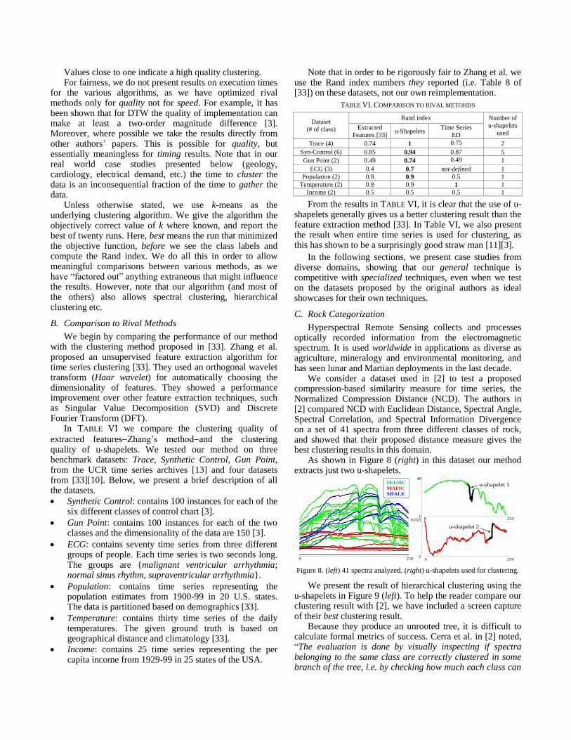
As shown in Figure 8 (right) in this dataset our method extracts just two u-shapelets.

Figure 8. (left) 41 spectra analyzed. (right) u-shapelets used for clustering.

We present the result of hierarchical clustering using the u-shapelets in Figure 9 (left). To help the reader compare our clustering result with [2], we have included a screen capture of their best clustering result.

Because they produce an unrooted tree, it is difficult to calculate formal metrics of success. Cerra et al. in [2] noted, “The evaluation is done by visually inspecting if spectra belonging to the same class are correctly clustered in some branch of the tree, i.e. by checking how much each class can

FELSIC

MAFIC

SHALE

0 2500

40

0

0.025

u-shapelet 2

u-shapelet 1

0 2500 250

be isolated by ‘cutting’ the tree at convenient points.” If we cut the tree of Figure 9 (right) at the points where we placed the pink lines, we find that the eleven nodes encircled are not clustered correctly. Whereas if we use the two shapelets only three Felsic and two Mafic rocks are clustered incorrectly. This simple experiment suggests that our clustering method can be used to cluster spectral signatures and it outperforms a variety of methods tuned for this application domain.

Figure 9. Hierarchical clustering (left) using u-shapelets, (right) using NCD

(screenshot of Fig. 4 from [2]). All pink lines are annotations added by us.

D. Synthetic Dataset 1

While real datasets such as the one used in the last section are the most convincing demonstrations of our algorithm, in this section (and the next) we consider synthetic datasets created by other researchers. We do this to demonstrate two things. First, the u-shapelets returned by our algorithm can offer insight into the data, and second, our very general unsupervised approach is competitive even with approaches where researchers design an algorithm, design synthetic datasets to showcase it, and provide supervision (i.e. class labels to their algorithm).

We first consider a synthetic dataset consisting of ten examples from two classes of univariate sequences [28] (the small size we consider is to allow direct comparison to the original paper [28], as it happens we get perfect results over a wide ranges of data sizes). The first class is a sinusoidal signal while the second class is a rectangular signal, both of which are randomly embedded within segments of Gaussian noise. In Figure 10, we show two examples of sequences from each class. Because the time series are of different lengths, the Euclidean Distance is not defined here. DTW can be used, but as the authors [28] show, the presence of noise and the misalignment of sinusoidal and rectangular signals greatly degrade DTW’s performance.

In order to deal with the noise and the misalignment of signals, Shahriar et al. in [28] proposed an approach for sequence alignment based on canonical correlation analysis (CCA). Their method, Isotonic CCA (IsoCCA), generalizes DTW to cases where the alignment is accomplished on arbitrary subsequence segments, instead of on individual samples. They used a 1-NN classifier and the leave-one-out cross validation to classify the twenty signals and reported that the classification accuracy is 90% when using IsoCCA, and 60% when using DTW.

It is important to note that these results are for classification accuracy; that is to say, this method requires class labels during training time. In contrast, our clustering algorithm does not see class labels when it runs, and

evaluates the clusters using classification accuracy on holdout data after the clustering is complete.

Using our method, the sinusoid signal is extracted as the sole u-shapelet and by using that u-shapelet, we can get 100% classification accuracy. In Figure 10, we mark the sinusoid u-shapelet discovered with its nearest neighbors in three other randomly chosen time series in red/bold. The orderline illustrates the subsequence distances to the sinusoid u-shapelet. We can see from the orderline in Figure 10 that the Rand index will be one when we cluster the dataset using the subsequence distances of the sinusoid u-shapelet.

Figure 10. Two examples of sinusoidal signals and rectangular signals.

Sinusoid u-shapelet and its nearest neighbors in the signals are marked with

red. The orderline shows the subsequence distances of the u-shapelet.

To summarize, here we can beat a rival approach, on the

data created by the proposed authors, even though they

exploit class labels during training time, a luxury that we

deny our approach.

E. Synthetic Dataset 2

The attentive reader may wonder whether the superior performance of u-shapelets in the previous section was due to the fact that there is no intra class variability within the sinusoidal or rectangular signals. Fortunately, the datasets created in [7] allows us to test this. The dataset consists of four classes. All the time series are composed of embedded class signals and additional noise; however, the class signals have significant randomly generated variations in length and height. Moreover, the defining shapes of classes two and three are composed of the “sub-signal” shape of classes one and four. In Figure 11, we present two time series from each class of the dataset.

Figure 11. Sample Time series of Synthetic Dataset 2. Classes 1 and 2, and

classes 3 and 4 are confused by most clustering methods.

Hartmann et al., [7] shows that when they use their method on just class one and class four, they can get good results. However, their method performs poorly if required to consider all four classes. We applied our algorithm to the same set of permutations of classes as the original paper [7]. In all cases, the Rand index is much better than the original author’s results (modulo slight difference in how the results are reported [7]). For example, only one u-shapelet is used for the class-1 vs. class-4 variant, and the Rand index is perfect (equal to one); Figure 12 illustrates the u-shapelet and the corresponding orderline. The Rand index is also

Sinusoidal signal Rectangular signal

0 ∞Orderline

class 1 class 2 class 3 class 4

Screen Group

Oven/Cooker

Washing

Machine

Immersion

Heater

Dishwasher

Cold Group

Kettle

0 10024 hour

perfect when we consider the more difficult class 2 vs. class 3 variant, but our algorithm uses four shapelets in this case.

Figure 12. u-shapelet from class 1 and the corresponding orderline.

Note that, once again, we are comparing with an algorithm that was co-developed with a synthetic dataset designed to showcase the algorithms strength, and once again we easily beat the proposed algorithm.

Furthermore, the original authors solved the problem of supervised learning by using prototypes or subsequences of the data which they learned from the training data. In contrast, we are clustering time series using u-shapelets or without any prior knowledge about the dataset.

This experiment provides us with the perfect opportunity to clarify an important point. There is no strict relationship between the number of clusters k, and the number of u-shapelets required to create k clusters. In particular, our algorithm requires four shapelets to cluster class-2 and class-3 into the correct two clusters. To illustrate, we show all the u-shapelets extracted by our method in Figure 13, and show the change in the Rand index as we add seven u-shapelets one by one. The last two u-shapelets are just random noise, because by that stage of the extraction, all meaningful patterns have been discovered by our algorithm. Note that even though essentially random u-shapelets are extracted in the late stages of our algorithms run, they do not affect the clustering result, as shown by the blue curve in Figure 13.

Figure 13. All the u-shapelets from class-2 vs class-3 version of [7]. bottom

right) The blue curve shows Rand index relative to the ground truth, as we

add u-shapelets. The gray line shows the Rand index if the whole time series is used for clustering. The red curve shows the change in Rand index

with the addition of u-shapelets. This curve correctly predicts that four u-

shapelets is best for this problem

F. Clustering Household Devices:

In order to reduce carbon emissions, the UK government has planned to equip 27 million households with an intelligent metering system (cf. Figure 14) at a cost of approximately £10 billion. As a useful by-product, these devices allow individuals to observe their electricity consumption and decrease their carbon footprint. This project is supported by a Cambridge-based company, Green Energy Options (GEO), which has installed the monitoring devices in 187 homes across East Anglia and recorded the

usage of individual devices (cf. Figure 14 (left)) at 15 minute intervals for approximately a year.

Figure 14. (left) Examples of electricity usage profiles of a single day for

the seven devices considered (screen shot from [15]), (right) smart energy

management display system.

The clustering problem here is difficult because of the high intra-class variability. Different houses use different devices during different times of the day. Moreover, there is also variability among the power consumption of the devices depending on the brand, etc.

Bagnall et al., in [15] classifies household appliances using these electricity usage profiles. They derived a set of features (min, max, mean, skewness etc.) to classify the data. We used a subset of the dataset that contains 2,073 time series to test our clustering method. Each time series corresponds to the electric usage profile of a household item over 24 hours. If we use whole time series to cluster the dataset, the Rand index is 0.56, whereas by using the u-shapelets, we can achieve a Rand index of 0.86.

In Figure 15, we have shown some of the u-shapelets that also provides insight about the data. For example, domain experts tell us that the two spikes shown in the dishwasher class correspond to the rinse and clean cycles.

Figure 15. Sample u-shapelets used for clustering.

G. Clustering Non-Invasive Fetal ECG:

Automatic analysis of ECG signals is needed to improve diagnostic systems. For this experiment, we have collected non-invasive fetal electrocardiograms (ECGs) signals from PhysioNet [5], an online medical archive containing digital recordings of physiological signals. As we have mentioned before, most classification and clustering algorithms consider only single heartbeats. We have extracted signals which are 3,000 points long. Each signal contains multiple heartbeats. The signals are taken from a single subject during the 22

nd

and 38th weeks of pregnancy. The dataset contains 948 such

signals. As the reader can see from Figure 16, the signals are not aligned perfectly. As a result, when we use entire time series for clustering the Rand index is 0.63 which is close to random. However using the u-shapelets we achieve a Rand index of 0.99.

Figure 16. The misalignment between ECG signals (indcated by the gray hatch lines)

recorded during (left) 22nd week and (right) 38th week of pregnancy.

u-shapelet

∞0

subsequence distances

of other class

orderline

1 2 3 4 5 6 70

0.5

1

u-shapelet 7

u-shapelet 6

u-shapelet 3

u-hapelet 5u-shapelet 4

u-shapelet 2u-shapelet1

number of u-shapelets

Ran

d In

dex

change in Rand index is 0

and we stop adding u-shapelets

Rand index using time series

Rand index using 4 u-shapelets is 1

0 1000

600

Dishwasher

0 100

0

400

Oven/Cooker

0 1000

400

Washing Machine

0 1000

400

Dishwasher

0 1000

600

Washing Machine

0 1000

300

Oven/Cooker

0 0 30003000

t min

t +1min

Figure 17 presents the first u-shapelet and the corresponding orderline. Note that for visual clarity, we plotted subsequence distances for ECG signals of week 22 and week 38 in two different lines with two different colors. When we asked cardiologist, Dr. (redacted for blind review) about the u-shapelets, he suggested that it corresponds to the p-wave of the ECG signal, known to change as a function of the developing fetus’s changing heart morphology.

Figure 17. (left) The 1st u-shapelet (red/bold) and (right) its corresponding orderline.

VI. CONCLUSION AND FUTURE WORK

We have illustrated the importance of ignoring some data in order to cluster time series in real world applications under realistic settings. We have introduced unsupervised shapelets and showed their utility. Our method can select representative u-shapelets from a time series without any human intervention. We have shown the utility of our algorithm in rock categorization, clustering household devices based on their electricity usage profiles, and clustering ECG signals. Our very general method is competitive even when tested it on synthetic datasets generated by other authors to explain their own proposed algorithms. We have also tested our method with statistical based clustering, the most obvious strawman.

Currently, we search for one u-shapelet (at at time) that can separate subsets of a dataset. However, one can imagine that in some circumstances, a linear combination of u-shapelets may be better able to create a single split. We leave this as a direction for future research.

Finally, we have not explained why u-shapelets work so well, given their unintuitive “chicken-and-egg” paradoxical nature noted above. We have definite ideas about this, supported by initial tentative empirical evidence. However, we will defer a detailed discussion about this topic until we can do it justice.

ACKNOWLEDGEMENT

This work was funded by NSF IIS - 1161997.

REFERENCES

[1] D. J. Berndt and J. Clifford, “Using Dynamic Time Warping to find

Patterns in Time Series,” AAAI-94 Workshop on Knowledge

Discovery in Databases, pp. 229–248. [2] D. Cerra, J. Bieniarz, J. Avbelj, P. Reinartz, and R. Mueller,

“Compression-based unsupervised clustering of spectral signatures,”

Hyperspectral Image and Signal Processing: Evolution in Remote Sensing (WHISPERS 2011).

[3] H. Ding, G. Trajcevski, P. Scheuermann, X. Wang, and E. Keogh, “Querying and mining of time series data: experimental comparison of

representations and distance measures,” PVLDB 2008, pp 1542–52.

[4] M. Garilov, D. Anguelov, P. Indyk, and R. Motwani, “Mining the stock market: Which measure is best?” Proc. ACM KDD 2000.

[5] A. L. Goldberger, et al. PhysioBank, PhysioToolkit, and PhysioNet: Circulation. Discovery vol. 101 (1997).

[6] M. Halkidi, Y. Batistakis, and M. Vazirgiannis, “On clustering

validation techniques,” Journal of Intelligent Information Systems.

[7] B. Hartmann, I. Schwab, and N. Link, “Prototype optimization for

temporarily and spatially distorted Time Series,” AAAI Spring Symposium Series (SSS 2010), pp. 15–20.

[8] S. Hirano and S. Tsumoto, “Cluster analysis of Time-series Medical

data based on the Trajectory representation and multiscale comparison techniques,” Proc. ICDM 2006.

[9] D. Jiang, C. Tang, and A. Zhang, “Cluster analysis for gene

expression data: A survey,” IEEE Trans. On Knowledge and data engineering (2004), vol. 16, no. 11, pp. 1370–1386.

[10] K. Kalpakis, D. Gada, and V. Puttagunta, “Distance measures for

effective clustering of ARIMA Time-Series,” ICDM 2001. [11] E. Keogh, S. Kasetty “On the need for Time Series Data Mining

Benchmarks: a survey and empirical demonstration,” Proc. ACM

KDD 2002, pp. 102–111. [12] E. Keogh, J. Lin and W. Truppel, “Clustering of Time Series

Subsequences is meaningless: implications for past and future

research,” Proc. IEEE ICDM 2003, pp. 115–122. [13] E. Keogh, Q. Zhu, B. Hu, Y. Hao, X. Xi, L. Wei, and C. A.

Ratanamahatana, The UCR Time Series Classification/Clustering

Homepage: www.cs.ucr.edu/~eamonn/time_series_data/

[14] T.W. Liao, “Clustering of time series data—a survey,” Pattern

Recognition, vol. 38, 2005, pp. 1857–1874.

[15] J. Lines, A. Bagnall, P. C. Smith, and S. Anderson, “Classification of Household Devices by Electricity Usage Profiles,” IDEAL 2011,

LNCS vol. 6936.

[16] J. Lines, L. Davis, J. Hills, and A. Bagnall, “A Shapelet filter for time series classification,” ACM SIGKDD 2012, in press.

[17] J. Lin, R. Khade, and Y. Li, 2012. “Rotation-invariant similarity in time series using Bag-of-Patterns representation,” Journal of

Intelligent Information Systems, 2012, in press.

[18] R. Kosala and H. Blockeel, “Web Mining Research: A Survey,” ACM SIGKDD, 2000.

[19] F. Möerchen, “Time series feature extraction for data mining using

dwt and dft,” Technical Report No. 33, 2003. [20] K. Muata, “Post-pruning in decision tree induction using multiple

performance measures,” Computers and Operations Research, 2007.

[21] A. Mueen, E. Keogh, and N. Young, “Logical-Shapelets: an expressive primitive for Time Series classification,” Proc. ACM

SIGKDD, 2011, pp. 1154–1162.

[22] A. Mueen, S. Nath, and J. Liu, “Fast approximate correlation for massive Time-Series data,” SIGMOD 2010, pp. 171–182.

[23] T. Rakthanmanon, E. Keogh, S. Lonardi, and S. Evans, “Time Series

Epenthesis: Clustering Time Series Streams requires ignoring some Data,” Proc. IEEE ICDM 2011.

[24] W. M. Rand, “Objective criteria for the evaluation of clustering

methods,” Journal of the American Statistical Association (1971). [25] C. A. Ratanamahatna and E. Keogh, “Making Time-series

classification more accurate using learned constraints,” Proc. SIAM

International Conference on Data Mining (SDM 2004). [26] E. J. Ruiz, V. Hristidis, C. Castillo, and A. Gionis, “Correlating

Financial Time Series with Micro-Blogging activity,” WSDM 2012.

[27] G. Salton, A. Wong, and C. S. Yang, “A vector space model for automatic indexing,” Commun. ACM (1975) vol. 19, pp. 613–620.

[28] S. Shariat and V. Pavlovic, “Isotonic CCA for sequence alignment

and activity recognition,” Proc. IEEE International Conference on Computer Vision (ICCV 2011), pp. 2572–2578.

[29] X. Wang, K. Smith, and R. Hyndman, “Characteristic-based

clustering for time series data,” DMKD, vol. 13, 2006, pp. 335–364.

[30] Webpage of our paper: https://sites.google.com/site/icdmclusteringts/, password: ICDM2012.

[31] Z. Xing, J. Pei, P. Yu, and K. Wang, “Extracting interpretable

features for early classification on time series,” Proc. SDM 2011. [32] L. Ye and E. Keogh, “Time Series Shapelets: a new primitive for

Data Mining,” Proc. ACM SIGKDD, 2009, pp. 947–956.

[33] H. Zhang, T. B. Ho, Y. Zhang, and M. S. Lin, “Unsupervised Feature Extraction for Time Series Clustering using Orthogonal Wavelet

Transform,” Journal on Informatics, vol. 30, Sep 2005, pp. 305–319.

[34] M. Zhang and A. A. Sawchuk, “Motion Primitive-Based Human Activity Recognition Using a Bag-of-Features Approach,” ACM

SIGHIT International Health Informatics Symp. (IHI 2012), pp. 1-10.

0 3000

0

22 week dtƟ

orderline

38 week

p-wave