University of Florida CISE department Gator Engineering

Clustering Part 4

Dr. Sanjay Ranka Professor

Computer and Information Science and Engineering University of Florida, Gainesville

University of Florida CISE department Gator Engineering

Data Mining Sanjay Ranka Spring 2011

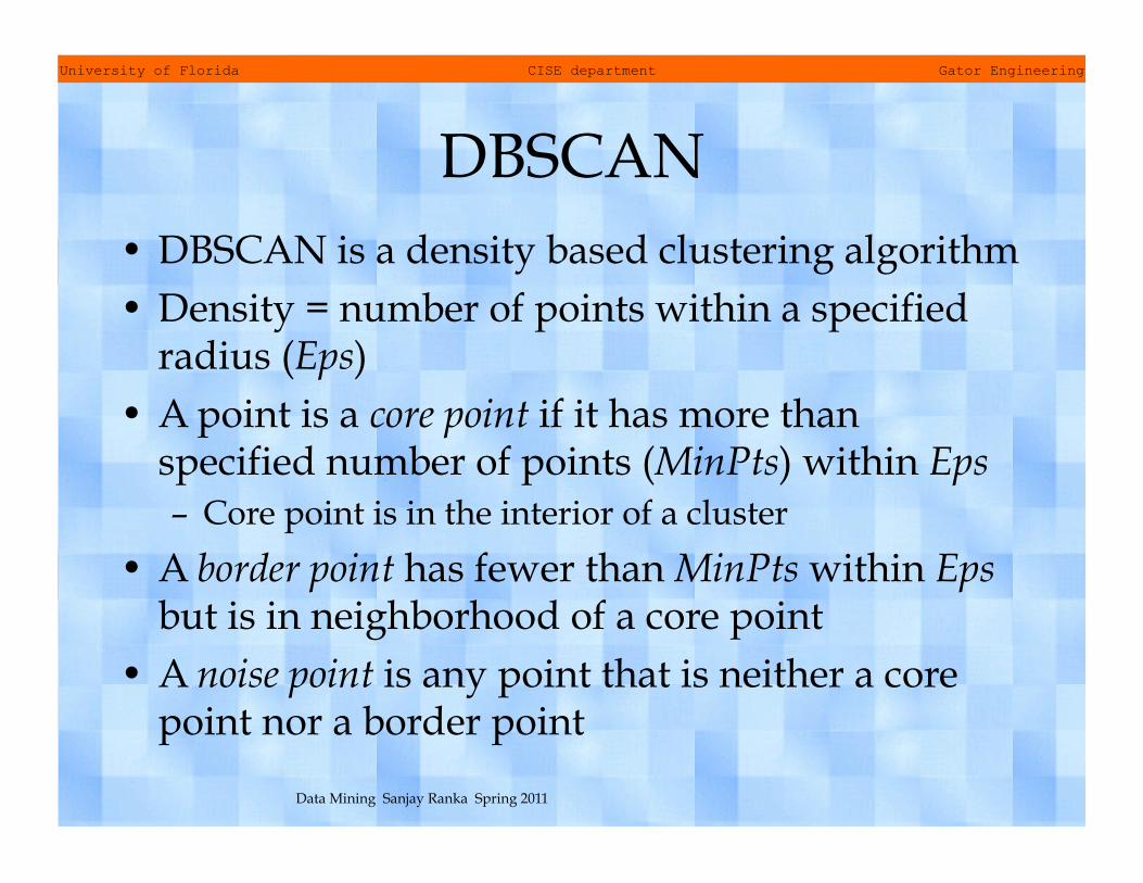
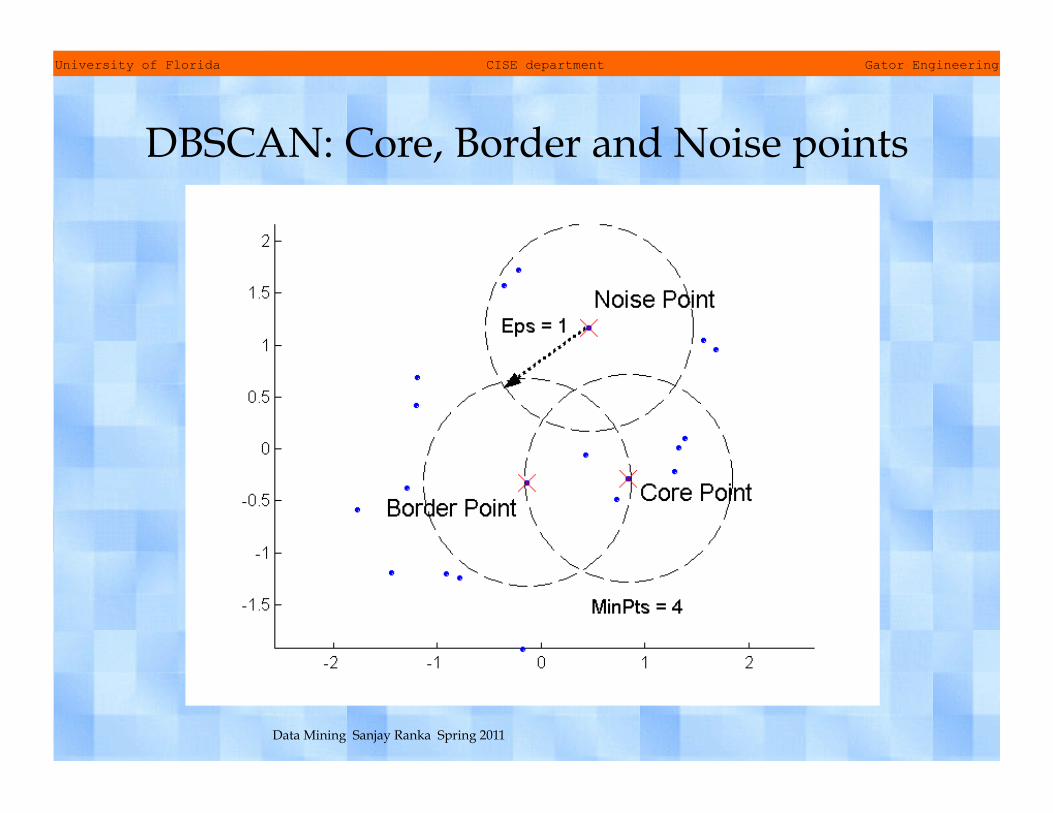
DBSCAN • DBSCAN is a density based clustering algorithm • Density = number of points within a specified

radius (Eps) • A point is a core point if it has more than

specified number of points (MinPts) within Eps – Core point is in the interior of a cluster

• A border point has fewer than MinPts within Eps but is in neighborhood of a core point

• A noise point is any point that is neither a core point nor a border point

University of Florida CISE department Gator Engineering

Data Mining Sanjay Ranka Spring 2011

DBSCAN: Core, Border and Noise points

University of Florida CISE department Gator Engineering

Data Mining Sanjay Ranka Spring 2011

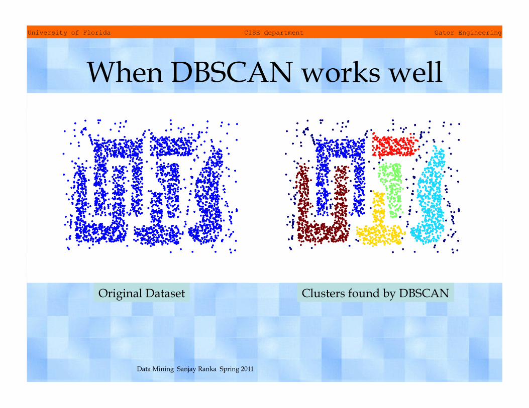
When DBSCAN works well

Original Dataset Clusters found by DBSCAN

University of Florida CISE department Gator Engineering

Data Mining Sanjay Ranka Spring 2011

DBSCAN: Core, Border and Noise points

Original Points Eps = 10, Minpts = 4 Point types:

Core Border Noise

University of Florida CISE department Gator Engineering

Data Mining Sanjay Ranka Spring 2011

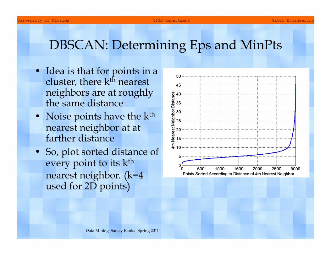
DBSCAN: Determining Eps and MinPts

•  Idea is that for points in a cluster, there kth nearest neighbors are at roughly the same distance

•  Noise points have the kth nearest neighbor at at farther distance

•  So, plot sorted distance of every point to its kth nearest neighbor. (k=4 used for 2D points)

University of Florida CISE department Gator Engineering

Data Mining Sanjay Ranka Spring 2011

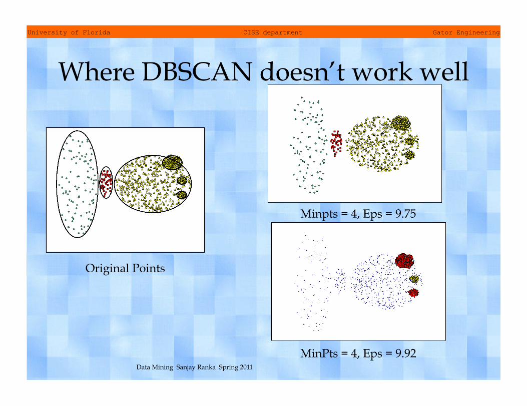
Where DBSCAN doesn’t work well

Original Points

MinPts = 4, Eps = 9.92

Minpts = 4, Eps = 9.75

University of Florida CISE department Gator Engineering

Data Mining Sanjay Ranka Spring 2011

DENCLUE • DENsity CLUstEring is a density clustering

approach that models the overall density of a set of points as the sum of influence functions associated with each point

• DENCLUE is based on kernel density estimation. The goal of kernel density estimation is to describe the distribution of data by a function

• For kernel density estimation, the contribution of each point to the overall density function is expressed by an influence (kernel) function. The overall density is then merely the sum of the influence functions associated with each point

University of Florida CISE department Gator Engineering

Data Mining Sanjay Ranka Spring 2011

DENCLUE • The resulting overall density functions will have

local peaks, i.e. local density maxima, and these local peaks can be used to define clusters – For each point, a hill climbing algorithm finds the

nearest peak associated with that point, and set of all data points associated with a peak form a cluster

– However, if the density at a local peak is too low, then the points in the associated cluster are labeled as noise and discarded

–  Similarly, if two peaks are connected by a path of data points, and the density at each point on the path is above a minimum density threshold ξ, then the clusters associated with these two peaks are merged

University of Florida CISE department Gator Engineering

Data Mining Sanjay Ranka Spring 2011

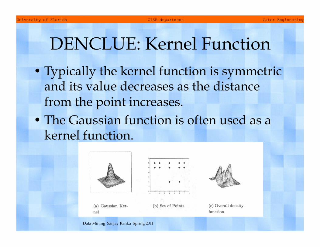
DENCLUE: Kernel Function • Typically the kernel function is symmetric

and its value decreases as the distance from the point increases.

• The Gaussian function is often used as a kernel function.

University of Florida CISE department Gator Engineering

Data Mining Sanjay Ranka Spring 2011

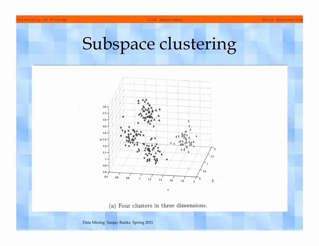
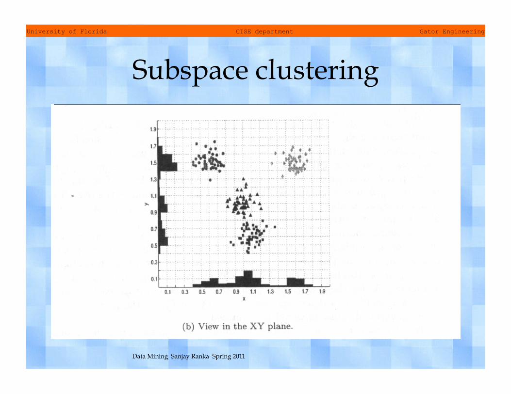
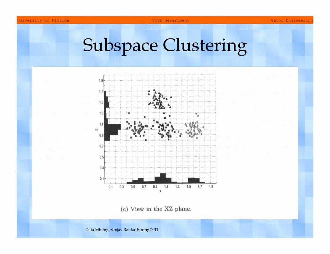
Subspace clustering • Instead of using all the attributes

(features) of a dataset, if we consider only subset of the features (subspace of the data), then the clusters that we find can be quite different from one subspace to another

• The clusters we find depend on the subset of the attributes that we consider

University of Florida CISE department Gator Engineering

Data Mining Sanjay Ranka Spring 2011

Subspace clustering

University of Florida CISE department Gator Engineering

Data Mining Sanjay Ranka Spring 2011

Subspace clustering

University of Florida CISE department Gator Engineering

Data Mining Sanjay Ranka Spring 2011

Subspace Clustering

University of Florida CISE department Gator Engineering

Data Mining Sanjay Ranka Spring 2011

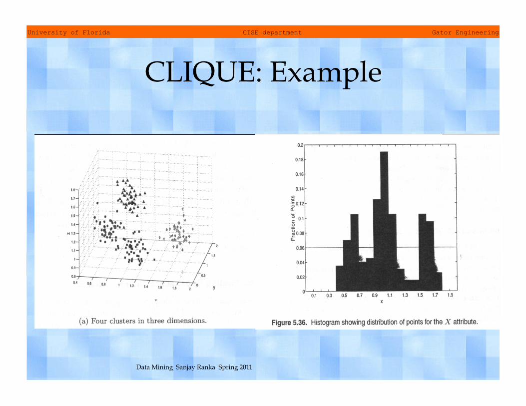
CLIQUE • CLIQUE is a grid based clustering algorithm • CLIQUE splits each dimension (attribute) in to a

fixed number (ξ) of equal length intervals. This partitions the data space in to rectangular units of equal volume

• We can measure the density of each unit by the fraction of points it contains

• A unit is considered dense if its density > user specified threshold τ

• A cluster is a group of contiguous (touching) dense units

University of Florida CISE department Gator Engineering

Data Mining Sanjay Ranka Spring 2011

CLIQUE: Example

University of Florida CISE department Gator Engineering

Data Mining Sanjay Ranka Spring 2011

CLIQUE • CLIQUE starts by finding all the dense areas in

the one dimensional spaces associated with each attribute

• Then it generates the set of two dimensional cells that might possibly be dense by looking at pairs of dense one dimensional cells

• In general, CLIQUE generates the possible set of k-dimensional cells that might possibly be dense by looking at dense (k-1)-dimensional cells. This is similar to APRIORI algorithm for finding frequent item sets

• It then finds clusters finds clusters by taking union of all adjacent high density cells

University of Florida CISE department Gator Engineering

Data Mining Sanjay Ranka Spring 2011

MAFIA • Merging of Adaptive Finite Intervals (And

more than a CLIQUE) • MAFIA is a modification of CLIQUE that

runs faster and finds better quality clusters. There is also pMAFIA which is a parallel version of MAFIA

• The main modification over CLIQUE is the use of an adaptive grid

University of Florida CISE department Gator Engineering

Data Mining Sanjay Ranka Spring 2011

MAFIA • Initially each dimension is partitioned into

a large number of intervals. A histogram is generated that shows the number of data points in each interval

• Groups of adjacent intervals are grouped in to windows, and the maximum number of points in the window’s intervals becomes the value associated with the window

University of Florida CISE department Gator Engineering

Data Mining Sanjay Ranka Spring 2011

MAFIA • Adjacent windows are grouped together if

the values of the two windows are close • As a special case, if all windows are

combined into one window, the dimensions is partitioned in to a fixed number of cells and the threshold for being considered a dense unit is increased for that dimension

University of Florida CISE department Gator Engineering

Data Mining Sanjay Ranka Spring 2011

Limitations of CLIQUE and MAFIA

• Time complexity is exponential in the number of dimensions

• Will have difficulty if “too many” dense units are generated at lower stages

• May fail if clusters are of widely differing densities, since the threshold is fixed

• Determining the appropriate τ and ξ for a variety of data sets can be challenging

• It is not typically possible to find all clusters using the same threshold

University of Florida CISE department Gator Engineering

Data Mining Sanjay Ranka Spring 2011

Clustering Scalability for Large Datasets

• One very common solution is sampling, but the sampling could miss small clusters. – Data is sometimes not organized to make

valid sampling easy or efficient.

• Another approach is to compress the data or portions of the data. – Any such approach must ensure that not too

much information is lost. (Scaling Clustering Algorithms to Large Databases, Bradley, Fayyad and Reina.)

University of Florida CISE department Gator Engineering

Data Mining Sanjay Ranka Spring 2011

Scalable Clustering: BIRCH • BIRCH (Balanced and Iterative Reducing

and Clustering using Hierarchies) – BIRCH can efficiently cluster data with a

single pass and can improve that clustering in additional passes.

– Can work with a number of different distance metrics.

– BIRCH can also deal effectively with outliers.

University of Florida CISE department Gator Engineering

Data Mining Sanjay Ranka Spring 2011

Scaleable Clustering: BIRCH • BIRCH is based on the notion of a

clustering feature (CF) and a CF tree. • A cluster of data points (vectors) can be

represented by a triplet of numbers – (N, LS, SS) – N is the number of points in the cluster – LS is the linear sum of the points –  SS is the sum of squares of the points.

• Points are processed incrementally. – Each point is placed in the leaf node corresponding to

the “closest” cluster (CF). – Clusters (CFs) are updated.

University of Florida CISE department Gator Engineering

Data Mining Sanjay Ranka Spring 2011

Scaleable Clustering: BIRCH • Basic steps of BIRCH

– Load the data into memory by creating a CF tree that “summarizes” the data.

– Perform global clustering. • Produces a better clustering than the initial step. • An agglomerative, hierarchical technique was selected.

– Redistribute the data points using the centroids of clusters discovered in the global clustering phase, and thus, discover a new (and hopefully better) set of clusters.

University of Florida CISE department Gator Engineering

Data Mining Sanjay Ranka Spring 2011

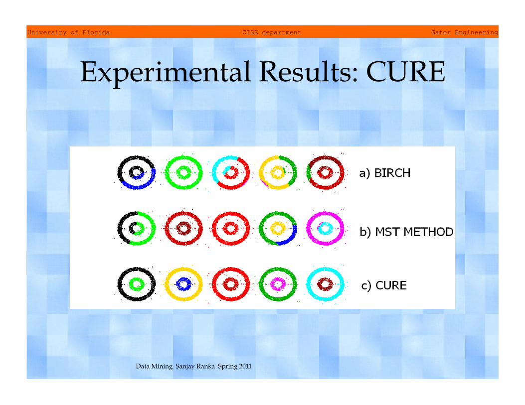
Scaleable Clustering: CURE •  Clustering Using Representatives •  Uses a number of points to represent a cluster •  Representative points are found by selecting a constant

number of points from a cluster and then “shrinking” them toward the center of the cluster

•  Cluster similarity is the similarity of the closest pair of representative points from different clusters

•  Shrinking representative points toward the center helps avoid problems with noise and outliers

•  CURE is better able to handle clusters of arbitrary shapes and sizes

University of Florida CISE department Gator Engineering

Data Mining Sanjay Ranka Spring 2011

Experimental results: CURE

University of Florida CISE department Gator Engineering

Data Mining Sanjay Ranka Spring 2011

Experimental Results: CURE

University of Florida CISE department Gator Engineering

Data Mining Sanjay Ranka Spring 2011

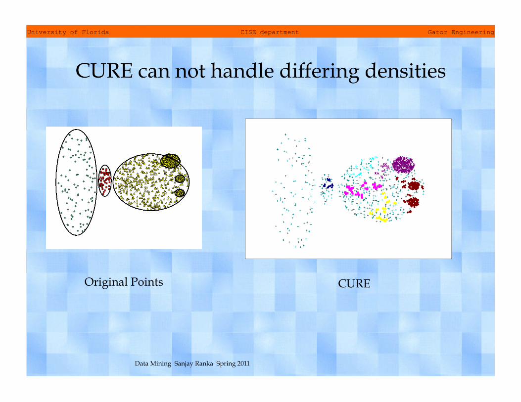
CURE can not handle differing densities

Original Points CURE

University of Florida CISE department Gator Engineering

Data Mining Sanjay Ranka Spring 2011

Graph Based Clustering • Graph-Based clustering uses the proximity

graph –  Start with the proximity matrix – Consider each point as a node in a graph – Each edge between two nodes has a weight which is

the proximity between the two points –  Initially the proximity graph is fully connected – MIN (single-link) and MAX (complete-link) can be

viewed as starting with this graph

• In the most simple case, clusters are connected components in the graph

University of Florida CISE department Gator Engineering

Data Mining Sanjay Ranka Spring 2011

Graph Based Clustering: Sparsification

• The amount of data that needs to be processed is drastically reduced – Sparsification can eliminate more than 99%

of the entries in a similarity matrix – The amount of time required to cluster the

data is drastically reduced – The size of the problems that can be

handled is increased

University of Florida CISE department Gator Engineering

Data Mining Sanjay Ranka Spring 2011

Sparsification • Clustering may work better

–  Sparsification techniques keep the connections to the most similar (nearest) neighbors of a point while breaking the connections to less similar points.

– The nearest neighbors of a point tend to belong to the same class as the point itself.

– This reduces the impact of noise and outliers and sharpens the distinction between clusters.

• Sparsification facilitates the use of graph partitioning algorithms (or algorithms based on graph partitioning algorithms. – Chameleon and Hypergraph-based Clustering

University of Florida CISE department Gator Engineering

Data Mining Sanjay Ranka Spring 2011

Sparsification

University of Florida CISE department Gator Engineering

Data Mining Sanjay Ranka Spring 2011

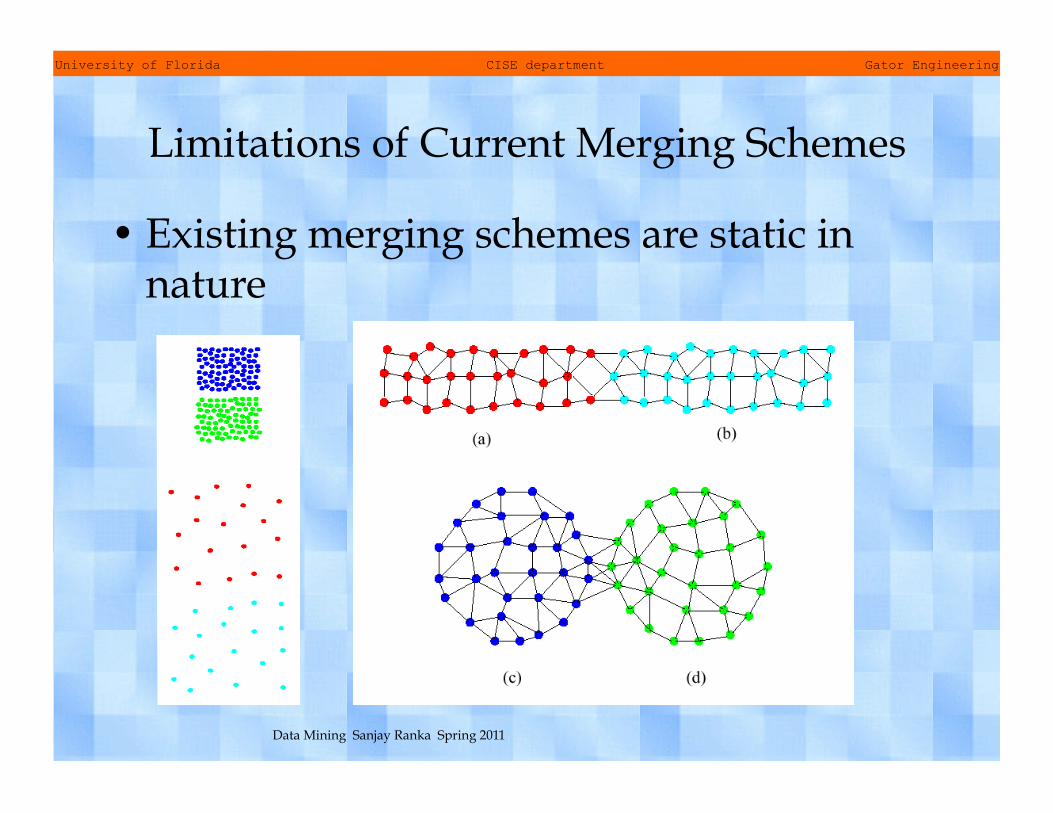
Limitations of Current Merging Schemes

• Existing merging schemes are static in nature

University of Florida CISE department Gator Engineering

Data Mining Sanjay Ranka Spring 2011

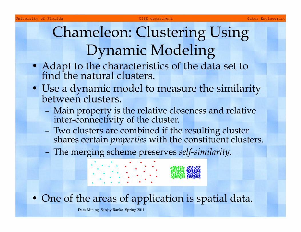
Chameleon: Clustering Using Dynamic Modeling

• Adapt to the characteristics of the data set to find the natural clusters.

• Use a dynamic model to measure the similarity between clusters. – Main property is the relative closeness and relative

inter-connectivity of the cluster. – Two clusters are combined if the resulting cluster

shares certain properties with the constituent clusters. – The merging scheme preserves self-similarity.

• One of the areas of application is spatial data.

University of Florida CISE department Gator Engineering

Data Mining Sanjay Ranka Spring 2011

Characteristics of Spatial Datasets •  Clusters are defined as densely

populated regions of the space •  Clusters have arbitrary shapes,

orientation, and non-uniform sizes

•  Difference in densities across clusters and variation in density within clusters

•  Existence of special artifacts (streaks) and noise

•  The clustering algorithm must address the above characteristics and also require minimal supervision

University of Florida CISE department Gator Engineering

Data Mining Sanjay Ranka Spring 2011

Chameleon • Preprocessing Step: Represent the Data by a

Graph –  Given a set of points, we construct the k-nearest-

neighbor (k-NN) graph to capture the relationship between a point and its k nearest neighbors.

• Phase 1: Use a multilevel graph partitioning algorithm on the graph to find a large number of clusters of well-connected vertices. – Each cluster should contain mostly points from one

“true” cluster, i.e., is a sub-cluster of a “real” cluster. – Graph algorithms take into account global structure.

University of Florida CISE department Gator Engineering

Data Mining Sanjay Ranka Spring 2011

Chameleon • Phase 2: Use Hierarchical Agglomerative

Clustering to merge sub-clusters. – Two clusters are combined if the resulting

cluster shares certain properties with the constituent clusters.

– Two key properties are used to model cluster similarity:

• Relative Interconnectivity: Absolute interconnectivity of two clusters normalized by the internal connectivity of the clusters.

• Relative Closeness: Absolute closeness of two clusters normalized by the internal closeness of the clusters.

University of Florida CISE department Gator Engineering

Data Mining Sanjay Ranka Spring 2011

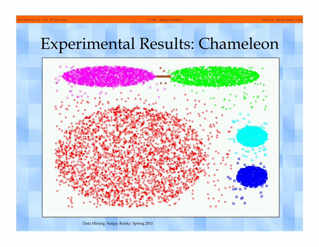
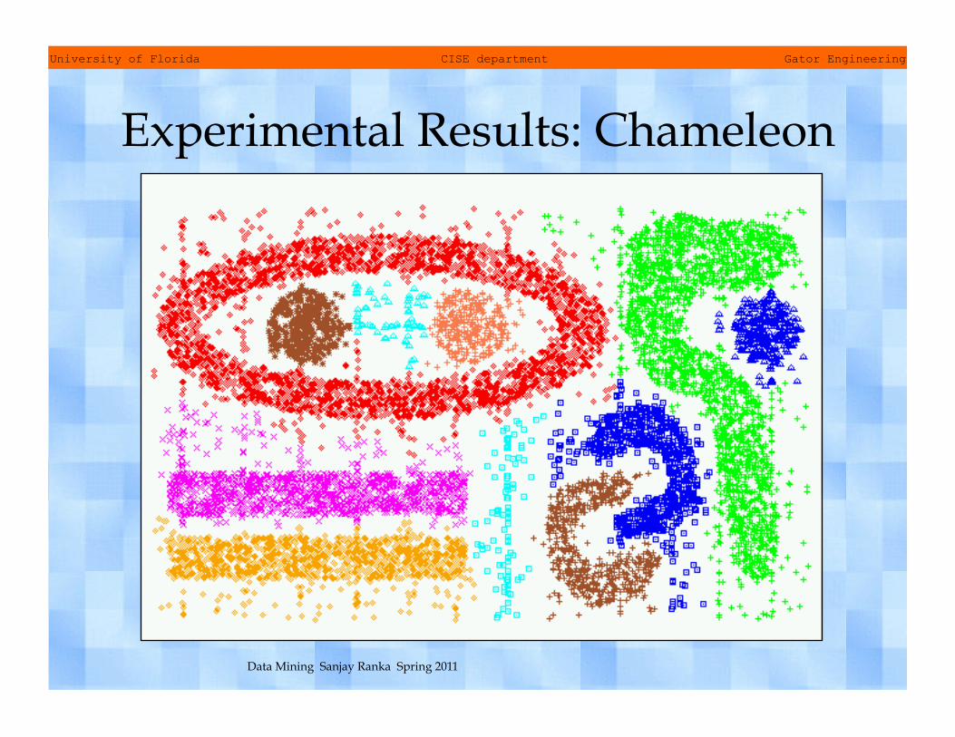
Experimental Results: Chameleon

University of Florida CISE department Gator Engineering

Data Mining Sanjay Ranka Spring 2011

Experimental Results: Chameleon

University of Florida CISE department Gator Engineering

Data Mining Sanjay Ranka Spring 2011

Experimental Results: CURE (10 clusters)

University of Florida CISE department Gator Engineering

Data Mining Sanjay Ranka Spring 2011

Experimental Results: CURE (15 clusters)

University of Florida CISE department Gator Engineering

Data Mining Sanjay Ranka Spring 2011

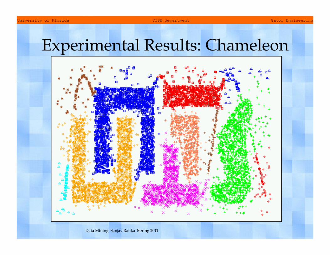
Experimental Results: Chameleon

University of Florida CISE department Gator Engineering

Data Mining Sanjay Ranka Spring 2011

Experimental Results: CURE (9 clusters)

University of Florida CISE department Gator Engineering

Data Mining Sanjay Ranka Spring 2011

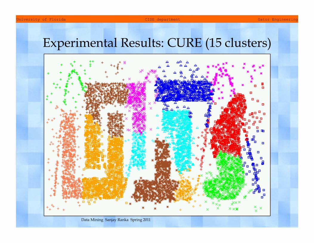
Experimental Results: CURE (15 clusters)