Directed Research, presented as part of the requirements for the

Award of the Masters Degree in Finance of NOVA School of Business and Economics.

CLUSTER ANALYSIS AND SEGMENTATION

OF

GLOBAL M&A TRANSACTIONS

RICARDO MOUTINHO TEIXEIRA

Masters Student Number 390

Direct Research was carried out under the supervision of Professor José Neves de Almeida,

Nova School of Business and Economics, Lisbon

January 2013

Abstract: The present thesis is the analysis a dataset of mergers and acquisitions (M&A) through a segmentation

process by cluster analysis, to better understand combined explanatory variables and characteristics of global M&A

transactions. Past researched has strongly focused on (A) whether or not M&A creates wealth for investors or (B)

which factors and variables help explain value this wealth (des)creation. The present thesis is rather an attempt to

reach a third leg of research which is that, by segmenting and understanding these “natural” groupings we may

develop a richer understanding of this form of corporate transactions. The paper comprises a study-event dataset

from global completed M&A since 1994 with high disclosure filters, a factor analysis that selected 7 out of 13

variables from previous literature review, preceded by a the cluster analysis for variable selection. The end result

indicated a connection between several explanatory variables and the formation of clusters with economical

meaning. Six clusters were formed under a two-step clustering process. The paper has three relevant highlights: (1)

the application of cluster analysis in a M&A setting; (2) the selection of surrogate variables from the factor analysis,

providing better economic representation and (3) a clustering method that automatically captures the natural

grouping the dataset.

Keywords: Mergers and Acquisitions (M&A); Value Creation; Factor Analysis (FA); Cluster Analysis (CA);

Segmentation.

Dedicated to Mom and Dad, for your constant love and support.

You have held my hand in difficult times and believed in me throughout my journey.

Thank you.

3

1. Introduction

As with the auto industry, where one cannot properly assess the overall sales or profitability of

a car manufacturer’s – in our case value creation from M&A transactions – without

understanding that, for example, that sedan or compact vehicles have product but also have

different target audiences, market dynamics and cost drivers.

That concept gave the paper its study hypothesis: can a segmentation process be done for M&A

transactions due to its different characteristics, actors and large complexity? In order to apply

the same idea, the present thesis contains the review of the right variables and metric that

measures value creation, to then later adequately segment and interpret the results from the

Cluster Analysis (CA). Methodologically, an event-study dataset is constructed from the

Bloomberg M&A database, the Factor Analysis (FA) selects the variables for the clustering

process and finally, the two-step CA is put in places based on a distance measure log-likelihood

and a Schwarz's Bayesian Criterion (BIC) for clustering criterion. Following the Literature

Review and Methodology, readers will find a section for commentary of the results, managerial

implications and overall summary under the Conclusion.

The prime research objective of the paper in the attempt to properly classify M&A transaction

is to bring to research areas of M&A and Value Creation a new paradigm and discussion level

for both practitioners and research community.

4

2. Literature Review

The literature review for the present thesis undergoes the following order: (1) understand the

selection of an event-study dataset, as well as its timeframe, metric of value creation and

variables and (2) comment on research for the FA and CA which will detailed further on the

Methodology section.

Robert F. Bruner (Bruner, 2002) found that out of that there are four research approaches

employed to measure M&A value creation: event studies, accounting studies, surveys and

clinical studies, of which event studies clearly dominated literature. Event studies examine

abnormal returns for within a defined time horizon around the transaction (normally centered

around the announcement date). From his paper came the decision to pursue a dataset based on

event studies, allowing for more a representative sample and leveled playfield across all

transactions. However, accounting studies require access to accounting statements and a

common legal framework and accounting standards. Furthermore, survey to executives and

clinical studies are specific to a small set of cases (firms and executives), which may bring

some bias and unrepresentative view, especially when trying to grasp a broad overview of

M&A transactions globally. His paper proved additionally important in the Methodology

section as it as studies what it means for M&A to “pay” in review of 130 studies from 1971 to

2001.

The paper from McKinsey (Cyriac, Koller, & Thomsen, 2012) provides with the argument for

using Excess Total Return to Shareholders as the adequate metric for measuring value that

mergers and acquisitions create. Still, two other metrics were considered: (1) comparison of

share prices before and after a deal is announced and (2) accounting metrics, example of

Economic Profit. The first alternative, takes into account short-term investor reactions as an

indicator, with the sole benefit of providing a measure of value unimpaired by other events due

to the reduced term of the analysis, such as subsequent acquisitions or other corporate events

5

post-acquisition. This metric however, relies on short-term market reaction to gauge value

creation not allowing investors to “digest” adequately the value of a transaction. This is a major

step in the research process, as not following this path implies not accepting as true the

Efficient Market Hypothesis (EMH). The big reason is that, if it is plausible to infer that a great

majority of transactions take a great deal of time and resources for corporations to analyze

before a decision is made, than why would it not take at least the same amount of time for the

investor community to assess such transaction before trading on the stock? Moreover, a short-

term measure does not give investors time enough to evaluate the success of the post-merger

process (Ikenberry, Lakoniskok, & Vermaelen, 1995). The second alternative would be through

an accounting measure such as Economic Profit. As justified above, it is hard to put in practice,

due to different accounting standards, legal framework and limited access to information. One

would need to obtain for instance the combined Net Operating Profit After Taxes (NOPAT)

from the deal, which would reduce substantially the sample. Moreover, Weighted Average Cost

of Capital (WACC) and the Economic Capital employed (K) are variables affected by attritions

such as the tax shield having a (likely) different and unknown target capital structure and new

cost of debt will exist after the deal. Therefore, in order to adequately measure Economic Profit

one would need to know the new cost of debt (kd), which unlike the cost of equity, that can

reflect changes in operational and financial leverage through leveraged beta, and have the target

capital structure that would arise from the transaction, in most cases it is neither attainable nor

is it scalable to such global M&A databases.

Asquith (1983) argues that measurement of wealth effects is insignificant around the

consummation date. Furthermore, in order to fully understand wealth effects to the bidder’s

shareholders, it becomes paramount to measure before and after effects of a deal around the

announcement date, where most of the abnormal returns are generated. Asquith gave us a clear

perspective on how important the timeframe was for an adequate analysis. The period of return

6

measurement defined for our study is one calendar year counting from the announcement date,

further explained in the Methodology.

Datta, Pinches and Narayannan (1992) found that the relevant factors that determine M&A

wealth creation are: regulatory changes, the number of bidders, the bidders approach (i.e.

merger or tender offer), the mode of payment (i.e. cash, stock) and the type or motive of

acquisition. Furthermore, the value chain, relationship and economic area of each M&A

transaction are significant for wealth creation (Hoang & Lapumnuaypon, 2007). Value chain

refers to: (1) vertical M&A, (2) horizontal M&A or (3) conglomerate M&A. Vertical M&A, is

defined with a transaction which combines client and supplier or client and seller. Firms

involved seek to reduce uncertainty and transaction costs by upstream and downstream linkages

in the value chain and to benefit from economies of scope (Chen & Findlay, 2003); In the case

of Horizontal M&A, both parties are competing firms in the same industry. In this case,

eliminating competition, economies scale, acquiring or accessing a certain capability or

technology is amongst the biggest are the biggest motives that justify this form of M&A.

Lastly, in the attempt of reduce and diversify risk companies might engage in Çonglomerate

M&A. Based on the findings of Megginson, Morgan and Nail (2004) “mergers that decrease

focus result in significant losses in relative shareholder wealth, operating performance, and firm

value over the three years following merger completion” as with mergers that preserve of

increase focus these “result in marginal improvements in long-term performance”. Supported

by the empirical evidence and references of the authors, it seemed rational to include the type

of M&A as a variable to be analyzed. The relationship refers to the nature as with the

transaction occurred, in simply termed “friendly” or “hostile”. A hostile bid occurs when an

unsolicited or uniformed occurs from the part of the bidder to the target company’s Board of

Directors. A friendly deal, is when a deal is pre-approved by the Board of Directors and each

7

other’s’ interests are met and both agree to the proposed deal (Datta, Pinches, & Narayanan,

1992).

Two other important papers provided further support for relevant explanatory variables in

M&A. The first paper is from KPMG’s Advisory team (Tiemann & Kelly, 2010) which

summarizes the key variables that are able to generate both higher and lower abnormal returns

through corporate M&A: (1) cash-only deals had higher returns than both stock-and-cash and

stock-only deals; (2) acquirers with lower P/E ratios completed more successful deals; (3) the

number of past deals pursued by an acquirer was relevant, or as commonly mentioned the

M&A experience was a significant factor; (4) the reason to pursue a deal did matter, that those

transactions that were motivated by increase financial strength were most successful, more than

those motivated by a desire to acquire IP or technology and the motivation to increase revenue

was the least successful; (5) the size of the acquirer, as measured by its market capitalization,

was not a statically significant element. The second paper is from McKinsey (Cyriac, Koller, &

Thomsen, 2012) were they analyze the world’s top 1000 nonbanking companies’ M&A

practices and find that (1) the size of the target acquired matters (market capitalization); (2)

number of deals per year each organization pursues. From these papers, which have in their

selves comprise great literature reviews and the experience of two important advisory teams,

we are able to later understand the kind of variables to capture from our dataset later.

8

3. Methodology

3.1 Event-study dataset

Having the right methodology was key to acquire and organize the dataset and, to be able to

achieve the present results. From the structure defined in the Introduction the Methodology is

broken down into (A) the preparation of the dataset so it can be prepared for a statistical study,

(B) detail of the value creation metric, timeframe and explanatory variables and ultimately, (C)

processes and methods for the FA and CA.

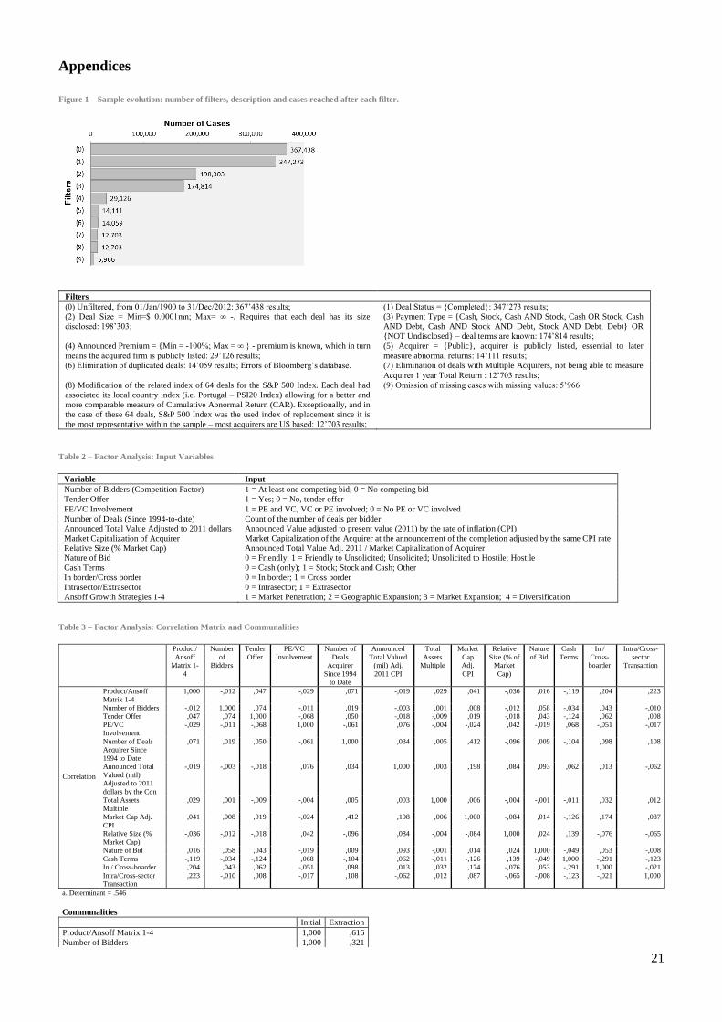
The selected sample comprises 5’966 transactions and was collected from Bloomberg’s M&A

database, with all filters based on information level and disclosure (Figure 1). The research

process starts with collecting and formatting data into to Excel, calculating and integrating

same relevant variables from there and later on preparing the dataset to be transposed IBM

SPSS 21.

“Factors Influencing Wealth Creation from Mergers and Acquisitions: A Meta-Analysis”

(Datta, Pinches, & Narayanan, 1992) was a great entry point to help organize the Bloomberg

M&A database. Not only did the authors review and summarize 41 studies on M&A wealth

effects, they described the select few factors that better explain wealth gains for bidding and

target shareholders involved and, that M&A studies were mainly driven by ‘targets’ and

`bidders’. Bidding firms are those that initiate the transaction and a target firm or asset is the

object of interest. Logically, this point defined that our sample and the variables to be analyzed

were transaction-based. Rather than organizing our date into a set of aggregate bidders’

transactions, a transaction-based sample was more meaningful and easier to measure. The

transactions listed in the Bloomberg M&A database was then ordered by announcement date.

In the dataset, an acquirer listed was already known to be the winning bidder in case of

competing bid process, since only completed transactions were listed. Information on

competition was limited as Bloomberg only listed whether or not a transaction was had a

9

competing bid, a mandatory offer or neither. Although mentioned as important by several

authors in our literature review, the mode of payment was not fully disclosed by Bloomberg.

We knew if a public transaction was financed solely with cash as it was mentioned. If any

exchange terms were disclosed we could only conclude that the specific transaction was not

fully financed with cash.

As described in the paper reviews both the results by the McKinsey & Co. paper (Cyriac,

Koller, & Thomsen, 2012) as well as the fit provided by Bruner (2002) with the event-study

research on M&A, Excess Total Return to Shareholders (TRS) is the metric used to gauge

value creation. For the purposes of the thesis the designation followed is Cumulative Abnormal

Return (CAR).

Equation 1 - Cumulative Abnormal Return (CAR)

∑

∑

Notes: Total Return to Shareholders captures capital appreciation from stock price changes, regular and special cash dividends as well as stock

buybacks. Since different stocks have different levels of political and country risks, a formula was created with the Bloomberg Microsoft Excel

plug-in to select the corresponding country index according to Bloomberg – e.g. if General Electric as an acquirer completed transaction,

Bloomberg would select S&P 500 as the index to measure total return from.

The timeframe for measuring CAR for each transaction is one year, the reason being to

minimize calendar distortions, seasonal effects and provide enough time for investors to act on

these corporate events. One year is the balance between an enough time for investors to

perceive value creation, while reducing seasonality effects by not having over one year,

reducing the number and effect of other corporate or strategic events. As explained before with

the CAR, this hypothesis is treated with care as it is not consistent with the EMH. Still,

reflecting carefully, if the EMH were to be in place, it would not make much sense to analyze

further than the one day period do it the immediate market reaction and yet authors (Ikenberry,

Lakoniskok, & Vermaelen, 1995) found that there is a slow investor reaction to share

10

repurchases (the simplest of the corporate events), implying average abnormal returns to be

made over time, evidence that is aligned with the paper and inconsistent with the EMH.

From the research papers the relevant explanatory M&A transaction variables we were not able

include in our analysis neither regulatory changes nor motives for a transaction. These were not

always disclosed or captured in the Bloomberg M&A database. The included variables for the

later FA are: (1) Number of Bidders (competing factor), whether there were any other bidding

offers competing for the deal before the deal was closed by the acquirer; (2) Tender Offer, a yes

or no variable that considers if there was any tender offer in place; (3) PE/VC involvement, a

binary variable that picks-up the records from Bloomberg both from Buy and Sell side and

records if there were any Private Equity or Venture capital firms involved; (4) Deal Experience,

from 1994 to the year-end of 2011, counts the number deals pursued from acquirers; (5)

Announced Total Value Adjusted to 2011 dollars is the announced transaction amounts where

each transaction is made comparable by the CPI1 providing a relative comparable between

transaction; (6) Total Assets Multiple; (7) Market Capitalization of the Acquirer, also adjusted

by the CPI; (8) Relative Size, the percentage of the deal amount to the acquirer’s market

capitalization at the announcement date, providing a measure of relative importance; (9) Nature

of the Bid, identified by Bloomberg from a range of Friendly to Hostile; (10) Cash Terms,

which if either the deal was fully financed with Cash or not; (11) if the transaction is

considered either In border or Cross border; (12) if it is considered Intrasector, within the same

sector, or Extrasector; (13) Ansoff’s Growth Strategies, where each transaction is classified

from one to four according to the type of transaction underdone.

1 Consumer Price Index (CPI) – due to the economic importance and relevant stake of the Unites States economy in global M&A and widely

used measure, the CPI is a good way to make comparable M&A transactions over time as it is a “measure of the average change over time in

the prices paid by urban consumers for a market basket of consumer goods and services.” (Bureau of Labor Statistics, 2010)

11

3.2 Factor Analysis (FA)

In the case of large sets of data, there tends to be are a large number of possible variables for

selection. If already disregarding meaningless variables, many others tend to be correlated and

must be reduced to a manageable level, allowing for a balanced and more sensible analysis later

on. Therefore, the method of FA is used primarily for data purposes. The objective of the FA is

to determine the level of information being explained amongst variables, later allowing us to

assess the number of variables to be included in the CA (Malhotra, 2009). Variables should be

ideally measured on a ratio or interval scale, although not always possible, especially in a

M&A transaction dataset. Therefore, the analysis was conducted with variables considered

great in the interest of explaining value creation as well as were situated in some sort on

interval or fluctuation band (i.e. EBITDA multiple – although continuous, it is standardized and

comparable across transactions). Dedicated literature (Malhotra, 2009) also indicates that one

should, on reasonable terms, have as a sample 4 to 5 times the number of variables to be

included. It should not be a problem, since there are limited variables (13) for evaluating a

database of 5’966 cases. The Kaiser-Meyer-Olkin (KMO) Measure of Sampling Adequacy, as

the name suggests, by testing whether the partial correlations among variables are small

validating a sample’s adequacy. If KMO statistic is large enough (>0.5) one may proceed with

the analysis without having concerns with the sample. In this case 0.571 was obtained, a large

enough figure to comply with the analysis, understandable due to the large dataset and the fact

that some of the variables are continuous (e.g. Market Capitalization Adj. CPI) rather than

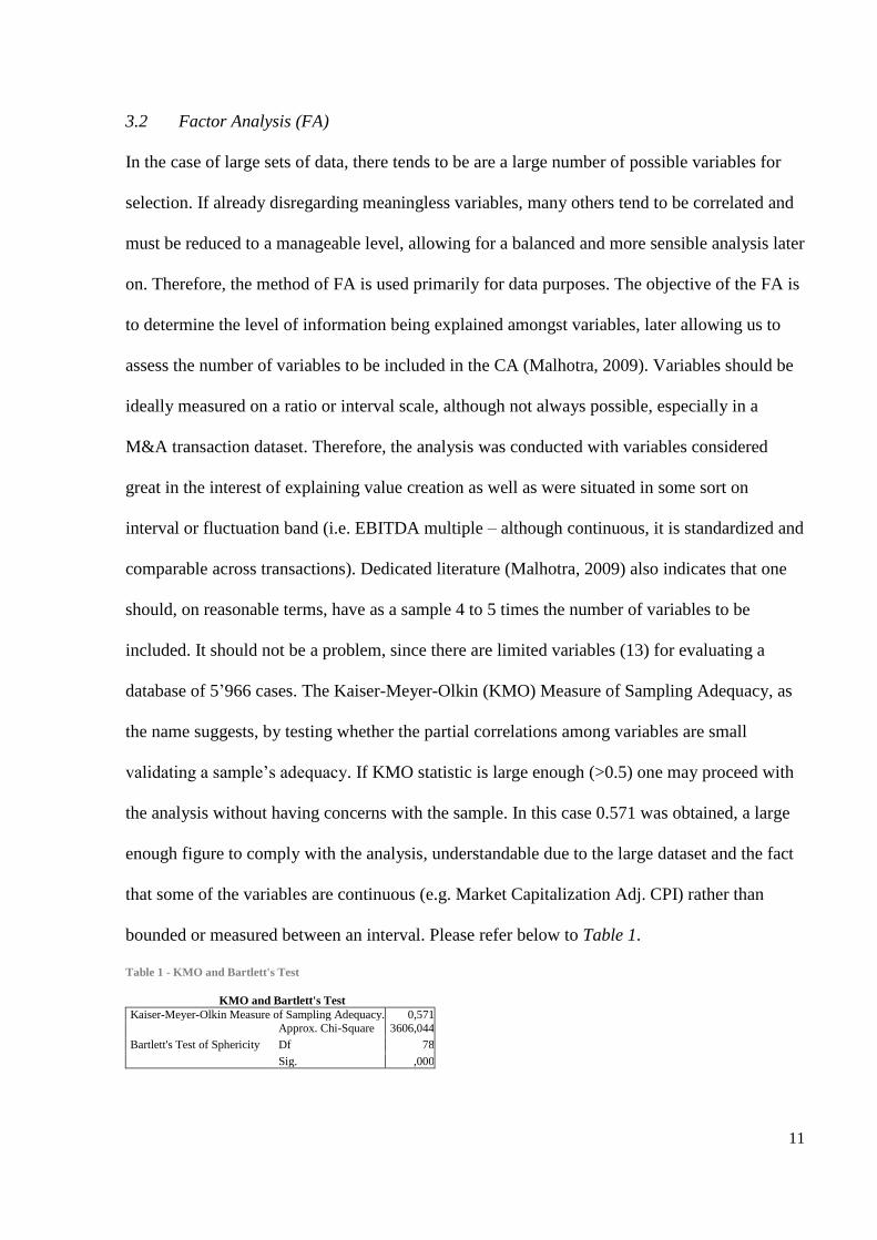
bounded or measured between an interval. Please refer below to Table 1.

Table 1 - KMO and Bartlett's Test

KMO and Bartlett's Test

Kaiser-Meyer-Olkin Measure of Sampling Adequacy. 0,571

Bartlett's Test of Sphericity

Approx. Chi-Square 3606,044

Df 78

Sig. ,000

12

The next step of the FA is to obtain a correlation matrix and identify variables which may

provide the same level of information and are not suited to be added together to the CA –

please refer to Table 2 in the Appendix. Before obtaining the from correlation matrix an

obvious fact that all valuation multiples were strongly correlated, did provide the same

information level and in some industries (e.g. Financials) some valuation multiples, namely

EBITDA multiple, was not available. For that reason the valuation metric of choice is the Total

Asset Multiple, the most complete in the database. Furthermore, the correlation matrix was

very useful to understand that, the variables (Intra)Extrasector and (In)Cross border provided a

limited degree of information and a better variable good be reached, the Ansoff Matrix 1-4.

Now one could use the two variables to achieve both the level of product and market growth

strategy from each transaction (Ansoff, 1957). The Ansoff Matrix presented and assigned

points according to the degree of growth and risk for every one of four growth strategies:

Market Penetration (1 point; same market, same product line); Market Development (2 points;

new/different market, same product line); Product Development (3 points; same market,

new/different product line); and finally, Diversification (4 points; different market, different

product line). Despite the insight of the new variable, all the three variables were included in

the FA for review purposes.

Provided the above literature review and dataset, the pre-selected variables for the CA were the

following: Ansoff Matrix Growth Strategies, PE/VC Involvement, Nature of the Bid, Total

Assets Multiple, Market Capitalization of Acquirer Adjusted to CPI, Target Announced

Amount Adjusted to CPI, Relative Size (% Market Cap.), Cash Terms, Deal Experience,

Tender Offer, Competing Factor, (In)Cross border, (Intra)Extrasector – please refer to Table 2.

Proceeding with the selection of variables for FA, the Bartlett’s test for sphericity is conducted,

which tests the hypothesis that the correlation matrix is an identity matrix. If its null hypothesis

was verified it would indicate that the variables are unrelated and therefore unsuitable for

13

structure detection. Inability to form a structure would mean that we would not be able to build

a factor out of any two or more variables, therefore eliminating the possibility of FA. Bartlett’s

test performed reached a significance of .000 (Table 1) which means that for any level of

significance we have enough evidence to reject the null hypothesis of being in presence of an

identity matrix. When performing and interpreting the FA, the number of factors can be

determined (1) à priori or (2) by interpretation, usually a result of the eigenvalues, total

variance explained per factor and interpretation of the scree plot (Figure 2) (Malhotra, 2009). À

priori would mean the factors are already known beforehand and that, factoring would only

help understand which of the presented variables fit which factor and how well - i.e. a

consumer’s rationale to buy toothpaste, the health benefit factor and aesthetic factor - which is

not the case. In this situation, the percentage of explained variance in each factor helps one to

understand the contribution of each variable to the total variance explained and get to the ideal

number of components to be later on included in the CA. The analysis turned out to be very

balanced by both interpreting the scree plot (Figure 2) and table of total variance explained

(Table 4). Total variance explained, indicated by initial eigenvalues, accumulated and

individual variances were different between all variables and percentage of variance ranging

between 4.116-14.165% (Table 4). Additionally, from the scree plot there is an indication that

the number of components should be between 5 and 6, close to the recommended 1.0 threshold

level by literature (Malhotra, 2009). From the sixth component onwards the eigenvalue levels

starts to marginally decrease for each component added to the scree plot. This part although

based in the fundamental research (Malhotra, 2009) is as much an art as it is a science. For this

case, there is the tendency to be close to the maximum bound of components possible for the

CA, as it provides for richer analysis later on. However, including too many components has

the risk of not being research supported and being difficult to define causality later on in the

CA. Therefore, the line not to be crossed was determined at the marginal decrease of

14

eigenvalues, which determines 7 to be the maximum components to be included, fairly close to

the 1.0 threshold suggested in the literature, with 0.974 eigenvalue and 7.489% of individual

variance for the seventh and final component (Figure 2). Since factors might take the

economical meaning out of variable one could indeed select surrogate variables - variables that

best substitute each factor - those with the higher loadings that help explain the most

(percentage of variance) and those that à priori do make sense to be included. (Malhotra, 2009).

After having identified from the Literature Review that these variables are adequate in

explaining CAR, the use of surrogate variables provided for better economic interpretation

instead of the factors and, knowing that each of these variables together leaves very little room

for unexplained variation, the next step was to perform a CA with the present variables (Table

2). We selected a Principal Component Analysis (PCA) extraction method and Varimax with

Kaiser Normalization for the rotation method for the FA as suggested by the main literature

(Malhotra, 2009). PCA is a non-parametric method for extracting relevant information from

“confusing” data sets (Shlens, 2009). Varimax seeks that “for each factor, high loadings

(correlations) will result for a few variables; the rest will be near zero" (Kaiser, 1958).

Out of the 13 rotated variables, the 7 components selected for CA and segmentation from the

FA are: Ansoff Matrix Growth Strategies, PE/VC Involvement, Nature of the Bid, Total Assets

Multiple, Market Capitalization of Acquirer Adjusted to CPI, Relative Size (% Market Cap.)

and Cash Terms.

3.3 Cluster Analysis (CA)

Cluster analysis is a “class of techniques used to classify objects or cases in relatively

homogenous groups called clusters” (Malhotra, 2009). Also designated as classification

analysis or numerical taxonomy, it allows the researcher to classify or segment data. It is of

particular importance to this research to let data “speak for itself” making possible, with the

right methodology, to segment Global M&A transactions and help understand which segments

15

are formed. Additionally it fits perfectly to the problem in hands, as a CA with the right

methodology is able to handle both continuous and categorical variables/attributes while. In

this case it suits perfectly, since the balance and judgment of the research can only help one

reach so far, especially the ultimate purpose is to determine how many clusters it will

“naturally” form. However, if we fixed the number of clusters, without any paramount reason

we might be damaging the balance between the ideal number of clusters and the model’s

balance.

The first step to conducting CA is to select the variables. In our case, having done the CA and

literature review the variables are already pre-selected. Secondly, one should define the method

of clustering. A distance measure will help determine how similar or dissimilar the objects

being clustered, as explained later on. Thirdly, one should determine the appropriate number of

clusters. After the validity of the clustering process is assessed the economic interpretation

from the CA is drawn. When selecting the variables these should be “variables that best explain

the distribution into the groups we have found” (Berrendero, Justel, & Svarc, 2011). Since both

the Literature Review and the FA validate the variables selected, “non-informative” variables

that are innocuous, redundant or strongly correlated information are excluded. It has two steps:

1) pre-cluster the cases (or records) into as many pairs according to their similarity; 2) group

these sub-clusters into the desired number of clusters or as a result of an optimization process

that a process that automatically decides the number of clusters. In the present case the method

chosen was a two-step CA. The method is a scalable algorithm designed to handle very large

sets of data and be setup to either segment into a prefixed number of clusters or to instead allow

it, through a clustering criterion, to automatically determine the number of cluster (IBM, 2012).

Three important metrics define the success and quality of the clustering process: (1) how many

and which variables are selected and of these, which are categorical, continuous and of the

continuous, which are assumed to be and which need to be standardized; (2) the distance

16

measure applied to define the clusters, the actual algorithm of the two-step method; (3) and

finally, the clustering criterion. The first step has been largely facilitated by the CA, having

only to identify which of the variables are categorical, standardized continuous and to be

standardized continuous variables. In the second step one assigns the log-likelihood measure.

The log-likelihood was selected as it is a distance measure that can handle both continuous and

categorical variables. It is a probability based distance. In calculating log-likelihood, normal

distributions for continuous variables and multinomial distributions for categorical variables are

assumed. One main assumption is that the variables are independent of each other, and so are

the cases, reason for the correlation analysis undertaken with the FA. IBM SPSS User Guide

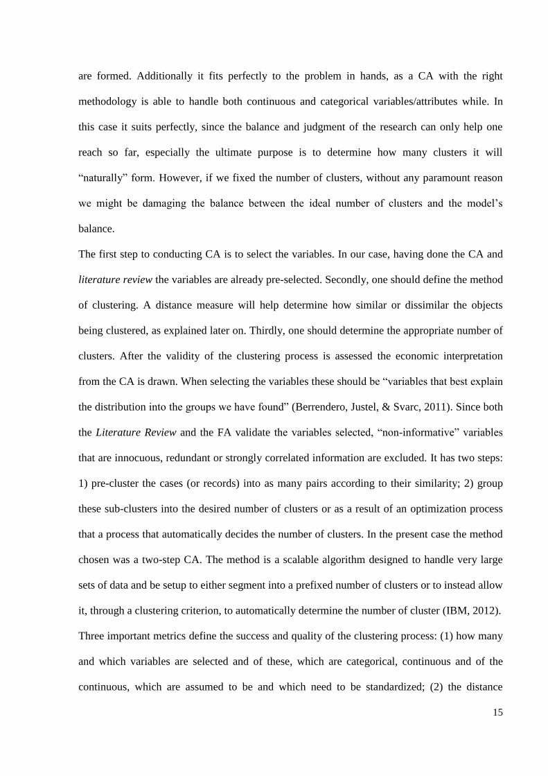
provides the steps for the actual the distance between a given cluster is as being defined by:

Equation 2 - Distance between to clusters related to the decrease in log-likelihood as they are combined into one cluster

where, and .

N Number of data records in total.

Nk Number of data records in cluster k.

The estimated mean of the kth continuous variable across the entire dataset.

The estimated variance of the kth continuous variable across the entire dataset.

The estimated variance of the kth continuous variable across the entire dataset.

Nvkl Number of data records in cluster j whose kth categorical variable takes the lth category.

Nkl Number of data records in the kth categorical variable that take the lth category.

d(j, s) Distance between clusters j and s.

(j,s) Index that represents the cluster formed by combining clusters j and s.

If is ignored in Equation 2, the distance between clusters j and s would be exactly the

decrease in log-likelihood when the two clusters are combined. The term is added to solve

the problem caused by , which would result in the natural logarithm being undefined

(this would occur, for example, when a cluster only has one case) (Ming-Yi, Jheng, & Lien-Fu,

2010). IBM SPSS provides the user with the option to consider the dataset to have outliers. In

the present case, due to the large dataset a higher interest in having more sound “averages”

rather than understanding ranges, minimum or maximum bounds, the outlier-handling helps to

17

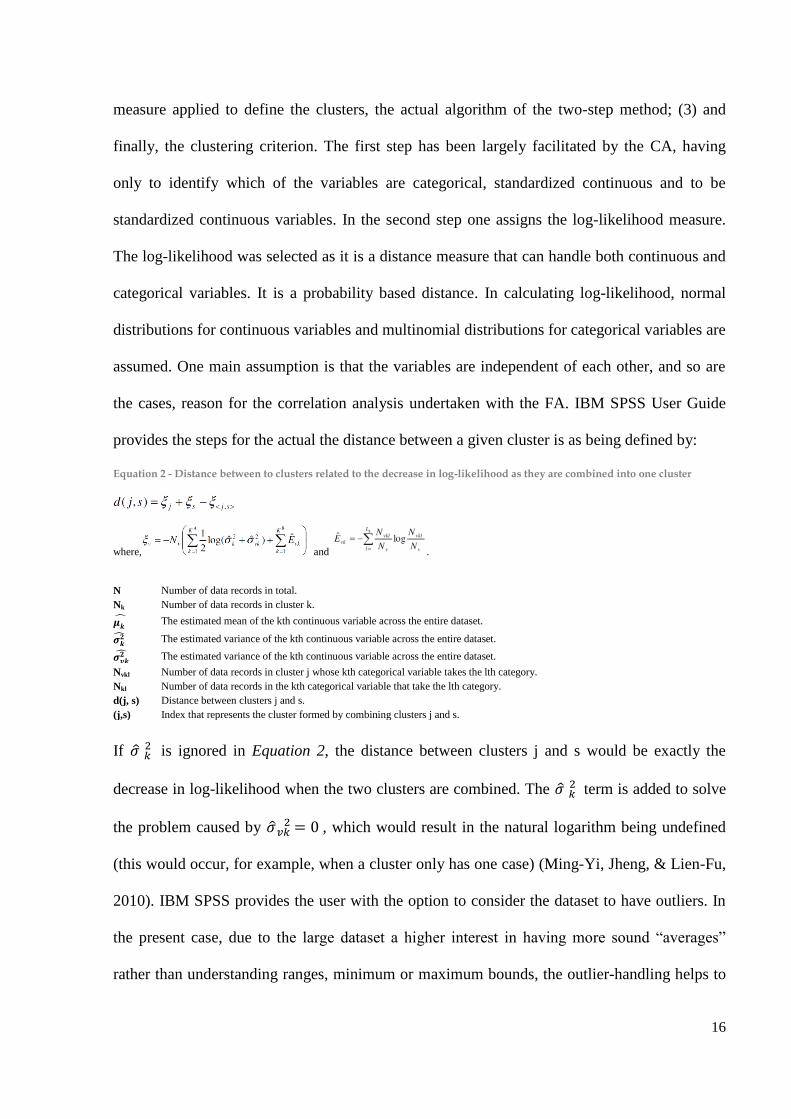
offset exaggerations or erroneous inputs from Bloomberg. The log-likelihood distance assumes

outliers or noises to follow a uniform distribution. The method goes about calculating log-

likelihood to assigning a record to a noise-cluster and that resulting from assigning it to the

closest non-noise cluster. Subsequently, the record is assigned to the cluster with the cluster

which leads to the largest log-likelihood.

Equation 3 - Log-likelihood distance

, where ∏ ∏ .

Otherwise, it is designated as an outlier defined by IBM SPSS under the cluster (-1).

The clustering criterion assigned was the Bayesian Information Criterion (BIC) which has the

advantage to determine the number of components in a model and deciding between which two

or more groups most closely matches the data for a given model (Fraley & Raftery, 1998). IBM

SPSS allowed for all major methods of clustering. Fraley and Raftery (1998) found that after

clinically assigning each case to the known à priori best cluster for each, they measured error

rates for Model-based Classification (BIC), Single Link (Nearest Neighbor) and K-Means, and

found out, with corresponding 12%, 47% and 36%, being that a Model-based produced less

error in assignment, in addition to being able to treat categorical and continuous variables.

Missing values are treated on a Listwise basis by SPP. However, the dataset presented no

missing values.

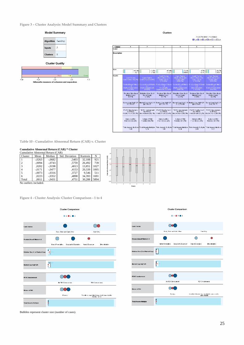
Overall clustering success can be measured by the silhouette coefficient, which is a measure of

both cohesion and separation (Norušis, 2011). In our model the average silhouette is of 0.7,

with a very good result being above the 0.5 mark, above 0.2 considered moderate-to-fair and

below 0.2 a bad result, according to IBM IPSS (Model Summary – Figure 3)

18

4. Conclusion

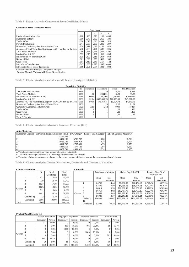
Having performed a two-step cluster analysis, the process yielded 6 segments from 7 variables.

The 7 variables were selected out of 13 from the CA. The input with higher predictor

importance was the Ansoff Matrix Growth Strategy and the Cash Terms variables (Figure 4).

Out of all clusters there is a strong grouping affect in regards toward growth strategy. Market

Penetration is the dominant strategy in Global M&A (Figure 4). Valuations are more favorable

for a market penetration growth strategy (Cluster 1, 6) and do not depend on the acquirer’s size,

the Relative Size of the target (percentage of the acquirer’s market capitalization), the Nature of

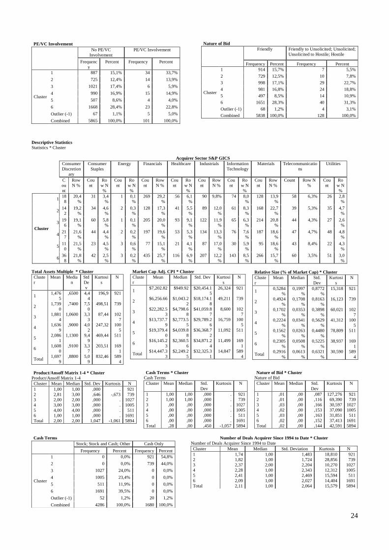
the Bid or the Terms of Deal (cash/stock/cash and stock/other) (Table 9). PE/VC involvement

is inversely related to the dimension of growth strategy pursued amongst the clusters, although

worth mentioning PE/VC involvement is generally low across all six clusters, bounded between

1-4%. The extremes are Cluster 5 (Diversification) with only 0.8% of its transactions with

PE/VC involvement compared to Cluster 1 (Market Penetration) that 3.7%, more than four

times Cluster 5 (Table 7). The same happens with the nature of transactions. Market

Penetration (Cluster 1, 6) has relatively more friendly deals (99.2%) when compared to

Geographic Expansion (97.2%) and Market Expansion (98.6%) and even more when compared

against Diversification strategies (97.3%) (Table 9). The clusters seem to suggest that as

companies initiate M&A transactions with geographic and new market growth strategies, they

tend to face relatively more non-friendly bidding processes before completing the transactions

(friendly-to-unsolicited, unsolicited, unsolicited-to-hostile and hostile). The Materials sector,

which comprises Chemicals, Construction Materials, Metals & Mining and Paper & Forest

Products, although a generally dominant sector across all clusters, in the case of Geographic or

Market Expansion (Cluster 2, 3 and 5) rank either first and second in absolute and relative

terms across all 10 industry groups. Clusters with cash financing strategies in 100% of the cases

are associated with relatively smaller acquirers/dominant counterparties. These small acquirers

19

(Cluster 1, 2) have an average of $7.20 and $6.26 billion (market capitalization at the

announcement date) compared to the other clusters ranging from $13.74 - $19.38 billion

(Cluster 3, 4, 5, 6); Clusters formed by small size companies seem to point to fully-financed

cash transactions, being the inverse equally true, larger firms tend to have equity financing in

completed bids. With the effect of outliers exempt in the CA, Clusters 3, 5, 6 present higher

median Cumulative Abnormal Returns (CAR) with -1.98%, -3.16% and -3.52%, respectively

(Table 10). From a growth strategy point-of-view it does not seem possible to establish a linear

relation between the Ansoff Matrix point system and corresponding levels of return (CAR).

Across all clusters, CAR is on average +0.11%, a small figure to argue for value M&A creation

excluding outliers and a lower +0.9% with the effect of outliers. Although, overall skewness is

positive (mean>median) which leads us to conclude that there are few very positive

transactions that outweigh a larger number of less negative transactions, 50% of the cases

(median) have CARs of no more than -4.5% over the period of one year for acquiring

shareholders (Table 10)

More importantly and touching on the methodology and innovative side of the paper, even

though other variables could have been different as could the overall study been done

differently, the main proposed objectives were achieved. The implementation of having

surrogate variables and an automatic clustering criterion ended up being the best

methodological framework for the thesis, as both increase economical interpretation of the

rotated set of components and the clusters are “natural” groupings, not conducted or forced in

anyway.

20

References

[1] Ansoff, I. H. (Sep-Oct de 1957). Strategies for Diversification. Harvard Business Review, pp.

113-124.

[2] Asquith, P. (1983). Merger bids, uncertainty, and stockholder returns. Journal of Financial

Economics, 51-83.

[3] Berrendero, J. R., Justel, A., & Svarc, M. (1 de September de 2011). Principal components for

multivariate functional data. Computational Statistics & Data Analysis, pp. 2619–2634.

[4] Bruner, R. J. (2002). Does M&A pay? A survey of evidence for the decision-maker. Journal of

Applied Finance, 2-15.

[5] Bureau of Labor Statistics. (September de 2010). Frequently Asked Questions (FAQ) - "What is

the CPI?". Obtido de Consumer Price Index - U.S. Bureau of Labor Statistics:

http://www.bls.gov/cpi/cpifaq.htm

[6] Chen, C., & Findlay, C. (2003). A Review of Cross-border Mergers and Acquisitions in APEC.

[7] Cyriac, J., Koller, T., & Thomsen, J. (February de 2012). McKinsey on Finance, pp. 8-15.

[8] Datta, D. K., Pinches, G. E., & Narayanan, V. K. (1992). Factors Influencig Wealth Creation

from Mergers and Acquisitions: A Meta-Analysis. Strategic Management Journal, 13, pp. 67-84.

[9] Fraley, C., & Raftery, A. E. (1998). How Many Clusters? Which Clustering Method? Answers

via Model-Based Cluster Analysis. The Computer Journal, Vol.41, No.8, pp. 578-588.

[10] Hoang, T. V., & Lapumnuaypon, K. (2007). Critical Success Factors in Merger & Acquisition

Projects: A Study from the Perspective of Advisory Firms.

[11] IBM. (2012). IBM SPSS Statistics 21 Documentation. IBM Corporation:

ftp://public.dhe.ibm.com/software/analytics/spss/documentation/statistics/21.0/en/client/Manuals/IB

M_SPSS_Statistics_Core_System_Users_Guide.pdf

[12] Ikenberry, D., Lakoniskok, J., & Vermaelen, T. (1995). Market underreaction to open market

share repurchases. Journal of Financial Economics, 181-208.

[13] Kaiser, H. F. (1958). The varimax criterion for analytic rotation in factor analysis.

Psycometrika, Vol. 23, 187-200.

[14] Malhotra, N. K. (2009). Marketing Research: An Applied Orientation. Prentice Hall; 6th edition

.

[15] Megginson, W. L., Morgan, A., & Nail, L. (2004). The determinantes of positve long-term

performance in strategic mergers: corporate focus and cash. Journal of Banking & Finance, 523-552.

[16] Ming-Yi, S., Jheng, J.-W., & Lien-Fu, L. (2010). A Two-Step Method for Clustering Mixed

Categroical.

[17] Norušis, M. (2011). Chapter 17 - Cluster Analysis. In IBM SPSS Statistics Guides (pp. 375-

404). Addison Wesley.

[18] Shlens, J. (2009). A Tutorial on Principal Component Analysis. NY, USA: Central for Neural

Science, New York University.

[19] Tiemann, D. D., & Kelly, J. (2010). The Determinants of M&A Sucess: What Factors

Contribute to Deal Success? KPMG Advisory, pp. 5-13.

21

Appendices

Figure 1 – Sample evolution: number of filters, description and cases reached after each filter.

Filters

(0) Unfiltered, from 01/Jan/1900 to 31/Dec/2012: 367’438 results; (1) Deal Status = {Completed}: 347’273 results;

(2) Deal Size = Min=$ 0.0001mn; Max= ∞ -. Requires that each deal has its size

disclosed: 198’303;

(3) Payment Type = {Cash, Stock, Cash AND Stock, Cash OR Stock, Cash

AND Debt, Cash AND Stock AND Debt, Stock AND Debt, Debt} OR

{NOT Undisclosed} – deal terms are known: 174’814 results;

(4) Announced Premium = {Min = -100%; Max = ∞ } - premium is known, which in turn

means the acquired firm is publicly listed: 29’126 results;

(5) Acquirer = {Public}, acquirer is publicly listed, essential to later

measure abnormal returns: 14’111 results;

(6) Elimination of duplicated deals: 14’059 results; Errors of Bloomberg’s database. (7) Elimination of deals with Multiple Acquirers, not being able to measure

Acquirer 1 year Total Return : 12’703 results;

(8) Modification of the related index of 64 deals for the S&P 500 Index. Each deal had

associated its local country index (i.e. Portugal – PSI20 Index) allowing for a better and

more comparable measure of Cumulative Abnormal Return (CAR). Exceptionally, and in

the case of these 64 deals, S&P 500 Index was the used index of replacement since it is

the most representative within the sample – most acquirers are US based: 12’703 results;

(9) Omission of missing cases with missing values: 5’966

Table 2 – Factor Analysis: Input Variables

Variable Input

Number of Bidders (Competition Factor) 1 = At least one competing bid; 0 = No competing bid

Tender Offer 1 = Yes; 0 = No, tender offer

PE/VC Involvement 1 = PE and VC, VC or PE involved; 0 = No PE or VC involved

Number of Deals (Since 1994-to-date) Count of the number of deals per bidder

Announced Total Value Adjusted to 2011 dollars Announced Value adjusted to present value (2011) by the rate of inflation (CPI)

Market Capitalization of Acquirer Market Capitalization of the Acquirer at the announcement of the completion adjusted by the same CPI rate

Relative Size (% Market Cap) Announced Total Value Adj. 2011 / Market Capitalization of Acquirer

Nature of Bid 0 = Friendly; 1 = Friendly to Unsolicited; Unsolicited; Unsolicited to Hostile; Hostile

Cash Terms 0 = Cash (only); 1 = Stock; Stock and Cash; Other

In border/Cross border 0 = In border; 1 = Cross border

Intrasector/Extrasector 0 = Intrasector; 1 = Extrasector

Ansoff Growth Strategies 1-4 1 = Market Penetration; 2 = Geographic Expansion; 3 = Market Expansion; 4 = Diversification

Table 3 – Factor Analysis: Correlation Matrix and Communalities

Product/

Ansoff

Matrix 1-

4

Number

of

Bidders

Tender

Offer

PE/VC

Involvement

Number of

Deals

Acquirer

Since 1994

to Date

Announced

Total Valued

(mil) Adj.

2011 CPI

Total

Assets

Multiple

Market

Cap

Adj.

CPI

Relative

Size (% of

Market

Cap)

Nature

of Bid

Cash

Terms

In /

Cross-

boarder

Intra/Cross-

sector

Transaction

Correlation

Product/Ansoff

Matrix 1-4

1,000 -,012 ,047 -,029 ,071 -,019 ,029 ,041 -,036 ,016 -,119 ,204 ,223

Number of Bidders -,012 1,000 ,074 -,011 ,019 -,003 ,001 ,008 -,012 ,058 -,034 ,043 -,010

Tender Offer ,047 ,074 1,000 -,068 ,050 -,018 -,009 ,019 -,018 ,043 -,124 ,062 ,008

PE/VC

Involvement

-,029 -,011 -,068 1,000 -,061 ,076 -,004 -,024 ,042 -,019 ,068 -,051 -,017

Number of Deals

Acquirer Since

1994 to Date

,071 ,019 ,050 -,061 1,000 ,034 ,005 ,412 -,096 ,009 -,104 ,098 ,108

Announced Total

Valued (mil)

Adjusted to 2011

dollars by the Con

-,019 -,003 -,018 ,076 ,034 1,000 ,003 ,198 ,084 ,093 ,062 ,013 -,062

Total Assets

Multiple

,029 ,001 -,009 -,004 ,005 ,003 1,000 ,006 -,004 -,001 -,011 ,032 ,012

Market Cap Adj.

CPI

,041 ,008 ,019 -,024 ,412 ,198 ,006 1,000 -,084 ,014 -,126 ,174 ,087

Relative Size (%

Market Cap)

-,036 -,012 -,018 ,042 -,096 ,084 -,004 -,084 1,000 ,024 ,139 -,076 -,065

Nature of Bid ,016 ,058 ,043 -,019 ,009 ,093 -,001 ,014 ,024 1,000 -,049 ,053 -,008

Cash Terms -,119 -,034 -,124 ,068 -,104 ,062 -,011 -,126 ,139 -,049 1,000 -,291 -,123

In / Cross-boarder ,204 ,043 ,062 -,051 ,098 ,013 ,032 ,174 -,076 ,053 -,291 1,000 -,021

Intra/Cross-sector

Transaction

,223 -,010 ,008 -,017 ,108 -,062 ,012 ,087 -,065 -,008 -,123 -,021 1,000

a. Determinant = .546

Communalities

Initial Extraction

Product/Ansoff Matrix 1-4 1,000 ,616

Number of Bidders 1,000 ,321

22

Tender Offer 1,000 ,393

PE/VC Involvement 1,000 ,269

Number of Deals Acquirer Since 1994 to Date 1,000 ,632

Announced Total Valued (mil) Adjusted to 2011 dollars by the Con 1,000 ,583

Total Assets Multiple 1,000 ,266

Market Cap Adj. CPI 1,000 ,708

Relative Size (% of Market Cap) 1,000 ,384

Nature of Bid 1,000 ,429

Cash Terms 1,000 ,494

In-border / Cross-boarder 1,000 ,636

Intra-sector/Cross-sector Transaction 1,000 ,714

Extraction Method: Principal Component Analysis.

Table 4 - Factor Analysis: Total Variance Explained Figure 2 – Factor Analysis: Scree Plot

Total Variance Explained

Compo

nent

Initial Eigenvalues Extraction Sums of Squared

Loadings

Rotation Sums of Squared

Loadings

Total % of

Varianc

e

Cumulat

ive %

Total % of

Varianc

e

Cumulat

ive %

Total % of

Varianc

e

Cumulat

ive %

1 1,842 14,165 14,165 1,842 14,165 14,165 1,506 11,588 11,588

2 1,314 10,110 24,275 1,314 10,110 24,275 1,329 10,222 21,810

3 1,175 9,039 33,315 1,175 9,039 33,315 1,237 9,516 31,326

4 1,094 8,415 41,730 1,094 8,415 41,730 1,204 9,261 40,587

5 1,020 7,844 49,574 1,020 7,844 49,574 1,168 8,988 49,574

6 ,990 7,618 57,192

7 ,974 7,489 64,681

8 ,935 7,194 71,876

9 ,899 6,918 78,793

10 ,824 6,342 85,135

11 ,783 6,022 91,157

12 ,614 4,727 95,884

13 ,535 4,116 100,000

Extraction Method: Principal Component Analysis.

Table 5 - Factor Analysis: Component Matrix, Rotated Component Matrix and Transformation Matrix

Component Matrix

Component

1 2 3 4 5

Product/Ansoff Matrix 1-4 ,418 -,305 -,155 ,554 ,133

Number of Bidders ,095 -,034 ,457 -,142 ,285

Tender Offer ,235 -,186 ,423 -,166 ,311

PE/VC Involvement -,194 ,234 -,115 ,379 -,142

Number of Deals Acquirer Since 1994 to Date ,578 ,383 -,236 -,273 ,146

Announced Total Valued (mil) Adjusted to 2011 dollars by the Con ,052 ,674 ,181 ,305 ,001

Total Assets Multiple ,056 -,037 -,022 ,237 -,453

Market Cap Adj. CPI ,598 ,557 -,146 -,137 -,008

Relative Size (% of Market Cap) -,322 ,209 ,177 ,395 ,220

Nature of Bid ,109 ,130 ,515 ,279 ,240

Cash Terms -,572 ,297 -,191 -,001 ,203

In-border / Cross-boarder ,554 -,113 ,300 ,180 -,440

Intra-sector/Cross-sector Transaction ,343 -,236 -,466 ,296 ,486

Extraction Method: Principal Component Analysis.

a. 5 components extracted.

Rotated Component Matrix

Component

1 2 3 4 5

Product/Ansoff Matrix 1-4 -,039 ,322 ,709 ,088 -,021

Number of Bidders -,006 -,003 -,077 ,064 ,557

Tender Offer ,004 ,076 ,049 -,075 ,616

PE/VC Involvement -,071 -,005 ,021 ,374 -,352

Number of Deals Acquirer Since 1994 to Date ,776 -,008 ,106 -,119 ,063

Announced Total Valued (mil) Adjusted to 2011 dollars by the Con ,335 ,029 -,139 ,669 -,055

Total Assets Multiple -,094 ,393 -,047 ,064 -,311

Market Cap Adj. CPI ,826 ,135 ,009 ,087 -,020

Relative Size (% of Market Cap) -,215 -,201 ,044 ,542 ,029

Nature of Bid -,034 ,136 ,050 ,464 ,439

Cash Terms -,113 -,593 -,159 ,234 -,222

In-border / Cross-boarder ,119 ,784 ,020 ,009 ,084

Intra-sector/Cross-sector Transaction ,142 -,147 ,814 -,099 -,011

Extraction Method: Principal Component Analysis.

Rotation Method: Varimax with Kaiser Normalization.a

a. Rotation converged in 6 iterations.

Component Transformation Matrix

Component 1 2 3 4 5

1 ,650 ,573 ,394 -,170 ,255

2 ,648 -,221 -,373 ,601 -,176

3 -,249 ,350 -,413 ,353 ,722

4 -,296 ,280 ,545 ,685 -,261

5 ,091 -,649 ,488 ,131 ,561

Extraction Method: Principal Component Analysis.

Rotation Method: Varimax with Kaiser Normalization.

23

Table 6 - Factor Analysis: Component Score Coefficient Matrix

Component Score Coefficient Matrix

Component

1 2 3 4 5

Product/Ansoff Matrix 1-4 -,108 ,193 ,570 ,139 -,055

Number of Bidders -,016 -,047 -,065 ,060 ,489

Tender Offer -,026 -,010 ,020 -,044 ,528

PE/VC Involvement -,044 ,053 ,053 ,309 -,297

Number of Deals Acquirer Since 1994 to Date ,529 -,118 ,032 -,101 ,029

Announced Total Valued (mil) Adjusted to 2011 dollars by the Con ,230 ,034 -,091 ,548 -,045

Total Assets Multiple -,098 ,366 -,068 ,062 -,307

Market Cap Adj. CPI ,553 ,019 -,051 ,069 -,053

Relative Size (% of Market Cap) -,135 -,122 ,111 ,454 ,063

Nature of Bid -,061 ,083 ,059 ,409 ,380

Cash Terms ,004 -,415 -,043 ,157 -,124

In-border / Cross-boarder -,012 ,607 -,075 ,043 -,009

Intra-sector/Cross-sector Transaction ,066 -,226 ,684 -,032 -,009

Extraction Method: Principal Component Analysis.

Rotation Method: Varimax with Kaiser Normalization.

Table 7 - Cluster Analysis: Variables and Cluster Descriptive Statistics

Descriptive Statistics

N Minimum Maximum Mean Std. Deviation

Two-step Cluster Number 5966 -1 6 3,71 1,869

Total Assets Multiple 5966 ,00 2984,91 2,29 39,28

Relative Size (% of Market Cap) 5966 0,00% 66,54% 0,3391% 1,29475%

Market Cap Adj. CPI 5966 $2.24 $536,405.70 $16,973.53 $43,627.58

Announced Total Valued (mil) Adjusted to 2011 dollars by the Con 5966 $0.00 $96,450.25 $1,024.73 $4,349.96

Number of Deals Acquirer Since 1994 to Date 5966 1 23 2,15 2,161

Cumulative Abnormal Return (CAR) 5966 -2,10 6,42 -,0009 ,47417

Tender Offer 5966 0 1 ,28 ,450

Cash Terms 5966 0 1 ,28 ,450

Nature of Bid 5966 0 1 ,02 ,145

Valid N (listwise) 5966 - - - -

Table 8 - Cluster Analysis: Schwarz's Bayesian Criterion (BIC)

Auto-Clustering

Number of Clusters Schwarz's Bayesian Criterion (BIC) BIC Changea Ratio of BIC Changesb Ratio of Distance Measuresc

1 21114,837

2 15414,105 -5700,732 1,000 1,210

3 10719,186 -4694,919 ,824 1,707

4 8011,732 -2707,453 ,475 1,579

5 6334,611 -1677,121 ,294 1,160

6 4902,791 -1431,820 ,251 1,965

a. The changes are from the previous number of clusters in the table.

b. The ratios of changes are relative to the change for the two cluster solution.

c. The ratios of distance measures are based on the current number of clusters against the previous number of clusters.

Table 9 - Cluster Analysis: Cluster Distribution, Centroids and Clusters v. Variables

Cluster Distribution

N % of

Combined

% of

Total

Cluster

1 921 15,4% 15,4%

2 739 12,4% 12,4%

3 1027 17,2% 17,2%

4 1005 16,8% 16,8%

5 511 8,6% 8,6%

6 1691 28,3% 28,3%

Outlier (-1) 72 1,2% 1,2%

Combined 5966 100,0% 100,0%

Total 5966 100,0%

Centroids

Total Assets Multiple Market Cap Adj. CPI Relative Size (% of

Market Cap)

Mean Std.

Deviation

Mean Std.

Deviation

Mean Std.

Deviation

Cluster

1 1,4765 4,44 $7,202.82 $20,454.15 0,5284% 0,8772%

2 1,7390 7,50 $6,256.66 $18,174.18 0,4924% 0,8163%

3 1,8814 3,33 $22,282.53 $41,059.87 0,1702% 0,3898%

4 1,6369 4,02 $13,737.79 $29,789.26 0,2224% 0,5629%

5 2,0861 9,49 $19,379.40 $36,368.72 0,1562% 0,4480%

6 1,6080 3,37 $16,145.23 $34,871.24 0,2305% 0,5225%

Outlier (-

1)

50,6589 353,67 $223,771.11 $171,123.75 4,2314% 9,5981%

Combined 2,2888 39,28 $16,973.53 $43,627.58 0,3391% 1,2947%

Product/Ansoff Matrix 1-4

Market Penetration Geographic Expansion Market Expansion Diversification

Frequency Percent Frequency Percent Frequency Percent Frequency Percent

Cluster

1 921 34,9% 0 0,0% 0 0,0% 0 0,0%

2 0 0,0% 235 18,5% 406 28,4% 98 15,7%

3 0 0,0% 1027 80,7% 0 0,0% 0 0,0%

4 0 0,0% 0 0,0% 1005 70,3% 0 0,0%

5 0 0,0% 0 0,0% 0 0,0% 511 81,8%

6 1691 64,1% 0 0,0% 0 0,0% 0 0,0%

Outlier (-1) 26 1,0% 11 0,9% 19 1,3% 16 2,6%

Combined 2638 100,0% 1273 100,0% 1430 100,0% 625 100,0%

24

PE/VC Involvement

No PE/VC

Involvement

PE/VC Involvement

Frequenc

y

Percent Frequency Percent

Cluster

1 887 15,1% 34 33,7%

2 725 12,4% 14 13,9%

3 1021 17,4% 6 5,9%

4 990 16,9% 15 14,9%

5 507 8,6% 4 4,0%

6 1668 28,4% 23 22,8%

Outlier (-1) 67 1,1% 5 5,0%

Combined 5865 100,0% 101 100,0%

Descriptive Statistics

Statistics * Cluster

Acquirer Sector S&P GICS

Consumer

Discretion

ary

Consumer

Staples

Energy Financials Healthcare Industrials Information

Technology

Materials Telecommunicatio

ns

Utilities

C

ou

nt

Row

N %

Cou

nt

Ro

w N

%

Cou

nt

Ro

w N

%

Cou

nt

Row

N %

Cou

nt

Ro

w N

%

Cou

nt

Row

N %

Cou

nt

Ro

w N

%

Cou

nt

Row

N %

Count Row N

%

Cou

nt

Ro

w N

%

Cluster

1 18

8

20,4

%

31 3,4

%

1 0,1

%

269 29,2

%

56 6,1

%

90 9,8% 74 8,0

%

128 13,9

%

58 6,3% 26 2,8

%

2 14

2

19,2

%

34 4,6

%

2 0,3

%

128 17,3

%

41 5,5

%

89 12,0

%

61 8,3

%

168 22,7

%

39 5,3% 35 4,7

%

3 19

6

19,1

%

60 5,8

%

1 0,1

%

205 20,0

%

93 9,1

%

122 11,9

%

65 6,3

%

214 20,8

%

44 4,3% 27 2,6

%

4 21

7

21,6

%

44 4,4

%

2 0,2

%

197 19,6

%

53 5,3

%

134 13,3

%

76 7,6

%

187 18,6

%

47 4,7% 48 4,8

%

5 11

0

21,5

%

23 4,5

%

3 0,6

%

77 15,1

%

21 4,1

%

87 17,0

%

30 5,9

%

95 18,6

%

43 8,4% 22 4,3

%

6 36

8

21,8

%

42 2,5

%

3 0,2

%

435 25,7

%

116 6,9

%

207 12,2

%

143 8,5

%

266 15,7

%

60 3,5% 51 3,0

%

Total Assets Multiple * Cluster

Cluste

r

Mean Media

n

Std

De

v

Kurtosi

s

N

1 1,476

5

,6500 4,4

4

196,9 921

2 1,739

0

,7400 7,5

0

498,51 739

3 1,881

4

1,0600 3,3

3

87,44 102

7

4 1,636

9

,9000 4,0

2

247,32 100

5

5 2,086

1

1,1300 9,4

9

469,44 511

6 1,608

0

,9100 3,3

7

203,51 169

1

Total 1,697

9

,8800 5,0

9

832,46 589

4

Market Cap Adj. CPI * Cluster

Cluste

r

Mean Median Std. Dev Kurtosi

s

N

1 $7,202.82 $949.92 $20,454.1

5

26,324 921

2 $6,256.66 $1,043.2

2

$18,174.1

8

49,211 739

3 $22,282.5

3

$4,798.6

8

$41,059.8

7

8,600 102

7

4 $13,737.7

9

$2,773.5

5

$29,789.2

6

16,759 100

5

5 $19,379.4

0

$4,039.8

8

$36,368.7

2

11,092 511

6 $16,145.2

3

$2,360.5

6

$34,871.2

4

11,499 169

1

Total $14,447.3

3

$2,249.2

5

$32,325.3

1

14,847 589

4

Relative Size (% of Market Cap) * Cluster

Cluste

r

Mean Median Std.

Dev

Kurtosi

s

N

1 0,5284

%

0,1997

%

0,8772

%

15,318 921

2 0,4924

%

0,1708

%

0,8163

%

16,123 739

3 0,1702

%

0,0353

%

0,3898

%

60,021 102

7

4 0,2224

%

0,0341

%

0,5629

%

41,312 100

5

5 0,1562

%

0,0263

%

0,4480

%

78,809 511

6 0,2305

%

0,0508

%

0,5225

%

38,937 169

1

Total 0,2916

%

0,0613

%

0,6321

%

30,590 589

4

Product/Ansoff Matrix 1-4 * Cluster

Product/Ansoff Matrix 1-4

Cluster Mean Median Std. Dev Kurtosis N

1 1,00 1,00 ,000 . 921

2 2,81 3,00 ,646 -,673 739

3 2,00 2,00 ,000 . 1027

4 3,00 3,00 ,000 . 1005

5 4,00 4,00 ,000 . 511

6 1,00 1,00 ,000 . 1691

Total 2,00 2,00 1,047 -1,061 5894

Cash Terms * Cluster

Cash Terms

Cluster Mean Median Std.

Dev

Kurtosis N

1 1,00 1,00 ,000 . 921

2 1,00 1,00 ,000 . 739

3 ,00 ,00 ,000 . 1027

4 ,00 ,00 ,000 . 1005

5 ,00 ,00 ,000 . 511

6 ,00 ,00 ,000 . 1691

Total ,28 ,00 ,450 -1,057 5894

Nature of Bid * Cluster

Nature of Bid

Cluster Mean Median Std.

Dev

Kurtosis N

1 ,01 ,00 ,087 127,276 921

2 ,01 ,00 ,116 69,390 739

3 ,03 ,00 ,166 30,597 1027

4 ,02 ,00 ,153 37,090 1005

5 ,03 ,00 ,163 31,851 511

6 ,02 ,00 ,152 37,413 1691

Total ,02 ,00 ,144 42,591 5894

Nature of Bid

Friendly Friendly to Unsolicited; Unsolicited;

Unsolicited to Hostile; Hostile

Frequency Percent Frequency Percent

Cluster

1 914 15,7% 7 5,5%

2 729 12,5% 10 7,8%

3 998 17,1% 29 22,7%

4 981 16,8% 24 18,8%

5 497 8,5% 14 10,9%

6 1651 28,3% 40 31,3%

Outlier (-1) 68 1,2% 4 3,1%

Combined 5838 100,0% 128 100,0%

Cash Terms

Stock; Stock and Cash; Other Cash Only

Frequency Percent Frequency Percent

Cluster

1 0 0,0% 921 54,8%

2 0 0,0% 739 44,0%

3 1027 24,0% 0 0,0%

4 1005 23,4% 0 0,0%

5 511 11,9% 0 0,0%

6 1691 39,5% 0 0,0%

Outlier (-1) 52 1,2% 20 1,2%

Combined 4286 100,0% 1680 100,0%

Number of Deals Acquirer Since 1994 to Date * Cluster

Number of Deals Acquirer Since 1994 to Date

Cluster Mean Median Std. Deviation Kurtosis N

1 1,74 1,00 1,483 18,810 921

2 1,82 1,00 1,724 28,856 739

3 2,37 2,00 2,204 10,270 1027

4 2,28 1,00 2,343 12,312 1005

5 2,41 1,00 2,469 15,594 511

6 2,09 1,00 2,027 14,404 1691

Total 2,11 1,00 2,064 15,579 5894

25

Figure 3 – Cluster Analysis: Model Summary and Clusters

Table 10 - Cumulative Abnormal Return (CAR) v. Cluster

Cumulative Abnormal Return (CAR) * Cluster

Cumulative Abnormal Return (CAR)

Cluster Mean Median Std. Deviation Kurtosis N

1 -,0263 -,0682 ,5403 32,108 921

2 -,0094 -,0743 ,5759 26,492 739

3 ,0202 -,0198 ,4013 13,851 1027

4 -,0171 -,0477 ,4153 20,339 1005

5 -,0073 -,0316 ,3727 9,546 511

6 ,0223 -,0352 ,4898 34,393 1691

Total ,0011 -,0431 ,4751 30,288 5894

No outliers included.

Figure 4 - Cluster Analysis: Cluster Comparison - 1 to 4

Bubbles represent cluster size (number of cases).