Embed Size (px)
Citation preview

UNIVERSIDADE DE SÃO PAULO
INSTITUTO DE ASTRONOMIA, GEOFÍSICA E CIÊNCIAS
ATMOSFÉRICAS
“Versão Corrigida. O original encontra-se disponível na unidade”
JORGE ROSAS SANTANA
Clouds and their effects on solar radiation at
São Paulo
(Nuvens e seus efeitos na radiação solar em
São Paulo)
São Paulo
2018

JORGE ROSAS SANTANA
Clouds and their effects on solar radiation at
São Paulo
(Nuvens e seus efeitos na radiação solar em
São Paulo)
Dissertação apresentada ao Instituto de
Astronomia, Geofísica e Ciências Atmosféricas da
Universidade de São Paulo para obtenção do título de
Mestre em Ciências.
Área de concentração: Meteorologia
Orientador: Prof. Dra. Marcia Akemi Yamasoe

I
Aos meus pais

II
Agradecimentos
Queria agradecer primeiramente aos meus pais por me incentivar e
motivar no mundo da meteorologia. Ao sistema de educação de Cuba (público
e para todos) por contribuir com minha formação como meteorologista.
Agradecimento especial à minha estimada orientadora Dra Marcia Akemi
Yamasoe, por todo apoio e profissionalismo durante a pesquisa, em ensinar
novos conhecimentos que enriqueceram esta pesquisa e minha formação.
A CAPES pela concessão da bolsa de mestrado.
Aos doutores Eduardo Landulfo, Fabio Lopes por fornecer os dados do
Lidar e sky câmera.
Ao Dr. Bernard Mayer por fornecer o código LibRadtran. À AERONET,
centro de processamento de CLOUDSAT e EarthCARE Research Product
Monitor de JAXA pelos dados de aerossóis e de propriedade de nuvens de
satélite usados.
Aos doutores Edmilson Freitas e Elisa Sena por contribuírem
positivamente ao trabalho no exame de qualificação.
Ao Dr. Boris Barja Gonzalez, meu primeiro orientador, por todo seu
apoio, desde o começo, no mundo da pesquisa. Ao Dr Michel Mesquita por me
ajudar com minha permanência no Brasil.
Ao Eduardo Fernandes por ajudar com a manutenção dos equipamentos
de medição de radiação solar utilizados nesta pesquisa. Aos observadores
meteorológicos da estação meteorológica do IAG, pela sua excelente
contribuição com as observações de nuvens por quase seis décadas.
Aos trabalhadores da seção de informática do DCA do IAG.
Aos professores Dr. Rene Estevan Arredondo e Dr. Juan Carlos Antuña
com minha formação na área de transferência radiativa.
A minha querida Camila, por sempre estar do meu lado, nos bons e
maus momentos, me trazer felicidade e motivação para seguir em frente,
independente dos problemas que poderiam surgir.
Aos meus queridos amigos Luis, Talita, Veronika, Sameh, Isaque Luan,
João Basso, João Hackerott, Paola, Alberto Bié, Andrea e Miriam por
compartilharem estes maravilhosos dois anos de mestrado. Aos meus

III
companheiros cubanos, Darsys & Raidiel, Janet & Jose, Yusvelis, Maciel,
Damian & Jenifer e Dayana por me apoiarem no começo do mestrado.
IV
Resumo Rosas J. Nuvens e seus efeitos na radiação solar em São Paulo, 2018. Dissertação (Mestrado). Instituto de Astronomia, Geofísica e Ciências Atmosféricas, Universidade de São Paulo, São Paulo, 2018.
Na Região Metropolitana de São Paulo, foram estudadas as nuvens e
seus efeitos na radiação solar. Para tanto, foram usadas observações visuais
de nuvens, medições desde a superfície efetuadas por diferentes radiômetros,
produtos dos satélites de órbita polar CALIPSO e CloudSat e o modelo de
transferência radiativa 1-D LibRadtran.
Foi desenvolvida uma climatologia para o ciclo diurno da fração de
cobertura de nuvens (1958-2016) usando dados de observações visuais. O
ciclo diurno da cobertura de nuvens foi dominado por nuvens baixas,
especialmente as estratiformes. Observaram-se diferenças entre o ciclo diurno
das nuvens baixas cumuliformes e estratiformes. Além disso, houve uma
tendência de aumento da fração de cobertura de nuvens baixas (1,6
%/década), especificamente das estratiformes (3,1 %/década), e das nuvens
cirriformes (0,8%/década). Por outro lado, observou-se tendência de diminuição
da fração de cobertura de nuvens médias (-2,4%/década).
A variabilidade sazonal e diurna do perfil vertical de nuvens foi
analisada, com as nuvens atingindo maiores altitudes à noite e no verão. No
inverno, as nuvens baixas predominaram.
A profundidade óptica efetiva da nuvem (ECOD), usando a transmitância
total em 415 nm, e os efeitos instantâneos das nuvens sobre a radiação solar,
de medições de irradiância solar global, foram estimados em sinergia com
cálculos feitos com o LibRadtran. ECOD apresentou variabilidade diurna e
sazonal com máximo na primavera (34,4) e no período da tarde (34,2) e
mínimo pela manhã, próximo ao nascer do sol (25,5) e no inverno (26,9) para
nuvens baixas. O efeito radiativo de onda curta apresentou dependência com
relação à obstrução do disco solar pelas nuvens, o tipo de nuvem e fração de
cobertura. A atenuação máxima foi observada para nuvens baixas com o céu
totalmente nublado, com valor médio de redução de 72 % da irradiância global,
comparada com condições de céu claro. Medianas de redução de nuvens
médias e altas foram de 57 % e 33 %, respectivamente. Foram observados

V
efeitos de incrementos da radiação solar (enhancement) de cerca de 10 %
com duração de até 20 minutos, devido ao espalhamento pelas laterais das
nuvens, em presença de todos os tipos de nuvens analisados, quando o disco
solar não estava obstruído. O máximo de enhancement chegou até 50 % na
presença de nuvens baixas.
Palavras-chave: Nuvens, COD, MFRSR, CALIPSO-CloudSat,
LibRadtran.

VI
Abstract
Rosas J. Clouds and their effects on solar radiation in São Paulo, 2018. Dissertation (Master)-Instituto de Astronomia, Geofísica e Ciências Atmosféricas, Universidade de São Paulo, São Paulo, 2018.
Clouds and their instantaneous effects on downward solar radiation were
studied at the Metropolitan Area of São Paulo. For this purpose, visual
observations of clouds, ground-based measurements performed by different
radiometers, products from the polar orbiting satellites CALIPSO and CloudSat
and 1-D Radiative Transfer Model (RTM) LibRadtran were used.
Daytime climatology of cloud cover fraction (1958-2016) using data of
hourly visual observations was carried out. The diurnal cycle of cloud cover
fraction was dominated by low clouds especially by stratiform clouds.
Remarkable differences in the diurnal cycles of low cumuliform and stratiform
clouds were also observed. During the time period, positive trends for low cloud
cover (1.6 %/decade), especially stratiform (3.1 %/decade), and cirriform cloud
(0.8 %/decade) were observed, while a decreasing trend of mid-level cloud
cover (-2.4%/decade) was found.
Seasonal and diurnal variability of vertical profile of cloud was observed,
with cloud extending to higher altitudes at night and with maximum frequency of
occurrence observed in summer. In winter, low clouds prevailed.
Effective cloud optical depth (ECOD), using the total transmittance at
415 nm, and instantaneous cloud effects on solar radiation at the surface, using
global irradiance measurements, were estimated in synergy with LibRadtran
computations. ECOD presented seasonal and diurnal variability, with maximum
of mean in spring (34.4) and in the afternoon (34.2), and minimum at sunrise
(25.5) and winter (26.9) for low clouds. The shortwave effects of clouds
depended on solar disk condition, cloud type and cloud cover. Maximum of
shortwave radiative attenuation was observed for low clouds in total overcast
conditions with a median reduction of 72 % of global irradiance compared to
clear sky. Median reduction of mid and high clouds was 57 % and 33 %,
respectively. Enhancement effects with duration as long as 20 minutes, caused
by lateral scattering, were observed in the presence of all analyzed cloud types,

VII
when the solar disk was not blocked by clouds, increasing global solar
irradiance around 10% at the surface. Maximum enhancement could reach 50
% for low clouds.
Key words: clouds, COD, MFRSR, CALIPSO-CloudSat, LibRadtran.

VIII
Figures Index
Figure 1: Examples of idealized shapes of the particle habits. Clockwise from top left: dendrite, aggregate, bullet rosette, solid column, hollow column, and plate (from Key et al., 2002). ..................................................................... 11
Figure 2: Asymmetry parameter (g) (a), single scattering albedo (𝝎) and the ratio between the extinction coefficient and LWC or IWC (𝛽𝑒 /LWC or IWC) for liquid and ice clouds. For liquid clouds, Hu and Stamnes (1993) parameterization is employed and for ice clouds, the parameterization of Key et al. (2002) for rough-aggregate habit is used. The optical properties are computed for re values of 5,10 and 15 µm for liquid clouds and for 30, 51.2 and 70 µm for ice clouds. ........................................................................................ 20
Figure 3: Mean spectral surface albedo used as input in the uvspec radiative transfer model. ................................................................................... 41
Figure 4: Mean profiles of normalized aerosol extinction coefficient for each season and time of the day (a) and the normalized profile of AOD built by synergy between LIDAR and sun-photometer for normal or typical conditions and for conditions with biomass burning plume advection in spring (SON) (b). 42
Figure 5: Flow chart of the main procedures carried out for the ECOD retrieval and computations of cloud radiative effects. ....................................... 45
Figure 6: Variations of diffuse ratio, at channels 870 nm and 415 nm, at surface level, with CSZA and AOD for clear sky, and COD of ice and liquid clouds computed from 1-D uvspec model of LibRadtran. The darker the color the higher the value of AOD500 or COD. COD for ice clouds spans from 0.03 up to 4 and, for liquid clouds, it varies between 3 and 100. AOD500 is varied between 0.08 and 0.8. Between 0.08 and 0.3 the step is 0.03, while above 0.3 is 0.1. ................................................................................................................ 48
Figure 7: Profiles of frequency of occurrence of clouds per season at nighttime (a) and daytime (b), computed from cloud mask generated by merged CALIPSO-CloudSat data. ................................................................................. 54
Figure 8: Frequency of presence of clouds relative to the distance from the coast line. ................................................................................................... 55
Figure 9: Seasonal variations of geometrical properties of clouds: the height of base and thickness of liquid clouds (a, b) and ice clouds (c, d). The number of clouds identified is also shown in the upper border of each figure. . 56
Figure 10: Microphysics properties re and LWC or IWC for liquid (a, b) and ice clouds (c, d). For liquid clouds, the products of CloudSat are employed and for ice cloud, CSCA-Micro product was considered. The number of cases is placed in the upper border of each figure. ........................................................ 57
Figure 11: Profiles of frequency of occurrence of ice cloud habit for each season (a) and frequency of occurrence of cloud layer totally composed by a given cloud particle habit. ................................................................................. 58
Figure 12: Variations of re and IWC with height above cloud base (a, b) and variations of mean re and IWC of the cloud layer according to the height of cloud base (c,d). ............................................................................................... 59

IX
Figure 13: Mean diurnal cycle and standard deviation (a) computed from mean diurnal cycles calculated for every 15 days. Variability of the diurnal cycle for every 15 days computed as hour of maximum (b) and Amplitude (c). ........ 60
Figure 14: Mean annual cycle computed for every 15 days. The vertical bars represent the inter-annual variability. ....................................................... 62
Figure 15: Mean values of cloud cover (amt) per year computed for every cloud type in summer (a,b ), autumn (c,d ), winter (e,f), spring (g,h). ............... 64
Figure 16: Mean frequency of occurrence (fq) and sky cover when present (awp) for the12 main cloud combinations observed at each season. .. 69
Figure 17: Diurnal cycles of the 8 main combinations of clouds for frequency of occurrence (a) and amount when present (b). ............................. 70
Figure 18: Sensitivity of transmittance at 415 nm for liquid and ice clouds to variations of aerosol vertical profile [mo_ty= morning typical, mo_sp= morning in spring, af_ty=afternoon typical, af_sp=afternoon in spring, su-sp=summer-spring and au-wi=autumn-winter given by LibRadtran (Mayer et al., 2015) (a), variations of AOD415 (b), variations of SSA440 (c) and g440 (d). ................... 71
Figure 19. As in the Figure 16 but for CSZA (a), surface albedo at 415 nm (b), dioxide of nitrogen (NO2) (c) and ozone (O3) (d). ................................ 72
Figure 20. Variations of total transmittance at 415 nm to cloud base, thickness, re and LWC for ice and liquid clouds with a constant value of COD. 72
Figure 21. Relative error of COD retrieval due to errors in each variable: AOD, SSA, T, re and CB and the total error for each COD value. For low clouds (a) and high clouds (b). .................................................................................... 73
Figure 22: Total relative error of COD retrieval, for different methods of assuming AOD in cloudy cases, for low clouds (a) and ice clouds (b). ............ 75
Figure 23: Instantaneous global irradiance modeled by 1-D uvspec and measured by pyranometer (a), frequency distribution of absolute differences between modeled and measured values (b), and relative differences using no interpolated AOD and water vapor (not interpolated) (c), interpolated on the day or adjusted from monthly diurnal cycle (interpolated_1) (d) and AOD and water vapor computed from mean monthly diurnal cycles (interpolated_2) (e). ......... 76
Figure 24: Relative differences of T at 415 nm modeled versus T at 415
nm measured by MFRSR 345 (a,c) and of 𝑇𝑑𝑖𝑟 modeled and measured at 415 nm (b,d). ........................................................................................................... 77
Figure 25: Validation of ratio of downwelling diffuse irradiance (D↓) at 870 nm and 415 nm (DR) for cases discriminated by the all-sky camera (a), the classification defined from model and observed values (c), for a specific day with low broken clouds (b) and for a specific day of low clouds with total overcast condition (d). ...................................................................................... 78
Figure 26: Comparison of modeled global irradiances using percentile 50 (a,d,g), percentile 5 (b,e,h) and percentile 95 of re for ECOD values retrieved for low clouds with total overcast condition. ........................................................... 80
Figure 27: As Figure 25 but for cirrus clouds with total overcast. ........... 81

X
Figure 28: Comparison between COD retrieved from AERONET and the COD retrieved by MFRSR under the presence of low clouds in total overcast condition. Time series for one specific day (a), COD of AERONET vs COD of MFRSR for coincident cases (b). G modeled using COD AERONET vs G measured by pyranometer (c). G modeled using COD from MFRSR vs G measured by pyranometer (d). Differences with respect to CSZA for AERONET (e) and MFSRSR (f). Frequency distribution of absolute error for AERONET (g) and MFRSR (h). ............................................................................................... 82
Figure 29. Seasonal and hourly COD distribution for low clouds. For summer (a), autumn (b), winter(c), spring (d). From sunrise up to 08:00 LT (e), between 08:00 and 10:00 LT (f), around noon (from 10:00 up to 14:00 LT) (g) and after 14:00 LT(h). ....................................................................................... 84
Figure 30. As Figure 28 but for cirrus clouds. ........................................ 84
Figure 31: Cloud effects computed for cloudiness conditions and solar disk. Subscript 0 indicate obstructed solar disk and 1 not obstructed by clouds. Cloudiness are LW=low clouds, LWBK=low broken clouds, H=High clouds with total overcast, HBK=High broken clouds, MID=mid-level clouds with total overcast, MID_BK =mid-level broken clouds. ................................................... 86
Figure 32: Specific day with clear sky conditions (a), low broken clouds (b,d) and total overcast (c)................................................................................ 87
Figure 33. Relationship between CRE vs COD for liquid clouds (a) and ice clouds (c). Relationship between NCRE and COD for liquid clouds (b) and ice clouds (d). Colors are related to central values of CSZA. Value of m is the slope and R2 the determination coefficient of the curve Y =m lnCOD + n. ....... 89
Figure 34. Cloud efficiency computed for CRE (a) and NCRE (b) for different CSZA values as function of COD for liquid clouds. Comparison between CEF (from NCRE) vs COD for liquid and ice clouds, for CSZA centered at 0.85 (c). Seasonal variation of CEF (from NCRE) for liquid clouds (d). .................................................................................................................... 90

XI
Tables Index
Table 1: The 10 types of cloud genera as classified by WMO, according to the height level. .............................................................................................. 6
Table 2: Default cloud configuration assumed in the radiative transfer code. ................................................................................................................ 44
Table 3: Sky definition algorithm for the clouds scenarios defined in this research. .......................................................................................................... 49
Table 4: Seasonal and annual trends (%/decade) computed for each cloud type, in three different time intervals. Statistical significance was computed by the modified Mann-Kendall Test at 5 % of confidence level and they are highlighted in bold............................................................................... 64
Table 5: Trends (%/decade) of 6 six clouds types computed for sunrise (7 SLH), noon (13 SLH) and sunset (18 SLH). Statistical significance was computed by Mann- Kendall Test in 5 % and they are in bold.......................... 66
Table 6: Frequency of occurrence and co-occurrence for clouds types for each season ..................................................................................................... 67
Table 7: Error of estimating AOD440 for cloudy conditions of each method: time interpolation throughout the day (Inter 1), monthly mean diurnal cycle of AOD (Inter 2), adjusted monthly mean diurnal cycle from the AOD measured in the previous time (Inter 3) and later time (Inter 4), adjustment of the climatological monthly diurnal cycle of AOD from mean diurnal AOD value computed as close as at least 2 days (Inter 5). ................................................ 75
XII
Acronyms and abbreviations
AERONET AErosol RObotic NEtwork
AOD Aerosol Optical Depth
CALIPSO Cloud-Aerosol Lidar and Infrared Pathfinder Satellite
Observations
CB Cloud base height
CEF Shortwave Cloud Efficiency
CloudSat Cloud Satellite
COD Cloud Optical Depth
CRE Shortwave Cloud Radiative Effect
CSZA Cosine of solar zenith angle
D Diffuse Irradiance
ECOD Effective cloud optical depth
g Asymmetry Parameter
G Global Irradiance
IWC Ice Water Content
LWC Liquid Water Content
MASP Metropolitan Area of São Paulo
MFRSR Multifilter Rotating Shadowband Radiometer
NCRE Shortwave Normalized Cloud Radiative Effect
NIR Near Infrared
re Effective radius
R Hemispherical Reflectance

XIII
RTE Radiative Transfer Equation
S Direct Sun Radiance
SS Direct Sun Irradiance
SS0 Direct Sun Irradiance at Top of the Atmosphere
SSA Single Scattering Albedo
SZA Solar zenith angle
T Total hemispheric transmittance
Tdir Transmittance of direct beam radiation
TOA Top of the Atmosphere
VIS Visible
WMO World Meteorological Organization

XIV
Contents
Figures Index ........................................................................................ VIII
Tables Index ........................................................................................... XI
Acronyms and abbreviations .................................................................. XII
1. Introduction .......................................................................................... 1
1.1. Aims .............................................................................................. 4
2. Review of literature .............................................................................. 6
2.1. About clouds .................................................................................. 6
2.1.1. Cloud types ............................................................................. 6
2.1.2. Cloud formation ....................................................................... 8
2.2. Aerosol effects on clouds............................................................. 11
2.3. Sao Paulo weather ...................................................................... 12
2.4. Shortwave radiative transfer ........................................................ 13
2.4.1. Cloud optical and radiative properties ................................... 18
2.4.2. Retrieving COD and re from ground based measurements ... 22
2.4.3. Computing the shortwave radiative effects of clouds ............ 25
2.4.4. Cloud radiative efficiency (CEF) ............................................ 26
2.4.5. The enhancement effect of clouds on the solar radiation ...... 27
2.4.6. The shortwave attenuation effect of clouds ........................... 28
3. Instruments and methods .................................................................. 30
3.1. Satellite data ................................................................................ 30
3.1.1. Description of satellites ......................................................... 30
3.1.2. CloudSat and CALIPSO products ......................................... 31
3.1.2.1. CloudSat ............................................................................ 31
3.1.2.2. CloudSat-CALIPSO (JAXA products) ................................. 32
3.2. Ground based measurements ..................................................... 34
3.2.1. Visual observations of clouds ................................................ 34

XV
3.2.2. Pyranometer .......................................................................... 34
3.2.3. Multifilter Rotating Shadowband Radiometer (MFRSR) ........ 35
3.2.4. AERONET sun-photometer ................................................... 35
3.2.5. Sky camera ........................................................................... 36
3.2.6. Lidar ...................................................................................... 37
3.3. Methodology of cloud climatology from visual observation .......... 37
3.4. Radiative transfer model (uvspec from LibRadtran) .................... 39
3.4.1. Surface albedo ...................................................................... 40
3.4.2. Aerosols ................................................................................ 41
3.4.3. Clouds ................................................................................... 43
3.5. Methodology of the radiative computations and COD retrieval. ... 44
3.5.1. Sky definition ......................................................................... 45
3.5.1.1. Sky definition by visual observations .................................. 45
3.5.1.2. Direct sun criterion (solar disk obstruction) ........................ 46
3.5.1.3. Spectral diffuse ratio (DR) .................................................. 47
3.5.2. Calibration of MFRSR 368 .................................................... 49
3.5.3. The retrieval of effective cloud optical depth ......................... 50
3.5.3.1. Error in COD retrieval ......................................................... 51
3.5.4. Instantaneous cloud effects on solar radiation ...................... 52
4. Results ............................................................................................... 54
4.1. Cloud characteristics from CALIPSO-CloudSat ........................... 54
4.2. Cloud climatology from visual observations ................................. 59
4.2.1. Diurnal and annual cycles of cloud amount ........................... 59
4.2.2. Inter-annual variability of cloud amount ................................. 63
4.2.3. Simultaneous occurrence and combinations of clouds .......... 66
4.3. Sensitive study for COD retrievals ............................................... 70
4.3.1. Sensitive of properties at 415 nm .......................................... 70
XVI
4.3.2. Errors affecting COD retrieval ............................................... 73
4.3.2.1. Error of AOD estimation into COD retrieval ........................ 74
4.3.3. Model response to clear sky global irradiance ...................... 75
4.3.4. Spectral diffuse ratio validation.............................................. 77
4.4. Effective cloud optical depth (ECOD) .......................................... 79
4.4.1. Validation with pyranometer ground-based measurements .. 79
4.4.2. Comparison with COD retrieved from sun-photometer .......... 80
4.4.3. Effective cloud optical depth, seasonal and diurnal variability.
................................................................................................................... 83
4.5. Cloud effects on solar radiation ................................................... 85
4.5.1. Shortwave cloud radiative effects .......................................... 85
4.5.2. Cloud efficiency ..................................................................... 88
5. Conclusions ....................................................................................... 92
6. Future works ...................................................................................... 95
7. References ........................................................................................ 96

1
1. Introduction
Clouds are the main component of the radiative transfer at the
atmosphere. They absorb and emit terrestrial radiation, warming the earth
surface and the atmospheric layers underneath (positive effect) and cooling the
atmospheric layers aloft. These processes also contribute to the formation and
development of clouds (Heymsfield et al., 2017; Wood, 2012).
In the shortwave spectrum, clouds have an elevated albedo, producing a
cooling radiative effect (negative effect) on beneath layers and the surface. The
magnitude and signal of the radiative effect depends on the properties of the
clouds. The main shortwave effect of low clouds at surface is cooling, but there
are cases with short durations, when they do not block the solar disk, that
warming effects or enhancement of solar radiation at the surface can occur
(Mateos et al., 2013; Tzoumanikas et al., 2016). Cirrus clouds play a different
role compared to other clouds, they warm the atmosphere more effectively,
because they are optically thin and located at higher altitudes (Stephens, 2005).
Clouds are also important to the hydrological cycle of the earth, bringing
water to the surface by precipitation and transporting water vapor to higher
layers of the troposphere. The condensation process releases a large amount
of latent heat, contributing to the transport of energy in the atmosphere
(Boucher et al., 2013). All these processes related to clouds affect large-scale
circulations and wave disturbances. Hence, cloud systems are important issues
for the climate and weather prediction numerical models.
Clouds can respond to the global warming due to the increase of CO2
concentration, a process known as cloud feedback. Therefore they can
contribute to mitigate or reinforce the warming effect (Lee, 2016). Theoretically,
the global warming can strengthen due to cloud positive feedback: increasing
the tops of high clouds by expansion of the troposphere and the expansion of
the Hadley cell, producing the migration of storm tracks poleward. The latter can
increase low clouds near poles, where solar radiation at the surface is reduced,
decreasing the shortwave radiative effect (Boucher et al., 2013). Cloud cover
fraction of low, mid and high clouds is expected to decrease specially in
subtropical areas, but that is still unclear (Boucher et al., 2013).

2
Owing to cloud positive feedback, global observations and simulations
indicate that cloud properties such as cloud amount are changing over the time.
Eastman and Warren, (2013) reported the decrease of mid and high level
clouds in mid latitudes with a global decrease of cloud amount of about 0.4 %
per decade. Recently, Norris et al. (2016) showed agreement between satellite
records and climate simulations of the reduction of cloud cover globally. They
observed an increase of the height of higher clouds in all latitudes and the
expansion of the subtropical dry zones as a consequence of the increase of
greenhouse gas concentration and a recovery from the volcanic eruptions.
From the above mentioned reasons, understanding the role of clouds in
the climate system is needed. Studies focused on the possible changes of the
diurnal cycle and regional cloud amount are also crucial (Eastman and Warren,
2014). Global circulation models have large bias in cloud frequency occurrence
of cloud types and their respective diurnal cycles. In addition, there is a need of
measurements of cloud properties and studies of their radiative impacts in
climate-sensitive areas (Burleyson et al., 2015).
Nowadays, with the inclusion of active sensors as radar and lidar on
satellites, these techniques become strong tools for studying the vertical profiles
of clouds. This is important to understand the impact of clouds on the radiation
budget of the earth (Joiner et al., 2010) and the impact of the vertical
distribution of latent heat released by them on the global circulation and
precipitation. The A-train constellation formed by Cloud Satellite (CloudSat) and
Cloud-Aerosol Lidar and Infrared Pathfinder Satellite Observations (CALIPSO),
among other satellites, have contributed to the improving of retrieving cloud
properties and their associated radiative forcing. In addition, the observations of
clouds from the surface still represent a useful dataset with some advantages
over satellite records. First, a long period of records, duration and temporal
resolution allows for a better study of trends and diurnal cycles (Eastman and
Warren, 2014). Besides, according to the authors, ground based observations
are still the best detector of low clouds.
Studying the clouds over urban and industrialized areas is a focus of high
interest, because changes of their properties can be induced by the increase of
3
aerosol concentrations, as a consequence of air pollution and by aircraft
emissions. Furthermore, cloud properties can change due to the modification of
land use, which, in turn, can alter the hydrological cycle. Cloud albedo can
increase and cloud can last longer in the atmosphere, contributing to the higher
shortwave cooling effect. However, cloud cover can be reduced, by the increase
of aerosols with high absorption efficiency of solar radiation, reducing the
shortwave cooling effect. There are contrasting results about how aerosols
affect the evolving clouds (Boucher et al., 2013), therefore it is still a topic where
many studies are needed.
An important example of region with higher urbanization and widely
extended area is the megacity of São Paulo, considered as the top ten of larger
cities around the world. It is an important source of aerosols generated by
emission of cars and also influenced by long range transport of biomass burning
plumes in spring (de Almeida Castanho et al., 2008). The precipitation regime is
changing, with extreme events being more frequent. Especially since the end of
the 1950s, a significant increase of rainy days and total daily rainfall have been
observed (Obregón et al., 2014; Silva Dias et al., 2013). Silva Dias et al. (2013)
also mentioned that the intensification of the urban heat island and cloud
microphysics modification due to pollution are factors to take into account for
explaining the positive trend observed in the wet season in the last eighty years.
The study of clouds in the region is an issue to be addressed due to the
possible influence of urbanization on their properties (Yamasoe et al., 2017).
At São Paulo, few works related to clouds and their impacts on solar
radiation have been carried out. They are focused on the specific topics:
Moura et al. (2016) studied total cloud cover variability at São Paulo from
visual observations during 1961-2013. The work is limited to the mean total
cloud cover in terms of the diurnal and annual cycles. They compared mean
diurnal and annual cloud cover from visual observations with cloud parameters
retrieved from satellite and found good agreement.
Landulfo et al. (2009) showed the ability to obtain optical properties of
thick cirrus clouds in the region from ground-based LIDAR at 532 nm and 355
nm. They discussed the frequency of occurrence of cirrus as computed for valid

4
days of measurements when low clouds did not affect the LIDAR beam. Due to
the restricted field of view of the system, the measurements lead to unrealistic
results of frequency of cirrus clouds, for instance, maxima observed in winter.
Recently, Yamasoe et al. (2017) studied the climatological radiative
effect of low, multilayer and high level clouds based on 24 h mean of downward
solar irradiation data at the surface. They analyzed the seasonal cycle of cloud
cover and how the solar radiative effect changed with the sky fraction covered
with clouds with distinct base height. Considerable differences in cloud effects
between January and July were observed, due to the high dependence on the
cosine of the solar zenith angle (CSZA). The work is limited, since the authors
based their analysis on the cloud fraction only, without discrimination of cloud
genera, and did not compute the instantaneous cloud radiative effect on solar
radiation, which implies the knowledge of other cloud parameters, such as cloud
optical depth. Thus, trying to complement previous studies on the effect of
clouds on solar radiation at São Paulo region, the aims of this work are
presented next.
1.1. Aims
This project aims the characterization of clouds in the Metropolitan area
of Sao Paulo (MASP) and the estimation of their effects on solar radiation
reaching the surface. The specific objectives are:
1. Understand how the physical and optical properties vary according to
cloud types.
2. Analyze long term variability of cloud cover fraction.
3. Estimate the shortwave radiative effects of clouds using the radiative
transfer library LibRadtran.
The objectives will be carried out with the next tasks:
Analysis of clouds and their properties using products generated by the
polar orbiting satellites CloudSat and CALIPSO.
Retrieve optical properties of clouds from ground-based measurements
of radiative fluxes.

5
Long term clouds climatology using visual observations of cloud cover
fraction, according to cloud genera and base height.
Shortwave cloud radiative effects and efficiency computed from cloud
properties obtained from ground-based measurements and the
LibRadtran.

6
2. Review of literature
2.1. About clouds
2.1.1. Cloud types
The World Meteorological Organization (WMO) defines 10 types of
clouds ‘genera’ according to the height level where they form and to their
appearance, as presented in Table 1. These 10 genera make a total of 100
combinations of species and varieties, describing the shape, internal structure,
transparency and arrangement of clouds (https://cloudatlas.wmo.int/). Prefixes
and suffices from 'Latin' indicate the character of clouds - stratus: flat; cumulus:
heap; cirrus: feathers, wispy; nimbus: rain; alto: mid-level.
Table 1: The 10 types of cloud genera as classified by WMO, according to the height level.
Level Height Acronym Name
High Above 6000 m Ci Cirrus Cc Cirrostratus Cs Cirrocumulus
Mid 2000-8000 m As Altostratus Ac Altocumulus Ns Nimbostratus
Low Below 2000 m Cu Cumulus Sc Stratocumulus St Stratus Cb Cumulonimbus
Stratocumulus (Sc), the combination of Latin stratus and cumulus, is a
low cloud type as a result of grouping convective elements forming a layer. It is
the most frequent cloud coverage around the world. Annually about 23 % of the
sky over the ocean, with maximum of 60 % in the colder regions of sea
anticyclone systems (Wood, 2012), are covered by Sc clouds. Over the land,
the mean fraction of the sky covered by Sc is around 12 % (Warren et al.,
2007). The seasonal cycles of Sc in the southern hemisphere are stronger than
in the northern hemisphere and the month of maximum cloud cover is variable
and depends on the region. Although the influence of the seasonality is unclear
in the tropical regions, at the North Atlantic and Pacific Oceans, the maximum
Sc cloud cover is observed in winter, in the western sides and, in summertime,
in the eastern sides (Wood, 2012). The Sc has maximum coverage in the

7
morning with the higher amplitude in the eastern ocean (Eastman and Warren,
2014).
Cirrus clouds are the thinner clouds usually semitransparent to solar
radiation unless the sun is near the horizon. Cirrus can be dense enough to
produce shadows in the case of cirrus spissatus. Cirrus (Ci) and cirrostratus
(Cs) are primarily composed by ice crystals. Cirrocumulus (Cc) is highly or
totally composed of supercooled water droplets. They are inconsistent, grainy
and very thin with thickness less than 200 m (Holton and Curry, 2003). Cirrus
clouds (Ci, Cc, Cs) grouped into a single class is the most important cloud by
spatial coverage over land with 22 %, while over the sea, the mean cloud cover
is only 12 % (Warren et al., 2007). The higher frequency of cirrus clouds is
observed in the tropics near the Inter-Tropical Convergence Zone (ITCZ)
especially over the land with maximum of 70 % in the West Central Pacific
(Heymsfield et al., 2017).
Nimbostratus (Ns) are classified as mid-level clouds, but sometimes can
be observed at low levels. They produce moderately steady precipitation often
during hours. They cover only about 5 % around the globe in land and ocean
and can be in companion of convective clouds as cumulonimbus (Cb). Ns is
more frequent, with greater spatial coverage in mid-latitudes and polar regions
(https://atmos.washington.edu/CloudMap). Values of mean cloud coverage can
be as high as 24 % in polar regions.
The altocumulus clouds (Ac) look similar to Sc, but with base at mid-level
altitude and predominantly composed by water and supercooled water droplets.
Even though they produce gray shading, they are relative thin with maximum
thickness up to 1 km (Holton and Curry, 2003). They are the most important
mid-level clouds with a mean coverage of 17 % (Warren et al., 2007).
Altostratus clouds (As) are dominated by ice particles giving a diffuse and
fibrous look. They are deeper than Ac with depth values higher than 2 km, with
top usually compared to cirrus clouds. Despite the presence of As implies larger
spatial coverage, they are less frequent than Ac, leading to global mean cloud
cover of 5 % (Warren et al., 2007).

8
Cumulus (Cu) belongs to the convective clouds at the first stage. When
convection is strong enough they can develop into Cumulonimbus clouds (Cb).
Before becoming Cb, Cu can pass through a variety of steps from cumulus
fractus up to cumulus congestus. Cu has less spatial coverage as compared to
low stratiform clouds as stratus (St) and Sc. They have a global mean cloud
cover in ocean (13 %) higher than over land (5 %) (Warren et al., 2007).
Concerning the diurnal cycle, Cu presents maximum of spatial coverage near
midday over the land, with the highest amplitude over land due to the lower
thermal inertia as compared to the ocean (Eastman and Warren, 2014).
Cb is the less frequent cloud genus with mean cloud cover of 5 %, with
few differences between ocean (6 %) and land (4 %) (Warren et al., 2007).
Notable contrast is found between the diurnal cycles in ocean and land. Over
land, the maximum is observed near sunset with higher amplitude, while over
the ocean it is observed near sunrise (Eastman and Warren, 2014).
2.1.2. Cloud formation
Clouds can form when the air becomes supersaturated with respect to
ice or water, i. e. the vapor pressure of the air parcel is higher than the
saturated vapor pressure over the flat surface of the water or saturated vapor
pressure over a flat surface of ice. The presence of aerosols, acting as cloud
condensation nuclei (CCN) or ice nuclei (IN), contributes to break the energy
generated by surface tension of the drop, decreasing the equilibrium vapor
pressure over the droplet and favoring the formation and growth of cloud
particles under low values of supersaturation. The level of supersaturation
affects the size of particles activated, i.e. with the increase of supersaturation,
more smaller particles are activated (Yau and Rogers, 1989). The
supersaturation increases with the updrafts of clouds, therefore with higher
updrafts more smaller drops are expected to be activated (Stith et al., 2002).
Aerosol chemical composition and size also influence the activation of cloud
droplets, the bigger, more hygroscopic, is the aerosol the lower supersaturation
needed to activate cloud droplets (Yau and Rogers, 1989).
The air becomes supersaturated by means of two processes: the
decrease of temperature under constant pressure or advection of humid air to

9
the region contributing to the increase of the water vapor concentration.
Additionally, moist air can be forced to lifting and, in this ascension, the
temperature decreases by adiabatic expansion, vapor pressure rises and air
becomes saturated.
Ice nucleation, i.e., formation of ice by freezing, can be heterogeneous or
homogenous. The homogenous nucleation is a spontaneous freezing of super
cooled droplets or a pure solution of aerosol particles (Heymsfield et al., 2017).
It occurs at temperature lower than -38 °C and higher supersaturation on ice
(above 140 %). The heterogeneous nucleation is the most frequent mechanism
of ice formation but still not well understood because it can occur under several
conditions (Heymsfield et al., 2017). Basically, heterogeneous nucleation takes
place when temperature is below 0 °C and the air saturated with respect to ice.
It needs an IN immersed or in contact to super cooled water droplets or for
deposition of water vapor onto it. The size of supercooled drops influences the
temperature at which nucleation occurs, the larger the drops the higher the
temperature for the ice nucleation (Yau and Rogers, 1989).
There is a variety of mechanisms in the atmosphere leading to the
formation of different cloud types. Convection is the main driver of cloud
formation. By this mechanism, the air is transported to the higher layers of the
atmosphere. When convection is deeper, updrafts are strong enough to develop
deep convective clouds. The own process of convective activity can lead to the
formation of adjacent clouds such as Ns, Sc, and Cu, as well as mid and high
level clouds (Houze, 2014).
Low stratiform clouds, mid and high clouds can develop convective
instability driven by the longwave radiative cooling. The emission of longwave
radiation by the cloud layer increases the cooling at cloud top, while absorption
increases and the warming near the cloud base. These temperature differences
enhance the convective circulation previously formed by buoyancy and wind,
allowing the increase of cloud lifetime (Houze, 2014).
Low stratiform clouds of the boundary layer are coupled to the moist
source at the surface. Stratus clouds can form when they separate from the fog
layer at the surface that deepens due to mixing and radiative cooling at the top.

10
At sunrise, with solar radiation, the layers of clouds warm and hence tend to
disappear (Houze, 2014). Sc also forms under stable conditions of the lower
troposphere, when the layer of clouds is initially formed and the radiative
cooling increases the inversion layer of temperature above cloud top. This
process starts the convection that enhances as a result of the heating by
condensation in updraft and cooling by evaporation in downdraft. When solar
heating is present, the convection and layer of temperature inversion tend to
disappear and hence the own cloud (Wood, 2012).
Ns are formed by motions of near stable air that deepens enough to form
particles of rain or snowflakes. They are related to synoptic systems with
organized storms as fronts, tropical cyclones and mesoscale convective
systems (Houze, 2014).
Cirrus clouds form primarily in the upper troposphere where
temperatures are lower than -30 °C, about 8 km. Below -38 °C there is no
activation of liquid water drops, because water vapor can only be saturated or
supersaturated with respect to ice. Then, cirrus can form by lifting of moist air or
liquid or mixed phase clouds previously formed below. Mixed phase clouds are
formed by strong updrafts (Heymsfield et al., 2017).
Lifting can occur on large scales, along a frontal boundary or by small
scale vertical circulation developed around a core of jet stream. Cirrus can form
under heterogeneous or homogenous nucleation and, depending on the
mechanism, differences in ice sizes and concentrations are found (Heymsfield
et al., 2017). Radiative cooling at cloud top and radiative warming near cloud
base due to longwave emission and absorption, respectively, lead to the
development of cloud top and turbulence that contributes to maintain and
enhance the cirrus layer (Heymsfield et al., 2017).
Cirrus ice crystals have not simple idealized hexagonal shapes, instead a
variety of geometries (habit) are found. For radiative purposes ice habits are
classified as: solid column and hollow column, plate, dendrite, aggregate, bullet
rosettes (Figure 1) (Key et al., 2002).

11
Figure 1: Examples of idealized shapes of the particle habits. Clockwise from top left: dendrite, aggregate, bullet rosette, solid column, hollow column, and plate (from Key et al., 2002).
An association between ice cloud habit with temperature and humidity
has been previously reported. For stronger cloud updrafts , hexagonal and 3-D
crystals are expected, whereas for weaker velocities the plates are common
(Heymsfield et al., 2017). For temperature ranges between -20 °C and -40 °C
with low supersaturation, plates are present. Below -40 °C there is an increase
of columnar shapes. In the same range of temperature but with supersaturation
above 25 % bullet rosettes, long columns containing poly-crystals are observed
(Heymsfield et al., 2017). With cooler conditions above -60 °C, needle and
columnar forms are frequent. Stith et al. (2002) suggested aggregates as the
mean habit of ice particle in the upper regions of tropical convective clouds and
the increase with altitude of particle sizes due to aggregation effects.
2.2. Aerosol effects on clouds
Tropospheric aerosols can affect the clouds by cloud-aerosol interactions
known as Twomey effect (Twomey, 1977) and due to the rapid adjustments as
a consequence of the aerosol direct radiative effect on the surface energy
budget, the atmospheric thermodynamic profile and on the clouds (Boucher et
al., 2013).
Due to the Twomey effect, the shortwave cloud radiative effects are more
affected than longwave radiative effects (Alizadeh-Choobari and Gharaylou,
2017). With higher concentrations of aerosols, the number of condensation
nuclei or ice nucleation particles can rise, reducing precipitation and increasing
cloud cover and cloud lifetime (Albrecht, 1989). Global cloud albedo can

12
increase by means of the longer lifetime, higher top of clouds (Pincus and
Baker, 1994), and by smaller cloud droplets. Under a constant water content,
the increase of aerosol concentration can produce the decrease of cloud
droplets size and hence the increase of cloud albedo (Boucher et al., 2013).
This increase is more significant for low concentration of droplets (Andrejczuk et
al., 2014; Pincus and Baker, 1994). However, in some cases, with higher
number of larger aerosols (about 0.5 µm) the albedo can decrease (Andrejczuk
et al., 2014). Higher concentrations of aerosols increase the liquid water content
and the optical depth of cloud due to more condensation (Alizadeh-Choobari
and Gharaylou, 2017). High correlation between decreasing of precipitation and
load of aerosol dust has been reported around the world (Hui et al., 2008).
Alizadeh-Choobari and Gharaylou, (2017) reported lower cloud base under
pollution conditions due to the drier boundary layer as compared to clean
boundary layer.
Theoretically, absorption of solar radiation by aerosols induces a diabatic
heating and hence an increase of temperature, reducing the relative humidity
and delaying the saturation of the layer. The static stability of clouds can be
affected and the evaporation of cloud droplets occurs due to the heating,
decreasing cloud cover. This decrease allows for an extra warming of the
surface by solar radiation (Perlwitz and Miller, 2010). However it is not a simple
dynamic process, because when the layer is heating by absorption of radiation
by aerosols, the specific humidity increases. Thus the warmer layer produces a
moisture convergence. That can overcome the possible reduction of cloud
cover, increasing the cover of low clouds especially in summertime and over
land (Perlwitz and Miller, 2010). Those processes depend on a variety of factors
as atmospheric circulation and the influence of absorbing aerosols in the
specific humidity (Perlwitz and Miller, 2010).
2.3. Sao Paulo weather
Due to the geographical and topographic conditions, the weather in São
Paulo is strongly influenced by the synoptic systems and the local circulation of
breeze. In the austral summer, December to February, wet conditions prevail,
with local circulation and synoptic systems driving convective activity and hence

13
favoring cloud formation. The South Atlantic Convergence Zone (SACZ) affects
the region in summer with notable increase of cloud cover and flood events.
The SACZ can persist longer than 10 days, and usually more than 8 events
occur every year (Carvalho et al., 2004).
Since the Metropolitan Area of São Paulo (MASP) is located over a
plateau and about 50 km from the coast, the parallel orientation of the mountain
range, with mountain-valley circulation, contributes to the advance of sea
breeze inland. The sea breeze front can remain stationary over MASP by the
influence of heat urban island circulations (Freitas, 2003). The sea breeze front
passage occurs after midday, increasing the convection development in the
afternoon. This local condition is favored in summer due to the increase of
surface temperature and water vapor.
Silva Dias et al. (2013) discussed that, in the wet season, local factors
such as the increase of air pollution and the growth of Sao Paulo city might
have influenced the positive trend of rainfall in the last eight decades.
In winter, the region is affected by the passage of cold fronts and
migratory high pressure systems and, under this condition, imposing the
presence of cold dry air. Despite the fact that the highest frequency of cold
fronts occurs in August, in this season cold fronts are less rainy and move
faster, increasing cloud cover only near the coast (Morais et al., 2010). In
spring, the maximum number of cold fronts is observed with frequency around 8
days.
2.4. Shortwave radiative transfer
The sun emits energy in the form of electromagnetic waves, especially
those with wavelength below 4 µm. The sun electromagnetic spectrum is
divided in ultraviolet (UV) for wavelengths between 0.1 and 0.4 µm, visible (VIS)
above 0.4 µm up to around 0.7 um and near infrared (NIR) between 0.78 µm
and 3.5 µm (Yamasoe and Corrêa, 2016).
Radiation can be quantified by energy per unit of time, the so called
radiant power. Considering a unit of surface area, a pencil of radiation beam
(given by infinitesimal solid angle) with an orientation defined by the cosine of

14
the zenith angle (𝜇) (relative to the vertical axis) also referred as CZA, and
azimuth angle (𝜙) (angle along the horizontal axis) is named as radiance. Thus,
radiance is radiant power per unit area orthogonal to the pencil of radiation, per
unit of solid angle. The integration of all pencils of radiation in the given solid
angle (in general, in one hemisphere) is the irradiance, considering a horizontal
surface. Radiance is expressed in Wm-2sr-1 and irradiance in Wm-2.
Through the atmosphere, solar radiation undergoes extinction processes by
means of absorption and scattering. If the solar beam suffers any extinction due
to the scattering, the scattered component is named diffuse irradiance or
radiance; otherwise it is called as direct sun radiance or irradiance.
Scattering is a process of deviation of radiance due to interaction of the
electromagnetic field of radiation and the electromagnetic field generated by
particles. The scattering does not involve the transformation of energy and it is
sensitive to the relationship between the size of the scattering particle and the
wavelength of radiation. For particle much smaller than the wavelength of
radiation, the scattering is symmetric and spectrally sensitive (Rayleigh
scattering). When the particle size is comparable to the wavelength of the
incident radiation, anisotropy in the scattered field is observed, theoretically
explained by Mie Theory (Liou, 2002). In the Mie scattering, there is less
spectral dependence and the forward scattering is more pronounced.
Molecular absorption is a consequence of the interaction of the electrical
dipole of the molecule with electromagnetic radiation. Therefore, it depends on
the geometric distribution of electrical charges of the molecule and the
wavelength where vibrational and or rotational modes of the molecule are
activated. Because of that, absorption of gases is highly wavelength dependent
(Liou, 2002). For particles, the absorption depends on the imaginary part of the
refractive index and on the relationship of the particle size to the wavelength of
the incident radiation and, opposite to gases, it is spectrally continuous (Liou,
2002).
All these processes can be quantified by the shortwave radiative transfer
equation (RTE). Considering a plane parallel atmosphere for spectral diffuse

15
radiance 𝐼𝜆 at any layer with height (z) and orientation (±µ, ϕ), the RTE is shown
in equation 1 (Yamasoe and Corrêa, 2016), where cos Θ0 represents the solar
beam direction and cos Θ′ represents all possible incident directions of diffuse
radiation. Note the dependence on single scattering albedo (𝜔, also known as
SSA), phase function (𝑝) and extinction coefficient (𝛽𝑒) which are the optical
properties characterizing the atmospheric layer. The second term on the right
represents diffuse radiance generated by single scattering process (only one
scattering of the solar direct beam), while the third term indicates scattering of
diffuse radiance already available at that atmospheric layer (multiple scattering)
to the observer direction (±µ, ϕ).
±𝜇𝑑𝐼𝜆(𝑧,±𝜇,𝜙)
𝛽𝑒𝜆(𝑧)𝑑𝑧= 𝐼𝜆(𝑧, ±𝜇, 𝜙) −
𝜔𝜆(𝑧)
4𝜋𝑆𝜆(𝑧)𝑝𝜆(𝑧, cos Θ0) −
−𝜔𝜆(𝑧)
4𝜋∫ ∫ 𝐼𝜆(𝑧, ±𝜇′, 𝜙′)
1
−1
2𝜋
0𝑝𝜆(𝑧, cos Θ′) 𝑑𝑢′ 𝑑𝜙′ (1)
The extinction coefficient is the sum of absorption (𝛽𝑎) and scattering (𝛽𝑠)
coefficients and can be computed from a volume containing particles or
molecules (equation 2), where 𝑛(𝑧) is the density number in any determined z
and 𝜎𝑒,𝑠,𝑎(𝑧) denotes the cross section due to extinction, scattering or
absorption. The 𝜎𝑒,𝑠,𝑎 (𝑧) is calculated from the extinction, scattering or
absorption efficiency (𝑄𝑒,𝑠,𝑎(z)) and the geometrical cross-section (A).
𝑄𝑒,𝑠,𝑎 quantifies the extinction, scattering or absorption per cross sectional area
unit, and is calculated from Mie Theory for aerosols and clouds. For gases,
Rayleigh scattering theory is used to compute efficiencies (Liou, 2002). For
absorption due to gases, equation 4 is used, where 𝑘 is the mass absorption
coefficient and 𝜌𝑎 the density of the gas.
𝛽𝑒,𝑠,𝑎𝜆 (𝑧) = 𝜎𝑒,𝑠,𝑎𝜆 (𝑧)𝑛(𝑧) (2)
𝜎𝑒,𝑠,𝑎𝜆(𝑧) = 𝑄𝑒,𝑠,𝑎𝜆
(𝑧) 𝐴 (3)
𝛽𝑎𝜆 (𝑧) = 𝑘𝜆𝜌𝑎(𝑧) (4)
𝜏𝜆 = ∫ 𝛽𝑒𝜆(𝑧)𝑑𝑧
𝑧′
∞ (5)

16
𝜔𝜆(𝑧) =𝛽𝑠𝜆
(𝑧)
𝛽𝑒𝜆 (𝑧) (6)
𝑝𝜆(cos Θ) = ∑ (2𝑖 + 1) 𝑋𝑖 (𝑃𝑖(cos Θ))2𝑁−1𝑖=0 (7)
𝑝𝐻𝐺𝜆(cos Θ , 𝑔𝜆) =
1−𝑔𝜆2
(1+𝑔𝜆2−2𝑔𝜆 cos Θ)
32
(7.b)
𝑔𝜆 =1
2∫ 𝑝(cos Θ)
1
−1 cos Θ 𝑑 (cos Θ) (8)
When 𝛽𝑒𝜆is integrated along z from TOA up to the z’ level, the optical
depth of the medium is obtained (equation 5). This equation can be used for
computing the optical depth of each atmospheric component if the 𝛽𝑒𝜆due to
this component is known.
The single scattering albedo is a ratio that represents the fractional part
of the extinction process related to the scattering (equation 6), i. e. if 𝜔 is 1 the
extinction is only due to scattering, otherwise if 𝜔 is 0 the extinction is only a
consequence of absorption. The phase function (𝑝) gives the probability of
redistribution of scattered radiation. It can be computed with high accuracy
using Legendre polynomials (𝑃𝑖), according to equation 7 (Yamasoe and
Corrêa, 2016). Legendre coefficients of each expansion are 𝑋𝑖 and the number
of terms N. The higher the size of particle the more complex the computation of
𝑝. Due to the computational cost, phase function can be computed by analytic
functions such as the Henyey-Greenstein approximation, given in the equation
7b. The main input variable of Henyey-Greenstein approximation is the
asymmetry parameter (g), the first coefficient 𝑋0 (equation 8). It represents the
degree of anisotropy of the phase function e .g. for Rayleigh scattering g=0 and
for total forward scattering g=1 (Yamasoe and Corrêa, 2016).
The direct component of RTE (equation 9) quantifies the radiative
transfer of the solar beam through a medium characterized by an extinction
coefficient βeλ. It is also known as the Beer-Lambert-Bouguer law (equation 10).
The 𝑆0𝜆 is the radiance at TOA at the standard distance of 1 unit astronomical
distance between the Earth and the Sun, 𝑈 is the correction factor of Earth-Sun
distance and 𝜇0 the cosine of zenith angle in the direction of the solar beam.
Equation 10 is widely used for retrieving optical properties of aerosols, water

17
vapor and even thin clouds using direct sun measurements (Liou, 2002; Min
2004)
The total optical depth is the sum of optical depths of every component.
In equation 11, 𝜏𝑟𝑎𝑦 is the optical depth by Rayleigh scattering of gas
molecules. Optical depth due to absorption by gases (𝜏𝑎𝑏𝑠) is the sum of optical
depths of absorbing gases such as ozone, water vapor, carbon dioxide etc. In
the case of semitransparent clouds blocking the solar beam, the optical depth of
clouds is 𝜏𝑐𝑙𝑑 or COD. Usually, in the presence of thick clouds, the solar direct
beam is completely attenuated, with only the diffuse component reaching the
surface.
The monochromatic transmittance (𝑇𝑑𝑖𝑟𝜆) is defined by the ratio between
direct radiance at any z level 𝑆𝜆 (𝑧) and 𝑆0𝜆 (equation 12). The term 𝜇0−1 is also
known as the relative optical air mass of the layer (𝑚), but only in the plane-
parallel approximation.
−𝜇0𝑑𝑆𝜆(𝑧)
𝛽𝑒𝜆(𝑧)𝑑𝑧= 𝑆𝜆 (9)
𝑆𝜆(𝑧) = 𝑆0𝜆𝑈 exp−𝜏
𝜇0= 𝑆0𝜆𝑈 exp( −𝑚𝜏) (10)
𝜏𝜆 = 𝜏𝑟𝑎𝑦𝜆+ 𝜏𝑎𝑏𝑠𝜆
+ 𝜏𝑎𝑒𝑟𝜆+ 𝜏𝑐𝑙𝑑𝜆
(11)
𝑇𝑑𝑖𝑟𝜆(𝑧) =
𝑆𝜆(𝑧)
𝑆0𝜆𝑈= exp
−𝜏𝜆
𝜇0 (12)
Using equations 13 and 14, the monochromatic downwelling and
upwelling diffuse irradiance are computed, respectively. The spectral direct
solar irradiance is 𝑆𝑆𝜆 is computed integrating all the radiances in the solid
angle of the solar disk (Ω𝑠𝑢𝑛) (equation 15). The global irradiance (𝐺) at any
height is the sum of downwelling diffuse and direct sun irradiance orthogonal to
the surface (equation 16). Thus, the hemispherical reflectance (R) is defined as
the ratio of upwelling irradiance and 𝐺 at the same height level (equation 17).
The total transmittance 𝑇at any level is calculated from equation 18 as the ratio
of G of the level and the global irradiance at TOA (𝐺(∞)). Note, 𝐺(∞) is

18
computed from direct sun irradiance at TOA in 1 astronomical unit (𝑆𝑆𝜆0)
corrected by the distance factor (𝑈) and by 𝜇0 or CSZA (equation 19).
𝐷 ↓𝜆 (𝑧) = ∫ ∫ 𝐼 (𝑧, −𝜇, 𝜙)𝜇𝑑𝜇0
1
2𝜋
0𝑑𝜙 (13)
𝐷 ↑𝜆 (𝑧) = ∫ ∫ 𝐼 (𝑧, 𝜇, 𝜙)𝜇𝑑𝜇0
−1
2𝜋
0𝑑𝜙 (14)
𝑆𝑆𝜆(𝑧) = ∫ 𝑆𝜆(𝑧, 𝜇, 𝜙) dΩ(𝜇, 𝜙)Ω𝑠𝑢𝑛
(15)
𝐺𝜆(𝑧) = 𝑆𝑆𝜆(𝑧)𝜇0 + 𝐷 ↓𝜆 (𝑧) (16)
𝑅𝜆(𝑧) =𝐷↑ 𝜆(𝑧)
𝐺𝜆(𝑧) (17)
𝑇𝜆(𝑧) =𝐺𝜆(𝑧)
𝐺𝜆(∞) (18)
𝐺𝜆(∞) = 𝑆𝑆𝜆0𝑈𝜇0 (19)
Hereinafter the downwelling broadband diffuse irradiance is defined as D
and direct sun irradiance as SS when they are integrated over λ. For specific
wavelength a subscript will be employed.
2.4.1. Cloud optical and radiative properties
Effective radius (re) and liquid/ice water content (LWC/IWC) are the cloud
properties better related to the cloud optical properties (𝜔, 𝑔 and COD). The re
for liquid clouds is computed as the ratio of the integrated third and second
moments of size distributions (equation 20). It represents the mean radius
weighted by the cross sectional area of drops. LWC is the sum of the mass of
all drops in the distribution (equation 21). For this parameter, the knowledge of
the number distribution 𝑁(𝑟) and the density of liquid water (𝜌) is necessary
(Yamasoe and Corrêa, 2016).
In the shortwave spectrum, cloud optical properties are insensitive to the
shape of cloud drop size distribution and mainly depend on re, LWC or IWC and
wavelength (Hu and Stamnes, 1993). The 𝜔 and g only depend on re and
wavelength (Rawlins and Foot, 1989). Spectral optical properties of clouds in
19
the homogenous plane parallel conditions are frequently characterized by re and
COD.
re =∫ 𝜋𝑟3𝑁(𝑟) 𝑑𝑟
∞0
∫ 𝜋𝑟2𝑁(𝑟) 𝑑𝑟∞
0
(20)
𝐿𝑊𝐶 =4𝜋
3𝜌 ∫ 𝑟3𝑁(𝑟) 𝑑𝑟
∞
0 (21)
Because the size of cloud drops is larger than the wavelength of solar
radiation, The Mie Theory is considered for computing cloud optical properties
taking into account the refractive index and radius of particle. For liquid clouds
𝛽𝑒,𝑠,𝑎 is calculated by integrating the 𝑄𝑒,𝑠,𝑎 over drop size distribution (𝑛(𝑟))
(equation 22).The 𝑄 depends on wavelength (𝜆), refractive index (ni) and radius
(r) of given cloud particle.
𝛽𝑒,𝑠,𝑎𝜆= ∫ 𝜋𝑟2𝑄𝑒,𝑠,𝑎𝜆
(𝑟, 𝑛𝑖)𝑛(𝑟)𝑑𝑟∞
0 (22)
Since 𝑄𝑒 tends to a constant value of 2, for larger size of cloud drops as
compared to the wavelength of solar radiation, it is possible to derive a simple
relationship between 𝛽𝑒, re and LWC (equation 23):
𝛽𝑒 ≈3 𝐿𝑊𝐶
2𝑟𝑒 (23)
Scattering and absorption properties of ice particles cannot be computed
using the Mie Theory because of the non-spherical characteristics of ice
particles, instead ray tracing technique is employed (Yang et al., 2000). For ice
clouds re is obtained using the maximum dimension (L) of ice particle (equation
24), where V and A are the equivalent volume and the projected area assuming
a spherical particle (Yang et al., 2000). The IWC can be retrieved from the
distribution number of particles in function of L, 𝑁(𝐿), by equation 25, assuming
the density of ice (𝜌𝑖𝑐𝑒) as 0.9167 g.cm-3 (Key et al., 2002).
𝑟𝑒𝑖𝑐𝑒 =
∫ 𝑉(𝐿)𝑁(𝐿)𝑑𝐿∞
0
∫ 𝐴(𝐿)𝑁(𝐿)𝑑𝐿∞
0
(24)
𝐼𝑊𝐶 = 𝜌𝑖𝑐𝑒 ∫ 𝑉(𝐿)𝑁(𝐿)𝑑𝐿∞
0 (25)

20
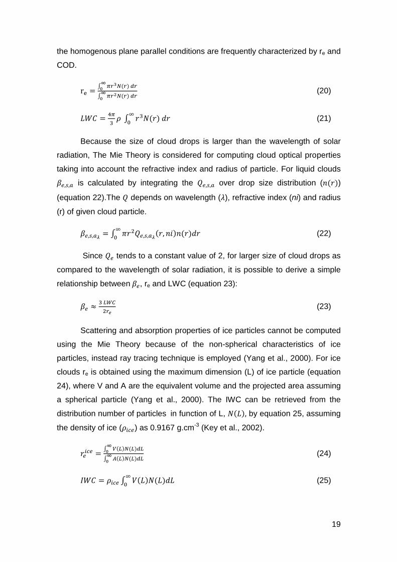
In the Figure 2 the spectral optical properties estimated using the
parameterization developed for liquid clouds (Hu and Stamnes, 1993) and for
rough-aggregated "habit" of ice clouds of Key et al. (2002) are shown. For liquid
clouds, optical properties are presented for re values of 5 µm, 10 µm and 15 µm.
In the case of ice clouds they are computed for re equal to 30 µm, 51.2 µm and
70 µm. Differences of g between clouds are observed, with higher values for
liquid clouds in the spectral range from 0.2 µm up to 1.5 µm (Figure 2.a). Thus,
for the same cloud optical depth, for liquid clouds more forward scattering and
hence a higher transmission of solar radiation is expected as compared to ice
rough-aggregated (near 3D ice) (LeBlanc et al., 2015). However, for plates and
columnar ice particles, g can be higher than for liquid clouds (Key et al., 2002).
Figure 2: Asymmetry parameter (g) (a), single scattering albedo (𝝎) and the ratio between the
extinction coefficient and LWC or IWC (𝛽𝑒 /LWC or IWC) for liquid and ice clouds. For liquid clouds, Hu and Stamnes (1993) parameterization is employed and for ice clouds, the parameterization of Key et al. (2002) for rough-aggregate habit is used. The optical properties are computed for re values of 5,10 and 15 µm for liquid clouds and for 30, 51.2 and 70 µm for ice clouds.
Asymmetry parameter g is sensitive to re (Figure 2.a), while ω near 1
confirms that for clouds, scattering dominates in wavelengths below 1.1 µm.
The absorption of radiation by clouds (ω below 1) is observed for wavelength
higher than 1.1 µm (Figure 2.b) (Marshak et al., 2000). In the solar spectrum,
the extinction coefficient is almost spectrally constant, especially for larger re
(Figure 2.c). 𝛽𝑒 decreases with re and strongly depends on LWC or IWC.
Although 𝑄𝑒 converges to 2 for large size parameter (2𝜋𝐿𝜆⁄ ) also for ice
clouds (Yang et al., 2000), the optical properties of ice clouds depend on the
particle habit. Differences are significant for g in the visible spectrum. Larger ice

21
plates have strong forward scattering with values of g around 0.94. Solid how
columns and bullet rosettes have maximum values of g near 0.86 while for
aggregate, the maximum hardly reaches 0.8. Thus, in the VIS, the R of cloud is
higher (0.65 for COD of 6) for aggregates and solid columns and lower (0.52 for
COD of 6) for ice plates (Key et al., 2002).
The R of clouds is more sensitive to re than T, especially in spectral
regions where the single scattering albedo of clouds is less than 1 (Rawlins and
Foot, 1989). That is because variations of re lead to g and 𝜔 or SSA responses
in the same direction. i. e., the increase (decrease) of re increases (decreases)
the absorption efficiency and forward scattering, contributing to the decrease
(increase) of R. Because of that, retrieving re by measurements of solar
radiation reflected by clouds onboard satellites is more effective (McBride et al.,
2011). At the surface, the opposite behavior of SSA and g causes the less
sensitivity of T to re. In the NIR, larger re results in lower SSA values, reducing
T. The increase of the forward scattering, for larger re, results in the increase of
T. Thus, T measured at the surface in the presence of clouds is more sensitive
to COD than to re (Min and Harrison, 1996). For wavelengths below 1.1 µm, the
higher the re leads to the increase of radiance at zenith due to the direct impact
of the forward scattering. By contrast, for wavelength about 1.4 µm, as the
absorption process becomes more important, the transmitted radiance at
zenith decreases (McBride et al., 2011).
The first works studying cloud and solar radiation interactions focused on
the bulk radiative properties of clouds, i.e reflectivity known as cloud albedo,
absorptivity (the amount of solar radiation absorbed by the cloud layer) and
transmissivity.
One of the first results in the scientific literature about the cloud effects
on solar radiation appeared in the 40’s of the last century (Neiburger, 1949).The
author computed bulk radiative properties of clouds using downwelling and
upwelling shortwave radiation measurements below, inside and above the
coastal stratus clouds in the United States. He showed that the cloud effects
depended on cloud thickness and confirmed, by measurements that the cloud
albedo is the most important property. In addition, low cloud absorption was
22
observed. In that epoch, they argued the need of increasing observations of
cloud microphysical properties.
Paltridge (1974) combined radiative and microphysical measurements
made in stratocumulus clouds. He observed the increase of LWC at high layers
of clouds near the cloud top, with the strong albedo relationship with LWC,
therefore the highest albedo was observed near the cloud top.
Manton (1980) showed the increase of cloud albedo with drops number,
which is higher for thin clouds. Differences were also observed between
maritime and continental clouds, with the continental reflecting 5 % more than
maritime clouds. He also showed the decrease (increase) of reflectivity with re
(LWC). The higher reflectivity near cloud top was strongly related with the
increase of density in this part of the cloud. In addition, the reflectivity
(transmissivity) increased (decreased) for lower CSZA especially lower than
0.5.
Ackerman and Stephens (1987) argued that the scattering properties of
clouds do not depend on droplet size distribution. The cloud absorption
efficiency decreases as an inverse function of re for thin clouds. For deeper
clouds they showed an opposite behavior, with increasing absorption efficiency
for higher re.
2.4.2. Retrieving COD and re from ground based
measurements
Ground-based measurements are useful sources of data to study the
radiative processes in the atmosphere and for validation of satellite
measurements. Around the world, there are still few sites, especially in the
southern hemisphere. A variety of methods for computing cloud optical
properties from passive ground-based measurements has been developed in
the last two decades.
Two approaches for retrieving COD from passive ground-based
instruments are reported in the literature: using broadband or narrowband G,

23
the so called effective cloud optical depth (ECOD) and COD retrieved locally by
using zenith radiance measurements. The former works well for clouds with
total overcast conditions and using 1D radiative transfer model, because the
one to one relationship can be observed between irradiance and COD. In the
case of broken cloud fields, each element of the sky contributes differently to
the irradiance (Marshak et al., 2004), even with enhancement effects, due to 3D
effects of clouds.
Retrieving COD locally has the disadvantage of no one to one
relationship between zenith radiance and COD. Therefore, using combinations
of spectral radiance measurements is needed (Brückner et al., 2014; Chiu et al.,
2010; Marshak et al., 2004). In the following, examples of methods found in the
literature are described.
Leontyeva and Stamnes (1994) proposed the COD estimation from
transmitted irradiance using a broadband pyranometer. They projected a simple
model assuming plane parallel homogenous clouds, without considering the
cloud type or cloud base height. The possible influence of water vapor is not
well represented. They suggested the use of this methodology, but employing a
more accurate model and measurements in the UV and VIS to avoid the
influence of water vapor absorption in the infrared.
Barnard and Long (2004) proposed a simple method for the estimation
of COD using a relationship of COD to G with cases of clouds with total
overcast conditions. They did not consider in depth the atmospheric conditions
for the retrieval; therefore it is less accurate than methods employing spectral
measurements. They also suggested avoiding the use of the method when high
accuracy is needed.
Min and Harrison, (1996) retrieved COD of warm clouds in total overcast
conditions using T415 and surface albedo computed from a Multi-Filter Rotating
Shadowband Radiometer (MFRSR). They also retrieved re from vertical liquid
water path measured by zenith-viewing microwave radiometer (MWR). The
retrieval employed a 1-D radiative transfer model based on the discrete ordinate
method. The advantage of using measurements at channel centered at 415 nm
instead of other spectral regions is argued: the lower surface albedo, the less
24
sensitivity of SSA and g to re and because the absorption of radiation by ozone
in the Chappuis-band can be avoided. COD is retrieved by nonlinear square
method considering cloud properties as stationary in fixed time intervals, by
minimizing the sum of errors in transmittance. The poor ability to distinguish
higher optical depths from satellite measurements at the top of the atmosphere
and the lower uncertainties of retrieving COD from ground-based
measurements were demonstrated.
The best accuracy, close to 5 %, of COD retrieved for thin clouds from
MFRSR was obtained by Min (2004). The method used direct sun irradiance
obtained from MFRSR measurements. A correction for the forward scattering to
avoid underestimation due to the increase of the diffuse contribution in the
direct orientation was developed. The method employed the Bouguer-Lambert-
Beer Law (see equations 10-11) and aerosols can be discriminated from clouds,
using the spectral relationship between the optical depth at 415 nm and 860
nm, with the Ångström exponent (equation 37). It is only applied to thin clouds,
when the direct sun irradiance can be measured.
On the other hand, Marshak et al. (2000) proposed a method for locally
retrieving COD of low broken clouds above green vegetation, using the spectral
contrast of albedo in VIS and NIR for vegetated surface in the presence of low
liquid clouds. COD of clouds is almost constant in the shortwave spectral range.
Therefore in the presence of clouds, radiance at zenith is strongly influenced by
multiple scattering between surface and cloud base. They used the spectral
radiance at 650 nm and 870 nm normalized to the radiance at the top of the
atmosphere. By analogy with the normalized difference vegetation index
(NDVI), they defined the Normalized Difference Cloud Index (NDCI). The NDCI
index minimizes the enhancement effect of zenith radiance due to broken low
cloud fields and shows a good agreement with COD for horizontal resolution
higher than 0.4 km. In addition, the method does not take into account the cloud
fraction, that can lead to poor retrievals.
Based on the relationship of COD with spectral radiance previously
explained, Chiu et al. (2010) proposed a method to compute COD applied to
AERONET measurements, in conditions when aerosol properties cannot be

25
retrieved, called the cloud mode. They used zenith radiance between 440 nm
and 870 nm to take the advantage of more spectral contrast of surface albedo.
This method is effective for low broken cloud fields and it is very sensitive to
aerosol properties, but the authors did not show the errors due aerosols,
arguing that COD retrievals frequently are higher than 15. The total error of the
retrieval is about 17 %, with 4 % due to the re error of 25 %.
McBride et al. (2011) developed a method to retrieve COD and re from
zenith transmitted radiance at 515 nm and the slope of transmitted radiance at
1565 nm and 1634 nm normalized to radiance transmitted at 1565 nm. The
method takes advantage of the variability of spectral absorption efficiency of
clouds in the NIR to obtain the best accuracy for retrieving re. That resulted in
higher sensitivity of the normalized transmittance at NIR to re.
Differences in the shortwave spectral absorption due to the cloud phase was
taken into account by Le Blanc et al. (2015). They derived 15 parameters to
obtain COD, re and cloud phase from spectral transmittance given the cloud
type. But only 2 parameters are derived in the spectral range of VIS, with the
rest in the NIR.
Brückner et al. (2014) retrieved COD and re from 3 ratios of transmissivity
using six spectral ranges (450nm, 680 nm, 1050nm, 1250 nm, 1670 nm, 1560
nm) of zenith radiances. The method is applied to homogenous and
heterogeneous liquid water clouds and cirrus clouds using a 1-D radiative
transfer model. Using combinations of these transmissivity ratios, problems
related to the retrievals of COD lower than 5 were reduced. Errors of retrievals
were near 5 % for low clouds and 10 % for ice clouds, increasing for thicker
clouds.
2.4.3. Computing the shortwave radiative effects of clouds
The shortwave cloud radiative effect (CRE) is a variable that quantifies
the amount of net solar irradiance, or G, affected by the influence of clouds at a
horizontal surface. It can be computed using the 𝐷 ↑𝑐𝑙𝑑 and G (Salgueiro et al.,
2016) in equation 26 or only using G (Tzoumanikas et al., 2016) in equation 26.
In the equations 26 and 28, the subscript clear represents computations under

26
clear sky conditions; usually a radiative transfer model is employed to obtain
this value. The subscript cld corresponds to the irradiances measured in cloudy
conditions. Sometimes 𝐷 ↑𝑐𝑙𝑑 is not measured directly, therefore the use of
surface albedo (𝛼), is needed as shown in equation 27. By the equation 28,
CRE can be computed not including the surface albedo. The CRE is given in W
m-2 and negative values indicate a cooling effect, due to extinction of irradiance
by clouds. Positive values confirm the enhancement effect or the increase of
solar radiation at the surface due to 3D scattering effects by clouds.
𝐶𝑅𝐸 = 𝐺𝑐𝑙𝑑 − 𝐷 ↑𝑐𝑙𝑑− 𝐺𝑐𝑙𝑒𝑎𝑟 + 𝐷 ↑𝑐𝑙𝑒𝑎𝑟 (26)
𝐷 ↑𝑐𝑙𝑑= 𝛼 𝐺𝑐𝑙𝑑 (27)
𝐶𝑅𝐸𝐺 = 𝐺𝑐𝑙𝑑 − 𝐺𝑐𝑙𝑒𝑎𝑟 (28)
The CRE decreases with CSZA and increases with cloud cover
(Tzoumanikas et al., 2016). Other variables are used instead of CRE in order to
minimize the CSZA effect: the normalized cloud radiative effect (NCRE)
(Salgueiro et al., 2016) (equation 29) and cloud modification factor (CMF)
(equation 30). They are variables computed as the ratio of G in all sky
conditions to G in clear sky ones, and they almost totally eliminate the solar
zenith angle effect.
𝑁𝐶𝑅𝐸 =𝐶𝑅𝐸𝐺
𝐺𝑐𝑙𝑒𝑎𝑟 (29)
CMF =𝐺𝑐𝑙𝑑
𝐺𝑐𝑙𝑒𝑎𝑟 (30)
2.4.4. Cloud radiative efficiency (CEF)
To quantify how the cloud radiative effect changes per COD unit, the
cloud radiative efficiency (CEF) is defined. The CEF is computed from the
relationship between the cloud radiative effect and COD. In the case of cloud
with COD below 3 a linear relationship between CRE and COD for any CSZA
are observed, but for higher values of COD an exponential relationship is
expected and CEF is computed from linear relationship between CRE and
ln(COD) for ranges of CSZA (Mateos et al., 2014).

27
In equations 31-33, CEF can be estimated according to Mateos et al.,
(2014) where b is the slope of the relation for different values of CSZA. CEF
computed from CRE has unit of Wm-2 (COD-unit)-1 (Mateos et al., 2014), while
NCRE is in (COD-unit)-1 or % (COD-unit)-1 if NCRE is given in percent values
(Salgueiro et al., 2016).
𝐶𝑅𝐸 = 𝑎 + b ln( 𝐶𝑂𝐷) (31)
𝑏 =Δ𝐶𝑅𝐸
Δ𝐶𝑂𝐷𝐶𝑂𝐷 (32)
𝐶𝐸𝐹 =Δ𝐶𝑅𝐸
Δ𝐶𝑂𝐷=
𝑏
𝐶𝑂𝐷 (33)
CEF is sensitive to CSZA and COD when it is computed from CRE
(Mateos et al., 2014), it increases with CSZA and decreases with COD. Mateos
et al. (2014) showed a maximum efficiency of -160 W/m2 per COD unit at high
CSZA and low COD and minimum of -0.3 W/m2 per COD unit when CSZA is
lower with moderate-large COD. They retrieved COD using broadband
pyranometer measurements with less accuracy, showing a strong relationship
between COD and CRE for a fixed CSZA. In contrast, (Salgueiro et al., 2016)
achieved the best accuracy when CEF was computed based on the linear
relationship between NCRE and ln(COD).
2.4.5. The enhancement effect of clouds on the solar
radiation
In the presence of clouds, if the solar disk is not obstructed, the direct
solar irradiance is not attenuated and the diffuse irradiance can increase. Due
to this effect, called enhancement, the solar G measured at the surface can be
higher than the solar G measured under clear sky conditions keeping all other
variables identical.
The increment of diffuse irradiance is whether can be a consequence of
the multiple reflection of the direct solar irradiance in the border of clouds or the
increase of forward scattering by the cloud (Tzoumanikas et al., 2016). In
special cases, G can overcome an equivalent G at the top of the atmosphere.

28
According to Almeida et al. (2014) these events are called as overirradiance
events.
Tzoumanikas et al (2016) argued that the necessary conditions for cloud
solar enhancement events are: the presence of cumulus clouds, very dense but
not blocking the solar disk, with a minimum value of 50 % and maximum of 90
% cloud cover. These events can last from few seconds to minutes and, in
extreme cases, the measured downward irradiance can be higher than 1500
W/m2 (Tzoumanikas et al., 2016). They observed maximum enhancement of
200 W/m2, occurring in the presence of high and mid-level clouds, values
comparable to low clouds. The position of the solar disk relative to the clouds is
a crucial condition for strong enhancement: solar disk near clouds or low CSZA
with clouds present near zenith (Tzoumanikas et al., 2016). Marín et al. (2017)
showed that the enhancement can be observed at any time of the day CSZA
and the maximum is observed between 40-50 % of cloud cover. They reported
a median of NCRE of 0.18 and percentile 75 of 0.3 at Valencia, Spain.
Enhancement effects at São Paulo were reported before, with the presence of
overirradiance events with time resolution shorter than 1 minute, which were
related to broken cumulus (Almeida et al., 2014).
2.4.6. The shortwave attenuation effect of clouds
The shortwave cooling effect of clouds at the surface is determined when
values of CRE or NCRE are negative. It represents the reduction of solar
radiation at the surface by clouds, as compared to clear sky at the same time.
Tzoumanikas et al (2016) observed maximum of CRE near -900 W/m2
computed with surface albedo. They reported in Greece, strong cooling effects
due to Sc and Cb near -800 W/m2 with CSZA around 0.86. Cu has cooling
effects as high as Sc, but a high variability of CRE was reported with many
cases below -200 W/m2. In the tropical Western Pacific region, Burleyson et al.
(2015) reported the strongest cooling for Cb with NCRE values between -0.81
and -0.84, for low clouds between -0.37 and -0.48, cirrus and mid clouds
presented mean values of NCRE comparable to boundary layer low clouds with
mean between -0.17 and -0.57 and -0.32 and -0.44, respectively.

29
At São Paulo, Yamasoe et al. (2017) reported higher cooling effects
computed using 24 h mean irradiance in summer of -170 Wm-2 and in winter of -
50 Wm-2. They computed mean values of CMF of 0.3 and 0.8 for low and high
clouds respectively.

30
3. Instruments and methods
3.1. Satellite data
3.1.1. Description of satellites
The A-train satellite afternoon constellation is a group of polar orbiting
satellites sharing the same orbit one after another. The time lapse between the
first and the last satellite is only around 15 minutes. Inside this constellation
CALIPSO and CloudSat, launched in 2006, make measurements with intervals
of 15 seconds. The constellation is known as the afternoon due to its overpass
over the equator at 13:30 local time. Near São Paulo, the overpass occurs in
the afternoon around 14:00 LT and near 01:00 LT at night.
CloudSat (acronym of Cloud Satellite) allows estimating the vertical
structure of clouds and precipitation. The main instrument onboard is the
microwave radar with nadir view called Cloud Profiling Radar (CPR) that
measures backscattering from cloud particles at 94 GHz (3.2 mm). The footprint
at sea level has a resolution of 1.7 km and 1.3 km along and across track,
respectively. The vertical resolution of bins is about 240 m and the minimum
detectable radar reflectivity factor is approximately −30 dBZ. Because of the
wavelength of 3.2 mm, CPR of CloudSat is less sensitive to smaller cloud drops
(subvisual cirrus or shallow water droplets), but it can penetrate optically thick
clouds. Moreover, no valid measurements near the surface, specially under 1
km, can be made, due to the backscattering contamination from the surface
(Marchand et al., 2008). The CPR only detects 30 % of clouds under 1 km and
fails in 40 % for retrieving cloud properties due to the limitations of CPR
(Christensen et al., 2013). Since April of 2011, measurements by the satellite
are made only during daytime, because of a battery anomaly.
CALIPSO (acronym of the Cloud-Aerosol Lidar and Infrared Pathfinder
Satellite Observations) satellite has aboard the Cloud-Aerosol Lidar with
Orthogonal Polarization (CALIOP). From CALIOP measurements,
backscattering coefficients at 532 nm and 1064 nm and depolarization ratio at
532 nm are retrieved. The main vertical and horizontal resolutions are 30 m and
333 m, respectively up to 8.2 km, and from 8.2 km until 20 km the vertical and

31
horizontal resolutions are 60 m and 1 km respectively (Winker et al., 2009).
With CALIPSO, smaller cloud drop such as from sub visual cirrus or
semitransparent clouds of boundary layer, can be detected. Hence, the synergy
of radar and lidar is very powerful because the constraints of each instrument
on detecting clouds are minimized.
3.1.2. CloudSat and CALIPSO products
In this research, microphysical variables for liquid clouds are obtained
from 2B-CWC-RO products of CloudSat. The data can be downloaded in the
following website: http://www.cloudsat.cira.colostate.edu/). In addition, because
of this product also has profiles for liquid clouds available, cloud properties such
as cloud thickness can be estimated for low clouds.
For ice clouds, properties are obtained from CSCA-Micro of JAXA
products (http://www.eorc.jaxa.jp/EARTHCARE/research_product/ecare_monito.html).
Cloud particle definition from CA-Ctype was used to estimate the frequency of
habit for layer and for clouds. Cloud mask of lidar/radar from CSCA-Cmask was
employed to compute the geometric properties cloud base for liquid and ice
clouds and thickness for ice clouds. Cloud frequency by height level was also
obtained for each season and according to distance from the coastal line. The
coastal line distance was estimated as the minimum distance of the
measurement point to the coast. The computations of frequency of occurrence
are valid if at least 100 measurements were found in every layer, or every bin
selected of coastal distance.
The time period of 2B-CWC-RO spans from December 2007 to June
2016 with a total of 436 overpasses. Quality control was made neglecting
measurements under precipitation and uncertainties above 20 %. In addition, a
total of 382 overpasses were found in JAXA products in the full period between
July 2006 and August 2015. In the following, the methodology of retrieving each
product is briefly described.
3.1.2.1. CloudSat

32
Liquid water content (LWC), ice water content (IWC), effective radius (re)
are included in the Cloud Water Content using Radar Only product (2B-CWC-
RO) from CloudSat products. The retrieval algorithm uses at first a cloud mask
from 2B-GEOPROF product to detect the layer with presence of clouds (Mace,
2007). Later, it employs 2B-CLD-CLASS product where cloud types are defined
and allows for checking if a level previously classified as cloudy is undetermined
or invalid which indicates troubles in the vertical profile of clouds (Austin, 2007).
The algorithm assumes the entire profile with ice or water clouds.
Finally, microphysics properties are retrieved using a forward scattering
model using a priori information of size distribution of drops. The model
considers lognormal size distribution depending on three parameters. In
addition, the radar reflectivity, LWC/IWC and re are related with the same three
parameters. Thus, the final retrieval is made by iteration from a priori
information up to the convergence of the solution (Austin, 2007). The algorithm
underestimates re and LWC/IWC in the presence of precipitation, dBZ>-15,
because it does not consider the size distribution of precipitating drops (Austin,
2007). Christensen et al. (2013) showed the high uncertainty in the retrieval for
mixed-phase profile due to the erroneous selection of refractive index. 2B-
CWC-RO has a horizontal resolution of 1.1 km with 125 vertical levels of 240 m
each.
3.1.2.2. CloudSat-CALIPSO (JAXA products)
Recently, a synergy between CALIPSO-CloudSat was publicized by the
EarthCARE Research Product Monitor of Japan Aerospace Exploration Agency
(JAXA), where between others, microphysics properties of ice clouds, a new
cloud mask and cloud type particle or habit of ice clouds are available. Products
of JAXA Radar/Lidar Cloud Mask Product (CSCA-Cmask), Lidar Cloud Particle
Type Product (CA-Ctype) and Radar/Lidar and Cloud Microphysics Property
Product (CSCA-Micro) were employed in this research.
CSCA-Cmask includes a new cloud mask from merged CALIPSO-
CloudSat cloud masks. This new cloud mask developed by Hagihara et al.
(2010) incorporated and improved cloud mask from CALIPSO and cloud mask
from 2B-GEOPROF of CloudSat. They applied two criteria for defining a cloudy

33
bin: the first considering a threshold of total attenuated backscattering
coefficient at 532 nm, the second one, a continuity test. The continuity test is
based on grouping bins along track into a two dimensional space and a new bin
is considered cloudy if at least half of pixels in the space are considered cloudy
by the first criterion.
The improved cloud mask from CALIPSO better classifies the clouds as
compared to the vertical feature mask (VFM) from original CALIPSO datasets;
especially for low clouds over dust. The new CALIPSO-CloudSat cloud mask
improves the CloudSat mask, especially for cloud tops below 720 m above the
ground (Hagihara et al., 2010).
CA-Ctype includes phase and type of cloud particle. Yoshida et al. (2010)
developed a method for discriminating cloud particle type based on the
relationship between depolarization ratio and ratio of backscattering coefficient
between two consecutive layers (X). It is based on the fact that liquid drops
have values of depolarization ratio as higher as for the case of ice drops, but
differences are found for X, because it is proportional to the first layer optical
depth. Discrimination based on temperature is also considered. The following
cloud particles types are considered: 3-D ice, 2-D plate, warm water and
supercooled water.
Cloud microphysics properties such as re for ice clouds and IWC are
included in CSCA-Micro product. The combinations of radar-lidar for retrieving
microphysics properties are more accurate than only using Radar (Okamoto et
al., 2010). Thus, re and IWC are retrieved by using lookup-tables where radar
reflectivity (Ze), depolarization ratio and attenuated backscattering coefficient
are the input variables. In the retrieval, specular reflection is taking into account
improving the accuracy of the method for cases with presence of 2-D plates
(Okamoto et al., 2010). The method is also applied for only radar or lidar cloud
mask, but input variables that cannot be measured are inferred from
relationships previously computed in the overlap radar-lidar layers in the same
profile.
The A-train trajectory does not overpass the campus USP (23.56° S,
46.73° W). The nearest overpass occurs at a minimum distance of 25 km with

34
the maximum frequency of overpasses near 75 km. Therefore, data from
overpasses distant at maximum 100 km from the ground site were selected.
3.2. Ground based measurements
At IAG meteorological station, far away 15 km to the Campus USP,
visual observations are made along with variables of weather conditions
measurements. Moreover, on the top of the Pelletron building (30 m height
above ground surface) at the Instituto de Fisica da Universidade de São Paulo
(IF-USP) in the Campus USP, three instruments are installed: sun-photometer
from CIMEL, model CE318, Multifilter Rotating Shadowband Radiometer
(MFRSR) from Yes Inc., and a broadband pyranometer from Kipp & Zonen,
model CM21. Furthermore, nearby at Center for Lasers and Applications (CLA)
of the Nuclear and Energy Research Institute, a total sky camera and Raman
lidar are also running continuously.
3.2.1. Visual observations of clouds1
At IAG meteorological station (23,65° S, 46,61° W, 800 m a.s.l) with a
since 1957, clouds are reported by human visual observations every hour from
7:00 Local Time (LT) up to 0:00 LT. A total of 12 cloud types are reported:
fractocumulus (Fc) and fractostratus (Fs), along with 10 main cloud types
defined by the World Meteorological Organization (WMO). In addition to cloud
type, the cloud amount (cloud cover) at each height level (low, middle and high)
is also reported (in tenths). This cloud amount is reported from a surface
reference point; and the sum of the cloud amount reported at each level
reaches a maximum of 10 tenths.
3.2.2. Pyranometer
The pyranometer measures G at the surface, integrated from 305 nm up
to 2800 nm, with a time resolution of 1 minute. It is provided with a thermal
detector where energy is absorbed and converted to voltage. Measured units
1 This section is part of Datasets and Methods of a paper submitted to the International
Journal of Climatology, ID=JOC-18-0083, for possible publication.

35
are converted to W m-2 using a calibration factor. It is calibrated about every two
years at LIM (Laboratório de Instrumentos Meteorológicos from Instituto de
Pesquisas Espaciais - INPE). Database of pyranometer measurements spans
from January 2016 until September 2017.
3.2.3. Multifilter Rotating Shadowband Radiometer (MFRSR)
Aside the pyranometer, two MFRSRs, numbered 345 and 368, make,
simultaneous measurements every 1 minute. The MFRSR measures 𝐺𝜆, 𝑆𝑆𝜆,
and 𝐷 ↓𝜆, at 5 narrowband channels centered at wavelengths: 415 nm, 670 nm,
940 nm, 870 nm, 1036 nm. It has an automatic band that blocks the sun
allowing to measure 𝐷 ↓𝜆. The 𝑆𝑆𝜆 is retrived from the difference between 𝐺𝜆
and 𝐷 ↓𝜆 using the CSZA as shown in the equation 17. In addition, the
instrument has a broadband silicon detector which measures global and diffuse
irradiance in the spectral range from 300 to 1100 nm.
The MFRSR 345 narrow band channels are calibrated every two years;
thus, spectral corresponding values at the top of the atmosphere (TOA) are
estimated. A total of 118523 measurements were made with this instrument,
spanning only 6 months of data from September 2016 up to February 2017.
Data from instrument 368 were employed for radiative computations and cloud
properties retrievals, since it was running from June 2012 until September 2017.
There are some measurement gaps for MFRSR 368: December 2012,
January 2014, from May to September 2014, November 2014, January 2015
and from April to July 2015. To calibrate MFRSR 368, coincident measurements
with MFRSR 345 were used, as will be detailed in section 3.5.2.
3.2.4. AERONET sun-photometer
Sun-photometer CIMEL, model CE318, is an automatic sun/sky spectral
radiometer with 1.2 ° field of view (FOV) which measures direct sun and sky
radiance in spectral narrow bands. The instrument placed in the site of USP
campus USP (23.56 °S, 46.73 °W) has 8 spectral bands centered at 340 nm,
380 nm, 440 nm, 500 nm, 675 nm, 870 nm, 940 nm, and 1020 nm. Direct sun
measurements are carried out in the eight bands. AOD (except at 940 nm) and

36
precipitable water vapor (at 940 nm) are retrieved from inversion methods using
spectral direct sun irradiances applying the Beer-Lambert-Bouguer law. It
returns to NASA Goddard Space Flight Center facility every two years for
calibration purposes.
Sky radiance measurements are employed for retrieving other properties
of aerosols e.g. size distributions, asymmetry parameter and single scattering
albedo (Dubovik and King, 2000). The surface albedo is also obtained by
combination of sky radiance and TOA measurements made by satellites
(Sinyuk et al., 2007). Spectral surface albedo is given at 440 nm, 670 nm, 870
nm and 1020 nm using Moderate Resolution Imaging Spectroradiometer
(MODIS) data, at or near the channels the of sun-photometer.
COD is retrieved from radiance measurements made at zenith at 440 nm
and 870 nm, in conditions where direct sun measurements are impossible to
make due to obstruction of sun disk by clouds (Chiu et al., 2010). The
methodology is better detailed in section 2.4.3. Since November of 2000 sun-
photometer is working at the site retrieving aerosol properties. COD began to be
retrieved in May 2016. Measurements of sun-photometer are made each 15
minutes, but in some cases around sunrise it is reduced to 5 minutes.
For AOD, there are 3 quality levels: level 1.0 which is not cloud screened,
1.5 for cloud screened and 2.0 for cloud screened and post calibration. In the
case of COD, there are two levels: 1.0 and 1.5. For COD, at level 1.0, the
retrieval is made by using climatological values of surface spectral reflectance
and for COD level 1.5, the spectral surface reflectance is obtained from MODIS
measurements. COD are retrieved every 15 min if clouds are present, while
each measurement takes about 1.5 min.
For this research, the following variables from sun-photometry were
used: spectral AOD, Ångström exponent, SSA, g, surface albedo, COD and
precipitable water vapor. In addition, ancillary information on NO2 and O3
column integrated data was also employed. Data were downloaded from the
site: https://aeronet.gsfc.nasa.gov/ .
3.2.5. Sky camera

37
At Center for Lasers and Applications (CLA) of the Nuclear and Energy
Research Institute (IPEN) (Latitude: -23.56°: Longitude: -46.74°, 740 m above
sea level), total sky camera J1006 is working since August 2016.
The camera is a weatherproof automatic system that captures cloud
cover with a fisheye lens. It has a resolution of 4M pixel and includes a
processor to perform digital images. Moreover, a powerful “Find clouds”
software allows to classifying the clear sky, total hemispheric cloud cover,
optically thick and thin clouds, direct sun detection and cloud cover of the free
and above artificial horizon.
In this research, regular pictures each 5 min were used from August
2016 to September 2017. Images can be obtained in the website:
http://gescon.ipen.br/leal/10-1.Measurements-2018.html .
3.2.6. Lidar
In the CLA of IPEN, since 2001, there is a multiwavelength Raman Lidar
installed. The fundamental emission is made at 1064 nm and additional
emissions at 532 and 355 nm are made using second and third harmonic
generators. The detection and spectral selection is made in the following
wavelengths: 1064 nm, 532 nm and 355 nm, 607 nm, 387 nm, 408 nm (da Silva
et al., 2017).
In this research, backscattering coefficient profiles of measurements at
532 nm were employed for around two days for each month of clear sky
conditions observed in 2015. A fixed value 60 of aerosol lidar ratio is assumed
and the profile defined between 300 and 6000 m above ground. Aerosol
extinction coefficient profiles from the system were employed.
3.3. Methodology of cloud climatology from visual
observation2
Cloud amount reported from visual observations per height level does not
represent the actual cloud cover for mid or high clouds when they are present
2 This section is part of Datasets and Methods of a paper submitted to the International
Journal of Climatology, ID=JOC-18-0083, for possible publication

38
with lower clouds. In order to infer the amount of clouds when they are hidden
by lower clouds or mid and lower clouds, a random overlap assumption (Tian
and Curry, 1989) is applied and shown in equation 34. The terms i and i-1 are
the current level and the level below it, respectively, N is the cloud cover or
cloud amount in the respective level. When high clouds are present with mid
and low clouds, cloud cover of the underlying level is the sum of cloud cover of
low and middle level clouds reported by the observer.
The real cloud cover NiR can be estimated with a maximum of 7/10 of the sky
obscured by underlying level clouds. With the presence of a Cumulonimbus
cloud (Cb) this equation is not employed due to the weakness of the
relationship (Tian and Curry, 1989).
NiR =
Ni
(10−Ni−1)∙ 100 (34)
For this research, only daytime (7:00-18:00 LT) cloud data were analyzed
due to restrictions to observe clouds at night. Observations from 1957 up to
2016 were considered, spanning a total of 59 years.
Cloud occurrence frequency (fq) for each cloud type is computed as the
ratio between the number of cases of each cloud type reported at a given height
level and the total number of cloud observations in that level. For mid and high
clouds, the height level is observable and considered viable if there is at least 3
tenths of the sky free of clouds to make sure that clouds are observable. This
condition is very important for high level clouds, because in several occasions,
the presence of lower clouds does not allow to observe possible higher clouds,
which consequently are not reported, producing underestimated frequency
values.
Cloud amount when cloud is present (awp) is the mean of cloud cover
computed when a cloud type is reported alone at a particular height level. Mean
cloud amount (amt), is the mean cloud cover computed, and for each cloud type
can be estimated from frequency and awp (equation 35). Values of awp are
converted to percent values for better analysis.
amt(%) = fq ∙ awp(%) (35)

39
In addition to the frequency of occurrence, co-occurrence frequency
(frequency of occurrence of one cloud type given another cloud type) is
computed. This variable symbolizes the dependence of one cloud from other
clouds. The most important cloud combinations by observed frequency were
also specified.
Trend of cloud amount is represented as the slope of a linear fit of mean
annual cloud amount as function of year, with statistical significance computed
with the modified Mann-Kendall Test (Hamed and Rao, 1998) at a significance
level of 5 %. Trend value is reported as %/ decade. Special emphasis is made
for diurnal cycle and it is analyzed in depth, computing phase and amplitude.
The phase was computed as the hour of maximum cloud cover and the
amplitude as the difference between maximum and mean cloud cover
computed for each day. Also, mean diurnal cycles for every 15 days along the
year were computed.
3.4. Radiative transfer model (uvspec from LibRadtran)
LibRadtran is a library containing programs and routines of radiative transfer
in shortwave and longwave spectra. The radiative transfer program uvspec, in
the shortwave spectrum, with 1-D configuration of LibRadtran version 2.0, was
employed in this study to compute downward solar irradiance reaching the
surface. The discrete ordinate method (disort) with 6 streams was selected as
the radiative transfer solver of the program (Stamnes et al., 1988).
The REPTRAN band parameterization (Gasteiger et al., 2014) with spectral
resolutions of 15 cm-1 was the adopted molecular absorption parameterization.
Trace gases, pressure and temperature profiles from the standard tropical
atmosphere (Anderson et al., 1986), where the atmosphere is divided in 50
levels from surface up to 120 km, were chosen. O3 and NO2 were modified from
the initial profile by using monthly mean values of total column concentrations.
O3 total column concentration given in Dobson units (DU) was obtained from
Total Ozone Mapping Spectrometer (TOMS) (McPeters et al., 1998) and
downloaded from: https://ozoneaq.gsfc.nasa.gov/. NO2 total concentrations in
molec/cm2 (Boersma et al., 2004) were obtained from ESA Scanning Imaging
Absorption Spectrometer for Atmospheric Chartography (SCIAMACHY), at:
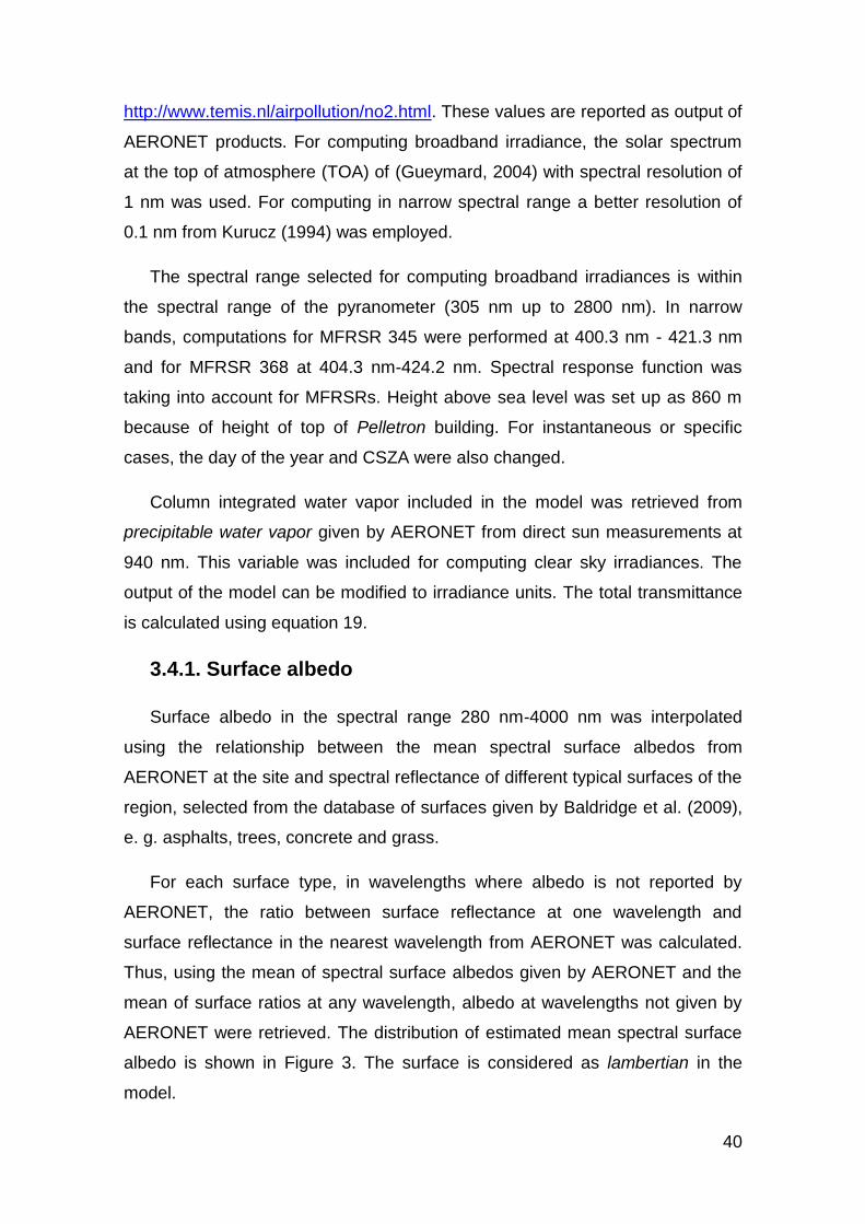
40
http://www.temis.nl/airpollution/no2.html. These values are reported as output of
AERONET products. For computing broadband irradiance, the solar spectrum
at the top of atmosphere (TOA) of (Gueymard, 2004) with spectral resolution of
1 nm was used. For computing in narrow spectral range a better resolution of
0.1 nm from Kurucz (1994) was employed.
The spectral range selected for computing broadband irradiances is within
the spectral range of the pyranometer (305 nm up to 2800 nm). In narrow
bands, computations for MFRSR 345 were performed at 400.3 nm - 421.3 nm
and for MFRSR 368 at 404.3 nm-424.2 nm. Spectral response function was
taking into account for MFRSRs. Height above sea level was set up as 860 m
because of height of top of Pelletron building. For instantaneous or specific
cases, the day of the year and CSZA were also changed.
Column integrated water vapor included in the model was retrieved from
precipitable water vapor given by AERONET from direct sun measurements at
940 nm. This variable was included for computing clear sky irradiances. The
output of the model can be modified to irradiance units. The total transmittance
is calculated using equation 19.
3.4.1. Surface albedo
Surface albedo in the spectral range 280 nm-4000 nm was interpolated
using the relationship between the mean spectral surface albedos from
AERONET at the site and spectral reflectance of different typical surfaces of the
region, selected from the database of surfaces given by Baldridge et al. (2009),
e. g. asphalts, trees, concrete and grass.
For each surface type, in wavelengths where albedo is not reported by
AERONET, the ratio between surface reflectance at one wavelength and
surface reflectance in the nearest wavelength from AERONET was calculated.
Thus, using the mean of spectral surface albedos given by AERONET and the
mean of surface ratios at any wavelength, albedo at wavelengths not given by
AERONET were retrieved. The distribution of estimated mean spectral surface
albedo is shown in Figure 3. The surface is considered as lambertian in the
model.

41
3.4.2. Aerosols
Vertical profiles of aerosol particles were built using extinction coefficient
computed from backscattering coefficient at 532 nm measured by ground-based
Lidar. For each clear sky day, morning and afternoon mean profiles of extinction
coefficient were normalized with respect to the mean AOD computed by
integrating the extinction coefficient in the column, hereinafter called AODlidar.
Owing to values of extinction coefficient were retrieved only above 300
m, it was essential to know what fraction of total AOD was below 300 m. In
order to compute the contribution of AOD below 300 m, mean AOD from sun-
photometer (AODAERONET) in the same time interval of LIDAR was subtracted
from the mean AODlidar as long as AODAERONET was higher than AODlidar. Then,
a mean ratio between AOD from the lowest layer of LIDAR relative to AOD
below 300 m was calculated. AOD below 300 m was included in the mean
profile using the former ratio.
Figure 3: Mean spectral surface albedo used as input in the uvspec radiative transfer model.
Due to the lack of clear annual trend of stratospheric AOD in the last
decade, a mean value of stratospheric AOD of 0.008 was taken into account in
the computations (Vernier et al.,2011).
In figure 4.a, normalized extinction coefficient profiles from LIDAR, for
each season and part of the day, are shown. Note the maximum near 300 m
and the seasonal and diurnal differences. In the mornings, as expected,

42
aerosols are more concentrated near surface as compared to the afternoon,
when loading of aerosol increases aloft. Remarkable increase is observed
above 2 km due to the advection of biomass burning aerosols in spring (SON)
(de Miranda et al., 2017). With the aim of including aerosols in the radiative
transfer model, the normalized AOD profiles (𝐴𝑂𝐷𝑁𝑂𝑅𝑀(𝑍)) below 8 km
including AOD below 300 m were grouped in two seasons: typical: when
profiles of the spring are not included, characterizing mean local contributions
and spring (SON): mean profile for spring season, with advection of biomass
burning plumes. Profiles were also classified as morning and afternoon.
Figure 4: Mean profiles of normalized aerosol extinction coefficient for each season and time of the day (a) and the normalized profile of AOD built by synergy between LIDAR and sun-photometer for normal or typical conditions and for conditions with biomass burning plume advection in spring (SON) (b).
The spectral AOD profile included in the uvspec model was constructed
using the profile of normalized AOD and values of AOD retrieved by AERONET
(equation 36).
𝐴𝑂𝐷 (𝜆, 𝑍) = 𝐴𝑂𝐷𝐴𝐸𝑅𝑂𝑁𝐸𝑇(𝜆) ∙ 𝐴𝑂𝐷𝑁𝑂𝑅𝑀(𝑍) (36)
Narrowband irradiance around 415 nm was computed using AOD415,
estimated with AOD440 and the empirical formula of Ångström (equation 37),
using the exponent (𝛼) determined with the 380 nm and 440 nm AOD values
retrieved by AERONET.

43
For broadband computations, AOD at 500 nm was employed and
spectral dependence was included using the Ångström exponent 𝛼 and
Ångström’s turbidity coefficient (𝛽) (equation 37). This method has a good
accuracy as reported by Serrano et al. (2014). SSA mean values of 0.85 and
0.90 were assumed (de Almeida Castanho et al., 2008), for local conditions and
during spring time respectively.
𝐴𝑂𝐷(𝜆) = 𝛽𝜆−𝛼 (37)
Under cloudy conditions AOD is not retrieved by sun-photometry,
therefore four methods for estimating AOD at MFRSR 415 nm channel and
pyranometer were developed:
Time interpolation of AOD throughout the day;
Adjust climatological monthly diurnal cycle from at least one AOD
retrieved on the same day;
Adjust climatological monthly diurnal cycle of AOD from mean diurnal
AOD computed as near as at least 2 days;
Climatological monthly diurnal cycle of AOD.
Error in the estimation of AOD and contribution of error to COD retrieval by
each method will be analyzed and discussed in section 4.3.2.1.
3.4.3. Clouds
Ice and liquid clouds were included in the model and assumed as
homogenous layers. Cloud base and top, mean re and mean LWC/IWC are the
input variables for clouds. These inputs were assumed from microphysical and
geometric properties obtained from CALIPSO and CALIPSO-CloudSat as
explained before. In table 2, the default configurations for each cloud type are
summarized. Analysis of variability of cloud properties from satellite retrieval is
carried out in section 4.1.
The parametrization used for liquid clouds is given by Hu and Stamnes
(1993), where COD is obtained from re and LWC. They showed that the shape
of the cloud droplet size distribution does not affect the results (re represents

44
well the drop size distribution of clouds). This parametrization is as accurate
and faster in computation time than from Mie theory.
For ice clouds, the employed parametrization was from Key et al. (2002)
where optical properties of seven shapes of ice particles (habits) are
parametrized depending on re and IWC. According to the selected habit,
differences can be as higher as 15 %, especially between ice plate and the
other habits. The habit selected is the Rough Aggregated as an example of 3D
ice. In section 4.1 the selection of this habit is discussed.
Table 2: Default cloud configuration assumed in the radiative transfer code.
Cloud Top (km) Base (km) re (µm) LWC/IWC (g/m
3)
Ice 10.05 9.09 51.2 0.01 Liq. 1.60 0.86 11.6 0.23
3.5. Methodology of the radiative computations and COD
retrieval.
In the figure 5 the flow chart of the procedures for the retrieval of COD
and radiative effects computations are shown. The main datasets are the global
irradiance measured by the pyranometer and spectral diffuse and direct
irradiances at 415 nm and 870 nm measured by the MFRSR. Three steps
before the direct computations with LibRadtran are carried out. First, the 1 min
instantaneous calibrated measurements of MFRSR and Pyranometer are time-
collocated with precipitable water vapor and AOD from sun-photometer. The
second step is the definition of cloud scenarios by the Sky Definition method,
detailed in the next section. After the measurements are filtered, the mean
aerosol profiles according to the season and hour, in combination with the
coincident AOD from sun-photometer, are used as input in the radiative transfer
model. In addition, the mean microphysical properties retrieved from the
combination of CALIPSO-CloudSat, for ice and liquid clouds are inputted to the
model used in the retrieval of ECOD.

45
Figure 5: Flow chart of the main procedures carried out for the ECOD retrieval and computations of cloud radiative effects.
3.5.1. Sky definition
Ancillary information concerning cloud presence and obstruction of solar
disk are needed to classify the measurements made by pyranometer or
MFRSR. Because the time period of all sky-camera is limited (started in
September 2016), before this date, algorithms to define the presence of clouds
were required. Therefore three algorithms were developed for applying in
absence of sky camera observations: using visual observations of clouds,
spectral ratio of diffuse irradiance. In addition, algorithm of obstruction of solar
disk by clouds was defined. If the three algorithms were coincident, the
instantaneous measurements were classified. In the following the three
algorithms are detailed.
3.5.1.1. Sky definition by visual observations
Time coincidence with visual observations in a time window of 20
minutes before and after the time of observation was a criterion selected to

46
classify the sky by visual observations above the measurement site. Despite the
distance from the site is about 15 km in a straight line to the meteorological
station where visual observations are made, we considered that the spatial
variability in clouds between the two sites were not as high as to make
significant differences in cases when clear sky or total cloud cover were
reported.
Comparing with observations from the sky camera, with 6868 cases of
total overcast conditions, 99.68 % of coincidence was found with visual
observations from the meteorological station, when cloud cover greater or equal
9 tenths was observed. Below 8 tenths, a 100 % of coincidence were noted.
Thus, visual observation can be a useful ancillary data in dates when sky
camera observation was not available. For clear sky conditions, more than 95 %
of data observed as clear sky by the sky camera were reported also at the
meteorological station.
Classification of sky from visual observations is as follows:
Clear sky, if the maximum of cloud cover is 20 % with no presence of
high clouds.
Low/mid/high cloud partially overcast: only low/mid/high clouds with
cloud cover below 70 %.
Low/mid/high clouds total overcast: only low/mid/high clouds with cloud
cover of 100 %.
3.5.1.2. Direct sun criterion (solar disk obstruction)
In addition to cloud cover, information about obstruction of solar disk is
needed. With MFRSR measurements direct sun irradiance can be derived.
Then, comparisons of Tdir modeled for clear solar disk by uvspec and measured
Tdir at 415 nm were also used to classify the conditions of the solar disk. Min,
(2004) screened clouds by using direct sun irradiance when thin clouds were
present by applying threshold of Ångström exponent for aerosols. But it is only
limited to thin clouds and needs to compute spectral AOD with MFRSR which is
beyond the scope of this research.

47
The solar disk was considered obstructed by cirrus clouds when
modeled Tdir was 15% higher than the Tdir measured, otherwise it was
considered as a clear disk. This threshold was selected after the analysis of
uvspec error in computing Tdir at 415 nm for clear sky conditions (section 4.3.3).
The 15 % difference criterion works better for cirrus clouds with lower
COD values, but in the case of low clouds, with the presence of interstices, it is
not robust. Therefore to avoid misclassification in low clouds conditions,
differences between Tdir modeled for clear sun disk and Tdir measured must be
higher than 200 %. For mid-level clouds, 20 % of difference was considered.
These thresholds were stablished analyzing cases observed by the sky camera.
3.5.1.3. Spectral diffuse ratio (DR)
The presence of clouds can modify the spectral distribution of diffuse
radiance relative to ones of clear sky. The physical reason is that cloud drops
are larger than molecules and aerosols; therefore they present lower spectral
dependence in the solar extinction, i. e., compared to aerosols and molecules.
Thus a ratio between diffuse irradiance at 870 nm and 415 nm hereinafter
diffuse ratio (DR) can be a good indicator of the presence of clouds.
This ratio is based on the method applied by (Min et al., 2008) using the
diffuse transmittance to compute cloud fraction. Furthermore, LeBlanc et al.
(2015) employed the spectral ratio of radiance at zenith at 870 nm and 600 nm
measured at the surface. They showed the high sensitivity of the ratio at lower
CODs.
In figure 6, the variation of DR with CSZA, COD for cloudy and AOD500
for clear sky is evaluated using 1-D uvspec model. AOD500 was varied between
0.08 and 0.8. Between 0.08 and 0.3 the step was 0.03, while above 0.3 it was
equal to 0.1. COD for ice clouds spans from 0.03 up to 4, with steps of 0.5, and
for liquid clouds, it varied between 3 and 100, with steps of 5.As it can be
observed in the figure 6, DR varies between cloudy and clear skies. Below
AOD500 of 0.3, clear sky can be distinguished from sub visual cirrus with COD of
0.03. When single scattering dominates over multiple scattering, the sensitivity
with CSZA is observed. That can be noted for clear sky and for low COD of ice

48
clouds. When multiple scattering dominates DR is less sensitive to CSZA (low
clouds and higher COD of ice clouds). From the behavior observed for low
clouds is possible to clearly identify them over the clear sky cases. But
differences between ice and liquid clouds are not so obvious for thick cirrus
clouds.
Figure 6: Variations of diffuse ratio, at channels 870 nm and 415 nm, at surface level, with CSZA and AOD for clear sky, and COD of ice and liquid clouds computed from 1-D uvspec model of LibRadtran. The darker the color the higher the value of AOD500 or COD. COD for ice clouds spans from 0.03 up to 4 and, for liquid clouds, it varies between 3 and 100. AOD500 is varied between 0.08 and 0.8. Between 0.08 and 0.3 the step is 0.03, while above 0.3 is 0.1.
From the aforementioned analysis of DR, it is possible to make a criterion
to define clear and overcast sky, using spectral measurements of diffuse
irradiance from MFRSR. Therefore, after validation using real measurements
(section 4.3.4), the following criteria are used to define cloudy and clear sky:
Clear sky (clear) is defined when AOD500 is below 0.30, because above
0.30 can be overlapped with subvisual cirrus. Therefore depending on
CSZA for AOD below 0.3 clear sky cases can be defined by the
expression given in the equation 38.
𝐷𝑅 < 2.8 ∙ 10−2 ⋅ 𝐶𝑆𝑍𝐴−2 − 0.11 ∙ 𝐶𝑆𝑍𝐴 + 0.25 (38)
Total overcast sky, with high/mid-level clouds (mid or high overcast), is
defined by the equation 39, where coefficients a, b and c depend on
AOD500, to avoid overlap with possible clear sky.

49
𝐷𝑅 > 𝑎 ⋅ 𝐶𝑆𝑍𝐴−2 + 𝑏 ∙ 𝐶𝑆𝑍𝐴 + 𝑐 (39)
Total overcast sky with low cloud, mid or high clouds (low, mid or high
overcast) is classified if DR is above 0.6.
After the coincidence between the three methods (in the Sky definition),
before September 2016, 110727 cases for MFRSR 368 were classified
according to cloud scenarios shown in table 3. A total of 59592 of total overcast
sky cases, including low and high clouds, were employed to retrieve ECOD. For
pyranometer measurements, 26853 cases were classified.
In Table 3, a resume of sky definition algorithms to define cloud scenario
are shown. For the ECOD retrieval, cloud scenarios LW_0 and H_0 were
employed. For cloud radiative effects all the scenarios were used. Note, that
after September of 2016 only definition of visual observation from sky camera
pictures and direct sun criterion are employed.
Table 3: Sky definition algorithm for the clouds scenarios defined in this research.
Sky definition Cloud scenario Visual Direct sun DR
Low clouds total overcast obstructed Low overcast LW_0
Low clouds partially overcast obstructed Not clear LWBK_0
Low clouds partially overcast clear Not clear LWBK_1
High clouds total overcast obstructed High overcast H_0
High clouds partially overcast obstructed Not clear HBK_0
High clouds partially overcast clear Not clear HBK_1
Mid clouds total overcast obstructed Mid overcast MID_0
Mid clouds partially overcast clear Not clear MIDBK_1
3.5.2. Calibration of MFRSR 368
Transmittance from MFRSR 368 at 415 nm is the main input variable to
be used for retrieving the effective cloud optical depth. This instrument was
calibrated using indirect calibration (Holben et al., 1998). The idea is to transfer
the calibration of MFRSR 345 to MFRSR 368 using coincident measurements
under clear sky conditions. Cases of clear sky were selected from sky camera
after September of 2016. An inverse method from Lambert-Beer equation was

50
applied, using the AOD at 415 nm computed from MFRSR 345. Retrieval of
AOD415 from MFRSR was carried out by the same method applied by Sayão,
(2008).
The aim of the calibration procedure is to obtain the equivalent solar
irradiance at 1 astronomical unit (AU) (𝑆𝑆0) at TOA (equation 40). Where 𝑆𝑆𝑠 is
the direct sun irradiance measured at surface, 𝑘 is the correction factor of Earth-
Sun distance, 𝑚 is the relative optical air mass for Rayleigh scattering,
𝑀𝑂𝐷 𝑎𝑛𝑑 𝑁𝑂𝐷 are the molecular optical depth due to Rayleigh scattering and
nitrogen dioxide, respectively. 𝐴𝑂𝐷415345 is the aerosol optical depth at 415 nm
retrieved from MFRSR 345.
𝑆𝑆0 = 𝑘−1𝑆𝑆𝑠 exp[𝑚(𝐴𝑂𝐷415345 + 𝑀𝑂𝐷 + 𝑁𝑂𝐷)] (40)
For every 1 min of clear sky data, 𝑆𝑆0 was retrieved and time
interpolations were made for measurements with no clear sky conditions. For
cases when time interpolation was impossible to make, the nearest neighbor
interpolation was carried out. After calibration, T was computed using equation
18.
3.5.3. The retrieval of effective cloud optical depth
Since cloud optical depth was obtained from hemispherical
measurements under total overcast conditions, the term Effective Cloud Optical
Depth (ECOD) can be adopted. The retrieval of ECOD was carried out by
inversion method using 𝑇𝑡 at 415 nm computed from measurements of MFRSR
368. Transmittance was selected because errors associated to the calibration
accuracy were reduced. At around 415 nm, surface albedo is low, thus multiple
scattering between surface and cloud base is minimized. In addition, at this
wavelength there is only weak NO2 absorption and O3 absorption is negligible.
Furthermore, there is no spectral variability of COD at these wavelengths (Min
and Harrison, 1996). As the retrieval was applied for total overcast conditions,
and the model did not allow the inclusion of clouds with mixed phase, the
retrieval method was applied for either low (warm phase) or high clouds (ice
phase).

51
Visual observation with sky camera helped classifying total overcast
cases after September of 2016. Before this date, the sky definition criterion
(section 3.5.1) was applied. Cases under precipitation were discarded using the
report of precipitation made at the meteorological station.
Based on the method applied by Salgueiro et al. (2016), but including the
aerosol effect, lookup-tables (LT) for each cloud type (ice or liquid) were built
using the 1-D uvspec where output is 𝑇415.The input variables of each LT are:
CSZA, AOD415, COD and aerosol profile. The aerosol profile (figure 4.b) was
selected depending on season and time of the day. The sensitive study is
carried out in section 4.3.1, and the selection of input variables is discussed.
The procedure to retrieve COD is discussed as follows:
First, the aerosol profile is selected, afterward 2D cubic interpolation of
𝑇415 depending on CSZA and AOD415 for each COD step is carried out,
i.e. 𝑇415 =f(AOD415, CSZA). Therefore, 𝑇415 is estimated from the measured
AOD415 and CSZA for every COD step. Subsequently, linear interpolation of
estimated 𝑇415 as function of COD is computed. Using the linear interpolation,
ECOD is retrieved as the minimum difference between 𝑇415 estimated and 𝑇415
measured by iteration along the COD values.
In the configurations of each LT, AOD415 varied between 0 and 1.5 and
CSZA between 0.1 and 1 with steps of 0.05. For liquid clouds, COD varied from
0 up to 400 with step of 1. In the case of ice clouds, COD varied from 0 up to
40, with steps between 0 and 4 of 0.25 and 1 above 4.
3.5.3.1. Error in COD retrieval
The error propagation for COD retrieval is expressed in equation 41, as
the root square of the sum of error squared of each variable i. The relative error
is computed as the ratio of each error and the COD value retrieved.
𝛿𝐶𝑂𝐷 = [∑ (𝜕𝐶𝑂𝐷
𝜕𝑖𝛿𝑖)
2
𝑖 ]
1
2 (41)
Applying the methodology proposed by Serrano et al. (2014) (equations
42-44) the contribution of each variable to the COD error is retrieved. The

52
variation of T due to the error of variable i assuming the other variables constant
is 𝛿𝑇𝑖. In addition, the variation of T due to the possible error induced in COD
(𝛿𝐶𝑂𝐷𝑖) is 𝛿𝑇𝑐𝑜𝑑. Differences between 𝛿𝑇𝑖 and 𝛿𝑇𝑐𝑜𝑑 are computed by iteration
of 𝛿𝐶𝑂𝐷𝑖. When the difference between 𝛿𝑇𝑖 and 𝛿𝑇𝑐𝑜𝑑 is the minimum, 𝛿𝐶𝑂𝐷𝑖 is
obtained. The computation of T is carried out using the uvspec considering
CSZA equal 0.86.
𝜕𝐶𝑂𝐷
𝜕𝑖𝛿𝑖 ≈ 𝛿𝐶𝑂𝐷𝑖 (42)
𝛿𝑇𝑖 =1
2|𝑇(𝑖 + 𝛿𝑖, 𝐶𝑂𝐷) − 𝑇(𝑖 − 𝛿𝑖, 𝐶𝑂𝐷)| (43)
𝛿𝑇𝑐𝑜𝑑 =1
2|𝑇(𝑖, 𝐶𝑂𝐷 + 𝛿𝐶𝑂𝐷𝑖) − 𝑇(𝑖, 𝐶𝑂𝐷 − 𝛿𝐶𝑂𝐷𝑖)| (44)
Because of the transmittance error is directly related to the error
associated to the calibration procedure, 2 % of error is assumed. For single
scattering albedo, the error of retrieval from sun-photometer is about 0.05
(Dubovik et al., 2000), since the error decreases to 0.03 for AOD440 above 0.20
and around 0.05-0.07 for AOD below 0.20. SSA mean values of 0.85 and 0.90
were assumed (de Almeida Castanho et al., 2008), for local conditions and
during spring time, when biomass burning plumes are transported to the city,
respectively. The error of assuming mean value of SSA is the standard
deviation of SSA obtained from sun-photometer at the site. Therefore the total
error of SSA (𝛿𝑆𝑆𝐴), including the error of the retrieval is 0.19.
For AOD, the error assumed is the sum of error of AOD measurement
(0.02) (Serrano et al., 2014) and the maximum error of inferring AOD, from
mean monthly diurnal cycle at 415 nm (0.11) (Table 6). The standard deviation
of samples of cloud properties was assumed as the cloud properties errors. For
ice clouds error of re (𝛿𝑟𝑒) is about 40 µm and for low clouds, 2 µm. For cloud
base error (𝛿𝐶𝐵) it is computed as 2.8 km and 2.7 km for ice and liquid clouds,
respectively. The results of error propagation are presented in section 4.3.2.
3.5.4. Instantaneous cloud effects on solar radiation
The instantaneous cloud effect on solar radiation was evaluated by CRE
and NCRE (equations 26 and 29 of chapter 2). Irradiances measured every 1

53
min from pyranometer were selected as cloudy conditions, while irradiance for
clear sky was estimated using uvspec model.
Default configuration, explained in the topic 3.4, was used to calculate
irradiance under clear sky conditions. As will be discussed in the next chapter
(Results), in general, the model overestimated clear sky irradiances compared
to the measurements. The maximum relative difference of 15% and 5 % was
observed for overestimation and underestimation, respectively. To avoid
erroneous estimation of the cloud effect on solar radiation, when the relative
difference between modeled and measured irradiance was higher than – 5 %
and less than 15 %, the case was discarded.
For solar disk blocked by clouds, the following cases (according to table
3) were analyzed: completely or total overcast sky with low clouds (LW_0),
partially overcast with low clouds (LWBK_0), total overcast sky due to high
clouds (H_0), partially overcast sky with high clouds (HBK_0) and total overcast
sky due to mid clouds (MID_0). When the solar disk was clear, the following
cases were computed: low clouds (LWBK_1), high clouds (HBK_1) and mid
clouds (MIDBK_1).

54
4. Results
4.1. Cloud characteristics from CALIPSO-CloudSat
Seasonal profiles of frequency of occurrence of clouds for nighttime
(01:00 LT) and afternoon (14:00 LT) overpasses are shown in figure 7. There
were more than of 2000 profiles measured at night and more than 7000
measured in daytime for each season. Seasonal and day/night differences are
clearly observed.
Figure 7: Profiles of frequency of occurrence of clouds per season at nighttime (a) and daytime (b), computed from cloud mask generated by merged CALIPSO-CloudSat data.
Higher frequencies of clouds were observed in summer, whose vertical
development could reach 17 km. In winter, lower frequencies were found and
clouds could reach 15 km. The contrast between daytime and nighttime profiles
is observed. In daytime profiles the maximum frequency, around 30 %, takes
place near 2500 m in summer. As a consequence of the diurnal heating, cloud
frequency increased at lower layers during daytime. At night, cloud frequency
decreased a little below 2 km, and increased at mid (7.5 km) and high layers
(12 km) with 35 % of frequency in summer, as a consequence of the remaining
convective activity in the afternoon. At night, convection tends to disappear and
the water vapor supply from surface decreases, low clouds begin to evaporate
until radiative cooling starts the formation of stratiform low clouds (Wood, 2012).

55
In mid and high layers, clouds remain due to the weak circulation and the
radiative cooling which maintains or increases the clouds.
At daytime, from summer to winter, the decrease of cloud frequency is
observed more pronounced at lower layers from about 32 % to 14 %. At
nighttime higher differences are found in higher layers from 35 % to 5 %. In
winter, the maximum frequency is observed in lower layers with 15 % at
nighttime and minimum in higher layers. This maximum in lower layers at
nighttime is a consequence of the increase of radiative cooling.
In the figure 8, profiles of cloud frequency as function of the distance
from the coast are presented. In the computations, measurements at nighttime
and daytime were used together. Variability is also observed as the distance
from the coast line increases.
Figure 8: Frequency of presence of clouds relative to the distance from the coast line.
Note near the coast up to 20 km the convection activity is expected to be
less strong compared to inland. With a distance below 20 km far from the coast
line, the maximum frequency at lower layers (2.5 km a.s.l) with 26 % is
observed. From the edge of Serra do Mar mountain barrier (from 20 km) an
increase of cloudiness in mid and high layers is observed with maximum

56
frequency near 50 km from the coast, with 24 % frequency of occurrence near
10 km of height.
While the distance to the coast increased, low clouds frequency begin to
decrease and an increase of the height of clouds and frequency is observed.
Maximum of cloud frequency was found 100 km away from the coast and near
12 km height with 32 %. Undoubtedly, this behavior illustrates that convective
clouds are more frequent inland.
Geometrical properties, cloud base height and cloud thickness for ice
and liquid clouds for each season are shown in figure 9. Moreover, the number
of identified clouds is also shown above of each boxplots. In the case of cloud
base of warm clouds a slight variability is observed, with similar values for the
median in all seasons, but, in winter, heights of cloud base are more
concentrated around the median with the smallest interquartile range. However,
hypothesis test of Kruskal-Wallis (Kruskal and Wallis, 1952) does not show
differences between seasonal samples. Cloud base of liquid clouds at the
region presents the median value of 860 m.
Figure 9: Seasonal variations of geometrical properties of clouds: the height of base and thickness of liquid clouds (a, b) and ice clouds (c, d). The number of clouds identified is also shown in the upper border of each figure.
As expected, in summer, warm clouds are deeper with median of 900 m.
In winter and spring, the median of cloud thickness is around 600 m. For ice
clouds differences are larger, cloud base is higher in summer with a median of

57
11 km, and lower in winter (9.5 km). According to Kruskal-Wallis H-test,
differences are statistically significant. The thicker of ice clouds in winter,
probably has to do with the lower cloud base.
The seasonal variability of microphysical properties for ice and liquid
clouds is shown in figure 10. Liquid clouds show small sizes as compared to ice
clouds. Seasonal differences with statistical significance between re of liquid
clouds re confirmed by the Kruskal-Wallis H-test. The highest value of the
median occurs in winter with 11.8 µm, because in this season clouds are more
frequently originated from interaction of cold air mass outbreaks and sea, as a
result of cold migratory anticyclone systems.
Figure 10: Microphysics properties re and LWC or IWC for liquid (a, b) and ice clouds (c, d). For liquid clouds, the products of CloudSat are employed and for ice cloud, CSCA-Micro product was considered. The number of cases is placed in the upper border of each figure.
Similar to re, LWC has differences with the highest median in winter, but
with the minimum observed in spring. For ice clouds, the seasonal differences
are smaller with many outliers for effective radius, above 200 µm, while the
median values are around 51 µm. The general median value, considering all
data available, is equal 51.23 µm. IWC also presented many outliers with values
higher than 0.5 g /m3, with some values comparable to the maximum LWC
observed for low clouds, although the median presented little seasonal
differences with values around 0.01 g /m3.

58
To try to know the more frequent particle habit in the region, the product
of JAXA CA-Ctype for cloud particles was used. The frequency of occurrence of
cloud particle habit per height level for each season is presented in figure 11.
Three types of habit were analyzed: 3D-ice (3dic), 2D-plate (2dpl) and
mixture of 3D-ice and 2D-plate (mx3i2p). The predominance of three
dimensional ices is observed specially above 10 km where almost 100 % of ice
cloud layers are composed of it. In addition, 2D-plate habit is more frequent in
mid-levels particularly between 6 and 8 km with higher frequency in autumn and
winter probably due to the weaker updrafts (Heymsfield et al., 2017) as
compared to summer and spring. At 4 km to 8 km there is higher variability of
habit being impossible to define a fixed classification.
Figure 11: Profiles of frequency of occurrence of ice cloud habit for each season (a) and frequency of occurrence of cloud layer totally composed by a given cloud particle habit.
The frequency of occurrence of cloud habit is presented in figure 11 b. In
the region, clouds are predominantly composed by 3D ice particles with 95 % of
frequency, followed by the mixture of 3D with 2D plates with 4 % frequency and,
in the case of only 2D plates; they were identified in 1 % of data only. After this
analysis, the type of habit chosen as input in the uvspec of LibRadtran code for
ice clouds was the one with 3D geometry (as example 'Rough Aggregated').
Variations of microphysics properties inside the ice clouds respect to the
height above the cloud base are shown in figure 12.a-b. Median values and
interquartile ranges are presented. As it can be seen, ice clouds are far from
and idealized homogenous cloud. The decrease of cloud particle sizes and ice

59
water content is observed with the height above cloud base. The re can
decrease from 60 µm up to 40 µm near cloud top. But for IWC the reduction is
higher from near 10 mg m-3 until 2 mg m-3 near the top of cloud. This pattern is
a response to the decrease of water vapor availability as the temperature
decreases with the height.
Variations of mean microphysical properties of all cases of clouds
respect the height of cloud base are shown in figures 12 c-d. Mean re decreases
as cloud base is higher from 6 km (102 µm) up to 12 km (40 µm). However,
near 13.5 km a slight increase is observed. For IWC this behavior is also
observed with a higher increase near 13.5 km which can be attributed to cirrus
from remaining storms.
Figure 12: Variations of re and IWC with height above cloud base (a, b) and variations
of mean re and IWC of the cloud layer according to the height of cloud base (c,d).
4.2. Cloud climatology from visual observations3
4.2.1. Diurnal and annual cycles of cloud amount
3 This section is part of Results of the paper submitted to the International Journal of
Climatology, ID=JOC-18-0083, for possible publication.

60
Figure 13.a shows the mean diurnal cycle and respective variability of
clouds amount from visual observations. Figure 13.b-c gives indication of the
associated annual variability, i.e. how the hour of maximum and amplitude of
diurnal cycle vary along the year.
Figure 13: Mean diurnal cycle and standard deviation (a) computed from mean diurnal cycles calculated for every 15 days. Variability of the diurnal cycle for every 15 days computed as hour of maximum (b) and Amplitude (c).
The mean total cloud amount (clouds) decreases after sunrise until
about 11:00 LT (63 %), with a monotonically increase with the advance of the
day up to a maximum at sunset (74 %). This behavior is initially associated with
the possible increase of cloud amount in the end of the night, due to radiative
cooling. After sunrise, the radiative cooling is surpassed by solar heating,
breaking the inversion layer above cloud, and dissipating the cloud layer. The
posterior increase after 11:00 LT is due to convective development caused by
the solar heating, influence of the sea breeze or a synoptic system. If
convection is deep, formation of high and mid-level clouds are possible. High or
mid-level clouds, formed by convection, remain or increase in cloud amount at
night driven by radiative cooling (Heymsfield et al., 2017). Hence, mid and high
clouds present an inverse diurnal cycle of cloud amount as compared to solar
heating diurnal cycle (figure 13.a.).

61
This diurnal cycle of clouds is variable along the year (Figure 13.b-c),
with the maximum observed at sunset from September to March and around
sunrise from April to August. The decrease observed near sunrise (Figure 13.a)
takes longer in wintertime and lasts two hours more (until about noon)
compared to summer (not shown in figure). Undoubtedly, differences along the
year were due to differences of driven mechanism of cloud formation. In winter,
radiative cooling dominates, there is less deep convection and air humidity is
reduced, whereas in summer, deep convection is more frequent.
Low clouds drive the diurnal cycle of clouds as can be observed by the
similarity in their cycles. Low clouds has a significant influence of low stratiform
clouds, since they are the more abundant type of clouds in the location, and
only a pronounced increase in the diurnal cycle at noon and a slightly decrease
near 16:00 LT are due to cumuliform clouds.
Note the differences between low stratiform and cumulus clouds.
Stratiform clouds are less influenced by the solar cycle, rather the radiative
cooling effect is responsible for the formation at night and sunrise (Wood,
2012). When isolating low stratiform clouds (not shown), it is possible to
observe that the maximum cloud amount occurs for stratus clouds at sunrise
and for stratocumulus at sunset, thus, from Figure 13.b, maximum of diurnal
cycle probably can be influenced because stratus prevails in winter, while
stratocumulus dominates during the summer season. It is important to observe
that other mechanisms can lead to the formation of stratiform clouds, not only
radiative cooling, particularly in summer and spring, as will be discussed later.
This behavior was not observed when analyzing the synoptic reports (Eastman
and Warren, 2014) because of the underestimation of Sc when they are present
with Cb. Moreover in the region, there can be an important contribution of
cumulonimbus clouds by the possible influence of the sea breeze circulation,
synoptic systems as SACZ and cold fronts. The amplitude of stratiform clouds
was less variable along the year with maximum in autumn-winter (Figure 13.c),
and minimum in April. In this month, the increase of cloud amount at sunset is
less pronounced and the radiative cooling at sunrise is negligible, producing
lower amplitude in the diurnal cycle. In addition, in this month, cold fronts are
highly frequent (Morais et al., 2010).

62
Cumulus clouds, by contrast, present high dependence on the solar
heating diurnal cycle, with maximum near noon, throughout the year (Figure
13.b). Furthermore, this maximum occurs two hours later in winter compared to
summer. That is because, in winter, the maximum of cloud cover is found at
sunrise leading to delaying of surface heating by solar radiation, thus, the
increase of cloud amount by convection can start only in the afternoon. Note the
differences in amplitude of cumulus along the year, with the highest amplitude
in summer of about 15 % and minimum in winter, near 5 %.
The maximum amplitude, above 15 %, is also observed in summer for
mid-level clouds. Mid and cirriform clouds show comparable characteristics with
maximum in spring-summer at sunset, except on the first 15 days of October
when the maximum is observed at 7:00 LT. In autumn-winter, one observes a
maximum of mid clouds at sunrise but, for cirrus, the maximum can take place
near sunset. Note that, for cirrus, from January to March, the maximum is
observed in the morning.
Figure 14: Mean annual cycle computed for every 15 days. The vertical bars represent the inter-annual variability.
The annual cycle, computed every 15 days, is shown in Figure 14. Mean
values and standard deviation are presented. Observe the seasonal variability
for total cloud cover (clouds) with a minimum in early August. Maximum takes
place in summertime, between December and January. Low clouds show

63
minimum in the first part of August but, in contrast to total cloud cover, an
increase is observed between March and April due to the same increase
detected in this period for stratiform clouds. As mentioned before, the peak of
cold front systems crossing the region, as diagnosed by Morais et al. (2010),
can contribute to this increase.
Cirriform clouds presented less contrast between winter and summer,
with differences of about 15 %, with the maximum observed in spring, in late
October of 35 %. Mid-level clouds have a maximum of amt in the beginning of
January (40 %) and minimum on the first 15 days of August with 17 %.
Cumuliform clouds have an observable seasonal behavior with differences
between winter and summer of 18 %. The maximum is observed in the end of
December with 20 % and the minimum on the last 15 days of September (2%).
4.2.2. Inter-annual variability of cloud amount
The inter-annual variability of cloud amount is analyzed in this section.
Seasonal mean values are shown in Figure 15 for the six main cloud
categories. Seasonal variability and trends are observable especially for low
stratiform and mid-level clouds. Low clouds have an increasing trend due to the
stratiform variability. This increase is observable from the second half of 1980’s.
Total cloud amount (Clouds) has not a clear trend in any season, with
maxima of annual means occurring in summer. Absolute maximum and
minimum of total cloud amount is perceived in summer of 1975 (87.7 %) and
winter of 1963 (42.7 %), respectively. For mid-level clouds, a decrease after
1990 in all the seasons is evidently observed. The maximum occurred in
summer of 1965 (53.2 %) and minimum in winter of 2010 (1.9 %). Conversely,
cirriform clouds presented a slight increase especially in summer with maximum
observed in summer of 2010 (41.4 %) and minimum in winter of 1964 (7.4 %).
Furthermore, low clouds presented a maximum in spring of 2005 (70.1 %) and
minimum in winter of 1972 (25.2 %). In the same years, the maximum and
minimum of stratiform clouds were observed, with 71.7 % and 24 %,
respectively.

64
Figure 15: Mean values of cloud cover (amt) per year computed for every cloud type in summer (a,b ), autumn (c,d ), winter (e,f), spring (g,h).
Cumuliform clouds presented the maximum in summer of 2001 with an
absolute value of 24 % and minimum in winter of 1995 with 0.5 %.
Trend values computed as the slope of linear regression are shown in
Table 4. We estimated annual trends and for each season separately. Bold
values indicate trends that are statistically significant at 5 % confidence level.
These values were computed for the total time interval and for the first and last
30 years.
Table 4: Seasonal and annual trends (%/decade) computed for each cloud type, in three different time intervals. Statistical significance was computed by the modified Mann-Kendall Test at 5 % of confidence level and they are highlighted in bold.
Cloud Type
PERIOD TIME 1958-2016 1958-1988 1987-2016
DEF MAM JJA SON Total DEF MAM JJA SON Total DEF MAM JJA SON Total
Low 2.0 1.8 1.0 1.8 1,6 -0,1 0,5 -0,6 1,0 0,2 4,4 4,1 2,3 2,3 3,2
Mid -3.1 -2.2 -1.6 -2.7 -2,4 -0,3 2,2 0,5 -1,3 0,3 -7,3 -5,3 -3,1 -4,8 -5,2
Cirr 1.0 1.1 0.4 0.7 0,8 2,3 1,9 2,1 0,0 1,6 2,2 2,2 0,2 2,4 1,7
Str 3.7 3.5 2.0 3.0 3,1 5,9 5,7 2,1 5,0 4,8 1,5 2,2 1,3 0,8 1,3
Cu -0.1 -0.5 -0.5 -0.3 -0,3 0,1 0,3 -0,4 0,2 0,1 0,7 0,0 0,2 0,2 0,2
Clouds 0.2 0.8 0.1 0.4 0,4 0,8 2,3 1,2 0,3 1,1 0,1 1,2 0,3 0,4 0,6
From 1958 to 1988 an increasing trend is observed, but only with
statistical significance in all seasons for stratiform low clouds. For cirriform
clouds, statistical significance is observed in winter (2.1 %/decade) and for all

65
the year with 1.6 %/decade. For total cloud cover only in autumn an increase
was observed (2.3 %/decade).
After 1987 the increasing trend is higher for low clouds (3.2 %/decade)
due to a little increase with no statistical significance of Cu and stratiform low
clouds. In addition, it is noteworthy the decrease observed for mid-level clouds
in all seasons, with trend with annual mean values of about -5.2 %/decade. In
addition the increase of cirriform clouds of 1.7 % was noted in this period time.
For the total period of study, from 1958 to 2016 the decrease in mid-
level clouds amount in all the seasons with statistical significance is observed.
The maximum decrease of about -3 %/decade was found in summer. Cirriform
clouds showed a positive trend with significance in an annual basis (0.8
%/decade) and in autumn (1.1 %/decade). Cumuliform clouds presented a
decreasing trend with statistical significance, except for summer. But low clouds
increased in all seasons (above 1 %/decade) as a consequence of the highest
increasing trend observed for low stratiform clouds (above 2 %/decade) in all
seasons.
Comparing trends computed for a grid near the region for daytime data
by Eastman and Warren (2013) for the period 1971-2009, differences in low
cloud cover were found. While they reported a decreasing trend, it is clearly
noted an increasing trend of low clouds in this study. These differences are due
to stratiform clouds, because in this study a significant increasing trend was
observed for all season, whereas for Eastman and Warren (2013) a minor
increase was only observed in summer and autumn. Moreover, low cumuliform
cloud trends showed the best agreement between both studies, with reduction
in all seasons.
Trends of high and mid-level cloud almost agreed, presenting higher
decrease in our study. Differences in trends were only observed in summer for
mid-level clouds and spring for high clouds. For the total cloud cover trends,
similar results were found, except for spring and summer when positive trends
were observed in this study, but with no statistical significance.

66
Seasonal trends at distinct local time are shown in Table 5. It is clearly
observed a decrease for mid-level clouds during daytime hours in all seasons
with maximum decrease at sunrise. The absolute maximum occurred in spring
during sunrise (-3.8 %/decade). Low and stratiform cloud amounts were
increasing in the afternoon with maximum at sunset, except in winter, when
maximum trends occurred around noon, while cumuliform clouds showed
decreasing trend near noon, except during summer. Cirriform cloud amount
increased in sunrise and midday, but with statistical significance around noon
for autumn, spring and in the annual basis, and around sunrise in summer. For
total cloud cover, an increasing trend of 0.8 %/decade around noon and a
decreasing trend of -0.5 %/decade at sunrise were observed on an annual
basis. In autumn, cloud cover showed increase after midday and decrease at
sunrise.
Table 5: Trends (%/decade) of 6 six clouds types computed for sunrise (7 SLH), noon (13 SLH) and sunset (18 SLH). Statistical significance was computed by Mann- Kendall Test in 5 % and they are in bold.
Cloud Type
DJF MAM JJA SON Total
7 SLH
13 SLH
18 SLH
7 SLH
13 SLH
18 SLH
7 SLH
13 SLH
18 SLH
7 SLH
13 SLH
18 SLH
7 SLH
13 SLH
18 SLH
Low 0,4 2,6 3,4 -0,1 2,8 3,5 0,6 1,2 1,0 0,6 2,2 2,6 0,4 2,2 2,6
Mid -3,5 -3,1 -3,3 -3,3 -1,8 -3,1 -2,5 -1,4 -2,1 -3,8 -2,2 -2,7 -3,2 -2,2 -3,0
Cirr 1,3 0,7 -1,0 1,2 1,4 0,1 0,9 0,2 -0,2 0,6 1,1 0,6 1,1 0,8 -0,2
Str 0,6 6,2 4,2 0,0 6,5 3,7 0,7 2,8 1,3 0,7 4,6 2,9 0,5 4,9 3,0
Cu 0,1 0,4 0,2 0,1 -1,1 0,2 0,1 -1,0 0,0 0,2 -0,7 0,2 0,1 -0,6 0,1
Clouds -0,4 0,6 0,2 -0,7 1,7 1,2 -0,2 0,1 -0,4 -0,5 0,9 0,6 -0,5 0,8 0,4
4.2.3. Simultaneous occurrence and combinations of clouds
Following the methodology applied by Warren et al. (1985), in this
section, the simultaneous occurrence of cloud types is analyzed. Table 6 shows
cloud frequency of occurrence and cloud frequency of co-occurrence (cloud
type occurrence given another cloud type) for each season. In this case, Cu,
Sc, St, Cb, Ac, Ns and Cirriform clouds were employed. As can be seen, almost
all cloud types presented maximum frequency in summer except for stratus
clouds, whose maximum was observed in spring. In this season, the frequency
of cold front passage in the region is high, with 27 % of events of the year
(Morais et al., 2010).

67
Table 6: Frequency of occurrence and co-occurrence for clouds types for each season
Given
cloud
season Fq Frequency of occurrence due to given cloud type
Cu Sc St Cb Ac As Ns Ci
Cu
DJF 40.7 - 56.8 0.9 4.4 32.3 14.5 0.0 46.8
MAM 33.2 - 58.3 1.2 1.8 21.5 6.1 0.0 31.8
JJA 13.9 - 54.1 0.9 0.3 14.9 2.9 0.0 25.9
SON 22.7 - 55.9 0.9 1.6 21.4 7.7 0.0 34.9
Sc DJF 57.4 23.1 16.2 3.4 43.5 33.8 0.1 48.3
MAM 51.9 19.4 16.3 1.4 32.5 18.7 0.0 33.9
JJA 33.8 7.5 23.7 0.2 25.4 14.3 0.0 28.6
SON 49.2 12.7 24.5 1.0 32.8 25.0 0.0 36.1
St DJF 16.1 0.3 57.7 2.0 34.8 67.1 0.0 52.5
MAM 17.2 0.4 49.4 0.9 29.4 39.8 0.1 35.4
JJA 20.6 0.1 39.0 0.2 23.3 32.4 0.0 28.9
SON 25.4 0.2 47.6 0.6 30.3 54.8 0.1 40.3
Cb DJF 3.2 1.8 59.6 9.7 54.1 48.1 0.5 61.6
MAM 1.2 0.6 61.1 12.8 46.3 44.7 0.0 62.1
JJA 0.1 0.0 58.8 35.3 54.8 45.2 0.0
SON 0.9 0.4 52.9 15.3 48.4 42.4 0.5 67.2
Ac DJF 40.1 10.0 46.8 2.5 2.8 41.0 0.0 69.6
MAM 28.2 5.8 45.6 3.1 1.2 31.2 0.0 57.0
JJA 18.6 1.8 28.4 2.7 0.2 28.6 0.0 51.1
SON 27.6 3.9 38.7 3.4 1.1 41.2 0.0 61.8
As DJF 24.8 4.5 58.8 7.9 4.0 66.2 0.1 89.4
MAM 13.2 1.6 55.9 8.9 2.4 66.6 0.0 88.3
JJA 7.9 0.3 38.1 9.0 0.4 67.8 0.0 86.9
SON 17.2 1.4 47.2 9.8 1.5 65.9 0.1 89.6
Ns DJF 0.1 0.0 30.3 0.0 12.1 12.1 39.4
MAM 0.0 0.0
JJA 0.0 0.0
SON 0.0 0.0
Ci DJF 51.7 11.5 33.1 1.1 1.8 31.0 8.1 0.0
MAM 36.8 7.5 32.7 1.8 0.9 24.5 5.1 0.0
JJA 32.8 2.9 16.1 1.3 0.1 16.7 3.4 0.0
SON 38.3 5.6 26.4 1.5 0.8 21.9 5.5 0.0
Likewise, it is noticeable the Sc maximum in summer in contrast with the
global studies of Warren et al. (2007) and Wood (2012). However, it is important
to keep in mind that the Metropolitan Area of São Paulo (MASP) is located over
a plateau of 800m above sea level and close to the coast (about 50 km in
straight line).

68
Due to the parallel orientation of the mountain range to the coast line,
mountain-valley circulation contributes to the advance of sea breeze inland. In
addition, circulation generated by the urban heat island effect makes the sea
front to be stationary at MASP. This phenomenon influences the local
circulation and, acting isolated or with other systems, contributes to many cases
of floods in the region (Freitas et al., 2009). From the analysis of wind direction,
Perez and Silva Dias (2017) found that the sea breeze reaches the city earlier
in summer and spring (around 14:00 LT), compared to the other seasons.
In summer and spring the early arrival of the breeze is associated to the
higher contrast between the ocean and land surface temperatures. The
conditions are most favorable due to the increase of the land temperature and
the position of the South Atlantic high pressure. The breeze front can contribute
to the formation of convective clouds along with a composite of clouds such as
stratocumulus. Besides, possible advection of low stratiform clouds formed near
the coast and in the edge of the mountain barrier can occur. Note that more
than 50 % of Cb cases were in the presence of stratocumulus in all seasons.
Conversely, cumuliform clouds frequency, when Cb was present, was near null.
Dynamic processes associated with Cb can be another forcing mechanism for
stratocumulus development in the area. Downdraft outflow from Cb can lead to
the formation of other low cloud types, by means of formation of gust front
(Mahoney, 1988). This was not reported in previous studies using synoptic
reports, probably because of the constraint mentioned before related to the
presence of Cb and the way of synoptic observations were carried out.
It is also significant the higher dependence of mid-level and cirriform
clouds on cumulonimbus. Observe that cirrus is present with almost all cloud
types, with especially higher frequency with presence of As, Ac and Cb.
Likewise, note how Sc and Ac are related especially in summer, once Ac can
form from ascending layers of stratocumulus clouds.
For the analyzed period, 536 combinations of clouds were found; the top
10 by frequency of occurrence for each season are shown in the Figure 16. As
can be observed, there is an evident predominance of stratiform cloud
combinations except for Cu-Ci, Ci and Cu. The highest frequency was found for

69
Sc with maximum of about 16 % in spring. Maxima frequency are also observed
in spring for combinations with stratiform clouds; in summer for the combination
with cumuliform clouds; and, in winter, for Ci and Ac. Mean cloud cover when
the combination is present (awp) is shown in Figure 15.b. Observe the higher
values for St, Sc-St, Sc-Ac and Sc-Ac-St. Minima of awp were observed for Ci
and Cu with 50 % and 45 %, respectively.
The diurnal cycle of the first 8 combinations is shown in Figure 17.
Combinations of stratiform clouds show an inverse diurnal cycle compared to
combination with cumuliform clouds. At sunrise, the highest frequency for
stratus combination is observed. Also, Sc showed increase in the morning with
maximum near 9:00 LT. Observe the maximum frequency of cirrus-only at
10:00 LT, following the decrease observed for low cloud cover. Around noon
Sc, Sc-Cu and Cu were predominant. At sunset Sc has the highest frequency
followed by stratus clouds. Observe, in the figure 17.b, that cloud cover, when
combinations are present, is higher throughout the day for low stratiform
combinations, and the influence of the solar heating cycle on cloud cover of
cumuliform combinations is also noted.
Figure 16: Mean frequency of occurrence (fq) and sky cover when present (awp) for the12 main cloud combinations observed at each season.

70
Figure 17: Diurnal cycles of the 8 main combinations of clouds for frequency of occurrence (a) and amount when present (b).
4.3. Sensitive study for COD retrievals
4.3.1. Sensitive of properties at 415 nm
To build the lookup tables for COD retrievals using T, a sensitivity
analysis of T to changes in some variables was needed. Variations of T at 415
nm modeled by uvspec to variations of surface albedo, aerosol vertical profile,
SSA, g, AOD, gas concentrations and cloud properties are analyzed in this
section. The sensitivity of each variable was carried out by changing the
variable between percentiles 5 and 95 % according to measured data, while
keeping the others constant. Values of COD were assumed constant equal 2 for
ice clouds and 10 for low clouds. Default model configuration (section 3.4) is
used with CSZA of 0.86, AOD415 with 0.3, SSA415 assumed from SSA440 with
0.81 and g 415 assumed from g440 with 0.7.
Variations of T415 with respect to aerosol properties are presented in
Figure 18. The effect of the four aerosol profiles, retrieved from ground-based
measurement of Lidar and sun-photometer at the site, is compared with the two
profiles given by the LibRadtran library, labeled summer-spring and winter-
autumn (Mayer et al., 2015). It is clearly observed the little sensitivity of T to the

71
different aerosol profiles (Figure 18.a). But differences about 1.5 % were found
between the typical profile and the profile for spring.
Figure 18: Sensitivity of transmittance at 415 nm for liquid and ice clouds to variations of aerosol vertical profile [mo_ty= morning typical, mo_sp= morning in spring, af_ty=afternoon typical, af_sp=afternoon in spring, su-sp=summer-spring and au-wi=autumn-winter given by LibRadtran (Mayer et al., 2015) (a), variations of AOD415 (b), variations of SSA440 (c) and g440 (d).
In the case of variations of AOD415 (Figure 18.b) changes were observed,
especially for ice clouds, for which T415 decreased linearly with slope of about
21.5 % per AOD415 unit. For low clouds, there is less sensitivity to aerosol load
of about 8.3 % per AOD unit.
The SSA440 also influenced the T415 (Figure 18.c), the increase of SSA440
contributed to the increase of scattering and hence T415 was higher. Between
percentile 95 and 5, the differences of T were about 7 % for liquid and ice
clouds. The variation of T between 5 % and 95 % of g440 obtained from
AERONET products was almost imperceptible (Figure 18.d). Differences
between the extreme values of g440 were 0.6 % and 0.1 % for ice and low
clouds, respectively.
The sensitivity of T415 to CSZA was higher (Figure 19 a), especially for
ice clouds, between 95 % and 5 % percentiles, the difference can reach more

72
than 100 %. For surface albedo, NO2 and O3 there is no perceptible variation
(Figure 19).
Figure 19. As in the Figure 16 but for CSZA (a), surface albedo at 415 nm (b), dioxide of nitrogen (NO2) (c) and ozone (O3) (d).
Figure 20. Variations of total transmittance at 415 nm to cloud base, thickness, re and LWC for ice and liquid clouds with a constant value of COD.
Sensitivity of T415 to cloud properties is shown in Figure 20. For liquid
clouds, T415 varied around 2 % with the height of cloud base between
percentiles 5 and 95 %. Note the lower variability to re of ice and liquid clouds.
For high clouds, and re larger than 60 µm the shift, of about 1.3 % in T, is due to

73
the change of habit. For cloud thickness and IWC/LWC no sensitivity was
observed, as COD was assumed constant.
4.3.2. Errors affecting COD retrieval
From the previous analysis, the main variables to take into account for
retrieving COD are T415, AOD415, SSA, cloud properties such as cloud base
height (CB) and re as median values. In this section, the contribution of error of
each variable to COD retrieval is investigated.
In Figure 21, the relative error of each variable in the COD retrieval for low
and ice clouds is shown. For ice clouds errors are higher than low clouds.
Smaller errors below 1 % for low clouds properties are observed, but for ice
clouds the error of assuming a median of re can be 10 %
Note the high influence of aerosol optical properties for the error for COD
below 20. For COD below 5, errors are higher than 50 %. However for COD
above 50, the errors are lower than 10 % for low clouds. Comparing to the error
of the retrieval method of COD for low clouds using sun-photometry (17 %)
(Chiu et al., 2010), the current method has better accuracy considering total
overcast conditions for lower clouds, when COD is higher than 20.
Figure 21. Relative error of COD retrieval due to errors in each variable: AOD, SSA, T, re and CB and the total error for each COD value. For low clouds (a) and high clouds (b).
The current method does not include an estimation of instantaneous values
of spectral SSA. Therefore, for future works, consideration of SSA estimation in
the instantaneous measurements is advised. SSA can be retrieved using

74
measurements of spectral diffuse irradiance from the MFRSR for clear sky
conditions (Serrano et al., 2014) or can be obtained from sun-photometer
measurements (Dubovik et al., 2000).
4.3.2.1. Error of AOD estimation into COD retrieval
As pointed out previously, AOD415 is the second component that most
affects COD retrievals. Therefore, the validation of methods employed to infer
AOD415 in cloudy conditions and the contribution of the error to COD retrievals
are needed.
The accuracy of the method for inferring AOD is validated using
coincident AOD440 retrieved from sun-photometer. Note that methods do not
include the possible influenced of cloudiness on the AOD profile, as usually is
carried out in previous works (Guerrero-Rascado et al., 2013; Mateos et al.,
2013; Salgueiro et al., 2016), that is a topic where more studies will be needed
in the next years. For each method, some AOD440 cases in the sample are
assumed as not measured. These cases were estimated by the method and
differences with real AOD440 were calculated. Afterward, errors were computed
in reference to the real value.
The errors of each method are presented and resumed in Table 7. The
best accuracy was observed by time interpolation method on the same day
(error of 0.03). When AOD values on the day were not available, for instance a
value near sunrise or sunset, the estimation was performed using the nearest
value and adjusted using the mean monthly diurnal cycle. These estimations
resulted in errors between 0.07 and 0.08 (inter 3 and 4).
The worst accuracy was obtained using the monthly mean diurnal cycles
of AOD (error of 0.11). The method was applied only for cases when there were
no AOD measurements as close as two days, otherwise the monthly diurnal
cycle was adjusted using diurnal mean AOD of the nearest day. Note that the
accuracy improved using adjusted diurnal cycles, with errors of 0.08 (Inter 5).
The contribution of these errors to total error of COD is shown in Figure
22. From the figure, an improved of accuracy in the retrieval is observed
specially by the time interpolation throughout the day. Despite this improved in

75
estimating AOD for cloudy conditions, error of retrieval for lower CODs is
higher.
Table 7: Error of estimating AOD440 for cloudy conditions of each method: time interpolation throughout the day (Inter 1), monthly mean diurnal cycle of AOD (Inter 2), adjusted monthly mean diurnal cycle from the AOD measured in the previous time (Inter 3) and later time (Inter 4), adjustment of the climatological monthly diurnal cycle of AOD from mean diurnal AOD value computed as close as at least 2 days (Inter 5).
Method RMSE MAE Error R. Error Number
Inter 1 0.22 0.13 0.03 0.15 19979
Inter 2 0.60 0.46 0.12 0.62 20203
Inter 3 0.47 0.32 0.08 0.34 16034
Inter 4 0.41 0.28 0.07 0.32 16163
Inter 5 0.48 0.36 0.08 0.41 4328
Figure 22: Total relative error of COD retrieval, for different methods of assuming AOD in cloudy cases, for low clouds (a) and ice clouds (b).
4.3.3. Model response to clear sky global irradiance
As explained previously, pyranometer measurements were performed
every minute, while AOD retrievals from AERONET were available in intervals
of 15 minutes or longer. Thus, in this section, we compare measured irradiance
with the pyranometer with modeled by LibRadtran in clear sky conditions. Two
scenarios were analyzed: cases when there was temporal coincidence of
AOD500 and irradiance measurement (no interpolation) and cases when AOD500
was interpolated to pyranometer measurement time.
In Figure 23, the ability of the model to simulate global irradiance as
measured by the pyranometer for clear sky condition is shown initially

76
determined by all sky-camera. In order find out cases with presence of sub
visual cirrus in clear sky cases, from AOD level 1.0 to 1.5 cloud contaminated
cases are selected. Therefore the selected cases coincident in time with
pyranometer clear sky measurements were considered as cloud contaminated
and not taking into account in the comparison. A total of 14472 cases of clear
sky were analyzed.
The good agreement is observed between modeled and measured clear
sky G, with NRMSE of about 4 % and the overestimation of G of about 3 %.
Around 98 % of cases an absolute difference was below 10 % and 80 % of
them were lower than 5 % (Figure 22 b). Overestimation can be a consequence
of including a mean value of SSA, especially in spring with 0.9, because not
always in this season, biomass burning aerosols reach the region. Differences
were into the range of errors of pyranometer of about 5 %.
Figure 23: Instantaneous global irradiance modeled by 1-D uvspec and measured by pyranometer (a), frequency distribution of absolute differences between modeled and measured values (b), and relative differences using no interpolated AOD and water vapor (not interpolated) (c), interpolated on the day or adjusted from monthly diurnal cycle (interpolated_1) (d) and AOD and water vapor computed from mean monthly diurnal cycles (interpolated_2) (e).
Relative differences were computed for different AOD500 and water vapor
interpolation schemes and shown in Figures 23 c-e. Observe how there is no
significant differences between interpolation schemes. When no interpolation
was applied, the modeled result could reach a maximum of 12 % difference, but
more than 97 % of cases were below 10 %. Observe that only 1 % of cases
were underestimated by the model. Using interpolation on the same day, the
differences were similar to not interpolated cases, but there was a little increase
for CSZA below 0.2 with maximum of 15 %. It is noteworthy the increase in

77
underestimation of model for cases when interpolation was made using monthly
mean diurnal cycles, but differences remained between -5 % and 10 %.
Relative differences of Tdir and T at 415 nm of coincident modeled and
measured by reference MFRSR (numbered 345) are shown in Figure 24. A total
of 1105 clear sky cases observed by the sky camera were analyzed. The
difference was higher for lower CSZA with extremes observed near 0.4 with 18
% of relative differences for T and 12 % for Tdir.
Differences computed for direct sun transmittance allow having an
estimate of model error for computing direct sun transmittance at 415 nm. This
error will be employed for direct sun criterion for defining solar disk conditions.
The direct sun criterion assumed an error up to 15 %.
Figure 24: Relative differences of T at 415 nm modeled versus T at 415 nm measured
by MFRSR 345 (a,c) and of 𝑇𝑑𝑖𝑟 modeled and measured at 415 nm (b,d).
4.3.4. Spectral diffuse ratio validation.
Validation of DR is assessed in the following. In Figure 25 the DR for
cases of clear sky, low clouds with total overcast and high clouds with total
overcast conditions, carefully retrieved from camera observations, are shown. In
addition, the curve that limits clear sky conditions and cirrus clouds computed
by uvspec with AOD 0.3 is presented. Note the differences between cloudy and

78
clear sky conditions. Clear sky values were around the definition computed by
the model (green line), with lower ratio values, as the diffuse component under
clear sky is higher for shorter wavelengths, due to the influence of radiation
scattering by air molecules. When clouds are present, the component of
Rayleigh scattering becomes less important, with an increase of multiple
scattering due to clouds and Mie scattering, decreasing the spectral
dependence.
Figure 25: Validation of ratio of downwelling diffuse irradiance (D↓) at 870 nm and 415 nm (DR) for cases discriminated by the all-sky camera (a), the classification defined from model and observed values (c), for a specific day with low broken clouds (b) and for a specific day of low clouds with total overcast condition (d).
High clouds showed intermediate values, i. e., above clear sky threshold
and below low cloud values, but some overlaps can be observed. It is important
to note that only visual cirrus clouds are shown, leading to higher differences
with clear sky. It is remarkable how low cloud ratios are systematically above
0.58 and no sensitive to CSZA. In the case of low clouds, besides the little
spectral dependence, the contribution of surface albedo favors to increase the
differences with clear sky. Under these considerations, it is possible to classify
as clear sky or cloudy atmosphere. In the figure 25 c definitions are shown
based on the former figure and Figure 5.

79
Specific days of study with low cloud overcast conditions and low broken
clouds are shown in Figures 25 b-d. Observe the differences between the
cases, for low broken clouds the spectral ratio never reached 0.58 compared to
total overcast where about 99 % of the cases are above 0.58. That can be a
good indicator of cloud cover as reported by Min et al. (2008). Then, based on
the analyses just shown, it is possible to use the spectral ratio of diffuse
irradiance, at 870 nm and 415 nm, to define conditions of cloudiness. These
conditions were used especially for observations when the sky camera was not
available, i.e. before September of 2016.
4.4. Effective cloud optical depth (ECOD)
4.4.1. Validation with pyranometer ground-based
measurements
A total of 6870 cases of ECOD retrieved coincident in time with
pyranometer measurements were used as input for computations of G. The
irradiance calculated by the uvspec model was compared with pyranometer
measurements. For this analysis, ECOD values were modeled with different
effective radius of values from percentiles 5 and 95% of re retrieved from
CloudSat-CALIPSO products. For low clouds the relation between modeled and
measured is shown in Figure 26.
Lower differences are observed with the increase of CSZA, as expected.
For CSZA near 0.2 higher differences up to 100 % are observed. Differences
with maximum of 10 % of absolute value are observed for CSZA higher than
0.95. A good agreement between modeled and measured results is observed
with NRMSE of 9 % for the three re used; more than 60 % of cases are below
10 % of absolute difference. But using percentile 5 of re, there is a slightly
underestimation of the model, and for the 95 % percentile, little overestimation
is observed with MBD equal 0.03.

80
Figure 26: Comparison of modeled global irradiances using percentile 50 (a,d,g), percentile 5 (b,e,h) and percentile 95 of re for ECOD values retrieved for low clouds with total overcast condition.
For cirriform clouds (Figure 27), 744 cases were analyzed. Despite the
error retrieving ECOD for high clouds is higher than low clouds, differences
observed for high clouds are lower as compared to low clouds. That can be due
to the fact that, for high clouds, D↓ has less weight in G because SS is not
totaling extinct and 1-D model computes SS with higher accuracy as compared
to D↓. No significant difference is observed with re variation, with the best
agreement for data corresponding to percentile of 95 %.
4.4.2. Comparison with COD retrieved from sun-photometer
The sun-photometer (AERONET) method to estimate COD is based on
zenith radiance measurements and not from hemispheric measurements as for
MFRSR. The AERONET method is more sensitive to the low scale variation of
cloudiness (Chiu et al., 2010) and even narrow interstices at zenith can
contribute to differences. The method is more accurate in the presence of low
broken clouds, due to the higher dependence on surface albedo, but for low
81
clouds, in overcast conditions, the contribution of surface albedo can be
reduced, resulting in larger differences.
Figure 27: As Figure 25 but for cirrus clouds with total overcast.
In Figure 28, a comparison of COD retrieved from MFRSR every 1 min
and AERONET, with each measurement taking about 1.5 min, every 15
minutes, at the site, is shown. For a specific day, with low clouds and total
overcast conditions, coincident retrievals are presented (Figure 27 a). Note the
CODs agreement between the two datasets and the variability observed for 1
min resolution from MFRSR with COD peaks every 10 or more minutes.
A total of 190 cases of low clouds with total overcast conditions were
carefully selected from the sky camera and conditions of obstruction of direct
solar radiation. For this 190 time coincident COD cases, shown in Figure 28 b,
differences were observed with mean averaged error of 23 % and
underestimations of MFRSR COD of 18 %. The discrepancy was higher for
COD values above 40, where underestimation of MFRSR respect to AERONET
is clearly observed. Those differences have to do with the different procedures

82
of each method. COD from AERONET is more sensitive to local variations of
cloud properties while ECOD from MFRSR depends on cloud cover of the sky.
Figure 28: Comparison between COD retrieved from AERONET and the COD retrieved by MFRSR under the presence of low clouds in total overcast condition. Time series for one specific day (a), COD of AERONET vs COD of MFRSR for coincident cases (b). G modeled using COD AERONET vs G measured by pyranometer (c). G modeled using COD from MFRSR vs G measured by pyranometer (d). Differences with respect to CSZA for AERONET (e) and MFSRSR (f). Frequency distribution of absolute error for AERONET (g) and MFRSR (h).
The coincident CODs were included as input in the uvspec model and
solar global irradiances at the surface were calculated and compared with
values measured by the pyranometer (G).
Better agreement between modeled and measured G was observed when using
COD estimated from MFRSR (this work) (Figure 28 d). For MFRSR, the
differences were lower for higher values of CSZA. For AERONET, no
dependence with CSZA was observed. Differences under 10 % for MFRSR
represented about 70 % of cases, however only 32 % for AERONET. In
83
resume, it was observed that COD retrieved by MFRSR under total overcast
conditions allowed computations of G at surface that agreed better with
measured G than AERONET COD in the same conditions.
4.4.3. Effective cloud optical depth, seasonal and diurnal
variability.
The seasonal and diurnal COD distribution for low clouds in total overcast
condition is shown in Figure 29. Furthermore, histogram of frequency, some
statistical values and number of cases are also shown. Statistic differences
between season and hours data are observed and checked with the Kruskal-
Wallis hypothesis-test (Kruskal and Wallis, 1952) .
Total overcast scenarios due to low clouds were more (less) frequent in
spring (autumn). In winter (Figure 29.c), lower values of COD were observed,
with the lowest median of 21.2, with 20 % of the distribution with COD values
above 40. In spring, there was an increase of COD above 40, with 32 % of the
cases. The median value for this season was 28.6 being the maximum of all
seasons. Between summer and autumn there was no remarkable differences,
with median around 24, but, for autumn, percentile 95 was the largest, equal to
86.5.
Also, the diurnal variability of COD was observed (Figure 29.e-h). Near
sunrise, values of COD were smaller with the lowest median of 19.0. The
median value increased until the time interval between 12:00 and 14:00 LH
(28.3) with 30 % of data with COD above 40. Near sunset the median
decreased to 25.9, but still almost 30% of the data presented COD above 40.
The analysis was also applied for visible cirrus cloud (Figure 30) COD.
The number of cases decreased as compared with low clouds. As for low
clouds, the differences were observed for diurnal and seasonal time intervals,
and checked the statistical significance by The Kruskal-Wallis hypothesis test.
Cirrus clouds presented COD values above 5, especially in summer, with
23.6 % of the cases. Higher values were observed in spring with median of 3.11
followed by summer with median of 2.88. In autumn, the lowest median was
observed and with only 2.5 % of the cases above 5, for the 400 available cases.
Lower values of COD were also observed for sunrise with median of 1.94.

84
Maximum median occurred near midday with 3.21 but after 14:00 LT, the
highest amount of cases of COD above 5 was observed (19.6 % of cases).
Figure 29. Seasonal and hourly COD distribution for low clouds. For summer (a), autumn (b), winter(c), spring (d). From sunrise up to 08:00 LT (e), between 08:00 and 10:00 LT (f), around noon (from 10:00 up to 14:00 LT) (g) and after 14:00 LT(h).
Figure 30. As Figure 28 but for cirrus clouds.

85
4.5. Cloud effects on solar radiation
4.5.1. Shortwave cloud radiative effects
The cloud effects on solar radiation (CRE and NCRE) are shown in the
figure 31 for different cloud scenarios defined in the table 3. Considering that
the model generally overestimated the global irradiance, enhancement effects
were underestimated. The criterion applied to define enhancement was based
on a threshold computed from relative error of the model to compute clear sky
G (section 3.5.4). Also, cloud effects were classified depending on the solar
disk, i.e. if it was clear or blocked by clouds (defined by 1 and 0, respectively).
When the solar disk was clear, enhancement effects were observed for
the three cloud types analyzed, with the highest effect for low clouds with
median of CRE (NCRE) of 79 W/m2 (0.10). High clouds had the least
enhancement effect with median of CRE (NCRE) of 49.8 W/m2 (0.08). It is
important to note that enhancement effect for mid clouds was comparable to
lower clouds with CRE (NCRE) of 75.2 W/m2 (0.12), but only 32 cases were
found.
Extreme enhancement cases for CRE (NCRE) were found for low clouds
reaching near 200 W/m2 (0.3). The extremes of CRE were produced in isolated
cases with 75 % observed between January and March with maximum in March
with 30 % of cases. They were most prevalent (77 % of cases) between CSZA
values of 0.85 and 1.
NCRE was less dependent on CSZA and NCRE cases above 0.3 were
found throughout the year, with the higher number of cases in May (35 % of
total of extreme cases). Near CSZA 0.3, the majority of cases were observed,
with 28 % of total of cases. As Marín et al. (2017) reported, the enhancement
effect does not depend on CSZA and the maximum of cases were observed
between 40-50 % of cloud cover. They reported a median of NCRE of 0.18 and
percentile 75 of 0.3.
An opposite cloud effect (shortwave radiation attenuation) was observed
when clouds obstructed the solar disk. The maximum deficit was found for low

86
clouds in total overcast condition, with median for CRE (NCRE) of -400 W/m2 (-
0.72) and maximum of -880 W/m2 (-0.99). For low clouds with no total overcast
condition (LWBK_0), a less negative effect was found for NCRE, with median of
-0.68. For low clouds, specially cases of broken clouds, an increase of diffuse
irradiance is expected due to 3D effects related to conditions of low broken
clouds (Tzoumanikas et al., 2016).
Figure 31: Cloud effects computed for cloudiness conditions and solar disk. Subscript 0 indicate obstructed solar disk and 1 not obstructed by clouds. Cloudiness are LW=low clouds, LWBK=low broken clouds, H=High clouds with total overcast, HBK=High broken clouds, MID=mid-level clouds with total overcast, MID_BK =mid-level broken clouds.
Mid-level clouds with total overcast had less attenuation effects
compared to low clouds but the maximum could reach similar values. The
median for mid clouds, for CRE and NCRE, were -240 W/m2 and -0.57,
respectively. High clouds, as expected, had the lowest cooling effects with
median -190 W/m2 and -0.33 for CRE and NCRE, respectively. Note, extremes
of cooling effects of high clouds with NCRE (CRE) around -0.7 (-450 W/m2)
comparable to median of low clouds (LW_0).
Four cases of days under low broken clouds (Figure 32.b, d), total
overcast of low clouds (Figure 32 c) and clear sky (Figure 32 a) conditions were
selected from visual inspection of sky camera pictures. G measured by
pyranometer, G modeled under clear sky, upper threshold of G modeled (in
Figure 32 a,b,d) and lower threshold of G modeled (in Figure 32 c) due to error
of model (section 4.3.3) and broadband SS from MFRSR are shown. SS from

87
MFRSR was employed to visually discriminate when the sun was totally blocked
or not by clouds.
For clear sky conditions, SSA440 mean value of 0.85 retrieved on the
same day by sun-photometer was employed. The good response of the model
and the systematic overestimation relative to measurements can be observed.
The mean relative error observed is around 5 % with a maximum of 12 %
observed for the lower G values near 16:00 LT.
Due to this overestimation, the instants with enhancement effects might
be slightly underestimated. For the case of total overcast condition (Figure
32.c), G measured by the pyranometer is clearly below the lower limit of the
modeled G for clear sky condition minus one standard deviation.
The behavior observed for low broken clouds in Figure 32.b and Figure
30 d shows peaks of enhancement of G lasting, at maximum, about 20 minutes
(Figure 32.d between 15:30-15:50). These cases of enhancement were
observed when direct-sun was not blocked and they occurred at any time along
the day.
Figure 32: Specific day with clear sky conditions (a), low broken clouds (b,d) and total overcast (c).

88
4.5.2. Cloud efficiency
The dependence of the shortwave cloud radiative effect variables, CRE
and NCRE, on COD and CSZA is presented in Figure 32 for liquid and ice
clouds. The strong dependence of CRE on CSZA is observed, with lower CRE
(higher negative effect or attenuation) for higher CSZA values.
The coefficient values (m =linear slope and R2) of linear fit between CRE
/NCRE and ln (COD) for CSZA centered at 0.32 to 0.97 with a range of ±0.025
were computed. One observes the good fit of CRE/NCRE with ln (COD), being
less scattered as CSZA increases, especially for liquid clouds (Mateos et al.,
2014). In addition, the slope became more negative for higher CSZA. A better
accuracy was found when NCRE was used instead of CRE for liquid clouds.
Furthermore, the NCRE vs ln (COD) was less dependent on CSZA (m less
variable to changes on CSZA).
For ice clouds, the linear fit could be applied for lower COD (below 3), but
with the increase of COD the relationship with ln (COD) was better observed.
Therefore, to avoid discrepancies between ice and liquid clouds the same linear
fit was applied, even though the relationship was not as robust as for liquid
clouds. In addition, using NCRE for ice clouds the dependence with CSZA was
not minimized.
The linear fit computed for liquid clouds was not as good as obtained by
Mateos et al. (2014), because they computed COD from pyranometer
measurements with less accuracy that the current work. But the relationship
was still strong in this work, which allowed computing the radiative cloud
efficiency from CRE. On the other hand, cloud efficiency could be computed
from NCRE (Salgueiro et al., 2016) for liquid clouds with better accuracy. Due to
the lower precision observed for ice clouds, CEF will be computed only for
CSZA equal 0.85, in order to make a comparison with liquid clouds. CEF was
computed using the slope of the linear fit for each CSZA interval (equation 30)
and the correspondent value of COD. CEF computed from CRE (Figure 33 a)
presented sensitivity to CSZA and COD. For any value of COD, the lower CSZA
the lower CEF (in absolute units). Note the strong dependence on COD. For
lower COD direct sun irradiance was not completely extinguished, and the

89
radiative effect included direct sun irradiance at the surface. But with the
increase of COD, direct sun irradiance became less important until it was totally
extinct (around COD 20). For higher COD, only the diffuse irradiance was
observed at the surface. Because of that, the lower decrease of CEF for COD
above 40 is observed.
Figure 33. Relationship between CRE vs COD for liquid clouds (a) and ice clouds (c).
Relationship between NCRE and COD for liquid clouds (b) and ice clouds (d). Colors are related to central values of CSZA. Value of m is the slope and R
2 the determination coefficient
of the curve Y =m lnCOD + n.
Maximum of CEF computed from CRE was of -65 Wm-2 per COD-unit for
values of CSZA near 0.35 and 0 COD, with the minimum CEF of almost 0 Wm-2
COD-unit-1 for the higher COD. For liquid clouds, the CEF computed from
NCRE only depended on COD, the notable decrease observed until COD 40 is
observed. After 40, it is almost invariable, with CEF near -0.01 COD unit-1.
Differences can be observed between liquid and ice clouds for CEF
computed from NCRE (Figure 33 c) in the COD interval between 0 and 12, for

90
CSZA around 0.85. Low clouds showed less efficiency as compared to ice
clouds, with the maximum difference of 30 % around COD equal 2. Low clouds
have higher values of asymmetry factor than ice clouds with 3D ice particle type
(one example is Rough-aggregate used in the uvspec model) in the spectral
range from 280 nm up to 1500 nm (see Figure 2). Thus, the forward scattering
peak is stronger as compared to ice clouds.
Figure 34. Cloud efficiency computed for CRE (a) and NCRE (b) for different CSZA
values as function of COD for liquid clouds. Comparison between CEF (from NCRE) vs COD for liquid and ice clouds, for CSZA centered at 0.85 (c). Seasonal variation of CEF (from NCRE) for liquid clouds (d).
In addition, comparing the parametrization employed for retrieving COD
for ice and low clouds around 415 nm, because there is no absorption of
radiation by clouds (Figure 2), for the same T, lower COD is observed for ice
clouds compared to low clouds. Moreover, ice clouds have higher absorption
91
efficiency in the spectral range between 1000 nm and 2000 nm, thus surface
albedo can have a stronger impact on low clouds.
Those processes aforementioned can contribute to the lower efficiency of
low clouds over ice clouds. There is no evidence of variation of CEF with
respect to the season (Figure 33), but more detailed analysis is needed, for
example the screening of cases with low aerosol loads versus polluted cases.

92
5. Conclusions
Variability of cloud profile at the region of MASP was observed by using a
combined product from CALIPSO-CloudSat. Higher frequency was found in
summer when clouds could reach 17 km, but, in winter, clouds could reach only
15 km. Differences between daytime and nighttime profiles were also detected.
At daytime profile, the maximum frequency of around 30 % took place near
2500 m in summer. At night, only in winter the cloud frequency did not develop
at higher layers. In addition, the increase of the height of clouds inland, as
compared to the coast, was notable. Near the coast, clouds frequency had
maximum around 2 km, and inland, as far as 100 km from the coast, the
maxima were observed near 11 km altitude. The predominance of ice-3D cloud
particle was found, especially for clouds above 10 km.
Cloud climatology for São Paulo, Brazil, for the period from 1958 to 2016
using hourly visual observations was performed. The diurnal cycle of cloud
amount (cloud cover) was dominated by low clouds especially stratiform low
clouds, with maximum at sunset and decreasing observed after sunrise until
about 11:00 local standard time. Almost all cloud types showed an inverse
diurnal cycle compared to the diurnal cycle of the solar heating, except low
cumuliform clouds. Remarkable differences between cumuliform and stratiform
clouds were also observed. The maximum presence of Sc in the afternoon,
particularly in summer, can be related to complex dynamical mechanisms acting
in the region. Its location near the coast where the sea breeze can interact with
the heat island effect is an example, but further studies are necessary to a
complete understanding of Sc formation and development in the region.
The diurnal cycle of clouds varied along the year. Larger differences
were observed between April-August and the rest of the year. Between April
and August the variation of the diurnal cycle amplitude was associated to the
variation observed for stratiform clouds, whereas for summer-spring, the
variation of the amplitude of cumuliform clouds, mid-level and high clouds was
higher. The maximum cloud coverage was observed in the afternoon for
summer-spring, but at sunrise in April-August for all cloud types. The annual

93
cycle showed the decrease of cloud amount of all cloud types in winter, our dry
season, but maxima were variable and could be observed in spring or summer.
Seasonal and annual trends of cloud amount were computed considering
the first 30 years, the last 30 and for the entire period (58 years). Significant
trend for total cloud cover was only observed in autumn for the whole period
(0.8 %/decade) and in the first 30 years (2.3 %/decade). Annual mean low cloud
amount increased by 1.6 %/decade, due to the increase of 3.1 %/decade for
stratiform low clouds, particularly in the first 30 years. Annual mean mid-level
cloud amount decreased with a trend of -2.4 %/ decade. For the case of
cirriform clouds, a statistically significant positive trend was observed only in
autumn. In the annual basis, the trend was about 0.8 %/decade. For the entire
period, the decrease of total cloud cover at sunrise (-0.5 %/ decade), and an
increase of 0.8 %/ decade at midday were observed. Low cloud cover increased
after midday (2.2 %/ decade), while cirriform clouds increased (0.8 %/ decade)
only around midday. Mid-level clouds decreased in all the analyzed periods of
the day.
Comparing with the global climatology, there was an agreement in trend
for mid and high level clouds for the period of 1971-2009, but for low clouds,
significant differences were observed, probably due to local effects influencing
the characteristics of low stratiform clouds.
For retrieving COD and cloud effects for total overcast conditions, cloud
scenarios were defined by the coincidence of three criteria: visual observation,
the ratio of spectral diffuse irradiance between 870 nm and 415 nm channels
and direct solar radiation blocked by clouds. Moreover, from September 2016,
visual observations using the sky-camera were included.
The effective cloud optical depth (ECOD) was retrieved at the site using
the total hemispheric transmittance at 415 nm estimated from the MFRSR. The
method presented good accuracy for low clouds, with error below 15 % for COD
above 20. But for ice clouds the error was higher, around 20 % for COD equal
20. For COD below 2, for both cloud types, errors were higher than 80 %
associated to uncertainties in the optical properties of aerosols. Therefore the
method was more efficient for low clouds. Consequently, methods for retrieving

94
COD with better estimation of aerosol single scattering albedo and using direct-
sun measurements for lower COD can contribute to decreasing the error.
The values of ECOD presented seasonal variability, with the lowest for
low clouds in winter with median of 21.2 and maximum in spring, equal 28.6.
For cirrus clouds, the minimum was observed in autumn with median of 2.21
and maximum in spring with 3.11. In addition, for low clouds (cirrus) near
sunrise the ECOD values were lower with median of 18.9 (1.94) as compared to
the afternoon, with 28.3 (3.21). Values of ECOD for cirrus clouds could reach 10
in few cases.
Cloud effects on solar radiation at the surface were computed by the
normalized shortwave cloud radiative effect (NCRE) and cloud radiative effect
(CRE). Using the NCRE, the surface albedo was not taking into account and it
was less sensitive to CSZA. Solar global irradiance at the surface under cloudy
conditions was measured by a pyranometer and clear sky irradiance was
computed by the RTM. Cloud radiative effects depended on the conditions of
the solar disk, cloud type and cloud cover. When the solar disk was blocked by
clouds, low cloud and total overcast conditions, NCRE presented a median
value of -0.72, but when the sky was not totally overcast, the median was -0.68.
For mid and high clouds the median of NCRE was -0.57 and -0.33, respectively.
The enhancement effect was observed when the solar disk was clear for low
(0.1), mid (0.12) and high clouds (0.07), with extreme values for low clouds
(above 0.4). This enhancement effect could last up to 20 minutes.
The shortwave cloud efficiency (CEF) of low clouds was maximum for
lower CSZA and COD. With higher values of COD no variation of CEF was
observed with values near 0. The efficiency of low clouds was lower as
compared to ice clouds. Differences up to 30 % for values of COD near 2 were
estimated.

95
6. Future works
Application of the method to retrieve COD of semitransparent clouds
using direct sun transmittance (Min, 2004) is needed. The method could
improve the accuracy of COD especially for lower values, and can
contribute to better understand the radiative characteristics of cirrus
clouds at the region.
Effective radius (re) is one of the most important microphysical properties
of clouds employed in the radiative transfer models. Variation of this
parameter can lead to important variations of the impact of clouds in the
radiation budget. Satellite derived products of re have limitations
especially for low clouds. Specifically, under polluted conditions this
variable can be affected particularly for low clouds. Therefore, continuous
retrievals of this variable for the region are important.
The use of 1-D RTM has some limitations when evaluating the cloud
effects on the radiation budget e. g. cloud properties can only be
retrieved under total overcast conditions or simple relationships with sky
fraction for computing COD for partially overcast conditions. That is far
from the actual configuration of cloud fields usually found. Therefore
employing 3-D RTM in order to evaluate the 3D effects and, in synergy
with sky camera, optical properties of clouds can be retrieved in partially
overcast conditions, even when the sun disk is not blocked. Since
computations using 3D RTM can be very costly, the development of
parametrization of 3D for use in 1D-code can be an important step.
Due to the subjective nature of visual observations of cloud cover, it
would be important to test other long-term datasets of cloud cover from
ground-based or satellites measurements with enough spatial resolution.
Such measurements can be employed for comparison with results
obtained from visual observations. One example is the method
developed by Min et al. (2008), using ground-based measurements of
MFRSR at spectral wavelengths centered at 870 nm and 415 nm.

96
7. References
Ackerman, S. A., and Stephens, G. L. (1987). The Absorption of Solar Radiation by Cloud Droplets: An Application of Anomalous Diffraction Theory. Journal of the Atmospheric Sciences, 44(12), 1574–1588. https://doi.org/10.1175/1520-0469(1987)044<1574:TAOSRB>2.0.CO;2
Albrecht, B. A. (1989). Aerosols, Cloud Microphysics, and Fractional Cloudiness. Science, 245(4923), 1227. https://doi.org/10.1126/science.245.4923.1227
Alizadeh-Choobari, O., and Gharaylou, M. (2017). Aerosol impacts on radiative and microphysical properties of clouds and precipitation formation. Atmospheric Research, 185, 53–64. https://doi.org/10.1016/j.atmosres.2016.10.021
Almeida, M. P., Zilles, R., and Lorenzo, E. (2014). Extreme overirradiance events in São Paulo, Brazil. Solar Energy, 110, 168–173. https://doi.org/10.1016/j.solener.2014.09.012
Anderson, G. P., Clough, S. A., Kneizys, F. X., Chetwynd, J. H., Shettle, E. P., U.S. Air Force Geophysics Laboratory., and Optical Physics Division. (1986). AFGL atmospheric constituent profiles (0-120km).
Andrejczuk, M., Gadian, A., and Blyth, A. (2014). Numerical simulations of stratocumulus cloud response to aerosol perturbation. Atmospheric Research, 140–141, 76–84. https://doi.org/10.1016/j.atmosres.2014.01.006
Austin, R. T. (2007). Level 2B radar-only cloud water content (2B-CWC-RO) process description document. CloudSat Project Report. Retrieved from ftp://ftp.cira.colostate.edu/ftp/CloudSat/Docs/2B-CWC-RO_PDICD.P_R04.20071021.pdf
Baldridge, A. M., Hook, S. J., Grove, C. I., and Rivera, G. (2009). The ASTER spectral library version 2.0. Remote Sensing of Environment, 113(4), 711–715. https://doi.org/10.1016/j.rse.2008.11.007
Barnard, J. C., and Long, C. N. (2004). A simple empirical equation to calculate cloud optical thickness using shortwave broadband measurements. Journal of Applied Meteorology, 43(7), 1057–1066.
Boersma, K. F., Eskes, H. J., and Brinksma, E. J. (2004). Error analysis for tropospheric NO 2 retrieval from space: ERROR ANALYSIS FOR TROPOSPHERIC NO 2. Journal of Geophysical Research: Atmospheres, 109(D4), n/a-n/a. https://doi.org/10.1029/2003JD003962
Boucher, O., Randall, D., Artaxo, P., Bretherton, C., Feingold, G., Forster, P., Kerminen, V.-M., Kondo, Y., Liao, H., and Lohmann, U. (2013). Clouds and aerosols. In Climate change 2013: the physical science basis. Contribution of Working Group I to the Fifth Assessment Report of the Intergovernmental Panel on Climate Change (pp. 571–657). Cambridge University Press.
Brückner, M., Pospichal, B., Macke, A., and Wendisch, M. (2014). A new multispectral cloud retrieval method for ship-based solar transmissivity measurements. Journal of Geophysical Research: Atmospheres, 119(19), 11,338-11,354. https://doi.org/10.1002/2014JD021775

97
Burleyson, C. D., Long, C. N., and Comstock, J. M. (2015). Quantifying Diurnal Cloud Radiative Effects by Cloud Type in the Tropical Western Pacific. Journal of Applied Meteorology and Climatology, 54(6), 1297–1312. https://doi.org/10.1175/JAMC-D-14-0288.1
Carvalho, L. M., Jones, C., and Liebmann, B. (2004). The South Atlantic convergence zone: Intensity, form, persistence, and relationships with intraseasonal to interannual activity and extreme rainfall. Journal of Climate, 17(1), 88–108.
Chiu, J. C., Huang, C.-H., Marshak, A., Slutsker, I., Giles, D. M., Holben, B. N., Knyazikhin, Y., and Wiscombe, W. J. (2010). Cloud optical depth retrievals from the Aerosol Robotic Network (AERONET) cloud mode observations. Journal of Geophysical Research, 115(D14). https://doi.org/10.1029/2009JD013121
Christensen, M. W., Stephens, G. L., and Lebsock, M. D. (2013). Exposing biases in retrieved low cloud properties from CloudSat: A guide for evaluating observations and climate data. Journal of Geophysical Research: Atmospheres, 118(21), 12,120-12,131. https://doi.org/10.1002/2013JD020224
da Silva, J. J., Lopes, F. J. S., and Landulfo, E. (2017). Cloud-Aerosols interactions by multiple scenarios approach. In A. Comerón, E. I. Kassianov, and K. Schäfer (Eds.) (p. 33). SPIE. https://doi.org/10.1117/12.2278588
de Almeida Castanho, A. D., Vanderlei Martins, J., and Artaxo, P. (2008). MODIS Aerosol Optical Depth Retrievals with high spatial resolution over an Urban Area using the Critical Reflectance. Journal of Geophysical Research: Atmospheres, 113(D2), D02201. https://doi.org/10.1029/2007JD008751
de Miranda, R. M., Lopes, F., do Rosário, N. É., Yamasoe, M. A., Landulfo, E., and de Fatima Andrade, M. (2017). The relationship between aerosol particles chemical composition and optical properties to identify the biomass burning contribution to fine particles concentration: a case study for São Paulo city, Brazil. Environmental Monitoring and Assessment, 189(1). https://doi.org/10.1007/s10661-016-5659-7
Dubovik, O., and King, M. D. (2000). A flexible inversion algorithm for retrieval of aerosol optical properties from Sun and sky radiance measurements. Journal of Geophysical Research: Atmospheres, 105(D16), 20673–20696.
Dubovik, O., Smirnov A., Holben B. N., King M. D., Kaufman Y. J., Eck T. F., and Slutsker I. (2000). Accuracy assessments of aerosol optical properties retrieved from Aerosol Robotic Network (AERONET) Sun and sky radiance measurements. Journal of Geophysical Research: Atmospheres, 105(D8), 9791–9806. https://doi.org/10.1029/2000JD900040
Eastman, R., and Warren, S. G. (2013). A 39-Yr Survey of Cloud Changes from Land Stations Worldwide 1971–2009: Long-Term Trends, Relation to Aerosols, and Expansion of the Tropical Belt. Journal of Climate, 26(4), 1286–1303. https://doi.org/10.1175/JCLI-D-12-00280.1
Eastman, R., and Warren, S. G. (2014). Diurnal Cycles of Cumulus, Cumulonimbus, Stratus, Stratocumulus, and Fog from Surface
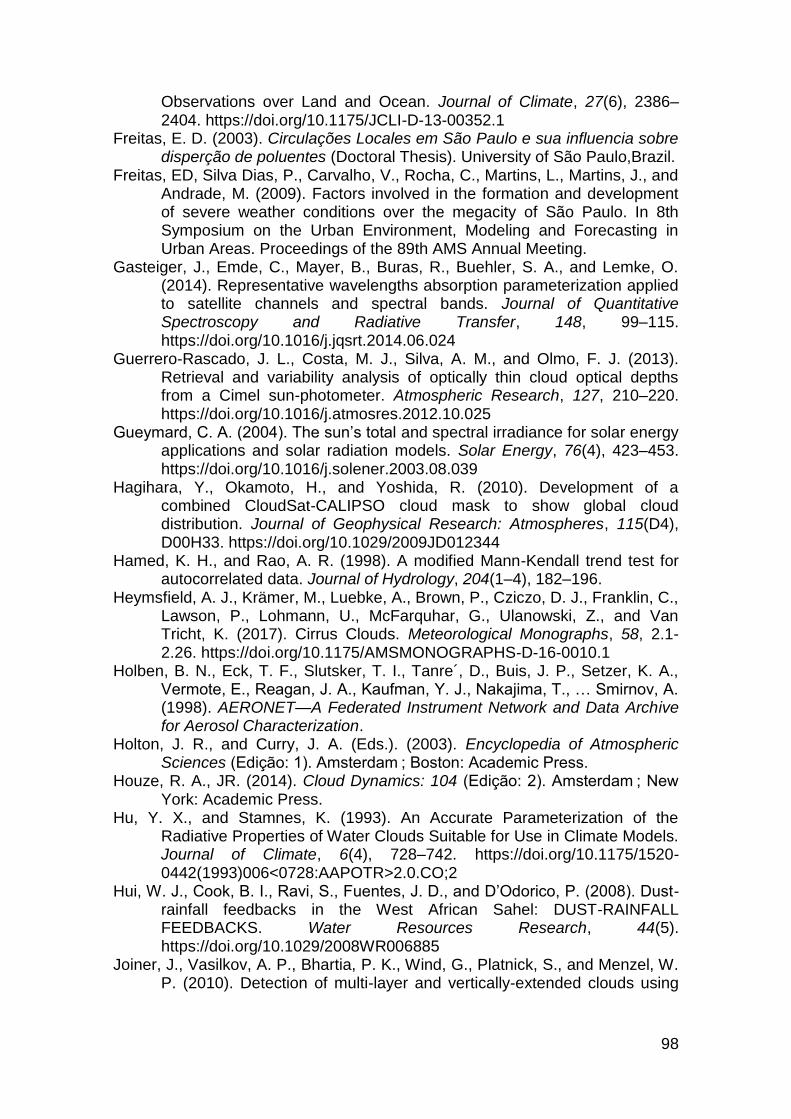
98
Observations over Land and Ocean. Journal of Climate, 27(6), 2386–2404. https://doi.org/10.1175/JCLI-D-13-00352.1
Freitas, E. D. (2003). Circulações Locales em São Paulo e sua influencia sobre disperção de poluentes (Doctoral Thesis). University of São Paulo,Brazil.
Freitas, ED, Silva Dias, P., Carvalho, V., Rocha, C., Martins, L., Martins, J., and Andrade, M. (2009). Factors involved in the formation and development of severe weather conditions over the megacity of São Paulo. In 8th Symposium on the Urban Environment, Modeling and Forecasting in Urban Areas. Proceedings of the 89th AMS Annual Meeting.
Gasteiger, J., Emde, C., Mayer, B., Buras, R., Buehler, S. A., and Lemke, O. (2014). Representative wavelengths absorption parameterization applied to satellite channels and spectral bands. Journal of Quantitative Spectroscopy and Radiative Transfer, 148, 99–115. https://doi.org/10.1016/j.jqsrt.2014.06.024
Guerrero-Rascado, J. L., Costa, M. J., Silva, A. M., and Olmo, F. J. (2013). Retrieval and variability analysis of optically thin cloud optical depths from a Cimel sun-photometer. Atmospheric Research, 127, 210–220. https://doi.org/10.1016/j.atmosres.2012.10.025
Gueymard, C. A. (2004). The sun’s total and spectral irradiance for solar energy applications and solar radiation models. Solar Energy, 76(4), 423–453. https://doi.org/10.1016/j.solener.2003.08.039
Hagihara, Y., Okamoto, H., and Yoshida, R. (2010). Development of a combined CloudSat-CALIPSO cloud mask to show global cloud distribution. Journal of Geophysical Research: Atmospheres, 115(D4), D00H33. https://doi.org/10.1029/2009JD012344
Hamed, K. H., and Rao, A. R. (1998). A modified Mann-Kendall trend test for autocorrelated data. Journal of Hydrology, 204(1–4), 182–196.
Heymsfield, A. J., Krämer, M., Luebke, A., Brown, P., Cziczo, D. J., Franklin, C., Lawson, P., Lohmann, U., McFarquhar, G., Ulanowski, Z., and Van Tricht, K. (2017). Cirrus Clouds. Meteorological Monographs, 58, 2.1-2.26. https://doi.org/10.1175/AMSMONOGRAPHS-D-16-0010.1
Holben, B. N., Eck, T. F., Slutsker, T. I., Tanre´, D., Buis, J. P., Setzer, K. A., Vermote, E., Reagan, J. A., Kaufman, Y. J., Nakajima, T., … Smirnov, A. (1998). AERONET—A Federated Instrument Network and Data Archive for Aerosol Characterization.
Holton, J. R., and Curry, J. A. (Eds.). (2003). Encyclopedia of Atmospheric Sciences (Edição: 1). Amsterdam ; Boston: Academic Press.
Houze, R. A., JR. (2014). Cloud Dynamics: 104 (Edição: 2). Amsterdam ; New York: Academic Press.
Hu, Y. X., and Stamnes, K. (1993). An Accurate Parameterization of the Radiative Properties of Water Clouds Suitable for Use in Climate Models. Journal of Climate, 6(4), 728–742. https://doi.org/10.1175/1520-0442(1993)006<0728:AAPOTR>2.0.CO;2
Hui, W. J., Cook, B. I., Ravi, S., Fuentes, J. D., and D’Odorico, P. (2008). Dust-rainfall feedbacks in the West African Sahel: DUST-RAINFALL FEEDBACKS. Water Resources Research, 44(5). https://doi.org/10.1029/2008WR006885
Joiner, J., Vasilkov, A. P., Bhartia, P. K., Wind, G., Platnick, S., and Menzel, W. P. (2010). Detection of multi-layer and vertically-extended clouds using

99
A-train sensors. Retrieved from http://ntrs.nasa.gov/search.jsp?R=20110014293
Key, J. R., Yang, P., Baum, B. A., and Nasiri, S. L. (2002). Parameterization of shortwave ice cloud optical properties for various particle habits. Journal of Geophysical Research: Atmospheres, 107(D13), AAC 7-1. https://doi.org/10.1029/2001JD000742
Kruskal, W. H., and Wallis, W. A. (1952). Use of Ranks in One-Criterion Variance Analysis. Journal of the American Statistical Association, 47(260), 583–621. https://doi.org/10.2307/2280779
Kurucz, R. L. (1994). Synthetic Infrared Spectra (pp. 523–531). Dordrecht: Springer Netherlands.
Landulfo, E., Larroza, E. G., Lopes, F. J. S., and Hoareau, C. (2009). A preliminary classification of cirrus clouds over Sao Paulo city by systematic lidar observations and comparison with CALIPSO and AERONET data. In R. H. Picard, K. Schäfer, A. Comeron, and M. van Weele (Eds.) (p. 747506). https://doi.org/10.1117/12.829923
LeBlanc, S. E., Pilewskie, P., Schmidt, K. S., and Coddington, O. (2015). A spectral method for discriminating thermodynamic phase and retrieving cloud optical thickness and effective radius using transmitted solar radiance spectra. Atmospheric Measurement Techniques, 8(3), 1361–1383. https://doi.org/10.5194/amt-8-1361-2015
Lee, H. (2016). Analysis of Carbon Dioxide and Cloud Effects on Temperature in Northeast China. Procedia Computer Science, 91, 690–699. https://doi.org/10.1016/j.procs.2016.07.172
Leontyeva, E., and Stamnes, K. (1994). Estimations of Cloud Optical Thickness from Ground-Based Measurements of Incoming Solar Radiation in the Arctic. Journal of Climate - J CLIMATE, 7(4), 566–578. https://doi.org/10.1175/1520-0442(1994)007<0566:EOCOTF>2.0.CO;2
Liou, K. N. (2002). An Introduction to Atmospheric Radiation (Edición: 2). Amsterdam ; Boston: Academic Press.
Mace, G. (2007). Level 2 GEOPROF product process description and interface control document algorithm version 5.3. NASA Jet Propulsion Laboratory.
Mahoney, W. P. (1988). Gust Front Characteristics and the Kinematics Associated with Interacting Thunderstorm Outflows. Monthly Weather Review, 116(7), 1474–1492. https://doi.org/10.1175/1520-0493(1988)116<1474:GFCATK>2.0.CO;2
Manton, M. J. (1980). Computations of the effect of cloud properties on solar radiation. Journal de Recherches Atmosphériques, 14, 1–16.
Marchand, R., Mace, G. G., Ackerman, T., and Stephens, G. (2008). Hydrometeor Detection Using Cloudsat—An Earth-Orbiting 94-GHz Cloud Radar. Journal of Atmospheric and Oceanic Technology, 25(4), 519–533. https://doi.org/10.1175/2007JTECHA1006.1
Marín, M. J., Serrano, D., Utrillas, M. P., Núñez, M., and Martínez-Lozano, J. A. (2017). Effective cloud optical depth and enhancement effects for broken liquid water clouds in Valencia (Spain). Atmospheric Research, 195, 1–8. https://doi.org/10.1016/j.atmosres.2017.05.008
Marshak, A., Knyazikhin, Y., Davis, A. B., Wiscombe, W. J., and Pilewskie, P. (2000). Cloud-vegetation interaction: Use of normalized difference cloud
100
index for estimation of cloud optical thickness. Geophysical Research Letters, 27(12), 1695–1698.
Marshak, A., Knyazikhin, Y., Evans, K. D., and Wiscombe, W. J. (2004). The “RED versus NIR” plane to retrieve broken-cloud optical depth from ground-based measurements. Journal of the Atmospheric Sciences, 61(15), 1911–1925.
Mateos, D., Antón, M., Valenzuela, A., Cazorla, A., Olmo, F. J., and Alados-Arboledas, L. (2013). Short-wave radiative forcing at the surface for cloudy systems at a midlatitude site. Tellus B: Chemical and Physical Meteorology, 65(1), 21069. https://doi.org/10.3402/tellusb.v65i0.21069
Mateos, D., Antón, M., Valenzuela, A., Cazorla, A., Olmo, F. J., and Alados-Arboledas, L. (2014). Efficiency of clouds on shortwave radiation using experimental data. Applied Energy, 113, 1216–1219. https://doi.org/10.1016/j.apenergy.2013.08.060
Mayer, B., Kylling, A., Emde, C., Hamann, U., and Buras, R. (2015). libRadtran user’s guide. Edition for LibRadtran Version, 1.
McBride, P. J., Schmidt, K. S., Pilewskie, P., Kittelman, A. S., and Wolfe, D. E. (2011). A spectral method for retrieving cloud optical thickness and effective radius from surface-based transmittance measurements. Atmospheric Chemistry and Physics, 11(14), 7235–7252. https://doi.org/10.5194/acp-11-7235-2011
McPeters, R. D., Bhartia, P. K., Krueger, A. J., Herman, J. R., Wellemeyer, C. G., Seftor, C. J., Jaross, G., Torres, O., Moy, L., and Labow, G. (1998). Earth probe total ozone mapping spectrometer (TOMS): data products user’s guide.
Min, Q. (2004). Retrievals of thin cloud optical depth from a multifilter rotating shadowband radiometer. Journal of Geophysical Research, 109(D2). https://doi.org/10.1029/2003JD003964
Min, Q., and Harrison, L. C. (1996). Cloud properties derived from surface MFRSR measurements and comparison with GOES results at the ARM SGP Site. Geophysical Research Letters, 23(13), 1641–1644. https://doi.org/10.1029/96GL01488
Min, Q., Wang, T., Long, C. N., and Duan, M. (2008). Estimating fractional sky cover from spectral measurements. Journal of Geophysical Research: Atmospheres, 113(D20). https://doi.org/10.1029/2008JD010278
Morais, M. A., Castro, W. A. C., and Tundisi, josé G. (2010). Climatologia de frentes frias sobre a Região Metropolitana de São Paulo (RMSP), e sua influência na climatologia dos reservatórios de abastecimento de água. Revista Brasileira de Meteorologia, 25(2), 205–217.
Moura, L. M. de, Martins, F. R., and Assireu, A. T. (2016). Clouds cover variability in São Paulo. Revista Ambiente & Água, 11(4), 903–914.
Neiburger, M. (1949). Reflection, absorption, and transmission of insolation by stratus cloud. Journal of Meteorology, 6(2), 98–104. https://doi.org/10.1175/1520-0469(1949)006<0098:RAATOI>2.0.CO;2
Norris, J. R., Allen, R. J., Evan, A. T., Zelinka, M. D., O’Dell, C. W., and Klein, S. A. (2016). Evidence for climate change in the satellite cloud record. Nature, 536(7614), 72–75. https://doi.org/10.1038/nature18273
Obregón, G., Marengo, J., and Nobre, C. (2014). Rainfall and climate variability: long-term trends in the Metropolitan Area of São Paulo in the 20th

101
century. Climate Research, 61(2), 93–107. https://doi.org/10.3354/cr01241
Okamoto, H., Sato, K., and Hagihara, Y. (2010). Global analysis of ice microphysics from CloudSat and CALIPSO: Incorporation of specular reflection in lidar signals. Journal of Geophysical Research, 115(D22). https://doi.org/10.1029/2009JD013383
Paltridge, G. W. (1974). Infrared emissivity, short‐wave albedo, and the microphysics of stratiform water clouds. Journal of Geophysical Research, 79(27), 4053–4058. https://doi.org/10.1029/JC079i027p04053
Perlwitz, J., and Miller, R. L. (2010). Cloud cover increase with increasing aerosol absorptivity: A counterexample to the conventional semidirect aerosol effect. Journal of Geophysical Research: Atmospheres, 115(D8). https://doi.org/10.1029/2009JD012637
Pincus, R., and Baker, M. B. (1994). Effect of precipitation on the albedo susceptibility of clouds in the marine boundary layer. Nature, 372(6503), 250–252. https://doi.org/10.1038/372250a0
Rawlins, F., and Foot, J. S. (1989). Remotely Sensed Measurements of Stratocumulus Properties during FIRE Using the C130 Aircraft Multi-channel Radiometer. Journal of the Atmospheric Sciences, 47(21), 2488–2504. https://doi.org/10.1175/1520-0469(1990)047<2488:RSMOSP>2.0.CO;2
Salgueiro, V., Costa, M. J., Silva, A. M., and Bortoli, D. (2016). Effects of clouds on the surface shortwave radiation at a rural inland mid-latitude site. Atmospheric Research, 178–179, 95–101. https://doi.org/10.1016/j.atmosres.2016.03.020
Sayão, A. C. (2008). Estudo da variabilidade zonal da profundidade optica do aerossol em São Paulo a partir de radiômetros MFRSR (Dissertação de Mestrado). Universidade de São Paulo, São Paulo.
Serrano, D., Núñez, M., Utrillas, M. P., Marín, M. J., Marcos, C., and Martínez-Lozano, J. A. (2014). Effective cloud optical depth for overcast conditions determined with a UV radiometers: CLOUD OPTICAL DEPTH IN THE ERYTHEMAL BAND. International Journal of Climatology, 34(15), 3939–3952. https://doi.org/10.1002/joc.3953
Silva Dias, M. A. F., Dias, J., Carvalho, L. M. V., Freitas, E. D., and Silva Dias, P. L. (2013). Changes in extreme daily rainfall for São Paulo, Brazil. Climatic Change, 116(3–4), 705–722. https://doi.org/10.1007/s10584-012-0504-7
Sinyuk, A., Dubovik, O., Holben, B., Eck, T. F., Breon, F.-M., Martonchik, J., Kahn, R., Diner, D. J., Vermote, E. F., Roger, J.-C., … Slutsker, I. (2007). Simultaneous retrieval of aerosol and surface properties from a combination of AERONET and satellite data. Remote Sensing of Environment, 107(1–2), 90–108. https://doi.org/10.1016/j.rse.2006.07.022
Stamnes, K., Tsay, S.-C., Wiscombe, W., and Jayaweera, K. (1988). Numerically stable algorithm for discrete-ordinate-method radiative transfer in multiple scattering and emitting layered media. Applied Optics, 27(12), 2502–2509. https://doi.org/10.1364/AO.27.002502
Stephens, G. L. (2005). Cloud feedbacks in the climate system: A critical review. Journal of Climate, 18(2), 237–273.

102
Stith, J. L., Dye, J. E., Bansemer, A., Heymsfield, A. J., Grainger, C. A., Petersen, W. A., and Cifelli, R. (2002). Microphysical observations of tropical clouds. Journal of Applied Meteorology, 41(2), 97–117.
Tian, L., and Curry, J. A. (1989). Cloud overlap statistics. Journal of Geophysical Research: Atmospheres, 94(D7), 9925–9935. https://doi.org/10.1029/JD094iD07p09925
Twomey, S. (1977). The Influence of Pollution on the Shortwave Albedo of Clouds. Journal of the Atmospheric Sciences, 34(7), 1149–1152. https://doi.org/10.1175/1520-0469(1977)034<1149:TIOPOT>2.0.CO;2
Tzoumanikas, P., Nikitidou, E., Bais, A. F., and Kazantzidis, A. (2016). The effect of clouds on surface solar irradiance, based on data from an all-sky imaging system. Renewable Energy, 95, 314–322. https://doi.org/10.1016/j.renene.2016.04.026
Vernier, J.-P., Thomason, L. W., Pommereau, J.-P., Bourassa, A., Pelon, J., Garnier, A., Hauchecorne, A., Blanot, L., Trepte, C., Degenstein, D., and Vargas, F. (2011). Major influence of tropical volcanic eruptions on the stratospheric aerosol layer during the last decade. Geophysical Research Letters, 38(12), L12807. https://doi.org/10.1029/2011GL047563
Warren, S. G., Eastman, R. M., and Hahn, C. J. (2007). A Survey of Changes in Cloud Cover and Cloud Types over Land from Surface Observations, 1971–96. Journal of Climate, 20(4), 717–738. https://doi.org/10.1175/JCLI4031.1
Warren, S. G., Hahn, C. J., and London, J. (1985). Simultaneous Occurrence of Different Cloud Types. Journal of Climate and Applied Meteorology, 24(7), 658–667. https://doi.org/10.1175/1520-0450(1985)024<0658:SOODCT>2.0.CO;2
Winker, D. M., Vaughan, M. A., Omar, A., Hu, Y., Powell, K. A., Liu, Z., Hunt, W. H., and Young, S. A. (2009). Overview of the CALIPSO Mission and CALIOP Data Processing Algorithms. Journal of Atmospheric and Oceanic Technology, 26(11), 2310–2323. https://doi.org/10.1175/2009JTECHA1281.1
Wood, R. (2012). Stratocumulus Clouds. Monthly Weather Review, 140(8), 2373–2423. https://doi.org/10.1175/MWR-D-11-00121.1
Yamasoe, M. A., and Corrêa, M. de P. (2016). Processos Radiativos na Atmosfera. Fundamentos (Edição: 1). Oficina de Textos.
Yamasoe, M. A., do Rosário, N. M. E., and Barros, K. M. (2017). Downward solar global irradiance at the surface in São Paulo city-The climatological effects of aerosol and clouds: SW Aerosol and Cloud Radiative Effect. Journal of Geophysical Research: Atmospheres. https://doi.org/10.1002/2016JD025585
Yang, P., Liou K. N., Wyser Klaus, and Mitchell David. (2000). Parameterization of the scattering and absorption properties of individual ice crystals. Journal of Geophysical Research: Atmospheres, 105(D4), 4699–4718. https://doi.org/10.1029/1999JD900755
Yau, M. K., and Rogers, R. R. (1989). Short Course in Cloud Physics (Edición: 3). Oxford: Butterworth-Heinemann.
Yoshida, R., Okamoto, H., Hagihara, Y., and Ishimoto, H. (2010). Global analysis of cloud phase and ice crystal orientation from Cloud-Aerosol Lidar and Infrared Pathfinder Satellite Observation (CALIPSO) data using

103
attenuated backscattering and depolarization ratio. Journal of Geophysical Research, 115. https://doi.org/10.1029/2009JD012334