CLOUD COMPUTING SIMULATION

CLOUD COMPUTING SIMULATION

A Thesis Submitted

in partial fulfillment of the requirements

for the degree of

Master of Technology

by

Krishnadhan Das

Roll No: 09305071

under the guidance of

Prof. Purushottam Kulkarni and Prof. Umesh Bellur

Department of Computer Science and Engineering

Indian Institute of Technology, Bombay

Mumbai

Dissertation Approval Certificate

Department of Computer Science and Engineering

Indian Institute of Technology, Bombay

The dissertation entitled CLOUD COMPUTING SIMULATION, submitted by KrishndhanDas (Roll No: 0305071) is approved for the degree of Master of Technology in ComputerScience and Engineering from Indian Institute of Technology, Bombay.

Prof. Purushottam KulkarniDept CSE, IIT BombaySupervisor

Prof. Umesh BellurDept CSE, IIT Bombay

Supervisor

abcDept CSE, IIT BombayInternal Examiner

xyzx

External Examiner

xyzy

Chairperson

Place: IIT Bombay, MumbaiDate: 21st June, 2010

Abstract

Cloud computing provides opportunity to dynamically scale the computing resources for appli-cations. These resources are shared among customers using virtualization technology. Usingthese resources efficiently, is an open challenge. Since cloud computing environment has largesetup and cost associated with it, testing applications and resource allocation policies are highlychallenging. We have developed a simulator that is extension of the open source simulatorCloudSim. Cloudsim aims to help developers to model and test, applications and policies incloud computing environment. Developed as multi-layered architecture, this simulator helps totest new approaches, find the bottlenecks before implementing in real world cloud computingenvironment.

In this report, we have discussed the design and verification of features a) communicationamong entities in cloud computing entities, b) Xen virtualization overhead prediction and c)abstraction of applications, using experimental evaluation in virtualized environment. The re-sult shows that error in predicting the virtualization overhead remain within range of ± 2%.And applications can be abstracted as number of instructions or cycles needed to complete theexecution.

iii

Contents

1 Introduction 11.1 Motivation . . . . . . . . . . . . . . . . . . . . . . . . . . . . . . . . . . . . . 2

1.2 Outline of Work . . . . . . . . . . . . . . . . . . . . . . . . . . . . . . . . . . 3

2 Background 52.1 Virtualization technology . . . . . . . . . . . . . . . . . . . . . . . . . . . . . 5

2.2 Xen: Virtual machine monitor . . . . . . . . . . . . . . . . . . . . . . . . . . 7

2.3 Existing work . . . . . . . . . . . . . . . . . . . . . . . . . . . . . . . . . . . 9

3 Problem definition 113.1 List of features . . . . . . . . . . . . . . . . . . . . . . . . . . . . . . . . . . 11

3.1.1 Physical machine instance . . . . . . . . . . . . . . . . . . . . . . . . 11

3.1.2 Virtual machine instance . . . . . . . . . . . . . . . . . . . . . . . . . 11

3.1.3 Different Virtualization technology . . . . . . . . . . . . . . . . . . . 12

3.1.4 Application instance . . . . . . . . . . . . . . . . . . . . . . . . . . . 12

3.1.5 Resource allocation . . . . . . . . . . . . . . . . . . . . . . . . . . . . 13

3.1.6 Placement Policies . . . . . . . . . . . . . . . . . . . . . . . . . . . . 13

3.1.7 Migration policies . . . . . . . . . . . . . . . . . . . . . . . . . . . . 13

3.1.8 Network topology and communication among entities . . . . . . . . . 14

3.1.9 Price model . . . . . . . . . . . . . . . . . . . . . . . . . . . . . . . . 14

3.2 Our contribution . . . . . . . . . . . . . . . . . . . . . . . . . . . . . . . . . . 14

4 Cloudsim simulator Internals 154.1 Architecture of Cloudsim . . . . . . . . . . . . . . . . . . . . . . . . . . . . . 15

4.1.1 Modelling the cloud computing environment . . . . . . . . . . . . . . 15

4.1.2 Modelling the cloud Application and workload . . . . . . . . . . . . . 16

4.1.3 Modelling the datacenter . . . . . . . . . . . . . . . . . . . . . . . . . 17

4.1.4 Modelling of Physical and virtual machine . . . . . . . . . . . . . . . 17

4.1.5 Modelling of communication . . . . . . . . . . . . . . . . . . . . . . . 17

4.1.6 Modelling power consumption . . . . . . . . . . . . . . . . . . . . . . 18

4.1.7 Manager module . . . . . . . . . . . . . . . . . . . . . . . . . . . . . 19

v

4.2 Design of Cloudsim . . . . . . . . . . . . . . . . . . . . . . . . . . . . . . . . 194.3 Extension of Cloudsim . . . . . . . . . . . . . . . . . . . . . . . . . . . . . . 21

5 Virtualization overhead and communication among applications in cloudsim 235.1 Design of communication among entities in cloudsim . . . . . . . . . . . . . . 235.2 Virtualization overhead model . . . . . . . . . . . . . . . . . . . . . . . . . . 26

6 Verification of virtualization overhead prediction and application abstraction 316.1 Virtualization overhead . . . . . . . . . . . . . . . . . . . . . . . . . . . . . . 316.2 Application (cloudlet) characteristics verification . . . . . . . . . . . . . . . . 35

7 Correctness and capabilities of cloudsim 397.1 Test cases of communication among applications . . . . . . . . . . . . . . . . 39

7.1.1 Communication among two applications running on different physicalmachine . . . . . . . . . . . . . . . . . . . . . . . . . . . . . . . . . . 39

7.1.2 Multiple communications among applications running on different phys-ical machine . . . . . . . . . . . . . . . . . . . . . . . . . . . . . . . 41

7.1.3 Communication among applications with soft resource allocation pol-icy at physical host level . . . . . . . . . . . . . . . . . . . . . . . . . 43

7.2 Experiment using cloudsim . . . . . . . . . . . . . . . . . . . . . . . . . . . . 45

8 Summary and Conclusions 49

9 Appendix 519.1 Configuration and input files of cloudsim . . . . . . . . . . . . . . . . . . . . 51

9.1.1 System configuration . . . . . . . . . . . . . . . . . . . . . . . . . . . 519.1.2 Input specification . . . . . . . . . . . . . . . . . . . . . . . . . . . . 53

List of Figures

2.1 Structure of xen hypervisor [6] . . . . . . . . . . . . . . . . . . . . . . . . . . 72.2 Network i/o activity in xen hypervisor [6] . . . . . . . . . . . . . . . . . . . . 9

4.1 Block diagram of CloudSim [4] . . . . . . . . . . . . . . . . . . . . . . . . . 164.2 Cloudsim class diagram [4] . . . . . . . . . . . . . . . . . . . . . . . . . . . . 194.3 Cloudsim sequence diagram [4] . . . . . . . . . . . . . . . . . . . . . . . . . 20

5.1 Cloudsim UML class diagram after implementation . . . . . . . . . . . . . . . 245.2 Cloudsim sequence diagram . . . . . . . . . . . . . . . . . . . . . . . . . . . 255.3 Cloudsim sequence diagram of distribution of bandwidth among applications . 265.4 Domain-0 and domain-u cpu utilization vs disk read at guest domain . . . . . . 275.5 Domain-0 and domain-u cpu utilization vs network data rate at guset domain . 28

6.1 Experiment setup [8] . . . . . . . . . . . . . . . . . . . . . . . . . . . . . . . 326.2 Comparison of predicted and actual domain-0 cpu utilization at physical ma-

chine 1 . . . . . . . . . . . . . . . . . . . . . . . . . . . . . . . . . . . . . . . 336.3 Comparison of predicted and actual domain-0 cpu utilization at physical ma-

chine 2 . . . . . . . . . . . . . . . . . . . . . . . . . . . . . . . . . . . . . . . 346.4 Prediction error of domain-0 cpu utilization on different physcal machines . . . 34

7.1 Setup of test case 1 . . . . . . . . . . . . . . . . . . . . . . . . . . . . . . . . 407.2 Setup of test case 2 . . . . . . . . . . . . . . . . . . . . . . . . . . . . . . . . 427.3 Setup of test case 3 . . . . . . . . . . . . . . . . . . . . . . . . . . . . . . . . 447.4 Resource requirement and availability in soft vs hard allocation policy in virtual

machines . . . . . . . . . . . . . . . . . . . . . . . . . . . . . . . . . . . . . 467.5 Total resource utilization in soft vs hard allocation in physical machines . . . . 47

vii

List of Tables

4.1 BRITE format: node representation [10] . . . . . . . . . . . . . . . . . . . . . 184.2 BRITE format: link representation [10] . . . . . . . . . . . . . . . . . . . . . 184.3 Implementation status of the features specified in section 3.1 . . . . . . . . . . 22

6.1 Tabulation of the matrics used for modelling . . . . . . . . . . . . . . . . . . . 326.2 Experimental evaluation of application abstraction . . . . . . . . . . . . . . . . 36

7.1 Test case: communication among two applications running on different physicalmachine . . . . . . . . . . . . . . . . . . . . . . . . . . . . . . . . . . . . . . 41

7.2 Test case: a pair of communication among applications running on differentphysical machine . . . . . . . . . . . . . . . . . . . . . . . . . . . . . . . . . 43

7.3 Test case: a pair of communication among applications running on differentphysical machine, with allocation policy soft at the physical machine level . . . 45

ix

Chapter 1

Introduction

Cloud computing is an approach of using computing as utility. Relatively new term for repre-senting collection of resources which are shared, scaled dynamically. Based on ”pay as you use”model, resources can be used or released whenever needed. This refers to both, applications asservice to users and servers in datacenters which support those services. Cloud computing is aparadigm of distributed computing to provide the customers on-demand, utility based comput-ing services. Cloud itself consists of physical machines in the data centers of cloud providers.Virtualization technology is used on this physical machines to run multiple operating systemssimultaneously.

We can define cloud computing as collection of resources (servers in datacenter), which areinterconnected with each other and using virtualization technology can be scaled and adapteddynamically. Cloud computing provides customers, to start their business without purchasingany physical hardware, whereas service providers can rent their resources to customers andmake their profit. Customers has the opportunity to scale up or down, the resources dynami-cally to provide QoS for demand varying application. Cloud computing enables dynamic andflexible application provisioning using virtualization technology.

Beneficiaries of cloud computing can be divided into a) cloud computing providers, b) cloudcomputing customers and c) end-users [1]. Cloud service providers owns the physical resourcesas datacenters. Cloud computing customers, use this resources to provide service to customers.And end-users use those services. For example any particular online newspaper uses Ama-zon EC2 for hosting their web site. Here Amazon EC2 is the cloud computing provider andnewspaper publisher is the cloud customer. And newspaper readers are the end-users. Duringthe morning period, number of end-users increases and load on hosting servers increases. Asa result response time of website increases. Here cloud computing providers can increase thenumber of hosting servers and bandwidth of this website to maintain a certain response timelimit. And when the end-users reduces over-allocated servers can be released.

1

In practical cases cloud computing service providers maintain a collection of large data cen-ters throughout the globe to satisfy customer requirement. To use the resources efficiently andproviding service to the customers, application placement and resource allocation policies areimplemented. These application placement policies can produce different levels of profit/lossfor the service provider. Measuring the performance of policies directly on real environmentor emulating is time-consuming and difficult. Some of the reasons are a) cloud computing in-frastructure consists of large number of physical machines, b) service provider may not providesufficient low low level access to physical machines and c) applications in cloud computinghave varying demand, configuration and resource utilization.

1.1 Motivation

Since cloud computing essentially has commercial purpose, there are different policies followedby the service providers. These policies can be a) application placement policy, b) resourcesharing among multiple clients and c) pricing models. Application policies can aim at serverconsolidation or load-balancing. In server consolidation, aim is to minimize the active numberof servers. While load balancing aims to fairly distribute the load among all active servers.Resource sharing can provide flexibility or rigidity in case of an unexpected load burst. Usingdynamic scaling, number of active servers can be increased instantly to server unexpected loadbursts. While price model can be, pay as you used or on based on fixed model. Researchers havedeveloped numerous resource allocation policies like topology-aware, communication aware,prediction based, temperature or energy aware. This policies can be applied at the initial timeor dynamically. There have been also research on the architecture of datacenter, focusing ofnetwork infrastructure and component failure. All this policies are intended to be used in data-centers, consisting of thousands of servers and thus scalability is an important factor. Normallyresearchers tend to use small number of server and assumes many parameters in their experi-mental evaluation. Which may not perform as expected in case of large scale setup.

Now for example, we want to develop a resource allocation policy which predicts the im-mediate future behaviour and dynamically scales up or down, number of active servers. Aimis to provide an acceptable service time while maintaining a sufficiently high utilization of theactive servers. This policy has to predict future behaviour and threshold load, after which activenumber of servers should be increased or decreased. To deploy this policy, we need to test thisnew resource allocation policy on large number of servers which can a) produce unpredictableresult and affect the existing system, b) needs major modification of existing system. And sincethis testing has to be done at large scale, whole datacenter may needs to down for testing. Other

2

problems can be re-designing of the whole testing set-up over multiple runs. All this issues withscalability and huge cost associated with datacenter makes testing any new policy an impracti-cal task.

Another approach is to use simulator. Simulator can help to a) easily create large set-up forthe experiment , b) produce controlled experiment environment and c) experiment with differ-ent varying parameters. Considering the challenges of testing and implementation of new ideasin cloud computing, we have listed the possible requirements of an ideal cloud computing sim-ulator. There have been research on grid computing simulator like GridSim [13], SimGrid [12]but none of them fulfills the requirements of cloud computing simulator. Evaluating existingavailable open source simulator CloudSim [4] and potential scope for extension, we have decideto build new features in this simulator instead of build new simulator from scratch.

1.2 Outline of Work

In this report we describe the necessary addition, changes and verification process to add twomain feature a) communication among entities (cloud computing applications) b) virtualizationoverhead prediction, in cloudsim. Remaining of part of the report is structured as follows. Chap-ter 2 describes background of virtualization, Xen hypervisor and existing simulator. Chapter 3describes the list of features of an ideal cloud computing simulator and features we have de-veloped. Chapter 4 describes the design, implementation and possible extensions of cloudsim,on which we have developed some features. Chapter 5 discusses the necessary additions andmodification of cloudsim to extend with the newly developed features. Chapter 6 discusses theexperiment conducted to verify the developed features. Chapter 7 describes the different testcases for checking correctness and simple experiment to show capability of cloudsim. Chapter8 describes the overall summary of our work, future work and concludes.

3

4

Chapter 2

Background

This section presents the background on different components of cloud computing.

2.1 Virtualization technology

Virtualization technology enables to run multiple operating systems (or virtual machines) si-multaneously on a single physical machine sharing the same underlying resources. Some ofthe reason for using virtualization is a) sufficient capability of recent computers to run multi-ple operating systems, b) using multiple isolated operating systems, resource utilization can bemaximized, c) ability to run different operating systems on single physical machine (for exam-ple Linux and Windows).

The software layer which provides the virtualization of underlying hardware is called hy-pervisor. Hypervisor emulates the underlying hardware resources to the different operatingsystems (virtual machine). Normally operating system has the direct access to the underlyinghardware of a physical machine. In case of virtualization, operating systems access the hard-ware through the hypervisor. Hypervisor executes the privileged instruction on behalf of virtualmachine. Virtualization technology enables to allocate resources of single physical machineamong multiple different users. Some of the popular virtualization technologies are XEN [2],KVM [3]. In cloud computing, virtualization technology is used to create/destroy virtual ma-chine to dynamically allocate/reduce resources for an application. Also virtualization helps toco-locate virtual machines to a small number of physical machines, such that number of activephysical machines can be reduced. This approach is called server consolidation.

Virualization can mainly be divided into three different types a) full virtualization, b) paravirtualization and c) Hardware-assisted virtualization. Full virtualization emulates completeunderlying hardware to the virtual machines, thus allowing unmodified guest operating systemto run. Para virtualization provides an idealized underlying hardware interface to the guest sys-

5

tems, so guest operating system needs modification. In case of hardware assisted virtualizationthe hardware provides special instructions that help to execute privileged instructions, here alsoguest operating system does not need any modification. To support multiple guest operatingsystems sharing same common resources, virtualization layer has to provide an interface of allthe resources. These resources are cpu, main memory i/o and devices. Virtualizing all thisresources produce different challenges. In case of cpu, there are four protection rings, namedring 0, 1, 2, 3 with descending privileged in nature. And operating system and user space ap-plications run at ring 0 and 3 respectively. Since hypervisor now runs at ring 0, in case of cpuvirtualization, challenge is to handle privileged instructions executed by guest operating sys-tems, like instructions updating page table.

Para virtualization: Provides closest possible underlying hardware interface to the guestoperating system. Guest operating systems are aware of the virtualized environment and run atring 1. Privileged instructions are replaced by hypercalls that correspond to them. This replace-ment is done at compile time, while modifying the guest kernel. Hypervisor traps this hypercallsand passes control to the guest os. For managing memory table, one extra layer of indirection isadded, mapping each guest operating systems memory page table to hardware page table whichis maintained by hypervisor. Para virtualization is also called software virtualization, becauseof these modifications are done at software level.

Hardware assisted virtualization: Provides an additional set of instructions, which createan extra ring layer ”ring -1”, thus allowing unmodified guest operating systems to run at ring-0.Privileged instructions are handled by hypervisor at ring -1 and control is passed back to guestoperating systems. This provides nested page tables which allows multi-level paging in hard-ware level. Since page translation is done at hardware level, this is almost same fast as normaloperating system memory lookup.

Virtualization supports migration of virtual machines from current to other physical ma-chines. Migration process transfers the main memory pages and states of virtual machine to atarget machine. Migration policy decides when, which and where to migrate a virtual machine.One example is, there is high load on a physical machine and not sufficient resource avail-able for a virtual machine, that virtual machine is migrated to a less utilized physical machine.Placement policy decides where to put a newly created virtual machine. For example, this maydepend on current resource utilization of physical machine or number of already running virtualmachines or type of applications that will run on virtual machine. Since in cloud computing,applications experience high variation of demand, virtualization can dynamically help to allo-cate resources.

Some of the challenges of virtualization are placement policy of virtual machine, migration

6

Figure 2.1: Structure of xen hypervisor [6]

policy of virtual machines, maintaining performance level. Researches develop new policies orapproaches to solve this challenges. Using Cloudsim simulator, currently some of these policiescan be modelled and tested on a controlled environment, with large set-up.

2.2 Xen: Virtual machine monitor

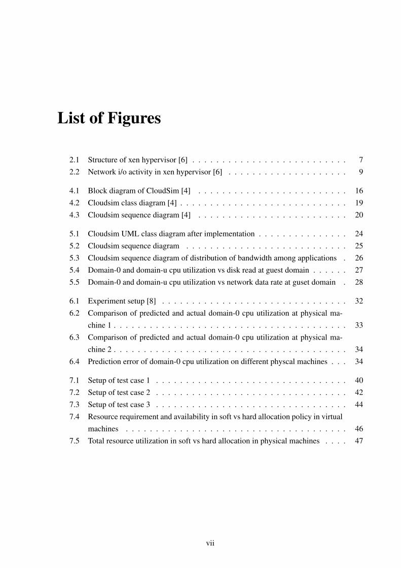
Xen is one of popular virtual machine monitor, which uses para virtualization technology. Maincomponents are hypervisor or virtual machine monitor, guest operating systems or domains andapplications. Hypervisor provides an abstraction of underlying hardware to guest operatingsystems, called domains. Since Xen uses para virtualization, most of device driver componentsof an operating system is placed in a privileged domain called domain-0. Domain-0 also pro-vides the management, it allows to create, destroy, migrate any guest domains. Since dom-0 hasall the device drivers, it handles different i/o activity like network and disk on behalf of guestdomains. Figure 2.1 shows the structure of xen hypervior.

Profiling and modelling of resource usage in Xen environment is one of major research area.Since domain-0 handles the different i/o activity on behalf of guest domains, resource utiliza-tion at domain-0 is important. Correct prediction of the domain-0 overhead due to guest domainactivity helps in decision making like capacity building, placement and migration policies. Inour work, we have developed feature in cloudsim to predict domain-0 overhead using linearregression model.

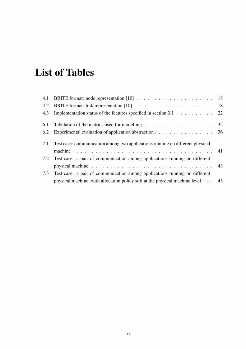
Xen networking: Figure 2.2 shows the internal mechanism of network activity of xen hy-

7

pervisor. Since Xen use para virtualization technology, all of the real device drivers are indomain-0. There is a pair of split device driver in guest domain and domain-0 called, front-end and back-end respectively. There is also abstraction of virtual firewall router in domain-0.In case of packet sent by an application, the packet reaches front-end driver and using sharedmemory to back-end driver. Here depending upon the destination address, routing decision ismade. If the destination address belongs to some other guest operating systems running onsame physical machine, packet is sent to that guest domains front-end driver. Else the packet isactually sent by actual device driver to the physical hardware. In case of packet reception fromthe physical hardware, the virtual router selects the destination domain and forward the packetto it’s front-end device driver.

So in case of communication among guest domains running on same physical machines,only permission of memory pages corresponding to network packets have to be changed. Net-work packets does not need to go to the real device driver. And the delay between transmissionand reception of packets become very low, as a result very high data rate rate is possible. Theimplications are that, resource utilization at domain-0 is very less in case of communicationamong guest domains on same physical machine than communication among guest domains re-siding on different physical machines. This provides an extra dimension for application place-ment in virtualized environment. Multi-tier applications which communicate with each othercan be placed on different guest domains on same physical machines for better performance. Sopredicting the performance behaviour of applications running in non-virtualized environment tovirtualized environment depends on type of communications among the components.

Cpu scheduling: There has been a lot of different cpu scheduler used over the developmentcycle of xen. Currently xen 4.0 uses credit scheduler for cpu scheduling. Work conservingscheduling means, the resource will be used, if there is any work left. In case of cpu scheduling,work conserving means cpu will be utilized at 100%, if there is any process or guest domain hasto work. In credit scheduling, each domain has two associated parameters a) cap and b) weight.Weight defines the relative priorities among domains, whereas cap defines the maximum limit.Summation of the all the domain’s cap should be less than total cpu capacity. If the cap isdefined, then the scheduler will behave as non-conserving scheduler. By default, credit basedscheduler works as work conserving in nature and cpu is utilized, if there is any work.

I/O scheduling: Xen uses round robin scheduling to perform i/o activty (both disk and i/o).There is currently no dynamic in-built tool to isolate i/o performance among different domains.Lot of researchers have developed tools to isolate the i/o perormance isolation in xen. If thetotal i/o activity requirement is less than maximum capacity, i/o scheduler behave as work-conserving scheduler.

8

Figure 2.2: Network i/o activity in xen hypervisor [6]

2.3 Existing work

Cloudsim [4, 5] is an existing open source cloud computing simulation developed at Universityof Melbourne. We have discussed the architecture and design of Cloudsim in details in chapter4. Currently cloudsim provides system and behaviour modelling of data centers, virtual ma-chines, physical machines and cloud computing applications. Also simple abstraction of place-ment policies for virtual machine and applications are implemented. Some of the importantfeatures like a) virtualization overhead prediction for different technologies, b) communicationamong entities, c) migration of virtual machines and it’s overhead, and d) dynamic resourcesharing and application placement are the potential extensions of Cloudsim.

In this chapter, we have discussed the different virtualization technologies and specificallyXen internals. Because we have developed feature to predict the Xen virtualization overhead inthe Cloudsim. Different components like cpu scheduling, i/o scheduling of Xen virtualizationhas been discussed here. At the end, we have briefly introduced Cloudsim simulator, on whichwe have worked.

9

10

Chapter 3

Problem definition

Our goal is to develop a simulator for academic and industrial purpose, to model and test newpolicies for better utilization of the cloud infrastructure. With assumption that, virtualizationtechnologies are used for resource sharing. Using this simulator, performance and utilization ofresources will be measured for resource allocation policies and application scheduling. Devel-opers will able to add their placement and migration policy to test, the overall performance ofthe system.

This simulator will help to model and analyze different components of cloud computing.Using this simulator, cloud service providers can measure the performance of the applicationsrunning on behalf of the customers. Here is the list of features of an ideal cloud computingsimulator.

3.1 List of features

3.1.1 Physical machine instance

Ability to simulate a physical machine instance with different hardware specification. This is thehigh-level abstraction of physical machine. Abstraction is that physical machine is collection ofresource. These resources are shared among multiple virtual machine, by using virtualizationtechnology. Interface will allow to create, start, stop and destroy virtual machines within aphysical machine. Also interface will provide different kind of options to configure and assignpriorities among different virtual machines.

3.1.2 Virtual machine instance

Ability to simulate a virtual machine instance with specific resource requirement and virtualiza-tion technology. This high-level abstraction of virtual machine. Abstraction is virtual machine

11

runs on host physical machine, uses the share of underlying resources to complete execution ofapplications. Interface will allow to submit and withdraw applications in a virtual machine.

3.1.3 Different Virtualization technology

Based on requirement and specification, any virtualization technology can be used. User shouldbe able to mention what kind of virtualization technology, will be used. Depending upon thetechnology, different features provided by that technology will be provided. Like in case ofXen, we will provide controlling domain and guest domains to the users.

One of the main important advantage of virtualization is ability to migrate virtual machines.Migration process, affects the resource usage of the source and destination machines. In boththe machines, cpu usage and bandwidth usage increases significantly. This overhead due tomigration is an important factor for decision making in case of migration and resource allocationpolicy. Also migration enables dynamic resource allocation among virtual machines.

3.1.4 Application instance

Ability to simulate applications with different configurations. Applications run on specific ma-chine (fulfilling requirements) on a specific time. Abstraction of an application is that it is acollection of resource usage, which can be dependent or independent on external issues, butdepending upon available hardware resources it can finish early/late. While representing anapplication’s characteristics, there should be a lot of choices to the user, how resource require-ment can be represented. Because applications can have different requirement, different setupor different resource intensive. For example a) specification of resource requirement to serveone unit of request and number of total request over the time period b) for specifying multi-tierapplication, input specification of one application will be output of other application.

Applications using different resources simultaneously, should have the concept of a) depen-dency among resources b) interference among resources. Also applications can be divided intodifferent types and application execution models. Some general properties of any applicationcan be defined as a) different resource utilization b) execution-time length c) size of data bytesread or write form disk d) deployment requirements.

Applications into two types. a) Standalone application. b) Multi-tier application : Collectionof standalone applications, which fulfills a larger goal. Here we will basically specify, whatis amount of communication among this standalone applications. For example, to provide aweb-based service, a collection of servers are used. These are web, application and databaseservers. Request are collected by web server, then forwarded to application server and then

12

to database server. But only some fraction of these requests are sent to next level and rest areserved from cached information. So still all servers are running standalone applications, thereis some relationship among them. These relationship could be provided to the simulator.

Execution models a) Server/client model : waits for request from clients and serve them.Ex: web-server, b) Earliest finish : Kind of batch process, uses maximum available resource, tofinish at earliest. Application characteristics : a) Hardware (resource) requirement, b) Resourceutilization snd c) Start and finish time.

3.1.5 Resource allocation

Resource allocation policies decides the amount of resource to be allocated to a particular orset of virtual machines. This policy can also update the resource allocation dynamically. Forimplementing prioritization, we can provide more resource to a particular virtual machine, thanother virtual machine. Resources can be interfering or sharing with each-other. Like diskusage generates cpu utilization. Also resource can use different technologies. For examplestorage system area can use different technologies, like direct area storage, network area storage.Different technologies have different seek latency, cpu overhead.

3.1.6 Placement Policies

Placement policies both refer to virtual machine and application placement policies. Virtualmachine placement policy decides the target physical host based on some parameter value. Andapplication placement depends on, available resource and number of applications running onvirtual machines. Placement policies can be classified as a) initial placement policy b) dynamicplacement policy. Initial placement policy is executed at the start-up time of an application orvirtual machine placing. Whereas dynamic placement policy is executed during the runtimedepending upon different parameters like availability of different resources, violation of servicelevel agreements.

3.1.7 Migration policies

Migration policies decides when, which and where to migrate a virtual machine. This policiesspecify, the limiting condition which triggers a specific virtual machine to migrate. The targetmachine, which also to be manipulated should satisfy some condition. For example, a virtualmachine should be migrated when the load produced by the running application is higher than90% of virtual machines capacity. The selected target physical machine should have sufficienthigh resource available for hosting the migrated virtual machine. This resource availabilitycondition can be twice of the previous resource allocation.

13

3.1.8 Network topology and communication among entities

In a datacenter environment, all the the physical machines are inter-connected with high speedLAN connection. Network topology represents the communication among all the physicalservers by bandwidth of the links and distance between each two points. Communication amongapplications is an essential part of simulating cloud computing applications. Distribution of thenetwork bandwidth among the entities is part of resource sharing implemented by both virtualand physical machine instance.

3.1.9 Price model

In practical cases, cloud service providers rent physical machines or run application to cus-tomers. This is based on some price model. Price model can be based on specific hardwarespecification or resource usage. Depending upon type of rent, different price model and powerusage model can be implemented. Price model helps to calculate amount of saving by usingcloud computing services.

3.2 Our contribution

In this thesis work, we have developed and verified some of the features specified in the previ-ous section in Cloudsim. These features are a) communication among applications , b) Virtu-alization overhead prediction of Xen virtualization technology and c) abstraction of applicationcharacteristics . Our results show that, virtualization overhead model built from experimentaldata can predict the domain-0 cpu utilization with error ranging with ± 2%. And applicationscan be abstracted by number of instructions or cycles needed to complete the execution.

14

Chapter 4

Cloudsim simulator Internals

Currently Buyya et al. [4, 5] are developing CloudSim, which helps to model and simulate,cloud computing infrastructures and application services. Cloudsim is discrete event basedsimulator. Every event represents an change in overall system status. Whenever an event occurs,event driven simulation engine processes the events and updates the system status. CurrentlyCloudsim supports basic modelling and simulation of cloud computing infrastructure, servicebrokers, application scheduling, allocations policies, network behaviour, federation of clouds,different workload generation, power consumption and dynamic entity creation.

4.1 Architecture of Cloudsim

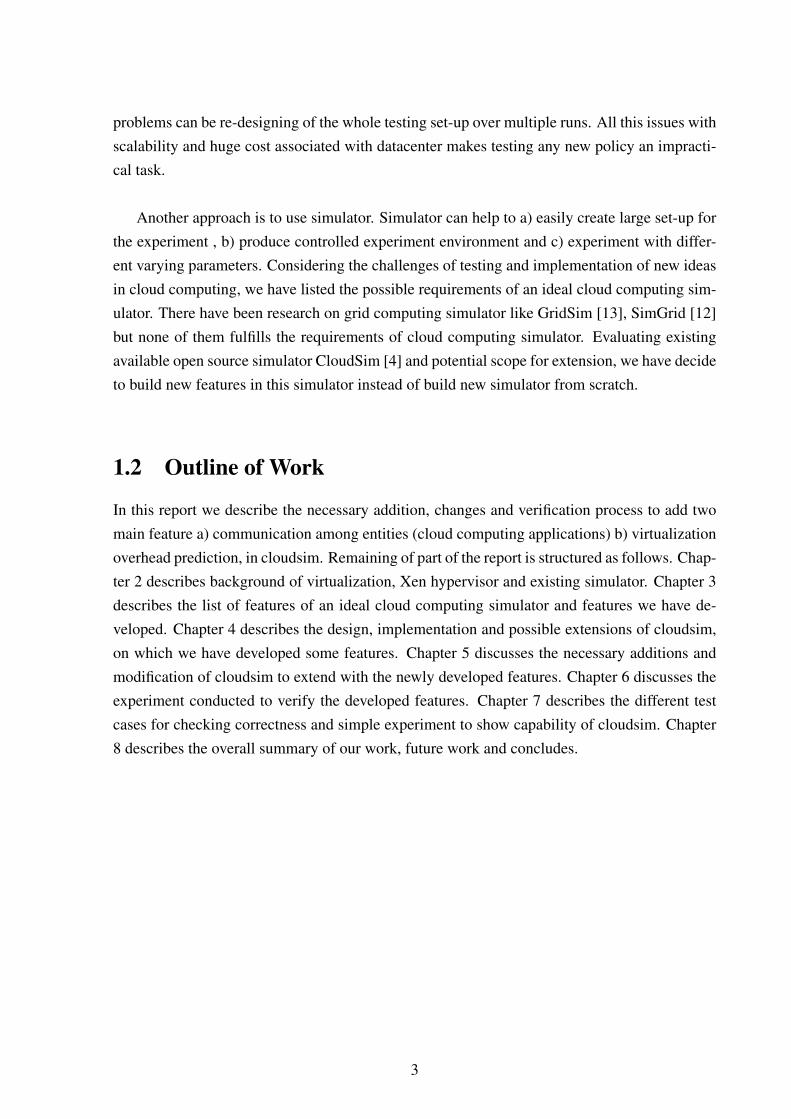
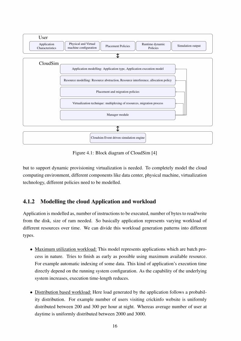
Figure 4.1 shows the basic block diagrams of cloudsim architecture. Main components area) user level specification b) cloudsim components c) event driven simulation engine. Usergiven details about the specifications of physical, virtual machines and application characteris-tics. Cloudsim components provide the abstraction different components of cloud computingenvironment like, virtual, physical machine, static placement policies. Event driven simulationengine processes the events and update the system states.

4.1.1 Modelling the cloud computing environment

As stated earlier, we can define cloud computing as collection of resources which are inter-connected and can scaled down or up dynamically. So in simulation, we can abstract cloudcomputing as collection of resources which are represented by datacenters consisting of largenumber of physical machine. This physical machines can use any virtualization technique tosupport multiple virtual machines. Number of running virtual machines and their placement canbe changed dynamically over time. Applications are submitted to this virtual machines, whichgenerates different workload. In cloud computing, virtualization is not an essential requirement,

15

UserApplication

CharacteristicsPhysical and Virtual

machine configuration Placement Policies Runtime dynamicPolicies

Simulation output

CloudSimApplication modelling: Application type, Application execution model

Resource modelling: Resource abstraction, Resource interference, allocation policy

Placement and migration policies

Virtualization technique: multiplexing of resources, migration process

Manager module

Cloudsim Event driven simulation engine

Figure 4.1: Block diagram of CloudSim [4]

but to support dynamic provisioning virtualization is needed. To completely model the cloudcomputing environment, different components like data center, physical machine, virtualizationtechnology, different policies need to be modelled.

4.1.2 Modelling the cloud Application and workload

Application is modelled as, number of instructions to be executed, number of bytes to read/writefrom the disk, size of ram needed. So basically application represents varying workload ofdifferent resources over time. We can divide this workload generation patterns into differenttypes.

• Maximum utilization workload: This model represents applications which are batch pro-cess in nature. Tries to finish as early as possible using maximum available resource.For example automatic indexing of some data. This kind of application’s execution timedirectly depend on the running system configuration. As the capability of the underlyingsystem increases, execution time-length reduces.

• Distribution based workload: Here load generated by the application follows a probabil-ity distribution. For example number of users visiting crickinfo website is uniformlydistributed between 200 and 300 per hour at night. Whereas average number of user atdaytime is uniformly distributed between 2000 and 3000.

16

• Random based workload: This model generates workload using random functions. Usu-ally random function generates a float value between 0 and 1, representing 0% and 100%. This model is mostly useful for testing purpose.

4.1.3 Modelling the datacenter

Datacenter is collection of computing resources and associated components like communica-tion, storage, cooling systems. Computing resources not only inter-connected with each otherbut also with other datacenters. Essentially datacenters are the centre point of cloud computingenvironment. So to model datacenter, different components physical machine, communicationmodules, storage and power consumption modules need to be modelled.

4.1.4 Modelling of Physical and virtual machine

Physical machine is abstracted as collection of resources like processing units, main memory,storage device and virtualization technology running on it. Virtualization technology allowsto create multiple virtual machines. Abstraction of virtual machines are same as physical ma-chines, with multiple virtual machines sharing resources of an physical machines. So number ofvirtual machines supported by physical machine is limited the specification. Different policiescan be implemented to create or destroy virtual machines. This policies are part of virtualizationtechnology abstraction.

4.1.5 Modelling of communication

Communication is an essential part of cloud computing. Applications running on virtual orphysical machines, communicate with other to complete the tasks. Communication amongapplications can be divided into

• communication between virtual machines, within same physical machine.

• communication between virtual machines, running on different physical machine.

Cloudsim currently does not support communication among different applications. We havefocused on developing this communication feature in our work. Currently cloudsim supportcommunication among entities like datacenter and broker only. But does not support commu-nication among applications. In our work, we have developed feature by which applicationscan communicate with each other. For representing the communication delay among entitiesBRITE [10] format is used. In BRITE, the topology is represented as graph consisting of nodesand links. Nodes and links are represented as shown in Eqn. 4.1 and Eqn. 4.2.

NodeId xpos ypos indegree outgdegree ASid type (4.1)

17

Meaning of fields of Eqn. 4.1 is shown at table 4.1.

Field MeaningNodeId Unique id for each node

xpos x-axis coordinate in the planeypos y-axis coordinate in the plane

indegree Indegree of the nodeoutdegree Outdegree of the node

ASid id of the AS this node belongs to (if hierarchical)type Type assigned to the node (e.g. router, AS)

Table 4.1: BRITE format: node representation [10]

EdgeId from to length delay bandwidth ASfrom ASto type (4.2)

Meaning of fields of Eqn. 4.2 is shown at table 4.2.

Field MeaningLinkId Unique id for each linkfrom node id of source

to node id of destinationlength Euclidean lengthdelay propagation delay

bandwidth bandwidth (assigned by AssignBW method)ASfrom if hierarchical topology, AS id of source node

ASto if hierarchical topology, AS id of destination nodetype Type assigned to the edge by classification routine

Table 4.2: BRITE format: link representation [10]

4.1.6 Modelling power consumption

Significant amount of total energy consumed in a data centre, is due to cooling system. Heatgenerated by the physical machines can be related to the amount of work it performs. This givesan opportunity to model the amount of heat generated and cost by running applications. Cur-rently cloudsim provides energy statistics of an application, which enables to create placementpolicies based on energy consumption.

18

4.1.7 Manager module

Manager module uses the placement and migration policies dynamically. Currently cloudsim,implements manager module as broker, which stores the list of physical and virtual machines.Broker submits the list of virtual machines to the physical machines of datacenter, to startexecution.

4.2 Design of Cloudsim

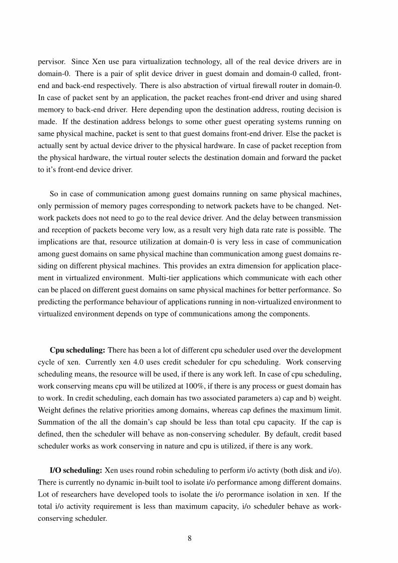
Figure 4.2 shows the current cloudsim class diagram. In our work we have added and modifiedsome classes to add features, 5.1 shows class diagram of cloudsim after some of the featuresare added. In this section, we give details about some classes which are important for ourimplementation.

Figure 4.2: Cloudsim class diagram [4]

Host: This class represents the characteristics of a physical machine. It encapsulates infor-mation of processing unit, main memory, virtualization monitor specification, disk and networkbandwidth. Also information about provisioning policies for cpu, disk, network and main mem-ory to virtual machines are specified in this class.

Vm: This class represents the characteristics of a virtual machines. Information such asprocessing power, main memory, network and disk bandwidth, hosting physical machine are

19

encapsulated. Statistics about the resource consumption by running applications are also repre-sented by this class.

CloudletScheduler: This abstract class defines the policy of cloudlet (applications) ex-ecution. Depending upon the policies cloudlets are executed concurrently or sequentially.CloudletSchedulerTimeShared and CloudletSchedulerSpaceShared are extended classes whichallows applications to execute concurrently and sequentially respectively. CloudletScheduler-DynamicWorkload class derived from CloudletSchedulerTimeShared allows dynamic resourceload generation.

Cloudlet: This class represents the applications running on virtual machines. It encap-sulates the number of instructions to be executed, amount disk transfer to complete the task.Cloudlet class also provides workload generation model, identification of guest virtual machineon which it’s running.

Network topology: This class contains the BRITE format, which represents the communi-cation delay among different entities.

Figure 4.3: Cloudsim sequence diagram [4]

20

Figure 4.3 shows the sequence diagram of cloudsim. At each simulation step, datacen-ter invokes a method called updateVMProcessing to update the virtual machine status of eachphysical host. Current simulation time is sent as input parameter in this method calls. Theneach physical hosts update all the running applications (or cloudlets) status by invoking update-CloudletsProcessing method. From each virtual machine, the least time among all the timesreturned by applications is sent to physical machine. Physical machine in turn returns the leasttime among all the times returned by virtual machines and internally maintains list of virtualmachines having active applications. And using this values returned by the physical hosts,datacenter determines the next update time.

4.3 Extension of Cloudsim

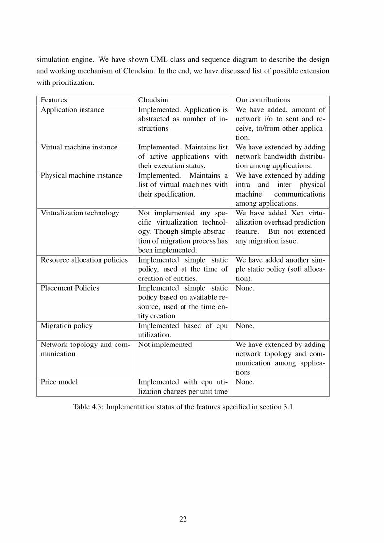
In this section we discuss the limitations of Cloudsim and possible further development of fea-tures. Table 4.3 shows the implementation status of features specified in section 3.1 in Cloudsimand our current work. Also this table shows the limitations of Cloudsim and our work. Some ofmain areas of extension are a) different virtulization overhead prediction b) migration processand it’s overhead c) dynamic resource sharing and placement policies of applications and virtualmachines d) communication among different entities.

Cloudsim has currently implemented simple abstraction of application and virtual machineplacement based on available resource, this policies are static in nature. There is no virtu-alization related issues like a) virtualization overhead b) different types of communication c)migration process overhead, implemented in current version of Cloudsim. Depending upon thevirtualization technology, there can be different features need to implemented. For example, incase of Xen, there are high privileged domain-0 and virtual machine guest domains. All thisspecified features are potential future extension of cloudsim. Since some of the features arepre-requisite for other features, they need to developed first. For example implementing themigration process and it’s overhead on network and cpu usage, communication among applica-tions and virtualization overhead prediction for network i/o should be present.

For implementation of this possible extensions, we would give higher priority to virtual-ization overhead model and migration process over the other possible features. Because thisfeatures are building blocks of virtualization technology and provide more options to developnew policies.

In this chapter, we have discussed the architecture and design of Cloudsim in deatils, withlist of possible extensions of cloudsim. Based on multi-layered architecture, Cloudsim hasthree main components a) user level specification, b) cloudsim components, c) event driven

21

simulation engine. We have shown UML class and sequence diagram to describe the designand working mechanism of Cloudsim. In the end, we have discussed list of possible extensionwith prioritization.

Features Cloudsim Our contributionsApplication instance Implemented. Application is

abstracted as number of in-structions

We have added, amount ofnetwork i/o to sent and re-ceive, to/from other applica-tion.

Virtual machine instance Implemented. Maintains listof active applications withtheir execution status.

We have extended by addingnetwork bandwidth distribu-tion among applications.

Physical machine instance Implemented. Maintains alist of virtual machines withtheir specification.

We have extended by addingintra and inter physicalmachine communicationsamong applications.

Virtualization technology Not implemented any spe-cific virtualization technol-ogy. Though simple abstrac-tion of migration process hasbeen implemented.

We have added Xen virtu-alization overhead predictionfeature. But not extendedany migration issue.

Resource allocation policies Implemented simple staticpolicy, used at the time ofcreation of entities.

We have added another sim-ple static policy (soft alloca-tion).

Placement Policies Implemented simple staticpolicy based on available re-source, used at the time en-tity creation

None.

Migration policy Implemented based of cpuutilization.

None.

Network topology and com-munication

Not implemented We have extended by addingnetwork topology and com-munication among applica-tions

Price model Implemented with cpu uti-lization charges per unit time

None.

Table 4.3: Implementation status of the features specified in section 3.1

22

Chapter 5

Virtualization overhead andcommunication among applications incloudsim

In this chapter, we discuss about the two main features, which are added to cloudsim. Com-munication among different applications and their overhead, can be used in decision makingof different policies like migration and placement policies. We present design details about themodifications and additions of different classes in subsection 5.1. And about overhead utiliza-tion model in subsection 5.2

5.1 Design of communication among entities in cloudsim

Figure 5.1 show the UML class diagram of cloudsim after implementation of the features.Classes shown green and brown colour are the ones added and modified as respectively. Inthis section, we provide details of classes which have been added or modified.

CloudletScheduler: We have added some functions, which supports receiving or transmit-ting data by an application to another. Which are inherited by all the derived scheduler classes.

CloudletSchedulerLogWorkload: This class provides another way of generating work-load for cloudlet applications. It is extended class of CloudletSchedulerTimeShared class. Inmany practical cases we want to create scenario from logs of executed applications statistics.So we have developed this class. Log files with specific format can be given as input of cloudlet.

Cloudlet: Currently, parameter representing network and disk i/o has been added to Cloudletclass. Amount of network data to be sent or received, to or from another entity are encapsulatedto Cloudlet class. To keep the workload generation mechanism same, disk read, disk write,

23

Figure 5.1: Cloudsim UML class diagram after implementation

amount of network data to be received or sent can also use existing workload generation mod-els (maximum utilization, distribution based, random based and log based workload).

DiskProvisioner: This class represents the direct area storage or local storage attachedwith the physical machine. Our simple abstraction of disk is, read and write. Which has sameamount of overhead of irrespective of the position of data. DiskProvisionerSimple is derivedclass, which checks whether there is sufficient availabilty to start an new virtual machine.

Vm: We have added disk and network i/o parameter to Vm class. We have also addedfunctionalities to distribute disk and network bandwidth among applications based on resourceallocation policy. Vm class also additionally implements DiskProvisioner class. While updatingcloudlet execution status, disk and network activity are also taken into account. Since commu-nication is possible between applications residing on same virtual machine or same physicalmachine but on different virtual machines or completely different physical machine, distribu-tion of network bandwidth while maintaining resource allocation policy is quite difficult.

Host: We have added many functionalities to Host class in order to support communicationbetween applications and reporting the overhead due to this i/o activity on behalf of guest virtualmachines. We report the amount of resource utilization at host level to represent domain-0 re-source utilization of Xen hypervisor. Domain-0 overhead for intra and inter physical machinesare different, so at host level total network is divided into four categories a) intra physical ma-chine received b) intra physical machine sent c) inter physical machine received d) inter physical

24

machine sent. Using the provided overhead model, total resource utilization due to network anddisk i/o are reported at host level. One other important addition Host class is the overheadmodel. Domain-0 cpu utilization is predicted using this overhead model.

Figure 5.2: Cloudsim sequence diagram

Figure 5.2 shows the sequence diagram of cloudsim after all the above additions and mod-ifications. As shown in the figure, a new event calculate distribution BW is created, whichdistributes the available bandwidth of a virtual machines among the cloudlets running on thatvirtual machines. Figure 5.3 shows the sequence diagram of distribution of network bandwidthin more details. At virtual machine level depending upon the allocation policy (implementedin CloudletScheduler), total bandwidth is distributed among all the applications, which has net-work data to sent. And then each application sent request for bandwidth reservation to the des-tination application with the calculated amount. Each application which is destination for net-work i/o, reserves the available bandwidth for the connection and replies that reserved amountby reply BW event to the source. If the reserved bandwidth is less than calculated amount at thesource application, this reservation process iterates until either all the applications requirementis fulfilled or no available bandwidth is left.

25

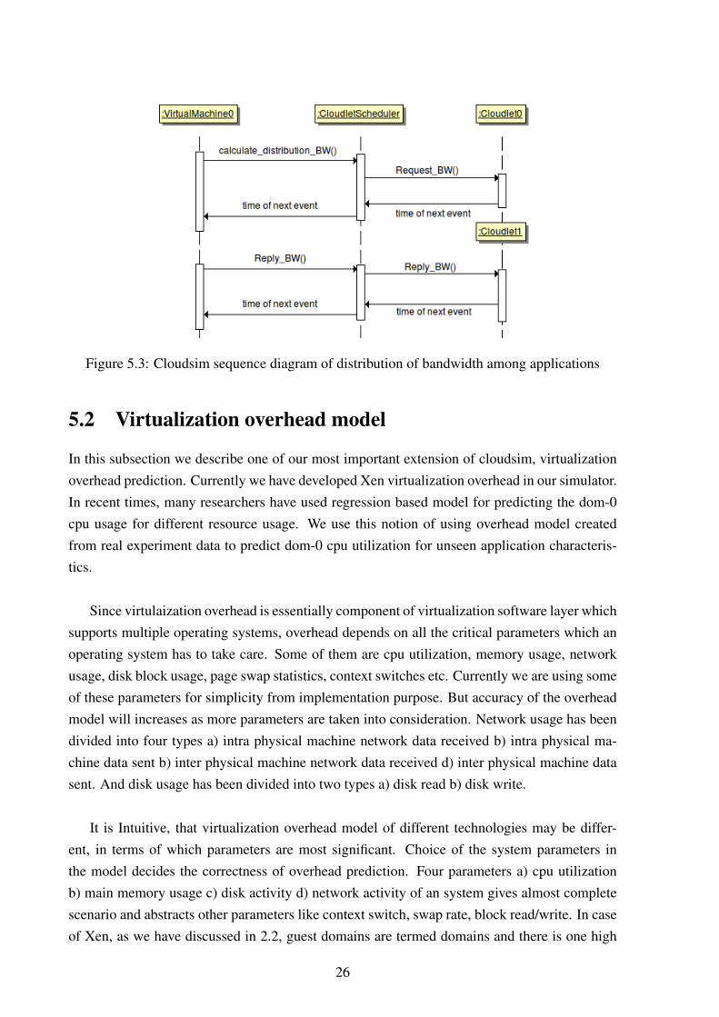
Figure 5.3: Cloudsim sequence diagram of distribution of bandwidth among applications

5.2 Virtualization overhead model

In this subsection we describe one of our most important extension of cloudsim, virtualizationoverhead prediction. Currently we have developed Xen virtualization overhead in our simulator.In recent times, many researchers have used regression based model for predicting the dom-0cpu usage for different resource usage. We use this notion of using overhead model createdfrom real experiment data to predict dom-0 cpu utilization for unseen application characteris-tics.

Since virtulaization overhead is essentially component of virtualization software layer whichsupports multiple operating systems, overhead depends on all the critical parameters which anoperating system has to take care. Some of them are cpu utilization, memory usage, networkusage, disk block usage, page swap statistics, context switches etc. Currently we are using someof these parameters for simplicity from implementation purpose. But accuracy of the overheadmodel will increases as more parameters are taken into consideration. Network usage has beendivided into four types a) intra physical machine network data received b) intra physical ma-chine data sent b) inter physical machine network data received d) inter physical machine datasent. And disk usage has been divided into two types a) disk read b) disk write.

It is Intuitive, that virtualization overhead model of different technologies may be differ-ent, in terms of which parameters are most significant. Choice of the system parameters inthe model decides the correctness of overhead prediction. Four parameters a) cpu utilizationb) main memory usage c) disk activity d) network activity of an system gives almost completescenario and abstracts other parameters like context switch, swap rate, block read/write. In caseof Xen, as we have discussed in 2.2, guest domains are termed domains and there is one high

26

Figure 5.4: Domain-0 and domain-u cpu utilization vs disk read at guest domain

privileged domain called Domain-0. In Xen hypervisor architecture, i/o activity is handled bythe domain-0. And cpu utilization of domain-0 mostly does not depend on guest domain’s cpuutilization. So while creating the virtualization overhead model for Xen, we have only takendisk and network activity into our consideration.

We conducted some simple experiments to show relationship between domain-0’s cpu uti-lization with guest domains i/o activity (both disk and network). Figure 5.4 shows domain-0and domain-u’s cpu utilization against different disk read rate by guest domain applications.Each point in x-axis represent, represent different rate at which disk has been read. And cpuutilization for that at domain-0 and guest domain has been shown in y-axis. Similarly figure 5.5shows the cpu utilization of domain-0 and guest domain against network data rate. As we cansee form both the graphs, domain-0 cpu utilization increases as amount of disk read and totalnetwork i/o increases. This is due to the xen architecture discussed in section 2.2. We havevaried the amount disk read rate from 1 MBps to 80 MBps, and cpu utilization reaches upto30%. While in the network vs domain-0 cpu utilization, we have varied the amount of networkfrom 10 MBps to 160MBps. And the cpu utilization have touched almost 100%, reaching asaturation region. So we can conclude that cpu utilization of domain-0 is highly correlated withi/o (both disk and network) activity. And we have this idea to build the virtualization overheadmodel.

Since domain-0 cpu utilization shows an almost linear relationship with the guest domainsdisk and network activity, we have used linear regression model to represent the overhead uti-

27

Figure 5.5: Domain-0 and domain-u cpu utilization vs network data rate at guset domain

lization model [7]. Shown in Eqn. 5.1

U1dom−0 = c10 + c11 ∗M1

1 + c12 ∗M12 · · ·+ c1j ∗M1

j

U2dom−0 = c20 + c21 ∗M2

1 + c12 ∗M22 · · ·+ c1j ∗M2

j

. . .

(5.1)

Where,

M ji represents the measured value of parameter Mi at time interval j at the guest domain level.

U jdom−0 represents corresponding measured domain-0 cpu utilization at time j.

Assuming c0, c1, c2 . . . cj be the approximated solution for Eqn. 5.1, we can predict the domain-0’s cpu utilization using Eqn. 5.2.

Udom−0 = c0 +

j∑i=1

ci ∗Mi (5.2)

Our representation of virtualization overhead model is shown below.

Dom-0 cpu utilization = Constant + c0 ∗ intra pm data received

+ c1 ∗ intra pm data sent + c2 ∗ inter pm data received

+ c3 ∗ inter pm data sent + c4 ∗ disk read + c5 ∗ disk write

(5.3)

28

To validate this feature, we have created a virtualization overhead model for xen, from realexperiment, done on xen virtualization environment. Steps are a) create the overhead modelfrom experiment data b) using this developed model, predict virtualization overhead on thesame data from which the model is created c) using this developed model, predict virtualizationoverhead on some unseen data. In both last two cases, we calculate the amount of error in pre-diction of the overhead value.

In this chapter, we have discussed the modifications of Cloudsim to implement the featuresand steps of virtualization overhead model creation. We have shown UML class and sequencediagram to describe the modifications of different classes and execution mechanism, after im-plementing the features. Then we have discussed in details, which parameters are chosen forcreating the virtualization overhead model and it’s importance.

29

30

Chapter 6

Verification of virtualization overheadprediction and application abstraction

In this chapter, we discuss some of the features verification process. We mainly focus on virtu-alization overhead prediction. We also conducted small experiment to verify the abstraction ofcloudsim, discussed in 6.2.

6.1 Virtualization overhead

We wanted to verify, whether domain-0 cpu overhead can be predicted and whether that pre-dicted value will have a acceptable small error rate. Steps we followed are as a) create domain-0overhead model as function of network and disk i/o from real experiment data b) use that modelin the simulator c) provide the application characteristics of an real experiment done on samehardware platform and predict the domain-0 cpu utilization d) compare the predicted outputwith the actual domain-0 cpu utilization, to check whether it satisfies an acceptable error limit.Now we discuss the experiment details, used to create domain-0 cpu overhead model.

Aim: is to generate network i/o load by applications running in virtual machines and profil-ing different resource usage at both virtual and physical machine level. Then use this profileddata to create domain-0 cpu overhead model.

Setup: Figure 6.1 shows the setup of first experiment. The physical machines are connectedby a layer-2 switch. Both the physical machines are connected to the NFS server, which hoststhe virtual machine images. Each physical machine hosts a virtual machine. These two physicalmachines have same configuration, Intel Core 2 Quad (Q9550) machines with 2.83 GHz cores,with the Xen 3.3 virtualization environment. Controller and NFS server both non-virtualizedhave 2.60 GHz cores. And the switch operates 100Mbps.

31

Controller unit specifies the workload to be generated, measures the resource usage at differ-ent levels and stores them. As stated first step is to create an overhead model from experimentdata. Whole experiment is divided into multiple small experiment run with varying parameters,each running for almost 60 seconds duration. Average value is taken from this each small 60slong experiment. We have organized the resource usage as shown in table 6.1. Both the virtualmachines host TCP server and client. Any virtual machine wishes to receive network i/o fromother virtual machine, invokes the TCP client specifying amount of bytes. By changing theinterval time of inter-request, data rate has been varied. Data rate has been varied from 10MBpsto 90Mbps by steps of 10Mbps.

Domain-0 Intra-PM Intra-PM Inter-PM Inter-PM disk diskcpu network network network network read write

utilization i/o received i/o sent i/o received i/o sent

Table 6.1: Tabulation of the matrics used for modelling

Figure 6.1: Experiment setup [8]

Result: Using R [11] mathematical tool, we have calculated the value of different coeffi-cients and the created model is shown as below.

Domain-0 cpu utilization =2.45 + 0.0001053 ∗ (intra physical machine received)

+ 0.00000294 ∗ (intra physical machine sent)

+ 0.000001319 ∗ (inter physical machine receive)

+ 0.0000011 ∗ (inter physical machine sent)

+ (−0.01389) ∗ (disk read) − 0.005437 ∗ (disk write)

(6.1)

Now we have used this model shown in Equ. 6.1, in our simulator for prediction of domain-0 cpu utilization. And load generated at application level has been used as input of cloudletcharacteristics. Using the given overhead model and cloudlet characteristics, domain-0 cpu

32

Figure 6.2: Comparison of predicted and actual domain-0 cpu utilization at physical machine 1

utilization has been predicted. Next step we compare the predicted domain-0 cpu utilizationwith actual measured domain-0 cpu utilization. Figure 6.2 and 6.3 shows the predicted andactual measured domain-0 cpu utilization at physical machine 1 and 2 respectively.. Each pointin x-axis represents, the average of an 60 second long experiment’s dom-0 cpu utilization. Iny-axis, the predicted dom-0 cpu utilization by the simulator and actual measured dom-0 cpuutilization is showed. Measured cpu utilization of domain-0 has varied from 0 to 20%, sincemaximum data rate used is 90 Mbps. As we can see the overall difference between measuredand predicted domain-0 cpu utilization is very less. And as the measured dom-0 cpu utilizationincreases, the amount of error also tend to increase. For further clarification on the amount oferror, we have sorted the error with respect to total amount of network i/o.

Figure 6.4(a) and 6.4(b) shows the error in terms of percentage vs total network i/o, at phys-ical machine 1 and 2 respectively. Each point in x-axis represent the amount of network i/o(both sent and received) and in y-axis, the difference between actual and predicted value. Asthe figure shows amount of error is with ± 2%. The error is calculated as the difference betweenmeasured and predicted cpu utilization in terms of %. We can observe that the error remainswithin a small threshold and their is a pattern in the calculated error. This is due to the differentamount of network i/o received and sent. As coefficient for network i/o received and sent hasdifferent values, there will be different predicted dom-0 cpu utilization for same amount of totalnetwork i/o (both sent and received), while varying the amount of data sent and received.

In this section, we have discussed the verification process of virtualization overhead predic-

33

Figure 6.3: Comparison of predicted and actual domain-0 cpu utilization at physical machine 2

(a) Prediction error at physical machine 1 (b) Prediction error at physical machine 2

Figure 6.4: Prediction error of domain-0 cpu utilization on different physcal machines

tion. First we have conducted an experiment in virtualized environment to create an virtualiza-tion overhead model. Then we have used that model to predict the domain-0 cpu utilization andcalculated the error. Our results show that amount of error in prediction is within ± 2%.

34

6.2 Application (cloudlet) characteristics verification

In cloudsim an application (represented as cloudlet) is mainly abstracted as collection of cpuinstructions which are executed based on some distribution or fixed value. As our extension wehave added two more parameters representing amount of data to be sent and received. Belowwe show the current representation of an application (represented as cloudlet) in cloudsim.

1 p u b l i c C l o u d l e t (2 f i n a l i n t c l o u d l e t I d ,3 f i n a l long c l o u d l e t L e n g t h ,4 f i n a l i n t pesNumber ,5 f i n a l long c l o u d l e t F i l e S i z e ,6 f i n a l long c l o u d l e t O u t p u t S i z e ,7 f i n a l U t i l i z a t i o n M o d e l u t i l i z a t i o n M o d e l C p u ,8 f i n a l U t i l i z a t i o n M o d e l u t i l i z a t i o n M o d e l R a m ,9 f i n a l U t i l i z a t i o n M o d e l u t i l i z a t i o n M o d e l B w ,

10 f i n a l long sendDataLeng th ,11 f i n a l long r e c e i v e D a t a L e n g t h )1213 P a r a m e t e r s :14 c l o u d l e t I d t h e un iqu e ID of t h i s C l o u d l e t15 c l o u d l e t L e n g t h t h e l e n g t h o r s i z e ( i n MI ) o f t h i s c l o u d l e t t o be

e x e c u t e d i n a P o w e r D a t a c e n t e r16 c l o u d l e t F i l e S i z e t h e f i l e s i z e ( i n byte ) o f t h i s c l o u d l e t BEFORE

s u b m i t t i n g t o a P o w e r D a t a c e n t e r17 c l o u d l e t O u t p u t S i z e t h e f i l e s i z e ( i n byte ) o f t h i s c l o u d l e t AFTER

f i n i s h e x e c u t i n g by a P o w e r D a t a c e n t e r18 pesNumber t h e pes number19 u t i l i z a t i o n M o d e l C p u t h e u t i l i z a t i o n model cpu20 u t i l i z a t i o n M o d e l R a m t h e u t i l i z a t i o n model ram21 u t i l i z a t i o n M o d e l B w t h e u t i l i z a t i o n model bw22 sendDa taLeng th amount o f d a t a t o s e n t23 r e c e i v e D a t a L e n g t h amount o f d a t a t o r e c e i v e

We wanted to verify, how much credibility is assured by abstracting an application as num-ber of instructions. How to profile an application in terms of cpu instructions and use that valuein simulator? To validate the abstraction of application, we have used ”time” command, whichreports the amount cpu time executed by an application. The definition of cpu time is as follows

cpu time = no of instructions ∗ cycles/instruction ∗ 1/(cycles/second of the processing unit)(6.2)

Number of cycles to execute an instruction remains same in same architecture, while varyingthe processing power of the cpu. This means if two physical machines both have X86 archi-tecture in nature, but one has double processing power than the other one, still cycles needed

35

to execute an particular instruction remains same. So in the above equation, both number ofinstructions and cycles/instruction remains same for same architecture and same application.Using the ”time” command we get the cpu time and form hardware configuration, informationabout the cpu processing power is available. Using this two values, we get value of number ofinstruction * cycles/instructions (or cycles). Now since across same architecture cycles/instruc-tion is constant, we can simply abstract number of instruction * cycles/instructions as numberof instruction without introducing any error. Or we can simply assume for every instructioncycles/inst is 1, thus number of instructions * cycles/instructions (or cycles) become number ofinstruction only. Now we discuss a simple experiment to verify, that number of cycles neededto to execute an application remains same across physical machines with same architecture.

Aim: is to verify that no of instructions * cycles/instructions (or cycles) remains almost con-stant for an application in different physical machines (different hardware specification) withsame architecture.

Setup: C program which calculates the n-th Fibonacci number by using recursion, wheren is given as input. Three different physical machines, with X86 architecture in nature withdifferent processing power.

Measurement: We have measured the cpu time of program on each machine and collectedspecification about the cpu. Table 6.2 shows the details of a) physical cpu specification b) out-put of time command and c) number of cycles (or number of instructions * cycles/instruction).Command ”time” shows the total cpu time in three parts a) real time b) user time c) sys time.As expected the total amount of time taken to complete the task reduces, as processing powerof physical machines increases.

cpu real time user time sys time cyclesphysical machine 2 1.60GHz 5m24.273s 5m19.844s 0m0.672s 1031.624GHzphysical machine 1 2.20GHz 3m51.619s 3m51.594s 0m0.000s 1019.0686GHzphysical machine 0 2.33GHz 3m38.488s 3m38.226s 0m0.232s 1018.08418GHz

Table 6.2: Experimental evaluation of application abstraction

Conclusion: As we can see, there is slight difference in number of cycles on differentphysical machines because of the different number of available cache, register and low levelcharacteristics of the operating system. From this result, we can safely use number of cycles, asnumber of instructions needed to complete execution. Since number of instructions and num-ber of cycles needed to execute those instructions can be mapped easily, we can use anyone ofthese two values, ensuring that same parameter is used across the whole setup. Currently for

36

simplification, we have directly used number of cycles as number of instructions. SimpleScalar[9] is a system software which is built for further detailed application performance analysis.

In this chapter, we have verified the virtualization overhead prediction and application char-acteristics by experimental evaluation. The amount of error in prediction remains within a rangeof ± 2%. And we can use both number of instructions or number of cycles as abstraction ofapplications, ensuring that same parameter is used across the whole setup.

37

38

Chapter 7

Correctness and capabilities of cloudsim

In this chapter, we discuss different deterministic test cases for the added features and simpleexperiment using cloudsim showing the capability of the simulator. Test cases for the featurecommunication among applications is discussed below. These test cases are used for checkingthe correctness of the simulator, while adding new features to the simulator. In the simpleexperiment, we have shown how to develop a resource allocation policy, measure differentresource utilization and draw a conclusion.

7.1 Test cases of communication among applications

In this section we specific different test cases for communication among application under dif-ferent system configurations and input characteristics. We vary the setup of the virtual machineplacement and application characteristics to verify the correctness of the communication fea-ture.

7.1.1 Communication among two applications running on different phys-ical machine

Figure 7.1 shows the setup consisting application, virtual machines and physical machines. Twophysical machines with same specification, hosts one virtual machine each. Application 0 run-ning on virtual machine 0 sends network traffic to application 1 running on physical machine 1.

GoalWe are testing a) whether exact same amount of data sent and received b) Application uses max-imum available bandwidth at the virtual machine, on which it is running c) there is specifiedpropagation delay between the data sent and received.

Setup

39

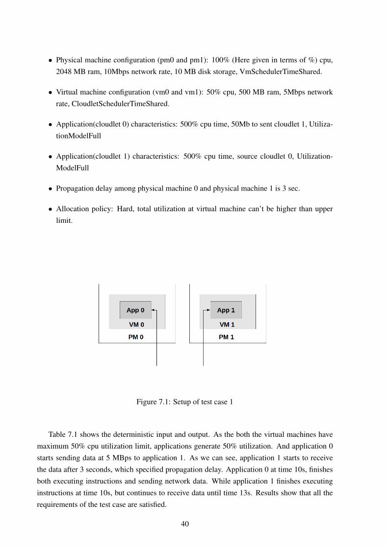
• Physical machine configuration (pm0 and pm1): 100% (Here given in terms of %) cpu,2048 MB ram, 10Mbps network rate, 10 MB disk storage, VmSchedulerTimeShared.

• Virtual machine configuration (vm0 and vm1): 50% cpu, 500 MB ram, 5Mbps networkrate, CloudletSchedulerTimeShared.

• Application(cloudlet 0) characteristics: 500% cpu time, 50Mb to sent cloudlet 1, Utiliza-tionModelFull

• Application(cloudlet 1) characteristics: 500% cpu time, source cloudlet 0, Utilization-ModelFull

• Propagation delay among physical machine 0 and physical machine 1 is 3 sec.

• Allocation policy: Hard, total utilization at virtual machine can’t be higher than upperlimit.

Figure 7.1: Setup of test case 1

Table 7.1 shows the deterministic input and output. As the both the virtual machines havemaximum 50% cpu utilization limit, applications generate 50% utilization. And application 0starts sending data at 5 MBps to application 1. As we can see, application 1 starts to receivethe data after 3 seconds, which specified propagation delay. Application 0 at time 10s, finishesboth executing instructions and sending network data. While application 1 finishes executinginstructions at time 10s, but continues to receive data until time 13s. Results show that all therequirements of the test case are satisfied.

40

App 0 App 1time (sec) cpu % data received data sent cpu % data received data sent

1.0 50.0 0.0 5000000.0 50.0 0.0 0.02.0 50.0 0.0 5000000.0 50.0 0.0 0.03.0 50.0 0.0 5000000.0 50.0 0.0 0.04.0 50.0 0.0 5000000.0 50.0 5000000.0 0.05.0 50.0 0.0 5000000.0 50.0 5000000.0 0.06.0 50.0 0.0 5000000.0 50.0 5000000.0 0.07.0 50.0 0.0 5000000.0 50.0 5000000.0 0.08.0 50.0 0.0 5000000.0 50.0 5000000.0 0.09.0 50.0 0.0 5000000.0 50.0 5000000.0 0.0

10.0 50.0 0.0 5000000.0 50.0 5000000.0 0.011.0 0.0 0.0 0.0 0.0 5000000.0 0.012.0 0.0 0.0 0.0 0.0 5000000.0 0.013.0 0.0 0.0 0.0 0.0 5000000.0 0.014.0 0.0 0.0 0.0 0.0 0.0 0.0

Table 7.1: Test case: communication among two applications running on different physicalmachine

7.1.2 Multiple communications among applications running on differentphysical machine

Figure 7.2 shows the application, virtual machines and physical machines. Two physical ma-chines with same configuration hosts one virtual machine each. Each virtual machine, in turnruns two applications. Both application 0 and application 2 running on virtual machine 0 senddata to application 1 and application 3 respectively.

Goal:We are testing a) whether exact same amount of data sent and received b) Application usesmaximum available bandwidth at the virtual machine c) there is specified propagation delaybetween the data sent and received d) resource utilization follows work-conserving approach e)equal resource sharing.Common setup


• Virtual machine configuration (vm0 and vm1): 50%cpu, 500 MB ram, 5Mbps networkrate, CloudletSchedulerTimeShared.


41






• Allocation policy: Hard, total utilization at virtual machine can’t be higher than upperlimit.

Table 7.2 shows the deterministic input and output of test case 2. As both both virtualmachines can use maximum 50% of cpu utilization, applications running on them share thisamount. Application 0 and application 2 both utilize 25% cpu to execute their instructions,so resource is shared equally among the applications. As we can see, application 2 has lessamount of data to send compared to application 0, application 2 finishes early. At time 10.0s,application 2 finishes executing instructions and sending data. As a result, application 0 usestotal available bandwidth for sending the data and sends at rate of 5Mbps. Since the propagationdelay among physical machines are 3s, application 3 finishes receiving data at time 13s. Andapplication 1 uses the total available bandwidth and receives at rate of 5Mbps. So this showsthe resource sharing follows work-conserving approach. Result shows that all the requirementof test case are fulfilled.

42

App 0 App 1 App 2 App 3data data cpu % data data data data data data

time cpu % received sent cpu % received sent cpu % received sent cpu % received sent1.0 25.0 0.0 2500000.0 25.0 0.0 0.0 25.0 0.0 2500000.0 25.0 0.0 0.02.0 25.0 0.0 2500000.0 25.0 0.0 0.0 25.0 0.0 2500000.0 25.0 0.0 0.03.0 25.0 0.0 2500000.0 25.0 0.0 0.0 25.0 0.0 2500000.0 25.0 0.0 0.04.0 25.0 0.0 2500000.0 25.0 2500000.0 0.0 25.0 0.0 2500000.0 25.0 2500000.0 0.05.0 25.0 0.0 2500000.0 25.0 2500000.0 0.0 25.0 0.0 2500000.0 25.0 2500000.0 0.06.0 25.0 0.0 2500000.0 25.0 2500000.0 0.0 25.0 0.0 2500000.0 25.0 2500000.0 0.07.0 25.0 0.0 2500000.0 25.0 2500000.0 0.0 25.0 0.0 2500000.0 25.0 2500000.0 0.08.0 25.0 0.0 2500000.0 25.0 2500000.0 0.0 25.0 0.0 2500000.0 25.0 2500000.0 0.09.0 25.0 0.0 2500000.0 25.0 2500000.0 0.0 25.0 0.0 2500000.0 25.0 2500000.0 0.010.0 25.0 0.0 2500000.0 25.0 2500000.0 0.0 25.0 0.0 2500000.0 25.0 2500000.0 0.011.0 0.0 0.0 4999999.0 0.0 2500000.0 0.0 0.0 0.0 0.0 0.0 2500000.0 0.012.0 0.0 0.0 4999999.0 0.0 2500000.0 0.0 0.0 0.0 0.0 0.0 2500000.0 0.013.0 0.0 0.0 4999999.0 0.0 2500000.0 0.0 0.0 0.0 0.0 0.0 2500000.0 0.014.0 0.0 0.0 4999999.0 0.0 4999999.0 0.0 0.0 0.0 0.0 0.0 0.0 0.015.0 0.0 0.0 4999999.0 0.0 4999999.0 0.0 0.0 0.0 0.0 0.0 0.0 0.016.0 0.0 0.0 4999999.0 0.0 4999999.0 0.0 0.0 0.0 0.0 0.0 0.0 0.017.0 0.0 0.0 0.0 0.0 4999999.0 0.0 0.0 0.0 0.0 0.0 0.0 0.018.0 0.0 0.0 0.0 0.0 4999999.0 0.0 0.0 0.0 0.0 0.0 0.0 0.019.0 0.0 0.0 0.0 0.0 4999999.0 0.0 0.0 0.0 0.0 0.0 0.0 0.020.0 0.0 0.0 0.0 0.0 0.0 0.0 0.0 0.0 0.0 0.0 0.0 0.0

Table 7.2: Test case: a pair of communication among applications running on different physicalmachine

7.1.3 Communication among applications with soft resource allocationpolicy at physical host level

Figure 7.3 shows the setup of application, virtual machines and physical machine. In this testcase we are changing resource allocation policy at the physical machine level. If allocation pol-icy at host level is soft, the resource scheduling works as work conserving. Any virtual machinecan acquire resources more thhan it’s maximum limit, if others are not using their share. In thiscase, both physical machines host two virtula machines each. And each virtual machine hostone application. Application 0 running on virtual machine 0 sends data to application 1 runningon virtual machine 1. And similarly application 2 is sending data to application 3. Differencewith test case 2 described in subsection 7.1.2 is that here each application is running on separatevirtual machines and resource allocation policy specified at the physical host level is important.

GoalWe are testing a) allocation policy at physical machine level b) resource sharing among virtualmachines and applications.

Setup


• Virtual machine configuration (vm0, vm1, vm2 and vm3): 50%cpu, 500 MB ram, 5Mbpsnetwork rate, CloudletSchedulerTimeShared.

43







• Allocation policy: Soft, total utilization at virtual machine can be higher than upper limit.

Table 7.3 shows the deterministic input and output of test case 3. As all the virtual machinescan have maximum 50% cpu utilization, applications running on this virtual machines usesthis total availability. Since virtual machines are configured to use 2.5Mbps, applications senddata at 2.5Mbps. At time 10s, application 2 running on virtual machine 2, finishes sendingamount of data and completes the execution. Since we have set resource allocation as softin physical machine level, application running on virtual machine 0 uses the total availablenetwork bandwidth at physical host level and sends data at 5Mbps. There is 3s delay betweensending and receiving data by applications. This results show that all the requirement of the testcase are fulfilled.

44

App 0 App 1 App 2 App 3data data cpu % data data data data data data

time cpu % received sent cpu % received sent cpu % received sent cpu % received sent1.0 50.0 0.0 2500000.0 50.0 0.0 0.0 50.0 0.0 2500000.0 50.0 0.0 0.02.0 50.0 0.0 2500000.0 50.0 0.0 0.0 50.0 0.0 2500000.0 50.0 0.0 0.03.0 50.0 0.0 2500000.0 50.0 0.0 0.0 50.0 0.0 2500000.0 50.0 0.0 0.04.0 50.0 0.0 2500000.0 50.0 2500000.0 0.0 50.0 0.0 2500000.0 50.0 2500000.0 0.05.0 50.0 0.0 2500000.0 50.0 2500000.0 0.0 50.0 0.0 2500000.0 50.0 2500000.0 0.06.0 0.0 0.0 2500000.0 0.0 2500000.0 0.0 0.0 0.0 2500000.0 0.0 2500000.0 0.07.0 0.0 0.0 2500000.0 0.0 2500000.0 0.0 0.0 0.0 2500000.0 0.0 2500000.0 0.08.0 0.0 0.0 2500000.0 0.0 2500000.0 0.0 0.0 0.0 2500000.0 0.0 2500000.0 0.09.0 0.0 0.0 2500000.0 0.0 2500000.0 0.0 0.0 0.0 2500000.0 0.0 2500000.0 0.010.0 0.0 0.0 2500000.0 0.0 2500000.0 0.0 0.0 0.0 2500000.0 0.0 2500000.0 0.011.0 0.0 0.0 4999999.0 0.0 2500000.0 0.0 0.0 0.0 0.0 0.0 2500000.0 0.012.0 0.0 0.0 4999999.0 0.0 2500000.0 0.0 0.0 0.0 0.0 0.0 2500000.0 0.013.0 0.0 0.0 4999999.0 0.0 2500000.0 0.0 0.0 0.0 0.0 0.0 2500000.0 0.014.0 0.0 0.0 4999999.0 0.0 4999999.0 0.0 0.0 0.0 0.0 0.0 0.0 0.015.0 0.0 0.0 4999999.0 0.0 4999999.0 0.0 0.0 0.0 0.0 0.0 0.0 0.016.0 0.0 0.0 4999999.0 0.0 4999999.0 0.0 0.0 0.0 0.0 0.0 0.0 0.017.0 0.0 0.0 0.0 0.0 4999999.0 0.0 0.0 0.0 0.0 0.0 0.0 0.018.0 0.0 0.0 0.0 0.0 4999999.0 0.0 0.0 0.0 0.0 0.0 0.0 0.019.0 0.0 0.0 0.0 0.0 4999999.0 0.0 0.0 0.0 0.0 0.0 0.0 0.020.0 0.0 0.0 0.0 0.0 0.0 0.0 0.0 0.0 0.0 0.0 0.0 0.0

Table 7.3: Test case: a pair of communication among applications running on different physicalmachine, with allocation policy soft at the physical machine level

7.2 Experiment using cloudsim

In this section we discuss about a simple experiment showing the capabilities of cloudsim. Inthis experiment, we varied the resource sharing policy and reported the resource utilization atvirtual and phsyical machine level. We want to test, the effect of resource utilization at virtualand physical machine level, varying the resource allocation policy. This helps to determine theaverage usage of resource, application execution time-length, difference between demand andavailability of resource. We will run same application in both cases with different allocationpolicy.

In the experiment setup, there is only one physical machine and four virtual machines run-ning on that host. Each virtual machine has been configured with equal amount of physical hostresource share. Applications running on virtual machines have only instructions to completethe execution. There is no communication among the different applications.

Goal:We want to measure the different resource utilization at both virtual and physical machines,depending upon the resource allocation policy used. At virtual machine level, the amount ofdemand and available resource usage. And at physical level, total amount of resource utilizationcomprising all the virtual machines.

Setup:

• 4 virtual machines in a single physical host

45

• Physical machine configuration: 1000 inst/sec (processing), 1024 MB (RAM), 20 MB/sec(diks i/o), 20 MB/sec (network i/o)

• Virtual machine configuration: 250 inst/sec (processing), 256 MB (RAM), 5 MB/sec(diks i/o), 5 MB/sec (network i/o)

• Application characteristics: log based model

• Resource allocation policy: hard and soft allocation policy

(a) Virtual machine1 (b) Virtual machine2

(c) Virtual machine3 (d) Virtual machine4

Figure 7.4: Resource requirement and availability in soft vs hard allocation policy in virtualmachines

Figure 7.4 and 7.5 show the demand, availability of resource at different virtual machinesand physical host level, with hard and soft allocation policy respectively. Each point in x-axisrepresent the time (in seconds). And each point in y-axis represnt the resource utilization (in%). Figure 7.4(a) shows the availability of resource at virtual machine 1. Which is limited to25% in case of hard allocation, as a result the difference between requirement and availabilityis high compared to soft allocation. In case of using soft allocation, we can see that amount ofavailable resource is higher than hard allocation. As a result, we can conclude that using soft

46

Figure 7.5: Total resource utilization in soft vs hard allocation in physical machines

allocation, applications requirement is fulfilled better than using hard allocation.

Figure 7.5 shows the total resource utilization at the physical host level. In soft allocation,the availability of resources among all the virtual machines is higher than hard allocation. Wecan see, that even if there is demand of 160%, hard allocation only allows upto 70% whereassoft allocation allows upto 100%. As a result we can see, resource utilization is better at physi-cal host compared in soft allocation. Further from this experimental data, we can use calculateddeficit amount to determine amount service level agreement violation.

In this chapter, we have discussed different test cases for checking correctness and simpleexperiment to show the capability of cloudsim. All the test cases provide a set of correctnesscriteria under different experiment setup, with deterministic input and output set. Experimentwith resource allocation shows the potential usage of testing new policies with a large setupusing this simulator.

47

48

Chapter 8

Summary and Conclusions

In this report, we present the design and verification of two developed features in cloudsim, a)Xen virtualization overhead prediction and b) communication between applications. Also wehave discussed correctness and capabilities of cloudsim, by providing different test cases andconducting a simple experiment.

We have conducted simple experiments to chose the correct parameters for creation of thevirtualization overhead model. Using experimental data in virtualized environment, we havecreated the virtualization overhead model and calculated the amount of error in prediction. Re-sult shows that amount of error in predicting the virtualization overhead remains within a rangeof ± 2%. Also an application can be abstracted by number of instructions or number of cyclesneeded to complete the execution.

Currently we have mainly focused on Xen virtualization technology in predicting the virtu-alization overhead and communication among applications. This same procedure can be imple-mented for KVM virtualization technology. Other important potential extensions of Cloudsimare a) migration process, it’s overhead and migration policy b) placement and resource alloca-tion policies.

49

50

Chapter 9

Appendix

9.1 Configuration and input files of cloudsim

In this section we describe the XML representation of the system configuration and differentinput specifications used in cloudsim.

9.1.1 System configuration

Here we describe the system configuration of data center characteristics, data center broker, net-work topology. Data center in turn represents all the physical machine and their characteristics.Data center is represented by unique id (name), virtual machine allocation policy (VmAlloca-tionPolicy), scheduling interval (schedulingInterval) and characteristics of physical machines(DatacenterCharacteristic). Common information about physical hosts are given as a) architec-ture (architecture) b) operating system (os) c) virtual machine monitor or hypervisor (vmm) d)time zone (timeZone) e) cost of processing unit or cpu usage (costPerSec) f) cost of main mem-ory usage (costPerMem) g) cost of storage usage (costPerStorage) h) cost of bandwidth usage(costPerBw). Each physical host (PhysicalHost) is represented by a) unique identifier (ID) b)main memory size (Ram) c) bandwidth (Bw) d) storage (Storage) e) vm scheduler (VmSched-uler) f) list of processing unit (PeList) and virtualization overhead model.

‘Overhead model represents different parameters and their coefficient values. For examplehere physical machine with id 0, has seven parameters a) constant (const) b) intra physicalmachine network i/o received (intra pm rx) c) intra physical machine network i/o sent (in-tra pm tx) d) inter physical machine network i/o received (inter pm rc) e) inter physical ma-chine network i/o sent (inter pm tx) f) disk read (disk read) g) disk write (disk write).

Cloudlet broker is represented by an unique id (Name). Network topology (Network topology)is represented by BRITE format. And then each physical host is mapped to the nodes specified

51

in BRITE format. This representation contains a) path name containing the BRITE format fileb) list of entries of format ¡physical host, node id¿.

1 <D a t a c e n t e r s>2 <D a t a c e n t e r>3 <name>D a t a c e n t e r 0< / name>4 <V m A l l o c a t i o n P o l i c y>V m A l l o c a t i o n P o l i c y S i m p l e< / V m A l l o c a t i o n P o l i c y>5 < s c h e d u l i n g I n t e r v a l>1< / s c h e d u l i n g I n t e r v a l>6 <D a t a c e n t e r C h a r a c t e r i s t i c>7 <a r c h i t e c t u r e>x86< / a r c h i t e c t u r e>8 <os>Linux< / os>9 <vmm>Xen< /vmm>

10 <t imeZone>1 0 . 0< / t imeZone>11 <c o s t P e r S e c>3 . 0< / c o s t P e r S e c>12 <costPerMem>0 . 0< / costPerMem>

13 <c o s t P e r S t o r a g e>0 .001< / c o s t P e r S t o r a g e>14 <cos tPerBw>0 . 0< / cos tPerBw>

15 16 <Id>017 <Ram>2048< / Ram>18 <Bw>10000000< /Bw> <!−− 10ˆ7 bps −−>19 <S t o r a g e>1000000< / S t o r a g e>20 <VmScheduler>VmSchedulerTimeShared< / VmScheduler>21 22 <Mips i n s t =” 100 ”>< / Mips>23 24 <Technology name=” xen ”>25 <c o n s t>1< / c o n s t>26 . 00000427 . 00000528 . 000000429 . 000000530 <d i s k r e a d>. 0000004< / d i s k r e a d>31 <d i s k w r i t e>. 0000004< / d i s k w r i t e>32 < / Technology>33 34 < / D a t a c e n t e r C h a r a c t e r i s t i c>35 < / D a t a c e n t e r>36 < / D a t a c e n t e r s>3738 39 <Broker>40 <Name>Broker< / Name>41 < / Broker>42 4344 <N e t w o r k t o p o l o g y>

52

45 < f i l e> / home / k r i s h n a / workspace / c louds im −2 .1 / examples / o rg / c l o u d b u s /c l o u ds i m / examples / ne twork / t o p o l o g y . b r i t e< / f i l e>

46 <nodes>47 <node p h y s i c a l h o s t =” 0 ” n o d e i d =” 1 ”>< / node>48 <node p h y s i c a l h o s t =” 1 ” n o d e i d =” 2 ”>< / node>49 < / nodes>50 < / N e t w o r k t o p o l o g y>

9.1.2 Input specification

In this section, we describe the components like virtual machine and application characteristics,which are more frequently changed in a simulation setup. Virtual machines (VirtualMachine)are represented by a) unique id (ID) b) number of assigned processing units or cpu (pesNum-ber) c) size of the image (size) d) processing power of each cpu (mips) e) size of assigned mainmemory (ram) f) type of hypervisor or vmm, on which this virtual machine will run (vmm) andg) cloudlet scheduler type (CloudletScheduler).

Applications (or cloudlets) are represented by a) unique id (Id) b) number of instructionsto be executed (Length) c) number of assigned processing units (pesNumber) d) the input filesize of this Cloudlet before execution (FileSize) e) the output file size of this Cloudlet afterexecution (OutputSize) f) amount of bytes to be sent (DatatoSend) g) amount of data to be re-ceived (DatatoReceive) h) utilization model of cpu, memory and bandwidth (UtilizationModel)i) destination application id which receives the network i/o (Destination cloudlet) and j) sourceapplication id from which data is received (Source cloudlet). Each virtual machine is assignedwith a list of applications id’s, which will be executed on it [?].

12 <V i r t u a l M a c h i n e s>3 <V i r t u a l M a c h i n e>4 <Id>05 <pesNumber>1< / pesNumber>6 <s i z e>10000< / s i z e>7 <mips>50< / mips>8 <ram>500< / ram>

9 <bw>5000000< / bw>10 <vmm>xen< /vmm>11 <C l o u d l e t S c h e d u l e r>C l o u d l e t S c h e d u l e r T i m e S h a r e d< / C l o u d l e t S c h e d u l e r>12 < / V i r t u a l M a c h i n e>13 < / V i r t u a l M a c h i n e s>1415 <C l o u d l e t s>16 <C l o u d l e t>

53

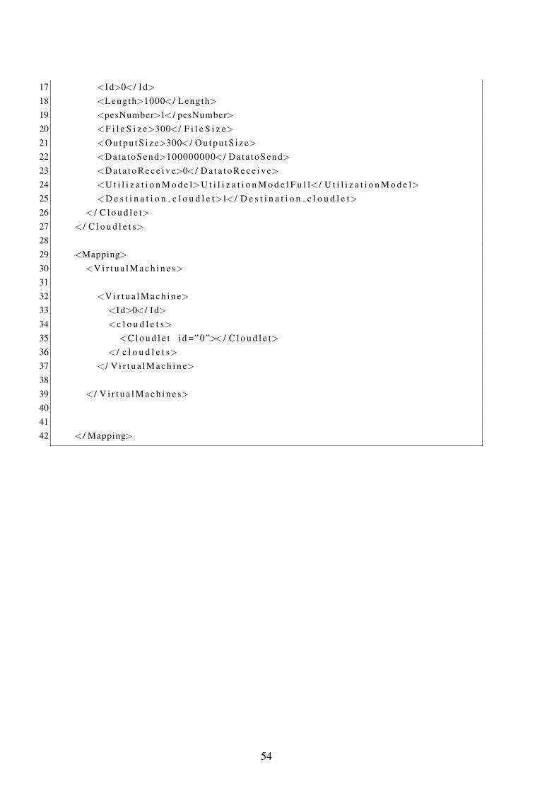
17 <Id>018 <Length>1000< / Length>19 <pesNumber>1< / pesNumber>20 <F i l e S i z e>300< / F i l e S i z e>21 <O u t p u t S i z e>300< / O u t p u t S i z e>22 <Data toSend>100000000< / Da ta toSend>23 <D a t a t o R e c e i v e>0< / D a t a t o R e c e i v e>24 U t i l i z a t i o n M o d e l F u l l25 <D e s t i n a t i o n c l o u d l e t>1< / D e s t i n a t i o n c l o u d l e t>26 < / C l o u d l e t>27 < / C l o u d l e t s>2829 <Mapping>30 <V i r t u a l M a c h i n e s>3132 <V i r t u a l M a c h i n e>33 <Id>034 <c l o u d l e t s>35 <C l o u d l e t i d =” 0 ”>< / C l o u d l e t>36 < / c l o u d l e t s>37 < / V i r t u a l M a c h i n e>3839 < / V i r t u a l M a c h i n e s>404142 < / Mapping>

54

Bibliography

[1] Michael Armbrust, Armando Fox, Rean Griffith, Anthony D. Joseph, Randy H.Katz, An-drew Konwinski, Gunho Lee, David A. Patterson, Ariel Rabkin, IonStoica, and MateiZaharia. Above the clouds: A berkeley view of cloud computing. Technical ReportUCB/EECS-2009-28, EECS Department, University of California, Berkeley, Feb 2009.

[2] Barham, Paul and Dragovic, Boris and Fraser, Keir and Hand, Steven and Harris, Timand Ho, Alex and Neugebauer, Rolf and Pratt, Ian and Warfield, Andrew. Xen and theart of virtualization. In SOSP ’03: Proceedings of the nineteenth ACM symposium on Op-

erating systems principles, 2003, 1-58113-757-5, 164–177, Bolton Landing, NY, USA,http://doi.acm.org/10.1145/945445.945462, ACM, New York, NY, USA.

[3] Kernel Based Virtual Machine. Website. http://www.linux-kvm.org.

[4] Rodrigo N. Calheiros, Rajiv Ranjan, Anton Beloglazov, Cesar A. F. De Rose, and Rajku-mar Buyya. CloudSim: A Toolkit for Modeling and Simulation of Cloud Computing En-vironments and Evaluation of Resource Provisioning Algorithms. Software: Practice andExperience, ISSN: 0038-0644, Wiley Press, New York, USA, 2010 (in press, accepted onJune 14, 2010).

[5] Rajkumar Buyya, Rajiv Ranjan and Rodrigo N. Calheiros. Modeling and Simulation ofScalable Cloud Computing Environments and the CloudSim Toolkit: Challenges and Op-portunities. In Proceedings of the 7th High Performance Computing and Simulation Con-

ference (HPCS 2009, ISBN: 978-1-4244-4907-1, IEEE Press, New York, USA), Leipzig,Germany, June 21-24, 2009.

[6] David Chisnall The Definitive Guide to the Xen Hypervisor (Prentice Hall Open SourceSoftware Development Series). Prentice Hall PTR, Upper Saddle River, NJ, USA, 2007.

[7] K. Ozonat T. Wood, L. Cherkasova and P. Shenoy. Profiling and Modeling Resource Usageof Virtualized Applications. In Middleware ’08: Proceedings of the 9th ACM/IFIP/USENIX

International Conference on Middleware, pages 366-387. Springer-Verlag New York, Inc,2008.

55

[8] Sujesha Sudevalayam and Purushottam Kulkarni. Affinity-aware Modeling of CPU Usagefor Provisioning Virtualized Applications. In Proceedings of IEEE Cloud 2011, the 4thInternational Conference on Cloud Computing, Washington DC, USA.

[9] D. Burger, T.M. Austin. The SimpleScalar Tool Set, Version 2.0, Technical Report, Com-puter Science Department, University of Wisconsin-Madison, June 1997

[10] The BRITE Output Format. Website. http://www.cs.bu.edu/brite/user_manual/node29.html

[11] M. Maechler. robustbase: Basic robust statistics. Website. http://cran.

r-project.org/web/packages/robustbase/index.html.

[12] A. Legrand, L. Marchal, and H. Casanova. Scheduling distributed applications: the Sim-Grid simulation framework. Proceedings of the 3rd IEEE/ACM International Symposium

on Cluster Computing and the Grid, 2003.

[13] R. Buyya and M. Murshed. GridSim: A Toolkit for the Modeling and Simulation ofDistributed Resource Management and Scheduling for Grid Computing. Concurrency and

Computation: Practice and Experience, 14(13-15), Wiley Press, Nov.-Dec., 2002

56

Documents

CLOUD COMPUTING SIMULATION