Embed Size (px)
Citation preview

Closed Streamlines in FlowVisualizationVom Fa hberei h Informatikder Universit�at Kaiserslauternzur Erlangung des akademis hen Grades"Doktor der Naturwissens haften\(Dr. rer. nat.)genehmigte DissertationvonDipl.-Inform. Thomas Wis hgollKaiserslautern25. Juni 20021. Beri hterstatter: Prof. Dr. Hans Hagen2. Beri hterstatter: Prof. Dr. Eduard Gr�ollerVorsitzender der Promotionskommission: Prof. Dr. Otto MayerDekan: Prof. Dr. J�urgen AvenhausDatum der wissens haftli hen Ausspra he: 18. Oktober 2002

ii
Department of Computer S ien e, University of Kaiserslautern, Germany

Closed Streamlines in Flow Visualization iii
To my parents
Department of Computer S ien e, University of Kaiserslautern, Germany

iv
Department of Computer S ien e, University of Kaiserslautern, Germany

Closed Streamlines in Flow Visualization vOne thing I have learned in a long life: that all our s ien e,measured against reality, is primitive and hildlike and yet itis the most pre ious thing we have.Albert Einstein (1879{1955)
A knowledgmentsI want to thank all the people who helped me to a omplish this work during the lastthree and a half years. I thank my advisor, Prof. Dr. Hans Hagen, for giving me theopportunity to work on this interesting topi and letting me join international meetingsand onferen es in order to get in tou h with other s ientists. I also thank Dr. GerikS heuermann for providing me with some starting points and helping me throughoutthis work. Without him this work would not have been possible.During my studies I was glad to have su h helpful olleagues like Holger Burba hand Xavier Tri o he. I also thank all the members of the proje t FAnToM who providedthe basis for my implementations. A spe ial thank goes to Mady Gruys for reating apositive atmosphere and helping me in all non-s ienti� problems. Additionally, I wantto thank Inga S heler for proof reading this work and helping me to get it printed. Lastbut not least I would like to thank my parents who always supported me over the years.Part of this work was funded by DFG (Deuts he Fors hungsgemeins haft) and LandRheinland-Pfalz, Germany.
Department of Computer S ien e, University of Kaiserslautern, Germany

vi
Department of Computer S ien e, University of Kaiserslautern, Germany
Closed Streamlines in Flow Visualization vii
Abstra tVe tor �elds o ur in many of the problems in s ien e and engineering. In ombustionpro esses, for instan e, ve tor �elds des ribe the ow of the gas. This pro ess an beenhan ed using ve tor �eld visualization te hniques. Also, wind tunnel experiments anbe analyzed. An example is the design of an air wing. The wing an be optimized to reate a smoother ow around it. Ve tor �eld visualization methods help the engineerto dete t riti al features of the ow. Consequently, feature dete tion methods gainedgreat importan e during the last years.Topologi al methods are often used to visualize ve tor �elds be ause they learlydepi t the stru ture of the ve tor �eld. In previous publi ations about topologi almethods losed streamlines are negle ted. Sin e losed streamlines an behave in exa tlythe same way as sour es and sinks they are an important feature that annot be ignoredanymore.To a omplish this, this work on entrates on dete ting this topologi al feature. Weintrodu e a new algorithm that �nds losed streamlines in ve tor �elds that are givenon a grid where the ve tors are interpolated linearly. We identify regions that annotbe left by a streamline. A ording to the Poin ar�e-Bendixson theorem there is a losedstreamline in su h a region if it does not ontain any riti al point. Then we identifythe exa t lo ation using the Poin ar�e map. In ontrast to other algorithms, this methoddoes not presume the existen e of a losed streamline. Consequently, this algorithm isable to really dete t losed streamlines inside the ve tor �eld. A parallel version of thisalgorithm is also des ribed to redu e omputational time. The implementation s alesre ipro ally proportional to the CPU speed of the used omputers.In order to get a better understanding of losed streamlines we sket h the wholeevolution of a losed streamline in time dependent ows. This results in a tube shapedvisualization representing the losed streamline over time. The emerging and vanishingof the losed streamline an be easily investigated to get more insight into this feature.In ombustion pro esses losed streamlines in a three dimensional ow are a hint forre ir ulation zones. These zones des ribe regions inside the ow where the gas staysquite long. This is ne essary for the gas to ompletely burn. Therefore, we also showhow to dete t this important feature in three dimensional ve tor �elds.Department of Computer S ien e, University of Kaiserslautern, Germany

viiiKurzfassungVektorfelder treten im Zusammenhang mit sehr vielen wissens haftli hen und inge-nieurm�a�igen Problemen auf. Bei Verbrennungsvorg�angen beispielsweise bes hreibenVektorfelder den Verlauf des einstr�omenden Gases. Dieser Vorgang kann mit Hilfe vonTe hniken der Vektorfeldvisualisierung verbessert werden. Ebenso lassen si h Wind-kanalexperimente analysieren. Als Beispiel sei das Design einer Trag �a he genannt. DerFl�ugel kann optimiert werden, um eine bessere Umstr�omung zu errei hen. Methodender Vektorfeldvisualisierung helfen dem Ingenieur, kritis he Eigens haften der Str�omungzu erkennen. Dementspre hend erlangten Methoden, die Merkmale der Str�omungaufzeigen, in den letzten Jahren immer gr�o�ere Bedeutung.Topologis he Methoden werden h�au�g eingesetzt, um Vektorfelder zu visualisieren,da sie sehr deutli h die Struktur des Vektorfeldes aufzeigen. In fr�uheren Ver�o�entli hun-gen �uber topologis he Methoden wurden ges hlossene Stromlinien bisher verna hl�assigt.Da ges hlossene Stromlinien si h jedo h genauso verhalten k�onnen wie Quellen undSenken, stellen sie ein wi htiges Merkmal dar, das ni ht weiter ignoriert werden kann.Um diesen Mangel zu beseitigen, befasst si h die Arbeit mit dem AuÆnden diesertopologis hen Eigens haft. Es wird ein neuartiger Algorithmus vorgestellt, der in derLage ist, ges hlossene Stromlinien in Vektorfeldern, die auf einem Gitter de�niert sindund linear interpoliert werden, zu �nden. Dazu wird na h Berei hen gesu ht, die voneiner Stromlinie ni ht mehr verlassen werden k�onnen. Gem�a� dem Poin ar�e-Bendixson-Theorem be�ndet si h eine ges hlossene Stromlinie in diesem Berei h, falls er keinekritis hen Punkte enth�alt. Ans hlie�end wird die genaue Position mit Hilfe der Poin ar�e-Abbildung bestimmt. Im Gegensatz zu anderen Algorithmen setzt diese Methode ni htdie Existenz einer ges hlossenen Stromlinie voraus. Daher ist das hier vorgestellte Ver-fahren in der Lage, ges hlossene Stromlinien au h tats�a hli h aufzu�nden. Eine Paral-lelisierung dieses Algorithmus wird ebenfalls bes hrieben, um die ben�otigte Re henzeitzu reduzieren. Die Laufzeit der Implementation ist dabei umgekehrt proportional zurCPU-Ges hwindigkeit der verwendeten Computer.Um ein besseres Verst�andnis f�ur ges hlossene Stromlinien zu bekommen, wird dergesamte Lebenszyklus ges hlossener Stromlinien in zeitabh�angigen Vektorfeldern aufge-zeigt. Dies resultiert in einer r�ohrenf�ormigen Darstellung, die ges hlossene Stromlinien�uber die Zeit repr�asentiert. Die Entstehung und das Vers hwinden der ges hlossenenStromlinie kann einfa h untersu ht werden, um mehr Einbli k in dieses Merkmal zuerhalten.Bei Verbrennungsvorg�angen sind ges hlossene Stromlinien in dreidimensionalenStr�omungen ein Indiz f�ur Rezirkulationsberei he. Diese Berei he bes hreiben Regioneninnerhalb der Str�omung, in denen si h das Gas relativ lange aufh�alt. Dies ist notwendig,damit das Gas vollst�andig verbrennen kann. Aus diesem Grund wird zudem aufgezeigt,wie dieses wi htige Merkmal in dreidimensionalen Vektorfeldern gefunden werden kann.Department of Computer S ien e, University of Kaiserslautern, Germany

Closed Streamlines in Flow Visualization ixContents1 Introdu tion 12 Theory of Ve tor Fields 52.1 Fundamental Theory . . . . . . . . . . . . . . . . . . . . . . . . . . . . . 52.2 Data Stru tures . . . . . . . . . . . . . . . . . . . . . . . . . . . . . . . . 82.2.1 Triangular Grids . . . . . . . . . . . . . . . . . . . . . . . . . . . 82.2.2 Quadrilateral Grids . . . . . . . . . . . . . . . . . . . . . . . . . . 102.2.3 Tetrahedral Grids . . . . . . . . . . . . . . . . . . . . . . . . . . . 112.2.4 Time dependent Data with Prism Cells . . . . . . . . . . . . . . . 112.3 Criti al Points . . . . . . . . . . . . . . . . . . . . . . . . . . . . . . . . . 122.3.1 General Case . . . . . . . . . . . . . . . . . . . . . . . . . . . . . 122.3.1.1 Classi� ation . . . . . . . . . . . . . . . . . . . . . . . . 132.3.1.2 Stability . . . . . . . . . . . . . . . . . . . . . . . . . . . 142.3.2 Linear Case . . . . . . . . . . . . . . . . . . . . . . . . . . . . . . 172.3.2.1 Linear Ve tor Fields of Type One . . . . . . . . . . . . . 192.3.2.2 Linear Ve tor Fields of Type Two . . . . . . . . . . . . . 202.3.2.3 Linear Ve tor Fields of Type Three . . . . . . . . . . . . 232.4 Streamline Computation . . . . . . . . . . . . . . . . . . . . . . . . . . . 242.4.1 Numeri al Computation . . . . . . . . . . . . . . . . . . . . . . . 242.4.2 Exa t Computation . . . . . . . . . . . . . . . . . . . . . . . . . . 242.5 Closed Streamlines . . . . . . . . . . . . . . . . . . . . . . . . . . . . . . 252.5.1 Limit Sets . . . . . . . . . . . . . . . . . . . . . . . . . . . . . . . 252.5.2 Poin ar�e Map . . . . . . . . . . . . . . . . . . . . . . . . . . . . . 272.5.3 The Poin ar�e-Bendixson Theorem . . . . . . . . . . . . . . . . . . 282.6 Ve tor Field Topology . . . . . . . . . . . . . . . . . . . . . . . . . . . . 282.7 Stru tural Stability . . . . . . . . . . . . . . . . . . . . . . . . . . . . . . 302.8 Bifur ations . . . . . . . . . . . . . . . . . . . . . . . . . . . . . . . . . . 312.8.1 Hopf Bifur ation . . . . . . . . . . . . . . . . . . . . . . . . . . . 332.8.2 Periodi Blue Sky in 2D Bifur ation . . . . . . . . . . . . . . . . . 33Department of Computer S ien e, University of Kaiserslautern, Germany

x Contents3 State of the Art 353.1 Ve tor Field Visualization . . . . . . . . . . . . . . . . . . . . . . . . . . 353.2 Topologi al Methods . . . . . . . . . . . . . . . . . . . . . . . . . . . . . 373.3 Closed Streamlines in Visualization . . . . . . . . . . . . . . . . . . . . . 383.4 Distributed Computing . . . . . . . . . . . . . . . . . . . . . . . . . . . . 394 Dete tion and Visualization in Planar Flows 414.1 Dete tion of Closed Streamlines . . . . . . . . . . . . . . . . . . . . . . . 414.1.1 Theory . . . . . . . . . . . . . . . . . . . . . . . . . . . . . . . . . 414.1.2 Algorithm . . . . . . . . . . . . . . . . . . . . . . . . . . . . . . . 464.2 Exa t Lo ation of Closed Streamlines . . . . . . . . . . . . . . . . . . . . 484.3 Results . . . . . . . . . . . . . . . . . . . . . . . . . . . . . . . . . . . . . 494.4 Limitations . . . . . . . . . . . . . . . . . . . . . . . . . . . . . . . . . . 525 Parallel Dete tion of Closed Streamlines 555.1 Parallel Ma hines . . . . . . . . . . . . . . . . . . . . . . . . . . . . . . . 555.1.1 Cray/SGI T3E . . . . . . . . . . . . . . . . . . . . . . . . . . . . 555.1.2 IBM RS/6000 SP . . . . . . . . . . . . . . . . . . . . . . . . . . . 565.1.3 Linux Clusters . . . . . . . . . . . . . . . . . . . . . . . . . . . . 565.1.4 Comparison . . . . . . . . . . . . . . . . . . . . . . . . . . . . . . 575.2 Parallel Algorithm . . . . . . . . . . . . . . . . . . . . . . . . . . . . . . 575.2.1 Parallel Computing of Criti al Points . . . . . . . . . . . . . . . . 585.2.2 Determining Closed Streamlines in Parallel . . . . . . . . . . . . . 585.2.2.1 Subdivision Approa h . . . . . . . . . . . . . . . . . . . 595.2.2.2 Task Driven Approa h . . . . . . . . . . . . . . . . . . . 595.3 Results . . . . . . . . . . . . . . . . . . . . . . . . . . . . . . . . . . . . . 606 Closed Streamlines in Time-Dependent Flows 656.1 Tra king Criti al Points . . . . . . . . . . . . . . . . . . . . . . . . . . . 656.2 Following Closed Streamlines . . . . . . . . . . . . . . . . . . . . . . . . 666.3 Results . . . . . . . . . . . . . . . . . . . . . . . . . . . . . . . . . . . . . 676.4 Limitations . . . . . . . . . . . . . . . . . . . . . . . . . . . . . . . . . . 707 Closed Streamlines in 3D Ve tor Fields 717.1 Dete ting Closed Streamlines in 3D Ve tor Fields . . . . . . . . . . . . . 727.1.1 Theory . . . . . . . . . . . . . . . . . . . . . . . . . . . . . . . . . 727.1.2 Algorithm . . . . . . . . . . . . . . . . . . . . . . . . . . . . . . . 767.2 Results . . . . . . . . . . . . . . . . . . . . . . . . . . . . . . . . . . . . . 778 About the Author 819 Bibliography 85Department of Computer S ien e, University of Kaiserslautern, Germany

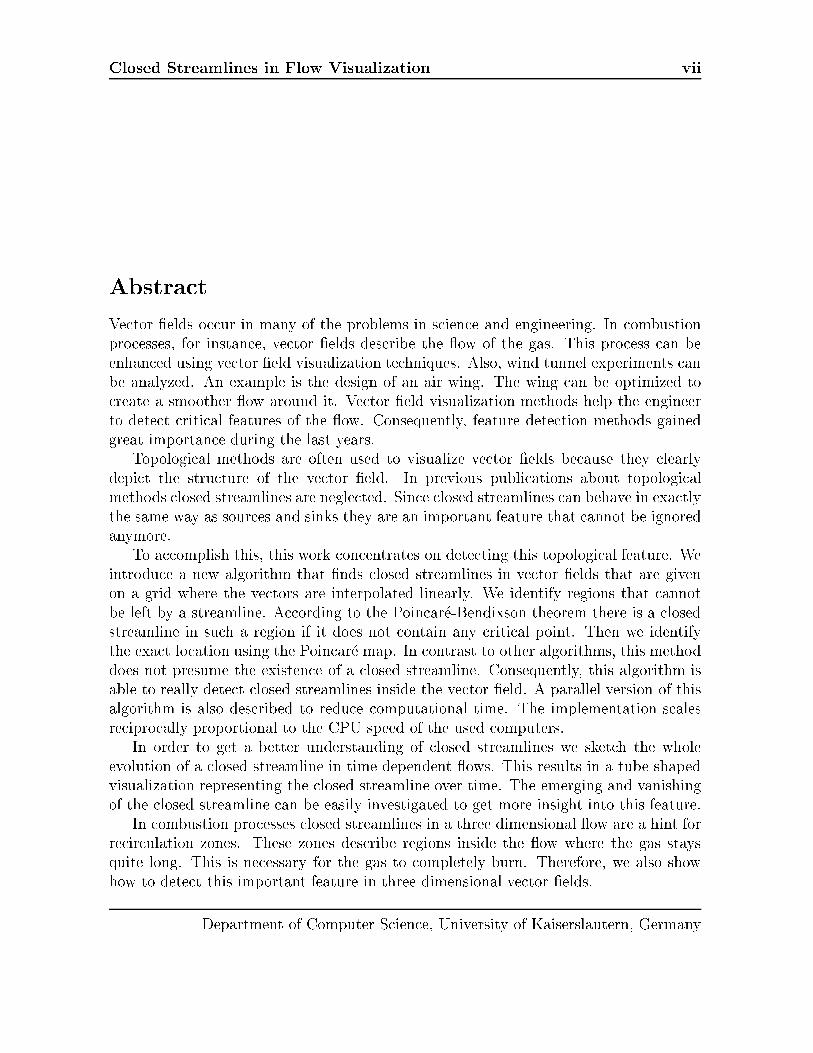
Closed Streamlines in Flow Visualization 1Chapter 1Introdu tionMany of the problems in natural s ien e and engineering involve ve tor �elds. Fluid ows, ele tri and magneti �elds are nearly everywhere, therefore measurements andsimulations of ve tor �elds are in reasing dramati ally. As with other data, analysis ismu h slower and still needs improvement. Mathemati al methods together with visu-alization an provide help in this situation. In most ases, the s ientist or engineer isinterested in integral urves of the ve tor �eld like streamlines in uid ows or mag-neti �eld lines. The qualitative nature of these urves an be studied with topologi almethods developed originally for dynami al systems. Espe ially in the area of uidme hani s, topologi al analysis and visualization have been used with su ess [GLL91℄,[HH91℄, [Ken98℄, [SHJK00℄.In visualization, topologi al methods mostly are not able to pre isely show the exis-ten e of losed streamlines. Only stopping riteria like elapsed time, number of integra-tion steps or the length of the streamline are used to prevent the algorithm from runningforever. But losed streamlines play an important role in topologi al methods be ausethey an a t in the same way as sour es or sinks; they an attra t or repel the ow.Therefore there is a strong need for an algorithm that is able to dete t this importanttopologi al feature.Figure 1.1 shows an example of a losed streamline. The streamline is started in the enter of the �gure. After a short while the integrated streamline ends up in a loop sothat the streamline y les around and around. Consequently, the omputation normallywould not terminate without dete ting this situation or using an impre ise stopping riterion like the ones mentioned before. The disadvantage with these impre ise stopping riteria is that we annot distinguish between a streamline that spirals very slowly anda streamline that runs into a losed streamline. Therefore, the streamline is stoppedto early in some ases. If we were able to really dete t whether we end up in a losedstreamline or not we an ompute the whole streamline. In this ase we additionallya elerate the integration pro ess be ause we do not y le around the losed streamlineanymore until the stopping riterion is ful�lled.Department of Computer S ien e, University of Kaiserslautern, Germany
2 Introdu tion
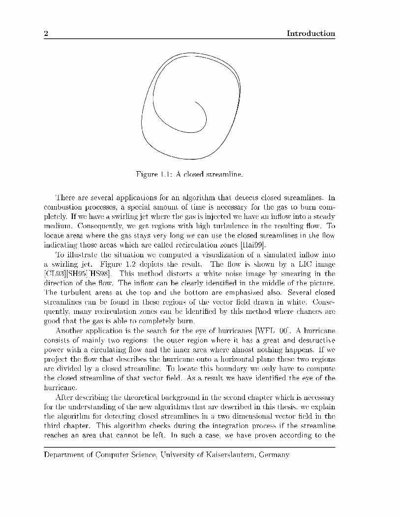
Figure 1.1: A losed streamline.There are several appli ations for an algorithm that dete ts losed streamlines. In ombustion pro esses, a spe ial amount of time is ne essary for the gas to burn om-pletely. If we have a swirling jet where the gas is inje ted we have an in ow into a steadymedium. Consequently, we get regions with high turbulen e in the resulting ow. Tolo ate areas where the gas stays very long we an use the losed streamlines in the owindi ating those areas whi h are alled re ir ulation zones [Hai99℄.To illustrate the situation we omputed a visualization of a simulated in ow intoa swirling jet. Figure 1.2 depi ts the result. The ow is shown by a LIC image[CL93℄[SH95℄[HS98℄. This method distorts a white noise image by smearing in thedire tion of the ow. The in ow an be learly identi�ed in the middle of the pi ture.The turbulent areas at the top and the bottom are emphasized also. Several losedstreamlines an be found in these regions of the ve tor �eld drawn in white. Conse-quently, many re ir ulation zones an be identi�ed by this method where han es aregood that the gas is able to ompletely burn.Another appli ation is the sear h for the eye of hurri anes [WFL+00℄. A hurri ane onsists of mainly two regions: the outer region where it has a great and destru tivepower with a ir ulating ow and the inner area where almost nothing happens. If weproje t the ow that des ribes the hurri ane onto a horizontal plane these two regionsare divided by a losed streamline. To lo ate this boundary we only have to omputethe losed streamline of that ve tor �eld. As a result we have identi�ed the eye of thehurri ane.After des ribing the theoreti al ba kground in the se ond hapter whi h is ne essaryfor the understanding of the new algorithms that are des ribed in this thesis, we explainthe algorithm for dete ting losed streamlines in a two dimensional ve tor �eld in thethird hapter. This algorithm he ks during the integration pro ess if the streamlinerea hes an area that annot be left. In su h a ase, we have proven a ording to theDepartment of Computer S ien e, University of Kaiserslautern, Germany
Closed Streamlines in Flow Visualization 3
Figure 1.2: Re ir ulation zones in a swirling jet simulation.Poin ar�e-Bendixson theorem that there exists a losed streamline in that area. To lo atethe exa t position of this losed streamline the Poin ar�e map is used.Sin e it is ne essary to ompute many streamlines to �nd every losed streamline in agiven dataset, we show a parallelization of our algorithm that dete ts losed streamlinesin hapter four. The streamlines that have to be omputed are spread as di�erent tasksto the various lients in a Linux luster. If a losed streamline is dete ted the lient sendsba k a visualization of that losed streamline to the server. The server displays all these losed streamlines. This fa ilitates a faster omputation of all losed streamlines. Thea eleration orresponds to the overall omputation power of the whole Linux luster.Inspired by the books of Abraham and Shaw [AS82℄[AS83℄[AS84℄[AS88℄ we inves-tigate the reation or vanishing of losed streamlines in hapter �ve. A ve tor �eldis interpolated over time so that losed streamlines an emerge in spe ial situations.Department of Computer S ien e, University of Kaiserslautern, Germany

4 Introdu tionThese situations are alled bifur ations. The losed streamlines are followed over time.This results in a tube shaped visualization that learly shows the evolution of the whole losed streamline.We also want to dete t losed streamlines in a three dimensional ve tor �eld. Al-though the prin iple is quite similar to the two dimensional ase there exist some essentialdi�eren es. The test if a streamline is able to leave a region is far more diÆ ult in thethree dimensional ase. This is des ribed in detail in hapter seven.
Department of Computer S ien e, University of Kaiserslautern, Germany
Closed Streamlines in Flow Visualization 5Chapter 2Theory of Ve tor FieldsThis hapter introdu es the fundamental theory whi h is needed for the following hap-ters. We mainly follow the des ription of Hirs h and Smale [HS74℄. Other des riptions an be found in [Tri02℄[GH83℄[Gu 00℄.2.1 Fundamental TheoryIn order to talk about ve tor �elds we need a pre ise de�nition of what a ve tor �elda tual is.De�nition 2.1.1 (Ve tor �eld)Let W � Rn be an open subset. An n-dimensional ve tor �eld v is de�ned as a mapv : W ! Rn :As we an see from de�nition 2.1.1 a ve tor �eld gives us an n-dimensional ve tor atan arbitrary position inside W . Ve tor �elds o ur in many appli ations. For instan e,we may have a ow in a wind tunnel experiment. This ow an be des ribed by adynami al system. If we have a massless parti le lo ated at a position x inside the ow, a dynami al system tells us where this parti le is after a given time t. Thereforea dynami al system should be ontinuously di�erentiable or at least ontinuous and ontinuously di�erentiable in t.De�nition 2.1.2 (Dynami al system)Let W � Rn be an open subset. A dynami al system or ow is a C1 map R �W �!W , where � ful�lls the following onditions:1. �(0) is the identity2. �(t) Æ �(s) = �(t+ s) for all t; s 2 RDepartment of Computer S ien e, University of Kaiserslautern, Germany
6 Theory of Ve tor FieldsWe also write �(t; x) = �t(x).There is a dire t oheren e between a dynami al system and a ve tor �eld shown bythe next remark.Remark 2.1.3Let W � Rn be an open subset and � a dynami al system. Then there exists a ve tor�eld v : W 7! Rn that satis�es v(x) = ddt�t(x)��t=0 :Thus, if x0 2 W , v(x0) is the tangent ve tor to the urve de�ned by t ! �t(x0) att = 0. From another point of view we an start with a given ve tor �eld v. With a givenpoint x0 2 W , this leads us to the Cau hy problem.De�nition 2.1.4 (Cau hy problem)Let v be a ve tor �eld as in de�nition 2.1.1 and x0 2 W an arbitrary point. Then theCau hy problem is de�ned by the di�erential equationddtx(t) = v(x(t))with the so alled initial ondition x(0) = x0.Then the dynami al system � satisfying the equation in remark 2.1.3 gives us thesolution urve x(t) = �t(x) for the Cau hy problem.Remark 2.1.5The solution urve is also referred to as a streamline, an integral urve, a traje -tory, or an orbit.v(x )
x(t)x = x(t )0
0
0
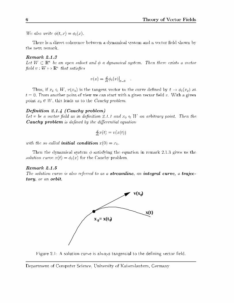
Figure 2.1: A solution urve is always tangential to the de�ning ve tor �eld.Department of Computer S ien e, University of Kaiserslautern, Germany
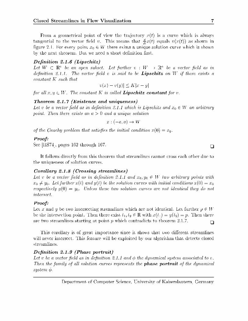
Closed Streamlines in Flow Visualization 7From a geometri al point of view the traje tory x(t) is a urve whi h is alwaystangential to the ve tor �eld v. This means that ddtx(t) equals v(x(t)) as shown in�gure 2.1. For every point x0 2 W there exists a unique solution urve whi h is shownby the next theorem. But we need a short de�nition �rst.De�nition 2.1.6 (Lips hitz)Let W � Rn be an open subset. Let further v : W ! Rn be a ve tor �eld as inde�nition 2.1.1. The ve tor �eld v is said to be Lips hitz on W if there exists a onstant K su h that jv(x)� v(y)j � Kjx� yjfor all x; y 2 W . The onstant K is alled Lips hitz onstant for v.Theorem 2.1.7 (Existen e and uniqueness)Let v be a ve tor �eld as in de�nition 2.1.1 whi h is Lips hitz and x0 2 W an arbitrarypoint. Then there exists an a > 0 and a unique solutionx : (�a; a)! Wof the Cau hy problem that satis�es the initial ondition x(0) = x0.Proof:See [HS74℄, pages 162 through 167. ❏It follows dire tly from this theorem that streamlines annot ross ea h other due tothe uniqueness of solution urves.Corollary 2.1.8 (Crossing streamlines)Let v be a ve tor �eld as in de�nition 2.1.1 and x0; y0 2 W two arbitrary points withx0 6= y0. Let further x(t) and y(t) be the solution urves with initial onditions x(0) = x0respe tively y(0) = y0. Unless these two solution urves are not identi al they do notinterse t.Proof:Let x and y be two interse ting streamlines whi h are not identi al. Let further p 2 Wbe the interse tion point. Then there exist t1; t2 2 R with x(t1) = y(t2) = p. Then thereare two streamlines starting at point p whi h ontradi ts to theorem 2.1.7. ❏This orollary is of great importan e sin e it shows that two di�erent streamlineswill never interse t. This feature will be exploited by our algorithm that dete ts losedstreamlines.De�nition 2.1.9 (Phase portrait)Let v be a ve tor �eld as in de�nition 2.1.1 and � the dynami al system asso iated to v.Then the family of all solution urves represents the phase portrait of the dynami alsystem �. Department of Computer S ien e, University of Kaiserslautern, Germany

8 Theory of Ve tor FieldsIt is also possible to investigate ve tor �elds over time. Therefore we de�ne timedependent ve tor �elds.De�nition 2.1.10 (Time dependent ve tor �eld)Let W � Rn be an open subset. An n-dimensional time dependent ve tor �eld vis de�ned as a map v : R �W ! Rn(t; x) 7! v(x)where t is the time parameter.2.2 Data Stru turesIn most appli ations in S ienti� Visualization the data is not given as a losed formsolution. The same holds for ve tor �elds. Usually, the ve tor �elds result from asimulation or an experiment where the ve tors are measured. In su h a ase, the ve torsare given at only some points of the domain of the Eu lidean spa e. These points arethen onne ted by a grid. A spe ial interpolation omputes the ve tors inside ea h ellof the grid. In this hapter we restri t ourselves to the few types of grids that we usedin our algorithms in this se tion.2.2.1 Triangular Grids
Figure 2.2: Triangular grid.A very popular two dimensional grid type is the triangular grid. Figure 2.2 showsan example for su h a grid. This grid type fa ilitates to onne t an arbitrary point set.To get the ve tors inside a ell we use an interpolation s heme based on bary entri Department of Computer S ien e, University of Kaiserslautern, Germany

Closed Streamlines in Flow Visualization 9p
p
p
b
b1−b
b
2
1
0
0
1 2
1−b
p1−b21
0
Figure 2.3: Bary entri oordinates. oordinates. Figure 2.3 explains the on�guration. Let p be the point where we wantto interpolate the ve tor and p0, p1, and p2 are the verti es of the triangle.The bary entri oordinates b0, b1, and b2 des ribe the distan es between the pointpi and the edge whi h is opposite to the vertex with the same index. For the bary entri oordinates the equation P2i=0 bi = 1 holds. The point p an be expressed in thefollowing way: p = 2Xi=0 bi � pi :Let v(pi) be the ve tors at the verti es of the triangle. Then we an interpolate theve tor v(p) at the point p in the same way:v(p) = 2Xi=0 bi � v(pi) :To ompute the zeros inside the triangle we need to solve the following linear equa-tion: 2Xi=0 bi � v(pi) = 0 :Unless this system is degenerated, the solution is unique. Consequently, we get at mostone zero depending on whether the solution point lies inside the triangle or not.Department of Computer S ien e, University of Kaiserslautern, Germany

10 Theory of Ve tor Fields2.2.2 Quadrilateral Grids
(a) Re tilinear grid. (b) Curvilinear grid.Figure 2.4: Quadrilateral grids.There exist two di�erent types of quadrilateral grids. The �rst one is the re tilineargrid. There every ell is a re tangle. The edges of the ells are orthogonal as shownin �gure 2.4a. The other type is the urvilinear grid. Here the boundary between the ells is a urve onsisting of points onne ted by straight lines. The boundary of morethan one ell does not need to be a straight line anymore as an be seen in �gure 2.4b.If we interpolate in su h a ell we need to map it to a re tangular ell. This map � isnot linear. Often one speaks of mapping from physi al spa e into omputational spa e.Usually, a numeri al method is used to do this mapping. Consequently, we an restri tourselves to the re tangular ase when explaining interpolation in this ase.p
pp
p
ps
r
2
0 1
3
Figure 2.5: Lo al oordinates inside a re tangle.We interpolate bilinearly inside ea h ell. Therefore, we introdu e lo al oordinates(r; s) with 0 � s; r � 1 inside the ell of the point p where we want to interpolate.Department of Computer S ien e, University of Kaiserslautern, Germany

Closed Streamlines in Flow Visualization 11Figure 2.5 explains how this works. The vertex p0 has lo al oordinates (0; 0), thevertex p1 the oordinates (1; 0), the vertex p2 orresponds to (1; 1), while the last vertexp3 is lo ated at (0; 1). Then we an use the following formula for the interpolation:v(p) = (1� r)(1� s) � v(p0) + r(1� s) � v(p1) + rs � v(p2) + (1� r)s � v(p3) :2.2.3 Tetrahedral Grids
Figure 2.6: Tetrahedron.A tetrahedral grid onsists of several tetrahedrons as shown in �gure 2.6. Conse-quently, a tetrahedral grid is a three dimensional grid. As with triangular grids anarbitrary point set an be onne ted using this grid type. The interpolation s hemeworks in an analogue way as the triangular ase using bary entri oordinates. Con-sequently, there is at most one zero inside ea h tetrahedron, also, if the interpolatingve tor �eld is non-degenerate inside that tetrahedron.2.2.4 Time dependent Data with Prism CellsWhen dealing with time-dependent two-dimensional ows we an use the third dimen-sion to represent time. We assume the ve tor �eld is given at time sli es on a triangulargrid. These time sli es vi : W ! R2 are onne ted using prism ells as shown in�gure 2.7. To interpolate the ve tors we onsider the following mapf : R �W �! R � R2(t; x) 7! v(t; x)where W is the domain represented by the two dimensional grid of the time sli es. Sin ewe need onsisten y with the pie ewise aÆne linear interpolation that would be appliedon a 2D triangulation, we have to ensure that the restri tion of the 3D interpolantto ea h time plane is pie ewise aÆne linear, too. That means that, �xing the timeDepartment of Computer S ien e, University of Kaiserslautern, Germany

12 Theory of Ve tor Fields����
����������������������������������������������������������������������������������������������������������������������������������������
��������������������������������
��������������������������������
��������������������������������������������������������������������������������������������������
��������������������������������
���������������������
���������������������
t = t i+1t = t i
T
Figure 2.7: Time prism ell. oordinate and taking it as a parameter, the interpolant must be aÆne linear. This isthe reason why we hoose the following interpolant inside ea h prism ell.For a given prism ell lying between ti and ti+1, let vj(x) = Ajx + bj, j 2 fi; i + 1gbe the linear interpolation orresponding to the prism triangle fa es lying in the planesft = tig and ft = ti+1g respe tively. Then we de�ne the interpolant over the wholeprism ell by linear interpolation over time:v(t; x) = ti+1 � tti+1 � ti vi(x) + t� titi+1 � tivi+1(x)where t 2 [ti; ti+1℄. This formula obviously ensures, for ea h �xed value of t, that v(x; t)is aÆne linear in x.2.3 Criti al PointsCriti al points are from a topologi al point of view an important part of ve tor �elds.This spe ial feature is des ribed in more detail in this se tion. We �rst explain thegeneral ase and then study the linear ase.2.3.1 General CaseWe start with the de�nition of riti al points in the general ase. Then we lassifydi�erent types of singularities and talk about stability whi h is ne essary to a hieve aDepartment of Computer S ien e, University of Kaiserslautern, Germany

Closed Streamlines in Flow Visualization 13meaningful physi al interpretation of ve tor �elds.De�nition 2.3.1 (Criti al point)Let v : W ! Rn be a ve tor �eld as in de�nition 2.1.1 whi h is ontinuously di�eren-tiable. Let further x0 2 W be a point where v(x) = 0. Then x0 is alled a riti alpoint of the ve tor �eld.Remark 2.3.2There are several di�erent terms for riti al points. They are also known as singular-ities, singular points, zeros, or equilibriums.2.3.1.1 Classi� ationCriti al points an be lassi�ed using the eigenvalues of the derivation of the ve tor�eld. For instan e, we an identify sinks that purely attra t the ow in the vi initywhile sour es repel it purely.De�nition 2.3.3 (Sink)Let v be a ve tor �eld as in de�nition 2.1.1 whi h is ontinuously di�erentiable and x0a riti al point of v. Let further Dv(x0) be the derivation of the ve tor �eld v at x0. Ifall eigenvalues of Dv(x0) have negative real parts, x0 is alled a sink.The following theorem shows that sinks really have an attra ting property.Theorem 2.3.4Let v : W ! Rn be a ve tor �eld and x0 a sink. Let further � be the orrespondingdynami al system. Let us assume the real part of every eigenvalue is less than � , > 0. Then there exists a neighborhood U � W of x0 su h that1. �t(x) 2 U for all x 2 U , t > 0.2. There is an Eu lidean norm on Rn su h thatj�t(x)� x0j � e�t jx� x0jfor all x 2 U , t � 0.3. For any norm on Rn , there is a onstant B > 0 su h thatj�t(x)� x0j � Be�t jx� x0jfor all x 2 U , t � 0.Proof:See [HS74℄, pages 181 and 182. ❏Department of Computer S ien e, University of Kaiserslautern, Germany

14 Theory of Ve tor FieldsCorollary 2.3.5Let v, �, and xo be as in the previous theorem. Then there exists a neighborhood U � Wof x0 so that �t(x) onverges to x0:�t(x)! x0 as t!1 for all x 2 UIn the same way we an de�ne sour es.De�nition 2.3.6 (Sour e)Let v be a ve tor �eld as in de�nition 2.1.1 whi h is ontinuously di�erentiable and x0a riti al point of v. Let further Dv(x0) be the derivation of the ve tor �eld v at x0. Ifall eigenvalues of Dv(x0) have positive real parts, x0 is alled a sour e.2.3.1.2 StabilitySin e in omputer s ien e absolute exa t al ulation is not possible due to numeri alerrors we need some sort of stability if we really want to lassify riti al points algorith-mi ally. A riti al point that hanges its behavior even when the ve tor �eld is slightlyperturbed does not have a very signi� ant meaning in a physi al sense.U
1U
x 0
Figure 2.8: A riti al point that is stable.De�nition 2.3.7 (Stable riti al point)Let v : W ! Rn be a ve tor �eld as in de�nition 2.1.1 whi h is ontinuously di�erentiableand x0 a stable riti al point of v. If for every neighborhood U � W of x0 there is aneighborhood U1 � U of x0 su h that every streamline x(t) with x(0) 2 U1 is de�ned andx(t) 2 U for all t > 0 then x0 is alled a stable riti al point.Figure 2.8 illustrates a stable on�guration.Department of Computer S ien e, University of Kaiserslautern, Germany

Closed Streamlines in Flow Visualization 15U
1U
x 0
Figure 2.9: An asymptoti ally stable riti al point.De�nition 2.3.8 (Asymptoti ally stable riti al point)Let v, U , and U1 be as in the previous de�nition. If in addition U1 an be hosen sothat limt!1 x(t) = x0 then x0 is alled an asymptoti ally stable riti al point.In �gure 2.9 we sket h this situation.U
x 0
Figure 2.10: A riti al point that is unstable.De�nition 2.3.9 (Unstable riti al point)Let v :W ! Rn be a ve tor �eld as in de�nition 2.1.1 whi h is ontinuously di�erentiableand x0 a stable riti al point of v. We all a riti al point that is not stable an unstable riti al point. This means that there is a neighborhood U � W of x0 su h that for everyDepartment of Computer S ien e, University of Kaiserslautern, Germany

16 Theory of Ve tor Fieldsneighborhood U1 � U of x0 there is at least one streamline x(t) starting at x(0) 2 U1whi h does not ompletely lie in U .Figure 2.10 shows an unstable riti al point.Figure 2.11: A riti al point that is stable but not asymptoti ally stable.For example, a sink is an asymptoti ally stable riti al point and therefore stable.An example of a riti al point that is stable but not asymptoti ally stable is shown in�gure 2.11. All streamlines surround the riti al point ellipti ally. This on�gurationis rather riti al be ause the slightest perturbation will hange the riti al point into asour e or a sink. Therefore, we want to distinguish between su h numeri ally riti alsituations and numeri ally stable ones.Theorem 2.3.10Let v be a ve tor �eld as in de�nition 2.1.1 whi h is ontinuously di�erentiable and x0a stable riti al point of v. Then no eigenvalue of Dv(x0) has positive real part.Proof:See [HS74℄, pages 187 and 188. ❏To have a ommon term for su h numeri ally stable on�gurations we use the notionof hyperboli ity.De�nition 2.3.11 (Hyperboli riti al point)Let v be a ve tor �eld as in de�nition 2.1.1 whi h is ontinuously di�erentiable and x0a riti al point of v. If the derivative Dv(x0) has no eigenvalue with real part zero the riti al point is alled hyperboli .Corollary 2.3.12A hyperboli riti al point is either unstable or asymptoti ally stable.This orollary shows that hyperboli riti al points avoid numeri ally riti al situa-tions. These points an be dete ted algorithmi ally sin e the behavior does not signi�- antly hange if there is a numeri al error that is small enough.Department of Computer S ien e, University of Kaiserslautern, Germany

Closed Streamlines in Flow Visualization 172.3.2 Linear CaseSin e we use linear or bilinear interpolation in our algorithms we want to analyze thelinear ase in more detail. This also gives a better insight into the di�erent types of riti al points. Therefore we examine riti al points in linear ve tor �elds. First of all,we need to de�ne what we exa tly mean by a linear ve tor �eld.De�nition 2.3.13 (Linear ve tor �eld)Let W � Rn be an open subset. A ve tor �eldv : W ! Rnis alled linear, if there exists a linear mapA : W ! Rnand a ve tor b 2 Rn su h that v(x) = Ax+ b 8x 2 Wif in addition b = 0 then v is alled homogeneous linear.To get a better insight into linear ve tor �elds we investigate the phase portrait ofthe di�erent types of linear ve tor �elds. If we restri t ourselves to the hyperboli asewhere detA 6= 0 the ve tor b only gives a displa ement so that we an negle t it in our onsideration. Nielson [NJ99℄ summarized all di�erent ases that are possible. A linearve tor �eld an have at most one riti al point due to the linearity. In order to get thephase portrait we have to solve the Cau hy problemddtx(t) = Axwith initial ondition x(0) = k, k 2 Rn .Lemma 2.3.14Let v be a homogeneous linear ve tor �eld, whi h is des ribed by the matrix A 2Mat(n�n). Then there exists a solution for the di�erential equationddtx(t) = Ax(t) with initial ondition x(0) = k 2 Rn (2.1)whi h is given by: x = etAk with eA = 1Xk=0 Akk! (2.2)Department of Computer S ien e, University of Kaiserslautern, Germany

18 Theory of Ve tor FieldsProof:Compute the derivation ddtx(t):ddtetAk = k � ddtetA = k � AetAsin e the derivation of etA an be omputed as follows:ddtetA = limh!0 e(t+h)A � etAh= limh!0 etAehA � etAh= etA limh!0 ehA � Ih= etA � A❏Let us have a loser look at two dimensional linear ve tor �elds whi h an be de-s ribed by a matrix A 2 Mat(2 � 2). Then, we an distinguish between di�erent aseswhere we are able to ompute the derivation.Lemma 2.3.15Let A 2 Mat(2 � 2) be a two dimensional matrix. Then there is an invertible matrixP su h that B = PAP�1, where B orresponds to one of the following three di�erenttypes. �; � 2 C are the eigenvalues of A.Type one: A is diagonalizable: B = �� 00 ��Type two: � and � have non zero imaginary part:B = �a �bb a �Type three: � = � and A is not diagonalizable:B = �� 01 ��The next subse tions des ribe the di�erent types in detail. The di�erential equationis solved to sket h the phase portrait. We assume that the matri es of the ve tor �eldsare given in the form as shown in lemma 2.3.15.Department of Computer S ien e, University of Kaiserslautern, Germany
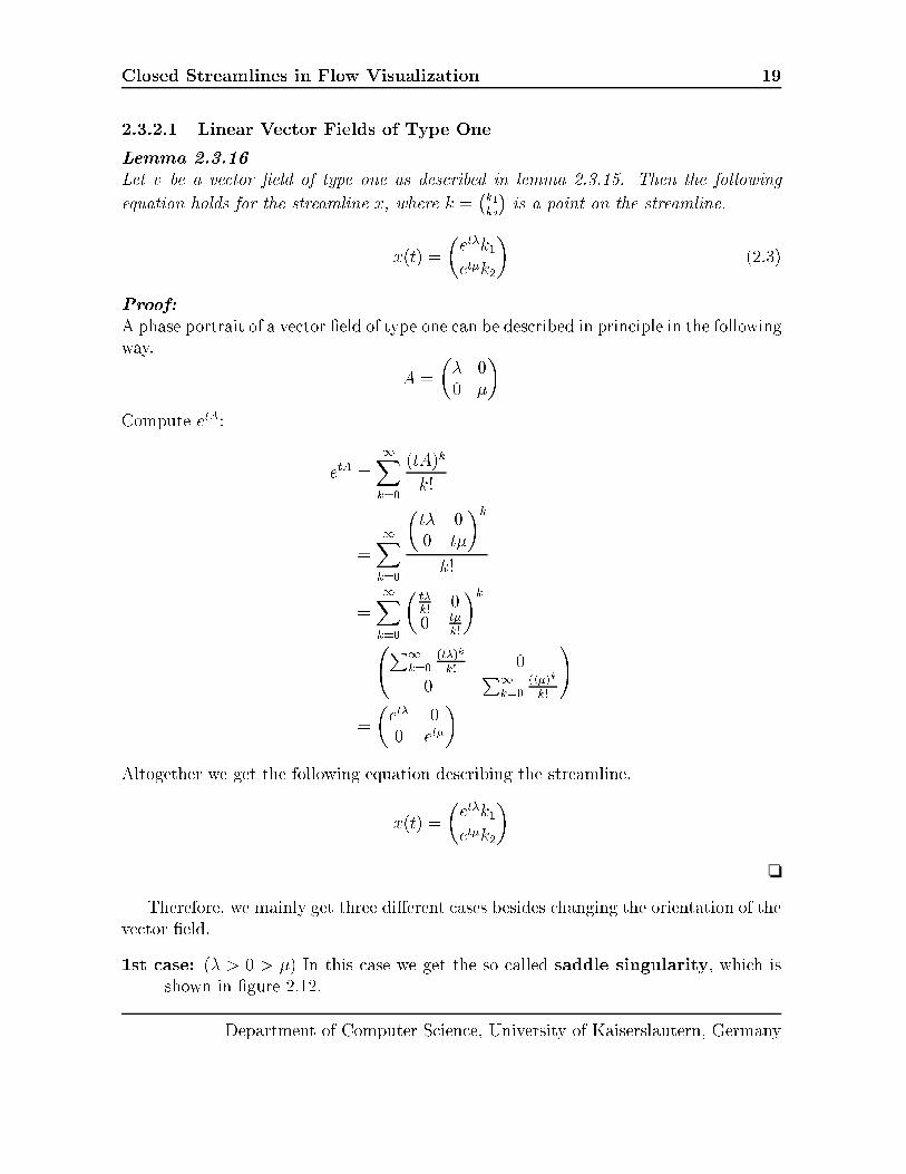
Closed Streamlines in Flow Visualization 192.3.2.1 Linear Ve tor Fields of Type OneLemma 2.3.16Let v be a ve tor �eld of type one as des ribed in lemma 2.3.15. Then the followingequation holds for the streamline x, where k = �k1k2� is a point on the streamline.x(t) = �et�k1et�k2� (2.3)Proof:A phase portrait of a ve tor �eld of type one an be des ribed in prin iple in the followingway. A = �� 00 ��Compute etA: etA = 1Xk=0 (tA)kk!= 1Xk=0 �t� 00 t��kk!= 1Xk=0 � t�k! 00 t�k!�k= P1k=0 (t�)kk! 00 P1k=0 (t�)kk! != �et� 00 et��Altogether we get the following equation des ribing the streamline.x(t) = �et�k1et�k2�❏Therefore, we mainly get three di�erent ases besides hanging the orientation of theve tor �eld.1st ase: (� > 0 > �) In this ase we get the so alled saddle singularity, whi h isshown in �gure 2.12.Department of Computer S ien e, University of Kaiserslautern, Germany

20 Theory of Ve tor Fields
Figure 2.12: A saddle singularity.
Figure 2.13: A node singularity.2nd ase: (� < � < 0) An example for this ase is the so alled node singularityshown in �gure 2.13.3rd ase: (� = � < 0) Figure 2.14 shows su h a fo us singularity.2.3.2.2 Linear Ve tor Fields of Type TwoThe matrix A that represents the ve tor �eld mathemati ally des ribes a rotation anda s aling. This an be shown easily when we de�ne a rotational angle � := ar os(ar )where we set r := pa2 + b2. We an dedu e that:a = r os� (2.4)b = r sin� (2.5)Then we an write the matrix A as follows:A = �r 00 r� � � os� � sin�sin� os� � (2.6)Department of Computer S ien e, University of Kaiserslautern, Germany

Closed Streamlines in Flow Visualization 21
Figure 2.14: A fo us singularity.Lemma 2.3.17Let v be a ve tor �eld of type two. Then the following equation des ribes a streamlinewhere k = �k1k2� is a point on the streamline.x(t) = eta � �k1 os(tb)� k2sin(tb)k1sin(tb) + k2 os(tb)� (2.7)Proof:We interpret the map T given by the matrix A algebrai ally by identifying R2 with the omplex spa e C . (x; y)$ x+ iy (2.8)We get the following orresponden e for T :(x; y) ! x+ iyx?yT x?yMultiplying with a+ib(ax� by; bx + ay) ! (ax� by) + i(bx + ay) (2.9)In the same way there is a orresponden e eA $ ea+b. This results with eA = �a1 a2a3 a4�in the following s heme:(x; y) ! x+ iyx?yeA x?yea+ib(a1x+ a2y; a3x + a4y) ! ea(x os b� y sin b+ i(x sin b + y os b)) (2.10)By omparing the oeÆ ients we an on lude that the matrix eA an be representedas follows: eA = ea � � os b � sin bsin b os b �Department of Computer S ien e, University of Kaiserslautern, Germany

22 Theory of Ve tor FieldsA ording to lemma 2.3.14 the following equation holds for a streamline ontaining thepoint k = �k1k2�. x(t) = eta ��k1 os(tb)� k2sin(tb)k1sin(tb) + k2 os(tb)� (2.11)❏
Figure 2.15: A enter singularity.
Figure 2.16: A spiral singularity.With this equation we an see how the streamlines behave in su h a ve tor �eld. Ifwe have a = 0, the ve tor �eld des ribes simple ir les as shown in �gure 2.15, while weget a spiral shaped phase portrait if we set a 6= 0 as sket hed in �gure 2.16.Department of Computer S ien e, University of Kaiserslautern, Germany

Closed Streamlines in Flow Visualization 232.3.2.3 Linear Ve tor Fields of Type ThreeLemma 2.3.18Let v be a ve tor �eld of type three and A the orresponding matrix where v(x) = Axand A = �� 01 ��. Then we an des ribe a streamline ontaining the point k = �k1k2� withthe following equation: x(t) = et� � � k1k1t + k2� (2.12)Proof:The matrix A an be split up in the following way:A = �� 01 �� = � � I + �0 01 0�For the matrixM = �0 01 0� the following equation holds whi h an be easily omputed.M2 = �0 00 0� = 0Consequently, we get Mk = 0 for all k � 2.Then we an ompute etA as follows:etA = et(�I+M)= et�I+0�0 0t 01A= et�I � e0�0 0t 01A= et�I � (I + �0 0t 0�) , using the above equation= et� � �1 0t 1�Therefore, the following equation des ribes a streamline ontaining the point k = �k1k2�.x(t) = et� � � k1k1t + k2� (2.13)❏Figure 2.17 shows an example for su h an improper node singularity.Department of Computer S ien e, University of Kaiserslautern, Germany

24 Theory of Ve tor Fields
Figure 2.17: An improper node singularity.2.4 Streamline ComputationIn this se tion we des ribe the omputation of streamlines. Sin e the ve tor �eld isgiven on a triangular, quadrilateral, or tetrahedral grid the ve tors inside the ells areinterpolated linearly respe tively bilinearly. In order to ompute a streamline we haveto solve the Cau hy problem where the initial ondition is given by the starting pointof the streamline. Therefore we need to solve a di�erential equation. Consequently, thestreamlines itself have to be al ulated using ODE solvers like for instan e Runge-Kutta.The streamlines an be integrated in positive or negative dire tion starting at the givenstarting point. To integrate in negative dire tion we only need to invert the ve tor �eld.In addition, it is possible to ompute streamlines exa tly inside triangular ells.2.4.1 Numeri al ComputationFor numeri al integration we use standard methods that an be found in the numeri alliterature [Tri02℄[Feh69℄[PTVF92℄[Gu 00℄. We favor predi tor- orre tor methods likeRunge-Kutta method with adaptive stepsize. An optimized implementation for a �fthorder Runge-Kutta method with adaptive stepsize an be found in [PTVF92℄. Thesemethods only use the interpolation method inside the ells but do not depend on aspe ial type of grid.2.4.2 Exa t ComputationOn a triangular grid the ve tor �eld is interpolated linearly. Inside a triangular ell we an represent the ve tor �eld as a single linear ve tor �eld as in subse tion 2.3.2. Inthis subse tion we also explained an exa t solution of the di�erential equation that hasto be solved in order to ompute a streamline. This method was �rst introdu ed byNielson [NHM97℄. Consequently, we an al ulate a streamline starting at an arbitraryDepartment of Computer S ien e, University of Kaiserslautern, Germany

Closed Streamlines in Flow Visualization 25starting point using these formulas inside a triangle. When the streamline leaves thetriangle we determine the interse tion with one of the edges of the triangle numeri ally.Then we an start the integration pro ess in the neighboring ell at that interse tion.This way we an go from one triangle to another.2.5 Closed StreamlinesWhen omputing streamlines it often happens that the streamline omputation doesnot terminate. This is mostly due to losed streamlines where the streamline ends upin a loop that annot be left. These losed streamlines are introdu ed and explainedin this se tion. More about the theoreti al ba kground an be found in several books[YqSlLs+86℄[Rou98℄.2.5.1 Limit SetsThe topologi al analysis of ve tor �elds onsiders the asymptoti behavior of streamlines.There we have two di�erent kind of so alled limit sets, the origin set or �-limit set ofa streamline and the end set or !-limit set.De�nition 2.5.1 (�-limit set)Let s be a streamline in a given ve tor �eld v. Then we de�ne the �-limit set as thefollowing set: fp 2 R2 j9(tn)1n=0 � R; tn ! �1; limn!1 s(tn)! pgDe�nition 2.5.2 (!-limit set)Let s be a streamline in a given ve tor �eld v. Then we de�ne the !-limit set as thefollowing set: fp 2 R2 j9(tn)1n=0 � R; tn !1; limn!1 s(tn)! pgRemark 2.5.3Let v be a ve tor �eld as in de�nition 2.1.1. We speak of an �- or !-limit set L of v ifthere exists a streamline s in the ve tor �eld v that has L as �- or !-limit set.If the �- or !-limit set of a streamline onsists of only one point, this point is a riti alpoint. The most ommon ase of a �- or !-limit set in a planar ve tor �eld ontainingmore than one inner point of the domain is a losed streamline whi h is de lared in thenext de�nition. Figure 2.18 shows an example for �- and !-limit sets. Here we have a riti al point and a losed streamline. The riti al point and the losed streamline aretheir own �- and !-limit set. For every other streamline the losed streamline is the!-limit set. If the streamline starts inside the losed streamline the riti al point is theDepartment of Computer S ien e, University of Kaiserslautern, Germany

26 Theory of Ve tor Fields����
Figure 2.18: Example for �- and !-limit sets.�-limit set. Otherwise the �-limit set is empty. Now that we showed an example for a losed streamline let us give a pre ise de�nition.De�nition 2.5.4 (Closed streamline)Let v be a ve tor �eld as in de�nition 2.1.1. A losed streamline : R ! Rn ; t 7! (t)is a streamline of a ve tor �eld v su h that there is a t0 2 R with (t+ nt0) = (t) 8n 2 Nand not onstant.Remark 2.5.5There are several di�erent terms des ribing a losed streamline. The terms limit y le, losed orbit, and losed streamline are equivalent.Similar to riti al points we de�ne asymptoti ally stability of losed streamlines. Ifa losed streamline is asymptoti ally stable it is attra ting.De�nition 2.5.6 (Asymptoti ally stability of losed streamlines)Let v : W ! Rn be a ve tor �eld as in de�nition 2.1.1 that is ontinuously di�erentiable.Let further � be the orresponding dynami al system and � W a losed streamline. Iffor every neighborhood U � W with � U there is a neighborhood U1 � U with � U1su h that �t(x) 2 U for all x 2 U1 and t > 0 andlimt!1minfk�t(x)� zkjz 2 g = 0then is alled asymptoti ally stable losed streamline.This means that an asymptoti ally stable losed streamline attra ts the ow inside aspe ial neighborhood. It also follows from this de�nition that an asymptoti ally stable losed streamline is isolated from other losed orbits. In the same way there are losedstreamlines that are repelling. For instan e, by inverting the ve tor �eld we an turnan attra ting losed streamline into a repelling one.Department of Computer S ien e, University of Kaiserslautern, Germany

Closed Streamlines in Flow Visualization 272.5.2 Poin ar�e Map
y
R(y)
x
S
R(x)
(a) x
P
P
R(x)R
S
S(b)Figure 2.19: Poin ar�e se tion (a) and Poin ar�e map (b).Let us assume we have a two dimensional ve tor �eld ontaining one limit y le.Then we an hoose a point P on the limit y le and draw a ross se tion S whi h isa line segment not parallel to the limit y le a ross the ve tor �eld. This line is alleda Poin ar�e se tion. If we start a streamline at an arbitrary point x on S and followit until we ross the Poin ar�e se tion S again, we get another point R(x) on S. Thisresults in the Poin ar�e map R. Figure 2.19 illustrates the situation. The left part showsthe Poin ar�e se tion with the limit y le in the middle drawn with a thi ker line, whilethe right part displays the Poin ar�e map itself. Obviously the point P on the limit y leis mapped onto itself. Consequently, it is a �xed point of the Poin ar�e map.Let us pre ise this in some de�nitions:De�nition 2.5.7 (Cross se tion)Let v be a ve tor �eld as in de�nition 2.1.1 and S � Rn an open set on a hyperplaneof dimension n� 1 that is transverse to v. Transverse to v means that v(x) =2 S for allx 2 S. Then S is alled a ross se tion.De�nition 2.5.8 (Poin ar�e map)Let v be a ve tor �eld and � the dynami al system belonging to v. Let further be S a ross se tion that interse ts a losed streamline at a point P . Then the Poin ar�e mapis de�ned as the map R : S ! S su h thatx 7! �t(x) ;Department of Computer S ien e, University of Kaiserslautern, Germany

28 Theory of Ve tor Fieldswhere t is the time the streamline started at x needs to interse t the ross se tion againafter one turn.Remark 2.5.9It is obvious that the point P on the losed streamline is a �xed point of the Poin ar�emap.2.5.3 The Poin ar�e-Bendixson TheoremIn this subse tion we show a fundamental result whi h makes it easier to �nd losedstreamlines in a two dimensional ve tor �eld. This property is exploited by our algorithmwhi h is introdu ed later.Theorem 2.5.10 (Poin ar�e-Bendixson Theorem)Let W � R2 be an open subset and v : W ! R2 a two dimensional, ontinuouslydi�erentiable ve tor �eld. Let further L � W be a nonempty ompa t limit set of theve tor �eld v that ontains no riti al point. Then L des ribes a losed streamline.Proof:See [HS74℄, pages 248 and 249. ❏Corollary 2.5.11Let W � R2 be an open subset and v : W ! R2 a two dimensional, ontinuouslydi�erentiable ve tor �eld. Let further D � W be a nonempty ompa t subset whi h ontains no riti al point and s a streamline inside D. If the streamline s does not leaveD then there exists a losed streamline inside D.Using this orollary our algorithm to dete t losed streamlines an simply integratea streamline and he k during the integration pro ess if it runs into a ompa t regionthat is never left. If we �nd su h a region this orollary states that we found a losedstreamline.2.6 Ve tor Field TopologyThe topologi al graph, or simply topology, of a ve tor �eld des ribes the stru ture ofthe phase portrait. Considering saddle singularities we an de�ne separatri es.De�nition 2.6.1 (Separatri es)Let v be a ve tor �eld as in de�nition 2.1.1 and x0 a saddle singularity. The streamlinesemerging in eigendire tion are alled separatri es.Department of Computer S ien e, University of Kaiserslautern, Germany

Closed Streamlines in Flow Visualization 29Ea h separatrix onne ts the saddle point with another riti al point or the boundaryof the ve tor �eld. The separatri es divide the ve tor �eld in various topologi al regions.Ea h region annot be left by an individual streamline ex ept for the ase where thestreamline rosses the boundary. Furthermore, every streamline in that region thatdoes not rea h the boundary onverges to the same riti al point or losed streamlinefor t ! 1 and to the same riti al point or losed streamline for t ! �1. Now weintrodu ed every on ept needed for ve tor �eld topology.De�nition 2.6.2 (Topology)Let v be a ve tor �eld as in de�nition 2.1.1. The topology is built by all riti al points,separatri es and losed streamlines of v.
(a) (b)Figure 2.20: Topologi al graphs of two ve tor �elds.Figure 2.20 shows two examples for topologi al graphs of a simple ve tor �eld. The riti al points are olored a ording to its type: saddles are drawn in red, sinks are bluewhile sour es are olored green. The ve tor �eld in sub�gure (a) ontains one losedstreamline while the other sub�gure does not ontain any losed streamlines. In bothpi tures we an learly re ognize the prin iple stru ture of the ow inside the ve tor�elds. Department of Computer S ien e, University of Kaiserslautern, Germany

30 Theory of Ve tor Fields2.7 Stru tural StabilityIf a ve tor �eld is slightly perturbed it may happen that the topology stays the same if the hange is suÆ iently small. This means that there exists a homeomorphism that mapsea h streamline of the original ow to the perturbed one. This homeomorphism gives aone-to-one orresponden e between riti al points and losed streamlines of the ow. Ifsu h a homeomorphism exists we say that the two ows are topologi ally equivalent.De�nition 2.7.1 (Topologi ally equivalent)Let v and w be two ve tor �elds as in de�nition 2.1.1. Let further � and be thedynami al system a ording to v respe tively w. If there exists a homeomorphism h :Rn ! Rn su h that for any t1 there is a t2 withh(�t1(x)) = t2(x)then v and w are topologi ally equivalent.To de�ne neighboring ve tor �elds we need a norm on ve tor �elds �rst. Then we an de�ne neighboring ve tor �elds as ve tor �elds that di�er only slightly.De�nition 2.7.2Let v be ve tor �eld as in de�nition 2.1.1 that is ontinuous di�erentiable. Then thenorm kvk of a ve tor �eld is de�ned as kvk = max(fkv(x)kjx 2 Wg [ fkDv(x)kjx 2Wg). We allow kvk =1.De�nition 2.7.3 (Neighborhood)Let v be a ve tor �eld as in de�nition 2.1.1 that is ontinuous di�erentiable. Let furtherN = fw 2 fvjv : W ! Rngjkv � wk < �g. This means that every ve tor �eld w 2 N isa perturbed version of v. Then N is alled a neighborhood of v.If there exists a neighborhood N of a given ve tor �eld v where every ve tor �eld istopologi ally equivalent to the other, the ve tor �eld v is alled stru tural stable. Thismeans that the topology of the ve tor �eld that is slightly perturbed stays the same.The following de�nition pre ises that.De�nition 2.7.4 (Stru tural stable)Let v be a ve tor �eld as in de�nition 2.1.1. If there is a neighborhood N of v su hthat every ve tor �eld w 2 N is topologi ally equivalent to v then v is alled stru turalstable.We now want to give a theorem that explains when a two dimensional ve tor �eldis stru tural stable. But �rst we need a de�nition whi h shows a spe ial on�guration on erning saddle singularities. Ve tor �elds ontaining su h a on�guration an neverbe stru tural stable.Department of Computer S ien e, University of Kaiserslautern, Germany

Closed Streamlines in Flow Visualization 31
(a) Hetero lini onne tion (b) Homo lini onne tionFigure 2.21: Saddle onne tions.De�nition 2.7.5 (Saddle onne tions)Let v be a ve tor �eld as in de�nition 2.1.1 and s1 and s2 two saddle singularitiesof v. If a separatrix onne ts s1 and s2 then this separatrix is alled a hetero lini onne tion. If a separatrix onne ts s1 with itself this separatrix is alled homo lini onne tion.Figure 2.21 shows the two di�erent on�gurations. The next theorem shows thatfor stru tural stability in a two dimensional ve tor �eld it is ne essary that the riti alpoints and losed streamlines need to be hyperboli . Additionally, saddle onne tionsare not allowed.Theorem 2.7.6Let v : W ! R2 a ve tor �eld as in de�nition 2.1.1 with a �nite number of riti alpoints and losed streamlines. Then v is stru turally stable if and only if1. all riti al points of v are hyperboli .2. ea h losed streamline of v is either repelling or attra ting.3. there are no saddle onne tions.Proof:See [HS74℄, pages 314 through 317. ❏2.8 Bifur ationsClosed streamlines are introdu ed in the �eld by stru tural hanges. When a ve tor �eld hanges over time there may be a hange in the topology from one state to another.Department of Computer S ien e, University of Kaiserslautern, Germany

32 Theory of Ve tor FieldsThis, of ourse, implies that the ve tor �eld is not stru turally stable in that ase. Theunstable state in between is alled a bifur ation. This hange may only a�e t one riti alpoint and its nearer surrounding. Then we all it a lo al bifur ation. The other ase isa global bifur ation where the global stru ture of the ow is hanged.Here we onsider only bifur ations that result in the reation or vanishing of a losedstreamline. The main types are the Hopf Bifur ation whi h is a lo al bifur ation andthe Periodi Blue Sky in 2D Bifur ation whi h is a global one.
(a) (b) ( )
(d) (e)Figure 2.22: Hopf bifur ation.Department of Computer S ien e, University of Kaiserslautern, Germany

Closed Streamlines in Flow Visualization 332.8.1 Hopf Bifur ationLet us assume that we are given an attra ting fo us as in �gure 2.22a so that a stream-line spirals around this riti al point and �nally onverges to it. If the attra ting e�e tweakens the number of rotations of the streamline will in rease as in �gure 2.22b. Con-tinuing with this pro ess the attra ting fo us be omes a enter point (�gure 2.22 ) whi his an unstable stru ture: the Hopf bifur ation has o urred. Going further, the stru turebe omes stable again and we have now a repelling fo us. Sin e the global stru ture ofthe ow has not hanged, we still have an in ow from the outside and a ow starting atthe riti al point. Consequently, a losed streamline appears a ording to the Poin ar�e-Bendixson-Theorem [GH83℄ as in �gure 2.22d and 2.22e. Inverting the dire tion of time,we get a transition from a losed streamline with a repelling fo us inside into an attra t-ing fo us over an instantaneous enter where the losed streamline vanishes. Similartransitions are obtained by inverting the dire tion of the ow, i.e. by repla ing sour esby sinks. (It may be noted that we an apply the Poin ar�e-Bendixson-theorem only ifthe ve tor �eld is ontinuous. Further we have a region without riti al points.)2.8.2 Periodi Blue Sky in 2D Bifur ation
(a) (b) ( )Figure 2.23: Periodi Blue Sky in 2D.In this type of bifur ation there are two di�erent types of riti al points involved:a saddle and an attra ting fo us. Figure 2.23a shows the situation. As the attra tinge�e t of the fo us gets weaker and weaker we see a homo lini onne tion after sometime where the saddle is onne ted to itself as shown in �gure 2.23b. This results in abifur ation: when this on�guration breaks up again we �nd a limit y le whi h simplyappears out of the blue. The reason for the o urren e of the losed streamline is that theattra ting fo us is totally una�e ted by the whole event. Sin e there is an out ow to the riti al point inside and to the saddle there must be a riti al point or a losed streamlinein this region a ording to the Poin ar�e-Bendixson theorem. Be ause of the fa t thatDepartment of Computer S ien e, University of Kaiserslautern, Germany

34 Theory of Ve tor Fieldsthere are only the two riti al points a losed streamline emerged. This on�gurationis shown in �gure 2.23 . Other bifur ations of the same type an be onstru ted byinverting time or repla ing the attra ting fo us with a repelling one.
Department of Computer S ien e, University of Kaiserslautern, Germany

Closed Streamlines in Flow Visualization 35Chapter 3State of the ArtFlows o ur in various di�erent forms in s ien e and engineering. For instan e, a windtunnel experiment results in su h a ow. The path of the air des ribes how the owbehaves around a spe ial obje t as, for example, a ar. In ows into spe ial parts, like athrust hamber, are of interest also. There, the ow des ribes the inje tion of the gas.The omposition of gas and oxygen is very important in ombustion pro esses. A betterinsight into the ow an help optimizing this pro ess.Several visualization methods are available at present. Here, we on entrate ondes ribing these methods that are useful in our appli ation area. An overview over thevarious visualization methods an also be found in other publi ations [GLW97℄ and PhDtheses [L�of98℄[Tri02℄.3.1 Ve tor Field VisualizationVarious methods exist that show di�erent aspe ts of ve tor �elds. Hedgehog methods[PvW93℄ draw arrows tangential to the ow. Ea h arrow represents a ve tor at thatposition. The length shows the velo ity. The prin iple stru ture of the ow an bere ognized using this method. But spe ial features like losed streamlines an easily beoverseen. In the three dimensional ase, o lusion problems o ur so that an analysis ofthe ve tor �eld is diÆ ult with this method.Texture based methods visualize the whole phase portrait. There are mainly twodi�erent methods for reating the texture: spot noise [vW91℄[dLvW95℄[dLPV96℄ and lineintegral onvolution (LIC) [CL93℄. To reate a spot noise texture, randomly weightedand positioned spots are a umulated. The shape of the spots ontrols the texturelo ally. If we align, for instan e, the larger axis of the spots parallel to the ow dire tionthe resulting texture visualizes the ve tor �eld. The LIC method uses a white noisetexture as a basis. This texture gets smeared in the ow dire tion: another texture is reated where for every pixel a short streamline is omputed and the olor values ofDepartment of Computer S ien e, University of Kaiserslautern, Germany

36 State of the Art
Figure 3.1: Ve tor �eld ontaining a losed streamline visualized using the LIC method.ea h pixel of the white noise texture that is rossed by this streamline is summed up.Figure 3.1 shows an example of a LIC image.Many extensions [KB96℄[SJM96℄ and performan e optimizations [SH95℄[SZH96℄ existfor this method. To introdu e orientation information oriented line integral onvolution(OLIC) was proposed by Wegenkittl et al. [WG97℄[WGP97℄. For time-dependent owsthe standard method is not suitable be ause it results in a i kering animation. There-fore some extensions exist [Lan93℄[FC95℄ like for instan e unsteady ow line integral onvolution (UFLIC) [SK97℄[SK98℄. This method is based on the fast LIC algorithm[SH95℄. The di�eren e is in the onvolution kernel: to a hieve temporal oheren e onlythe pixel al ulations with a smaller time-stamp than the a tual one are onsidered.To tra k a parti le in the ow over time streamlines, streaklines, and pathlines[Han93℄[Lan94℄ are used. A streamline shows the path of a massless parti le in the ow. Su ha parti le follows the traje tory of the dynami al system. A streakline visualizes thepath of dye inje ted for a period of time at a �xed position into a time dependent owwhile a pathline only follows a single parti le. A parti le orresponds to a point movingthrough the ow. If we use more general obje ts like lines, ir les, or impli it surfa esstreamsurfa es, streamribbons, streamtubes, or streamballs are reated [BDH+94℄.Also, an n-sided polygon an be pla ed perpendi ular to the ow and moved along thetraje tory [SVL91℄. This method additionally depi ts lo al ow attributes, like rotationand shear.Department of Computer S ien e, University of Kaiserslautern, Germany

Closed Streamlines in Flow Visualization 373.2 Topologi al MethodsTopologi al methods depi t the stru ture of the ow by onne ting sour es, sinks, andsaddle singularities with separatri es. Criti al points were �rst investigated by Perry[PF74℄[Per84℄[PC87℄, Dallmann [Dal83℄, Chong [CPC90℄ and others. The method itselfwas �rst introdu ed in visualization for two dimensional ows by Helman and Hesselink[HH89b℄[HH89a℄[HH90℄[HH91℄[Hel97℄. Several extensions to this method exist. S heuer-mann et al. [SHJK00℄ extended the method to work on a bounded region. To get thewhole topologi al skeleton of the ve tor �eld, points on the boundary have to be takeninto a ount, also. These points are alled boundary saddles. To reate a time depen-dent topology for two dimensional ve tor �elds, Helman and Hesselink [HH91℄ use thethird oordinate to represent time. This results in surfa es representing the evolutionof the separatri es. A similar method is proposed by Tri o he et al. [TSH01℄[TWSH02℄but this work fo uses on tra king singularities through time. Although losed stream-lines an a t in the same way as sour es or sinks, they are ignored in the onsiderationsof Helman and Hesselink and others.
Figure 3.2: Streamsurfa e inside the blunt �n dataset from NASA [HB90℄.To extend this method to three dimensional ve tor �elds, Globus et al. [GLL91℄ pre-sented a software system that is able to extra t and visualize some topologi al aspe tsof three dimensional ve tor �elds. The various riti al points are hara terized using theeigenvalues of the Ja obian. This te hnique was also suggested by Helman and Hesselink[HH91℄. But the whole topology of a three dimensional ow is not yet available. There,streamsurfa es are required to represent separatri ies. A few algorithms for omputingDepartment of Computer S ien e, University of Kaiserslautern, Germany

38 State of the Artstreamsurfa es exist [Hul92℄[SBH+01℄ but are not yet integrated in a topologi al algo-rithm. Figure 3.2 shows a streamsurfa e inside the famous blunt �n dataset providedby NASA [HB90℄ onstru ted with the algorithm by S heuermann et al. [SBH+01℄.3.3 Closed Streamlines in VisualizationThere are some algorithms to �nd losed streamlines in dynami al systems that an befound in the numeri al literature. Aprille and Tri k [AT72℄ proposed a so alled shootingmethod. There, the �xed point of the Poin ar�e map is found using a numeri al algo-rithm like Newton-Raphson. Dellnitz et al. [DJ99℄ dete t almost y li behavior. It is asto hasti al approa h where the Frobenius-Perron operator is dis retized. This sto has-ti al measure identi�es regions where traje tories stay very long. But these mathemat-i al methods typi ally depend on ontinuous dynami al systems where a losed formdes ription of the ve tor �eld is available. This is usually not the ase in visualizationand simulation where the data is given on a grid and interpolated inside the ells. VanVeldhuizen [vV87℄ uses the Poin ar�e map to reate a series of polygons approximatingan attra ting losed streamline. The algorithm starts with a rough approximation ofthe losed streamline. Every vertex is mapped by the Poin ar�e map iteratively to get a�ner approximation. Then, this series onverges to the losed streamline.To get a hierar hi al approa h for the visualization of invariant sets, and therefore losed streamlines also, B�urkle et al. [BDJ+99℄ en lose the invariant set by a set ofboxes. They start with a box that surrounds the invariant set ompletely. This box issu essively bise ted in y ling dire tions. It is always ensured that the result still in- ludes the omplete invariant set. Using this bise tion, an approximation of the invariantset is �nally found whi h an be rendered using a volume renderer. The publi ation ofGu kenheimer [Gu 00℄ gives a detailed overview on erning invariant sets in dynami alsystems.Some publi ations deal with the analysis of the behavior of dynami al systems.S hemati drawings showing the various kinds of losed streamlines an be found in thebooks of Abraham and Shaw [AS84℄[AS88℄. Fis hel et al. [FDM+97℄ presented a asestudy where they applied di�erent visualization methods to dynami al systems. In theirappli ations also strange attra tors, like the Lorentz attra tor, and losed streamlineso ur. So alled sweeps whi h are traje tories represented as tubes are used. Thesesweeps allow to introdu e a olor oding s heme. For instan e, the olor an help tore ognize that a traje tory still slowly moves towards a losed streamline that weaklyattra ts.Wegenkittl et al. [WLG97℄ visualize higher dimensional dynami al systems. Todisplay traje tories parallel oordinates [ID90℄ are used. A traje tory is sampled atvarious points in time. Then these points are displayed in the parallel oordinate systemand a surfa e is extruded to onne t these points. As an example, also a haoti attra torDepartment of Computer S ien e, University of Kaiserslautern, Germany

Closed Streamlines in Flow Visualization 39derived from the Lorentz system is visualized. Hepting et al. [HDER95℄ study invarianttori in four dimensional dynami al systems by using suitable proje tions into threedimensions to enable detailed visual analysis of the tori. This visualization an helpwhen limits of mathemati al analysis are rea hed to get more insight into the dynami alsystem.
Figure 3.3: Poin ar�e se tion with losed streamline (image ourtesy of Helwig Hauser,VRVis[LKG97℄).L�o�elmann [L�of98℄[LKG97℄ uses Poin ar�e se tions to visualize losed streamlinesand strange attra tors. Poin ar�e se tions de�ne a dis rete dynami al system of lowerdimension whi h is easier to understand. The Poin ar�e se tion whi h is transverse tothe losed streamline is visualized as a disk. On the disk, spot noise is used to depi tthe ve tor �eld proje ted onto that disk. By this method, it an be learly re ognizedwhether the ow, for instan e, spirals around the losed streamline and is attra tedor repelled or if it is a rotating saddle. Additionally, streamlines and streamsurfa esshow the ve tor �eld in the vi inity of the losed streamline that is not lo ated on thedisk visualizing the Poin ar�e se tion. Figure 3.3 shows an example of that visualizationmethod.3.4 Distributed ComputingDue to in reasing omputing power during the last years ow simulations be ame largerand larger at �ner resolutions. Often, these simulations are omputed on a parallelma hine. Consequently, it takes a long time to ompute an appropriate visualization forDepartment of Computer S ien e, University of Kaiserslautern, Germany

40 State of the Artsu h big datasets. Espe ially, when dealing with an algorithm that needs to omputemany streamlines it helps a lot to ompute this in parallel also. Several parallel algo-rithms exist in visualization. In the following, we want to list a few of them that dealwith problems that are related to this work.Sujudi et al. [SH96℄ presented a method for omputing streamlines in a parallelenvironment by splitting the dataset into several sub-domains. If the streamline leavesa sub-domain another pro ess responsible for the a tual domain has to ontinue the omputation. Reinhard et al. [RCJ99℄ proposed a parallel rendering method that dis-tributes tasks for ea h ray whi h has to be omputed to the di�erent pro essors of theparallel ma hine. A parallelization of line integral onvolution was presented by Z�o kleret al. [ZSH96℄ where the ve tor �eld is divided into several subdomains depending onthe number of pro essors used.
Department of Computer S ien e, University of Kaiserslautern, Germany
Closed Streamlines in Flow Visualization 41Chapter 4Dete tion and Visualization inPlanar FlowsThis hapter des ribes an algorithm that dete ts if an arbitrary streamline onvergesto a losed urve, also alled a limit y le. This means that has as �- or !-limit setdepending on the orientation of integration. We do not assume any knowledge on theexisten e or lo ation of the losed urve, so that the algorithm an dete t stable losedstreamlines. We exploit the fa t that we use linear interpolation inside the ells forthe proof of our algorithm. But the prin iple of the algorithm works on any pie ewisede�ned planar ve tor �eld where one an determine the topology inside the pie es. First,we des ribe how to explain and prove the presen e of a losed streamline and �nally wegive a pro edure how to �nd the exa t position of the losed streamline.4.1 Dete tion of Closed StreamlinesIn a pre omputational step every singularity of the ve tor �eld is determined. To �ndall stable losed streamlines we mainly ompute the topologi al skeleton of the ve tor�eld. We use an ordinary streamline integrator, like for instan e an ODE solver usingRunge-Kutta. But we extended this streamline integrator so that it is able to dete t losed streamlines. In order to �nd all losed streamlines that reside inside another losed streamline we have to ontinue integration after we found a losed streamlineinside that region.4.1.1 TheoryThe basi idea of our streamline integrator is to determine a region of the ve tor �eldthat is never left by the streamline. A ording to the Poin ar�e-Bendixson-Theorem, astreamline approa hes a losed streamline if no singularity exists in that region.Department of Computer S ien e, University of Kaiserslautern, Germany

42 Dete tion and Visualization in Planar Flows
Figure 4.1: A streamline approa hing a limit y le has to reenter ells.Notation 4.1.1 (A tually investigated streamline)We use the term a tually investigated streamline to des ribe the streamline thatwe he k if it runs into a limit y le.To redu e omputational ost we �rst integrate the streamline using a Runge-Kutta-method of �fth order with an adaptive stepsize ontrol. Every ell that is rossed by thestreamline is stored during the omputation. If a streamline approa hes a limit y le ithas to reenter the same ell again as shown in �gure 4.1. This results in a ell y le:De�nition 4.1.2 (Cell y le)Let s be a streamline in a given ve tor �eld v. Further, let G be a set of ells representingan arbitrary re tangular or triangular grid without any holes. Let C � G be a �nitesequen e 0; : : : ; n of neighboring ells where ea h ell is rossed by the streamline s inexa tly that order and 0 = n. If s rosses every ell in C in this order again while ontinuing, C is alled a ell y le.This ell y le identi�es the region mentioned earlier. To he k if this region an beleft we ould integrate ba kwards starting at every point on the boundary of the ell y le. If there is one point onverging to the a tually investigated streamline we knowfor sure that the streamline will leave the ell y le. If not, the a tually investigatedstreamline will never leave the ell y le. Sin e there are in�nitely many points on theboundary this, of ourse, results in a non-terminating algorithm. To ra k this problemwe have to redu e the number of points we have to he k. Therefore we de�ne potentialexit points:De�nition 4.1.3 (Potential exit points)Let C be a ell y le in a given grid G as in De�nition 4.1.2. Then there are two kindsof potential exit points. First, every vertex of the ell y le C is a potential exitDepartment of Computer S ien e, University of Kaiserslautern, Germany

Closed Streamlines in Flow Visualization 43point. Se ond, every point on an edge at the boundary of C where the ve tor �eld istangential to the edge is also a potential exit point. Here, only edges that are partof the boundary of the ell y le are onsidered. Additionally, only the potential exitpoints in the spiraling dire tion of the streamline need to be taken into a ount.To determine if the streamline leaves the ell y le we start a ba kward integratedstreamline to see where we have to enter the ell y le in order to leave it at that exit.We will show later that it is suÆ ient to only he k these potential exit points if wewant to �gure out if the streamline an leave the ell y le.Notation 4.1.4 (Ba kward integrated streamline)We use the term ba kward integrated streamline for the streamline we integrateby inverting the ve tors of the ve tor �eld starting at a potential exit point in order tovalidate this exit point.exit
Figure 4.2: If a real exit point an be rea hed, the streamline will leave the ell y le.De�nition 4.1.5 (Real exit points)Let P be a potential exit point of a given ell y le C as in de�nition 4.1.3. If theba kward integrated streamline starting at P does not leave the ell y le after one fullturn through the ell y le, the potential exit point is alled a real exit point.Sin e a streamline annot ross itself the ba kward integration starting at a realexit point onverges to the a tually investigated streamline. Consequently, the a tuallyinvestigated streamline leaves the ell y le near that real exit point. Figure 4.2 showssu h a real exit point.If on the other hand no real exit point exists we an determine for every potentialexit point where we have a region with an in ow that leaves at that potential exit.Consequently, the a tually investigated streamline annot leave near that potential exitpoint.With these de�nitions we an formulate the main theorem for our algorithm:Department of Computer S ien e, University of Kaiserslautern, Germany
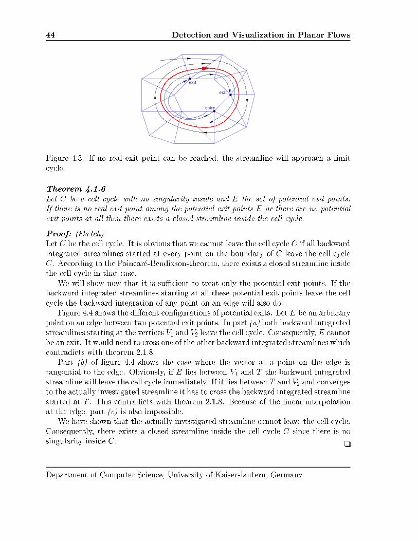
44 Dete tion and Visualization in Planar Flowsexit
exit
entry
Figure 4.3: If no real exit point an be rea hed, the streamline will approa h a limit y le.Theorem 4.1.6Let C be a ell y le with no singularity inside and E the set of potential exit points.If there is no real exit point among the potential exit points E or there are no potentialexit points at all then there exists a losed streamline inside the ell y le.Proof: (Sket h)Let C be the ell y le. It is obvious that we annot leave the ell y le C if all ba kwardintegrated streamlines started at every point on the boundary of C leave the ell y leC. A ording to the Poin ar�e-Bendixson-theorem, there exists a losed streamline insidethe ell y le in that ase.We will show now that it is suÆ ient to treat only the potential exit points. If theba kward integrated streamlines starting at all these potential exit points leave the ell y le the ba kward integration of any point on an edge will also do.Figure 4.4 shows the di�erent on�gurations of potential exits. Let E be an arbitrarypoint on an edge between two potential exit points. In part (a) both ba kward integratedstreamlines starting at the verti es V1 and V2 leave the ell y le. Consequently, E annotbe an exit. It would need to ross one of the other ba kward integrated streamlines whi h ontradi ts with theorem 2.1.8.Part (b) of �gure 4.4 shows the ase where the ve tor at a point on the edge istangential to the edge. Obviously, if E lies between V1 and T the ba kward integratedstreamline will leave the ell y le immediately. If it lies between T and V2 and onvergesto the a tually investigated streamline it has to ross the ba kward integrated streamlinestarted at T . This ontradi ts with theorem 2.1.8. Be ause of the linear interpolationat the edge, part ( ) is also impossible.We have shown that the a tually investigated streamline annot leave the ell y le.Consequently, there exists a losed streamline inside the ell y le C sin e there is nosingularity inside C. ❏Department of Computer S ien e, University of Kaiserslautern, Germany

Closed Streamlines in Flow Visualization 45backward integration
1 2V VE
actual streamline
leaves cell cycle
(a)1 2V VT E
actual streamline
backward integration
leaves cell cycle
(b)backward integration
1 2V VE
actual streamline( ) backward integration
1 2V VE
actual streamline(d)backward integration
1 2V VT E
actual streamline(e)Figure 4.4: Di�erent ases of potential exits. (a) and (b) is impossible be ause stream-lines annot ross ea h other, ( ) ontradi ts with the linear interpolation on an edge,in (d) and (e) both ba kward integrations onverge to the a tual streamline so that thepoint E is a real exit.Department of Computer S ien e, University of Kaiserslautern, Germany

46 Dete tion and Visualization in Planar FlowsRemark 4.1.7To get a possible on�guration the ba kward integration starting at the vertex V1 mustalso onverge to the streamline be ause it annot ross the ba kward integration startingat point E as in part (d) of �gure 4.4. Part (e) explains why we also need to investigatethe tangential ase. If we start a ba kward integrated streamline at point E it onvergestowards the a tually investigated streamline. But if we only onsider the verti es of theedge, both exit points may be no real exit points. Therefore we also have to start aba kward integrated streamline at the point T , where the ve tor �eld is tangential to theedge, to �gure out that we leave the ell y le at this edge. On the other hand, a ba kwardintegrated streamline starting at any point between V1 and T immediately leaves the ell y le due to the linear interpolation.4.1.2 AlgorithmWith theorem 4.1.6 we are able to des ribe our algorithm in detail. It mainly onsistsof the same three di�erent states:➊ streamline integration: identifying one ell hange after the other, he k at ea h ell if we omplete a ell y le.➋ he king for exits: going ba kwards through the rossed ells and looking forpotential exit points.➌ validating exit: integrating ba kwards a urve from potential exit through thewhole ell y le.
Start critical point
boundary
limit cycle
exit valid
foundexitstartsoutside
potential exit
(3) Validating Exit
(2) Checkingfor Exit
(1) StreamlineIntegration
cell cycledetected
Figure 4.5: The UML state diagram of our algorithm.The algorithm swit hes its states after the events shown in the state diagram in�gure 4.5. We use a standard integration method to ompute the streamline, �rst. InDepartment of Computer S ien e, University of Kaiserslautern, Germany

Closed Streamlines in Flow Visualization 47this step we only he k for ell y les. This saves omputational time sin e the he kingof all the exits is rather expensive. If we dete t a ell y le we have to �nd all potentialexit points. After that we need to validate ea h of the potential exit points to �gure outif there is a real exit point among them. If this is the ase we did not run into a losedstreamline yet. Therefore we ontinue with the standard integration. The algorithmexits if we ould not �nd a real exit point among all the potential exit points or if werea hed a riti al point or the boundary of the ve tor �eld.Remark 4.1.8Theorem 4.1.6 guarantees that our algorithm dete ts losed streamlines if we he k everypotential exit point.
Figure 4.6: Exits of a ell y le.Figure 4.6 shows a real example of our algorithm. There we start a streamline nearthe sour e in the enter of the �gure. This streamline spirals until we �nd the �rst ell y le. We stopped the integration there for this example. The �gure also shows all exitsand its ba kward integrated streamlines. The streamline itself is olored bla k. The gridis displayed in a lighter olor. In this example, every potential exit point is shown. We an see that potential exit points whi h are passed by a ba kward integrated streamlinedo not ne essarily need to be investigated be ause if the ba kward integrated streamlineleaves the ell y le the other one will also do. Figure 4.7 shows this in detail. Therethe ba kward integrated streamline starting at Exit 2 also has to leave the ell y lebe ause it annot ross the ba kward integrated streamline starting at Exit 1. In theDepartment of Computer S ien e, University of Kaiserslautern, Germany

48 Dete tion and Visualization in Planar Flows
Figure 4.7: Exit of the ell y le whi h does not need to be investigated.other ase, where the ba kward integrated streamline started at Exit 1 stays inside the ell y le, we have to ontinue the a tually investigated streamline, anyway.Sin e the streamline spirals from the inner region to the outside, we only have to onsider the potential exits in that dire tion. In the example, every ba kward integratedstreamline leaves the ell y le. Consequently, there is a limit y le in this ell y lewhi h an be lo alized as des ribed in the next se tion.4.2 Exa t Lo ation of Closed StreamlinesSin e we know a region that is never left by the streamline we an �nd the exa t positionof the losed streamline using the Poin ar�e map. This map is des ribed in detail in thesubse tion 2.5.2.To �nd the exa t position of the losed streamline we an use the edge where wedete ted the ell y le as a Poin ar�e se tion. Then we only have to �nd the �xed pointof the Poin ar�e map. We use a binary sear h to �nd this �xed point: we divide the edgewhere we dete ted the ell y le into two parts. At the mid point we start a streamline tosee whi h part of the edge is interse ted by the streamline after one full turn. Sin e thestreamline annot leave the ell y le, it is guaranteed that the streamline interse ts onepart of the edge. Then, this part is subdivided again and we start another streamlineat the mid point. This pro ess ontinues until we are lose enough to the �xed point ofthe Poin ar�e map. We use the length of the part of the edge as a stopping riterion.This �xed point gives us a point lying on the losed streamline. If we start anotherstreamline at that point this streamline will follow the losed streamline we are lookingfor. After one turn, i.e. after rea hing the start point again, we know the exa t lo ationof the losed streamline.Department of Computer S ien e, University of Kaiserslautern, Germany

Closed Streamlines in Flow Visualization 494.3 Results
Figure 4.8: Simple ve tor �eld with limit y le.The �rst example is a ve tor �eld that ontains only one losed streamline. It issampled on a regular grid using a slightly hanged Van der Pol's equation. The de�ningequation for the ve tor �eld V isV�xy� = �y � x3 + �x�x � : (4.1)
Figure 4.9: Simple ve tor �eld with no limit y le.Department of Computer S ien e, University of Kaiserslautern, Germany

50 Dete tion and Visualization in Planar FlowsA ording to Hirs h and Smale[HS74℄ a limit y le o urs if we set 0 < � � 1.An analysis of the �eld shows that we have a sour e at (0; 0). When starting ouralgorithm near that singularity it integrates the streamline until it dete ts the limit y leas shown in �gure 4.8. Figure 4.8 also in ludes the hedgehog of the ve tor �eld, a glyphvisualization method where we use arrows representing the ve tors at the orrespondingposition. The arrows are twi e as long as the ve tors of the �eld.In �gure 4.9, we investigate a ve tor �eld whi h spirals from the singularity to theouter regions. Again, we used equation 4.1 but we set � = �0:02 to ompute theve tor �eld. Consequently, there is no limit y le in the ve tor �eld. Our algorithm orre tly fails to dete t one, when started near the singularity at (0; 0) and ontinuesthe streamline omputation until it rea hes the boundary of the ve tor �eld. Here, alsothe hedgehog of the ve tor �eld is displayed s aled by a fa tor of two.
Figure 4.10: Vorti ity ve tor �eld of a turbulent ow { hedgehog.Department of Computer S ien e, University of Kaiserslautern, Germany

Closed Streamlines in Flow Visualization 51
Figure 4.11: Vorti ity ve tor �eld of a turbulent ow { limit y les.
Figure 4.12: Vorti ity ve tor �eld visualized by the topologi al skeleton in luding losedstreamlines. Department of Computer S ien e, University of Kaiserslautern, Germany

52 Dete tion and Visualization in Planar FlowsThe third example is a simulation of a swirling jet with an in ow into a steadymedium. The simulation originally resulted in a three dimensional ve tor �eld but weused a utting plane and proje ted the ve tors onto this plane to get a two dimensional�eld. This dataset was provided by Prof. Kollmann from the me hani al engineeringdepartment at the University of California at Davis. In this appli ation one is interestedin investigating the turbulen e of the ve tor �eld and in regions where the uid staysvery long. This is ne essary be ause some hemi al rea tions need a spe ial amount oftime. These regions an be lo ated by �nding losed streamlines. Figure 4.10 shows thehedgehog of that ve tor �eld s aled by a fa tor of two. In �gure 4.11 one an see some ofthe losed streamlines dete ted by our algorithm. All these limit y les are lo ated in theupper region of the ve tor �eld. Additionally �gure 4.11 in ludes the hedgehog wherethe arrows representing the ve tors are four times longer than the orresponding ve tor.Figure 4.12 shows all losed streamlines of this ve tor �eld in luding the topologi alskeleton.To ompare our enhan ements with usual streamline omputation methods, we im-plemented an algorithm whi h omputes the topologi al skeleton as des ribed in [HH91℄.Therefore we have to determine the singularities. Then we start a streamline at ea hsaddle point displa ed a little bit in positive and negative eigendire tion of both eigen-ve tors. Remind that our algorithm does not need any exit onditions other than thedete tion of losed streamlines or rea hing a singularity or the border of the data!To get an idea of the omputational ost of our method we also implemented asimple ODE solver to ompute the streamlines. The ve tor �eld shown in �gure 4.10 ontains 337 singularities. The algorithm using a simple ODE solver needed 738 se ondsto ompute the topologi al skeleton on a Pentium II 350 MHz. Using our streamlineintegration method, whi h uses the same ODE solver but he ks for limit y les, weonly needed 604 se onds on the same system whi h is 18 per ent faster! The reason forthat is that we do not need to wait until the ODE solver rea hes a ertain number ofsteps if we run into a limit y le. This saves some time whi h we an use to he k forlimit y les.4.4 LimitationsIf more than one losed streamline rosses the same ell, the algorithm may fail to dete tthese losed streamlines. For instan e, there is a stru tural unstable on�guration withone losed streamline inside the other. One losed streamline a ts like a sour e, letssay the inner one, while the other one behaves like a sink so that the ow starts at the�rst and is attra ted by the se ond one. Sin e there is an out ow out of the ell thealgorithm annot distinguish between a regular out ow and this on�guration.Figure 4.13 shows an example for su h a on�guration. The ow dire tion inside the�rst losed streamline is the same than behind the se ond one. It looks the same as ifDepartment of Computer S ien e, University of Kaiserslautern, Germany

Closed Streamlines in Flow Visualization 53
Figure 4.13: Unstable losed streamlines.there are no losed streamlines at all. Consequently, the algorithm fails to dete t both losed streamlines.
Department of Computer S ien e, University of Kaiserslautern, Germany

54 Dete tion and Visualization in Planar Flows
Department of Computer S ien e, University of Kaiserslautern, Germany
Closed Streamlines in Flow Visualization 55Chapter 5Parallel Dete tion of ClosedStreamlinesTo determine the losed streamlines of a ve tor �eld many streamlines have to be om-puted. In fa t, we ompute the topologi al skeleton. This graph leads us to the losedstreamlines. Sin e the number of streamlines may be large depending on the given ve -tor �eld, this may take several minutes or even hours, espe ially sin e we also have to ompute even more ba kward integrated streamlines. Therefore we reated a parallelversion of this algorithm to de rease omputational time by distributing the streamline omputation to several lients. Some more information on on urrent programming anbe found in the literature [S h97℄[Mul93℄ [Ung97℄[Aga89℄.First, we des ribe some parallel ma hines that an be used for our algorithm. Thentwo di�erent parallelization methodologies are dis ussed in the next se tion. In the endof this hapter we show the results in luding di�erent timings on several test systems.5.1 Parallel Ma hinesIn this se tion we des ribe brie y some parallel ma hines, the Cray/SGI T3E, the IBMRS/6000 SP, and Linux lusters. The �rst one uses a distributed shared memory on eptwhile the other two ones do not share their memory at all.5.1.1 Cray/SGI T3EThe Cray/SGI T3E is available sin e 1996. It is a distributed shared memory systemwhere every node shares its memory with all the others. It uses a virtual address spa eto a ess the memory that is spread among all nodes. The pro essor used for the nodes isthe DEC Alpha pro essor 21164. This pro essor onsists of two integer and two oatingpoint units with IEEE 64 bit arithmeti . It has an eight KB �rst level and 96 KB se ondDepartment of Computer S ien e, University of Kaiserslautern, Germany

56 Parallel Dete tion of Closed Streamlineslevel a he dire tly on the hip.The GigaRing te hnology based on the IEEE SCI standard is used to onne t thenodes. Every node is bi-dire tional onne ted to its neighbor in a three dimensionalnetwork topology.5.1.2 IBM RS/6000 SPThe IBM RS/6000 SP uses POWER4 mi ropro essors. This type of pro essor has anSMP-on-a- hip design. It onsists of two 1.3 GHz pro essors in luding se ond level a he dire tly on one hip. Every node has its own memory. So the parallel programhas to use a message passing system as for instan e PVM or MPI.
N15N14N13N12
N11N10N9N8
N7N6N5N4
N3N2N1N0
Figure 5.1: HPS basi element of an IBM RS/6000 SP for 16 nodes.Up to sixteen nodes are grouped together in a network on�guration as shown in�gure 5.1 using high performan e swit hes (HPS). If more than sixteen nodes are usedseveral of these groups have to be inter onne ted.5.1.3 Linux ClustersWith Linux lusters there are no restri tions on erning network topology, memory, orCPU speed. Almost every standard PC omponent an be used in a Linux luster.Even several desktop Linux omputers that are onne ted through an Ethernet an beDepartment of Computer S ien e, University of Kaiserslautern, Germany

Closed Streamlines in Flow Visualization 57 alled a Linux luster. But usually the network is the bottlene k in su h a system.Therefore faster network devi es like for instan e a GigaBit network devi e or Myrinethost interfa e is used. A at, tree shaped network topology is possible for a Linux luster. But espe ially with a greater number of nodes a network with routes from anyto any other node is desirable to avoid ollisions and fa ilitate faster transfers.Be ause of their low pri es and the great s alability Linux lusters be ome more andmore popular. They also appear nowadays in the list of the top 500 Super omputerSites.5.1.4 Comparison Cray/SGI T3E IBM RS/6000 SP Linux ClusterPro essor type DEC Alpha 21164 p690 server (dual) e.g. AthlonNumber of pro essors up to 2176 up to 16 unlimitedMemory size (per node) 512 MB { up to 3 GBClo k speed (per node) up to 675 MHz up to 1.3 GHz up to 2GHzNetwork bandwidth 500 MB/s 500 MB/s up to 250 MB/sPeak Performan e 3 TFLOPS 2.6 TFLOPS unlimitedFigure 5.2: Te hni al spe i� ations of di�erent parallel ma hines.The main advantage of Linux lusters is the low pri e of standard PC omponents. Itis very extendable be ause there is no limit in the number of nodes used in the luster. Inprin iple, you only have to add a new omputer to the network to in rease omputationalpower. The pro essors are faster than the ones used for both other parallel ma hines.The advantage of both, the Cray/SGI T3E and the IBM RS/6000 SP, is the fasternetwork. Both ommer ial systems are limited with respe t to extendability. Figure 5.2shows some te hni al spe i� ations of the three di�erent parallel ma hines. Altogether,a Linux luster is the best way to get a great performan e at a low pri e.5.2 Parallel AlgorithmTo ompute the losed streamlines there are two di�erent tasks. First, we have to ompute the riti al points in the given ve tor �eld. The se ond task is to ompute the losed streamlines by determining the topologi al skeleton. The next two subse tionsdes ribe these tasks in detail.Department of Computer S ien e, University of Kaiserslautern, Germany

58 Parallel Dete tion of Closed Streamlines5.2.1 Parallel Computing of Criti al PointsTo parallelize this algorithm we have to ompute all the riti al points that are presentin the ve tor �eld, �rst. Sin e we only need the data of the ells, i.e. the position ofthe verti es and the ve tors at these verti es, to determine if there exists a riti al pointinside the ell and where it is lo ated, we an transfer these tasks to the various lientsof the luster. When the lients re eive the index of a ell they ompute the riti alpoint and return the position and its type, if they have found one, to the server. Alltasks are ontrolled by a s heduler whi h is a part of the server.receive task
execute task
send resultreceive result
create task
get next task
spool task
ClientServerScheduler
Figure 5.3: S heduling of the tasks.The s heduling of the tasks works as follows: the server reates one task for ea h ell ontaining the index of this ell and queues it in the s heduler. The s heduler itself he ks if there are still tasks left and if there is any lient that has �nished its task yet.If there is more than one lient without an a tive job, the fastest is hosen. Then thenext task is sent to this lient. The lient re eives this task, omputes the riti al pointand sends it, if it has found one, ba k to the server and tells the s heduler that it has�nished its job. Sin e the amount of data to ontrol the lients and transfer the riti alpoints ba k to the server is very low, we an fully bene�t from the performan e of ea h lient.5.2.2 Determining Closed Streamlines in ParallelA ording to the motivation there exist two di�erent approa hes for parallelization. Weexperimented with both approa hes to �nd the best one. There are dis ussed in detailin the following.Department of Computer S ien e, University of Kaiserslautern, Germany

Closed Streamlines in Flow Visualization 59Server
Client2 Client3 ClientN
Dataset Scheduler
Client1
Cache Cache Cache CacheFigure 5.4: Con�guration of the parallel program.5.2.2.1 Subdivision Approa hIn our �rst approa h every lient got its data from the server. Computing streamlines isa global task sin e it is not known whi h region of the ve tor �eld this streamline may ross. Therefore it is not possible to simply subdivide the whole dataset into severalregions. If we want to subdivide into several regions we have to restart the streamlinein another task if it leaves su h a region. This usually results in a poor load balan ingsin e it is likely that there are regions that are rossed by only few streamlines. It ispossible to swit h regions in a parti ular task. But again, we do not know if a streamline rossed exa tly that region we just ex hanged.Therefore we tried a di�erent approa h where ea h request to the dataset on one ofthe lients results in questioning the server using PVM[GBD+94℄. Figure 5.4 shows the on�guration. We use a hes to avoid asking the server for the same data repeatedly. Butdue to the slow network onne tion and the long start-up time for ommuni ating underPVM the transfer of the data took more time than the omputation of the streamlineeven when we used a GigaBit- onne tion. As a result the parallel version using su h asubdivision approa h uses more time than the sequential version.5.2.2.2 Task Driven Approa hAfter we have omputed all riti al points, we start streamlines at ea h saddle point inpositive and negative eigendire tion with respe t to the matrix of the linear interpolantand he k for losed streamlines while omputing the streamlines as previously des ribed.Computing streamlines is not a lo al task sin e the streamlines may ross any regionof the ow. Therefore we do not subdivide the data into several blo ks like in somerendering tasks [IAO94℄. Our implementation uses an approa h where we reate severaltasks ea h of them representing the whole omputation of one streamline starting at agiven position. Then we use the s heduler to distribute the tasks to the various lientsof our luster.Sin e the data of the ve tor �eld in luding o tree and the program �t into 64 MBDepartment of Computer S ien e, University of Kaiserslautern, Germany

60 Parallel Dete tion of Closed StreamlinesServer
Client1 Client2 Client3 ClientN
Dataset Scheduler
Dataset Dataset DatasetDatasetFigure 5.5: Con�guration of the parallel program.of RAM we de ided to use a on�guration where every lient loads the whole datasetinto its own memory. This fa ilitates the fastest possible a ess to the data. Sin e theserver and every lient load the data at the same time there is no time lost be auseotherwise the lients would simply wait for the server until it has loaded the dataset.When dealing with larger datasets we have to use an out of ore method whi h will bedone in the future.Sin e we want to spread tasks that represent the whole omputation of one stream-line, ea h task ontains two items: a point where the streamline has to start and theintegration dire tion. The other data that is needed for the omputation is alreadypresent at ea h lient be ause the lient has loaded the whole dataset yet. Due to theminimal amount of data of ea h task the ommuni ation ost whi h is produ ed bymigrating tasks is very low.To distribute the tasks to the various lients we use the previously des ribed s hed-uler: the server determines the start positions of the streamline using ea h saddle pointfound in the ve tor �eld. Then a task ontaining this start position and the integrationdire tion is reated and spooled into the queue of the s heduler, while the s hedulersends the next job to the fastest lient that has no a tive job. The lient re eives thistask, sear hes for losed streamlines and sends it, if it has found one, ba k to the server.Again, the amount of data to ontrol the lients and transfer the losed streamlinesba k to the server is very low, so that we an fully bene�t from the performan e of ea h lient.5.3 ResultsOur algorithm is implemented in C++, while the server ommuni ates with the lientsusing PVM[GBD+94℄. The di�erent tasks are en apsulated in C++- lasses. This fa- ilitates that the tasks an transfer themselves to the lient on demand and the lientsonly need to all a method to exe ute the re eived task.To test the performan e of our implementation we mainly use two di�erent systems.Department of Computer S ien e, University of Kaiserslautern, Germany

Closed Streamlines in Flow Visualization 61One is a Linux luster onsisting of seven lients. Ea h node is equipped with anAMD Duron 600 or AMD Duron 700 pro essor and 64 MB of RAM. The server is amultipro essor omputer with two Pentium III 500 pro essors. The se ond system isbased on some of our desktop omputers with a Pentium II 350. We use Linux andnormal PC omponents sin e this is a heap way to get a great performan e omparedto other parallel omputers. In order to get a more heterogeneous on�guration we mixboth systems by using all Linux omputers available in our group for a last performan etest.As a test dataset we use the same simulated dataset as in the previous hapter. Theve tor �eld has 362 riti al points and for the topology in luding losed streamlinesabout six hundred streamlines have to be omputed.Pro essor Floating-point indexPentium II 350 2.404Pentium III 500 3.561AMD Athlon 650 5.163AMD Duron 600 4.768AMD Duron 700 5.547Intel Celeron 800 6.125AMD Thunderbird 1400 11.227Figure 5.6: Floating-point indi es of the di�erent pro essors.To determine the optimal timing of our algorithm we used the ben hmark utilitynben h1 in order to get a suitable ratio between the speeds of the pro essors. Nben h isa port to Linux/Unix of release 2 of BYTEMagazine's BYTEmark ben hmark program2.We omputed the oating-point index of ea h pro essor whi h gives the relative speedof the oating-point unit ompared to an AMD K6-233 pro essor. The results an befound in �gure 5.6. Using these values we omputed the oating-point index of the wholeparallel ma hine by summing up the indi es orresponding to the involved pro essorsand al ulated the optimal runtime by negle ting the ommuni ation ost between serverand lients.Figures 5.7 and 5.8 show the timings on the desktop omputers. The luster onsistsof up to �ve ma hines. The optimal timings are displayed using a dashed line while thereal timings are shown by a solid line. This on�guration is very suitable for testing thes alability of our implementation be ause every omputer has identi al performan e.Obviously, the omputation time is halved if the number of pro essors is doubled whi hindi ates a good s alability of our implementation.1http://www.tux.org/~mayer/linux/bmark.html2http://www.byte. om/bmark/bmark.htmDepartment of Computer S ien e, University of Kaiserslautern, Germany

62 Parallel Dete tion of Closed Streamlines
2 51 3 4processors
time
100
600
300
400
500
200
Figure 5.7: Time needed to ompute losed streamlines using Pentium PII-350 pro es-sors displayed as graph. # CPUs Time Optimum1 612s |2 306s 306s3 205s 204s4 158s 153s5 134s 122sFigure 5.8: Time needed to ompute losed streamlines using Pentium PII-350 pro es-sors shown in a table.The timings of the algorithm running on our Linux luster with up to seven lientsis displayed in �gures 5.9 and 5.10. Again, the optimal timings are displayed using adashed line while the real timings are shown by a solid line. Sin e the server has twopro essors there are always running at least two tasks at the same time on this ma hine.Adding more lients to the Linux luster the time needed for the algorithm is redu ed orrespondingly to the speed of its pro essor. Again, we an see that we nearly bene�tfrom the full performan e of ea h lient due to the minimal ommuni ation betweenserver and lient as an be seen from the di�eren e between the optimal and the realtimings.In our next test we also used the Linux desktop ma hines in all the oÆ es of ourvisualization group. This resulted in a parallel ma hine onsisting of six Pentium II-350, two AMD Athlon 650, one dual pro essor ma hine with two Pentium III-500, fourAMD Duron 600, and three AMD Duron 700. Altogether, the algorithm used seventeenDepartment of Computer S ien e, University of Kaiserslautern, Germany

Closed Streamlines in Flow Visualization 63time
300
100
200
1 2 3 4 5 6 7 9 10 11 13 14 15 16 178 12processors
3018 19 20 21 22 23 24 25 26 27 28 29Figure 5.9: Time needed to ompute losed streamlines using a Linux luster with AMDDuron 600 and AMD Duron 700 pro essors displayed as graph.# CPUs Time Optimum2 224s |3 138s 134s4 99s 96s5 77s 74s6 63s 61s7 53s 50s8 46s 43s9 39s 37s17 28s 24s30 17s 9sFigure 5.10: Time needed to ompute losed streamlines using a Linux luster withAMD Duron 600 and AMD Duron 700 pro essors shown in a table.pro essors and it took 28 se onds to ompute all losed streamlines that are present inour test dataset. As expe ted, this is faster than using the luster alone orresponding tothe speed of the pro essors and slightly slower than the optimal runtime of 24 se onds.This also tests our implementation in a more heterogeneous parallel ma hine due to thedi�erent speeds of the pro essors. It shows that we an de rease the time needed forthe omputation by adding more pro essors no matter what sort of ma hine it is.Then we also added the Linux ma hines in our student rooms for a last test. Theseare �ve ma hines equipped with an Intel Celeron 800, two ma hines with a PentiumIII-500, and six with an AMD Thunderbird 1400 pro essor. So we end up with 30Department of Computer S ien e, University of Kaiserslautern, Germany

64 Parallel Dete tion of Closed Streamlinespro essors. Our algorithm needed 17 se onds. Compared to the optimal timing of 9se onds this is a little bit too slow. This is due to the slow network onne tion. Be auseall omputers reside in di�erent areas of our working group and several other pro essessu h as network �le system also use this network we do not have the full bandwidthavailable. Consequently, the ommuni ation ost is not negle table anymore so that thereal and the optimal timings di�er.
Department of Computer S ien e, University of Kaiserslautern, Germany

Closed Streamlines in Flow Visualization 65Chapter 6Closed Streamlines inTime-Dependent FlowsWhen dealing with losed streamlines one question o urs: how does a losed streamlineemerge? Inspired by the books of Abraham and Shaw[AS82℄ [AS83℄ [AS84℄ [AS88℄ wevisualize the evolution of a losed streamline in a planar unsteady ow. We use the thirddimension to represent the time. The evolution of a losed streamline an be shown asa tube shaped visulization for the losed streamlines in the various timesteps.The singularities are used as a starting point for our investigations. Therefore webrie y des ribe the tra king of the singularities in the next se tion. This work was doneby Tri o he et al. [TSH01℄. Then we show how to �nd and follow a losed streamlineover time. In the end we explain the results of our algorithm and explain the limitationsof our method.6.1 Tra king Criti al PointsWhen dealing with time-dependent two-dimensional ows we an use the third dimen-sion to represent time as des ribed in subse tion 2.2.4. For tra king the losed stream-lines we �rst determine the behavior of the riti al points. For a given ell, the asso iatedinterpolant ontains, for ea h value of time t, a single riti al point. This is due to theaÆne linear nature inside the triangles of its restri tion to any time plane. Letting thetime parameter t move from ti to ti+1, the riti al point position des ribes a 3D urve.A detailed des ription of how to �nd the paths of the riti al points an be found in thearti le of Tri o he et al. [TSH01℄.Department of Computer S ien e, University of Kaiserslautern, Germany

66 Closed Streamlines in Time-Dependent Flows
Figure 6.1: Closed streamlines found by the algorithm.6.2 Following Closed StreamlinesAfter tra king the singularities, we analyze the ve tor �eld in dis rete timesteps. Theremust be a riti al point inside ea h losed streamline. Therefore, we use the riti al pointpath ontaining a Hopf bifur ation as a starting point for our streamline algorithm fromse tion 4.1 whi h dete ts the losed streamline if it exists. We follow the riti al pointpath in dis rete steps in positive and negative dire tions starting at the bifur ation.After we have found the ell y le ontaining the losed streamline we �nd the exa tposition using the Poin ar�e-map from se tion 4.2. As a last test we have to he k ifthe losed streamline really surrounds the riti al point. This is ne essary be ause thestreamline may have ran into another losed streamline in a totally di�erent region of the ow. Obviously, losed streamlines surrounding the riti al point o ur only in one ofthe two temporal dire tions. We ontinue by stepping forward in the temporal dire tionuntil the losed streamlines rea h either another bifur ation whi h breaks them up orthe border of the grid.Figure 6.1 shows the result of this step. Here we have found the losed streamlinesat various timesteps. The losed streamlines are approximated by several line segments.The paths of the riti al points are also shown using the same olors as in the originalpaper [TSH01℄. The Hopf bifur ation, where we started to dete t the losed stream-lines, is marked with a yellow sphere. The di�erent bifur ation types are des ribed inse tion 2.8. In this example the life y le of the losed streamline is started by a HopfDepartment of Computer S ien e, University of Kaiserslautern, Germany

Closed Streamlines in Flow Visualization 67
Figure 6.2: Closed streamlines visualized as a tube over time.bifur ation and terminated by a Periodi Blue Sky in 2D bifur ation.To visualize the evolution of losed streamlines, we onstru t tubes from the various losed streamlines similar to the pi tures by Abraham and Shaw [AS88℄. We onstru tsurfa es onsisting of triangles whi h onne t the approximating line segments of the losed streamlines. The bifur ation point is onne ted to the tube using a paraboli surfa e approximated with triangles. The result is shown in �gure 6.2.6.3 ResultsTo test our method, we have reated a syntheti ve tor �eld ontaining four riti alpoints. The position of the riti al points is a fun tion of time, des ribing losed urvesin the plane. We have sampled this ve tor �eld on a triangular point set for severalvalues of the time parameter. The rotation of the riti al points (ea h with a spe i� frequen y) entails many stru tural hanges for the topology. This is very interesting forour purpose sin e all di�erent types of bifur ations whi h reate losed streamlines arepresent.Figure 6.3 shows the result of our algorithm, where the losed streamlines are shownas red tubes. The upper one and the one on the right are started and terminated by HopfDepartment of Computer S ien e, University of Kaiserslautern, Germany

68 Closed Streamlines in Time-Dependent Flows
Figure 6.3: Closed streamlines found in a syntheti test dataset.
Figure 6.4: Detailed view of a Hopf bifur ation.bifur ations { shown as a yellow sphere { while the lower losed streamline starts at aHopf bifur ation and is terminated by a Periodi Blue Sky in 2D bifur ation. Sin e thereis a riti al point inside the ell y le, i.e. the saddle, the ow behaves totally di�erentdepending on where a streamline passes the saddle. Therefore the exa t lo alizationfails when we are too lose to the riti al point.Figures 6.4 and 6.5 show some detailed views of the di�erent bifur ations. Also someDepartment of Computer S ien e, University of Kaiserslautern, Germany

Closed Streamlines in Flow Visualization 69
Figure 6.5: Detailed view of a Periodi Blue Sky in 2D bifur ation.streamlines are drawn to show how these streamlines ir le around the limit y le butnever ross it. Figure 6.4 is a losed streamline started by a Hopf bifur ation. Thebifur ation is lo ated in the lower left orner. In �gure 6.5 the losed streamline isstarted by a Hopf bifur ation lo ated in the upper left orner. It grows in size until it isterminated by a Periodi Blue Sky in 2D bifur ation. Consequently, the tube visualizingthe evolution of the losed streamline does not get losed.Another dataset we used is a simulation of a swirling jet with an in ow into a steadymedium. The simulation uses a ylindri al domain and assumes rotational symmetry, sothat we are left with a two-dimensional ve tor �eld on a plane through the enter axis ofthe ylinder. In this appli ation one is interested in investigating the turbulen e of theve tor �eld and in regions where the uid stays very long. Swirling jets play a signi� antrole in many ombustion pro esses. It is important to �nd su h re ir ulation regionsindi ated by losed instantaneous streamlines. To avoid visual lutter we use only apart of the dataset for our visualization. Figure 6.6 shows the result of our algorithm.The riti al point paths are also shown where saddles are olored red, sinks are green,and sour es are visualized using blue olor. Obviously, in regions where only one saddlepoint is involved, we annot �nd any losed streamline due to the types of bifur ationsexplained in se tion 2.8. Most of the losed streamlines emerge at Hopf bifur ationswhi h are marked with a yellow sphere. Therefore, losed streamlines are found wheresour es and sinks alternate while time propagates, so that we are able to identify theregions where the uid stays very long.Department of Computer S ien e, University of Kaiserslautern, Germany
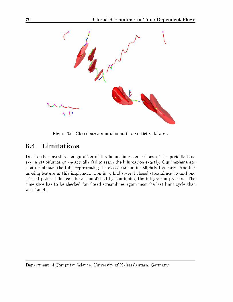
70 Closed Streamlines in Time-Dependent Flows
Figure 6.6: Closed streamlines found in a vorti ity dataset.6.4 LimitationsDue to the unstable on�guration of the homo lini onne tions of the periodi bluesky in 2D bifur ation we a tually fail to rea h the bifur ation exa tly. Our implementa-tion terminates the tube representing the losed streamline slightly too early. Anothermissing feature in this implementation is to �nd several losed streamlines around one riti al point. This an be a omplished by ontinuing the integration pro ess. Thetime sli e has to be he ked for losed streamlines again near the last limit y le thatwas found.
Department of Computer S ien e, University of Kaiserslautern, Germany

Closed Streamlines in Flow Visualization 71Chapter 7Closed Streamlines in 3D Ve torFieldsClosed streamlines an be found in three dimensional ve tor �elds also. For instan e,the Terrestrial Planet Finder Mission of NASA deals with stable manifolds where 3Dperiodi halo orbits play an important role. These orbits are nothing else than losedstreamlines in a three dimensional ve tor �eld. Figure 7.1 shows an example.
Figure 7.1: Terrestrial Planet Finder Mission (image ourtesy of Ken Museth,Calte h[MBL01℄).The next se tion des ribes how to dete t losed streamlines in three dimensionalve tor �elds. It shows the di�eren es between the two dimensional ase both in theoryand the algorithm itself. In the end we present the results of the algorithm.Department of Computer S ien e, University of Kaiserslautern, Germany

72 Closed Streamlines in 3D Ve tor Fields
Figure 7.2: Ba kward integrated surfa e.7.1 Dete ting Closed Streamlines in 3D Ve torFieldsAlthough the prin iple to dete t losed streamlines in a three dimensional ve tor �eldis similar to the two dimensional ase there are some di�eren es. We will des ribe thetheoreti al and algorithmi di�eren es and similarities in the next two subse tions.7.1.1 TheoryThe data is given on a tetrahedral grid. But the prin iple should work on other elltypes as well. The dete tion of a ell y le works the same as in de�nition 4.1.2. Of ourse, the ells are three dimensional in this ase. To he k if we an leave the ell y le we have to onsider every ba kward integrated streamline starting at an arbitrarypoint on a fa e of the boundary of the ell y le. Looking at the edges of a fa e we ansee dire tly that it is not suÆ ient to just integrate streamlines ba kwards. Figure 7.2shows an example. We integrated a streamsurfa e ba kwards starting at an edge ofthe ell y le. The streamlines starting at the verti es of that edge leave the ell y leearlier than the omplete surfa e. So it may be possible that a part of the streamsurfa estays inside the ell y le although the ba kward integrated streamlines starting at theverti es leave it. Consequently, we have to �nd another de�nition for exits.Department of Computer S ien e, University of Kaiserslautern, Germany

Closed Streamlines in Flow Visualization 73De�nition 7.1.1 (Potential Exit Edges)Let C be a ell y le in a given tetrahedral grid G as in De�nition 4.1.2. Then we allevery edge at the boundary of the ell y le a potential exit edge. Analogue to the twodimensional ase we de�ne a line on a boundary fa e where the ve tor �eld is tangentialto the fa e as a potential exit edge also.Due to the fa t that we use linear interpolation inside the tetrahedrons we an showthat there will be at least a straight line on the fa e where the ve tor �eld is tangentialto the fa e or the whole fa e is tangential to the ve tor �eld.Theorem 7.1.2Let F be a triangular fa e of a tetrahedral. The ve tors v1, v2, and v3 are the ve torvalues and p1, p2, and p3 the positions of the verti es of the fa e F . The ve tors insidethe tetrahedron are interpolated linearly. Then all ve tors that are tangential to the fa eare on a straight line or all ve tors inside the fa e are tangential.Proof:Let v1, v2, v3, p1, p2, and p3 the ve tors of respe tively positions at the verti es of thefa e F . Let n be an orthogonal ve tor to the fa e F . We an interpolate a ve tor insidethe fa e F by using the bary entri oordinates:v = � � v1 + � � v2 + � v3Every ve tor that is tangential to the fa e F is orthogonal to the ve tor n. Therefore:n � v = �n � v1 + �n � v2 + n � v3A property of the bary entri oordinates is that they sum up to 1:� + � + = 1So we have two equations and three variables. This leads to an at least one dimensionalsolution of linear equations if there is any solution. ❏Remark 7.1.3Be ause of theorem 7.1.2 we do not need to onsider any isolated point on a fa e wherethe ve tor �eld is tangential to the fa e be ause this annot o ur.When dealing with edges as exits we have to ompute a streamsurfa e instead ofstreamlines to onsider every point on an exit edge. This leads us to the followingnotation.Notation 7.1.4 (Ba kward integrated streamsurfa e)We use the term ba kward integrated streamsurfa e to des ribe the streamsurfa ewe integrate by inverting the ve tors of the ve tor �eld starting at a potential exit edgein order to validate this exit edge.Department of Computer S ien e, University of Kaiserslautern, Germany

74 Closed Streamlines in 3D Ve tor FieldsAnalogue to de�nition 4.1.5 we de�ne real exit edges.De�nition 7.1.5 (Real exit edge)Let E be a potential exit edge of a given ell y le C as in de�nition 7.1.1. If theba kward integrated streamsurfa e does not ompletely leave the ell y le after one fullturn through C then this edge is alled a real exit edge.For the ba kward integrated streamsurfa e we use a simpli�ed version of the stream-surfa e algorithm introdu ed by Hultquist [Hul92℄. Sin e we do not need a triangulationof the surfa e we only have to pro ess the integration step of that algorithm. Initially,we start the ba kward integration at the verti es of the edge. If the distan e betweenthese two ba kward integrations is greater than a spe ial error limit we start a newba kward integration in between. This ontinues with the two neighboring integrationpro esses until we have reated an approximation of the streamsurfa e that respe ts thegiven error limit.
Figure 7.3: Ba kward integration in one ell.The integration stops if the whole streamsurfa e leaves the ell y le or if we have ompleted one full turn through the ell y le. But to onstru t the surfa e properlywe may have to ontinue a ba kward integration pro ess a ross the boundary of the ell y le. This is due to the fa t that some part of the streamsurfa e is still inside the ellbut the ba kward integrated streamline has already left it. Figure 7.3 shows a simpli�edexample. Both streamlines at the left and right edge of the surfa e leave the ell, in fa tthey leave right after they started. But the integration pro ess must be ontinued untilthe whole surfa e, reated inside the ell by these two streamlines, leaves the ell.Department of Computer S ien e, University of Kaiserslautern, Germany

Closed Streamlines in Flow Visualization 75With these de�nitions and motivations we an formulate the main theorem for ouralgorithm:Theorem 7.1.6Let C be a ell y le as in de�nition 4.1.2 with no singularity inside and E the set ofpotential exit edges. If there is no real exit edge among the potential exit edges E orthere are no potential exit edges at all then there exists a losed streamline inside the ell y le.Proof: (Sket h)Let C be a ell y le with no real exit edges. Every ba kward integrated streamsurfa eleaves the ell y le C ompletely. As in the 2D ase it is obvious that we annot leavethe ell y le if every ba kward integration starting at an arbitrary point on a fa e ofthe boundary of the ell y le C leaves the ell y le. So we have to prove that thea tually integrated streamline annot leave the ell y le C.We look at ea h fa e of the boundary of the ell y le C. Let Q be an arbitrarypoint on a fa e F of the boundary of the ell y le C. Let us assume that the ba kwardintegrated streamline starting at Q onverges to the a tually investigated streamline.We have to show that this is a ontradi tion.First ase: The edges of fa e F are exit edges and there is no point on F where theve tor �eld is tangential to F .From a topologi al point of view the streamsurfa es starting at all edgesof F build a tube and leave the ell y le. Sin e the ba kward integratedstreamline starting atQ onverges to the a tually investigated streamlineit does not leave the ell y le. Consequently, it has to ross the tubebuilt by the streamsurfa es. This ontradi ts theorem 2.1.8 be ausestreamlines annot ross ea h other and therefore a streamline annot ross a streamsurfa e.Se ond ase: There is a potential exit edge e on the fa e F that is not a part of theboundary of F .Obviously, the potential exit edge e divides the fa e F into two parts. Inone part there is out ow out of the ell y le C while at the other partthere is in ow into C. We do not need to onsider the part with out owany further be ause every ba kward integrated streamline starting at apoint of that part immediately leaves the ell y le C.The ba kward integrated surfa e starting at the potential exit edge e andparts of the ba kward integrated streamsurfa es starting at the boundaryedges of the fa e F build a tube again from a topologi al point of view.Consequently, the ba kward integrated streamline starting at Q has toleave the ell y le C.Department of Computer S ien e, University of Kaiserslautern, Germany

76 Closed Streamlines in 3D Ve tor FieldsWe have shown that the ba kward integrated streamline starting at the point Q hasto leave the ell y le also. Sin e there is no ba kward integrated streamline onvergingto the a tually investigated streamline at all, the streamline will never leave the ell y le. ❏7.1.2 AlgorithmWith theorem 7.1.6 we are able to des ribe our algorithm in detail. It is quite similarto the two dimensional ase and mainly onsists of three di�erent states:➊ streamline integration: identifying one ell hange after the other, he k at ea h ell if we rea hed a ell y le.➋ he king for exits: going ba kwards through the rossed ells and looking forpotential exit edges.➌ validating exit: integrating ba kwards a streamsurfa e from potential exit edgesthrough the whole ell y le.
Figure 7.4: Closed streamline in luding ell y le and ba kward integrations.Department of Computer S ien e, University of Kaiserslautern, Germany

Closed Streamlines in Flow Visualization 77Figure 7.4 shows an example of our ba kward integration step. There, also the losedstreamline and the ell y le is shown. Every ba kward integrated streamsurfa e leavesthe ell y le. A ording to theorem 7.1.6, there exists a losed streamline inside this ell y le. Then we an �nd the exa t lo ation by ontinuing the integration pro ess ofthe streamline that we a tually investigate until the di�eren e between two su essiveturns is small enough. This numeri al riterion is suÆ ient in this ase sin e we haveshown that the streamline will never leave the ell y le.7.2 Results
Figure 7.5: Symmetri two dimensional ve tor �eld.To test our implementation we reated a syntheti dataset whi h in ludes one losedstreamline. We �rst produ ed a two dimensional ve tor �eld. Figure 7.5 shows thisve tor �eld. To get an idea of the stru ture a hedgehog visualization is in luded. Theve tor �eld ontains a saddle singularity in the enter and two symmetri al sinks. Thetopologi al skeleton is shown also. To get a three dimensional ow we rotated the twodimensional ve tor �eld around the y-axis. Due to the symmetri al arrangement of thesinks this ve tor �eld in ludes exa tly one losed streamline. Figure 7.6 shows the resultof our algorithm. To visualize a little bit of the surrounding ow several streamlines areDepartment of Computer S ien e, University of Kaiserslautern, Germany

78 Closed Streamlines in 3D Ve tor Fields
Figure 7.6: Closed streamline in a three dimensional ve tor �eld.drawn. Obviously, every streamline is attra ted by the losed streamline. After a shortwhile the streamline spirals around the losed streamline until it ompletely merges intoit. We an see in this example that the losed streamline in this three dimensional owa ts like a sink.Figure 7.7 shows the same losed streamline with two streamsurfa es. The stream-surfa es are { just like the streamlines { attra ted by the losed streamline. The stream-surfa e gets smaller and smaller while it spirals around the losed streamline. After afew turns around the losed streamline it is only slightly wider then a streamline and�nally it totally merges with the losed streamline. We used a rather arbitrary olorDepartment of Computer S ien e, University of Kaiserslautern, Germany

Closed Streamlines in Flow Visualization 79
Figure 7.7: Limit y le in a 3D ve tor �eld with streamsurfa es.s heme for the surfa e to enhan e the three dimensional impression. Both �gures 7.6and 7.7 indi ate the potential of this algorithm.
Department of Computer S ien e, University of Kaiserslautern, Germany

80 Closed Streamlines in 3D Ve tor Fields
Department of Computer S ien e, University of Kaiserslautern, Germany

Closed Streamlines in Flow Visualization 81About the AuthorThomas Wis hgollDipl.-Inform.born Mar h 29, 1973 (Borken, Germany)thomas�wis hgoll.tkhttp://www.wis hgoll.tkCurrent Work AddressUniversity of KaiserslauternDepartment of Computer S ien eComputer Graphi s & CAGDP.O. Box 3049D-67653 KaiserslauternGermany
Home AddressPhone: ++49 631 340 135 1Fax: ++49 631 340 135 1Kanalstra�e 67D-67655 KaiserslauternGermanyResear h Interests Computer Graphi s, S ienti� Visualization, Informa-tion Visualization, Virtual Reality, Parallel ComputingObje tive Seeking a resear h position in a hallenging environmentwhere I ould put my experien e and skills in omputers ien e into pra ti e. Long term goal is a resear h andtea hing position in an edu ational environment.Edu ation B.S. in Computer S ien e, University of Kaiserslautern,Kaiserslautern, Germany, 1994M.S. in Computer S ien e, University of Kaiserslautern,Kaiserslautern, Germany, 1998Department of Computer S ien e, University of Kaiserslautern, Germany

82 About the AuthorMaster Thesis: Visualisierung zeitli her Distanzen (Vi-sualization of Temporal Distan es)Ph.D. in Computer S ien e (expe ted: De ember 2002)Resear h Related Skills Programming Languages: C, C++, Java, PASCAL,MODULA-2, LISP, BASICShell Programming: Bash, Awk, SedOperating Systems: UNIX (Linux, IRIX, HP-UX, AIX,SunOS, Solaris), MS-Windows 95/98/2000/NTTea hing Related Skills Le tures: Entwi klung von Software Systemen (Devel-oping Software Systems) (partly)Training and Support for Students (proje t related the-sis, seminar, pra ti al ourses)Professional Experien e 05/95 { 07/97 Student resear h assistant (Me hani alEngineering), University of Kaiserslau-tern, Germany10/97 { 03/98 Student resear h assistant (ComputerS ien e), University of Kaiserslautern,Germany10/98 { 01/01 Software development/ onsulting,ProCAEss, Landau, Germany10/98 { 10/01 Resear h/tea hing assistant, DFGgrant (Computer S ien e), Universityof Kaiserslautern, Germany03/00 { 05/00 Internship (Computer S ien e), Uni-versity of California at Davis, Califor-nia, USAsin e 11/01 Resear h/tea hing assistant, DFGgrant (Computer S ien e), Universityof Kaiserslautern, GermanyPersonal Skills System Hardware, Software Development, Obje t Ori-ented DesignLanguages: German, English, LatinA tivities System administrator for workstation luster (setup,maintenan e, networking, a ounting)Setup and maintenan e of Linux lusterDepartment of Computer S ien e, University of Kaiserslautern, Germany

Closed Streamlines in Flow Visualization 83Responsible for organization of CeBIT Trade Show 2002exhibit, Hanover, GermanyPubli ations Gerik S heuermann, Thomas Wis hgoll, Hans Hagen:Visualization of Temporal Distan es, Late Breaking HotTopi s of IEEE Symposium on Visualization 1999, SanFran is o, California, 1999, pp. 43{46.Thomas Wis hgoll, Gerik S heuermann: Dete tionand Visualization of Planar Closed Streamlines, IEEETransa tions on Visualization and Computer Graphi s,June 2001, pp. 165{172.Thomas Wis hgoll, Gerik S heuermann, Hans Hagen:Parallel Dete tion of Closed Streamlines in PlanarFlows, IASTED International Conferen e on Visual-ization, Imaging, and Image Pro essing, M. H. Hamza(ed.), ACTA Press, Anaheim, 2001, pp. 84{88.Thomas Wis hgoll, Gerik S heuermann, Hans Hagen:Tra king Closed Streamlines in Time-Dependent Pla-nar Flows, Vision, Modeling, and Visualization 2001,Stuttgart, Germany, 2001, pp. 454-474.Thomas Wis hgoll, Gerik S heuermann, Hans Hagen:Distributed Computation of Planar Closed Stream-lines, IS&T/SPIE's Ele troni Imaging Visualizationand Data Analysis 2002, San Jose, 2002Xavier Tri o he, Thomas Wis hgoll, Gerik S heuer-mann, Hans Hagen: Topology Tra king for the Visu-alization of Time-Dependent Two-Dimensional Flows,Computer and Graphi s, 2002.Thomas Wis hgoll, Gerik S heuermann: 3D Loop De-te tion and Visualization in Ve tor Fields, Visualizationand Mathemati s 2002, Berlin, Germany, 2002.Thomas Wis hgoll, Gerik S heuermann: Lo atingClosed Streamlines in 3D Ve tor Fields, Joint Eu-rographi s and IEEE TCVG Symposium on DataVisualization 2002, Bar elona, Spain, pp. 227{232.Department of Computer S ien e, University of Kaiserslautern, Germany

84 About the Author
Department of Computer S ien e, University of Kaiserslautern, Germany

Closed Streamlines in Flow Visualization 85Bibliography[Aga89℄ Anant Agarwal. Analysis of Ca he Performan e for Operating Systems andMultiprogramming. Kluwer A ademi Press, Boston/Dordre ht/London,1989.[AS82℄ Ralph H. Abraham and Christopher D. Shaw. Dynami s { The Geometryof Behaviour: Bifur ation Behaviour Part 1: Periodi Behaviour. AerialPress, In ., Santa Cruz, 1982.[AS83℄ Ralph. H. Abraham and Christopher. D. Shaw. Dynami s { The Geometryof Behaviour: Bifur ation Behaviour Part 2: Chaoti Behaviour. AerialPress, In ., Santa Cruz, 1983.[AS84℄ Ralph H. Abraham and Christopher D. Shaw. Dynami s { The Geometryof Behaviour: Bifur ation Behaviour Part 3: Global Behaviour. AerialPress, In ., Santa Cruz, 1984.[AS88℄ Ralph H. Abraham and Christopher D. Shaw. Dynami s { The Geometryof Behaviour: Bifur ation Behaviour Part 4: Bifur ation Behaviour. AerialPress, In ., Santa Cruz, 1988.[AT72℄ T. J. Aprille and T. N. Tri k. A omputer algorithm to determine thesteady-state response of nonlinear os illators. IEEE Transa tions on Cir- uit Theory, CT-19(4), July 1972.[BDH+94℄ M. Brill, W. Djats hin, H. Hagen, S. V. Klimenko, and H.-C. Rodrian.Streamball te hniques for ow visualization. In Pro eedings Visualization'94, pages 225{231, O tober 1994.[BDJ+99℄ D. B�urkle, M. Dellnitz, O. Junge, M. Rumpf, and M. Spielberg. Visualizing ompli ated dynami s. In A. Varshney, C. M. Wittenbrink, and H. Hagen,editors, IEEE Visualization '99 Late Breaking Hot Topi s, pages 33 { 36,San Fran is o, 1999.Department of Computer S ien e, University of Kaiserslautern, Germany

86 BIBLIOGRAPHY[CL93℄ B. Cabral and L. Leedom. Imaging Ve tor Fields Using Line IntegralConvolution. Computer Graphi s (Pro . o SIGGRAPH), pages 263 { 270,1993.[CPC90℄ M. S. Chong, A. E. Perry, and B. J. Cantwell. A General Classi� ation ofThree-Dimensional Flow Fields. Physi s of Fluids, A2(5):765{777, 1990.[Dal83℄ U. Dallmann. Topologi al Stru tures of Three-Dimensional Flow Separa-tions. Te hni al Report DFVLR-AVA Beri ht Nr. 221-82 A 07, Deuts heFors hungs- und Versu hsanstalt f�ur Luft- und Raumfahrt e.V., April 1983.[DJ99℄ M. Dellnitz and O. Junge. On the Approximation of Compli ated Dy-nami al Behavior. SIAM Journal on Numeri al Analysis, 36(2):491 { 515,1999.[dLPV96℄ C. W. de Leeuw, F. H. Post, and R. W. Vaatstra. Visualization of turbulent ow by spot noise. In Virtual Environments and S ienti� Visualization'96, pages 287{295. Springer, 1996.[dLvW95℄ C. W. de Leeuw and J. J. van Wijk. Enhan ed spot noise for ve tor �eldvisualization. In IEEE Visualization '95 Pro eedings, pages 233{239. IEEEComputer So iety, O tober 1995.[FC95℄ Lisa K. Forssel and S. D. Cohen. Using Line Integral Convolution forFlow Visualization: Curvilinear Grids, Variable-Speed Animation, and Un-steady Flows. IEEE Transa tions on Visualization and Computer Graph-i s, 1(2):133{141, 1995.[FDM+97℄ Georg Fis hel, Helmut Doleis h, Lukas Mroz, Helwig L�o�elmann, and Ed-uard Gr�oller. Case study: visualizing various properties of dynami alsystems. In Pro eedings of the Sixth International Workshop on DigitalImage Pro essing and Computer Graphi s (SPIE DIP-97), pages 146{154,Vienna, Austria, O tober 1997.[Feh69℄ F. Fehlberg. Klassis he Runge-Kutta-Formeln f�unfter und siebter Ordnungmit S hrittweiten-Kontrolle. Computing, 4, 1969.[GBD+94℄ Al Geist, Adam Beguelin, Ja k Dongarra, Wei heng Jiang, RobertMan hek, and Vaidy Sunderam. PVM: Parallel Virtual Ma hine, A Users'Guide and Tutorial for Networked Parallel Computing. The MIT Press,Cambridge, 1994.[GH83℄ J. Gu kenheimer and P. Holmes. Dynami al Systems and Bifur ation ofVe tor Fields. Springer, New York, 1983.Department of Computer S ien e, University of Kaiserslautern, Germany

Closed Streamlines in Flow Visualization 87[GLL91℄ A. Globus, C. Levit, and T. Lasinski. A Tool for Visualizing the Topologyof Three-Dimensional Ve tor Fields. In G. M. Nielson and L. Rosenblum,editors, IEEE Visualization `91, pages 33 { 40, San Diego, 1991.[GLW97℄ Eduard Gr�oller, Helwig L�o�elmann, and Rainer Wegenkittl. Visualizationof Analyti ally De�ned Dynami al Systems. In Pro eedings of Dagstuhl'97, pages 71{82. IEEE S ienti� Visualization, 1997.[Gu 00℄ John Gu kenheimer. Numeri al analysis of dynami al systems, 2000.[Hai99℄ R. Haimes. Using Residen e Time for the Extra tion of Re ir ulationRegions. AIAA Paper 99-3291, 1999.[Han93℄ C. Hansen. Visualization of ve tor �elds (2D and 3D). In SIGGRAPH'93 Course Notes no. 2, Introdu tion to S ienti� Visualization Tools andTe hniques, August 1993.[HB90℄ C. M. Hung and P. G. Buning. Blunt Fin.http://www.nas.nasa.gov/Resear h/Datasets/Hung/index.shtml, 1990.[HDER95℄ D. H. Hepting, G. Derks, D. Edoh, and R. D. Russel. Qualitative analysisof invariant tori in a dynami al system. In G. M. Nielson and D. Silver,editors, IEEE Visualization '95, pages 342 { 345, Atlanta, GA, 1995.[Hel97℄ J. L. Helman. Representation and Visualization of Ve tor Field Topology.PhD thesis, Stanford University, 1997.[HH89a℄ J. L. Helman and L. Hesselink. Automated analysis of uid ow topol-ogy. In Three-Dimensional Visualization and Display Te hniques, SPIEPro eedings Vol. 1083, pages 144{152, 1989.[HH89b℄ J. L. Helman and L. Hesselink. Representation and Display of Ve tor FieldTopology in Fluid Flow Data Sets. Computer, 22(8):27{36, 1989.[HH90℄ J. L. Helman and L. Hesselink. Surfa e Representations of Two- and Three-Dimensional Fluid Flow Topology. In G. M. Nielson and B. Shriver, editors,Visualization in s ienti� omputing, pages 6{13, Los Alamitos, CA, 1990.[HH91℄ J. L. Helman and L. Hesselink. Visualizing Ve tor Field Topology in FluidFlows. IEEE Computer Graphi s and Appli ations, 11(3):36{46, May 1991.[HS74℄ M. W. Hirs h and S. Smale. Di�erential Equations, Dynami al Systemsand Linear Algebra. A ademi Press, New York, 1974.Department of Computer S ien e, University of Kaiserslautern, Germany

88 BIBLIOGRAPHY[HS98℄ Hans-Christian Hege and Detlev Stalling. Fast LIC with pie ewise poly-nomial �lter kernels. In H.-C. Hege and K. Polthier, editors, Mathemati- al Visualization - Algorithms and Appli ations, pages 295{314. Springer,1998.[Hul92℄ J. P. M. Hultquist. Constru ting Stream Surfa e in Steady 3D Ve torFields. In Pro eedings IEEE Visualization '92, pages 171{177. IEEE Com-puter So iety Press, Los Alamitos CA, 1992.[IAO94℄ V. Isler, C. Aykanat, and B. Ozgu . Subdivision of 3D spa e based on thegraph partitioning for parallel ray tra ing. In P. Brunet and F.W. Jansen,editors, Photorealisti Rendering in Computer Graphi s. Pro eedings ofthe Se ond Eurographi s Workshop on Rendering, pages 182{90. Springer-Verlag, 1994.[ID90℄ A Inselberg and B. Dimsdale. Parallel Coordinates: a Tool for VisualizingMultidimensional Geometry. In IEEE Visualization '90 Pro eedings, pages361{378, Los Alamitos, 1990. IEEE Computer So iety.[KB96℄ Ming-Hoi Kiu and David Banks. Multi-Frequen y Noise for LIC. In Pro- eedings of IEEE Visualization '96, pages 121{126, San Fran is o, Califor-nia, O tober 1996.[Ken98℄ D. N. Kenwright. Automati Dete tion of Open and Closed Separationand Atta hment Lines. In D. Ebert, H. Rushmeier, and H. Hagen, editors,IEEE Visualization '98, pages 151{158, Resear h Triangle Park, NC, 1998.[Lan93℄ David A. Lane. Visualization of Time-Dependent Flow Fields. In IEEEVisualization '93 Pro eedings, pages 32{38, San Jose, California, O tober1993.[Lan94℄ David A. Lane. UFAT { A Parti le Tra er for Time-Dependent FlowFields. In Pro eedings IEEE Visualization 1994, pages 257{264. IEEEComputer So iety Press, Los Alamitos CA, 1994.[L�of98℄ Helwig L�o�elmann. Visualizing Lo al Properties and Chara teristi Stru -tures of Dynami al Systems. PhD thesis, Te hnis he Universit�at Wien,1998.[LKG97℄ H. L�o�elmann, T. Ku� era, and E. Gr�oller. Visualizing Poin ar�e MapsTogether with the Underlying Flow. In H.-C. Hege and K. Polthier, edi-tors,Mathemati al Visualization, Algorithms, Appli ations, and Numeri s,pages 315{328. Springer, 1997.Department of Computer S ien e, University of Kaiserslautern, Germany

Closed Streamlines in Flow Visualization 89[MBL01℄ Ken Museth, Alan Barr, and Martin W. Lo. Semi-Immersive Spa e MissionDesign and Visualization: Case Study of the "Terrestrial Planet Finder"Mission. In Pro eedings IEEE Visualization 2001, pages 501{504. IEEEComputer So iety Press, Los Alamitos CA, 2001.[Mul93℄ Sape Mullender. Distributed Systems. ACM Press, New York, 1993.[NHM97℄ G. M. Nielson, H. Hagen, and H. M�uller, editors. S ienti� Visualization,Overviews, Methodologies, and Te hniques. IEEE Computer So iety, LosAlamitos, CA, USA, 1997.[NJ99℄ G. M. Nielson and I.-H. Jung. Tools for Computng Tangent Curves for Lin-early Varying Ve tor Fields over Tetrahedral Domains. IEEE Transa tionson Visualization and Computer Graphi s, 5(4):360{372, 1999.[PC87℄ A. E. Perry and M. S. Chong. A des ription of eddying motions and owpatterns using riti al point on epts. Ann. Rev. Fluid Me h., pages 127{155, 1987.[Per84℄ A. E. Perry. A Study of Non-degenerate Criti al Points in Three-Dimensional Flow Fields. Te hni al Report DFVLR-FB 84-36, Deuts heFors hungs- und Versu hsanstalt f�ur Luft- und Raumfahrt e.V., 1984.[PF74℄ A. E. Perry and B. D. Fairly. Criti al Points in Flow Patterns. Advan esin Geophysi s, 18B:299{315, 1974.[PTVF92℄ W. H. Press, S. A. Teukolsky, W. T. Vetterling, and B. P. Flannery. Nu-meri al Re ipes in C. The University Press, Cambridge, 2nd edition, 1992.[PvW93℄ F. H. Post and T. van Walsum. Fluid ow visualization. In H. Hagen,H M�uller, and G. M. Nielson, editors, Fo us on S ienti� Visualization,pages 1{40. Springer, 1993.[RCJ99℄ Erik Reinhard, Alan Chalmers, and FrederikW. Jansen. Hybrid S hedulingfor Parallel Rendering using Coherent Ray Tasks. In Pro eedings of IEEEParallel Visualization and Graphi s Symposium. ACM SIGGRAPH, NewYork, 1999.[Rou98℄ Robert Roussarie. Bifur ations of Planar Ve tor Fields and Hilbert's Six-teenth Problem. Birkh�auser, Basel, Switzerland, 1998.[SBH+01℄ G. S heuermann, T. Boba h, H. Hagen, K. Mahrous, B. Hahmann, K. I.Joy, and W. Kollmann. A Tetrahedra-Based Stream Surfa e Algorithm. InIEEE Visualization '01 Pro eedings, Los Alamitos, 2001. IEEE ComputerSo iety.Department of Computer S ien e, University of Kaiserslautern, Germany

90 BIBLIOGRAPHY[S h97℄ Fred B. S hneider. On on urrent Programming. Springer, New York,1997.[SH95℄ Detlev Stalling and Hans-Christian Hege. Fast and resolution indepen-dent line integral onvolution. Computer Graphi s, 29(Annual Conferen eSeries):249{256, 1995.[SH96℄ D. Sujudi and R. Haimes. Integration of Parti le and Streamlines in aspatially-de omposed Computation. In Pro eedings of the Parallel Com-putational Fluid Dynami s. IEEE Computer So iety Press, Los AlamitosCA, 1996.[SHJK00℄ G. S heuermann, B. Hamann, K. I. Joy, and W. Kollmann. Visualizinglo al Vetor Field Topology. Journal of Ele troni Imaging, 9(4), 2000.[SJM96℄ Han-Wei Shen, Christopher Johnson, and Kwan-Liu Ma. Visualizing Ve -tor Fields using Line Integral Convolution and Dye Adve tion. In Pro eed-ings of 1996 Symposium on Volume Visualization, pages 63{70, 1996.[SK97℄ Han-Wei Shen and David Kao. UFLIC: A line integral onvolution algo-rithm for visualizing unsteady ows. In IEEE Visualization '97 Pro eed-ings. IEEE Computer So iety, O tober 1997.[SK98℄ Han-Wei Shen and David Kao. A new line integral onvolution algorithmfor visualizing time-varying ow �elds. IEEE Transa tions on Visualizationand Computer Graphi s, 4(2):98{108, 1998.[SVL91℄ W. J. S hroeder, R. C. Volpe, and W. E. Lorensen. The stream polygon:A te hnique for 3D ve tor �eld visualization. In IEEE Visualization '91Pro eedings, pages 123{132. IEEE Computer So iety, O tober 1991.[SWH99℄ Gerik S heuermann, Thomas Wis hgoll, and Hans Hagen. Visualization ofTemporal Distan es. In Late Breaking Hot Topi s of IEEE Symposium onVisualization 1999, pages 43{46, San Fran is o, California, 1999.[SZH96℄ Detlev Stalling, M. Z�o kler, and Hans-Christian Hege. Parallel Line Inte-gral Convolution. In Pro eedings of the First Eurographi s Workshop onParallel Graphi s and Visualization, pages 111{128, Bristol, U.K., Septem-ber 1996.[Tri02℄ Xavier Tri o he. Ve tor and Tensor Field Topology Simpli� ation, Tra k-ing and Visualization. PhD thesis, University of Kaiserslautern, 2002.Department of Computer S ien e, University of Kaiserslautern, Germany

Closed Streamlines in Flow Visualization 91[TSH01℄ X. Tri o he, G. S heuermann, and H. Hagen. Topology-Based Visual-ization of Time-Dependent 2D Ve tor Fields. In R. Peikert D. Ebert,J. M. Favre, editor, Pro eedings of the Joint Eurographi s{IEEE TCVGSymposium on Visualization, pages 117{126, As ona, Switzerland, 2001.Springer.[TWSH02℄ X. Tri o he, T. Wis hgoll, G. S heuermann, and H. Hagen. TopologyTra king for the Visualization of Time-Dependent Two-Dimensional Flows.To appear in Computer & Graphi s, Spe ial Issue on Data Visualization,2002.[Ung97℄ T. Ungerer. Parallelre hner und parallele Programmierung. SpektrumAkademis her Verlag GmbH, Heidelberg - Berlin, 1997.[vV87℄ M. van Veldhuizen. A New Algorithm for the Numeri al Approximation ofan Invariant Curve. SIAM Journal on S ienti� and Statisti al Computing,8(6):951 { 962, 1987.[vW91℄ J. J. van Wijk. Spot noise: Texture synthesis for data visualization. InPro eedings SIGGRAPH '91, pages 309{318, July 1991.[WFL+00℄ Pak Chung Wong, Harlan Foote, Ruby Leung, Elizabeth Jurrus, DanAdams, and Jim Thomas. Ve tor Fields Simpli� ation { A Case Studyof Visualizing Climate Modeling and Simulation Data Sets. In Pro eedingsIEEE Visualization 2000, pages 485{488. IEEE Computer So iety Press,Los Alamitos CA, 2000.[WG97℄ Rainer Wegenkittl and Eduard Gr�oller. Fast oriented line integral onvo-lution for ve tor �eld visualization via the internet. In IEEE Visualization'97 Pro eedings, pages 309{316. IEEE Computer So iety, O tober 1997.[WGP97℄ Rainer Wegenkittl, Eduard Gr�oller, and W. Purgathofer. Animation ow�elds: Rendering of oriented line integral onvolution. In Computer Ani-mation '97, pages 15{21. IEEE Computer So iety, June 1997.[WLG97℄ R. Wegenkittl, H. L�o�elmann, and E. Gr�oller. Visualizing the Behaviorof Higher Dimensional Dynami al Systems. In R. Yagel and H. Hagen,editors, IEEE Visualization `97 Pro eedings, pages 119 { 125, Phoenix,AZ, 1997.[WS02a℄ Thomas Wis hgoll and Gerik S heuermann. 3D Loop Dete tion and Visu-alization in Ve tor Fields. In Visualization and Mathemati s 2002, Berlin,Germany, 2002.Department of Computer S ien e, University of Kaiserslautern, Germany

92 Bibliography[WS02b℄ Thomas Wis hgoll and Gerik S heuermann. Lo ating Closed Streamlinesin 3D Ve tor Fields. In Joint Eurographi s{IEEE TCVG Symposium onData Visualization 2002, pages 227{232, Bar elona, Spain, 2002.[WSH01a℄ Thomas Wis hgoll, Gerik S heuermann, and Hans Hagen. Parallel De-te tion of Closed Streamlines in Planar Flows. In M. H. Hamza, editor,IASTED International Conferen e on Visualization, Imaging, and ImagePro essing, pages 84{88, Anaheim, 2001. ACTA Press.[WSH01b℄ Thomas Wis hgoll, Gerik S heuermann, and Hans Hagen. Tra king ClosedStreamlines in Time-Dependent Planar Flows. In Vision, Modeling, andVisualization 2001, pages 454{474, Stuttgart, Germany, 2001.[WSH02℄ Thomas Wis hgoll, Gerik S heuermann, and Hans Hagen. DistributedComputation of Planar Closed Streamlines. In IS&T/SPIE's Ele troni Imaging Visualization and Data Analysis 2002, San Jose, 2002.[YqSlLs+86℄ Ye Yan-qian, Cai Sui-lin, Chen Lan-sun, Huang Ke- heng, Luo Ding-jun,Ma Zhi-en, Wang Er-nian, Wang Ming-shu, and Yang Xin-an. Theory ofLimit Cy les. Ameri an Mathemati al So iety, Providen e - Rhode Island,1986.[ZSH96℄ Malte Z�o kler, Detlev Stalling, and Hans-Christian Hege. Parallel lineintegral onvolution. In Parallel Computing, volume 23, 1996.
Department of Computer S ien e, University of Kaiserslautern, Germany