Clinical applications ofartificial neural networks

Edited by

Richard DybowskiKing’s College London

and

Vanya GantUniversity College London Hospitals NHS Trust

published by the press syndicate of the university of cambridgeThe Pitt Building, Trumpington Street, Cambridge, United Kingdom

cambridge university pressThe Edinburgh Building, Cambridge CB2 2RU, UK40 West 20th Street, New York NY10011-4211, USA10 Stamford Road, Oakleigh, VIC 3166, AustraliaRuiz de Alarcon 13, 28014 Madrid, SpainDock House, The Waterfront, Cape Town 8001, South Africa

http://www.cambridge.org

© Cambridge University Press 2001

This book is in copyright. Subject to statutory exceptionand to the provisions of relevant collective licensing agreements,no reproduction of any part may take place withoutthe written permission of Cambridge University Press.

First published 2001

Printed in the United Kingdom at the University Press, Cambridge

Typeface Minion 10.5/14pt System Poltype ® [vn]

A catalogue record for this book is available from the British Library

Library of Congress Cataloguing in Publication Data

Clinical applications of artiWcial neural networks/edited by Richard Dybowski & Vanya Gant.p. ; cm.

Includes bibliographical references and index.ISBN 0 521 66271 0 (hardback)1. Medicine – Research – Data processing. 2. Neural networks (Computer science).3. Clinical medicine – Decision making – Data processing. I. Dybowski, Richard, 1951–II. Gant, Vanya.[DNLM: 1. Neural Networks (Computer). 2. Automatic Data Processing. W 26.55.A7 C641 2001]R853.D37 C535 2001616@.00285@632 – dc21 00-046796

ISBN 0 521 66271 0 hardback

Contents

List of contributors vii

1 Introduction 1

Richard Dybowski and Vanya Gant

Part I Applications 29

2 ArtiWcial neural networks in laboratory medicine 31

Simon S. Cross

3 Using artiWcial neural networks to screen cervical smears: how new

technology enhances health care 81Mathilde E. Boon and Lambrecht P. Kok

4 Neural network analysis of sleep disorders 90

Lionel Tarassenko, Mayela Zamora and James Pardey

5 ArtiWcial neural networks for neonatal intensive care 102

Emma A. Braithwaite, Jimmy Dripps, Andrew J. Lyon and Alan Murray

6 ArtiWcial neural networks in urology: applications, feature extraction and

user implementations 120

Craig S. Niederberger and Richard M. Golden

7 ArtiWcial neural networks as a tool for whole organism Wngerprinting in

bacterial taxonomy 143Royston Goodacre

Part II Prospects 173

8 Recent advances in EEG signal analysis and classiWcation 175

Charles W. Anderson and David A. Peterson

v

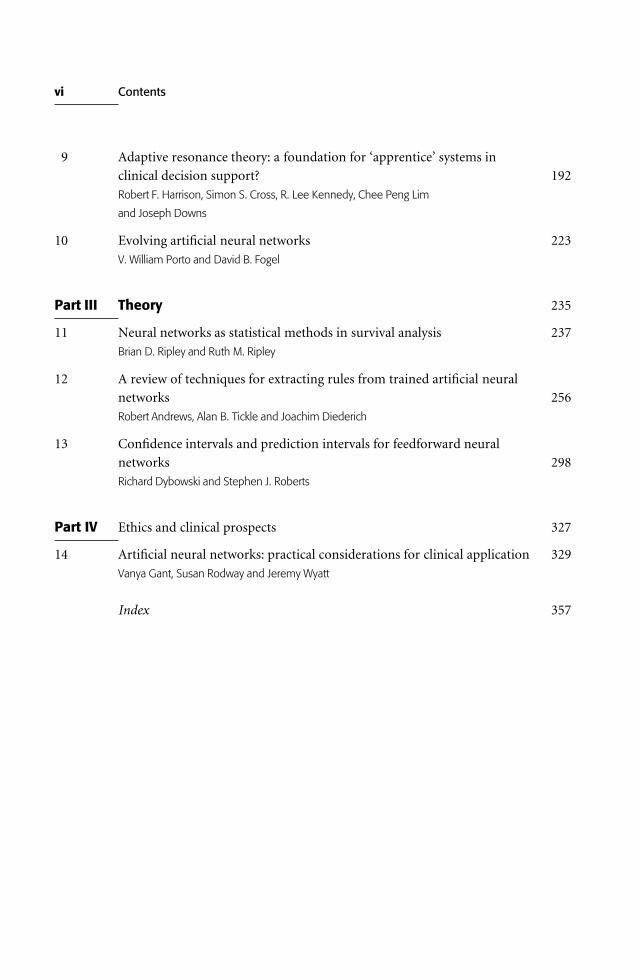
9 Adaptive resonance theory: a foundation for ‘apprentice’ systems in

clinical decision support? 192

Robert F. Harrison, Simon S. Cross, R. Lee Kennedy, Chee Peng Lim

and Joseph Downs

10 Evolving artiWcial neural networks 223

V. William Porto and David B. Fogel

Part III Theory 235

11 Neural networks as statistical methods in survival analysis 237

Brian D. Ripley and Ruth M. Ripley

12 A review of techniques for extracting rules from trained artiWcial neuralnetworks 256

Robert Andrews, Alan B. Tickle and Joachim Diederich

13 ConWdence intervals and prediction intervals for feedforward neural

networks 298

Richard Dybowski and Stephen J. Roberts

Part IV 327Ethics and clinical prospects

14 ArtiWcial neural networks: practical considerations for clinical application 329

Vanya Gant, Susan Rodway and Jeremy Wyatt

Index 357

vi Contents

1

1

Introduction

Richard Dybowski and Vanya Gant

In this introduction we outline the types of neural network featured in this book

and how they relate to standard statistical methods. We also examine the issue of

the so-called ‘black-box’ aspect of neural network and consider some possiblefuture directions in the context of clinical medicine. Finally, we overview the

remaining chapters.

A few evolutionary branches

The structure of the brain as a complex network of multiply connected cells(neural networks) was recognized in the late 19th century, primarily through the

work of the Italian cytologist Golgi and the Spanish histologist Ramon y Cajal.1

Within the reductionist approach to cognition (Churchland 1986), there appearedthe question of how cognitive function could be modelled by artiWcial versions of

these biological networks. This was the initial impetus for what has become a

diverse collection of computational techniques known as artiWcial neural networks(ANNs).

The design of artiWcial neural networks was originally motivated by the phe-

nomena of learning and recognition, and the desire to model these cognitiveprocesses. But, starting in the mid-1980s, a more pragmatic stance has emerged,

and ANNs are now regarded as non-standard statistical tools for pattern recogni-

tion. It must be emphasized that, in spite of their biological origins, they are not‘computers that think’, nor do they perform ‘brain-like’ computations.

The ‘evolution’ of artiWcial neural networks is divergent and has resulted in a

wide variety of ‘phyla’ and ‘genera’. Rather than examine the development of everybranch of the evolutionary tree, we focus on those associated with the types of

ANN mentioned in this book, namely multilayer perceptrons (Chapters 2–8,

10–13), radial basis function networks (Chapter 12), Kohonen feature maps(Chapters 2, 5), adaptive resonance theory networks (Chapters 2, 9), and neuro-

fuzzy networks (Chapters 10, 12).

We have not set out to provide a comprehensive tutorial on ANNs; instead, we

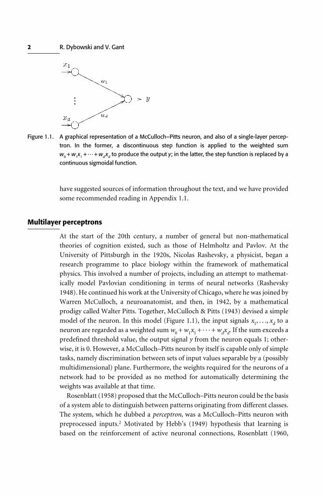
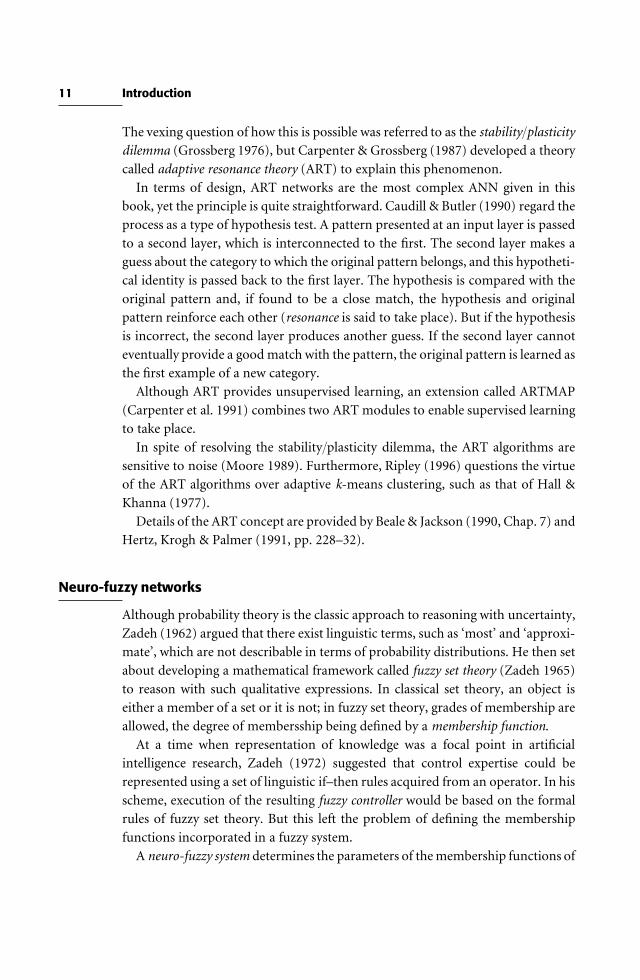
Figure 1.1. A graphical representation of a McCulloch–Pitts neuron, and also of a single-layer percep-tron. In the former, a discontinuous step function is applied to the weighted sumw0 + w1x1 + · · · + wd xd to produce the output y; in the latter, the step function is replaced by acontinuous sigmoidal function.

2 R. Dybowski and V. Gant

have suggested sources of information throughout the text, and we have provided

some recommended reading in Appendix 1.1.

Multilayer perceptrons

At the start of the 20th century, a number of general but non-mathematicaltheories of cognition existed, such as those of Helmholtz and Pavlov. At the

University of Pittsburgh in the 1920s, Nicolas Rashevsky, a physicist, began a

research programme to place biology within the framework of mathematicalphysics. This involved a number of projects, including an attempt to mathemat-

ically model Pavlovian conditioning in terms of neural networks (Rashevsky

1948). He continued his work at the University of Chicago, where he was joined byWarren McCulloch, a neuroanatomist, and then, in 1942, by a mathematical

prodigy called Walter Pitts. Together, McCulloch & Pitts (1943) devised a simple

model of the neuron. In this model (Figure 1.1), the input signals x1, . . ., xd to aneuron are regarded as a weighted sum w0 + w1x1 + · · · + wdxd. If the sum exceeds a

predeWned threshold value, the output signal y from the neuron equals 1; other-

wise, it is 0. However, a McCulloch–Pitts neuron by itself is capable only of simpletasks, namely discrimination between sets of input values separable by a (possibly

multidimensional) plane. Furthermore, the weights required for the neurons of a

network had to be provided as no method for automatically determining theweights was available at that time.

Rosenblatt (1958) proposed that the McCulloch–Pitts neuron could be the basis

of a system able to distinguish between patterns originating from diVerent classes.The system, which he dubbed a perceptron, was a McCulloch–Pitts neuron with

preprocessed inputs.2 Motivated by Hebb’s (1949) hypothesis that learning is

based on the reinforcement of active neuronal connections, Rosenblatt (1960,

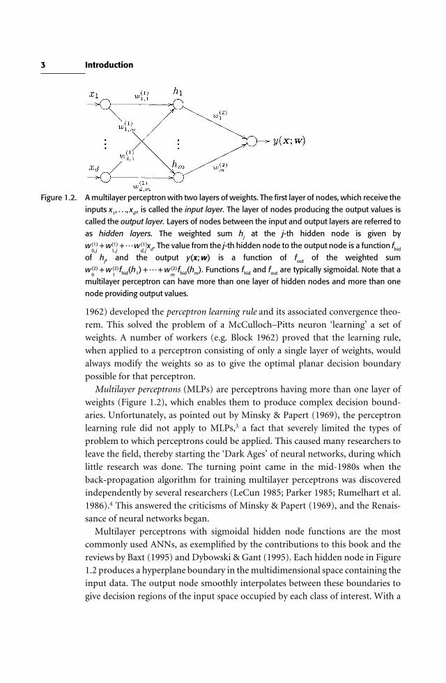
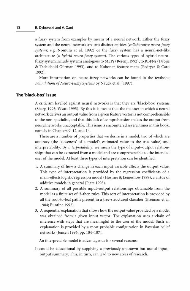
Figure 1.2. A multilayer perceptron with two layers of weights. The first layer of nodes, which receive theinputs x1, . . ., xd , is called the input layer. The layer of nodes producing the output values iscalled the output layer. Layers of nodes between the input and output layers are referred toas hidden layers. The weighted sum hj at the j-th hidden node is given byw(1)

0, j+ w(1)

1, j+ · · · w (1)

d, jxd. The value from the j-th hidden node to the output node is a function fhid

of hj, and the output y(x; w) is a function of fout of the weighted sumw(2)

0+ w (2)

1fhid(h1) + · · · + w (2)

mfhid(hm). Functions fhid and fout are typically sigmoidal. Note that a

multilayer perceptron can have more than one layer of hidden nodes and more than onenode providing output values.

3 Introduction

1962) developed the perceptron learning rule and its associated convergence theo-

rem. This solved the problem of a McCulloch–Pitts neuron ‘learning’ a set ofweights. A number of workers (e.g. Block 1962) proved that the learning rule,

when applied to a perceptron consisting of only a single layer of weights, would

always modify the weights so as to give the optimal planar decision boundarypossible for that perceptron.

Multilayer perceptrons (MLPs) are perceptrons having more than one layer of

weights (Figure 1.2), which enables them to produce complex decision bound-aries. Unfortunately, as pointed out by Minsky & Papert (1969), the perceptron

learning rule did not apply to MLPs,3 a fact that severely limited the types of

problem to which perceptrons could be applied. This caused many researchers toleave the Weld, thereby starting the ‘Dark Ages’ of neural networks, during which

little research was done. The turning point came in the mid-1980s when the

back-propagation algorithm for training multilayer perceptrons was discoveredindependently by several researchers (LeCun 1985; Parker 1985; Rumelhart et al.

1986).4 This answered the criticisms of Minsky & Papert (1969), and the Renais-

sance of neural networks began.Multilayer perceptrons with sigmoidal hidden node functions are the most

commonly used ANNs, as exempliWed by the contributions to this book and the

reviews by Baxt (1995) and Dybowski & Gant (1995). Each hidden node in Figure1.2 produces a hyperplane boundary in the multidimensional space containing the

input data. The output node smoothly interpolates between these boundaries to

give decision regions of the input space occupied by each class of interest. With a

4 R. Dybowski and V. Gant

single logistic output unit, MLPs can be viewed as a non-linear extension oflogistic regression, and, with two layers of weights, they can approximate any

continuous function (Blum & Li 1991).5 Although training an MLP by back-

propagation can be a slow process, there are faster alternatives such as Quickprop(Fahlman 1988).

A particularly eloquent discussion of MLPs is given by Bishop (1995, Chap. 4)

in his book Neural Networks for Pattern Recognition.

A statistical perspective on multilayer perceptrons

The genesis and renaissance of ANNs took place within various communities, and

articles published during this period reXect the disciplines involved: biology andcognition, statistical physics, and computer science. But it was not until the early

1990s that a probability-theoretic perspective emerged, with Bridle (1991), Ripley

(1993), Amari (1993) and Cheng & Titterington (1994) being amongst the Wrst toregard ANNs as being within the framework of statistics. The statistical aspect of

ANNs has also been highlighted in textbooks by Smith (1993), Bishop (1995) and

Ripley (1996).A recurring theme of this literature is that many ANNs are analogous to, or

identical with, existing statistical techniques. For example, a popular statistical

method for modelling the relationship between a binary response variable y and avector (an ordered set) of covariates x is logistic regression (Hosmer & Lemeshow

1989; Collett 1991), but consider the single-layer perceptron of Figure 1.1:

y(x; w) = foutAw0 +d

;i=1

wixiB . (1.1)

If the output function fout of Eq. (1.1) is logistic,

fout(r) = 1 + exp[ − (r)]−1,

(where r is any value) and the perceptron is trained by a cross-entropy error

function, Eq. (1.1) will be functionally identical with a main-eVects logisticregression model

p(y = 1 D x) =G1 + expC− (b0 +d

;i=1

bixi)DH−1

.

Using the notation of Figure 1.2, the MLP can be written as

y(x; w) = foutAw (2)0

+m

;j=1

w (2)j

fhidAw(1)0,j

+d

;i=1

w(1)i,j

xiBB , (1.2)

but Hwang et al. (1994) have indicated that Eq. (1.2) can be regarded as a

5 Introduction

particular type of projection pursuit regression model when fout is linear:

y(x; w) = v0 +m

;j=1

vj fjAu0,j +d

;i=1

ui,j xiB . (1.3)

Projection pursuit regression (Friedman & Stuetzle 1981) is an established statisticaltechnique and, in contrast to an MLP, each function fj in Eq. (1.3) can be diVerent,

thereby providing more Xexibility.6 However, Ripley and Ripley (Chapter 11)

point out that the statistical algorithms for Wtting projection pursuit regression arenot as eVective as those for Wtting MLPs.

Another parallel between neural and statistical models exists with regard to the

problem of overWtting. In using an MLP, the aim is to have the MLP generalizefrom the data rather than have it Wt to the data (overWtting). OverWtting can be

controlled for by adding a regularization function to the error term (Poggio et al.

1985). This additional term penalizes an MLP that is too Xexible. In statisticalregression the same concept exists in the form of the Akaike information criterion

(Akaike 1974). This is a linear combination of the deviance and the number of

independent parameters, the latter penalizing the former. Furthermore, whenregularization is implemented using weight decay (Hinton 1989), a common

approach, the modelling process is analogous to ridge regression (Montgomery &

Peck 1992, pp. 329–344) – a regression technique that can provide good generaliz-ation.

One may ask whether the apparent similarity between ANNs and existing

statistical methods means that ANNs are redundant within pattern recognition.One answer to this is given by Ripley (1996, p. 4):

The traditional methods of statistics and pattern recognition are either parametric based on afamily of models with a small number of parameters, or non-parametric in which the modelsused are totally flexible. One of the impacts of neural network methods on pattern recogni-tion has been to emphasize the need in large-scale practical problems for something inbetween, families of models with large but not unlimited flexibility given by a large number ofparameters. The two most widely used neural network architectures, multi-layer perceptronsand radial basis functions (RBFs), provide two such families (and several others already inexistence).

In other words, ANNs can act as semi-parametric classiWers, which are moreXexible than parametric methods (such as the quadratic discriminant function

(e.g. Krzanowski 1988)) but require fewer model parameters than non-parametric

methods (such as those based on kernel density estimation (Silverman 1986)).However, setting up a semi-parametric classiWer can be more computationally

intensive than using a parametric or non-parametric approach.

Another response is to point out that the widespread fascination for ANNs has

6 R. Dybowski and V. Gant

attracted many researchers and potential users into the realm of pattern recogni-tion. It is true that the neural-computing community rediscovered some statistical

concepts already in existence (Ripley 1996), but this inXux of participants has

created new ideas and reWned existing ones. These beneWts include the learning ofsequences by time delay and partial recurrence (Lang & Hinton 1988; Elman 1990)

and the creation of powerful visualization techniques, such as generative topo-

graphic mapping (Bishop et al. 1997). Thus the ANN movement has resulted instatisticians having available to them a collection of techniques to add to their

repertoire. Furthermore, the placement of ANNs within a statistical framework

has provided a Wrmer theoretical foundation for neural computation, and it hasled to new developments such as the Bayesian approach to ANNs (MacKay 1992).

Unfortunately, the rebirth of neural networks during the 1980s has been

accompanied by hyperbole and misconceptions that have led to neural networksbeing trained incorrectly. In response to this, Tarassenko (1995) highlighted three

areas where care is required in order to achieve reliable performance: Wrstly, there

must be suYcient data to enable a network to generalize eVectively; secondly,informative features must be extracted from the data for use as input to a network;

thirdly, balanced training sets should be used for underrepresented classes (or

novelty detection used when abnormalities are very rare (Tarassenko et al. 1995)).Tarassenko (1998) discussed these points in detail, and he stated:

It is easy to be carried away and begin to overestimate their capabilities. The usual conse-quence of this is, hopefully, no more serious than an embarrassing failure with concomitantmutterings about black boxes and excessive hype. Neural networks cannot solve everyproblem. Traditional methods may be better. Nevertheless, neural networks, when they areused wisely, usually perform at least as well as the most appropriate traditional method andin some cases significantly better.

It should also be emphasized that, even with correct training, an ANN will not

necessarily be the best choice for a classiWcation task in terms of accuracy. This hasbeen highlighted by Wyatt (1995), who wrote:

Neural net advocates claim accuracy as the major advantage. However, when a largeEuropean research project, StatLog, examined the accuracy of five ANN and 19 traditionalstatistical or decision-tree methods for classifying 22 sets of data, including three medicaldatasets [Michie et al. 1994], a neural technique was the most accurate in only one dataset,on DNA sequences. For 15 (68%) of the 22 sets, traditional statistical methods were the mostaccurate, and those 15 included all three medical datasets.

But one should add the comment made by Michie et al. (1994, p. 221) on the

results of the StatLog project:

With care, neural networks perform very well as measured by error rate. They seem to provideeither the best or near best predictive performance in nearly all cases . . .

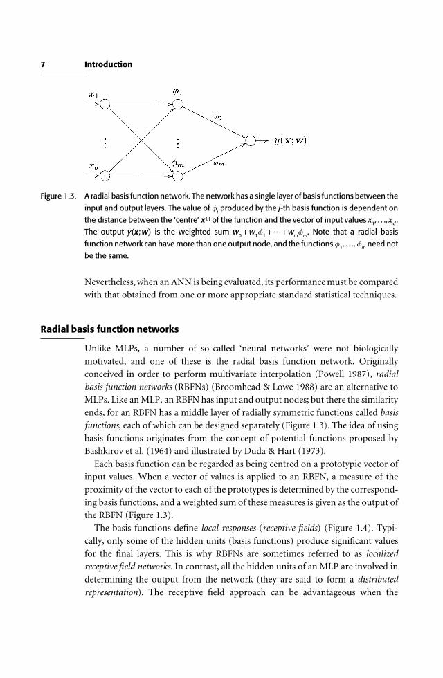
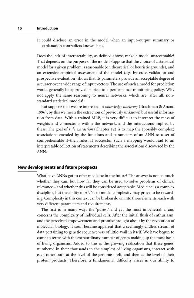
Figure 1.3. A radial basis function network. The network has a single layer of basis functions between theinput and output layers. The value of /j produced by the j-th basis function is dependent onthe distance between the ‘centre’ x [j] of the function and the vector of input values x1, . . ., xd .The output y(x; w) is the weighted sum w0 + w1/1 + · · · + wm/m. Note that a radial basisfunction network can have more than one output node, and the functions /1, . . ., /m need notbe the same.

7 Introduction

Nevertheless,when an ANN is being evaluated, its performance must be compared

with that obtained from one or more appropriate standard statistical techniques.

Radial basis function networks

Unlike MLPs, a number of so-called ‘neural networks’ were not biologically

motivated, and one of these is the radial basis function network. Originallyconceived in order to perform multivariate interpolation (Powell 1987), radial

basis function networks (RBFNs) (Broomhead & Lowe 1988) are an alternative to

MLPs. Like an MLP, an RBFN has input and output nodes; but there the similarityends, for an RBFN has a middle layer of radially symmetric functions called basis

functions, each of which can be designed separately (Figure 1.3). The idea of using

basis functions originates from the concept of potential functions proposed byBashkirov et al. (1964) and illustrated by Duda & Hart (1973).

Each basis function can be regarded as being centred on a prototypic vector of

input values. When a vector of values is applied to an RBFN, a measure of theproximity of the vector to each of the prototypes is determined by the correspond-

ing basis functions, and a weighted sum of these measures is given as the output of

the RBFN (Figure 1.3).The basis functions deWne local responses (receptive Welds) (Figure 1.4). Typi-

cally, only some of the hidden units (basis functions) produce signiWcant values

for the Wnal layers. This is why RBFNs are sometimes referred to as localizedreceptive Weld networks. In contrast, all the hidden units of an MLP are involved in

determining the output from the network (they are said to form a distributed

representation). The receptive Weld approach can be advantageous when the

Figure 1.4. Schematic representation of possible decision regions created by (a) the hyperplanes of amultilayer perceptron, and (b) the kernel functions of a radial basis function network. Thecircles and crosses represent data points from two respective classes.

8 R. Dybowski and V. Gant

distribution of the data in the space of input values is multimodal (Wilkins et al.

1994). Furthermore, RBFNs can be trained more quickly than MLPs (Moody &Darken 1989), but the number of basis functions required can grow exponentially

with the number of input nodes (Hartman et al. 1990), and an increase in the

number of basis functions increases the time taken, and amount of data required,to train an RBFN adequately.

Under certain conditions (White 1989; Lowe & Webb 1991; Nabney 1999), an

RBFN can act as a classiWer. An advantage of the local nature of RBFNs comparedwith MLP classiWers is that a new set of input values that falls outside all the

localized receptor Welds could be Xagged as not belonging to any of the classes

represented. In other words, the set of input values is novel. This is a morecautious approach than the resolute classiWcation that can occur with MLPs, in

which a set of input values is always assigned to a class, irrespective of the values.

For further details on RBFNs, see Bishop (1995, Chap. 5).

A statistical perspective on radial basis function networks

A simple linear discriminant function (Hand 1981, Chap. 4) has the form

g(x) = w0 +d

;i=1

wixi. (1.4)

with x assigned to a class of interest if g(x) is greater than a predeWned constant.This provides a planar decision surface and is functionally equivalent to the

McCulloch–Pitts neuron. Equation (1.4) can be generalized to a linear function of

functions, namely a generalized linear discriminant function

g(x) = w0 +m

;i=1

wi f (x), (1.5)

9 Introduction

which permits the construction of non-linear decision surfaces. If we represent anRBFN by the expression

g(x) = w0 +m

;i=1

wi/i( E x − x[i] E ), (1.6)

where E x − x[i] E denotes the distance (usually Euclidean) between input vector xand the ‘centre’ x[i] of the i-th basis function /i, comparison of Eq. (1.5) with Eq.(1.6) shows that an RBFN can be regarded as a type of generalized linear

discriminant function.

Multilayer perceptrons and RBFNs are trained by supervised learning. Thismeans that an ANN is presented with a set of examples, each example being a pair

(x, t), where x is a vector of input values for the ANN, and t is the corresponding

target value, for example a label denoting the class to which x belongs. The trainingalgorithm adjusts the parameters of the ANN so as to minimize the discrepancy

between the target values and the outputs produced by the network.

In contrast to MLPs and RBFNs,the ANNs in the next two sections are based onunsupervised learning. In unsupervised learning, there are no target values avail-

able, only input values, and the ANN attempts to categorize the inputs into classes.

This is usually done by some form of clustering operation.

Kohonen feature maps

Many parts of the brain are organized in such a way that diVerent sensory inputs

are mapped to spatially localized regions within the brain. Furthermore, theseregions are represented by topologically ordered maps. This means that the greater

the similarity between two stimuli, the closer the location of their corresponding

excitation regions. For example, visual, tactile and auditory stimuli are mappedonto diVerent areas of the cerebral cortex in a topologically ordered manner

(Hubel & Wiesel 1977; Kaas et al. 1983; Suga 1985). Kohonen (1982) was one of a

group of people (others include Willshaw & von der Malsburg (1976)) whodevised computational models of this phenomenon.

The aim of Kohonen’s (1982) self-organizing feature maps (SOFMs) is to map an

input vector to one of a set of neurons arranged in a lattice, and to do so in such away that positions in input space are topologically ordered with locations on the

lattice. This is done using a training set of input vectors n(1), . . ., n(m) and a set of

prototype vectors w(1), . . ., w(n) in input space. Each prototype vector w(i) isassociated with a location S(i) on (typically) a lattice (Figure 1.5).

As the SOFM algorithm presents each input vector n to the set of prototype

vectors, the vector w(i*) nearest to n is moved towards n according to a learning

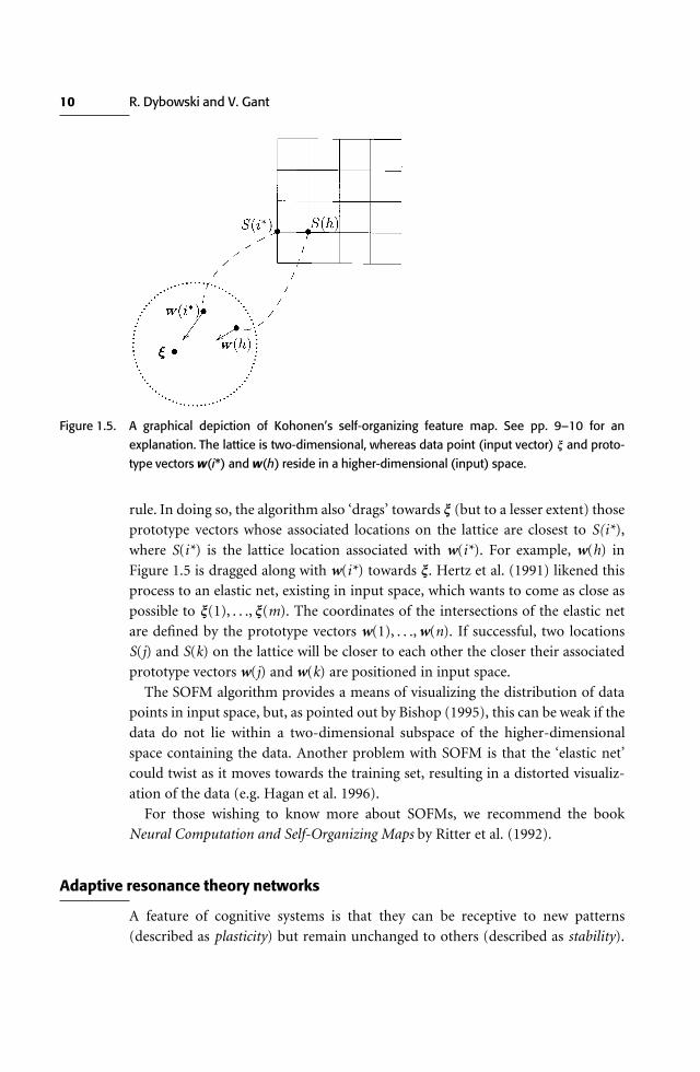
Figure 1.5. A graphical depiction of Kohonen’s self-organizing feature map. See pp. 9–10 for anexplanation. The lattice is two-dimensional, whereas data point (input vector) n and proto-type vectors w(i*) and w(h) reside in a higher-dimensional (input) space.

10 R. Dybowski and V. Gant

rule. In doing so, the algorithm also ‘drags’ towards n (but to a lesser extent) thoseprototype vectors whose associated locations on the lattice are closest to S(i*),

where S(i*) is the lattice location associated with w(i*). For example, w(h) in

Figure 1.5 is dragged along with w(i*) towards n. Hertz et al. (1991) likened thisprocess to an elastic net, existing in input space, which wants to come as close as

possible to n(1), . . ., n(m). The coordinates of the intersections of the elastic net

are deWned by the prototype vectors w(1), . . ., w(n). If successful, two locationsS(j) and S(k) on the lattice will be closer to each other the closer their associated

prototype vectors w(j) and w(k) are positioned in input space.

The SOFM algorithm provides a means of visualizing the distribution of datapoints in input space, but, as pointed out by Bishop (1995), this can be weak if the

data do not lie within a two-dimensional subspace of the higher-dimensional

space containing the data. Another problem with SOFM is that the ‘elastic net’could twist as it moves towards the training set, resulting in a distorted visualiz-

ation of the data (e.g. Hagan et al. 1996).

For those wishing to know more about SOFMs, we recommend the bookNeural Computation and Self-Organizing Maps by Ritter et al. (1992).

Adaptive resonance theory networks

A feature of cognitive systems is that they can be receptive to new patterns

(described as plasticity) but remain unchanged to others (described as stability).

11 Introduction

The vexing question of how this is possible was referred to as the stability/plasticitydilemma (Grossberg 1976), but Carpenter & Grossberg (1987) developed a theory

called adaptive resonance theory (ART) to explain this phenomenon.

In terms of design, ART networks are the most complex ANN given in thisbook, yet the principle is quite straightforward. Caudill & Butler (1990) regard the

process as a type of hypothesis test. A pattern presented at an input layer is passed

to a second layer, which is interconnected to the Wrst. The second layer makes aguess about the category to which the original pattern belongs, and this hypotheti-

cal identity is passed back to the Wrst layer. The hypothesis is compared with the

original pattern and, if found to be a close match, the hypothesis and originalpattern reinforce each other (resonance is said to take place). But if the hypothesis

is incorrect, the second layer produces another guess. If the second layer cannot

eventually provide a good match with the pattern, the original pattern is learned asthe Wrst example of a new category.

Although ART provides unsupervised learning, an extension called ARTMAP

(Carpenter et al. 1991) combines two ART modules to enable supervised learningto take place.

In spite of resolving the stability/plasticity dilemma, the ART algorithms are

sensitive to noise (Moore 1989). Furthermore, Ripley (1996) questions the virtueof the ART algorithms over adaptive k-means clustering, such as that of Hall &

Khanna (1977).

Details of the ART concept are provided by Beale & Jackson (1990, Chap. 7) andHertz, Krogh & Palmer (1991, pp. 228–32).

Neuro-fuzzy networks

Although probability theory is the classic approach to reasoning with uncertainty,

Zadeh (1962) argued that there exist linguistic terms, such as ‘most’ and ‘approxi-mate’, which are not describable in terms of probability distributions. He then set

about developing a mathematical framework called fuzzy set theory (Zadeh 1965)

to reason with such qualitative expressions. In classical set theory, an object iseither a member of a set or it is not; in fuzzy set theory, grades of membership are

allowed, the degree of membersship being deWned by a membership function.

At a time when representation of knowledge was a focal point in artiWcialintelligence research, Zadeh (1972) suggested that control expertise could be

represented using a set of linguistic if–then rules acquired from an operator. In his

scheme, execution of the resulting fuzzy controller would be based on the formalrules of fuzzy set theory. But this left the problem of deWning the membership

functions incorporated in a fuzzy system.

A neuro-fuzzy system determines the parameters of the membership functions of

12 R. Dybowski and V. Gant

a fuzzy system from examples by means of a neural network. Either the fuzzysystem and the neural network are two distinct entities (collaborative neuro-fuzzy

systems; e.g. Nomura et al. 1992) or the fuzzy system has a neural-net-like

architecture (a hybrid neuro-fuzzy system). The various types of hybrid neuro-fuzzy system include systems analogous to MLPs (Berenji 1992), to RBFNs (Dabija

& Tschichold-Gurman 1993), and to Kohonen feature maps (Pedrycz & Card

1992).More information on neuro-fuzzy networks can be found in the textbook

Foundations of Neuro-Fuzzy Systems by Nauck et al. (1997).

The ‘black-box’ issue

A criticism levelled against neural networks is that they are ‘black-box’ systems

(Sharp 1995; Wyatt 1995). By this it is meant that the manner in which a neuralnetwork derives an output value from a given feature vector is not comprehensible

to the non-specialist, and that this lack of comprehension makes the output from

neural networks unacceptable. This issue is encountered several times in this book,namely in Chapters 9, 12, and 14.

There are a number of properties that we desire in a model, two of which are

accuracy (the ‘closeness’ of a model’s estimated value to the true value) andinterpretability. By interpretability, we mean the type of input–output relation-

ships that can be extracted from a model and are comprehensible to the intended

user of the model. At least three types of interpretation can be identiWed:

1. A summary of how a change in each input variable aVects the output value.

This type of interpretation is provided by the regression coeYcients of amain-eVects logistic regression model (Hosmer & Lemeshow 1989), a virtue of

additive models in general (Plate 1998).

2. A summary of all possible input–output relationships obtainable from themodel as a Wnite set of if–then rules. This sort of interpretation is provided by

all the root-to-leaf paths present in a tree-structured classiWer (Breiman et al.

1984; Buntine 1992).3. A sequential explanation that shows how the output value provided by a model

was obtained from a given input vector. The explanation uses a chain of

inference with steps that are meaningful to the user of the model. Such anexplanation is provided by a most probable conWguration in Bayesian belief

networks (Jensen 1996, pp. 104–107).

An interpretable model is advantageous for several reasons:

It could be educational by supplying a previously unknown but useful input–

output summary. This, in turn, can lead to new areas of research.

13 Introduction

It could disclose an error in the model when an input–output summary orexplanation contradicts known facts.

Does the lack of interpretability, as deWned above, make a model unacceptable?

That depends on the purpose of the model. Suppose that the choice of a statisticalmodel for a given problem is reasonable (on theoretical or heuristic grounds), and

an extensive empirical assessment of the model (e.g. by cross-validation and

prospective evaluation) shows that its parameters provide an acceptable degree ofaccuracy over a wide range of input vectors. The use of such a model for prediction

would generally be approved, subject to a performance-monitoring policy. Why

not apply the same reasoning to neural networks, which are, after all, non-standard statistical models?

But suppose that we are interested in knowledge discovery (Brachman & Anand

1996); by this we mean the extraction of previously unknown but useful informa-tion from data. With a trained MLP, it is very diYcult to interpret the mass of

weights and connections within the network, and the interactions implied by

these. The goal of rule extraction (Chapter 12) is to map the (possibly complex)associations encoded by the functions and parameters of an ANN to a set of

comprehensible if–then rules. If successful, such a mapping would lead to an

interpretable collection of statements describing the associations discovered by theANN.

New developments and future prospects

What have ANNs got to oVer medicine in the future? The answer is not so muchwhether they can, but how far they can be used to solve problems of clinical

relevance – and whether this will be considered acceptable. Medicine is a complex

discipline, but the ability of ANNs to model complexity may prove to be reward-ing. Complexity in this context can be broken down into three elements, each with

very diVerent parameters and requirements.

The Wrst is in many ways the ‘purest’ and yet the most impenetrable, andconcerns the complexity of individual cells. After the initial Xush of enthusiasm,

and the perceived empowerment and promise brought about by the revolution of

molecular biology, it soon became apparent that a seemingly endless stream ofdata pertaining to genetic sequence was of little avail in itself. We have begun to

come to terms with the extraordinary number of genes making up the most basic

of living organisms. Added to this is the growing realization that these genes,numbered in their thousands in the simplest of living organisms, interact with

each other both at the level of the genome itself, and then at the level of their

protein products. Therefore, a fundamental diYculty arises in our ability to

14 R. Dybowski and V. Gant

understand such processes by ‘traditional’ methods. This tension has generatedamongst others the discipline of reverse genomics (Oliver 1997), which attempts

to impute function to individual genes with known and therefore penetrable

sequences in the context of seemingly impenetrable complex living organisms. Atthe time of writing, the potential of such mathematical methods to model these

interactions at the level of the single cell remains unexplored. ANNs may allow

complex biological systems to be modelled at a higher level, through thoughtfulexperimental design and novel data derived from increasingly sophisticated tech-

niques of physical measurement. Any behaviour at the single cell level productive-

ly modelled in this way may have fundamental consequences for medicine.The second level concerns individual disease states at the level of individual

human beings. The cause for many diseases continues to be ascribed (if not

understood) to the interaction between individuals and their environment. Oneexample here might be the variation in human response to infection with a

virulent pathogen, where one individual whose (genetically determined) immune

system has been programmed by his environment (Rook & Stanford 1998), maylive or die depending on how the immune system responds to the invader.

Complex data sets pertaining to genetic and environmental aspects in the life-or-

death interaction may be amenable to ANN modelling techniques. This questionof life or death after environmental insult has already been addressed using ANNs

in the ‘real’ context of outcome in intensive care medicine (e.g. Dybowski et al.

1996). We see no reason why such an approach cannot be extended to questions ofepidemiology. For example, genetic and environmental factors contributing to the

impressive worldwide variation in coronary heart disease continue to be identiWed

(Criqui & Ringel 1994), yet how these individual factors interact continues toelude us. An ANN approach to such formally unresolved questions, when coupled

with rule extraction (Chapter 12), may reveal the exact nature and extent of

risk-factor interaction.The third level concerns the analysis of clinical and laboratory observations and

disease. Until we have better tools to identify those molecular elements responsible

for the disease itself, we rely on features associated with them whose relationshipto disease remains unidentiWed and, at best, ‘second hand’. Examples in the real

world of clinical medicine include X-ray appearances suggestive of infection rather

than tumour (Medina et al. 1994), and abnormal histological reports of uncertainsigniWcance (PRISMATIC project management team 1999). Until the discipline of

pathology reveals the presence or absence of such abnormality at the molecular

level, many pathological Wndings continue to be couched in probabilistic terms;however, ANNs have the potential of modelling the complexity of the data at the

supramolecular level. We note some progress in at least two of these areas: the

screening of cytological specimens, and the interpretation of Xow-cytometric data.

15 Introduction

Clinical pathology laboratories are being subjected to an ever-increasing work-load. Much of the data received by these laboratories consists of complex Wgures,

such as cytological specimens – objects traditionally interpreted by experts – but

experts are a limited resource. The success of using ANNs to automate theinterpretation of such objects has been illustrated by the PAPNET screening

system (Chapter 3), and we expect that the analysis of complex images by ANNs

will increase with demand.We now switch to a diVerent channel in our crystal ball and consider three

relatively new branches on the evolutionary tree of neural computation, all of

which could have an impact on clinically oriented ANNs. The Wrst of these isBayesian neural computation, the second is support vector machines, and the

third is graphical models.

Bayesian neural computation

Whereas classical statistics attempts to draw inferences from data alone, Bayesian

statistics goes further by allowing data to modify prior beliefs (Lee 1997). This isdone through the Bayesian relationship

p(m D D) P p(m)p(D D m),

where p(m) is the prior probability of a statement m, and p(m D D) is the posterior

probability of m following the observation of data D. Another feature of Bayesianinference, and one of particular relevance to ANNs, is that unknown parameters

such as network weights w can be integrated out, for example

p(C D x, D) =Pw

p(C D x, w)p(w D D)dw,

where p(C D x, w) is the probability of class C given input x and weights w, and

p(w D D) is the posterior probability distribution of the weights.The Bayesian approach has been applied to various aspects of statistics (Gelman

et al. 1995), including ANNs (MacKay 1992). Advantages to neural computation

of the Bayesian framework include:

a principled approach to Wtting an ANN to data via regularization (Buntine &

Weigend 1991),

allowance for multiple solutions to the training of an MLP by a committee ofnetworks (Perrone & Cooper 1993),

automatic selection of features to be used as input to an MLP (automatic relevance

determination (Neal 1994; MacKay 1995)).

Bayesian ANNs have not yet found their way into general use, but, given their

16 R. Dybowski and V. Gant

capabilities, we expect them to take a prominent role in mainstream neuralcomputation.

Because of its intrinsic mathematical content, we will not give a detailed

account of the Bayesian approach to neural computation in this introduction;instead, we refer the interested reader to Bishop (1995, Chap. 10).

Support vector machines

Although the perceptron learning rule (see p. 3) is able to position a planardecision boundary between two linearly separable classes, the location of the

boundary may not be optimal as regards the classiWcation of future data points.

However, if a single-layer perceptron is trained with the iterative adatron algo-rithm (Anlauf & Biehl 1989), the resulting planar decision boundary will be

optimal.

It can be shown that the optimal position for a planar decision boundary is thatwhich maximizes the Euclidean distance between the boundary and the nearest

exemplars to the boundary from the two classes (the support vectors) (see e.g.

Vapnik 1995).One way of regarding an RBFN is as a system in which the basis functions

collectively map the space of input values to an auxiliary space (the feature space),

whereupon a single-layer perceptron is trained on points in feature space originat-ing from the training set. If the perceptron can be trained with a version of the

adatron algorithm suitable for points residing in feature space then the perceptron

will have been trained optimally. Such an iterative algorithm exists (the kerneladatron algorithm; Friess & Harrison 1998), and the resulting network is a support

vector machine. Vapnik (1995) derived a non-iterative algorithm for this optimiz-

ation task, and it is his algorithm that is usually associated with support vectormachines. A modiWcation of the procedure exists for when the points in feature

space are not linearly separable.

In order to maximize the linear separability of the points in feature space, a basisfunction is centred on each data point, but the resulting support vector machine

eVectively uses only those basis functions associated with the support vectors and

ignores the rest. Further details about support vector machines can be found in thebook by Cristianini & Shawe-Taylor (2000).

Neural networks as graphical models

Within mathematics and the mathematical sciences, it can happen that two

disciplines, developed separately, are brought together. We are witnessing thistype of union between ANNs and graphical models.

A (probabilistic) graphical model is a graphical representation (in the graph-

theoretic sense (Wilson 1985)) of the joint probability distribution p(X1, . . ., Xn)

17 Introduction

over a set of variables X1, . . ., Xn (Buntine 1994).7 Each node of the graph corre-sponds to a variable, and an edge between two nodes implies a probabilistic

dependence between the corresponding variables.

Because of their structure, graphical models lend themselves to modularity, inwhich a complex system is built from simpler parts. And through the theorems

developed for graphical models (Jensen 1996), sound probabilistic inferences can

be made with respect to the structure of a graphical model and its associatedprobabilities. Consequently, graphical models have been applied to a diversity of

clinical problems (see e.g. Kazi et al. 1998; Nikiforidis & Sakellaropoulos 1998). An

instructive example is the application of graphical models to the diagnosis of ‘blue’babies (Spiegelhalter et al. 1993).

The nodes of a graphical model can correspond to hidden variables as well as

to observable variables; thus MLPs (and RBFNs) can be regarded as directedgraphical models, for both have nodes, hidden and visible, linked by directed

edges (Neal 1992). An example of this is Bishop’s work on latent variable models,

which he has regarded from both neural network and graphical model viewpoints(Bishop et al. 1996; Bishop 1999). But graphical models are not conWned to the

layered structure of MLPs; therefore, the structure of a graphical model can, in

principle, provide a more accurate model of a joint probability distribution(Binder et al. 1997), and thus a more accurate probability model in those

situations where the variables dictate such a possibility.

In the 1970s and early 1980s, knowledge-based system were the focus of appliedartiWcial intelligence, but the so-called ‘knowledge-acquisition bottleneck’ shifted

the focus during the 1980s to methods, such as ANNs, in which knowledge could

be extracted directly from data. There is now interest in combining backgroundknowledge (theoretical and heuristical) with data, and graphical models provide a

suitable framework to enable this fusion to take place. Thus a uniWcation or

integration of ANNs with graphical models is a natural direction to explore.

Overview of the remaining chapters

This book covers a wide range of topics pertaining to artiWcial neural networks for

clinical medicine, and the remaining chapters are divided into four parts: I

Applications, II Prospects, III Theory and IV Ethics and Clinical Practice. The Wrstof these, Applications, is concerned with established or prototypic medical deci-

sion support systems that incorporate artiWcial neural networks. The section

begins with an article by Cross (Chapter 2), who provides an extensive review ofhow artiWcial neural networks have dealt with the explosion of information that

has taken place within clinical laboratories. This includes hepatological, radio-

logical and clinical-chemical applications, amongst others.

18 R. Dybowski and V. Gant

The PAPNET system for screening cervical carcinoma was one of the Wrst neuralcomputational systems developed for medical use. Boon and Kok (Chapter 3) give

an update on this system, and they do this from the viewpoints of the various

parties involved in the screening process, such as the patient, pathologist andgynaecologist.

QUESTAR is one of the most successful artiWcial neural network-based systems

developed for medicine, and Tarassenko et al. (Chapter 4) describe how QUES-TAR/BioSleep analyses the sleep of people with severe disorders such as obstruc-

tive sleep apnoea and Cheyne–Stokes respiration.

Chapter 5 by Braithwaite et al. describes Mary, a prototypic online systemdesigned to predict the onset of respiratory disorders in babies that have been born

prematurely. The authors have compared the performance of the multilayer

perceptron incorporated within Mary with that of a linear discriminant classiWer,and they also describe some preliminary Wndings based on Kohonen self-

organizing feature maps.

Niederberger and Golden (Chapter 6) describe another application based onmultilayerperceptrons,namely, the neUROnurological system.This predicts stone

recurrence following extracorporeal shock wave lithotripsy, a non-invasive pro-

cedure for the disruption and removal of renal stones. As with Chapter 5, theycompare theperformanceof theMLP with a lineardiscriminant classiWer.Theyalso

describe the useof Wilk’s generalized likelihood ratio test to elect which variables to

useas input for themultilayerperceptron.An interestingadjunct to theirwork is theavailability of a demonstration of neUROn via the World Wide Web.

This section closes with a review by Goodacre (Chapter 7) on the instrumental

approaches to the classiWcation of microorganisms and the use of multilayerperceptrons to interpret the resulting multivariate data. This work is a response to

the growing workload of clinical microbiology laboratories, and the need for rapid

and accurate identiWcation of microorganisms for clinical management purposes.In the section entitled Prospects, a number of feasibility studies are presented.

The Wrst of these is by Anderson and Peterson (Chapter 8), who provide a

description of how feedforward networks were used for the analysis of electroen-cephalograph waveforms. This includes a description of how independent compo-

nents analysis was used to address the problem of eye-blink contamination.

ARTMAP networks are one of the least-used ANN techniques. These networksprovide a form of rule extraction to complement the rule-extraction techniques

developed for multilayer perceptrons, and Harrison et al. (Chapter 9) describe

how ARTMAP and fuzzy ARTMAP can be used to automatically update aknowledge base over time. They do so in the context of the electrocardiograph

(ECG) diagnosis of myocardial infarction and the cytopathological diagnosis of

breast lesions.

19 Introduction

Like neural computation, evolutionary computation is an example of computerscience imitating nature. A solution given by Porto and Fogel (Chapter 10) to the

problem of Wnding a near-optimal structure for an artiWcial neural network is to

‘evolve’ a network through successive generations of candidate structures. Theyexplain how evolutionary computation has been used to design fuzzy min–max

networks that classify ECG waveforms and multilayer perceptrons that interpret

mammograms.The Wrst of the papers in the Theory section is by Ripley and Ripley (Chapter

11), who compare the performance of linear models of patient survival analysis

with their neural network counterparts. This is done with respect to breast cancerand melanoma survival data.

A response to the ‘black-box’ issue is to extract comprehensible sets of if–then

rules from artiWcial neural networks. Andrews et al. (Chapter 12) examine exten-sively how relationships between clinical attributes ‘discovered’ by ANNs can be

made explicit, thereby paving the way for hitherto unforeseen clinical insight, and

possibly providing a check on the clinical consistency of a network. They discussrule extraction with respect to MLPs, RBFNs, and neuro-fuzzy networks. Rule

extraction via fuzzy ARTMAP is also mentioned, and this chapter places the earlier

chapter by Harrison et al. in a wider context. The authors also look at rulereWnement, namely the use of ANNs to reWne if–then rules obtained by other

means.

By deWnition, some degree of uncertainty is always associated with predictions,and this includes those made by multilayer perceptrons. In the last chapter of this

section, Dybowski and Roberts review the various ways in which prediction

uncertainty can be conveyed through the use of conWdence and predictionintervals, both classical and Bayesian.

Finally, this book addresses some issues generated by combining these appar-

ently disparate disciplines of mathematics and clinical medicine. In the sectionentitled Ethics and clinical practice, Gant et al. (Chapter 14) present a critique on

the use of ‘black-box’ systems as decision aids within a clinical environment. They

also consider the ethical and legal conundrums arising out of the use of ANNs fordiagnostic or treatment decisions, and they address issues of which every practi-

tioner must be aware if they are to use neural networks in a clinical context.

NOTES

1. In the year that Golgi and Ramon y Cajal were jointly awarded the Nobel Prize for physiology

and medicine, Sherrington (1906) proposed the existence of special areas (synapses) where

neurons communicate, but it was not until the early 1950s (Hodgkin & Huxley 1952) that the

20 R. Dybowski and V. Gant

basic electrophysiology of neurons was understood.

2. The preprocessing was analogous to a hypothesis that the mammalian retina was composed

of receptive Welds. Each Weld was a limited area of the retina, the activation of which excited a

neuron associated with that Weld (Hubel & Wiesel 1962).

3. To avoid ambiguity, the number of layers of a perceptron should refer to the layers of

weights, and not to the layers of units (nodes), as this avoids a single-layer perceptron also

being regarded as a two-layer perceptron (Tarassenko 1998).

4. It was later found that the Wrst documented description of the back-propagation algorithm

was contained in the doctoral thesis of Werbos (1974).

5. With a single hidden layer, the number of hidden nodes required to approximate a given

function may be very large. If this is the case, a practical alternative is to insert an additional

hidden layer into the network.

6. Another non-linear statistical technique with Xexibility comparable to that of an MLP is

multivariate adaptive regression splines (Friedman 1991).

7. Graphical models are also known as belief networks, Bayesian networks and probabilistic

networks. Heckerman (1997) has written a good tutorial on this topic.

Appendix 1.1. Recommended reading

Recommending material to read is not easy. A suitable recommendation is dependent upon a

reader’s background knowledge, the topics on which he or she wants to focus, and the depth to

which he or she wishes to delve.

The only book of which we know that has attempted to introduce neural networks without

resorting to a single equation is that by Caudill & Butler (1990), with the unfortunate title of

Naturally Intelligent Systems. The book does manage to convey a number of concepts to a certain

extent; however, in order to learn more about neural computation, some mathematical literacy

is required. The basic tools of linear algebra, calculus, and probability theory are the prerequi-

sites, for which there are many suitable publications (e.g. Salas & Hille 1982; Anton 1984; Ross

1988).

The ideas encountered in Caudill & Butler’s (1990) Naturally Intelligent Systems (Chaps. 1–3,

8–10, 13, 14, 16) can be expanded upon by a visit to Beale & Jackson’s (1990) Neural Computing

(Chaps. 1–5, 8). Although somewhat mathematical, this book is by no means daunting and is

worthy of attention. After Beale & Jackson, the next step is undoubtedly Bishop’s (1995) Neural

Networks for Pattern Recognition, a clear and comprehensive treatment of a number of neural

networks, with an emphasis on their statistical properties – a landmark textbook.

For those wishing to go more deeply into the theory, there are a number of routes from which

to choose. These include taking a statistical perspective (e.g. Ripley 1996) and the statistical

physics approach (e.g. Hertz et al. 1991; Haykin 1994). On the other hand, those seeking

examples of medical applications can Wnd a diverse collection in the book ArtiWcial Neural

Networks in Biomedicine (Lisboa et al. 2000). We should also mention A Guide to Neural