Climatic variation and tree-ring structure in conifers: … · ayL '(9~61 s~ug) asuodsa~ s!$eurgs ql~ol6-aalJ ay1 6uwoys sauas aurg e uyqo 01 paAoural uaaq alzey sa6ueys al!s pue

Vol. 1: 97-116, 1991 l CLIMATE RESEARCH Clim. Res.

Published April 14

Climatic variation and tree-ring structure in conifers: empirical and mechanistic models of

tree-ring width, number of cells, cell size, cell-wall thickness and wood density

Harold C. ~ritts', Eugene A. Vaganov2, Irina V. sviderskaya2, Alexander V. shashkin2

' Laboratory of Tree-Ring Research, University of Arizona, Tucson. Arizona 85721, USA Laboratory of Wood Science and Dendrochronology, Institute of Forest and Wood, USSR Academy of Science,

Siberian Branch, Krasnoyarsk, USSR

ABSTRACT: Variations in tree-ring structure are simulated with (1) an empirical model using monthly climatic data as statistical predictors and (2) a mechanisbc model using daily climatic data as growth limiting conditions. The empirical model calibrates standardized ring-width and density chronologies of tree-rings with monthly temperature, precipitation or Palmer Drought Severity Index. The empirical model can be used with any tree-ring and climatic data set to evaluate linear, curvilinear or interactive relationships, to examine different types of calibration procedures, to calculate growth response to climatic factors, to compare the responses of different data sets, to examine a number of environmental questions about climatic change and to detect possible effects of altered environmental conditions on growth such as those caused by air pollution. The empirical model is applicable to any species and site where there is a tree-ring chronology and a climatic record of sufficient length. The mechanistic model uses mathematical equations to simulate processes affecting cell size, cell-wall thickness and wood density variations for individual rings using precipitation, temperature and humidity measurements. Limiting conditions are estimated from temperature, day length and a calculated water balance. The mechanistic model has been validated for Pinus sylvestris L. from dry sites in south Siberia and for P. ponderosa Laws. from southern Arizona. The results from both models are instructive as to what factors are important to the growth of different ring structures and when these factors become limiting. While the models will be developed further, they have already contnbuted to an understanding of tree-nng and climate relationships and have provided a number of answers to certain environmental questions. The empirical model is used in tandem with the mechanistic model to obain important insights on relationships that the mechanistic model calculations lack.

INTRODUCTION

Trees monitor environmental conditions that limit their biological processes, and this information is stored in the structure of the annual ring (Fritts 1976, Schweingruber 1988). Dendrochronology is a developing science dealing with annual and seasonal variations in tree-ring structures that have been precisely dated and arranged in annual time series (Fritts 1976, Schweingruber 1988).

Dendrochronological data are now recognized as important sources of information on (1) past, present

O Inter-Research/Printed in Germany

and future climatic changes (Fritts 1976, Hughes et al. 1982, Brubaker & Cook 1983, Briffa e t al. 1990, Cook & Kairiukstis 1990), (2) ecological changes in forest com- munities (Fritts & Swetnam 1989), (3) past geomorphic variations including earthquakes (Scuderi 1984, Jacoby et al. 1988), landslides (Schweingruber 1988) and volcanic activity (LaMarche & Hirschboeck 1984, Yama- guchi 1985, 1986, Baillie & Munro 1988, Scuderi 1990), and (4) a variety of geophysical questions, such as possible biotic effects of rising atmospheric CO2 (LaMarche e t al. 1986, Kienast & Luxmoore 1988), isotopic variations (Pilcher 1990), large-scale global

98 Clim. Res. 1: 97-116, 1991

circulation patterns (Fritts in press), solar variability, (Stockton et al. 1985) and climatic change (Briffa et al. 1990, Fritts in press).

Dendrochronological data are now being systemati- cally collected and archived for many land areas of the world (Stockton et al. 1985), and modern and sophisti- cated statistical techniques (see Chapters 3. 4 and 5 in Cook & Kairiukstis 1990) are being used for their analysis. Yet many existing models of forest growth (Dixon et al. 1990, Graham et al. 1990) do not consider the information on climate growth relationships that could be obtained from dendrochronological analysis (Fritts 1990).

MODELING TREE-RING CLIMATE RELATIONSHIPS

Models are formal representations of ideas, concepts, principles or applications of a discipline. They may be simple statements and diagrams of relationships (Wil- son & Howard 1968, Fritts 1976), or they may be more complex representations of entire systems involving mathematical expressions and computer simulations (Gay 1989, Dixon et al. 1990, Graham et al. 1990, Stout et al. 1990). According to Jeffers (1988), 'The advan- tages of formal mathematical expressions as models are: (1) they are precise and abstract; (2) they transfer information in a logical way; and (3) they act as an unambiguous medium of communication.' Our paper describes 2 mathematical models, which can be used in tandem or separately to investigate relationships or to predict and evaluate alternative outcomes involving climatic conditions governing dated tree-ring structures.

These structures include earlywood, latewood and annual ring width, cell size, cell-wall thickness and density of the wood, all of which can vary markedly from year to year. Variations in all of these structures can be related to variations of physiological processes within the trees that govern division, enlargement and differentiation of growing cells in the xylem (Wilson 1964, Wilson & Howard 1968, Kozlowslu 1971, Fritts 1976, Kramer & Kozlowski 1979). The initial modeling efforts use dendroclimatological materials that have come from climate-stressed sites (Fritts 1976, Schwein- gruber 1988, Fritts & Guiot 1990, Vaganov 1990). Thus, we have included many dendroclimatic procedures and have emphasized relationships between growth and limiting environmental conditions that are linked to variations in macroclimate (Fritts 1976). Now we are expanding the model to include more forest processes and ecological relationships including competition and productivity of the site.

However, all simulated relationships are based upon:

(1) well-known physiological principles involving cambial growth described in a variety of works including Lyr et al. (1967), Kozlowski (1971), Running et al. (1975), Fritts (1976), and Kramer & Kozlowski (1979); (2) published data on growth rates, cell production and cell-size variations throughout the growing season (Oppenheimer 1945, Bannan 1955, Smith & Wilsie 1961, Larson 1963, Kramer 1964, Wilson 1964, Zahner et al. 1964, Whitmore & Zahner 1966, Zahner 1968, Skene 1969, Wodzicki 1971, Denne 1976, Thompson & Hinckley 1977, Ford et al. 1978, Berlyn 1982); and (3) results from our own experiments on seasonal growth and tree-ring structure (Fritts 1976, Vaganov et al. 1985, Vaganov 1990).

The model calculations begin with either monthly or daily climatic data. An empirical model, called PRE- CON (for PRECONditioning) uses multivariate techniques to calibrate monthly temperature, precipitation and Paimer Drought Severity indices, PDSI (Palmer 1965), with standardized annual ring measurements, such as total width, earlywood width, latewood width, maximum density and minimum density (Fritts 1976, 1982, 1990, Fritts & Swetnam 1989, Fritts & Guiot 1990). A mechanistic model, called TRACH (for the TRACHeidogram described by Vaganov 1987, 1990), reads daily temperature and precipitation measurements for each year and uses mathematical equations to translate this information into (1) a daily water balance, (2) factors limiting cell growth, (3) daily changes in cell size, wall thickness and density and, finally, (4) cell size, wall thickness and wood density of one radial file of cells in the xylem. The programs are written in ANSI standard FORTRAN and compiled under Ryan McFarland FORTRAN 2.4 to run under DOS (Ryan McFarland Corporation, PO Box 20045, Austin, TX 78720-0045, USA). Data for graphics are written in ASCII code for input to Graph-In-The-Box Analytic, New England Software, Greenwich Office Park # 3, Greenwich, CT 06831, USA.

PRECON: STATISTICAL ASSESSMENT OF FACTORS AFFECTING CHRONOLOGIES

OF ANNUAL RINGS

General description

Dendrochronologists have utilized multivariate regression models to evaluate tree-ring and climate relationships (Fritts 1976, Lofgren & Hunt 1982) such as:

K

? I = 1 X i , k P k + d + E , k = O

(1)

where xirk are k statistical predictors representing climatic variables for year i, which are used to estimate

we~6old l!xa JO s3!qde~6 )e yOOl 'elep aAeS 33

s~sA/eue U! /(lrl!q~xalj ~oj s~olle - salqe!Jeh 43~~s 'q h!~el!Lu!s 40 sqls!lels aleLu!lsg .e

sa!Jas awl) 04 q3i1~s JO aleduo3 'L (peppe 6yeq /o ssa3o~d U!) Jailg ueuley aleln3le3 .g

lapow 41~016 au!d uJaqlnos Ja!JD pue Jauyez asn 'S

UO!SS~J~~J JUWUO~UO~ led!ou!~d - uo!punJ asuodsa~ aieln3le3 'p

slua!3y~ao3 UO!SS~J~~J 6~!leln3le3aJ lnoql!~ saleu!asa aielncrle~~atl '6 ure~6old u!eu ol l!xa Jo/pue UO~SS~J~~J aleln3le3au '4

se!j!~eeu!l-uou sassasse - salqepeh luJolsueJ1 'a

g a~n6y aas - 4~016 alelnqe3a~ pue a6ue1.p 3!)ew!p a3npo~lul 'p

S a~n61~ aas - uo!le~q!le3 UO!SS~J~~J JOJ lelualu! au!g a6uey3 -3

Ienraju! aDuap!guos se6ueq~ - lahal- j a6ueq3 -q

slua!3g~ao3 aJow JO auo 40 sanleh a6ueq3 Al!~e~i!qy 'e

s!sAleue UO!SS~J~~J aqi a6ueq3 '2

slold ~a~e3s JO sayas awl 'slua!3!uao3 UO!SS~J~~J lold 'L

nN3W S3SAlVNV H3H10 aNV NOISS3HC33H

sasaqlodAq snouea Isal 01 paleIn3le2 aq up3 Alue11ur1s jo sx~sgels pue s!sA[eue 30 asodlnd ioj pa6ueq3xa aq ue3 sJas elep 'pale1ns1esai suo1ssai6ai pue apeur aq ue3 sabueq3 10 sadh any .ialI!j ueurpx e q&~ elep azh~eue pue (0661) lau9 v lauqez Aq rapour e 6u1sn ql~oi6 ale1nuIrs 'sdqsuog -ela1 uopunj asuodsai pue uo1ssa~6ai 'uoge1ai -103 aql 30 uorlelndtueur pup uoqeuymexa MOI~

'aleur~-[s U! suo~leuea qpw asuodsal ql~o16 aql alelq~les 'elep ~leur~p A~qluour pue 6u!~-aail peal Iaporu 1e2mdura aq1 u1 sainpa3oid .T '61j

nuau wau 01 03 C

sqs!le~s paielaJ pue slua!3!gao3 uo!lela~~o3 le yool 'Z slold ~aue3s JO sa!Jas aw!l 'suo!lela~~o3 lold 'C

nN3W NOllWl3tItI03

elep 3!1ew!(3 pue 6u!~-aa~l pauodwl 'p

S~!~O(OUOJ~~ yueg elea 6u!~-aa~l leuo!leuJaiul '6

elep ale~1.1113 'sa!60louo~q3 h~suap pue I.~~P!M-~U!J ueadOJn3 jo slas aaJql 'Z elep alew!l3 'sa!6olouo~y3 qlp!~-6~1~ ue3!~auv 4~0~ JO slas OM~ , L

:wo~j xapu! lenp!saJ/pJepuels se sauauamseau /(l~suap/ylp!~ QV~H aNv 13313s

qsea JO ssgs~lels al!s pue saureu aql 'Iapour aql dq pap!lzold asoyl uroq papaIas ale sa~rj d6o~ouo~ys JI

'(9~61 s$~ud) b601ouo~qs e palIes S! airs pue sapads ~epsgxed e uro~j palsaIIos saaq jo a~dures e WOJJ

sasuodsa~ pnuue asay1 jo anleh ueau ayL '(9~61 s~ug) asuodsa~ s!$eurgs ql~ol6-aalJ ay1 6uwoys sauas aurg e uyqo 01 paAoural uaaq alzey sa6ueys al!s pue a6e 01 anp 141~0~6 U! spuall 1enpe~6 ay] pue palep dnesr601ouo~qso1puap uaaq ahey sluaur -alnseauI 6uu ,pazd1eue aq ue~ IPUIJOJ plepuels s~ql u1 uauum ppo~ aql U! d601ouo~qs 6uu-aaq due snqL '(0661 ianea) yueg elea 6u~3 aall IeuogeulaluI aql JO ~eu~loj aql UI ualluM sa!6olouo~qs sllodur~ .IO

(1 '61g) Iapour ay1 dq papvold sapj uolj sa16olouolq~ 6uu-aarl z 10 1 speal Iapour ay1 '~03311d u1 palq -urasse uaaq alley suy11~061e ~es!~s!lels 30 dlaue~ v

'(8861 zlalon v uasnaa ueA '9861 ~~SSIA) asuodsa~ ql~016 U! uoge! -.IPA aurg 6urlen1~lza IOJ poqlau e se pa3npo~lu1 uaaq alzeq sla1pj ueurex 'dlluasa~ alom '(0661 s!lsynu~e>~

'8 Too3 '8861 laqnl6u!a~rlss 'E861 Too3 3 laTPqn18 '2861 'le la saq6n~ '9~61 sllug) asn aprM U! dpua~ -Ins sasg2eld pue sampasold 1e~r6o~ouo~q~o~puap hueu jo saseq aql ale slapou qsns urolj saleugsa Ies!Js!IelS '(E861 laqsI!d '8 A~JE) '2861 la lo!n3 '2861 uoPJo3 V sllud '0861 layeqnla '6~61 'P Ja sllud '8t6l 'Ie la laqnl6~1a~rls~ '9t61 'Pt61 '96961 'P6961 'L961 'Z961 sll~ld) SaIqeueA ~ols!pald 6~0UlE' sagueauqos aAIosaJ d~ay 01 uo!ssal6a1 Iestuoues pue srsd~eue ~uauoduos [edpuud asn (1~61) 're la sljug dq padola~ap slapour uogsunj lajsueq pue uo~punj asuodsaa .palapour aq ues (l) .b3 U! u~oqs UPql sd!qsuogela~ xalduros aJOW 'OS[v '(6~61 'S961 '[P

la sllug '9L61 'e6961 sl~u.~) yl~ol6 30 sluaualnseau lsairp pue sassaso~d ~es!60101sAyd 30 suoge611sa~u1 plag uo paseq araM uorlelaldla~ul qayl pue sd!qsuog -elal paurnsse ay1 jo urloj leauq 1elaua6 ay1 '(8861 slajjar) au!l aq ues suorsuaur~p ay$ JO auo pue 'A~sno -auelInurrs d~qsuo~~e~a~ e 30 suo~suaur~p jo laqurnu e a~oldxa ol s~s~ua~ss alqeua slapour aleuelz!llnpy

'(0661 lo!n3 '8 sllud 'S861 'le la UolTsolS 'c861 'le la saq6nH '9~61 s~lug) aleurgsa uo!ssa~6a~ aql uoq s[enp!sal ay1 ale '3 pue luelsuos e SI e 'slua!s -~jjaos uo!ssal6al aql ale -xapu~ qlpj~-Bup P ''A

66 ainlsnlls 6u!~-aa~l pue uogeuen s!1eu1g3 :.[P ia sllu,~

100 Clim. Res. 1. 97-116, 1991

Correlation menu

PRECON calculates the correlation coefficients between each monthly climatic variable and the selected chronology for the specified time interval and then runs a stepwise multiple regression analysis on the same data set (Fig. 1). The values of the correlation coefficients can be plotted (Fig. 2a) or displayed on the screen along with the maximum, minimum and standard deviations of the observations. Plots of the actual, estimated and residual time series produced by the regression also can be displayed (Fig. 3a) as well as scatter plots showing the observations of one variable plotted against the observations of 2 other variables along with 2 splines fit to the clouds of data points (Fig. 4 ) . Other options in the correlation menu can save the data or exit to the regression menu'.

After leaving the correlahon menu, the simple correlahons cannot be manipulated and the response profile of simple correlations cannot be plotted

J J A S O N D J F M A M J J

chronology are scrolled across the screen. Default answers are supplied with each query of the model to assist the user in making reasonable choices. The chronology is selected by entering the abbreviated site name and species code shown on the screen and choosing the type of chronology. For imported data, only the file name is needed along with the input format, if the default format is not appropriate.

The model prompts for the required input data, such as the interval to be studied (up to 100 yr), the climatic variables to be read, the months to be assembled, the state code and climatic division. Monthly PDSI values as well as temperature and precipitation are available on disk for the USA; only the latter 2 variables are b

0.08 available for Europe. If European data are requested,

% 0.06 the identification numbers, names and characteristics - of available climatic records are scrolled across the 2 0.04

screen. For Europe, a default climatic station is iden- ,z 0.02 0

tified for each chronology, but the user can select any E a, 0

climatic record by entering a different station identifi- 0

cation number. Cl -0.02 ImmPrec

Monthly data for 1 or 2 climatic variables can be -0.04 unmTemp 0 5 10 15

selected from the 24 continuous months starting with J J A S O N D J F M A M J J the January record 1% yr prior to growth and ending with the December record following growth. Tempera- ture and precipitation for 14 mo starting in July of the prior year and ending with August are the default C

0.4 choices. In the current version, if 2 variables are cho-

a, 0.3 Sen. the same months must be selected for both varia- ,,, bles and a maximum of 19 continuous months (a total of

F 0.1 38 mo) is allowed. 0,

0 -0 - - g -0.1

-0.2

0 5 10 15 J J A S O N D J F M A M J J 1 2 3 Lags

Month Prior growth

Fig. 2. Three representat~ons of the modeled growth response are applied to a 68 yr chronology of Pinus ponderosa from Walnut Canyon, Arizona, that was calibrated with monthly temperature and precipitation for Arizona Divlsion 7 for 14 mo beginning with July and ending wlth August, when ring width growth was 95 % complete (Fritts 1976). (a) Simple correlation coefficients (values to ? 0.24 are significant, p = 0.95) which show ring width to be inversely correlated with temperature and directly correlated with precipitation for all but the last August; (b) the 9 significant stepwise multiple regression coefficients, which are the minimum number of predictor variables explaining 75 O/O of the variance of ring-width index; and (c) response funct~on coefficients, obta~ned from regression with principal components of climate, that help resolve colinearities among the predictor data sets. 57 O/O of the ring- width variance is explained by chrnate and 21 % explained by prior growth (total 78 "h). Boot-strap methods had not been implemented when this plot was generated, so the confidence

level used to test the coefficients are lower than 0.95 '10

Fritts et al.: Climatic variation and tree-ring structure 101

' ' , I . . 1 1900 1920 1940 1960

Year

1 X a, z - 0 """Residual

----Estimate

- 1 1900 1920 1940 1960

Year

1). This menu is described in the following section. Also, option 3 is usually used with the change menu, so it will be described in that section.

Option 4 performs a response function analysis (Fritts et al. 1971, Fritts 1974, Guiot et al. 1982, Fritts & Wu 1986, Cook & Kairiukstis 1990) of the selected data sets, which uses principal component regression of climatic variables along with prior growth to help resolve co- lineanties between the monthly temperature and precipitation data sets (Fig. 2c). A boot-strap method, described in Fntts & Guiot (1990), was recently added with the help of J. Guiot. The boot-strap method uses Monte Carlo simulation techniques to estimate the standard errors of the response function weights, and thus provides a robust significance test. This change meets some recent criticisms of the response function approach (Cook & Kairiukstis 1990, Fritts 1990) and makes it a viable alternative to stepwise regression.

Two other alternatives to stepwise multiple regression analyses can be modeled. The first (option 5 ; Fig. 1) is a simple growth model described for southern pines (Pinus taeda L., P, echinata Mill., P. palustris Mill., and P. elliottj Engelm.) by Zahner & Grier (1989),

Fiq. 3. Time series modeled as in Fig. 2 except that tempera- which uses climatic impact factors with scalers that are tuie and PDSI values for 15 mo from July to ~ e ~ t e m b e r were multiplied with rnonthiy PDSI values to estimate ring- used to estimate the ring-width index. (a) Using stepwise width index (Fig. 3b), The original Zahner & Grier multiple regression as in Fig. 2, including 2 variables, with the estimate accounting for 64 % of the actual ring-width var- was designed in the iance; (b) using the Zahner & Grier growth model with the eastern USA. The PRECON implementation extends estimate accounting for 57 % of the actual ring-width var- the model to lower montane, upper montane, and sub- * . iance. A comparison of the residuals shows remarkable agree- alpine zones from the western USA, have pro- ment between the statistical assessment and the Zahner &

Grier simulation gressively shorter growing seasons with increasing altitude as shown in Table 1'.

The growing season ranges from 8 mo in the south to Regression and other analysis menu 4 mo in the subalpine zone, and the relative importance

of the monthly PDSI values in the simulation is pro- All significant stepwise regression coefficients can be

plotted in the same format as the correlation coefficients allowina one to make com~arisons between ' The addition of these 3 zones in the western USA applies the "

these 2 types of statistics ( ~ i ~ ~ , 1 & 2b). ~i~~ series and model to situations beyond those investigated by Zahner & Grier. Since their model was not designed or validated for

scatter plots can be created as in the menu' these 3 zones, any estimates for these western climatic zones Option 2 offers a submenu, called the change menu, should be used with extreme caution and full acknowledge- which is used to change the regression equation (Fig. ment of these limitations

Actual Index

-- Prec

-.Temp

Fig. 4 . Scatter plots of any variable against 2 other variables can be used to identify non-linearities and to detect the presence of outliers in the data sets. The same data are used as in Fig. 2 with actual ring- width index plotted against February temperature and precipitation. Both relationships appear h e a r

with no extreme values evident

102 Clim. Res. 1: 97-116, 1991

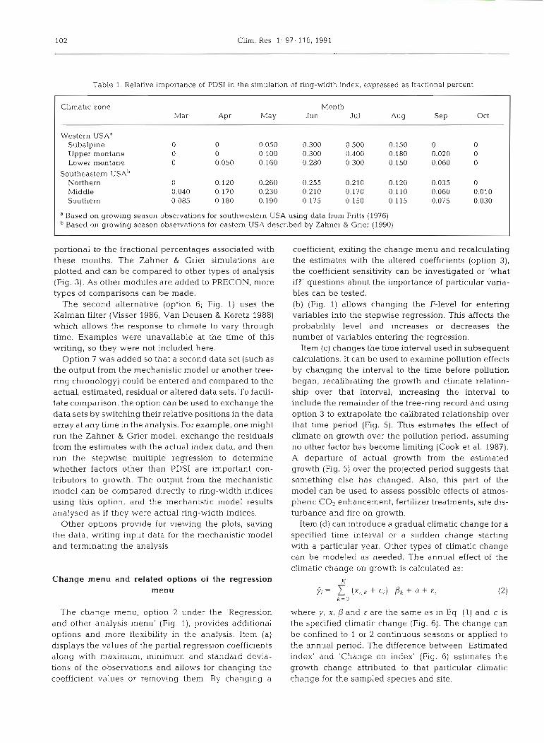
Table 1. Relative importance of PDSI in the simulation of ring-width index, expressed as fractional percent

Climatic zone Month Mar A P ~ May Jun Jul Aug S ~ P Oct

Western USA" Subalpine 0 0 0.050 0.300 0.500 0.150 0 0 Upper montane 0 0 0,100 0.300 0.400 0.180 0.020 0 Lower montane 0 0.050 0.160 0.280 0.300 0.150 0.060 0

Southeastern U S A ~ Northern 3 0.120 0.260 0.255 0.210 0.120 0.035 0 Middle 0.040 0.170 0.230 0.210 0.170 0.110 0.060 0.010 Southern 0.085 0.180 0.190 0.175 0.150 0.115 0.075 0.030

a Based on growing season observations for southwestern USA using data from Fritts (1976) Based on growing season observations for eastern USA described by Zahner & Grier (1990)

portional to the fractional percentages associated with these months. The Zahner & Grier simulations are plotted and can be compared to other types of analysis (Fig. 3). As other modules are added to PRECON, more types of comparisons can be made.

The second alternative (option 6; Fig. 1) uses the Kalman filter (Visser 1986, Van Deusen & Koretz 1988) which allows the response to climate to vary through time. Examples were unavailable at the time of this writing, so they were not included here.

Option 7 was added so that a second data set (such as the output from the mechanistic model or another tree- ring chronology) could be entered and compared to the actual, estimated, residual or altered data sets. To facilitate comparison, the option can be used to exchange the data sets by switching their relative positions in the data array at any time in the analysis. For example, one might run the Zahner & Grier model, exchange the residuals from the estimates with the actual index data, and then run the stepwise multiple regression to determine whether factors other than PDSI are important con- tributors to growth. The output from the mechanistic model can be compared directly to ring-width indices using this option, and the mechanistic model results analysed as if they were actual ring-width indices.

Other options provide for viewing the plots, saving the data, writing input data for the mechanistic model and terminating the analysis.

Change menu and related options of the regression menu

The change menu, option 2 under the 'Regression and other analysis menu' (Fig. l ) , provides additional options and more flexibility in the analysis. Item (a) displays the values of the partial regression coefficients along with maximum, minimum and standard deviations of the observations and allows for changing the coefficient values or removing them. By changing a

coefficient, exiting the change menu and recalculating the estimates with the altered coefficients (option 3), the coefficient sensitivity can be investigated or 'what if?' questions about the importance of particular variables can be tested. (b) (Fig. 1) allows changing the F-level for entering variables into the stepwise regression. This affects the probability level and increases or decreases the number of variables entering the regression.

Item (c) changes the time interval used in subsequent calculations. It can be used to examine pollution effects by changing the interval to the time before pollution began, recalibrating the growth and climate relationship over that interval, increasing the interval to include the remainder of the tree-ring record and using option 3 to extrapolate the calibrated relationship over that time period (Fig. 5). This estimates the effect of climate on growth over the pollution period, assuming no other factor has become limiting (Cook et al. 1987). A departure of actual growth from the estimated growth (Fig. 5) over the projected period suggests that something else has changed. Also, this part of the model can be used to assess possible effects of atmospheric CO2 enhancement, fertilizer treatments, site disturbance and fire on growth.

Item (d) can introduce a gradual climatic change for a specified time interval or a sudden change starting with a particular year. Other types of climatic change can be modeled as needed. The annual effect of the climatic change on growth is calculated as:

where y, X , p and E are the same as in Eq. (1) and c is the specified climatic change (Fig. 6). The change can be confined to 1 or 2 continuous seasons or applied to the annual period. The difference between 'Estimated index' and 'Change on index' (Fig. 6) estimates the growth change attributed to that particular climatic change for the sampled species and site.


Fig. 5. Item 2c in the 'Regression and other analysis menu' (Fig 1) allows cahbration over one time period (1896 to 1940) and extension of the calibration into another time period (1941 to 1984) to

X evaluate possible pollution effects on ring-width

Q) D index. Similar analyses include growth enhance- C - ... ... Residual ment from rising atmospheric CO2 or influences of

environmental or site factors on ring-width index .... ~ s t ~ m a t e Data are for Pinus ponderosa in the Santa Catalina

Mountains, north of Tucson, Arizona, where emis- C

. . . . -( - Actual sions after 1940 from distant copper smelters appear - l I n ' . n a I . . . I . . . I . ~ - . ' I

1900 1920 1940 1960 1980 Year

Fritts & Dean (unpubl.) applied the climatic change module to examine the hypothesis of Peterson (1988) that unusually low summer temperatures caused the prehistoric abandonment of Chaco Canyon, New Mex-

L 7

9 0 X Prec.

1 - - change a .- - Change o on ~ndex a,

6 0 Res~dual Index

", - 0

9. Temp.

? l change 3 - m - Change

on Index

Year

Fig. 6. Item 2e in the 'Regression and other analysis menu' (Fig. 1) can introduce a progressive or sudden climatic change and calculate its separate effect on the chronology ring-width index. Dashed-dot lines indicate the climatic change that was modeled, dashed lines are the estimates from climatic data (Fig. 3) and the heavy solid Lines are simulations with the hypothesized cllmatic change added to the relationship. The dfference between the dashed and heavy solid lines reflect the effect of climatic change on ring-width index. (a) Same data as in Fig. 2 but with a progressive decrease in percentage of precipitation simulated for 1930 to 1950; (b) data are for maximum density of Pinus sylvestris from Finland with temperatures hypothesized to rise by 0.04 "C yr-' during 1820 to

to have reduced growth. This possible pollution effect had not been recognized (Graybill & Rose 1989) until the PRECON empirical model was ap-

plied to the data set

ico. It was also well known that the widths of rings in trees growing during that time period decreased. Tree- ring chronologies growing in the same region were calibrated with 20th century temperature and precipitation records and then a decrease in summer temperature was modeled. Temperature was inversely related to ring width in all cases, and ring widths were modeled to increase, not decrease in response to a decline in temperature. It was concluded that summer temperatures during the time of abandonment were higher rather than lower and that high temperatures associated with drought, not low temperatures, were responsible for abandonment.

Grissino-Mayer & Fritts (in press) applied the change module to evaluate the future growth of a relict stand of Picea engelmanii growing on Mount Graham, Arizona, if greenhouse warming occurs as suggested by climatic models. Rising temperatures were simulated to increase ring widths in trees on a north-facing slope but to decrease ring widths in trees on a south-facing slope, where low soil moisture rather than low temperature is more likely to be limiting.

Fig. 6b is a similar analysis of a maximum density chronology from Pinus sylvestris, Pyhntunturi National Park, Finland. It examines the hypothesis of Briffa et al. (1990) that a regional greenhouse warming will not be detectable from Fennoscandia tree rings until 2020. A projected change of 0.04"C yr-' was simulated for 50 yr, and it increased maximum density by only 0.21 index units, which is only 1.29 standard deviations of the maximum density chronology. The small response is consistent with the Briffa et al. conclusions, but more than one chronology should be analyzed and other statistics examined, to make a thorough test of this hypothesis.

Item (e) (Fig. 1) can be selected to generate a variety of non-linear transformations, calculate interactions, combine several variables to obtain seasonal averaqes

1970 (see text for explanation). k n g width indices of Arizona and then make new ~h~ solves the P. ponderosa may be substantially reduced by relatively small deficits of annual precipitation, but maxlmum density indices equations showing significant curvilinear interactions

from P. sylvestris in Pyhntuntun National Park, Finland, and displays 3-dinlensional relationships as shown in appear less responsive to a 2 "C temperature rise Fig. 7

104 Clim. Res. 1: 97-116, 1991

Departure in winter prec~p~tation (Inches)

Fig. 7. Significant interactions and curvilinear relationships can be modeled and plotted. The equation for each interaction was solved by varying one variable at a hme over units of one standard deviation. This interaction between winter precipitation and temperature for August at the end of the growing season was found to be a significant predictor of ring width in Picea engelmanii growing at 3000 m on a south-facing slope of Mt. Graham. In this example, August temperature was held at -2 standard deviations (solid h e ) while precipitation values from -2 to +2 standard deviations were substituted into the equation and the resulting growth was plotted. The procedure was repeated for temperatures at - 1, 0, + l and +2 standard deviations (dashed and dotted lines). Low winter precipitation may be interpreted to be most growth-limiting when high August temperatures accentuate internal water stress. However, high winter moisture can also be growth-limiting through its effect on snow pack, delaying initiation ot growth, shortening growing season and reducing ring width. In the latter case, soil moisture reserves are adequate from high winter precipitation, so that low rather than high temperatures in August become growth-hiting by slowing down cell division, hastening the end of the growing season and contributing to reduced ring width. Such interactions and c u ~ h n e a r

relationships are important for accurate appraisal of climatic change effects

TRACH: MECHANISTIC SIMULATION OF RING STRUCTURE

Transformation of initial climatic data

Fritts (1976) presents schematic diagrams of a model relating variations in precipitation and temperature to variations in plant processes affecting ring-width. The mechanistic model (Fig. 8) is an attempt to replace this model with mathematical equations that govern these relationships. The modeling work began with the tracheidogram method of tree-ring analysis described by Vaganov (1990), which is concerned with cell size variations across the rings. The first version was a computer model developed by Vaganov et al. (1985), which uses daily climatic data to reconstruct cell size variations and related histometric properties of the annual ring.

In the current version, temperature is modeled as an important limiting factor through its effect on respira- tion and assimilative growth processes, as well as its effects on transpiration, evaporation from the soil and cell water stress (Kramer & Kozlowski 1979). Mean daily temperature measurements are used because they approximate the integrated effect of temperature variations over the day and also are standard meteorological measurements. Daily mean temperature data are converted to degrees Celsius and are used as model input without further transformation. Degree- day calculations are used to initiate cambial activity. Maximum, minimum, day and night temperatures and degree-day calculations will be used in future versions

of the model to characterize photosynthesis, respira- tion, damage from frosts and other growth-controlling factors.

Water storage in the soil and its availability throughout the season also regulates cambial activity and cell growth. Only a few direct measurements of water storage are available from meteorological records, and usually they are from stations far from forest sites. Measurements of precipitation are more widely available, but they do not portray the soil water dynamics that limit processes controlling growth. Thus, precipitation is converted to a soil-water balance using temperature and humidity deficit to calculate the daily evapotranspiration losses (Fig. 8).

The water balance (W,) for Day t is calculated as:

where W,-l = water balance on the previous day; P,-, = precipitation on Day t; k6 = coefficient of available precipitation (the portion of total daily precipitation that enters the soil); kg = coefficient of water loss from evapotranspiration; and F (TP-l,e,-l, W,-1) is a function that describes the water losses by evapotranspiration and depends upon temperature TP-l, air water deficit et-,, and water storage on the previous day.

The model calculations are:

where F (W,-1) is the S-shaped curve approximated by a third order polynomial that represents experimental data describing the dependence of evapotranspiration on soil moisture storage as shown in Kramer & Koz-

Fntts et a1 Climatic vanation and tree-rlng structure 105

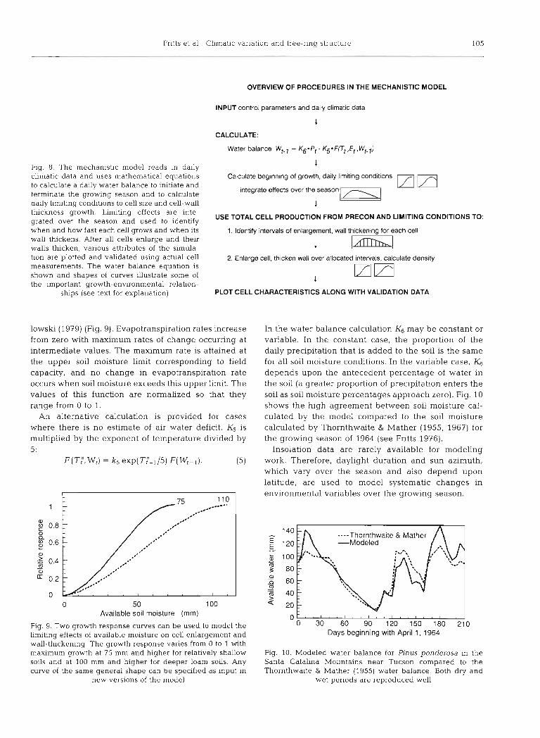
Fig. 8. The mechanistic model reads In daily climatic data and uses mathematical equations to calculate a dady water balance to Initlate and ternunate the growing season and to calculate daily limiting conditions to cell size and cell-wall thickness growth. Limiting effects are integrated over the season and used to identify when and how fast each cell grows and when its wall thickens. After all cells enlarge and then walls thicken, various attributes of the s~mula- tion are plotted and validated using actual cell measurements. The water balance equahon is shown and shapes of curves illustrate some of the important growth-environmental relation-

ships (see text for explanation)

OVERVIEW OF PROCEDURES IN THE MECHANISTIC MODEL

INPUT control parameters and dally climatic data

1

CALCULATE:

Water balance Wt-l + K6'Pt - K5'Frt ,Et, Wt-l)

Calculate beginning of growth, daily lhm~ting conditions

integrate effects over the season

1

USE TOTAL CELL PRODUCTION FROM PRECON AND LIMITING CONDITIONS TO:

1. Identify intervals of enlargement, wall thickening for each cell

2. Enlarge cell, thlcken wall over allocated intervals, calculate density

1

PLOT CELL CHARACTERISTICS ALONG WITH VALIDATION DATA

lowski (1979) (Fig. 9). Evapotranspiration rates increase from zero with maximum rates of change occurring at intermediate values. The maximum rate is attained at the upper soil moisture limit corresponding to field capacity, and no change in evapotranspiration rate occurs when soil moisture exceeds this upper limit. The values of this function are normalized so that they range from 0 to 1.

An alternative calculation is provided for cases where there is no estimate of air water deficit. Kg is multiplied by the exponent of temperature divided by 5:

F(TP,W,) = k5 exp(TP-,/5) F(W,-,l. (5)

0 0 50 100

Available soil molsture (mm)

Fig. 9. Two growth response curves can be used to model the limitlng effects of available moisture on cell enlargement and wall-thickening The growth response varies from 0 to 1 with maxlmum growth at 75 mm and higher for relatively shallow soils and at 100 mm and higher for deeper loam sods. Any curve of the same general shape can be specified as input in

new versions of the model

In the water balance calculation K6 may be constant or variable. In the constant case, the propornon of the daily precipitation that is added to the soil is the same for all soil moisture conditions. In the variable case, K6 depends upon the antecedent percentage of water in the soil (a greater proportion of precipitation enters the soil as soil moisture percentages approach zero). Fig. 10 shows the hlgh agreement between soil moisture calculated by the model compared to the soil moisture calculated by Thornthwaite & Mather (1955, 1967) for the growing season of 1964 (see Fntts 1976).

Insolation data are rarely available for modeling work. Therefore, daylight duration and sun azimuth, which vary over the season and also depend upon latitude, are used to model systematic changes in environmental variables over the growing season.

.---Thornthwa~te & Mather -Modeled

o - . , 1 ~ , ' , m ' 4 . ' , , 1 , , l , ,

0 30 60 90 120 150 180 210 Days beginning with April 1, 1964

Fig. 10. Modeled water balance for Pinus ponderosa in the Santa Catalina Mountains near Tucson compared to the Thomthwaite & Mather (1955) water balance. Both dry and

wet periods are reproduced well

Clim. Res. 1: 97-116, 1991

Growth-rate calculations

Temperature growth response. The temperature- dependent growth rate is modeled from experimental data summarized by Lyr et al. (1967), Fritts (1976) and Kramer & Kozlowski (1979) using 3 third-order polynomial curves with optimum responses at 12, 18 and 22 "C (Fig. 11).

The temperature response curves have the following characteristics: - for temperatures TP < 5 "C the growth response V (To) = 0, - for temperatures 5 "C < To < T",,, the growth response increases non-linearly with a gradual increase at the beginning, a rapid increase in the middle range and a gradual increase near the optimum, - for To = T&, the growth response V (To) = 1.0, - for temperatures To > T:,, the growth response decreases at an increasing rate until it reaches zero (due to the limitation of higher than optimum temperatures).

Water growth response. Growth is modeled to depend on the absolute value of soil moisture storage (expressed as mm of water contained in a 50 cm soil layer) using an S-shaped curve with field capacity at V,,, = 1.0 (Fig. 9). The dependence for soil moisture is approximated by the same third-order polynomial used to estimate the water budget F(W,-,). A different polynomial could be used if experimental data warrant it.

The soil moisture response curves have the following characteristics: - if W, = 0, the growth response V(W,) = 0 (a threshold moisture, Wmi,, can also be selected so that if W, < W,,, the growth response is zero), - if Wt > Wmi, the growth response V( W,) increases to a maximum value of 1.0 at the upper water limit, W4 - if W, > W4, growth is unlimited so V (W,) is 1.0.

Temperature (OC)

Fig. 11. Three growth response curves are used to model the limiting effects of average daily temperature on cell enlargement and wall-thickening. The growth response varies from 0 to 1 with maximum growth at 12, 18 and 22 "C Any curve of the same general shape can be specified as input in new

versions of the model

Now, a downward trend can be used to represent poorly drained conditions when W, > W4 if field measurements warrant it. In the present model, the trees are assumed to be growing on well-drained sites where excessive moisture is not commonly Limiting to growth.

Originally, variants with 2 different upper limits of the water growth response were available (Fig. 9). The upper limit, W4, was set at either 70 or l l 0 mm to allow for relatively loamy soils with a small or large range of available moisture. Now, the shapes of these curves can be specified by varying input variables.

Day length response. This parameter is used as an indirect representation of potential photosynthesis resulting from changes in day length, as well as the potential effects of day length on phenological behavior. The assumed growth response to day length V(L3 is linear:

where p and s are empirical coefficients depending on latitude and tree species. In simulations for Pinus syl- vesfris L, from dry sites in south Siberia, we used values of day length in hours, and for P. ponderosa Laws. from southern Arizona we used values of day length in relative units from tables of Thornthwaite & Mather (1967). These data are now generated from the latitude of the site using physical equations.

The day-length response has the following characteristics: for the longest day in the year, June 22, V(Lt) = 1.0; and for the equinox, September 22, V(L,) = 0.0 (in some cases a limiting day length of 13 rather than 12 h might be more appropriate).

Sun angle varies with latitude so the following equation was added and could be substituted for Eq. (6):

V(L,) = p cos0 (L, - z) (7)

where cos@ represents the highest sun angle at a given latitude for Day t. The limitmg effects of day length can be scaled upward or downward by specifying a scaling factor, with 1.0 corresponding to no scale change from the above computations.

Common growth response. Finally, 3 different growth responses, V, (To), V, (W) and V, (L) are calculated for each day. The tree growth response is calculated in 2 ways. A multiplicative growth model is calculated as:

A limited model is calculated as:

The multiplicative model includes the effects of each environmental factor in the common growth response while the limited model includes the effect of only that


factor that is most limiting. These results are expressed in units of relative growth ranging from 0 to 1.0.

Transforming growth rate curve to cell-size estimates

The calculated growth-rate array is transformed into a cell-size array (called a tracheidogram) by the following procedure' :

where Dj = cell size measured in the radial direction; = relative growth rate; Do = initial cell size, which is the size of the cambial daughter cell after division; and a = a scaler.

At first the curve V, is standardized for the duration of the growing period M2 - Ml. M, and M2 are input parameters of the program or l\gl may be estimated when the accumulation of a heat sum in degree-days starting with April 1 exceeds a specified value. Growth will not be calculated for days before the beginning date or after the end date even though environmental conditions may be favorable. The standardized tracheidogram is constructed for N cells as specified from program PRECON or entered by the user. If input from PRECON is requested, either the actual index, estimated index or index resulting from climatic change can be selected. An average radial dimension for cell size (ACS) of 20 pm (the value for Pinusponder- osa) is assumed unless the user enters a different value. At present an average ring width of 1000 pm is also assumed, but this parameter may also be programmed to change with the productivity of the site, tree age, crown class, stand stocking conditions or other factors affecting ring width.

Ring width (RW) is calculated as:

where I = the selected ring-width index value, and ARW = the average ring width.

The cell number is calculated as:

N = RW/ACS - 24.5 exp (- 0.005 RW) + 1 (12)

based on the relationship shown by Terskov et al. (1981).

The value of V, the integrated growth response, is obtained as:

M2 IVl, V2) V = (1IN) V,

t=M, (13)

The reverse procedure of converting cell-size measurements to growth-rate is described by Vaganov et al. (1985).

where the integral for V is the sum of M , - Ad2, the beginning and end of the growing season portioned out to the interval of favorable growing conditions assigned to the cell. Thus, each cell in the time sequence is formed during a period of 1 /N of the total integral. The calculations are made at time steps of 0.05 d and one cell is formed at time ( t ) , terminating whenever the consecutive summation equals a multiple of V corresponding to the transition to the next cell.

Cell size is calculated as in Eq. (10):

D, = Do + (RW- NDo)/VT, (14)

where Do -- 7.0 pm and T, is the time interval of cell j growth during which

and N

Cell-wall thickness calculations

Cell-wall thickness ( C m ) in the radial direction is calculated using the experimental relationship noted for Pinus sylvestris by Vaganov et al. (1985) (Fig. 12a). If the cell sizes range between Do (ca 2.0 pm) and some intermediate value, D,, CWT, is directly correlated with cell size (D,) as follows:

CWT, = 0.25 Dj

When cell sizes exceed D,, CWT, decreases with increasing D, in the following manner:

CWT, = 0.00722 exp (-0.134 DJ ( D , ) ~ . ' ~ ) . ( l ? )

This is a negative exponential relationship based upon measurements obtained from Pinus sylvestris from dry and wet sites in the southern part of the Krasnoyarsk region. Since D, is closely correlated with the number of cells in the ring (r = 0.74), it is evaluated using that number to obtain C m m , , for each yearly data set. CWT, is calculated from Eq. (16) if Dj I D,; otherwise it is calculated from Eq. (l?).

This relationship was modified to accommodate measurements from Pinus ponderosa (Fig. 12b) where small thin-walled earlywood cells were often associated with mid-season drought. A similar modification also may be applied to subarctic tree-rings where 'light latewood' appears to be associated with thin-walled latewood and a cold summer climate (Filion et al. 1986). In this mochfication, normal latewood for D, I D, has the same dependence as Eq. (16), and Eq. (l?) is used to estimate the maximum CWT, associated with D, for P. ponderosa. Under drought conditions early in the

108 Clirn. Res. 1. 97-116, 1991

I . .

10 20 30 40

Cel! diameter (pm)

10 20 30 40 0 Earlywood cells

Latewood cells Q False ring cells

Fig. 12. Cell-wall thickness plotted against cell diameter in the radial direction. (a) For Pinus sylvestris with wide rings from the southern part of the Krasnoyarsk regon, USSR (Vaganov et al. 1985); (b) for P. ponderosa with a 'false ring' in 1964 from southern Arizona (see Figs. 17 & 18); (c) theoretical description of cell-wall simulation for P. ponderosa, vanant 1 for normal earlywood and

latewood and variant 2 for P. ponderosa earlywood under drought conditions; and (d) simulated values for the 1964 season

season, C W , is less than this maximum value which is evaluated from the inverse of V, (Eqs. 8 and 9) but using a later time period from that used to calculate CSj. This delay in the C W r e s p o n s e averages 11 d for P. ponderosa but can be changed by the user. The delay represents the interval of time required for ma- turation (cell-wall thickening) to occur, and in this version of the model it is assumed to be constant over the entire growing season. This must b e changed to vary the interval over the growing season. More cell- wall thickness measurements are being collected to help refine this part of the model.

The following steps are used in the calculation: ( 1 ) Estimate the mean growth rate 7 ( t + 6 t ) for cell

enlargement where t is the day when cell enlargement is complete and 6 t is the time delay;

(2) Calculate the inverse value, 1.0 - 7 ( t + 6 t ) , so that favorable conditions for cell-wall thickening are estimated when conditions are unfavorable for cell enlargement and

(3) Calculate the real CWT, as:

where CWT,,, is the minimal value of CWT (ca 2.0 pm) and the terms to the right represent the different between the CWT estimated from Eqs. (16) and ( l?)

Density calculations

The 2 simulated cell characteristics, CS and CWT, are then used to obtain density estimates. Three assumptions are necessary to make the calculations:

( 1 ) The mean tangential diameter of the cells, D?, is relatively constant;

(2) DT is ca 30 pm ' . (3) The cell-wall thickness is the same on all sides of

the cross section. Density (optical density), DEN,, of each cell is calcu-

lated as:

DEN, = 1.0 - (D, - 2.0 CWT,) (DT - 2.0 CW,)/(DT D,

(19)

where D,, CWT, and DT are the same as defined above. The physical wood density, DEN,,,, can be estimated as:

DEN, = 1.5 DEN, (20)

where 1.5 is the density of wood substance. A wood density trace IS simulated by converting the x-axis from cell number to distance from the ring boundary. The data are automatically written to files that can be read by the graphics program, plotted on the screen or sent to the printer

and CWTmi, reduced in proporbon to soil moisture, This was the value obtained from 10 000 measurements of

temperature or light conditions that are limiting. Fig. 12 tangential diameters from sy,vestris growing on both shows the cell size and cell-wall thckness relationships dm and wet ,,te, south of Krasnoyarsk (Vaqanov et al. 1985) used in the model. and is reasonable for P. pondero;a.


Other TRACH features +Measured o Modeled

Other features of the TRACH model should be noted. The model is based on a relatively small number of parameters which may be changed or selected depending upon the conditions and species to be simulated. They are: - 3 temperature curves with different To,,; - base-level for calculating heat-sum; - total heat-sum to initiate growth; - the proportion of precipitation entering the soil, Kg,

which may or may not vary with soil moisture; - the coefficient of water loss, Kg (multiplier for evap-

oration) ; - initial soil moisture, WO; - 2 levels of maximum available soil moisture, W4,

where growth is optimum; - humidity deficit which may be read in or estimated; - a scaled day length value with or without azimuth; - beginning of growth which may be specified or cal-

culated from the total heat-sum; - end of growth; - cell numbers and ring width estimated from index

data in PRECON or specified by the user; - average cell size to model (not needed if width and

cell numbers are specified by the user); and - smooth growth or temperature data using an arith-

metic 7 d average, a one-sided (7 d) filter or a longer one-sided (12 d) filter. Different values must be assigned to these parame-

ters to model either limiting or enhancing environments for trees of different species or trees growing in different habitats. We selected default values to be the optimal parameters for Pinus ponderosa in southern Arizona. Independent water balance estimates, measured cell sizes and wall thicknesses are used to validate these results and tune the model. The means, mean squares and total mean squares of the differences between actual measurements and simulations are calculated and used in evaluating different input parameters.

Examples of TRACH model results on Pinus sylvestris

The first TRACH model was tested and tuned using climatic data and measurements from Pinus sylvesfn's growing in the southern Krasnoyarsk region of the USSR. All results were standardized to 30 cells to facilitate comparisons among rings of varying width. Daily climatic data from Bogard, 6 km from the trees, was used in the simulation. Analyses began with May 1, but the actual duration of the growing season was calculated as the continuous period of days for which the simulated growth rates were greater than zero. The

Cell number

Fig. 13. Comparison of measured and modeled radial cell- sizes for Pinus sylvestris from the southern part of the Kras-

noyarsk region, USSR, during different growing seasons

seasonal curves of temperature and air humidity dynamics were smoothed before analysis. The initial soil moisture was unknown, so 3 different values of initial soil moisture were used. All other conditions were the same. The initial values for the curves with the lowest root-mean-square deviation beetween the tracheidograms of the simulations and measurements were selected.

Fig. 13 includes the calculated and measured cell sizes from 6 rings formed during different growing seasons. The calculated data correlated well with the measured data both qualitatively and quantitatively. The simulated growing seasons began about May 15 and ended about August 15. From June 1 to July 15, 75 to 85 % of the cells in the ring were produced. Varia- tions in cell size later in the growing seasons appeared to be related to variations in soil moisture. Small cells in the latter half of the ring were associated with simulated drought, while large cells were associated with unusually moist conditions. In general, there is a rapid increase in growth at the beginning of the season followed by a progressive decline in growth associated with the transition from earlywood to latewood.

The simulations indicated that soil moisture storage at the beginning of the season plays a dominant role in determining cell-size variations throughout the annual ring. Thus, a realistic estimate of the water balance from precipitation and temperature is an important model consideration.

110 Clim. Res. 1. 97-116, 1991

0 High initial soil moisture

L o w initial soil moisture

Days in growlng season

L

10 20 30 Cell number

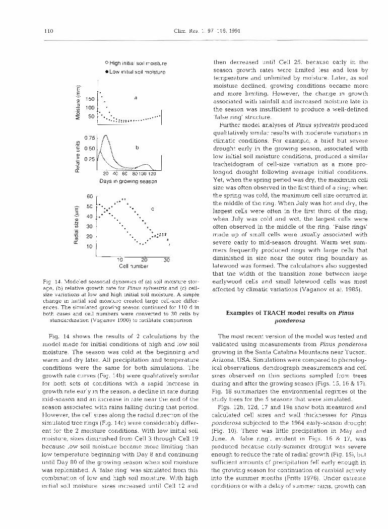
Fig. 14. Modeled seasonal dynamics of (a) soil moisture storage, (b) relative growth rate for Pinus sylvestris and (c) cell- size variations at low and high initial soil moisture. A simple change in initial soil moisture created large cell-size differences. The simulated growing season continued for 110 d in both cases and cell numbers were converted to 30 cells by

standardization (Vaganov 1990) to facilitate comparison

Fig. 14 shows the results of 2 calculations by the model made for initial conditions of high and low soil moisture. The season was cold at the beginning and warm and dry later. All precipitation and temperature conditions were the same for both simulations. The growth rate curves (Fig. 14b) were qualitatively similar for both sets of conditions with a rapid increase in growth rate early in the season, a decline in rate during mid-season and an increase in rate near the end of the season associated with rains falling during that period. However, the cell sizes along the radial direction of the simulated tree rings (Fig. 14c) were considerably dffer- ent for the 2 moisture conditions. With low initial soil moisture, sizes diminished from Cell 3 through Cell 19 because low soil moisture became more limiting than low temperature beginning with Day 8 and continuing until Day 80 of the growing season when soil moisture was replenished. A 'false ring' was simulated from this combination of low and high soil moisture. With high initial soil moisture, sizes increased until Cell 12 and

then decreased until Cell 25, because early in the season growth rates were limited less and less by temperature and unlimited by moisture. Later, as soil moisture declined, growing conditions became more and more Limiting. However, the change in growth associated with rainfall and increased moisture late in the season was insufficient to produce a well-defined 'false ring' structure.

Further model analyses of Pinus sylvestns produced qualitatively similar results with moderate variations in climatic conditions. For example, a brief but severe drought early in the growing season, associated with low initial soil moisture conditions, produced a similar tracheidogram of cell-size variation as a more pro- longed drought following average initial conditions. Yet, when the spring period was dry, the maximum cell size was often observed in the first third of a ring; when the spring was cold, the maximum cell size occurred in the middle of the ring. When July was hot and dry, the largest cells were often in the first third of the ring; when July was cold and wet, the largest cells were often observed in the middle of the ring. 'False rings' made up of small cells were usually associated with severe early to mid-season drought. Warm wet sum- mers frequently produced rings with large cells that diminished in slze near the outer ring boundary as latewood was formed. The calculations also suggested that the width of the transition zone between large earlywood cells and small latewood cells was most affected by climatic variations (Vaganov et al. 1985).

Examples of TRACH model results on Pinus ponderosa

The most recent version of the model was tested and validated using measurements from Pinus ponderosa growing in the Santa Catalina Mountains near Tucson, Arizona, USA. Simulations were compared to phenological observations, dendrograph measurements and cell sizes observed on thin sections sampled from trees during and after the growing season (Figs. 15, 16 & 17). Fig. 18 summarizes the environmental regimes of the study trees for the 5 seasons that were simulated.

Figs. 12b, 12d, 17 and 19a show both measured and calculated cell sizes and wall thicknesses for Pinus ponderosa subjected to the 1964 early-season drought (Fig. 10). There was little precipitation in May and June. A 'false ring', evident in Figs. 16 & l ? , was produced because early-summer drought was severe enough to reduce the rate of radal growth (Fig. 15), but sufficient amounts of precipitation fell early enough in the growing season for continuation of cambial activity into the summer months (Fritts 1976). Under extreme conditions or with a delay of summer rains, growth can

Fritts et al.: Climatic variation and tree-ring structure 11 1

l DENDROGRAPH C

DENDROGRAPH A

l - -

600 d

0 J F M A M J J A S O N D

Fig. 15. Daily maximum and minimum dendrographic measurements of stem size and phenological observations from one Pinus ponderosa for 1966 made at the base (Dendrograph A), middle (Dendrograph B) and upper (Dendrograph C) positions in the main stem, were used to check the growth that was simulated. T: apical buds swehng; B: buds opening; C: cambial activity initiated; N: needles emerging from bud; L: lignified latewood cells observed; M: needles reach mature size; t: days when the whole tree was enclosed in a plastic tent to obtain detailed physiological measurements (from Fritts

1976)

cease entirely so latewood cells that would have become a 'false ring' become true latewood and the cambium remains dormant unless a second growing period is initiated and a second ring is produced.

Daily climatic data collected at the tree sites (Fritts 1976, p. 97) (Fig. 18) were used in the simulation analysis. The estimated and actual measurements (Fig. 19a) are in good agreement. The mean square of the differences between the measured and modeledvalues were 10.8 for cell size and 0.447 for wall thickness, which are remark- ably acceptable errors for the analysis considering the dissimilarities noted between and within trees growing under the same climatic conditions.

During 1966, winter soil moisture was much higher and spring rain was absent, so soil moisture in spring steadily declined until late June when 50 mm of rain replenished some soil moisture. Bud opening was followed by the initiation of cambial activity in mid April and stems increased in size throughout May and June, but the rate of growth was reduced somewhat (Fig. 15) by the decline in soil moisture. High growth resumed after the June rain, but rates of growth decreased again as soil moisture became depleted (Fig. 18). When the summer rainy period began in mid July, growth rates rose again and remained normal until the end of the growing season. The 2 periods of growth reduction (Fig. 15) were associated with 2 troughs and peaks in both the cell size measurements and simulations (Fig. 19b), but the model placed the first trough and peak 2 to 3 cells too early. The simulations of cell size for 1966 did not agree

Cambium

Fig. 16. Photograph of cell-size variations from a basal section of a Pinus ponderosa stem used to validate the simulation

(from Fritts 1976)

112 Clim. Res. 1. 97-116, 1991

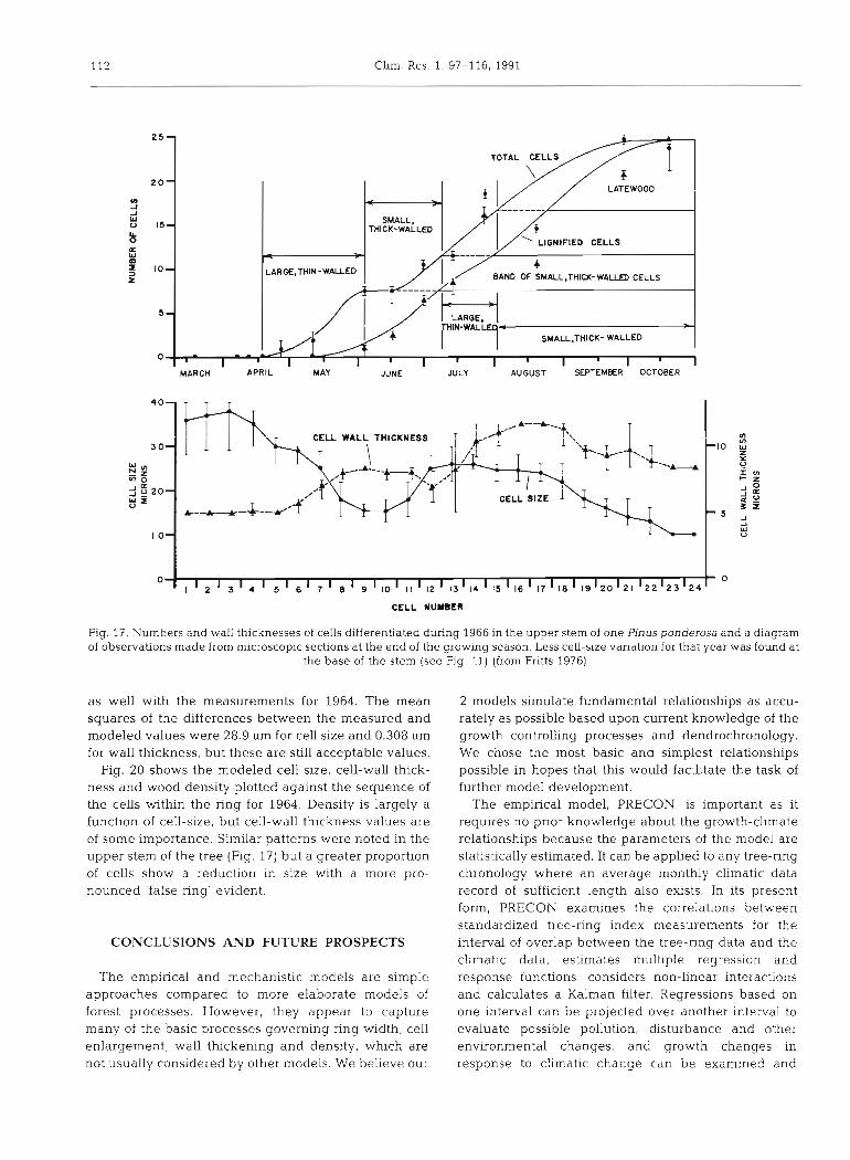
LATEWOOD

t

MARCH APRIL MAY JUNE JULY AUGUST SEPTEMBER OCTOBER

5-

1 WALL THICKMESS

T \ T

/p SMALL.THlCK- WALLED

.I 1 I CELL SIZE

0 ,- - m

1 I I I I I I I I I I I I 3

CELL NUMBER

Fig. 17. Numbers and wall thicknesses of cells differentiated during 1966 in the upper stem of one Pinus ponderosa and a diagram of observations made from microscopic sections at the end of the groulng season. Less cell-size vanation for that year was found at

the base of the stem (see Fig. 11) (from Fritts 1976)

as well with the measurements for 1964. The mean squares of the differences between the measured and modeled values were 28.9 pm for cell size and 0.308 pm for wall thickness, but these are still acceptable values.

Fig. 20 shows the modeled cell size, cell-wall thickness and wood density plotted against the sequence of the cells within the ring for 1964. Density is largely a function of cell-size, but celI-wall thickness values are of some importance. Similar patterns were noted in the upper stem of the tree (Fig. 17) but a greater proportion of cells show a reduction in size with a more pro- nounced 'false ring' evident.

CONCLUSIONS AND FUTURE PROSPECTS

The empirical and mechanistic models are simple approaches compared to more elaborate models of forest processes. However, they appear to capture many of the basic processes governing ring w ~ d t h , cell enlargement, wall thckening and density, which are not usually considered by other models. We believe our

2 models simulate fundamental relationships as accu- rately as possible based upon current knowledge of the growth controlling processes and dendrochronology. We chose the most basic and simplest relationships possible in hopes that this would facilitate the task of further model development.

The empirical model, PRECON, is important as it requires no prior knowledge about the growth-climate relationships because the parameters of the model are statistically estimated. It can be applied to any tree-ring chronology where an average monthly climatic data record of sufficient length also exists. In its present form, PRECON examines the correlations between standardized tree-ring index measurements for the interval of overlap between the tree-ring data and the climatic data, estimates multiple regression and response functions, considers non-linear interactions and calculates a Kalman filter. Regressions based on one interval can be projected over another interval to evaluate possible pollution, disturbance and other environmental changes, and growth changes in response to climatic change can be examined and

Fritts et al.. Climat~c variation and tree-nng structure 113

. - L ,

- 2 S 4 - PRECIPITATION z U

U - L .E_ E 2 - a n 0

AVERAGE COLYAN VALUE

E 1 2 - 0'

U - 9 0 V)

C

- * - E - 3 0 S

I A I M I J I J I A I S I O I N I D 0

Fig. 18. Three-day averages of air temperature, precipitation and soil moisture measured in the Pinus ponderosa study area for 1963 to 1967 along with calculated upper and lower layer water balance (Thornthwaite & Mather 1955) (from Fritts 1976)

estimated. A tree-growth model relating Palmer Drought Indlces to southern pine by Zahner & Grier (1989) is also a part of the PRECON model, and different data sets can be manipulated and compared pro- viding flexibhty in the analysis.

The mechanistic model, TRACH, uses mathematical equations for the environmental-growth relationships that are species independent. Differences in input para-

meters are used to model relationships for different species and sites. Dady climatic data are transformed into estimates of cell-size, cell-wall thickness and wood density. The cell size and wall thickness simulations have been tested using data from 2 species of pine from 2 widely separated geographic areas. The density simulations have not been validated adequately by direct density measurements, but they mimic published density data.

114 Clim. Res. 1: 97-116, 1991

a 1964 Ring

40 1 Cell size: - Measured - Modeled j10

Wall thickness .... Measured ---- Modeled 4 2 3

o t ' l l ' I I 0 10 20 30

0

Cell sequence number

b 1966

50 1 Cell size: - Measured M o d e l e d 0

l0 1 Wall thickness .... Measured ... Modeled 4 0 ~ ' " " " " " ' " ' " " 10 20 30 40


Fig. 19. Comparison of measured versus modeled cell sizes and cell-wall thicknesses for (a) 1964 and (b) 1966 growth rings from Plnus ponderosa in southern Arizona (see Fig. 16)

The validation data presented in this paper demons- trate that these 2 models of tree-ring and climate relationships do simulate realistic physiological relationships and produce reasonable anatomical results. The limiting effects of different climatic factors can be assessed and simulated and a number of hypotheses about these Limiting conditions can be tested. The results are instructive as to what factors are important and when these factors become growth limiting and affect cell structure. The models can be used simply to

75 5 1 ,,,,,,m, Density

- - - m - Cell-wall thickness X 10 7 - - Cell size

50-

C - m - a, N - .- (I)

o; , . . , , , , l m , , ! 40 10 20 30


Fig. 20. Cell sizes, cell-wall thicknesses X 10 and density variations simulated for the 1964 ring from P~nusponderosa in

southern Arizona

improve our understanding of growth-environmental relationships, and they can suggest new approaches for viable calibration and climatic reconstruction work.

We are continuing to validate the models and apply them to other species and sites. We have added a cambial module to the mechanistic model which will provide a basis for calculating cell numbers, thus eliminating the need for input from PRECON (Shashkin et al. unpubl., Vaganov et al. unpubl.). However, PRECON is still important to verify the relationships in the mechanistic model and to identify areas needing improvement. PRECON also is an analytical toolin its own right and Mrlll continue to be developed in tandem with TRACH.

We are developing a photosynthetic module to handle environmental and food storage relationships that may occur before the growing season is initiated and that cannot be explained by soil moisture relationships. We plan to consider possible effects of extreme conditions, degree-days, and other climatic influences on ring structure (Kienast et al. 1987) using daily, as well as monthly, climatic data. Such relationships are thought to cause some pointer rings as described for Europe (Becker et al. 1990) and are not well modeled by using mean values of climate over an entire month.

The models describe our understanlng of dendroclimatological relationships as a series of statistical parameters and mathematical equations. The parameters will change from species to species and the equations will be altered to accommodate more complica- tions. We argue that it is important to begin constructing such models now, even though there are many complex- ities beyond our present understanding. The models are a beginning effort to serve as an unambiguous medium of communication, which represent the state of knowledge at the present moment as we perceive it. In this form, the relationships can be examined objectively and tested. We hope this will be a meaningful modeling effort to forest scientists as well as dendrochronologists and invite the interest and support of those in the scientific community who might wish to develop the model further and apply it to their own research.

Acknowledgements. This work was performed under the 1972 US-USSR Environmental Protection Agreement (Project 02- 21). US Environmental Protection Agency, F'roject leaders: Reg~nald D. Noble (US) and Jun L. Martin (USSR). The work was supported m part by the US Environmental Protection Agency, the University of Arizona and the USSR Academy of Sciences.

LITERATURE CITED

Baillie, M. G. L.. Munro, M. A. R. (1988). Irish tree rings, Santorini and volcanic dust veils. Nature. Lond. 332: 344-346

Bannan, M. W. (1955). The vascular cambium and radial growth in Thuja occidentalis L. Can. J . Bot. 33: 113-138

Fritts et al.: Climatic val -labon and tree-ring structure 115

Bauer, B. A (1990). International Tree-Rng Data Bank. The Paleochmate Data Record, Vol. 1, No. 2. National Geophy- sical Data Center, NOAA, 325 Broadway, Boulder, CO

Becker, V. M., Braker, 0. U., Kenk, G . , Schneider, 0 , Schwelngruber, F. H. (1990). Kronenzustand und Wachs- tum von Waldbaumen im Dreilandereck Deutschland- Frankreich-Schweiz in den letzten Jahrzehnten. All- gemeine Forstzeitschrift 11: 263-274

Berlyn. G. P. (1982). Morphogenetic factors in wood formation and differentiation. In: Baas, P. (ed.) New perspectives in wood anatomy. Martinus Nijhoff Publishers, The Hague, p. 123-149

Briffa, K. R., Bartholin, T S.. Eckstein, F., Jones, P. D., Karlen, W., Schweingruber, F. H., Zetterberg. P. (1990). A 1,400- year tree-ring record of summer temperatures in Fenno- sciandia. Nature, Lond. 346: 434-439

Bmbaker, L. B. (1980). Spatialpatternsof tree-growth anomalies in the Pacific Northwest. Ecology 61 (4): 798-807

Bmbaker. L. B., Cook, E. R. (1983). Tree-ringstudiesof Holocene environments. In. Wright, H. E., J r (ed.) Late quaternary environments of the United States, Vol. 2, The Holocene. Umversity of Minnesota Press, Minneapolis, p. 222-235

Cook, E. R., Johnson, A. H., Blasing, T. J . (1987). Forest decline: modeling the effect of climate in tree rings. Tree Physiol. 3. 2 7 4 0

Cook, E. R. , Kainukstis, L. (eds.) (1990). Methods of dendrochronology: applicabons in the environmental Sciences. Kluwer Academic Publishers, Dordrecht

Denne, M. P. (1976). Effects of environmental change on wood production and wood structure in Picea sitchensis seed- lings. Ann. Bot. 40: 1017-1028

Dixon, R. K., Meldahl, R. S., Ruark, G. A., Warren, W. G. (1990). Process modeling of forest growth responses to environmental stress. Timber Press, Portland, Oregon

Fhon, L., Payette, S., Gautluer, L. , Boutin, Y . (1986). Lght rings in subarctic conifers as a dendrochronological tool. Quat. Res. 26: 272-279

Ford. E. D., Robards, A. W., Piney, M. D. (1978). Influence of environmental factors of cell production and differentiation in the earlywood of Picea sitchensis. Ann. Bot. 42: 683-692

Fritts. H. C. (1962). An approach to dendroclimatology. screening by means of multiple regression techniques. J . geophys. Res. 67 (4): 1413-1420

Fritts. H. C. (1967). Growth rings of trees: a physiological basis for their correlation with climate. In: Shaw, R. A. (ed.) 'Ground level climatology' AAAS Publ. 86, Washington, D.C., p. 45-65

Fritts. H. C. (1969a). Bristlecone pine in the White Mountains of California: growth and ring-width characteristics. Pa- pers of the Laboratory of Tree-Ring Research 4. University of Arizona Press, Tucson

Fritts, H. C. (1969b). Tree-ring analysis: a tool for water resources research. Trans. Am. geophys. Un. 50 (1): 22-29

Fritts, H. C. (1974). Relabonships of ring widths in arid-site con~fers to variations in monthly temperature and precipitation. Ecol. Monogr. 44 (4). 411-440

Fritts, H. C. (1976). Tree rings and climate. Academic Press, London. Reprinted in 1987 in. Kaiiiukstis, L., Bednarz, Z., Feliksbk, E. (eds.) Methods of dendrochronology, Vols. I1 and 111 International Institute for Applied Systems Analy- sis and the Pollsh Academy of Sciences, Warsaw

Fntts, H. C. (1982). The climate-growth response. In: Hughes, M. K.. Kelly, P. M., Pilcher, J . R . , LaMarche, V. C. Jr. (eds.) Climate from tree rings, Cambridge University Press, Cambridge, p. 33-37

Fritts. H. C. (1990). Modeling tree-ring and environmental

relationships for dendrochronological analysis. In: Dixon, R. K., Meldahl. R. S., Ruark, G. A., Warren, W. G. (eds.) Forest growth. process modeling of responses to environmental stress. T~mber Press, Oregon, p. 360-382

Fritts. H. C. (in press) Reconstructing large-scale climatic patterns from tree-ring data: a diagnostic analysis. Univer- sity of Arizona Press, Tucson

Fritts, H. C., Blasing, T. J., Hayden, B. P,, Kutzbach, J. E. (1971). Multivariate techniques for specifying tree growth and climate relationships and for reconstructing anomalies in paleoclimate. J. appl. Meteorol. 10 (5): 845-864

Fritts. H. C.. Gordon, G. A. (1982). Reconstructed annual precipitation for California. In: Hughes. M. K., Kelly, P. M,, Pilcher, J. R., LaMarche, V C. Jr (eds.) Climate from tree rings. Cambridge University Press. Cambridge, p. 185-191

Fritts, H. C., Guiot, J. (1990). Methods of calibration, verifica- tion and reconstruction. In: Cook, E.. Kairiukstis, L. (eds.) Methods of dendrochronology: applications in the environmental Sciences. Reidel Press. Dordrecht. p. 163-21 8

Fritts, H. C., Lofgren, G. R., Gordon, G. A. (1979). Variations in climate since 1602 as reconstructed from tree rings. Quat. Res. 12 (1): 1 8 4 6

Fritts, H. C., S m ~ t h , D. G., Stokes, M. A. (1965). The biological model for paleoclimatic interpretation of Mesa Verde tree- nng senes. Am. Antiquity 31 (2, part 2): 101-121

Fritts, H. C , Swetnam, T. W. (1989). Dendroecology: a tool for evaluating variations in past and present forest environments. Adv. ecol. Res. 19:ll l-188

Fritts, H. C., Wu, X. (1986). A comparison between response- function analysis and other regression techniques. Tree- Rmg Bull. 46: 3 1 4 6

Gay, C. A. (1989). Modeling tree level processes. In: Noble, R. D., Martin, J . L., Jensen, K. F. (eds.) Proceedings of the Second US-USSR Syn~posium on: &r pollution effects on vegetation including forest ecosystems. Northeastern Forest Experimental Station, 370 Reed Road, Broomall, PA 19008. USA, p. 143-157

Graham, R. L., Turner, M. G., Dale, V. H. (1990). How increasing CO2 and climate change affect forests. Bioscience 40: 575-587

Gray, B. M., Pilcher, J. R. (1983). Testing the significance of summary response functions. Tree-Ring Bull. 43: 31-38

Graybdl, D. A.. Rose, M. R. (1989). Analysis of growth trends and variation in conifers from central Arizona. Final report to: Western Conifers Research Cooperative, Forest Response Program, Environmental Protection Agency, Environmental Research Laboratory, 200 D. W. 35th Street, Corvallis, Oregon 97333. USA

Grissino-Mayer, H. D.. Fritts. H. C. (in press). Dendroecology on Mt. Graham: examining and modeling environmental conditions affecting tree growth over time. In: Istock, C., Ballantyne, M. , Simons, R. B. (eds.) 'Workshop on the biology of Mount Graham'. University of Arizona

Guiot, J . , Berger, A. L., Munaut, A. (1982). Response functions. In: Hughes, M. K., Kelly, P. M., Pilcher, J . R., LaMarche, V. C. Jr (eds.) Climate from tree rings. Cambridge University Press, Cambridge, p. 38-45

Hughes, M. K . , Kelly, P. M., Pllcher, J. R., LaMarche, V C. Jr (eds.) (1982). Climate from tree rlngs Cambridge Univer- sity Press, Cambr~dge

Jacoby, G. C., Sheppard, P R., Sieh, K. E. (1988). Irregular recurrence of large earthquakes along the San Andreas Fault: evidence from trees. Science 241: 196-199

Jeffers, J . N. R. (1988). Practitioner's handbook on the model- ling of dynamic change in ecosystems. SCOPE 34. John Wiley and Sons. New York

kenas t , F., Luxmoore, R. J. (1988). Tree-ring analysis and

116 Clim. Res. 1:

conifer growth responses to increased atmospheric CO2 levels. Oecologia 76: 487495

Kienast. F., Schweingruber, F. H.. Braker, 0. U,, Schar, E. (1987). Tree-ring studies on conifers along ecological gra- dients and the potential of single-year analyses. Can. J. Forest Res. 17: 683-696

Kozlowski, T. T. (1971). Growth and development of trees 11. Cambial growth, root growth and reproductive growth. Academic Press, New York

Kramer, P. J. (1964). The role of water in wood formation. In: Zimmermann, M. H. (ed.) The formation of wood in forest trees. Academic Press, New York, p. 519-532

Kramer, P. J . , Kozlowslu, T. T. (1979). Physiology of woody plants. Academic Press, New York

LaMarche, V. C. Jr, Hirschboeck, K. K. (1984). Frost rings in trees as records of major volcanic eruptions. Nature, Lond. 307: 121-126

LaMarche, V. C. Jr , Graybill, D. A., Fritts, H. C., Rose, M. R. (1986). Carbon dioxide enhancement of tree growth at high elevations. Science 23 1: 859-860

Larson, P. R. (1963). The indlrect effect of drought on tracheid diameter in red pine. Forest Sci. 9: 52-62

Lofgren, G. R., Hunt, J . H. (1982). Transfer functions. In: Hughes, M. K., Kelly, P. M., Pilcher, J. R., LaMarche, V. C. Jr (eds.) Climate from tree rings. Cambridge University Press, Cambridge, p. 50-56

Lyr, H., Polster, H., Fiedler, H. J. (1967). Geholzphysiologie Jena (in German)

Oppenheimer, H. R. (1945). Cambial wood production in stems of Pinus halepensis. Palestine J . Bot. 5: 22-33

Palmer, W. C. (1965). Meteorological drought. U. S. Weather Bureau Research Paper 45, U. S. Government Printing Office, Washington, D. C.

Peterson, K. L. (1988). Climate and the Dolores h v e r Anasazi. Univ. Utah Anthropological Papers, No. 113. University of Utah Press, Salt Lake City

Pilcher, J. R. (1990). Radioactive isotopes in wood. In: Cook, E . R., Kairiukstis, L. A. (eds.) Methods of dendrochronology: applications in the environmental Sciences. Muwer Academic Publishers, Dordrecht, p. 93-96

Running, S. W., Waring, R. H., RydeU, R. A. (1975). PhysioIogi- cal control of water flux in conifers: a computer simulabon model. Oecologia 18: 1-16

Schweingruber, F. H. (1988). Tree rings: basics and applications of dendrochronology. Reidel, Dordrecht

Schweingmber, F. H., Fritts. H. C., Braker, 0. U., Drew, L. G., Schar, E. (1978). The x-ray technique as applied to dendroclimatology. Tree -hng Bull. 38: 61-91

Scuderi, L. A. (1984). A dendroclimatic and geornorphic inves- tigation of late-Holocene glaciation, Southern Sierra Nevada, California. Doctoral dissertation, University of California, Los Angeles

Scuderi, L A. (1990). Tree-ring evidence for chmatically effec- tive volcanic eruptions. Quat. Res. 34: 67-85

Skene, D. S. 11969). The period of time taken by cambial derivatives to grow and differentiate into tracheids in h n u s radiata D.Don. Ann. Bot. 33: 253-262

Smith, D. M., Wilsie, M. C. (1961). Some anatomical responses of loblolly pine to soil-water deficiencies Tech. Assocla- tion of the Pulp Paper Industry 44 (3): 179-185

Stockton, C. W., Boggess, W. R., Meko, D. M. (1985). Chmate and tree rings. In: Hecht, A. D. (ed.). Paleoclimate analysis and modeling. John Wiley and Sons, New York, p. 71-161

Stout, B. B., Botkin, D. B.. Dell, T., Ek, A. R . , Burk, T E. (1990).

Minlmum standarddcnteria for assessing models of air pollution impact on stand productivity NCASI Tech. Bull. 593, 28 pp.

Terskov, I. A., Vaganov, E. A., Sviderskaya, I. V (1981). On a technique of reconstruction of weather conditions by growth kinetics and structure of annual rings of woody plants. In: Space-time structure of forest ecosystems. Nauka, Novosibirsk, p. 13-26 (in Russ~an)

Thompson, D. R., Hinckley, T. M. (1977). A simulation of water relations of white oak based on soil moisture and atmospheric evaporative demand. Can. J. Forest Res. 7: 400-409

Thornthwaite, C. W., Mather, J. R. (1955). The water balance. Publications in cl~rnatology. Drexel Institute of Technology (1): 1-104. Centerton, New Jersey

Thornthwaite, C. W., Mather, J. R. (1967). Instructions and tables for computing potential evapotranspiration and the water balance. Publications in climatology. Drexel Insti- tute of Technology 10 (3): 184-311. Centerton, New Jersey

Vaganov, E. A. (1987). Histometric analysis of tree rings in ecological and dendroclimatological research. In: Kariuk- stis, L., Bednarz. Z., Feliksik. E. (eds.). Methods of dendrochronology. Vol. l. Proceedings of the Task Force Meeting on Methodology of Dendrochronology: East/West Approaches. Polish Academy of Sciences - Systems Research Institute, Warsaw, p. 45-56

Vaganov, E. A. (1990). The tracheidogram method in tree-ring analysis and its application. In: Cook, E., Kairiukstis, L. (eds.) Methods of dendrochronology: applications in the environmental sciences. Reidel Press, Dordrecht, p. 63-76

Vaganov, E. A., Shashkin, A. V., Sviderskaya, I. V., Vysots- kaya, L. G. (1985). Histometric analysis of woody plant growth. Nauka, Novosibirsk (in Russian)

Van Deusen, P. C., Koretz, J. (1988). Theory and programs for dynamic modeling of tree rings from climate. USDA Forest Service, Genera1 Technical Report SO-70, 18 pp.

Visser, H. (1986). Analysis of tree ring data using the Kalman filter technique IAWW Bulletin n. S. 7: 289-297

Whitmore, P. W., Zahner, R. (1966). Development of the xylem ring in stems of young red pine trees. Forest Sci. 12: 198-210

Wilson, B. F. (1964). A model for cell production by the cambium of conifers. In: Zirnmermann, M. H. (ed.) The formation of wood m forest trees. Academic Press, New York, p. 19-36

Wilson, B. F., Howard, R. A. (1968). A computer model for cambial activity. Forest Sci. 14 (1): 77-90

Wodzicki, T J. (1971). Mechanism of xylem differentiation in Pinus sylvestris L. J. exp. Bot. 22 (72): 670-687

Yamaguchi, D. K. (1985). Tree-ring evldence for a two-year interval between recent prehistoric explosive eruptions of Mount St. Helens. Geology 13: 554-557

Yamaguchi, D. K. (1986). The development of old-growth Douglas-fir forests northwest of Mount St. Helens, Washington, following an A. D. 1480 eruption. Doctoral dissertation, University of Washlngton, Seattle

Zahner, R. (1968) Water deficits and growth of trees. In: Kozlowski, T T (ed.) Water deficits and plant growth. Academic Press, New York, p. 191-254

Zahner, R., Grier, C. E. (1989). Concept for a model to assess the impact of climate on the growth of the southern pines. In Duton, R . K , Meldahl, R . S., Ruark, G. A., Warren, W. G . (eds.) Forest growth: process modeling of responses to environmental stress. Timber Press. Oregon, p. 383-392

Zahner. R., Lotan, J . E.. Baughman, W. D. (1964). Earlywood- latewood features of red pine grown under simulated drought and irrigation. Forest Sci 10: 361-370

Edtor: V. Meenterneyer Manuscript first received: June 20, 1990 Revised version accepted: January 8, 1991

Documents

Climatic variation and tree-ring structure in conifers: … · ayL '(9~61 s~ug) asuodsa~ s!$eurgs ql~ol6-aalJ ay1 6uwoys sauas aurg e uyqo 01 paAoural uaaq alzey sa6ueys al!s pue