ORIGINAL PAPER

Climate extremes in South Western Siberia: past and future

Degefie T. Degefie • Elisa Fleischer • Otto Klemm •

Andrey V. Soromotin • Olga V. Soromotina •

Andrey V. Tolstikov • Nikolay V. Abramov

� Springer-Verlag Berlin Heidelberg 2014

Abstract In this study, the temporal and spatial trends of

ten climate extreme indices were computed based on

observed daily precipitation and on daily maximum and

minimum temperatures at 26 weather stations in South

Western Siberia during the period 1969–2011 and, based

on projected daily maximum and minimum temperatures,

during 2021–2050. The Mann–Kendall test was employed

to analyze the temporal trend and a combination of mul-

tiple linear regressions and semivariogram functions were

used to evaluate the regional spatial trends and the local

spatial variability of climate extremes, respectively. The

results show that the temperature-based climate extremes

increase at a 0.05 significance level while none of the

precipitation-based climate extremes did. Spatially, domi-

nant gradients are observed along latitude: The northern

taiga vegetation zone experiences a colder and wetter cli-

mate while the southern forest steppe zone is drier and

hotter. Over time, a tendency towards homogenization of

the regional climate is observed through a decrease of the

spatial variability for most climate extreme indices. In the

future, the most intense changes are anticipated for the bio-

climate indicators ‘‘growing season length’’ and ‘‘growing

degree days’’ in the north, while the warming indicators,

‘‘warm day’’ and ‘‘warm night’’ are expected to be high to

the south.

Keywords Climate extremes � Global warming � Climate

change � South Western Siberia

1 Introduction

Global warming is a major phenomenon since the beginning

of the industrial era. The observed increase of anthropogenic

greenhouse gas emissions into the atmosphere is considered

to be the main cause for the increase of the global average

temperature from the mid-twentieth century on Intergov-

ernmental Panel on Climate Change, IPCC (2007a).

According to the 2007 report of the IPCC (2007b), ocean

warming, continental average temperature increase, tem-

perature extremes, and wind patterns are other aspects of

climate which are influenced by human activity. These

changes in climate, which are often characterized through

shifts of the respective mean states (for example, an increase

of the mean temperature), are closely related to changes in

the frequency, intensity, spatial extent, duration, and timing

of weather and climate extremes. This may result in

unprecedented extremes (IPCC 2012).

Numerous studies on climate extremes in various parts of the

world show that extreme weather events have been becoming

more frequent and more intense, and are likely to become even

more frequent, more widespread, and/or more intense during

the twenty first century (IPCC 2007b). Studies in Western

Siberia about climate change indicate an increase of the average

D. T. Degefie (&) � E. Fleischer � O. Klemm

Climatology Working Group, Institute of Landscape Ecology,

University of Munster, 48149 Munster, Germany

e-mail: degefie.tibebe@uni-muenster.de

A. V. Soromotin � O. V. Soromotina

Research Institute of Ecology and Natural Resources

Management, Tyumen State University, Przhevalski Str. 37a,

Tyumen 625003, Russia

A. V. Tolstikov

Tyumen State University, Semakova Str. 10, Tyumen 625023,

Russia

N. V. Abramov

State Agrarian University of the Northern Trans-Urals,

Respublika Str. 7, Tyumen 625003, Russia

123

Stoch Environ Res Risk Assess

DOI 10.1007/s00477-014-0872-9

temperature of the vegetation period by more than 1 �C over the

last 15 years, coupled with a prolonged growing season (Frey

and Smith 2003). An increase in winter precipitation was also

observed along with strong and prevalent springtime warming.

Another study by Shulgina et al. (2011) revealed a decrease of

the duration of the cold season over most of the Western Siberia

territories by 1–3 days per decade. A corresponding increase of

the growing season length (GSL) by 2–4 days per decade was

reported in the same study.

The impact of climate extremes is largely manifested by

disasters such as floods, drought, heat waves, or fire. This

happens when the frequency or the intensity (or both) of

climate extremes cross critical thresholds in a physical,

ecological, or social system. For instance, heat waves may

control biogeochemical processes such as carbon and

nitrogen cycling and eventually modify the function and

service of an ecosystem. A study by Arnone et al. (2008)

observed a decrease of the CO2 uptake of a terrestrial

ecosystem due to more frequent warm years.

Western Siberia is a region of global importance due to the

massive amounts of carbon stored in the soil system and due

to its large biodiversity. The recent increase of global

warming could potentially alter the climate of the region and

consequently affect its ecosystem services and natural

resources. A study in neighboring northern Kazakhstan

indicates an increase of drought risk, which is anticipated to

spread towards to South-Western (SW) Siberia (Pilifosova

et al. 1997). This tendency could trigger a northward shift of

the Western Siberian grain-belt into the forest steppe and

pre-Taiga zone. A potential risk associated with the climate

change in the region lies in the increase of the risk of forest

fires and burning of peatland during dry periods in the south.

Forest and peatland fires lead to a release of carbon from the

trees and soil into the atmosphere. This alters the radiative

balance and contributes to further global warming.

This study attempts to analyze the temporal and spatial

trends of climate extremes in a much more detailed ana-

lysis than was performed before. Particular focus lies on

the analysis of local scale spatial variability of climate

extremes. Do spatial gradients within the region intensify

over time? How closely are regional climate extreme trends

connected to large scale atmospheric pattern? Segregation

of large scale from regional phenomena will help to

understand and to evaluate regional climate dynamics and

to develop adaptation strategies.

2 Data and methods

2.1 Data

Observed and projected meteorological data of 26 weather

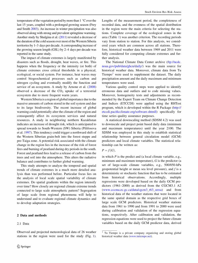
stations in the region were used for the study (Fig. 1).

Lengths of the measurement period, the completeness of

recorded data, and the evenness of the spatial distribution

in the region were the main criteria for selecting the sta-

tions. Complete coverage of the ecological zones in the

area (Table 1) was another criterion. The recording periods

vary from station to station. For this analysis, we consid-

ered years which are common across all stations. There-

fore, historical weather data between 1969 and 2011 were

fully considered for computing climate extremes and fur-

ther analysis.

The National Climate Data Center archive (ftp://ncdc.

noaa.gov/pub/data/ghcn/daily/) was the main source for

historical weather data. Moreover, climate data from Tu

Tiempo1 were used to supplement the dataset. The daily

precipitation amount and the daily maximum and minimum

temperatures were used.

Various quality control steps were applied to identify

erroneous data and outliers and to code missing values.

Moreover, homogeneity tests and adjustments as recom-

mended by the Expert Team on Climate Change Detection

and Indices (ETCCDI) were applied using the RHTest

program, which is developed within the R Package (http://

etccdi.pacificclimate.org/software.shtmll) specifically for

time series quality assurance purposes.

A statistical downscaling method (SDSM 4.2) was used

to downscale and project point based daily data (minimum

and maximum temperatures) until the year 2100. The

SDSM was employed in this study to establish statistical

relationship between general circulation model (GCM)

predictors and local climate variables. The statistical rela-

tionship can be written as:

P ¼ f ðGÞ;

in which P is the predict and (a local climate variable, e.g.,

minimum and maximum temperature), G is the predictor (a

set of large-scale climate variables, e.g., 500/850-hPa

geopotential height or mean sea level pressure), and f is a

deterministic or stochastic function that has to be estimated

from historical observations. Accordingly, multiple

regressions were developed based on the daily GCM pre-

dictors (1961–2000) as derived from the CGCM3.1 A2

(www.cccma.ec.gc.ca/data/cgcm3_t63_sresa) and from

historical data of the weather stations that were located in

the same spatial domain as the respective grid boxes of

large scale GCM predictors. Historical weather stations

data from 1961 to 1990 and from 1991 to 2000 were used

during calibration and validation of the regression equa-

tions, respectively. After calibration and validation, the

regression equations were used to project the future climate

variables based on the daily GCM predictor data, derived

1 Tu Tiempo is a private company organizing and storing global

historical weather data (www.tutiempo.net).

Stoch Environ Res Risk Assess

123

from the CGCM3.1 A2 SRES scenario (www.cccma.ec.gc.

ca/data/cgcm3_t63_sresa).

The A2 SRES emission scenario assumes that regional

heterogeneity, self-reliance of various regions and local

identities are emphasized over the next 100 years and that

economic development is regionally oriented. It is realistic

to consider this emission scenario for a study such as this

present one, focusing on regional and local levels.

2.2 Methods

2.2.1 Climate extreme indices

There are numerous methods and indicators to assess climate

extremes in a changing climate. We refer to the tool developed

by the ETCCDI, which is a joint expert team from CCl2/

CLIVAR3/JCOMM4 (WMO 2009). The tool uses sixteen

temperature-related indices and eleven precipitation-related

indices to extract the occurrence of extreme events in a

meteorological time series. These 27 indices can be calculated

by the RClimDex program, which is developed specifically

for this purpose within the R Package (http://etccdi.pacific

climate.org/list_27_indices.shtml). Ten indices were selected

for this study, taking into account their robustness, their little

correlation with each other, and their potential to exert impact

on ecosystems and human society (Table 2). In addition, the

number of growing degree days (GDDs), which is not inclu-

ded in the standard definitions of indices, was used.

The temperature-based indices are grouped into extreme

value indices, relative indices, and absolute indices (Table 2).

Extreme value indices are indices that utilize extreme values of

the daily maximum and minimum temperatures. Relative

indices are computed based on relative or floating thresholds. In

the calculation of these indices, the 90th (10th) percentile of the

daily maximum (minimum) temperature data of the reference

period are taken as the upper (lower) threshold. Absolute

indices are computed based on original observational data and

fixed thresholds. In the same fashion, the precipitation-based

indices are grouped into relative and absolute indices (Table 2).

All the above 10 indices were computed using observed

and projected climate data of the 26 stations.

2.2.2 Temporal trend

2.2.2.1 Mann–Kendall A non-parametric rank-based

Mann–Kendall (MK) trend test (Mann 1945; Kendall 1975)

was applied to climate extreme indices. It was applied for each

station as well as for the region as a whole after averaging

indices of all stations. The MK test is commonly used for

detecting monotonic increases and decreases in meteorolog-

ical time series (Gemmer et al. 2011; Vincent et al. 2011;

Wang et al. 2012; Yang et al. 2011). In a trend test, the null

hypothesis H0 is that there is no trend in the analyzed time-

series, and hypothesis H1 is that there is a trend in the analyzed

data. The MK test is applied by considering the statistic S as:

S ¼Xn�1

n¼1

Xn

j¼kþ1

sgn Xj � Xk

� �;

where Xj and Xk are the annual values in years j and k,

j [ k, respectively, and

Fig. 1 Map of (a) Russian Federation as a reference to the study area, and (b) weather station distribution in South Western Siberia

2 CCL stands for WMO’s commission for Climatology.3 CLIVAR stands for Climate Varibility and Predicibility.4 JCOMM stands for for WMO-IOC Technical Commission for

Oceanography and Marine Meteorology.

Stoch Environ Res Risk Assess

123

sgn Xj � Xk

� �¼þ1 Xj � Xk

� �[ 0

0 Xj � Xk

� �¼ 0

�1 Xj � Xk

� �\1

������

������:

The MK test has two parameters. One is the significance

level that indicates the test strength and the other one is the

slope magnitude estimate that indicates the direction of the

trend. Under the null hypothesis, xi are independent and

randomly ordered, the statistic S is approximately normally

distributed when n C 8 with zero mean and variance as

Var(S) = n(n - 1)(2n ? 5)/18. The standardized statisti-

cal test (Z) was computed by:

Z ¼

S� 1ffiffiffiffiVp

arðSÞS [ 0

0 S ¼ 0Sþ 1ffiffiffiffiVp

arðSÞS\0

���������

���������

:

At the given significance level a, if |Z| C Z1-a/2, the H0

is rejected, that means the time-series has a trend in the MK

test at significance level a. Furthermore, if Z [ 0, the time-

series has an upward trend, and if Z \ 0, it has a downward

trend.

2.2.3 Spatial gradient

The regional and local spatial gradient of the climate

extreme indices were examined on decadal bases using

multiple linear regressions and a geostatistical function

called semivariogram, respectively. The decades are,

1971–1980, 1981–1990, 1991–2000, 2001–2010,

2011–2020, 2021–2030, 2031–2040, and 2041–2050.

The multiple linear regressions were used to identify the

significant regional spatial gradient of the decadal climate

extreme indices along latitude and longitude. Furthermore,

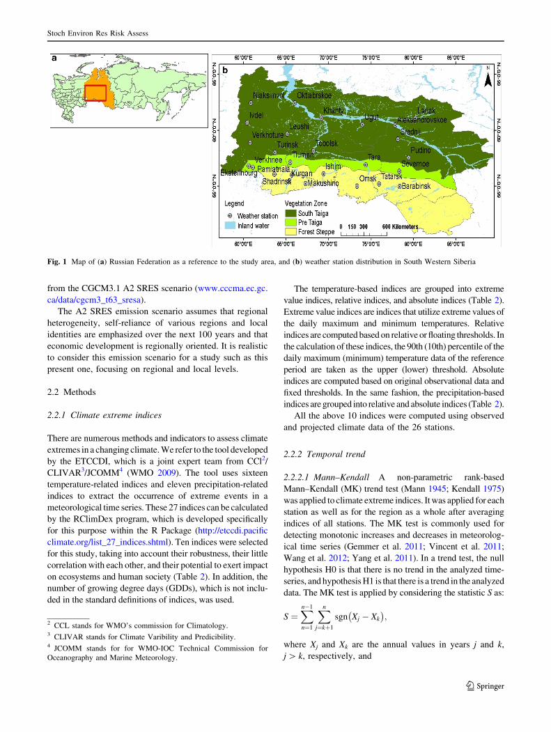
Table 1 Climate characteristics of the weather stations and ecological zones

Numbers Station name Latitude (�) Longitude (�) Altitude (m) Mean annual

precipitation

(mm)

Mean temperature (�C) Vegetation

zonesTmax Tmin

1 Shadrinsk 56.08 63.63 88 455.5 7.8 -1.8 Forest steppe

2 Pamiatnaia 56.02 65.70 66 388.0 7.1 -3.4

3 Ishim 56.10 69.43 81 401.3 6.6 -3.7

4 Kurgan 55.47 65.40 73 385.6 7.7 -2.4

5 Makushino 55.25 67.30 140 362.2 7.1 -2.5

6 Omsk 55.02 73.38 121 411.6 6.9 -2.9

7 Tatarsk 55.20 75.97 110 378.7 7.2 -3.3

8 Barabinsk 55.00 78.37 119 387.7 6.4 -3.7

9 Tiumen 57.15 65.50 79 476.2 7.0 -2.8 Pre-Taiga

10 Ekaterinburg 56.83 60.63 281 517.9 7.4 -1.0

11 Verkhnee 56.70 61.10 286 546.0 6.9 -2.1

12 Tara 56.90 74.39 73 446.3 5.8 -4.4

13 Severnoe 56.35 78.35 124 465.8 5.8 -4.6

14 Niaksimvol 62.43 60.87 51 525.6 3.7 -6.6 South Taiga

15 Oktiabrskoe 62.45 66.05 70 614.1 2.5 -6.0

16 Lariak 61.10 80.25 55 544.8 2.1 -7.1

17 Ivdel 60.68 60.45 93 529.5 5.2 -5.6

18 Khanty 61.07 69.17 46 544.0 3.3 -5.0

19 Ugut 60.50 74.02 47 584.3 2.8 -6.5

20 Aleksandrovskoe 60.43 77.87 47 511.6 3.4 -6.2

21 Leushi 59.67 65.17 70 495.2 5.1 -3.6

22 Verkhoture 58.90 60.79 125 558.6 6.6 -3.7

23 Turinsk 58.04 63.70 103 520.3 6.7 -3.1

24 Tobolsk 58.15 68.25 49 479.3 5.6 -4.0

25 Srednii 59.20 78.20 68 547.7 4.8 -5.1

26 Pudino 57.57 79.43 96 503.1 5.8 -5.6

The station name transliterated after ICAO, passport 2013

Stoch Environ Res Risk Assess

123

the residuals of the fitted regression model were used to

evaluate the local spatial variability by applying a semi-

variogram function. Maps were prepared by interpolating

the multiple linear regression models and kriging of the

residuals through geo-statistical functions. Final maps were

produced by summing the maps that are made from the two

functions.

2.2.3.1 Multiple linear regressions The regional spatial

gradient analysis includes fitting a two-dimensional least

square surface along latitude and longitude as:

Y ¼ bþ a1x1 þ a2x2;

where Y represents the least square value of the particular

climate extreme index and x1 and x2 represent the longitude

and latitude dimensions along which the least square trend

surface is computed. The slopes a1 and a2 indicates the

spatial gradient of the climate indices along longitude and

latitude which are computed in decadal basis. Spatial gra-

dient are obtained for each extreme index on decadal basis

and the statistical significance P of the trends was assessed

by applying the t-statistics in both dimension.

2.2.3.2 Semivariogram The semivariogram is the geo-

statistical key function that is used to characterize the local

spatial variability of climate extremes as based on the

residuals obtained from the multiple linear regression

function. The experimental semivariogram c(h) of the

residue were computed as half the average squared dif-

ference between data pairs belonging to a certain distance

class:

cðhÞ ¼ 1

2NðhÞXNðhÞ

a¼0

Z uað Þ � Z ua þ hð Þ½ �2;

where N(h) is the number of the data pairs, Z(ua) and

Z(ua ? h), available from the n measurements, given

n measurements [Z(ua), a = 1, …, n] from a single

realization.

Sill, partial sill, nugget and range are the semivariogram

parameters, as Fig. 2 presents, that determine the spatial

pattern of the climate extreme index in a given period.

In this study, rang values, which were computed on

decadal basis, were taken as an indicator for the temporal

Table 2 Climate Extreme Indices used in this study

Elements Index Indicators Definitions Units

Temperature

Extreme value indices

TXx Maximum value of

maximum temperature

Maximum value (x) of the daily maximum temperature (TX) in each year �C

TNn Minimum value of

minimum temperature

Minimum value (n) of the daily minimum temperature (TN) in each year �C

Relative indices

TN90p Warm nights Percentage of days when TN [90th %, percentage of time in base period

(1969–2011)

% Days

TX90p Warm days Percentage of days when TX [90th %, percentage of time in base period

(1969–2011)

% Days

Absolute indices

GSL Growing season length Annual (1 Jan–31 Dec) count of days between first and last periods, during which six

consecutive days occurred with daily mean temperature TG [5 �C

Days

GDD Growing degree days Sum of temperature TXþTN2

� �� Tbase within the growing season (Tbase = 5 �C, the

lowest temperature where metabolic processes result in a net substance gain in

above ground biomass)

Degree-

days

Precipitation

Relative indices

R95p Very wet days Annual total precipitation when daily precipitation amount (RR) [95 % percentage

of time in base period (1969–2011)

mm

Absolute indices

Rx5day Max 5-day precipitation

amount

Monthly maximum consecutive 5-day precipitation mm

CDD Consecutive dry days Maximum number of consecutive days with daily precipitation amount (RR)\1 mm Days

R10 Number of heavy

precipitation days

Annual count of days when PRCP [10 mm Days

Stoch Environ Res Risk Assess

123

trend of local based spatial variability of the climate

extreme indices.

2.2.3.3 Mapping The sequential regression kriging

approach was employed to prepare maps by summing the

maps produced by the multiple linear regression equation

and kriging of the residuals, which were analyzed through

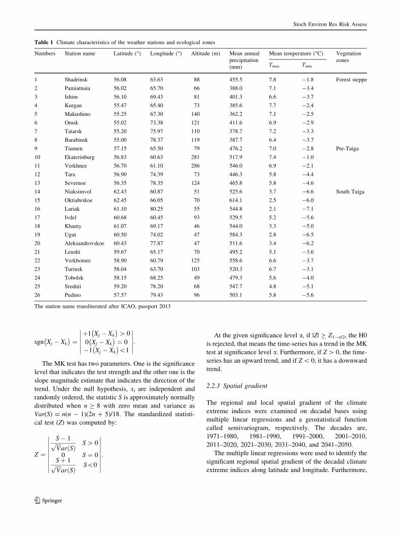
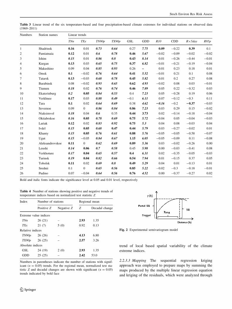
Table 3 Linear trend of the six temperature-based and four precipitation-based climate extremes for individual stations on observed data

(1969–2011)

Numbers Station names Linear trends

TNn TXx TN90p TX90p GSL GDD R10 CDD R95day R95p

1 Shadrinsk 0.16 0.01 0.73 0.64 0.27 7.75 0.09 -0.22 0.39 0.1

2 Pamiatnaia 0.12 0.01 0.6 0.78 0.46 5.67 -0.02 -0.09 -0.02 -0.02

3 Ishim 0.15 0.01 0.86 0.8 0.43 8.14 0.01 -0.26 -0.44 -0.01

4 Kurgan 0.13 0.03 0.65 0.75 0.37 6.82 -0.01 -0.21 -0.19 -0.04

5 Makushino 0.09 0.04 0.85 0.93 0.26 – 0.01 0.23 0.18 0.01

6 Omsk 0.1 -0.02 0.76 0.64 0.41 5.52 -0.01 0.21 0.1 0.08

7 Tatarsk 0.13 -0.03 0.68 0.78 0.45 5.82 0.01 0.2 0.27 0.08

8 Barabinsk 0.08 -0.02 0.93 0.65 0.62 4.93 -0.02 0.08 0.03 -0.01

9 Tiumen 0.18 0.02 0.76 0.74 0.46 7.89 0.05 0.22 -0.32 0.03

10 Ekaterinburg 0.2 0.05 0.84 0.53 0.4 7.23 0.05 -0.28 0.19 0.06

11 Verkhnee 0.17 0.03 0.88 0.49 -0.1 6.11 0.07 -0.12 -0.3 0.11

12 Tara 0.1 0.02 0.64 0.69 0.38 4.62 20.16 -0.2 20.37 -0.03

13 Severnoe 0.09 0 0.86 0.84 0.86 7.23 0.03 0.29 0.15 -0.02

14 Niaksimvol 0.18 0.04 0.6 0.35 0.44 3.73 0.02 -0.14 -0.18 -0.04

15 Oktiabrskoe 0.16 0.05 0.78 0.69 0.75 5.72 -0.04 0.05 -0.04 -0.03

16 Lariak 0.12 0.02 0.83 0.92 0.75 5.3 0.04 0.08 -0.03 0.04

17 Ivdel 0.15 0.05 0.68 0.47 0.44 5.79 0.03 -0.27 -0.02 0.01

18 Khanty 0.15 0.05 0.76 0.61 0.88 5.76 -0.05 -0.05 -0.58 -0.07

19 Ugut 0.15 -0.05 0.84 0.67 1.15 6.05 -0.05 -0.09 0.11 -0.08

20 Aleksandrovskoe 0.11 0 0.62 0.69 0.89 5.36 0.03 -0.02 -0.26 0.00

21 Leushi 0.14 0.06 0.7 0.58 0.45 5.98 0.00 -0.03 -0.41 0.08

22 Verkhoture 0.17 0.04 0.65 0.57 0.4 6.31 0.02 -0.35 -0.05 -0.03

23 Turinsk 0.19 0.04 0.82 0.66 0.54 7.94 0.01 -0.15 0.37 0.05

24 Tobolsk 0.11 0.02 0.69 0.8 0.49 5.29 0.04 0.01 -0.13 0.01

25 Srednii 0.1 0 0.65 0.56 0.85 5.22 -0.02 -0.3 -0.18 -0.01

26 Pudino 0.07 -0.04 0.64 0.56 0.76 4.52 0.00 -0.37 -0.27 0.02

Bold and italic fonts indicate the significance level at 0.05 and 0.01 level, respectively

Table 4 Number of stations showing positive and negative trends of

temperature indices based on normalized test statistic Z

Index Number of stations Regional mean

Positive Z Negative Z Z Decadal change

Extreme value indices

TNn 26 (21) – 2.93 1.35

TXx 21 (7) 5 (0) 0.92 0.13

Relative indices

TN90p 26 (26) – 4.13 6.80

TX90p 26 (25) – 2.57 3.26

Absolute indices

GSL 24 (19) 2 (0) 2.93 1.35

GDD 25 (25) – 2.42 53.0

Numbers in parentheses indicate the number of stations with signif-

icant (a = 0.05) trends. For the regional mean, normalized test sta-

tistic Z and decadal changes are shown with significant (a = 0.05)

trends indicated by bold face

Fig. 2 Experimental semivariogram model

Stoch Environ Res Risk Assess

123

the semivariogram function. The regression kriging equa-

tion can be written as:

z soð Þ ¼ m soð Þ þ e soð Þ;

where z(so) is the final predicted surface, m(so) is the

smoothed surface based on the multiple linear regression

model, and e(so) is the residuals surface interpolated

through simple kriging.

Accordingly, maps of climate extreme indices were pre-

pared for the period (1971–2000) as the reference period, and

for the period (2031–2050) as the future scenario. Further-

more, the change of the spatial trend of the climate extremes

between the two periods was computed in order to identify

areas which will be affected more by climate extremes.

3 Results

The analysis of the temperature- and precipitation-based

climate extreme indices reveal a variety of changes during

the observed (1969–2011) and the projected (2021–2050)

periods.

3.1 Temporal and spatial trends of temperature-based

climate extremes

3.1.1 Extreme value indices

The analysis of the two extreme-value indices, TNn and

TXx, based on the observed data (1969–2011) as shown in

Table 3, exhibits an upward linear trend of 26 stations for

TNn and of 21 stations for TXx. However, only 21 stations

for TNn and 7 stations for TXx are significance at the

a = 0.05 level. Downward trends were observed for TXx

for five stations, however, none of them is significant. The

linear trend of TNn ranges from 0.07 to 0.18 �C year-1.

For TXx, the maximum increase reaches 0.06 �C year-1,

which is quite small as compared to the TNn values.

Regionally computed trends for TNn and TXx show

increases, however, only TNn is significant at the 0.05 level

(Table 4). The regional decadal trend for TNn is 1.35 �C

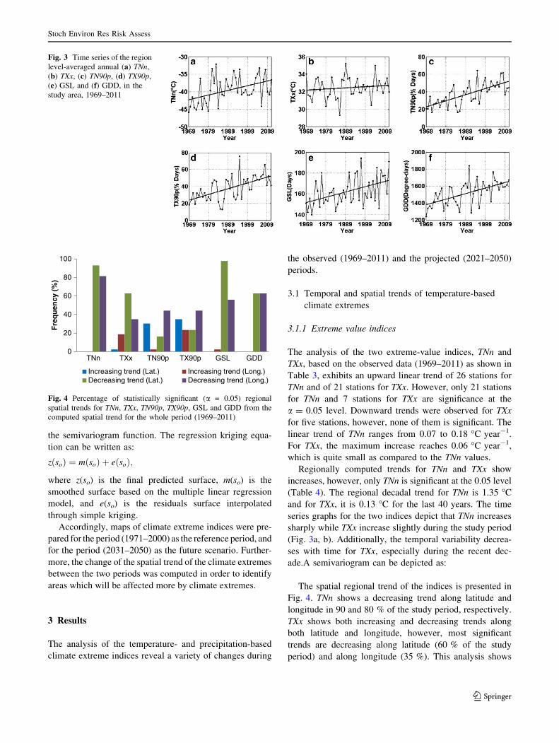
and for TXx, it is 0.13 �C for the last 40 years. The time

series graphs for the two indices depict that TNn increases

sharply while TXx increase slightly during the study period

(Fig. 3a, b). Additionally, the temporal variability decrea-

ses with time for TXx, especially during the recent dec-

ade.A semivariogram can be depicted as:

The spatial regional trend of the indices is presented in

Fig. 4. TNn shows a decreasing trend along latitude and

longitude in 90 and 80 % of the study period, respectively.

TXx shows both increasing and decreasing trends along

both latitude and longitude, however, most significant

trends are decreasing along latitude (60 % of the study

period) and along longitude (35 %). This analysis shows

Fig. 3 Time series of the region

level-averaged annual (a) TNn,

(b) TXx, (c) TN90p, (d) TX90p,

(e) GSL and (f) GDD, in the

study area, 1969–2011

0

20

40

60

80

100

TNn TXx TN90p TX90p GSL GDD

Fre

qu

ency

(%

)

Increasing trend (Lat.) Increasing trend (Long.)Decreasing trend (Lat.) Decreasing trend (Long.)

Fig. 4 Percentage of statistically significant (a = 0.05) regional

spatial trends for TNn, TXx, TN90p, TX90p, GSL and GDD from the

computed spatial trend for the whole period (1969–2011)

Stoch Environ Res Risk Assess

123

that the southern part of the study region is experiencing a

higher increasing rate of these indices than the northern

part.

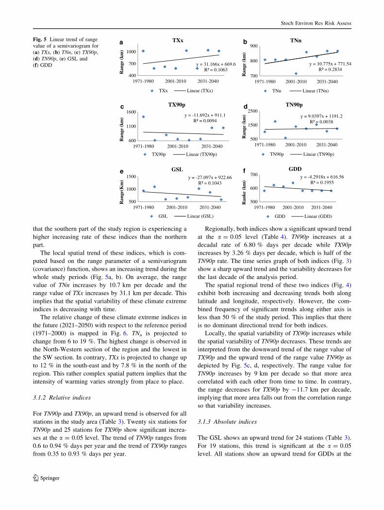
The local spatial trend of these indices, which is com-

puted based on the range parameter of a semivariogram

(covariance) function, shows an increasing trend during the

whole study periods (Fig. 5a, b). On average, the range

value of TNn increases by 10.7 km per decade and the

range value of TXx increases by 31.1 km per decade. This

implies that the spatial variability of these climate extreme

indices is decreasing with time.

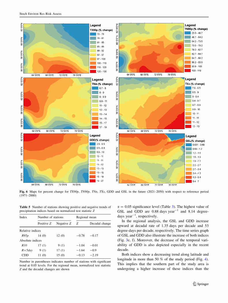
The relative change of these climate extreme indices in

the future (2021–2050) with respect to the reference period

(1971–2000) is mapped in Fig. 6. TNn is projected to

change from 6 to 19 %. The highest change is observed in

the North-Western section of the region and the lowest in

the SW section. In contrary, TXx is projected to change up

to 12 % in the south-east and by 7.8 % in the north of the

region. This rather complex spatial pattern implies that the

intensity of warming varies strongly from place to place.

3.1.2 Relative indices

For TN90p and TX90p, an upward trend is observed for all

stations in the study area (Table 3). Twenty six stations for

TN90p and 25 stations for TX90p show significant increa-

ses at the a = 0.05 level. The trend of TN90p ranges from

0.6 to 0.94 % days per year and the trend of TX90p ranges

from 0.35 to 0.93 % days per year.

Regionally, both indices show a significant upward trend

at the a = 0.05 level (Table 4). TN90p increases at a

decadal rate of 6.80 % days per decade while TX90p

increases by 3.26 % days per decade, which is half of the

TN90p rate. The time series graph of both indices (Fig. 3)

show a sharp upward trend and the variability decreases for

the last decade of the analysis period.

The spatial regional trend of these two indices (Fig. 4)

exhibit both increasing and decreasing trends both along

latitude and longitude, respectively. However, the com-

bined frequency of significant trends along either axis is

less than 50 % of the study period. This implies that there

is no dominant directional trend for both indices.

Locally, the spatial variability of TX90p increases while

the spatial variability of TN90p decreases. These trends are

interpreted from the downward trend of the range value of

TX90p and the upward trend of the range value TN90p as

depicted by Fig. 5c, d, respectively. The range value for

TN90p increases by 9 km per decade so that more area

correlated with each other from time to time. In contrary,

the range decreases for TX90p by -11.7 km per decade,

implying that more area falls out from the correlation range

so that variability increases.

3.1.3 Absolute indices

The GSL shows an upward trend for 24 stations (Table 3).

For 19 stations, this trend is significant at the a = 0.05

level. All stations show an upward trend for GDDs at the

y = 31.166x + 669.6R² = 0.1063

400

700

1000

1971-1980 2001-2010 2031-2040

Ran

ge (k

m)

TXx

TXx Linear (TXx)

a

y = 10.775x + 771.54R² = 0.2834

700

800

900

1971-1980 2001-2010 2031-2040

Ran

ge (k

m)

TNn

TNn Linear (TNn)

b

y = -11.692x + 911.1R² = 0.0094

600

1100

1600

1971-1980 2001-2010 2031-2040

Ran

ge (k

m)

TX90p

TX90p Linear (TX90p)

cy = 9.0397x + 1191.2

R² = 0.0038

500

1500

2500

1971-1980 2001-2010 2031-2040

Ran

ge (k

m)

TN90p

TN90p Linear (TN90p)

d

y = -27.097x + 922.66R² = 0.1043

500

1000

1500

1971-1980 2001-2010 2031-2040

Ran

ge(K

m)

GSL

GSL Linear (GSL)

ey = -4.2918x + 616.56

R² = 0.1955

500

600

700

1971-1980 2001-2010 2031-2040

Ran

ke (

km)

GDD

GDD Linear (GDD)

f

Fig. 5 Linear trend of range

value of a semivariogram for

(a) TXx, (b) TNn, (c) TX90p,

(d) TN90p, (e) GSL and

(f) GDD

Stoch Environ Res Risk Assess

123

a = 0.05 significance level (Table 3). The highest value of

GSL and GDD are 0.88 days year-1 and 8.14 degree-

days year-1, respectively.

In the regional analysis, the GSL and GDD increase

upward at decadal rate of 1.35 days per decade and 53

degree-days per decade, respectively. The time series graph

of GSL and GDD also illustrate the increase of both indices

(Fig. 3e, f). Moreover, the decrease of the temporal vari-

ability of GDD is also depicted especially in the recent

decade.

Both indices show a decreasing trend along latitude and

longitude in more than 50 % of the study period (Fig. 4).

This implies that the southern part of the study area is

undergoing a higher increase of these indices than the

Fig. 6 Maps for percent change for TX90p, TN90p, TNn, TXx, GDD and GSL in the future (2021–2050) with respect to reference period

(1971–2000)

Table 5 Number of stations showing positive and negative trends of

precipitation indices based on normalized test statistic Z

Index Number of stations Regional mean

Positive Z Negative Z Z Decadal change

Relative indices

R95p 14 (0) 12 (0) -0.78 -0.17

Absolute indices

R10 17 (1) 9 (1) -1.04 -0.01

R95day 9 (1) 17 (1) -1.64 -0.9

CDD 11 (0) 15 (0) -0.13 -2.19

Number in parentheses indicates number of stations with significant

trend at 0.05 levels. For the regional mean, normalized test statistic

Z and the decadal changes are shown

Stoch Environ Res Risk Assess

123

northern region. Furthermore, the local spatial variability

of these indices increases with time as it is depicted in

Fig. 5e, f by the downward trend of the respective range

values.

Up to 7 % change for GSL and 27 % change for GDD

are expected in the future period (2021–2050) with respect

to the reference period (1971–2000) in the most northern

part of the region.

3.2 Temporal and spatial trend of precipitation based

climate extremes

Table 5 shows the precipitation indices that are categorized

into a relative precipitation index (R95p) and absolute

precipitation indices (R10, R95day, CDD, SDII). No sig-

nificant trend is observed in any of these indices at the

regional level. However, very few stations show significant

trends for various indices.

3.2.1 Relative indices

Nearly equal numbers of stations show an upward and

downward trend for the R95p index, respectively (Table 3).

Fourteen stations show upward trends and 12 stations show

downward trends. However, none of them are significant at

the a = 0.05 level. The linear trend value ranges from

-0.08 to 0.1 days year-1.

The regional trend of R95p is downward at

-0.17 days year-1. However, the trend is not significant as

well (Table 5).

The time series graph of this index exhibits a slight

downward trend. The very large variability of values,

which is apparent for the time period before the 1990s, is

reduced afterwards (Fig. 7d).

Spatially, there is no dominant direction for the regional

trend of R95p along longitude and latitude. The increasing

and/or decreasing trends of this index in both dimensions

occur during less than 10 % of the study period (Fig. 8).

However, the local variability is reduced as shown by the

increasing trend of the range value of the index (Fig. 9).

This increase amounts to 310 km per decade. In other

words, the numbers of stations that are spatially correlated

are increasing with time.

The 40 years mean spatial pattern of R95p shows that the

highest R95p occurs in a small pocket of land in the south-

eastern part of the study area, and the lowest value occurs

in SW part of the study area (Fig. 10).The middle and

northern part of the region are experiencing moderate

values of the R95p index.

3.2.2 Absolute indices

R10, R95day and CDD are the indices which are catego-

rized as absolute indices. Station-based analysis of these

indices shows that there are upward and downward trends

with only a very few stations showing trends significant at

the a = 0.05 level (Table 3). For the R10 index, 17 stations

show an upward trend and 9 stations show a downward

trend. Only two trends, one of either direction, are signif-

icant at the a = 0.05 level. The highest value reaches to

0.09 days year-1. The regional trend for R10 is downward

but not significant as well. It amounts -0.01 days per

decade. For R95day, the same numbers of stations as in the

case of R10 show trends. However, the trend direction is

opposite. Again, only two stations show significant trends,

one of either direction. The R95day linear trend value

ranges from -0.58 to 0.3 mm year-1 and the regional

trend is -0.9 mm per decade.

Regarding CDD, 11 stations show upward trend and 15

stations show downward trend. None of the trends are

significant for CDD. Its linear trend value ranges from

-0.37 to 0.2 days year-1. No significant trend also

observed for CDD at the regional level (Table 5). Its trend

value amounts -2.19 days per decade. The variability of

R10, R95day, and CDD apparently decrease after the year

2000 (Fig. 7a–c). The regional spatial trend for R10

Fig. 7 Time series of the region level-averaged annual (a) R10,

(b) RX5day, (c) CDD and (d) R95p, in the study area, 1969–2011

0

10

20

30

40

50

60

CDD R10 Rx5day R95p

Fre

qu

ency

(%

)

Increasing trend (Lat.) Increasing trend (Long.)Decreasing trend (Lat.) Decreasing trend (Long.)

Fig. 8 Percentage of statistically significant (a = 0.05) regional

spatial trend for CDD, R10, R95day and R95p from the computed

spatial trend for the whole period (1969–2011)

Stoch Environ Res Risk Assess

123

exhibits an increasing trend along latitude in nearly 50 %

of the analysis period, and a decreasing trend along lon-

gitude during 30 % of the analysis period (Fig. 8). For

CDD, the decreasing trend along latitude is relatively

dominant and amounts nearly 30 % of the study period.

The R10 and CDD indices exhibit an increase of range

value with a linear trend of 251 and 271 km per decade,

respectively (Fig. 9a, b).This implies that more stations are

becoming correlated to each other over time. For R95day,

the range value rather decreases at a linear rate of

y = 271.55x + 704.41R² = 0.8797

800

1300

1800

1971-1980 1981-1990 1991-2000 2001-2010

Ran

ge(k

m)

CDD

CDD Linear (CDD)

a

y = -122.59x + 1184R² = 0.3643

400

900

1400

1971-1980 1981-1990 1991-2000 2001-2010

Ran

ge (k

m)

RX5day

RX5day Linear (RX5day)

b

y = 151.49x + 538.98R² = 0.6154

400

900

1400

1971-1980 1981-1990 1991-2000 2001-2010

Ran

ge (k

m)

R10

R10 Linear (R10)

c

y = 310.98x + 149.54R² = 0.7466

0

1000

2000

1971-1980 1981-1990 1991-2000 2001-2010

Ran

ge (k

m)

R95p

R95p Linear (R95p)

d

Fig. 9 Linear trend of range

value of a semivariogram for

(a) CDD, (b) R95day, (c) R10

and (d) R95p

Fig. 10 Mean spatial pattern of R95p, R95day, R10 and CDD in the past (1969–2011)

Stoch Environ Res Risk Assess

123

-122 km per decade. In other words, local variability

increases with time for this index.

For the mean spatial pattern for R10, the highest value

13.2 days year-1 occurs in the North-Western part and it

decreases to the south-east to the value of 5.5 days year-1

(Fig. 10). The R95day follow a similar pattern except very

few pocket areas experiencing higher values. The highest

value in the east part of the study area reaches to

67.5 mm year-1. In contrary, the highest CDD values are

found in the southern part of the study area. However, small

pockets of land in the south also experience a lower CDD

value. The Highest CDD value reaches to 58.8 days year-1

and the lowest reaches to 29.4 days year-1.

4 Discussion and conclusion

The analysis of various climate extreme indices based on

the observed and projected climate data have evidenced

significant upward trends for most of temperature-based

indices while the precipitation-based climate extremes

indices showed no significant trend at all. This mirrors

studies at the global level that also found that precipitation-

based extremes are less significant than those based on

temperatures (Alexander et al. 2006).

The regional time series graphs of the climate extreme

indices reveal that the variability is decreasing through

time for most indices, especially during the last decades or

after 2000. This decrease in temporal variability of the

climate indices is also reflected by the decrease of the

spatial variability through time for most indices, as indi-

cated by the increasing trend of the range value of the

semivariogram function computed for individual climate

extreme indices. This decrease of variability implies that a

larger area is becoming similar, meaning that the study area

becoming more homogenous. This tendency may indicate

that the large-scale atmospheric patterns are becoming

more dominant as compared to the local factors which are

responsible for variations of the climate extremes at local

level. An earlier study for the area showed that the large

scale atmospheric pattern, Arctic Oscillation, explains

53 % of temperature variation in Western Siberia (Frey and

Smith 2003).

The regional spatial pattern of the climate extreme

analysis shows that the temperature-based climate

extremes, TNn, TXx, GSL and GDD, decrease while the

precipitation-based climate extremes, R10 and R95day,

increase along latitude and longitude for more than half of

the analysis period. Relatively, the southern part of the

region becomes drier and warmer and the northern part

becomes wetter and less warmer compared to the south.

The higher value and frequency of the CDD index confirms

that the southern region experiences more drought events

as well. Hence, it is apparent that the southern part of the

study area, which is classified as forest steppe, is influenced

more by environmental stress than areas in the north, the

pre-Taiga and south Taiga. This tendency indicates the

potential effect of climate change to foster a northward

shift of the West-Siberian grain belt into the forest steppe

and pre-Taiga zone in addition to the landuse/cover change

that is the main driver in the area. This reasoning is further

confirmed by the larger change of the projected bio-climate

indicators, length of the growing season (GSL) and GDDs,

in the north.

In relation to the climate extremes, some finger prints of

extreme events have been observed in the region during

recent decades. For instance, the fire risk intensity

increased in the study region during the last decade

(Balzter et al. 2010; Stocks et al. 1998). Forest fires lead to

the release of enormous amounts of stored carbon into the

atmosphere. Besides the forests, peatlands are also affected

by fire causing significant losses of carbon (Houghton

2003; Wirth et al. 2002; Schulze and Freibauer 2005).

Moreover, indications of agricultural drought in the

southern steppe part of the study region were reported by

researchers working in the area. In response, field experi-

mentation of drought-resistant varieties (e.g., wheat) has

been initiated during the last few years.

All in all, this study presents the temporal and spatial

pattern of climate extremes. The changes in intensity and

frequency of climate extremes are becoming the main

threat for the region. Various ecosystems in the area are

negatively affected.

The statistical approach which is used in this study opens

the possibility to analyze the spatio-temporal dynamics of

climate extremes at local and regional scales and in long-

term data sets combining past and projected future time

periods. As a result, specific and rather precise recommen-

dations can be developed for agriculture, forest management,

and protection of nature and biodiversity, which can be used

to develop climate change adaptation strategies.

Acknowledgments This work was conducted as part of Project

SASCHA (‘Sustainable land management and adaptation strategies to

climate change for the Western Siberian corn-belt’). We are grateful

for funding by the German Government, Federal Ministry of Edu-

cation and Research within their Sustainable Land Management

funding framework (funding reference 01LL0906D). Degefie T. De-

gefie received additional funding by the German Academic Exchange

Service (DAAD). We thank the two anonymous reviewers for very

helpful comments on an earlier version of the manuscript.

References

Alexander LV, Zhang X, Peterson TC, Caesar J, Gleason B, Tank

MGK, Haylock M, Collins D, Trewin B, Rahimzadeh F,

Tagipour A, Rupa Kumar K, Revadekar J, Griffiths G, Vincent

Stoch Environ Res Risk Assess

123

L, Stephenson DB, Burn J, Aguilar E, Brunet M, Taylor M, New

M, Zhai P, Rusticucci M, Vazquez-Aguirre JL (2006) Global

observed changes in daily climate extremes of temperature and

precipitation. J Geophys Res 111:D05109. doi:10.1029/

2005JD006290

Arnone JA, Verburg PSJ, Johnson DW, Larsen JD, Jasoni RL,

Lucchesi AJ, Batts CM, von Nagy C, Coulombe WG, Schorran

DE, Buck PE, Braswell BH, Coleman JS, Sherry RA, Wallace

LL, Luo Y, Schimel DS (2008) Prolonged suppression of

ecosystem carbon dioxide uptake after an anomalously warm

year. Nature 455(7211):383–386

Balzter H et al (2010) Environmental change in Siberia: earth

observation, field studies and modeling. In: Balzter H (ed)

Advances in global change research, vol 40. Springer, Dordrecht.

doi:10.1007/978-90-481-8641-9_2

Frey KE, Smith LC (2003) Recent temperature and precipitation

increases in West Siberia and their association with the Arctic

Oscillation. Polar Res 22:287–300

Gemmer M, Fischer T, Jiang T (2011) Trends in precipitation

extremes in the Zhujiang River Basin, South China. J Clim

24:750–761

Houghton RA (2003) Revised estimates of the annual net flux of

carbon to the atmosphere from changes in land use and land

management 1850–2000. Tellus B 55:378–390

IPCC (2007a) In: Parry ML, Canziani OF, Palutikof JP, van der

Linden PJ, Hanson CE (eds) Climate change 2007: impacts,

adaptation and vulnerability. Contribution of Working Group II

to the Fourth Assessment Report of the Intergovernmental Panel

on Climate Change. Cambridge University Press, Cambridge

IPCC (2007b) Summary for policymakers. In: Solomon S, Qin D,

Manning M, Chen Z, Marquis M, Averyt KB, Tignor M, Miller

HL (eds) Climate change 2007: the physical science basis.

Contribution of Working Group I to the Fourth Assessment

Report of the Intergovernmental Panel on Climate Change.

Cambridge University Press, Cambridge

IPCC (2012) In: Field CB, Barros V, Stocker TF, Qin D, Dokken DJ,

Ebi KL, Mastrandrea MD, Mach KJ, Plattner G-K, Allen SK,

Tignor M, Midgley PM (eds) Managing the risks of extreme

events and disasters to advance climate change adaptation.

A Special Report of Working Groups I and II of the

Intergovernmental Panel on Climate Change. Cambridge Uni-

versity Press, Cambridge

Kendall MG (1975) Rank correlation methods. Griffin, London

Kharin V, Zwiers FW, Zhang X, Hegerl GC (2007) Changes in

temperature and precipitation extremes in the IPCC ensemble of

global coupled model simulations. J Clim 20(8):1419–1444

Mann HB (1945) Nonparametric tests against trend. Econometrica

13:245–259

Pilifosova O, Eserkepova I, Dolgih S (1997) Regional climate change

scenarios under global warming in Kazakhstan. Clim Change

36:23–40

Schulze ED, Freibauer A (2005) Environmental science—carbon

unlocked from soils. Nature 437:205–206

Shulgina TM, Genina EYu, Gordov EP (2011) Dynamics of climatic

characteristics influencing vegetation in Siberia. Environ Res

Lett 6:045210

Stocks BJ, Fosberg MA, Lynham TJ, Mearns L, Wotton BM, Yang Q,

J-Z Jin, Lawrence K, Hartlet GR, Mason JA, McKenney DW

(1998) Climate change and forest fire potential in Russian and

Canadian boreal rorests. Climatic Change 38:1-1

Vincent LA et al (2011) Observed trends in indices of daily and

extreme temperature and precipitation for the countries of the

western Indian Ocean, 1961–2008. J Geophys Res 116:D10108.

doi:10.1029/2010JD015303

Wang W, Shao Q, Yang T, Peng S, Yu Z, Taylor J, Xing W, Zhao C,

Sun F (2012) Changes in daily temperature and precipitation

extremes in the Yellow River Basin, China. Stoch Environ Res

Risk Assess Springer. doi:10.1007/s00477-012-0615-8

Wirth C, Czimczik CI, Schulze ED (2002) Beyond annual budgets:

carbon flux at different temporal scales in fire-prone Siberian

Scots pine forests. Tellus B 54:611–630

WMO (2009) In: Klein Tank AMG, Zwiers FW, Zhang X, Royal

Netherlands Meteorological Institute (eds) Guidelines on Ana-

lysis of extremes in a changing climate in support of informed

decisions for adaptation. Environment Canada

Yang T, Wang X, Zhao C, Chen X, Yu Z, Shao Q, Xu C-Y, Xia J,

Wang W (2011) Changes of climate extremes in a typical arid

zone: observations and multimodel ensemble projections. J Geo-

phys Res 116:D19106. doi:10.1029/2010JD015192

Stoch Environ Res Risk Assess

123