CLIMATE CHANGE MONITORING REPORT 2004

September 2005

JAPAN METEOROLOGICAL AGENCY

Preface

There has been a serious concern of the global society on the climate adversely affected by human activities such as massive consumption of fossil fuels as a result of fast-growing population and industrial development. Particularly, possible climate change including global warming attracts increasing attention of the people and is considered as a critical issue for humankind to be addressed with extreme urgency.

The Intergovernmental Panel on Climate Change (IPCC), which was established

by the United Nations in 1988, has published three Assessment Reports in order to deliver most reliable scientific reviews on climate change, compiling all of updated information and knowledge. The third Report issued in 2001 indicated and projected continual increase in the global average temperature along with increase in greenhouse gas concentrations in the atmosphere. It also suggested a strong possibility of higher frequency of extreme weathers such as torrential rain and severe drought. Under these circumstances, Japan as well as many countries is urged to take immediate actions to fulfill its commitment to reduce greenhouse gas emissions specified in the Kyoto Protocol which came into force in February 2005.

The Japan Meteorological Agency (JMA), in close cooperation with national and

international authorities concerned including the World Meteorological Organization (WMO), is concentrating its efforts in observation and monitoring of climate change as well as elucidating its mechanism. “Climate Monitoring Report” is a yearly outcome of these activities of JMA, which has been providing up-to-date information on climatic conditions around the globe on an annual basis since 1996.

The present issue “Climate Monitoring Report 2004” indicates the continued rise

in the concentration of carbon dioxide and the growing trend in annual-mean temperatures around the globe, while highlighting the second highest record of the annual-mean temperature over Japan in 2004 for the past 100 years and the fourth highest of the global average for the past 120 years. The Report also discusses key factors of the frequent occurrence of unusual weather events in Japan such as frequent occurrence of torrential rains and many landings of typhoons during the summer through autumn in 2004.

It is my hope that readers of the Report will find in it a wealth of information and

knowledge to lead to a better appreciation of climate and to protection as well as preservation of our earth environment.

Finally, I deeply appreciate the individual members of the Advisory Group of the Council

for Climatic Issues under the chairmanship of Prof. K. Hanawa for the pertinent comments and outstanding guidances to us through compiling and editing the Report.

(Koichi Nagasaka) Director-General

Japan Meteorological Agency

Contents 1. Global climate change 1 1.1 Global climate 1 1.2 Surface temperature and precipitation 5 1.3 El Niño / La Niña 9 1.4 Global sea surface temperatures 13 1.5 Sea ice in the Arctic and Antarctic areas 13 2. Climate change in Japan 15 2.1 Climate of Japan 15 2.2 Major meteorological disasters 20 2.3 Surface temperature and precipitation 23 2.4 Tropical storms 24 2.5 Sea surface temperatures in the western North Pacific 26 2.6 Sea ice in the Sea of Okhotsk 27 2.7 Sea level trend around Japan 28 3. Monitoring of greenhouse gases and ozone depleting substances 32 3.1 Greenhouse gases and ozone depleting substances in the atmosphere 32 3.2 Oceanic carbon dioxide 43 3.3 Aerosols 45 4. Monitoring of the ozone layer and ultraviolet B (UV-B) radiation 50 4.1 Observational results of the ozone layer 50 4.2 Solar UV radiation 53 References 56 Map1 Geographical subdivision of Japan 58 Map2 Distribution of surface meteorological observation stations in Japan 59

1

1. Global climate change

Climate changes on different time scales of weeks, seasons, years, decades and even longer periods, with complicated interactions among the atmosphere, the oceans, the cryosphere, the surface lithosphere, and the biosphere, which comprise a climate system. It is also affected by natural and anthropogenic perturbations to the composition of the atmosphere, such as volcanic eruptions and emissions of greenhouse gases associated with human activities.

To monitor the climate change, the Japan Meteorological Agency (JMA) conducts various observations including surface, upper air and oceanographic observations. JMA also collects observational data from all over the world and analyzes them. For example, extreme weather events are operationally monitored with surface meteorological data received from about 1,200 stations in the world through the Global Telecommunication System (GTS) coordinated by the World Meteorological Organization (WMO).

JMA also monitors oceanographic conditions, including ENSO events, which have impacts on the global climate, by collecting oceanographic observations from research vessels, commercial ships, buoys and satellites. 1.1 Global climate 1.1.1 Major climate anomalies

Annual mean temperature anomalies normalized by the standard deviation and annual total precipitation ratios in 2004 are shown in Figure 1.1 and Figure 1.2, respectively. The climatological normals for temperature and precipitation are calculated from the statistics of 1971-2000. The annual mean temperatures were higher than normal in most of the world. The annual total precipitations were above normal in eastern and central Canada, northwestern Australia, from southern USA to northern Mexico and from central Asia to western Russia, while they were below normal in central and eastern Australia, from western India to Pakistan and from western Canada to eastern Alaska.

Global climatic highlights in 2004 are summarized in Figure 1.3. It indicates the areas where warm/cold or wet/dry conditions continued for more than three months. Warm conditions continued in East Asia and Micronesia for most of the year, and in the western coast of North America from spring to autumn. Persistent wet conditions often appeared in southern Canada. On the other hand, persistent dry conditions often appeared in western North America and Australia.

2

Very Warm 　□ Warm　　 　○Normal(+)

Very Cold ■ Cold　　　 　●Normal(-)

Very Warm 　□ Warm　　 　○Normal(+)

Very Cold ■ Cold　　　 　●Normal(-)

Figure 1.1 Annual mean temperature in 2004.

Categories are defined by annual mean of normalized monthly temperature anomaly against normal (1971-2000 average).

● Wet　 ● Normal(+)

○ Dry　 ○ Normal(-)

● Wet　 ● Normal(+)

○ Dry　 ○ Normal(-)

Figure 1.2 Annual total precipitation in 2004

Categories are defined by annual precipitation ratio to normal (1971-2000 average).

3

H:Jan.-Apr.

H:Jan.-Mar.

H:Jan.-Mar.

H:Jan.-Apr./ H:Jul.-Oct.

NO DATA

H:Jan.-Nov.

H:Jan.-Apr.

C:May-Jul.

H:Jan.-Mar.

H:Jan.-Mar./ Oct.-Dec.

C:Jun.-Aug.

H:Jan.-Apr.

H:Jan.-Dec.

H:Jan.-Mar.

H:Jan.-Mar.

C:Jan.-Mar.

H:Jan.-Apr.

C:Feb.-Apr.

C:May-Jul.

C:May-Jul.

H:Mar.-Jun.

H:Mar.-MayH:Mar.-Sep.

H:Feb.-Jul.

H:Mar.-MayH:Mar.-Nov.

H:Jan.-.May

H:Apr.-Jun.

H:Feb.-Ma y H:Feb.-Nov.

H:Jul.-Nov.

C:Jul.-Nov.

H:Jul.-Dec.

H:Jun.-Nov.

H:Jul.-Oct.

H:Sep.-Dec.

H:Sep.-Nov.

H:Sep.-Nov.H:Mar.-Nov.

H:Mar.-Oct.

H:Mar.-Dec.

H:Jun.-Dec.

H:Aug.-Dec.

H:Oct.-Dec.

H:Oct.-Dec.

H:Oct.-Dec.H:Mar.-Jun. H:Mar.-May

H:Jan.-Apr.

H:Jan.-Mar.

H:Jan.-Mar.

H:Jan.-Apr./ H:Jul.-Oct.

NO DATA

H:Jan.-Nov.

H:Jan.-Apr.

C:May-Jul.

H:Jan.-Mar.

H:Jan.-Mar./ Oct.-Dec.

C:Jun.-Aug.

H:Jan.-Apr.

H:Jan.-Dec.

H:Jan.-Mar.

H:Jan.-Mar.

C:Jan.-Mar.

H:Jan.-Apr.

C:Feb.-Apr.

C:May-Jul.

C:May-Jul.

H:Mar.-Jun.

H:Mar.-MayH:Mar.-Sep.

H:Feb.-Jul.

H:Mar.-MayH:Mar.-Nov.

H:Jan.-.May

H:Apr.-Jun.

H:Feb.-Ma y H:Feb.-Nov.

H:Jul.-Nov.

C:Jul.-Nov.

H:Jul.-Dec.

H:Jun.-Nov.

H:Jul.-Oct.

H:Sep.-Dec.

H:Sep.-Nov.

H:Sep.-Nov.H:Mar.-Nov.

H:Mar.-Oct.

H:Mar.-Dec.

H:Jun.-Dec.

H:Aug.-Dec.

H:Oct.-Dec.

H:Oct.-Dec.

H:Oct.-Dec.H:Mar.-Jun. H:Mar.-May

W:Jan.-Mar.

NO DATA

D:Jan.-Mar.

W:Jan.-Mar.

W:Jan.-Mar.

D:Mar.-Jul.

D:Mar.-Jul.

D:Mar.-May D:Jan.-Mar.

D:May-Jul.

D:Jan.-Mar.

D:Jul.-Sep.

W:Sep.-Nov.

W:Jan.-Mar.

D:Feb.-Apr.

W:Mar.-May

W:Mar.-May

W:Jul.-Sep.

W:Sep.-Nov.

D:Oct.-Dec.

W:Oct.-Dec.

D:Oct.-Dec.

W:Oct.-Dec.

D:May-Sep.

W:Jan.-Mar.

NO DATA

D:Jan.-Mar.

W:Jan.-Mar.

W:Jan.-Mar.

D:Mar.-Jul.

D:Mar.-Jul.

D:Mar.-May D:Jan.-Mar.

D:May-Jul.

D:Jan.-Mar.

D:Jul.-Sep.

W:Sep.-Nov.

W:Jan.-Mar.

D:Feb.-Apr.

W:Mar.-May

W:Mar.-May

W:Jul.-Sep.

W:Sep.-Nov.

D:Oct.-Dec.

W:Oct.-Dec.

D:Oct.-Dec.

W:Oct.-Dec.

D:May-Sep.

Figure 1.3 Significant climate anomalies in the world in 2004

Top : major areas where temperature in warm/cold-category continued for three months or more. Solid red lines with "H" mean "warm" (high temperature), while dashed blue lines with "L" mean "cold" (low temperature).

Bottom : major areas where precipitation in wet/dry-category continued for three months or more. Solid green lines with "W" mean "wet" (heavy precipitation), while dashed orange lines with "D" mean "dry" (light precipitation).

4

Fores t fire Jun.-Sep.

Drought Jun.-Jul.

DroughtJun.-Jul.

Heavy rain,TyphoonJun.-Oct.

　　　 Storm　　　　Oct.(west), Nov.(East)

Cold waveJun.-Jul.

Heavy rain MayHurricane Aug.-Sep.

Cyclone, Heavy rainApr.-Oct.

Heat wave,Fores t fireJun.-Jul.

CycloneMar.

Cold waveJan.(East), Feb.(South)

DroughtSep.-Nov.

Cold waveDec.-Jan.

Heavy rain, Heavy snow

Dec.HurricaneAug.-Sep.

Typhoon Ma y-Jul.,Nov.-Dec.

Heavy rainMar.-Apr.

Heavy rainApr.-Ma y

Thunder s torm , Tornado May

Heavy rain,Typhoon Jun.-Nov.

Heavy rainDec.

Fores t fireOct.

Cold wave, StormJan.-Feb.

Heavy rainJan.-Feb.

Fores t fire Jun.-Sep.

Drought Jun.-Jul.

DroughtJun.-Jul.

Heavy rain,TyphoonJun.-Oct.

　　　 Storm　　　　Oct.(west), Nov.(East)

Cold waveJun.-Jul.

Heavy rain MayHurricane Aug.-Sep.

Cyclone, Heavy rainApr.-Oct.

Heat wave,Fores t fireJun.-Jul.

CycloneMar.

Cold waveJan.(East), Feb.(South)

DroughtSep.-Nov.

Cold waveDec.-Jan.

Heavy rain, Heavy snow

Dec.HurricaneAug.-Sep.

Typhoon Ma y-Jul.,Nov.-Dec.

Heavy rainMar.-Apr.

Heavy rainApr.-Ma y

Thunder s torm , Tornado May

Heavy rain,Typhoon Jun.-Nov.

Heavy rainDec.

Fores t fireOct.

Cold wave, StormJan.-Feb.

Heavy rainJan.-Feb.

Figure 1.4 Climate-related disasters in 2004 1.1.2 Regional anomalies and events

Figure 1.4 shows major climate-related disasters in 2004. Descriptions about disasters in the following paragraphs are based on press articles. Extremely high/low temperature and heavy/light precipitation are defined as the values which are observed once in 30 years or more. Regional climate anomalies and events are as follows. (1) East Asia and Siberia The annual mean temperatures were higher than normal except for part of Siberia. Unusually high temperatures were observed from East Asia to Central Asia. The annual precipitaions were above normal in northern China and from western China to central Asia. It was reported that damages were caused by heavy rain and typhoons in Japan, China and the Korean Peninsula from June to October. In particular, in eastern China, more than 400 fatalities and missing persons were reported. On the other hand, it was reported that devastating droughts continued in southern China for the first time in 54 years and caused shortages of drinking water and damages to crops from September to November. (2) Southern Asia The annual mean temperatures were higher than normal except for part of Thailand. The annual precipitaions were above normal in eastern India, while they were below normal from western India to Pakistan. It was reported that in northern India and Bangladesh, more than 600 fatalities were caused by cold waves accompanied with thick mists from the end of December 2003 to the beginning of January 2004. It was reported that, during rainy season, at least 2000 fatalities and massive damages to agricultural fields were caused by heavy rain in India, Bangladesh and Nepal from June to October. On the other hand, from May to July and from the end of November to the beginning of December, it was reported that several typhoons and a tropical depression landfalled on the Philippines, which resulted in more than 1,500 fatalities. (3) Europe The annual mean temperatures were higher than normal in most of Europe. Unusually high temperatures were observed in northwestern Europe.

5

The annual precipitaions were above normal in northeastern Europe and western Russia. Warm and dry conditions brought by strong subtropical high continued from June to July in southern Europe. During the period, it was reported that 11 and 33 fatalities were caused by heat waves in Spain and southeastern Europe, respectively. It was also reported that many wildfires destroyed 1,450 km2 of forests in Spain and Portugal. (4) Africa and the Middle East The annual mean temperatures were higher than normal in most of the areas where the observation data were reported. Unusually high temperatures were observed in western Africa, around Egypt and from South Africa to Madagascar. The annual precipitaions were above normal in western Africa and northern Turkey, while they were below normal in western and southern Saudi Arabia. More than 280 fatalities were caused by the cyclone “Gafilo” were reported in Madagascar in the first half of March. On the other hand, extensive droughts were reported in Ethiopia and southern Africa. (5) North America The annual mean temperatures were higher than normal in western North America, while they were below normal in northern North America. The annual precipitaions were above normal in eastern and central Canada, western Alaska and from southern USA to northern Mexico, while they were below normal from western Canada to eastern Alaska where dry conditions were likely to continue from May to September. In Alaska, the worst wildfires in its histories were reported. On the other hand, it was reported that some hurricanes affected from southeastern USA to Caribbean Islands from August to September. Especially, it was reported that hurricane “Jeanne” resulted in more than 3,000 fatalities in Haiti. In Haiti, more than 1,000 fatalities caused by heavy rain were also reported in the end of May. (6) South America The annual mean temperatures were higher than normal in most of the areas where the observation data were reported. Unusually high temperatures were observed in southern Argentina. The annual precipitations were above normal in Venezuela, northeastern Brazil and southern South America. In Brazil, it was reported that floods and landslides resulted in more than 160 fatalities from December to February. (7) Oceania The annual mean temperatures were higher than normal except for Australia and New Zealand. The annual precipitations were above normal in northern Australia, while they were below normal in central and eastern Australia where dry conditions has continued for a few years. 1.2 Surface temperature and precipitation

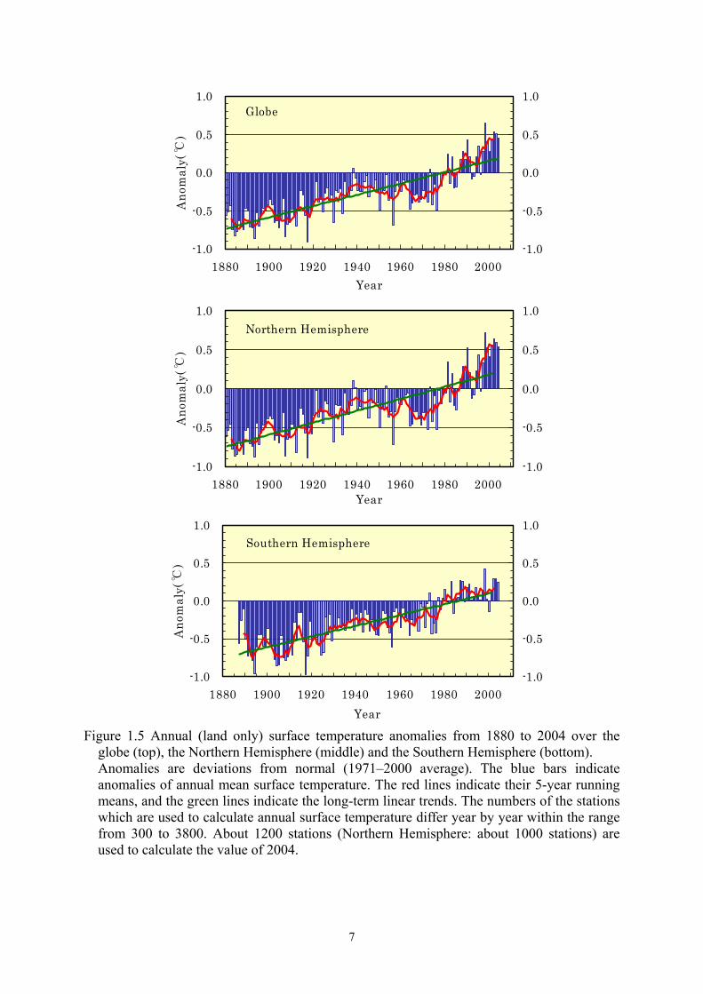
The global mean surface temperature in 2004 was +0.45°C above normal (1971–2000

average), and was the forth highest after 1998, 2002, 2003 in the last 125 years. Trends in global (land area only) surface temperature and precipitation are studied from

global observational records since 1880. The annual mean surface temperature has varied in different time scales from a few years to several decades. In a longer time scale, the global mean temperature has been rising at a rate of about 0.7°C per 100 years (Figure 1.5). In

6

particular, the temperature in the Northern Hemisphere has considerably increased. The global temperature rise of such long-term is likely to have been due to human activities, particularly the emission of greenhouse gases.

The global annual precipitation ratio in 2004 to normal (1971–2000 average) was 102%. The precipitation also has variations of different time scales (Figure 1.6). There has been

small positive trend in the Southern Hemisphere, but in the Northern Hemisphere no remarkable trend can be seen.

7

Globe

-1.0

-0.5

0.0

0.5

1.0

1880 1900 1920 1940 1960 1980 2000Year

Ano

mal

y(℃

)

-1.0

-0.5

0.0

0.5

1.0

Northern Hemisphere

-1.0

-0.5

0.0

0.5

1.0

1880 1900 1920 1940 1960 1980 2000Year

Ano

mal

y(℃

)

-1.0

-0.5

0.0

0.5

1.0

Southern Hemisphere

-1.0

-0.5

0.0

0.5

1.0

1880 1900 1920 1940 1960 1980 2000Year

Ano

mal

y(℃

)

-1.0

-0.5

0.0

0.5

1.0

Figure 1.5 Annual (land only) surface temperature anomalies from 1880 to 2004 over the

globe (top), the Northern Hemisphere (middle) and the Southern Hemisphere (bottom). Anomalies are deviations from normal (1971–2000 average). The blue bars indicate anomalies of annual mean surface temperature. The red lines indicate their 5-year running means, and the green lines indicate the long-term linear trends. The numbers of the stations which are used to calculate annual surface temperature differ year by year within the range from 300 to 3800. About 1200 stations (Northern Hemisphere: about 1000 stations) are used to calculate the value of 2004.

8

Globe

80

90

100

110

120

1880 1900 1920 1940 1960 1980 2000Year

Rat

io(%

)

80

90

100

110

120

Northern Hemisphere

80

90

100

110

120

1880 1900 1920 1940 1960 1980 2000Year

Rat

io(%

)

80

90

100

110

120

Southern Hemisphere

80

90

100

110

120

1880 1900 1920 1940 1960 1980 2000Year

Rat

io(%

)

80

90

100

110

120

Figure 1.6 Annual (land only) precipitation ratios from 1880 to 2004 over the globe (top), the

Northern Hemisphere (middle) and the Southern Hemisphere (bottom). The blue lines indicate annual precipitation ratios to normal (1971–2000 average). The red lines indicate their 5-year running means. The numbers of the stations which are used to calculate annual surface temperature differ year by year within the range from 300 to 3800. About 1200 stations (Northern Hemisphere: about 1000 stations) are used to calculate the value of 2004.

9

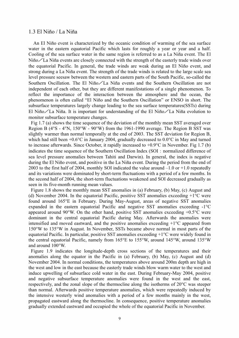
1.3 El Niño / La Niña An El Niño event is characterized by the oceanic condition of warming of the sea surface

water in the eastern equatorial Pacific which lasts for roughly a year or year and a half. Cooling of the sea surface water in the same region is referred to as a La Niña event. The El Niño／La Niña events are closely connected with the strength of the easterly trade winds over the equatorial Pacific. In general, the trade winds are weak during an El Niño event, and strong during a La Niña event. The strength of the trade winds is related to the large scale sea level pressure seesaw between the western and eastern parts of the South Pacific, so-called the Southern Oscillation. The El Niño／La Niña events and the Southern Oscillation are not independent of each other, but they are different manifestations of a single phenomenon. To reflect the importance of the interaction between the atmosphere and the ocean, the phenomenon is often called “El Niño and the Southern Oscillation” or ENSO in short. The subsurface temperatures largely change leading to the sea surface temperatures(SSTs) during El Niño／La Niña. It is important for understanding of the El Niño／La Niña evolution to monitor subsurface temperature changes. Fig 1.7 (a) shows the time sequence of the deviation of the monthly mean SST averaged over Region B (4°S - 4°N, 150°W - 90°W) from the 1961-1990 average. The Region B SST was slightly warmer than normal temporally at the end of 2003. The SST deviation for Region B, which had still been +0.6°C in January 2004, gradually decreased to 0.0°C in May and turned to increase afterwards. Since October, it rapidly increased to +0.9°C in November. Fig 1.7 (b) indicates the time sequence of the Southern Oscillation Index (SOI：normalized difference of sea level pressure anomalies between Tahiti and Darwin). In general, the index is negative during the El Niño event, and positive in the La Niña event. During the period from the end of 2003 to the first half of 2004, monthly SOI indicated the value around –1.0 or +1.0 repeatedly and its variations were dominated by short-term fluctuations with a period of a few months. In the second half of 2004, the short-term fluctuations weakened and SOI decreased gradually as seen in its five-month running mean values. Figure 1.8 shows the monthly mean SST anomalies in (a) February, (b) May, (c) August and (d) November 2004. In the equatorial Pacific, positive SST anomalies exceeding +1°C were found around 165°E in February. During May-August, areas of negative SST anomalies expanded in the eastern equatorial Pacific and negative SST anomalies exceeding -1°C appeared around 90°W. On the other hand, positive SST anomalies exceeding +0.5°C were dominant in the central equatorial Pacific during May. Afterwards the anomalies were intensified and moved eastward, and the positive anomalies exceeding +1°C appeared from 150°W to 135°W in August. In November, SSTs became above normal in most parts of the equatorial Pacific. In particular, positive SST anomalies exceeding +1°C were widely found in the central equatorial Pacific, namely from 165°E to 155°W, around 145°W, around 135°W and around 100°W. Figure 1.9 indicates the longitude-depth cross sections of the temperatures and their anomalies along the equator in the Pacific in (a) February, (b) May, (c) August and (d) November 2004. In normal conditions, the temperatures above around 200m depth are high in the west and low in the east because the easterly trade winds blow warm water to the west and induce upwelling of subsurface cold water in the east. During February-May 2004, positive and negative subsurface temperature anomalies were found in the west and the east, respectively, and the zonal slope of the thermocline along the isotherms of 20°C was steeper than normal. Afterwards positive temperature anomalies, which were repeatedly induced by the intensive westerly wind anomalies with a period of a few months mainly in the west, propagated eastward along the thermocline. In consequence, positive temperature anomalies gradually extended eastward and occupied the whole of the equatorial Pacific in November.

10

(a)

(b)

Figure 1.7 Time sequence of (a) the deviation of the sea surface temperature averaged over

Region B from the 1961-1990 average and (b) the Southern Oscillation Index (from 1974 to 2004) The thin and thick lines are monthly and 5-month running mean values, respectively. In (a), the periods of El Niño events (when the 5-month running mean sea surface temperatures are more than 0.5°C above the 1961-1990 average for 6 months or more) are colored in red, and those of La Niña events (when they are more than 0.5°C below the average for 6 months or more) in blue. In (b), positive values of the 5-month running mean Southern Oscillation Index are indicated by the color blue, and negative values by the color red.

11

(a)

(b)

(c)

(d)

Figure 1.8 Monthly sea surface temperature anomalies against normal (1971-2000 average) in

(a) February, (b) May, (c) August, and (d) November 2004.

12

(a) (b)

(c) (d)

Figure 1.9 The longitude-depth cross sections of temperatures and their anomalies against normal (1987-2002 average) along the equator in (a) February, (b) May, (c) August, and (d) November 2004.

13

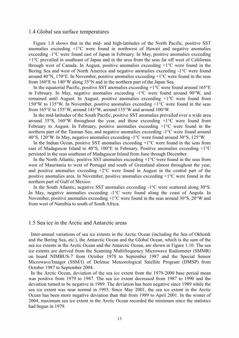
1.4 Global sea surface temperatures Figure 1.8 shows that in the mid- and high-latitudes of the North Pacific, positive SST

anomalies exceeding +1°C were found in northwest of Hawaii and negative anomalies exceeding -1°C were found east of Japan in February. In May, positive anomalies exceeding +1°C prevailed in southeast of Japan and in the area from the seas far off west of California through west of Canada. In August, positive anomalies exceeding +1°C were found in the Bering Sea and west of North America and negative anomalies exceeding -1°C were found around 40°N, 170°E. In November, positive anomalies exceeding +1°C were found in the seas from 160°E to 140°W along 35°N and in the northern part of the Japan Sea.

In the equatorial Pacific, positive SST anomalies exceeding +1°C were found around 165°E in February. In May, negative anomalies exceeding -1°C were found around 90°W, and remained until August. In August, positive anomalies exceeding +1°C were found from 150°W to 135°W. In November, positive anomalies exceeding +1°C were found in the seas from 165°E to 155°W, around 145°W, around 135°W and around 100°W.

In the mid-latitudes of the South Pacific, positive SST anomalies prevailed over a wide area around 35°S, 160°W throughout the year, and those exceeding +1°C were found from February to August. In February, positive anomalies exceeding +1°C were found in the northern part of the Tasman Sea, and negative anomalies exceeding -1°C were found around 40°S, 120°W. In May, negative anomalies exceeding -1°C were found around 30°S, 125°W.

In the Indian Ocean, positive SST anomalies exceeding +1°C were found in the seas from east of Madagascar Island to 40°S, 100°E in February. Positive anomalies exceeding +1°C persisted in the seas southeast of Madagascar Island from June through December.

In the North Atlantic, positive SST anomalies exceeding +1°C were found in the seas from west of Mauritania to west of Portugal and south of Greenland almost throughout the year, and positive anomalies exceeding +2°C were found in August in the central part of the positive anomalies area. In November, positive anomalies exceeding +1°C were found in the northern part of Gulf of Mexico.

In the South Atlantic, negative SST anomalies exceeding -1°C were scattered along 30°S. In May, negative anomalies exceeding -1°C were found along the coast of Angola. In November, positive anomalies exceeding +1°C were found in the seas around 30°S, 20°W and from west of Namibia to south of South Africa. 1.5 Sea ice in the Arctic and Antarctic areas Inter-annual variations of sea ice extents in the Arctic Ocean (including the Sea of Okhotsk and the Bering Sea, etc.), the Antarctic Ocean and the Global Ocean, which is the sum of the sea ice extents in the Arctic Ocean and the Antarctic Ocean, are shown in Figure 1.10. The sea ice extents are derived from the Scanning Multifrequency Microwave Radiometer (SMMR) on board NIMBUS-7 from October 1978 to September 1987 and the Special Sensor Microwave/Imager (SSM/I) of Defense Meteorological Satellite Program (DMSP) from October 1987 to September 2004. In the Arctic Ocean, deviation of the sea ice extent from the 1979-2000 base period mean was positive from 1979 to 1987. The sea ice extent decreased from 1987 to 1990 and the deviation turned to be negative in 1989. The deviation has been negative since 1989 while the sea ice extent was near normal in 1993. Since May 2001, the sea ice extent in the Arctic Ocean has been more negative deviation than that from 1989 to April 2001. In the winter of 2004, maximum sea ice extent in the Arctic Ocean recorded the minimum since the statistics had begun in 1979.

14

In the Antarctic Ocean, sea ice extent didn’t show the significant tendency until 2002. Sea ice extent in the Antarctic Ocean has shown positive deviation since 2003. In the Global Ocean, sea ice extent reflects the tendency in the Arctic Ocean and it has shown negative deviation since 1996.

Figure 1.10 Interannual variations of the normalized sea ice extent in the Global Ocean, the

Arctic Ocean and the Antarctic Ocean. Thin red lines indicate the biweekly variations and thick blue lines indicate the three-year running means of them. Anomalies are departure from the 1979-2000 base period means and are normalized by the biweekly standard deviations, which makes it easy to compare these three variations.

15

2. Climate change in Japan

The Japan Meteorological Agency (JMA) performs surface meteorological observations at 153 stations in Japan (see Map2 at the end of the report). JMA also conducts oceanographic observation in the seas around Japan. The data obtained are indispensable not only for the daily weather forecasting but also for the climate monitoring. Note: In section 2.1 and 2.2, the climate of Japan is described with respect to 4 areas (northern Japan, eastern Japan, western Japan, and Nansei Islands) and 11 regions (Hokkaido, Tohoku, Kanto-Koshin, Hokuriku, Tokai, Kinki, Chugoku, Shikoku, the northern part of Kyushu, the southern part of Kyushu, and Okinawa). These areas and regions are shown in Map1 at the end of the report. 2.1 Climate of Japan In 2004, warm conditions persisted during the year. The second highest annual mean national temperature was recorded. A total of ten landfalls of typhoons (the maximum record), as well as extreme heavy rainfall due to Baiu-front, caused a number of disasters. (1) Annual Climate 1) Annual mean temperature The 2004 annual average temperature of Japan (the mean value of seventeen stations which have been little influenced by the urbanization) was +0.99°C above normal, which places 2004 as the second warmest year since 1898. The annual mean temperature of eastern Japan was +1.3°C above normal, which was the warmest record since 1946. Annual mean temperatures were more than +1°C above normal at many stations. The highest annual mean temperatures were observed at 25 stations in eastern and western Japan. 2) Annual precipitation amount Annual precipitation amounts were above normal across Japan except in Hokkaido. The annual national precipitation amount was 113% of normal. Annual precipitation amounts were more than 120 % of normal at many stations from northern to western Japan. The largest annual precipitation amount of the station was recorded at Sumoto (2323 mm) (WMO Station number 47776) and Uwajima (2305 mm)(47892). 3) Annual sunshine duration Annual sunshine durations were above normal at a large number of stations except in a part of northern Japan. In particular, more than 110% of normal was recorded over Kanto-Koshin region and in a part of eastern Japan. The longest annual sunshine durations of the stations were recorded at five stations including Kofu (47638) and Osaka (47772). (2) Winter (December 2003 to February 2004) Seasonal mean temperatures were above normal in the northern and eastern Japan and near normal in both the western Japan and Nansei Islands due to winter monsoon pattern not being frequent and occasional cold surges attacking on the southerly course. While cloudy or snowy weather were dominant in the northern Japan due to cyclones frequently passing, sunny days were dominant in the other regions, where high-pressure systems tended to cover. Seasonal precipitation amounts were below normal and seasonal sunshine durations were highly above normal except for the northern Japan.

16

(3) Spring (March 2004 to May 2004) Because of migratory anticyclones frequently covering most of Japan, warm and sunny weather was dominant from March to April. On the contrary, cloudy and rainy weather was dominant in May due to fronts and cyclones. Seasonal mean temperatures were above normal in the whole of Japan. Seasonal precipitation amounts were above normal in western Japan, the Japan Sea side of northern Japan and the Nansei Islands. Seasonal sunshine durations were below normal in northern Japan, above normal in western Japan, the Pacific side of eastern Japan, and the Nansei Islands. (4) Summer (June 2004 to August 2004) In northern, eastern and western Japan, hot and sunny weather was dominant because the subtropical high tended to cover over Japan. Six typhoons made landfall on the main islands of Japan, and typhoons brought stormy weather mainly to western Japan and the Nansei islands. Seasonal mean temperatures were above normal except in the Naisei Islands. Seasonal precipitation amounts were below normal in the Pacific side of northern and eastern Japan, and in the Japan Sea side of western Japan, and above normal in the Nansei Islands. Seasonal sunshine durations were above normal in the Pacific side of Northern Japan, and in the eastern and western Japan, and below normal in the Nansei Islands. (5) Autumn (September 2004 to November 2004) Through this autumn, warm days were dominant because the influence of cold air was weaker than normal. And cloudy and rainy days were dominant due to cyclones, fronts and typhoons frequently affecting. Four typhoons made landfall on the main islands of Japan, and brought stormy weathers and disasters mainly to eastern, western Japan and the Nansei Islands. Seasonal mean temperatures were above normal all over Japan. Seasonal precipitation amounts were above normal in the Pacific side of eastern Japan, and in western Japan. Seasonal sunshine durations were below normal in the northern Japan and the Japan Sea side of western Japan. (6) Early Winter (December 2004) Warm weather was dominant up to the middle of December, because winter monsoon pattern was little appeared. In the last 10 days, cold weather was dominant, because strong winter monsoon pattern was appeared. Monthly precipitation amounts were above normal except Japan Sea side of eastern Japan and Nansei Islands where they were near normal. Monthly sunshine durations were above normal in the Japan Sea side of eastern Japan and western Japan and below normal in the Japan Sea side of northern Japan.

17

Figure 2.1 Annual climate anomalies/ratios over Japan in 2004.

The normal is 1971-2000 average.

Ogasawara Islands

Ogasawara Islands

Ogasawara Islands

18

(a) (b)

(c) (d)

Figure 2.2 Seasonal anomalies/ratios over Japan in 2004. (a) Winter (December 2003 to February 2004), (b) Spring (March to May), (c) Summer (June to August), (d) Autumn (September to November) The normal is 1971-2000 average.

Ogasawara Islands

Ogasawara Islands

Ogasawara Islands

Ogasawara Islands

Ogasawara Islands

Ogasawara Islands

Ogasawara Islands

Ogasawara Islands

Ogasawara Islands

Ogasawara Islands

Ogasawara Islands

Ogasawara Islands

19

Table2.1 Number of stations where highest (largest) or lowest (smallest) records were observed in 2004 for monthly, seasonal and annual values of temperature, precipitation and sunshine duration among the 150 (temperature), 152 (precipitation), 153 (sunshine duration) stations having statistically records over 10 years.

Mean Temperature Precipitation Sunshine Duration 2004

Highest Lowest Largest Smallest Longest Shortest

January February

0 3

1 0

1 3

6 1

2 39

0 0

Winter (December 2003 to February 2004)

6 0 0 1 15 0

March April May

0 4 5

0 0 0

0 0 15

5 3 0

0 34 1

0 0 4

Spring (March to May) 0 0 3 2 1 0

June July August

36 14 0

0 0 0

0 0 3

2 7 1

1 2 0

0 0 0

Summer (June to August) 21 0 0 2 1 0

September October November

0 1 44

0 0 0

1 32 0

1 3 2

0 0 14

5 0 0

Autumn (September to Novemver)

14 0 16 0 0 1

December 24 0 11 0 2 0

Annual amount 39 0 2 0 5 0

20

2.2 Major meteorological disasters Meteorological disasters in 2004 are mainly caused by heavy rains in the late of rainy

season and many typhoon landings, and figures of disasters are that 326 people being killed or missing, 90,791 houses damaged or destroyed, 170,654 houses flooded, and the total agricultural damage amounted to JPY 287.48 billion. Fatalities over 300 were the largest number since 1993, and other figures (as of February 21, 2005) were the new records in 2000’s.

Major meteorological disasters in 2004 and their causes are summarized in table 2.2. Table 2.3 shows the damage of the meteorological disaster from 2000 to 2004.

(1) Strong wind and Sea waves (18-21 April)

An extra-tropical cyclone system proceeded from the Japan sea to Sea of Okhotsk and developed severely. The cyclone system brought a storm around northern Japan. There was a local gust and strong rain in the passage of a cold front. A total of 5 people were killed or missing and 129 houses were destroyed. The agricultural damage amounted to JPY 0.04 billion. (2) Heavy rainfall (12-14 May)

The extra-tropical cyclone system accompanying an active front moved from central China to the Japan Sea, which caused heavy rain in western Japan. Two houses were destroyed and 1,636 houses were flooded above and below the floor level. (3) TY0406 (18-25 June)

Typhoon DIANMU moved northward over the sea east of Okinawa and landed in the eastern part of Shikoku. The typhoon passed through the Kinki region to the Japan sea, where it became an extra-tropical cyclone. After that it moved toward the vicinity of Hokkaido. Very strong wind was observed around the center of the typhoon, and heavy rain was observed on the Pacific Ocean side from Kyushu to the Kanto region. A total of 5 people were killed or missing and 171 houses were destroyed. The agricultural damage amounted to JPY 6.85 billion. (4) Heavy rainfall (12-20 July)

From the night of the 12th to the 13th July the seasonal rain front extending from the Japan Sea to the southern part of Tohoku region was activated. The torrential of rain hit around Chuetsu area in Niigata Prefecture and Aizu area in Fukushima Prefecture. In Niigata and Fukushima Prefectures, 16 people were killed or missing, 5,518 houses were destroyed and 8,394 houses were flooded above and below the floor level. The agricultural damage amounted to JPY 23.14 billion. (5) Heavy rainfall (17-21 July)

From the night of the 17th to the 18th July the seasonal rain front slowly moved southward in Hokuriku region and heavy rain was observed in the Fukui Prefecture and Gifu Prefecture. In the whole country, mainly in Fukui Prefecture, a total of 5 people were killed or missing, 409 houses were destroyed and 13,950 houses were flooded above and below the floor level. The agricultural damage amounted to JPY 20.14 billion. (6) TY0410(28 July-2 August)

After landing in Shikoku region, Typhoon NAMTHEUN moved to the Japan Sea through Chugoku region. Heavy rain was observed on the Pacific Ocean side of eastern Japan and in

21

western Japan; at several stations, the total precipitation amount was above 1,000mm. Three people were killed or missing, 89 houses were destroyed and 2,441 houses were flooded above and below the floor level. The agricultural damage amounted to JPY 4.36 billion. (7) TY0415 (16-20 August)

Typhoon MEGI moved from south of Okinawa to the Japan Sea through the East China Sea and the Tsushima Channel, and it landed in the northern part of Tohoku region. Around Kyushu and Shikoku regions, heavy rain and strong wind were observed on the Japan Sea side. Twelve people were killed or missing, 506 houses destroyed and 2,788 houses flooded above and below the floor level. The agricultural damage amounted to JPY 34.02 billion. (8) TY0416 (26 August-2 September)

Typhoon CHABA landed in Kyushu region with its strong power. It proceeded from Chugoku region to the Tsugaru Channel through the Japan Sea and passed through Hokkaido. In the Seto Inland Sea coastal area, the highest tide level was recorded and caused large damage. Totally, 17 people were killed or missing, 8,547 houses were destroyed and 46,761 houses were flooded above and below the floor level. The agricultural damage amounted to JPY 31.38 billion. (9) Heavy rainfall (3-6 September)

A front stayed along the south coast of Honshu, which brought a heavy rain from Tokai region to the southern part of Kanto region. In the whole country, one person was killed, 3 houses were destroyed and 2,384 houses were flooded above and below the floor level. (10) TY0418 (4-10 September)

Typhoon SONGDA passed through Okinawa Island with its strong power. After it passed through the northern part of Kyushu, it moved through the Japan Sea and the sea west of Hokkaido to the Soya Channel. In Okinawa, Kyushu, Chugoku Hokkaido regions maximum instantaneous wind speed above 50m/s was observed. A storm surge occurred in the coastal area of Seto Inland Sea and on the Japan Sea side. In the whole country, 46 people were killed or missing, 53,182 houses were destroyed and 8,166 houses were flooded above and below the floor level. The agricultural damage amounted to JPY 94.84 billion. (11) TY0421 (24-30 September)

Typhoon MEARI passed the Nansei Islands and proceeded to Kyushu, Shikoku, Kinki, Hokuriku and Tohoku regions. There was a heavy rain in Shikoku and Kinki regions, especially in Kii Peninsula. In the whole country, 27 people were killed or missing, 2,852 houses were destroyed and 19,116 houses were flooded above and below the floor level. The agricultural damage amounted to JPY 13.26 billion. (12) TY0422 (7-10 October)

After Typhoon MA-ON landed in Tokai region, it passed through Kanto region. It brought a heavy rain from the southern part of Tokai region to Kanto region with severe wind around the typhoon center. In the whole country, eight people were killed or missing, 4,991 houses were destroyed and 4,777 houses were flooded above and below the floor level. The agricultural damage amounted to JPY 3.86 billion. (13) TY0423 and Front (17-22 October)

Typhoon TOKAGE passed through the Nansei Islands and landed in Shikoku region maintaining strong power. It proceeded to Kinki, Tokai and Kanto regions. The large area

22

from the Nansei Islands to Kanto region was caught in a storm, a heavy rain and high sea waves. There were a lot of river overflows, landslides. In the whole country 97 people were killed or missing, 18,794 houses were destroyed and 54,951 houses were flooded above and below the floor level. The agricultural damage amounted to JPY 44.53 billion. The number of dead and missing persons by this typhoon became the most since 1989. (14) Heavy rainfall (11-12 November) Moist air flowing to front staying along the south coast of Honshu caused a heavy rain on the Pacific Ocean side from Kyushu to Kanto region. In particular, there was large damage in Shizuoka Prefecture. In the whole country, one person was killed, four houses were destroyed and 1,083 houses were flooded above and below the floor level. The agricultural damage amounted to JPY 0.1 billion. (15) Strong wind and Sea waves (4－6 December)

An extra-tropical cyclone system developed rapidly and passed through Japan, which caused storms and heavy rain over the whole country. Six people were killed or missing, 865 houses were destroyed, and 288 houses were flooded above and below the floor level. The agricultural damage amounted to JPY 1.21 billion. Table 2.2 Major meteorological disasters in Japan in 2004

Damage Type

Date

Region

Fatalities

Houses destroyed

Houses flooded

AgriculturalProduction

(billion JPY)

Strong wind, Sea waves 4.18～4.21 Hokkaido～Kyushu 5 129 0.04

Heavy rainfall 5.12～5.14 Kyushu～Kinki 2 1,636

TY0406(DIANMU) 6.18～6.25 Hokkaido～Kyushu 5 171 29 6.85

Heavy rainfall 7.12～7.20 Niigata, Fukushima 16 5,518 8,394 23.14

Heavy rainfall 7.17～7.21 Chubu, Tohoku (especially Fukui)

5 409 13,950 20.14

TY0410(NAMTHEUN) 7.28～8.2 Kyushu～Kanto 3 89 2,441 4.36

TY0415(MEGI) 8.16～8.20 Hokkaido～Kyushu (except Kanto and Tokai)

12 506 2,788 34.02

TY0416(CHABA) 8.26～9.2 Hokkaido～Kyushu 17 8,547 46,761 31.38

Heavy rainfall 9.3～9.6 Tokai～Kanto 1 3 2,384

TY0418(SONGDA) 9.4～9.10 Hokkaido～Kyushu 46 53,182 8,166 94.84

TY0421(MEARI), Front 9.24～9.30 Tohoku～Kyushu 27 2,852 19,116 13.26

TY0422(MA-ON), Front 10.7～10.10 Tohoku～Kyushu 8 4,991 4,777 3.86

TY0423(TOKAGE), Front

10.17～10.22 Tohoku～Kyushu 97 18,794 54,951 44.53

Heavy rainfall 11.11～11.12 Kyushu～Kanto 1 4 1,083 0.1

Strong wind, Sea waves 12.4～12.6 Hokkaido～Kyushu (except Okinawa)

6 865 288 1.21

Total 326 97,791 170,654 287.48

Note) This table summarizes meteorological disasters reporting more than five peoples dead or missing, more than 1,000 houses flooded and more than JPY 10 billion agriculture damages. “Fatalities” includes persons missing. Total also includes any meteorological disasters other than listed above.

23

Table 2.3 Change of the amount of damages caused by meteorological disasters in Japan

Damage

Year Fatalities Houses destroyed Houses flooded

Agricultural production(billion JPY)

2000 63 1,405 82,290 42.97 2001 110 1,782 12,856 52.00 2002 81 2,914 15,918 56.05 2003 132 3,120 16,164 277.90 2004 326 97,791 170,654 287.48

2.3 Surface temperature and precipitation

Long-term changes in surface temperature and precipitation are studied with observational

records in Japan since 1898. The meteorological stations used for deriving annual mean surface temperature and

precipitation are listed in Table 2.4. JMA selected 17 stations for calculating long-term trends of temperature, which are considered not much influenced by urbanization and have continuous records since 1898. 51 stations were selected for calculating precipitation, which have continuous records since 1898.

In 2004, the mean surface temperature in Japan is estimated to be +0.99°C above normal (1971–2000 average) , and was the second highest after 1990 in the last 107 years.

Temperature anomaly has been rising at a rate of about 1.0°C per 100 years since 1898, however there are large short-term variations (Figure 2.3). It is likely that the temperature rise in Japan was caused by human activities, particularly the emission of greenhouse gases. The temperature rise may slightly be influenced by the urbanization even for these 17 stations. In particular, the temperature has rapidly increased since the late 1980s. This tendency is almost the same as that of the worldwide temperatures described in Section 1.2.

The annual precipitation ratio to normal (1971–2000 average) in 2004 was 113%, and was above normal (1971–2000 average) for two years. The precipitation is decreasing in the long run, but it seems that the fluctuations have gradually become larger (Figure 2.4). Japan received relatively large amount of rainfall till 1920s and around 1950. Table2.4 Observation stations for calculating surface temperature anomalies and precipitation in Japan.

Observation stations

Temperature (17 stations)

Abashiri, Nemuro, Suttsu, Yamagata, Ishinomaki, Fushiki, Nagano, Mito, Iida, Choshi, Sakai, Hamada, Hikone, Miyazaki, Tadotsu, Naze and Ishigakijima

Precipitation (51 stations)

Asahikawa, Abashiri, Sapporo, Obihiro, Nemuro, Suttsu, Akita, Miyako, Yamagata, Ishinomaki, Fukushima, Fushiki, Nagano, Utsunomiya, Fukui, Takayama, Matsumoto, Maebashi, Kumagaya, Mito, Tsuruga, Gifu, Nagoya, Iida, Kofu, Tsu, Hamamatsu,Tokyo, Yokohama, Sakai, Hamada, Kyoto, Hikone, Shimonoseki, Kure, Kobe, Osaka, Wakayama, Fukuoka, Oita, Nagasaki, Kumamoto, Kagoshima, Miyazaki, Matsuyama, Tadotsu, Tokushima, Naze, Ishigakijima, Naha

24

Figure 2.3 Annual surface temperature anomalies from 1898 to 2004 over Japan.

The blue bars indicate anomalies against normal (1971–2000 average) averaged of the 17 stations. The red line indicates 5-year running mean, and the green line indicates long-term trend.

70

80

90

100

110

120

130

1890 1900 1910 1920 1930 1940 1950 1960 1970 1980 1990 2000 2010

Year

Rat

io(%

)

70

80

90

100

110

120

130

Figure 2.4 Annual precipitation ratios from 1898 to 2004 over Japan.

The blue line indicates annual precipitation ratios to normal (1971–2000 average) averaged of the 51 stations. The red line indicates 5-year running mean.

2.4 Tropical storms

In 2004, twenty-nine tropical cyclones with maximum winds of 17.2 m/s or higher formed

in the western North Pacific. Nineteen of them tracked in the areas within 300 km from the Japanese archipelago and ten of them made landfall over Japan. Figure 2.5 shows tracks of tropical cyclones in 2004. The characteristics of tropical cyclone activities in the western North Pacific in 2004 are described as follows. The number of tropical cyclone formation was 29, of which number is within the normal. However, the number of tropical cyclone approach and landfall on Japan were 19 and 10, respectively, both of which are the greatest number on record since 1951. The normal number of approach and landfall are 10.8 and 2.6, respectively.

25

Figure 2.6 shows numbers of tropical cyclones which formed in the western North Pacific, approached to and landed on Japan since 1951. Although these numbers have shown variations with different time scales, no significant long-time trends have been seen. The number of tropical cyclone formation had its maximum in the mid-1960s and the beginning of the 1990s and its minimum in the mid-1970s. Note: A tropical storm is defined as a tropical cyclone formed in the western North Pacific with maximum winds of 17.2 m/s or more.

0

10

20

30

40

50

60

100

110

120

130140

150

160

170

0

10

20

30

40

50

60

　 Typhoon Tracks　 Jan.-Dec. 2004

01

0302

04

05

06

07

09

1011

08

12

13

14

14

15

16

17

18

19

20

21

04

02

03

01

05

08

07

06

09

10

11

12

13

15

16

17

18

19

20

21

22

22

23

23

24

24

25

25

2626

27

27

28

28

29

29

0

10

20

30

40

50

60

100

110

120

130140

150

160

170

0

10

20

30

40

50

60

　 Typhoon Tracks　 Jan.-Dec. 2004

0

10

20

30

40

50

60

100

110

120

130140

150

160

170

0

10

20

30

40

50

60

　 Typhoon Tracks　 Jan.-Dec. 2004

0101

03030202

0404

0505

0606

0707

0909

10101111

0808

1212

1313

1414

1414

1515

1616

1717

1818

1919

2020

2121

0404

0202

0303

0101

0505

0808

0707

0606

0909

1010

1111

1212

1313

1515

1616

1717

1818

1919

2020

2121

2222

2222

2323

2323

2424

2424

2525

2525

26262626

2727

2727

2828

2828

2929

2929

Figure 2.5 Tracks of tropical cyclones in 2004. Solid lines are tracks of tropical storms. Dashed lines are tracks of tropical cyclones with maximum wind less than 17.2m/s or extratropical cyclones. Circled numbers next to tracks indicate domestic identification numbers of tropical storms adopted in Japan.

26

Formed

Approached

Landed

0

10

20

30

40

1950 1960 1970 1980 1990 2000

Year

Number

Figure 2.6 The number of tropical storms formed in the western North Pacific (top),

approached to Japan (mid) and landed on Japan (bottom). Solid, broken and thin lines are annual, 5-year running means and normal (1971–2000 average), respectively.

2.5 Sea surface temperatures in the western North Pacific Negative SST anomalies prevailed in east of Honshu until September 2004. Positive

anomalies prevailed in the seas from the East China Sea to south of Japan and the Japan Sea from April to August. Figure 2.7 shows that in August, positive anomalies exceeding +1°C were found in west of Kyushu and in the southern part of the Sea of Okhotsk, and negative anomalies exceeding -1°C were found around 40°N, 170°E.

Figure 2.7 also shows that annual mean SST were above normal in the seas adjacent to Japan except east of Honshu and positive annual mean anomalies exceeding +1°C were found in the northern part of the Japan Sea and off the coast of Tokai. Negative anomalies exceeding -1°C were found east of Honshu. In the Kuroshio extension area, SST were above normal throughout the year. Annual mean anomalies exceeding +0.5°C were found in the Kuroshio extension area and in the equatorial Pacific near the date line, and those exceeding +1°C were found around 35°N, 165°E.

27

Figure 2.7 Sea surface temperature (SST) anomalies (°C) in the western North Pacific.

(a) Monthly mean anomalies in August 2004 and (b) annual mean anomalies against normal (1971-2000 average) in 2004.

2.6 Sea ice in the Sea of Okhotsk

From December 2003 through May 2004, sea ice extent in the Sea of Okhotsk was normal

(normal: 30-year average from 1970/1971 to 1999/2000) from early December to early January and below normal from middle January to late May (Figure 2.8).

Sea ice extent recorded its maximum of 109.91×104km2, which is smaller than the normal annual maximum (122.83×104km2), on 10 March. This indicates that about 70% of the sea of Okhotsk was covered with sea ice. Accumulated sea ice extent, which is the sum of every 5-day sea ice extent from December to May and used as an index of the magnitude of sea ice extent in the current sea ice season, was below normal for the first time in seven years since 1997 (Figure 2.9).

(a)

(b)

28

Figure 2.8 Seasonal variations of sea ice extent from December 2003 to May 2004 in the Sea

of Okhotsk. The normal is 30-year average from 1970/1971 to 1999/2000.

Figure 2.9 Interannual variations of sea ice extent (blue bar) and its annual accumulation (red

bar) in the Sea of Okhotsk. 2.7 Sea level trend around Japan

The time series of annual mean sea level observed from 1970 to 2004 at 13 tide gauge

stations (Figure 2.10) are shown in Figure 2.11. It indicates that the sea level around Japan has risen since the middle of 1980s. The highest values over the period were recorded during the last 6 years except at Hakodate. In 2004, compared with 2003, sea levels rose up around Japan except at Kushimoto, Aburatsu and Chichijima. Especially at Wakkanai, Kushiro, Ofunato, Mera, Hamada and Toyama, the sea levels in 2004 were highest during the last three

29

decades. Table 2.5 shows the rates of the sea level rise from 1970 to 2004. It is recognized that the sea levels have risen at most stations. The maximum rate of 9.3 mm/year is observed at Kushiro. These rates contain the effect that the sea level appears to rise or fall by the crustal movement. The effect of crustal movement is being evaluated by GPS measurements.

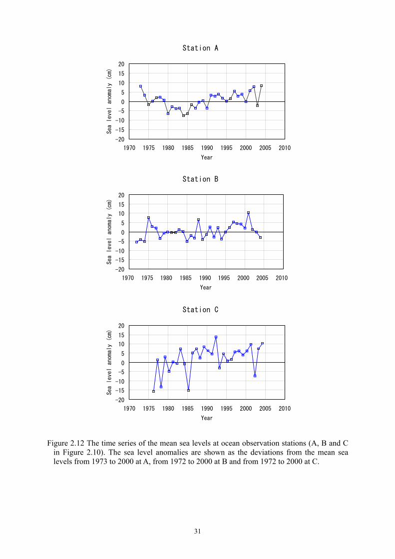
Figure 2.12 shows the long-term variation of mean sea levels at the ocean observation stations (A, B and C in Figure 2.10) in the Japan Sea, the East China Sea and south of Japanese island which are calculated from data of water temperature and salinity observed by research vessels of JMA. The characteristics of the variation are similar to the sea levels observed at adjacent tide gauge stations, Toyama, Chichijima and Naha. This indicates that the variation of sea level along the Japanese coast is mainly caused by that of sea water temperature around Japan.

Figure 2.10 Location of tide gauge stations (red circles) and oceanographic observation stations (blue squares) for monitoring the sea level

30

1965 1970 1975 1980 1985 1990 1995 2000 2005

Year

The annual mean sea levels

10cm｛Wakkanai

Abashiri

Kushiro

Hakodate

Ofunato

Mera

Chichijima

Kushimoto

Aburatsu

Naha

Nagasaki

Hamada

Toyama

Figure 2.11 The time series of the annual mean sea levels at 13 stations around Japan.

Each horizontal line shows the mean value of each station from 1970 to 2004 (from 1976 to 2004 at Chichijima). A vertical scale is equivalent to 10 cm.

Table 2.5 The rates of sea level rise (mm/year) at the stations around Japan from 1970 to 2004 (from 1976 to 2004 at Chichijima).

Wakkanai Abashiri Kushiro Hakodate Ofunato Toyama Mera

2.7 2.2 9.3 -0.4 4.5 2.5 3.6

Hamada Kushimoto Nagasaki Aburatsu Chichijima Naha

2.9 3.3 2.0 2.0 5.1 1.7

31

Figure 2.12 The time series of the mean sea levels at ocean observation stations (A, B and C

in Figure 2.10). The sea level anomalies are shown as the deviations from the mean sea levels from 1973 to 2000 at A, from 1972 to 2000 at B and from 1972 to 2000 at C.

Station A

-20

-15

-10

-5

0

5

10

15

20

1970 1975 1980 1985 1990 1995 2000 2005 2010

Year

Sea level anomaly (cm)

-20

-15

-10

-5

0

5

10

15

20

1970 1975 1980 1985 1990 1995 2000 2005 2010

sea level (cm)

那覇検潮所の海面水位

海洋観測点ＢのΔＤ

Station C

-20

-15

-10

-5

0

5

10

15

20

1970 1975 1980 1985 1990 1995 2000 2005 2010

Year

Sea level anomaly (cm)

Station B

-20

-15

-10

-5

0

5

10

15

20

1970 1975 1980 1985 1990 1995 2000 2005 2010

Year

Sea level anomaly (cm)

32

3. Monitoring of greenhouse gases and ozone depleting substances The Japan Meteorological Agency (JMA) has been continuously measuring the

concentrations of greenhouse gases such as carbon dioxide (CO2) and methane (CH4) at three stations (Figure 3.1): Ryori, Minamitorishima and Yonagunijima. JMA has also carried out an observation of greenhouse gases at altitudes of 8-13km by commercial flights between Japan and Australia. Furthermore, concentrations of greenhouse gases over the ocean and in seawater are regularly monitored by JMA research vessels in the western North Pacific. Atmospheric turbidity observations are conducted at 14 stations in Japan for studying influences of aerosol on the global climate.

Such observations have been made systematically as a part of international frameworks such as the Global Atmosphere Watch (GAW) programme of the World Meteorological Organization (WMO). JMA also operates the WMO World Data Centre for Greenhouse Gases (WDCGG) to collect, archive, and distribute the data of greenhouse gases in the world. The archived data can be accessed from all over the world through the Internet (http://gaw.kishou.go.jp/wdcgg_e.html), so that the data contributes to various studies for the carbon cycle among the atmosphere, ocean, and biosphere, and for projections of global warming.

Figure 3.1 Locations map of observation stations for greenhouse gases (3 stations), direct solar radiation (14 stations), and ozone layer and UV-B radiation (5 stations).

3.1 Greenhouse gases and ozone depleting substances in the atmosphere Table 3.1 shows the global concentrations of greenhouse gases reported to the WDCGG by

2004. The global mean atmospheric CO2 concentration has been steadily increasing. The global mean of the atmospheric CH4 and N2O concentrations slightly increased. The global mean of CO concentration, which is not a greenhouse gas but affects the concentrations of greenhouse gases, also slightly increased.

33

Table 3.1 The global mean concentrations of greenhouse gases.

Atmospheric concentration Property Para- meter

Pre-industrial level

Global mean in 2003* (Growth rate from pre-industrial level）

Increase from previous year

Lifetime (year）

Radiative forcing**

(W/m2)

CO2 ~280ppm 373.7 ppm（2002） （＋33％）

+1.8 ppm 5～200 1.46

CH4 ~ 700ppb 1782 ppb （＋155％）

+5 ppb 12 0.48

N2O ~ 270ppb 317 ppb （＋17％）

+0.5 ppb 114 0.15

CO* 98ppb（2002） +5 ppb ~ 0.25 - * CO2 and CO concentrations are global mean in 2002. * * CO is not a greenhouse gas, but it affects atmospheric concentrations of greenhouse gases through various chemical reactions. *** Radiative forcing is a measure of the influence factor which alters the balance of incoming and outgoing energy in the Earth-atmosphere system, and is an index of the importance of the factor as a potential climate change mechanism. It is expressed in Watts per square meter (Wm-2).

3.1.1 Carbon Dioxide

CO2 contributes most significantly, of all greenhouse gases, to the global warming. The atmospheric concentration of CO2 has been increasing with emissions from various human activities such as combustion of fossil fuels, production of cement, and deforestation. Among them, the combustion of fossil fuels accounts for about three fourths of all the anthropogenic CO2 emission (IPCC, 2001).

Figure 3.2 shows time series of the atmospheric CO2 concentrations at three stations in the world: Ryori (Japan), Mauna Loa (Hawaii, USA), and the South Pole. Atmospheric CO2 has been observed since 1957 at the South Pole, since 1958 at Mauna Loa, and since 1987 at Ryori. The atmospheric CO2 concentration at the South Pole or Mauna Loa was about 315 ppm at the beginning and has been increasing gradually with seasonal variation. The analysis by the WDCGG shows that the globally averaged atmospheric CO2 concentration was 373.7 ppm in 2002, and it was 33% higher than the concentration in the 18th century (about 280 ppm).

34

Figure 3.2 Time series of monthly-mean atmospheric CO2 concentrations at Ryori (Japan), Mauna Loa (Hawaii, USA), and the South Pole from 1958 to 2004 based on the data from WDCGG and the Carbon Dioxide Information Analysis Center in USA.

Figure 3.3 Three-dimensional representations of the annual variations of atmospheric CO2 latitudinal distribution (concentrations (top) and growth rates (bottom)) for the period 1983-2002. The analysis is based on the data archived by the WDCGG. Figure 3.3 shows the inter-annual variations of zonally-averaged atmospheric CO2

concentrations and growth rates from 1983 to 2002 that are produced by the WDCGG using the archived data from all over the world. The CO2 concentrations are high in mid- and high latitudes in the Northern Hemisphere while they are decreasing toward southern latitudes. This latitudinal distribution of CO2 concentration is ascribed to the existence of many CO2 sources in mid- and high latitudes in the Northern Hemisphere. The seasonal variation with

35

decreasing from spring to summer and increasing from summer to the following spring is mainly due to the activity of the terrestrial biosphere. The seasonal variation is smaller in the Southern Hemisphere because the land area is small. In both hemispheres, the atmospheric CO2 concentrations are increasing year by year. The mean growth rate during 1983 - 2002 for the globe was 1.6 ppm/year.

Figure 3.4 shows monthly-mean atmospheric CO2 concentrations, deseasonalized concentrations, and growth rates at Ryori, Minamitorishima, and Yonagunijima (see Figure 3.1). The deseasonalized concentration is obtained by filtering out variations with shorter time scales than the seasonal variation. At all stations, the CO2 concentrations increase, accompanying with the seasonal variation that is caused by photosynthesis and respiration of the biosphere. The CO2 concentration at Ryori has larger seasonal variation than other two stations, because of its location at high latitude that is influenced by biosphere activity. The CO2 concentration at Yonagunijima is, in general, higher than that at Minamitorishima while they are located almost the same latitude. This reflects influences of anthropogenic emissions throughout a year and biospheric emissions from autumn to the following spring from the Asian continent that is closely located upwind of Yonagunijima. The annual mean CO2 concentrations in 2004 were 380.3 ppm at Ryori, 378.3 ppm at Minamitorishima, and 380.0 ppm at Yonagunijima. Compared with the concentrations in the previous year, CO2 increased by 1.7 ppm at Ryori, Minamitorishima and Yonagunijima.

Figure 3.4 Time series of monthly-mean atmospheric CO2 concentrations, deseasonalized concentrations (top), and growth rates (bottom) at Ryori, Minamitorishima, and Yonagunijima. The global growth rate of CO2 concentration is not constant. Figure 3.3 shows globally

higher growth rates during 1983, 1987-1988, 1994-1995, 1997-1998 and 2002. On the other hand, a negative growth rate was observed in northern high latitudes during 1992-1993. The corresponding variations of CO2 growth rates were observed at three Japanese stations as shown in Figure 3.4 and at high altitudes over the Pacific Ocean as shown in Figure 3.5.

Increases of CO2 growth rate in 1994, from 1997 to 1998, and 2002, and the following decreases are related with El Niño events. El Niño events have two opposite effects on the atmospheric CO2 concentration. During an El Niño event, suppression of CO2-rich ocean-water upwelling reduces CO2 emissions from the ocean into the atmosphere in the eastern tropical Pacific. On the other hand, warmer and drier weather caused by an El Niño

36

event strengthens CO2 emissions from the terrestrial biosphere, particularly in the tropical regions, which are caused by plant respiration, decomposition of organic soil, and depression of photosynthesis. The latter effect is more dominant than the former, which brings about a net CO2 increase in the atmosphere with several month delay (Keeling et al., 1989; Nakazawa et al., 1993; Dettinger and Ghil, 1998). Anomalously low precipitation that brought about the droughts and the frequent forest fires in Southeast Asia in 1997/1998 and the remarkable high global mean temperature in 1998 are considered to have strengthened CO2 emissions from the terrestrial biosphere (Watanabe et al., 2000).

Although the El Niño event occurred during 1992-1993, the CO2 growth rate decreased significantly during this period. The increase in absorption of CO2 into the terrestrial biosphere and the ocean, which was resulted from global cooling by the eruption of Mt. Pinatubo, brought about the growth rate decrease (Rayner et al., 1999). These inter-annual variations in CO2 growth rate can be interpreted as fluctuations of the carbon cycle that is influenced by climate. Since these fluctuations in the carbon cycle can affect climate through the global warming, it is necessary to clarify the carbon cycle system including the inter-annual variations to achieve an accurate projection of the global warming.

The Meteorological Research Institute of JMA has been carrying out the measurement of trace gases such as CO2 at altitudes of 8-13km by commercial flights between Japan and Australia in cooperation with the Japan Air Line Foundation, the Ministry of Land, Infrastructure and Transport, and the Japan Airlines. Fig 3.5 shows the time series of the atmospheric CO2 concentrations obtained by the measurement. The CO2 concentrations increase with seasonal variations like those on the surface, but the amplitudes are smaller. In the Southern Hemisphere, the variations are complicated with double peak seasonality（Matsueda et al., 2002）.

37

Figure 3.5 Time series of CO2 concentrations (dots), deseasonalized concentrations (blue dashed line), and growth rates (red solid line) averaged in each 5-degree latitudinal zone observed at altitudes of 8-13km. The data used in this analysis were collected by commercial flights between Japan and Australia.

3.1.2 Methane CH4 is the second most significant greenhouse gas after CO2, and emitted into the

atmosphere from various sources including wetlands, rice paddy field, ruminant animals, natural gas production, and biomass burning. CH4 is primarily removed from the atmosphere by photochemical reaction with hydroxyl (OH) radicals, which is a very reactive and unstable molecule.

The analysis by the WDCGG shows that the globally averaged atmospheric CH4 concentration was 1787 ppb in 2003. The concentration is almost 2.5 times as large as that before the 18th century (about 700 ppb).

38

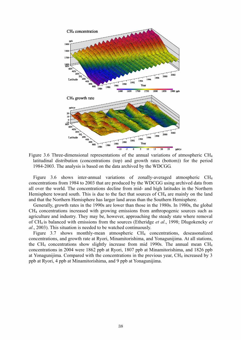
Figure 3.6 Three-dimensional representations of the annual variations of atmospheric CH4 latitudinal distribution (concentrations (top) and growth rates (bottom)) for the period 1984-2003. The analysis is based on the data archived by the WDCGG. Figure 3.6 shows inter-annual variations of zonally-averaged atmospheric CH4

concentrations from 1984 to 2003 that are produced by the WDCGG using archived data from all over the world. The concentrations decline from mid- and high latitudes in the Northern Hemisphere toward south. This is due to the fact that sources of CH4 are mainly on the land and that the Northern Hemisphere has larger land areas than the Southern Hemisphere.

Generally, growth rates in the 1990s are lower than those in the 1980s. In 1980s, the global CH4 concentrations increased with growing emissions from anthropogenic sources such as agriculture and industry. They may be, however, approaching the steady state where removal of CH4 is balanced with emissions from the sources (Etheridge et al., 1998; Dlugokencky et al., 2003). This situation is needed to be watched continuously.

Figure 3.7 shows monthly-mean atmospheric CH4 concentrations, deseasonalized concentrations, and growth rate at Ryori, Minamitorishima, and Yonagunijima. At all stations, the CH4 concentrations show slightly increase from mid 1990s. The annual mean CH4 concentrations in 2004 were 1862 ppb at Ryori, 1807 ppb at Minamitorishima, and 1826 ppb at Yonagunijima. Compared with the concentrations in the previous year, CH4 increased by 3 ppb at Ryori, 4 ppb at Minamitorishima, and 9 ppb at Yonagunijima.

39

Figure 3.7 Time series of monthly-mean atmospheric CH4 concentrations, deseasonalized concentrations (top), and growthrate (bottom) at Ryori, Minamitorishima, and Yonagunijima.

3.1.3 Nitrous Oxide Nitrous oxide (N2O) is a significant greenhouse gas, because its radiative effect per unit

mass is about 200 times than that of CO2, and it has a long lifetime (the quantity that the total amount in the atmosphere is divided by the decomposition rate per year) of about 114 years in the atmosphere. N2O is emitted into the atmosphere from soil, the ocean, use of nitrate and ammonium fertilizers, and various industrial processes. N2O is photodissociated in the stratosphere by ultraviolet radiation.

The concentration of atmospheric N2O has been slightly increasing globally. According to the analysis of the WDCGG, the global mean concentration of atmospheric N2O was 318 ppb in 2004. This concentration was about 17% higher than the concentration before the 18th century (about 270 ppb) (IPCC, 2001).

Figure 3.8 shows time series of monthly-mean N2O concentration in the atmosphere observed at Ryori. Short-term variation is very weak and no seasonal variability is observed. The annual mean N2O concentration was 319 ppb in 2003, showing still slightly increasing trend.

Figure 3.8 Time series of monthly-mean atmospheric N2O concentrations at Ryori.

3.1.4 Halocarbons Halocarbons are carbonic compounds with fluorine, chlorine, bromine, or iodine. Most of

them do not exist in the natural atmosphere but are chemically manufactured. They do not only destroy stratospheric ozone, but also warm the global atmosphere directly as greenhouse

40

gases and, at the same time, cool the lower stratosphere indirectly through ozone destruction in the stratosphere. The atmospheric concentrations of most halocarbons are less than a millionth of that of CO2. However, they contribute significantly to the global warming because their radiative effects per unit mass are several thousand times larger than that of CO2. Furthermore, the effects can last very long because of their long lifetimes in the atmosphere.

Chlorofluorocarbons (CFCs), which are compounds of carbon, fluorine, and chlorine, are important substances in halocarbons. Emissions of CFCs have been regulated by the Montreal Protocol on Substances that Deplete the Ozone Layer. Consequently, the observation by the Atmospheric Lifetime Experiment/Global Atmospheric Gases Experiment (ALE/GAGE) shows that the CFC-11 concentration was at the peak in 1993 and has declined since 1994. The CFC-12 concentration has been increasing while the growth rate has become much lower, and the CFC-113 concentration has stopped increasing since 1996 (WMO, 1999).

Figure 3.9 shows time series of monthly mean concentrations of CFC-11, CFC-12, and CFC-113 in the atmosphere observed at Ryori, indicating weak short-term variations and no seasonal variability. The CFC-11 concentration had a peak of about 280 ppt during 1993-1994 and has a decreasing trend since then. The CFC-12 concentration has almost stopped increasing for the last few years. The CFC-113 concentration indicates little change. The annual mean concentrations in 2004 were about 260 ppt for CFC-11, about 540 ppt for CFC-12, and about 80 ppt for CFC-113.

Hydrochlorofluorocarbons (HCFCs), hydrofluorocarbons (HFCs), and perfluorocarbons (PFCs), which are used as substitutes for CFCs, have been increasing in the atmosphere. For example, the observation by the Climate Monitoring and Diagnostics Laboratory (CMDL) in the National Oceanic and Atmospheric Administration (NOAA) showed that the total chlorine concentration from major three HCFCs was 205 ppt in the middle of 2003. The HFC-134a concentration was 25.5 ppt in 2003, and the increasing rate was 4.3ppt/year from 2002 to 2003 (CMDL, 2003). CMDL also reported that the concentration of SF6, which is an effective gaseous dielectric and enclosed in electrical equipment, was 5.23 ppt at September of 2003 and had been increasing linearly by 0.2 pptv/year since 1996. HFCs, PFCs, and SF6 are the greenhouse gases, as well as CO2, CH4, and N2O, which are subject to the Kyoto Protocol to the United Nations Framework Convention on Climate Change.

Figure 3.9 Time series of monthly-mean concentrations of atmospheric CFC-12 (top), CFC-11 (middle), and CFC-113 (bottom) at Ryori.

41

3.1.5 Carbon Monoxide Sources of carbon monoxide (CO) are emissions from industrial and agricultural

combustion and production from oxidation of hydrocarbons including methane. It is mainly removed through a reaction with OH radicals in the atmosphere. CO is not a greenhouse gas in itself because it hardly absorbs infrared radiation from the earth’s surface. However, CO is controlling many greenhouse gases through a reaction with OH radicals as well as a precursor of tropospheric ozone (Daniel and Solomon, 1998).

The analysis by the WDCGG shows that the globally averaged atmospheric CO concentration was about 98 ppb in 2002. The analysis of ice cores shows that the concentration of CO in Antarctica, approximately 50 ppb, indicates little change for the last 2000 years (Haan and Raynaud, 1998). They also suggested that the concentration of CO in Greenland had been about 90 ppb before the middle of 19th century, and had gradually increased to about 110 ppb in 1950.

Figure 3.10 shows the annual variations of latitudinal distribution of CO concentration and growth rate for the period 1992-2002. The seasonal cycle with high concentrations from winter to spring and low concentrations in summer is obvious. The concentrations are high in northern mid-latitudes and low in Southern Hemisphere, indicating that the major sources are in the northern mid-latitudes and the concentration decreases with transporting to the equatorial area that is a major sink region of CO.

The concentrations from the equatorial area to the northern mid-latitudes had enhanced from 1997 to 1998. The large-scale biomass burning in Indonesia in 1997 and forest fires in Siberia from summer to autumn in 1998 influenced the enhancement of CO (Novelli et al., 2003).

Figure 3.10 Three-dimensional representations of the annual variations of atmospheric CO latitudinal distribution (concentrations (top), and growth rates (bottom)) for the period 1992-2002 This analysis is based on the data archived by the WDCGG .

42

Figure 3.11 shows time series of monthly-mean atmospheric CO concentrations and deseasonalized concentrations at Ryori, Minamitorishima, and Yonagunijima. The concentrations show seasonal variations with a peak from winter to early spring and a depression in summer. An increase in the CO concentration was seen from 1997 to 1998, suggesting influences of the forest fires in Indonesia and Siberia. The annual mean concentrations in 2003 were 175 ppb at Ryori, 132 ppb at Minamitorishima, and 162 ppb at Yonagunijima. The lifetime of CO in the atmosphere is 2 to 3 months, resulting in large spatial and temporal variations that depend on the local emissions. The east coast of the Asian continent is considered as one of the active CO emission areas due to less efficient combustion from burning of biofuel (Wang et al., 2001). The concentration at Yonagunijima is higher than that at Minamitorishima while both stations locate almost in the same latitudinal zone, because Yonagunijima is frequently influenced by the CO emissions in the Asian continent. High CO concentrations at Yonagunijima in 2003 and early 2004 are also supposed to be the influence of the frequent air flow from the Asian continent.

Figure 3.11 Time series of monthly-mean atmospheric CO concentrations and deseasonalized concentrations at Ryori, Minamitorishima, and Yonagunijima.

3.1.6 Tropospheric Ozone Most part of atmospheric ozone (O3) exists in the stratosphere and shields life on earth by

absorbing harmful ultraviolet solar radiation. Tropospheric ozone (O3) takes under 10% in mass, but high concentration of ozone does harm to human bodies, for example, stimulates to human eyes or gives pain to throats, and also withers plants. So the ozone regulation in Japan is below 60 ppb for an hourly mean. Furthermore, tropospheric O3 acts as an important greenhouse gas, because it also has strong absorption bands in infrared wavelength not only in ultraviolet wavelength. Tropospheric ozone is also a chemically reactive gas and produces OH radicals that control atmospheric concentrations of many greenhouse gases such as CH4 through chemical reactions.

Tropospheric ozone is produced from photochemical oxidation of CH4, CO, and non-methane hydrocarbons (NMHCs) under the nitrogen oxides (NOx) rich environment. O3 is removed by reactions with hydrogen oxides (HOx, i.e., HO2 and OH). In mid- and high latitudes, ozone is transported from the stratosphere down to the troposphere, and also destroyed on the earth’s surface. The concentration varies significantly with locations, altitudes, and seasons.

Figure 3.12 shows time series of monthly-mean surface ozone concentrations and deseasonalized concentrations at Ryori, Minamitorishima, and Yonagunijima. The concentration at Ryori has slightly increased since the beginning of observation in 1990. The concentration at Minamitorishima had decreased but has turned to increase for these two or three years. Tropospheric O3 concentration changes locally, so it is very difficult to clarify the reason of such variability. The concentrations usually show seasonal variations with a peak

43

from spring through early summer and a depression in midsummer, because in midsummer, OH radical concentrations which reduce O3 concentration increase as water vapor increases with increasing temperature. While Yonagunijima is located in the same latitudinal zone as Minamitorishima, the concentration at Yonagunijima is usually higher than that at Minamitorishima. In the eastern region of China, the peak of the monthly mean ozone concentrations is observed in autumn; the maximum at the Changjiang River Delta exceeds 60 ppb (Chameides et al., 1999). The concentrations at Yonagunijima are higher than those at Ryori from autumn to early spring. The ozone-rich air masses are supposed to be transported from the Asian continent to Yonagunijima. The annual mean concentrations in 2004 were 41 ppb at Ryori, 31 ppb at Minamitorishima, and 42 ppb at Yonagunijima.

Figure 3.12 Time series of monthly-mean surface ozone concentrations and deseasonalized concentrations at Ryori, Minamitorishima, and Yonagunijima.

3.2 Oceanic Carbon Dioxide It is important to evaluate how much the anthropogenically released CO2 is taken up by the

ocean in order to predict future concentration of atmospheric CO2 and its resultant global warming. On a global scale, it is estimated that the ocean absorbs CO2 at about 2 PgC (2× 1015 g carbon) per year (IPCC, 2001). On a regional scale, however, the amount of oceanic CO2 uptake differs from place to place. Besides, some regions such as the equatorial Pacific emit CO2 and other regions change its role as a sink or source for atmospheric CO2 depending on seasons. These geographical inhomogeneity and seasonal variations of the behavior of the ocean make it difficult to estimate oceanic CO2 uptake. It is necessary to evaluate the absorption or emission amount of CO2 quantitatively for each region and season in order to reduce the uncertainty of the estimate. JMA has conducted ship observations for greenhouse gases (CO2, CH4, CFCs and N2O) in the sea surface air and in the surface seawater along the fixed line in the western North Pacific using the research vessels Ryofu Maru and Keifu Maru.

Figure 3.13 shows the long-term variations of atmospheric and oceanic CO2 concentrations in January and February averaged between 3°N and 30°N along 137°E. In this region, the concentration of oceanic CO2 is lower than that of atmospheric CO2, suggesting that the ocean acts as a sink for atmospheric CO2 in winter. The concentrations of both the atmospheric and oceanic CO2 in this region have increased at the mean growth rate of about 1.6 ppm/year from 1981 to 2004. The oceanic CO2 has larger interannual variability compared with the relatively monotonic increase in the atmospheric CO2. The rapid mixing of air forms uniform atmospheric CO2 concentration, whereas oceanic CO2 concentration varies largely year by year, depending on the different conditions of the advection of surface water and the mixing between surface layer water and subsurface layer water.

44

Figure 3.13 Time series of the concentrations of atmospheric and oceanic CO2 along 137°E

(the average of 3°N–30°N) in winter (January–February) from 1981 to 2004 and the map of observation lines. Figure 3.14 shows the time series of atmospheric and oceanic CO2 concentrations at

156°E-165°E of the equatorial Pacific from 1996 to 2004. The oceanic CO2 concentration in the region is usually higher than the atmospheric CO2 concentration. However, the difference between the concentrations of atmospheric and oceanic CO2 was small in autumn 1997 and after winter 2002. The Southern Oscillation Index was negative during these periods (Figure 1.7) and the easterly trade winds over the equatorial Pacific were weaker than usual. The small difference between the atmospheric and oceanic CO2 concentrations is considered to be caused by the eastward advection of surface warm water with low CO2 concentration into this region and the weak upwelling of CO2-rich water from a subsurface layer.

Figure 3.14 Time series of the concentrations of atmospheric and oceanic CO2 in the equatorial Pacific (the average of 156°E–165°E) from 1996 to 2004. Red areas represent periods of El Niño events and blue areas represent periods of La Niña events.

45

In the subtropical western North Pacific, the concentration of oceanic CO2 is closely correlated with the sea surface temperature (Inoue et al., 1995). Using the empirical interpolation method based on this high correlation, the concentration of oceanic CO2 and the air-sea partial pressure difference of CO2 can be estimated for the seasons and the regions of no observed CO2 data (Murata et al., 1996). Furthermore, with the calculated air-sea partial pressure difference of CO2 and the monthly mean wind speed distribution over the ocean, air-sea CO2 exchange flux can be estimated. Figure 3.15 shows the time series of annual net CO2 flux from 1996 to 2003 in the region (11°N-30°N and 130°E-165°E) that occupies 2.7% area of the global ocean. This region acts as a source in summer and a sink in winter for atmospheric CO2. On a yearly base, however, this region acts as a net sink, because the absorption amount of CO2 in winter is estimated to be greater than the emission amount in summer. The estimated annual net flux fluctuated between 30 TgC (30 x 1012 g carbon) and 85 TgC per year during the period and was 67 TgC per year in 2003. This amount in 2003 is equal to about 3% of the net absorption amount of the global ocean.

Figure 3.15 Inter-annual variation of net air-sea CO2 flux in the subtropical region of the western North Pacific (11°N-30°N and 130°E-165°E) from 1996 to 2003. The unit is teragram (1012 gram) of carbon per year and positive values mean uptake by the ocean. The gas transfer formulation is based on Tans et al. (1990), and the gas transfer coefficient is calculated using monthly-mean surface-wind speed estimated from objective-analysis data of the Japan Meteorological Agency.

3.3 Aerosols Small particles floating in the atmosphere are called aerosols. Aerosols directly and

indirectly affect climate. Directly, aerosols decrease the global temperature because it scatters and absorbs solar radiation. On the other hand, it also warms the atmosphere by absorbing and reemitting infrared radiation from the earth’s surface. Indirectly, the aerosol changes the characteristics of cloud by acting as cloud condensation nuclei (CCN), resulting in the change of the planetary albedo. While the large uncertainties still remain in contribution of these opposite effects to climate change, an increase in the aerosol amount is estimated to decrease the surface temperature on a global scale.

3.3.1 Turbidity coefficient by direct solar-radiation measurement

JMA has been monitoring direct solar-radiation at 14 stations in Japan to obtain the Feussner-Dubois turbidity coefficient that is information on atmospheric turbidity. The turbidity coefficient is an index of impurity of the atmosphere caused by the turbid constituents such as aerosol, water vapor, ozone, and CO2. The turbidity coefficient is

46

expressed as the ratio of solar radiation extinction in the observed atmosphere to that in the ideal atmosphere that includes no such impurity. A larger value means that more turbid constituents are loaded in the atmosphere.

Figure 3.16 shows time series of Feussner-Dubois turbidity coefficient at Nemuro, Matsumoto, Shionomisaki and Ishigakijima (see Figure 3.1) in 2004. At the first three stations, the turbidity coefficients in summer are larger than that in winter mainly due to the seasonality of water vapor. Ishigakijima is an island that have a less seasonal variation of water vapor, and the turbidity coefficient in spring was larger mostly due to the influence of the aeolian dust, which is called “yellow sand” and frequently comes from the Asian continent in spring.

Figure 3.16 Time series of the Feussner-Dubois turbidity coefficient at Nemuro, Matsumoto, Shionomisaki and Ishigakijima in 2004. The daily minimum are selected in which the hourly mean meets following three condition: sun is shining, solar elevation is high (optical air mass ≤ 2.5), and the difference between maximum and minimum of direct solar radiation within 5 minutes is less than 0.03 kW/m2. A solid line in the figure indicates smoothed monthly mean values at local noon for 1971-2000. Figure 3.17 shows a yearly variation of the Feussner-Dubois turbidity coefficient from 1961

to 2004 in which the shorter variations than seasonal variation are filtered out. In this analysis, the monthly minimum values averaged over 14 stations in Japan are used to avoid influences of water vapor and severe dust events that varies largely day by day. The enhancements of Feussner-Dubois turbidity coefficient in the periods of 1982–1985 and 1991–1993 are due to the eruptions of Mt. El Chichon (Mexico) in 1982 and Mt. Pinatubo (Philippines) in 1991, respectively. Both eruptions put a huge volume of volcanic ash and SO2, which is a precursor of sulfate aerosol, into the stratosphere. At present, the Feussner-Dubois turbidity coefficient has returned to the level before the eruption of Mt. El Chichon.

47

Figure 3.17 Smoothed time series of the Feussner-Dubois turbidity coefficient from 1961 to 2004 averaged over 14 stations in Japan. The monthly minimum values are used in order to minimize influences of water vapor and severe dust events, and the variations with shorter time scales than seasonal variation are filtered out.

3.3.2 Aerosol optical depth observed with sunphotometers JMA has been carrying out aerosol optical depth (AOD: an index of the atmospheric

turbidity by aerosols) observation with sunphotometer three times a day, 9, 12, 15 JST (Japan Standard Time) at Ryori, 8, 11, 14 JST at Minamitorishima, 10, 13, 16 JST at Yonagunijima. The data are not obtained when clouds cover the sun at the time of observation.

Figure 3.18 shows the time series of aerosol optical depth and Ångström exponent (α: an index of aerosol size distribution, the larger value indicates dominant distribution of smaller size aerosols) observed at Ryori, Minamitorishima and Yonagunijima in 2004. The AOD at Minamitorishima kept lower values through the year. On the other hand, the variations of AOD were relatively large at Ryori and Yonagunijima. These large variations of the two stations might be ascribed to the influence of aeolian dust (yellow sand), biomass burning, and anthropogenic pollutants from the Asian continent.

Figure 3.18 The time series of aerosol optical depth (AOD) (blue) at 500nm and Ångström exponent (α) (red) observed at Ryori, Minamitorishima and Yonagunijima in 2004.

48

Figure 3.19 shows the successive variations of monthly-averaged AOD at 500nm from 1998 to 2004, observed at Ryori, Minamitorishima and Yonagunijima. It must be noted that the monthly-averaged data may not represent the averaged aerosol condition of the month, if adopted number is very low after data selections especially in cloudy seasons.

At Ryori, the AOD has maximums in spring or summer. The influence of aeolian dust causes the spring maximums. Additionally, the air pollutants transported from the Asian continent might be superposed in spring. As shown in the model calculation by Takemura et al.(2002; 2003), the effects on aerosol optical properties originated from aeolian dust and continental pollutants are comparable. At Minamitorishima, the AOD has lower values than that of other two stations through the year. It might be due to the far distance from Minamitorishima to aerosol source regions in the continent. The Ångström exponents are relatively smaller than Ryori and Yonagunijima. This indicates that larger particles dominate at Minamitorishima as compared with Ryori or Yonagunijima. The AOD at Minamitorishima has maximums in spring and the minimums in winter. The long distance transportation of aeolian dust or air pollutants from the Asian continent is one of the reasons for the larger AOD in spring as compared with yearly average value of Hawaii (Smirnov et al., 2002)

At Yonagunijima, the AOD usually has maximums in winter or spring, and minimums in summer or autumn. The reason for the maximums in winter or spring is likely the influences of outflow from the Asian continent. Tsutsumi et al., (2004) showed that the large AOD in Yonagunijima in spring 2002 was the result of influences of air pollutants of the Asian continent or smokes from biomass burnings in southeast Asia. The seasonal variation in Yonagunijima is consistent with the result of Tsutsumi et al. (2004).

Figure. 3.19 The time series of monthly averaged AOD at 500nm and Ångström exponent during from 1998 to 2004, observed at Ryori (top), Minamitorishima (middle) and Yonagunijima (bottom), respectively.

49

3.3.3 Vertical profiles of aerosols observed by lidar system Lidar (laser radar) system is one of the remote sensing instruments that can detect the

vertical distributions of aerosol, which shoots laser light to the sky and detecting the scattered light by the atmosphere or aerosols with telescopes. Furthermore, using of scattering properties from each aerosols, lidar can distinguish between spherical aerosols like sulfates and non-spherical aerosols like aeolian dust.

Figure 3.20 shows 3-month mean aerosol vertical profiles (scattering ratio) in 2004. The vertical profiles of scattering ratio show that the aerosol amount of the stratosphere was quite less than that in the troposphere, and the aerosol amount in the troposphere had a large variability in season. The large amount of aerosol in the lower troposphere indicates that the sources of aerosols mainly exist at the earth’s surface.

In the middle troposphere, the mean aerosol amount in spring was larger than those in other seasons. The aeolian dust (yellow sand), which is transported from the Asian continent, causes this increment in spring.

Figure 3.20 Vertical profiles of three-month averaged (only clear days) scattering ratio observed with the lidar system at a wavelength of 532nm (solid line), and its standard deviations (shaded area) at Ryori in 2004. The tropospheric aerosols such as mineral dust, sulfate aerosol, and soot particles give

influence to short-term variations of the climate. In the stratosphere, the aerosols suspended for a long time possibly give significant influences on climate if volcanic eruption injects smokes or gases into the stratosphere. Lidar system is expected as one of the effective means to clarify the behavior of aerosols.

50

4. Monitoring of the ozone layer and ultraviolet B (UV-B) radiation Ozone, distributed mainly in the stratosphere (altitude of 10-50 km) or ozone layer, is

protecting the terrestrial ecosystem from harmful solar UV (ultraviolet) radiation by absorbing it. Depletion of the ozone layer has been observed over Antarctica mainly from September through November since the early 1980s. This phenomenon is called "ozone hole". The ozone hole, which appears over Antarctica under its unique meteorological conditions resulting from the Antarctic topography and polar night, is mainly caused by man-made chlorofluorocarbons (CFCs) and halons. CFCs and halons have been widely used for various purposes such as cleaning solvents, aerosol propellants, refrigerants, and fire extinguishers, with their excellent characteristics such as chemical stability, uncombustibility, innocuousness, etc. Due to their stability, however, CFCs are hardly decomposed in the troposphere and spread gradually into the stratosphere, where CFCs are decomposed into chlorine atoms that destroy ozone molecules. The ozone layer depletion, which is typically characterized by the ozone hole, is observed in both hemispheres except equatorial zone.

Ozone layer is depleted as in the following process. When CFCs reach the altitude of about 40 km in the stratosphere, solar UV radiation detaches free atomic chlorines from CFCs. The atomic chlorine, while moving in the stratosphere, reacts with and destroys ozone (converting ozone to molecular oxygen by detaching one oxygen atom) around them, with itself changing to chlorine monoxide, which turns back to atomic chlorine again reacting with atomic oxygen and other molecules. The released atomic chlorine reacts with and destroys ozone again. These processes occur in a virtual chain reaction and destroy ozone repeatedly.

4.1 Observational results of the ozone layer 4.1.1 Global ozone layer

As for the total ozone in 2004 based on the satellite data (TOMS), negative anomalies (against monthly mean value from 1979 to 1992) generally prevailed in the southern mid-latitudes.

The global long-term trends of total ozone are shown in Figure 4.1 based on the satellite data. The decreasing trends are obvious except in the tropics, being more distinct with higher latitudes. Though not shown apparently here, the decreasing trends are large in the springtime in both hemispheres. These characteristics are due to the fact that the ozone depletion by chlorine is accelerated in the cold condition in the high-latitude stratosphere from winter through spring.

4.1.2 Ozone layer over Japan

The JMA has been carrying out total ozone observation and vertical profile observation by ozonesonde at several domestic stations and in the Antarctica since 1957 (see Figure 3.1). Total ozone variations over Japan in 2004 are shown in Figure 4.2. Monthly mean values lower than normal were seen from spring through autumn in Sapporo, and in the former half of the year in Tsukuba. Especially, the monthly mean of October in Sapporo and the monthly mean of May in Tsukuba were the lowest values among the records from the beginning of monitoring in 1958 and 1957, respectively. In Naha, the monthly mean total ozone was almost continuously higher than normal in the latter half of the year. Especially in July, October and November, the highest values among the records from the beginning of monitoring in 1974 were observed for respective months. At Minamitorishima, the monthly means of total ozone were lower than normal in the former half of the year. In the meantime, 'almost normal' indicates values within the standard deviation from the monthly mean values and 'higher/lower than normal' values are higher/lower than 'almost normal' in this section.

51

Figure 4.1 Latitudinal distribution of long-term trends in total ozone based on satellite observation. This is a change per 10 years derived from time series of total ozone averaged over every 10 degree latitudinal zone (1979-2000) by subtracting seasonal variation, effects of solar activity, etc. Vertical bars show the range of 95% confidence limit. This is derived from Merged Ozone Data produced from TOMS data and SBUV/2 data by NASA.

Figure 4.2 Monthly means of total ozone at five stations in Japan: Sapporo, Tsukuba/Tateno, Kagoshima, Naha, Minamitorishima, and Syowa Station (Antarctica). Closed circles indicate the values in 2004 and solid lines indicate normal (average over 1971-2000 but 1974-2000 in Naha and 1994-2003 in Minamitorishima) with bars of standard deviation. As for Syowa, a solid line indicates monthly mean values before the appearance of the ozone hole (1961-1980) and a dotted line indicates those after the appearance (1981-2000).

Time series of annual mean total ozone at four stations in Japan are shown in Figure 4.3. The decreasing trends in total ozone are seen at all stations except Naha, and are more remarkable at northern stations. Based on the vertical distributions of ozone concentration, the decreasing trends in the upper stratosphere are significant at all stations. These features are same in other regions.

52

Figure 4.3 Time series of annual mean total ozone at four stations in Japan. The solid lines indicate long-term trends.

4.1.3 Ozone layer over Antarctica: The ozone hole Based on TOMS data, the maximum area of the ozone hole and the ozone mass deficit in

2004 over the Antarctic region were the third lowest values in last 10 years. The ozone hole in 2004 expanded in late August, reaching the maximum in late September, and shrank rapidly in middle November, then disappeared (Figure 4.4 and 4.5).

Observation data at Syowa station in 2004 shows that total ozone was relatively high until mid-September, thus the monthly mean in August was 264 m atm-cm which is the highest value after 1989. While the total ozone value became less than 220 m atm-cm (an index of ozone hole) from mid-September through October, the total ozone increased with large variation in November. Finally, the total ozone reached around 300 m atm-cm in December. Based on ozonesonde data on October 7, 2004 when the Syowa station was located inside the ozone hole, ozone concentration was decreased to almost zero at the altitudes of 14-20 km over the Syowa station, while the degree of depletion was not so severe as in 2003 when the record-size ozone hole was observed (Figure 4.6). The reason why the ozone hole in 2004 was relatively small is interpreted that the condition for severe ozone depletion was not satisfied, i.e., a cold area of temperature less than 195K(–78°C), which is necessary for formation of polar stratospheric clouds (PSCs) that accelerate ozone depletion, rapidly shrank since September.

Figure 4.4 Total ozone distribution in the Southern Hemisphere on September 22, 2004 from TOMS data, when ozone hole area in 2004 reached an annual maximum. TOMS data were supplied by NASA.

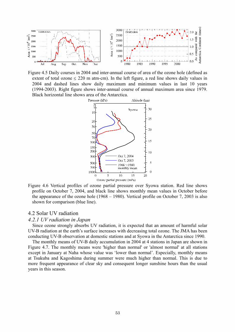
53

Figure 4.5 Daily courses in 2004 and inter-annual course of area of the ozone hole (defined as extent of total ozone ≤ 220 m atm-cm). In the left figure, a red line shows daily values in 2004 and dashed lines show daily maximum and minimum values in last 10 years (1994-2003). Right figure shows inter-annual course of annual maximum area since 1979. Black horizontal line shows area of the Antarctica.

Figure 4.6 Vertical profiles of ozone partial pressure over Syowa station. Red line shows profile on October 7, 2004, and black line shows monthly mean values in October before the appearance of the ozone hole (1968 – 1980). Vertical profile on October 7, 2003 is also shown for comparison (blue line).

4.2 Solar UV radiation 4.2.1 UV radiation in Japan

Since ozone strongly absorbs UV radiation, it is expected that an amount of harmful solar UV-B radiation at the earth’s surface increases with decreasing total ozone. The JMA has been conducting UV-B observation at domestic stations and at Syowa in the Antarctica since 1990.

The monthly means of UV-B daily accumulation in 2004 at 4 stations in Japan are shown in Figure 4.7. The monthly means were 'higher than normal' or 'almost normal' at all stations except in January at Naha whose value was ‘lower than normal’. Especially, monthly means at Tsukuba and Kagoshima during summer were much higher than normal. This is due to more frequent appearance of clear sky and consequent longer sunshine hours than the usual years in this season.

54

Figure 4.7 Monthly mean values of UV-B daily accumulation at four stations in Japan: Sapporo, Tsukuba/Tateno, Kagoshima, and Naha. Closed circles indicate the values in 2004 and solid lines indicate normal (average over 1990-2003 for Tsukuba and 1991-2003 for other stations) with bars of standard deviations. In Japan the significant trends are not seen in UV-B radiation data since 1990. This is

considered because the total ozone does not have significant trends over Japan since 1990. However, based on the observation data that shows long-term decrease of total ozone since 1970s, and the observational fact that the UV-B radiation increases with decreasing total ozone, the UV-B radiation after 1990s is estimated to be increased compared with that in 1970s. For example, at the northern station Sapporo where ozone depletion is most remarkable in Japan, an increase in UV-B radiation may be up to 8% in some months. Meanwhile, at Naha in low latitudes, a change in UV-B radiation is estimated to be insignificant due to an insignificant change in total ozone. It is reported that UV radiation is increased by 6-14% since the former 1980s at more than 10 stations in both hemispheres (WMO, 2003).

4.2.2 UV Index

It is known that excessive exposure to solar UV may influence on human health such as increasing the risk of skin cancer and cataracts. As a scale of UV radiation that shows a degree of effects on human body, erythemal UV radiation calculated by considering different effectiveness depending on wavelength is widely used. UV Index is a standardized index of erythemal UV radiation. In Japan, observed UV Index usually ranges between 0 and 12. Presently, the World Health Organization (WHO), World Meteorological Organization (WMO), United Nations Environment Programme (UNEP), etc., recommend to promote UV protecting measures using UV Index. As actual measures, it is suggested to seek shade during midday hours for UV Index larger than 3, and to avoid being outside during midday hours for UV Index larger than 8.

Daily maximum UV Index at domestic 4 stations in 2004 is shown in Figure 4.8. Depending on solar elevation, UV Index is higher in summer and in low latitudes. Daily scattering is mainly due to weather effects. At Tsukuba and Kagoshima in June and July, days of higher UV Index than normal were much more than days of lower UV Index because of more frequent appearance of clear days in 2004 than usual years. In addition to weather effects, UV Index largely varies depending on amount of aerosol and ozone overhead.

55

Figure 4.8 Scatter plot of daily maximum UV Index at 4 stations in 2004. Solid line shows 15-day running mean value of daily maximum UV Index (mean of 1990-2003 for Tsukuba and mean of 1991-2003 for other stations).

56

References

Chameides, W. L., Li Xingsheng, Tang Xiaoyan, Zhou Xiuji, Luo Chao, C. S. Kiang, J. St. John, R. D. Saylor, S. C. Liu, K. S. Lam, T. Wang, and F. Giorgi, 1999: Is ozone pollution affecting crop yields in China? Geophys. Res. Lett., 26, 867-870.

CMDL, Climate Monitoring and Diagnostics Laboratory, 2003: Summary Report No. 27, 2002-2003, NOAA, U.S. Department of Commerce, 174pp.

Daniel, J. S., and S. Solomon, On the climate forcing of carbon monoxide, J. Geophys. Res., 103(D11), 13249-13260, 1998.

Dettinger,M. D., and M. Ghil, 1998: Seasonal and interannual variations of atmospheric CO2 and climate. Tellus, 50B, 1-24.

Dlugokencky, E. J., S. Houweling, L. Bruhwiler, K. A. Masarie, P. M. Lang, J. B. Miller, P. P. Tans, 2003: Atmospheric methane levels off: Temporary pause or a new steady state? Geophys. Res. Lett., 30(19), 1992, doi:10.1029/2003GL018126.

Etheridge, D. M., L. P. Steele, R. J. Francey, and R. L. Langenfelds, 1998: Atmospheric methane between 1000 A.D. and present: Evidence of anthropogenic emissions and climatic variability. J. Geophys. Res., 103, 15979-15993.

Haan, D. and D. Raynaud, 1998: Ice core record of CO variations during the last two millennia: atmospheric implications and chemical interactions within the Greenland ice. Tellus, 50B, 253-262.

Inoue, H., H. Matsueda, M. Ishii, K. Fushimi, M. Hirota, I. Asanuma and Y. Takasugi, 1995: Long-term trend of the partial pressure of carbon dioxide (pCO2) in surface waters of the western North Pacific, 1984-1993. Tellus, 47B, 391-413.

Intergovernmental Panel on Climate Change (IPCC), 2001: Climate Change 2001. The Scientific Basis. Contribution of Working Group I to the Third Assessment Report of the Intergovernmental Panel on Climate, Cambridge University Press, Cambridge, United Kingdom and New York, NY, USA, 881pp.

Japan Meteorological Agency, 2003: Annual Report on Atmospheric and Marine environment Monitoring. No.3, Observation Results for 2001.

Keeling, C. D., R. B. Bacastow, A. F. Carter, S. C. Piper, T. P. Whorf, M. Heimann, W. G. Mook and H. Roeloffzen, 1989: A three dimensional model of atmospheric CO2 transport based on observed winds: 1. Analysis of observational data. Geophysical Monograph, 55, 165-236.

Matsueda, H., H. Y. Inoue, and M. Ishii 2002: Aircraft observation of carbon dioxide at 8-13 km altitude over the western Pacific from 1993 to 1999. Tellus, 54B, 1-21.

Murata, A., K., Fushimi, H., Yoshikawa, M., Hirota, K., Nemoto, M., Okabe, H., Yabuki and I., Asanuma, 1996: Evaluation of the CO2 Exchange at Sea Surface in the Western North Pacific: Distributions of theΔpCO2 and the CO2 Flux. J. Meteorol. Res., Vol. 48, No. 2, 33-58.

Nakazawa, T., S. Morimoto, S. Aoki and M. Tanaka, 1993: Time and space variations of the carbon isotopic ratio of tropospheric carbon dioxide over Japan. Tellus, 45B, 258-274.

Novelli, P. C., K. A. Masarie, P. M. Lang, B. D. Hall, R. C. Myers, and J. W. Elkins, 2003: Reanalysis of tropospheric CO trends: Effects of the 1997-1998 wildfires. J. Geophys. Res., Vol. 108, No. D15, 4464, doi:10.1029/2002JD003031.

Rayner, P. J., I. G. Enting, R. J. Francey and R. Langenfelds, 1999: Reconstructing the recent carbon cycle from atmospheric CO2,δ 13C and O2/N2 observations. Tellus, 51B, 213-232.

Tans, P., I. Fung and T. Takahashi, 1990: Observational constraints on the global atmospheric CO2 budget. Science, 247, 1431-1438.

57

Tsutsumi, Y., H. Morishita, M. Yoshida, K. Odashima, A. Saito, K. Suzuki, and O. Ijima, Analyses of aerosol events observed at four sun photometer sites in Japan during March-April 2002, Journal of Meteorological Society of Japan, 82, 1161-1172, 2004.

Wang, T., V. T. F. Cheung, M. Anson, and Y. S. Li, 2001: Ozone and related gasous pollutants in the boudary layer of eastern China: Overview of the recent measurements at a rural site. Geophys. Res. Lett., 28, 2373-2376.

Watanabe, F., O. Uchino, Y. Joo, M. Aono, K. Higashijima, Y. Hirano, K. Tsuboi, and K. Suda, 2000: Interannual variation of growth rate of atmospheric carbon dioxide concentration observed at the JMA’s three monitoring stations: Large increase in concentration of atmospheric carbon dioxide in 1998, J. Meteor. Soc. Japan, 78, 673-682.

WMO, 1999: Scientific assessment of ozone depletion: 1998. WMO global ozone research and monitoring project --- Report No.44, World Meteorological Organization, Geneva.

58

Map1 Geographical subdivision of Japan

59

Map2 Distribution of surface meteorological observation stations in Japan

IRIOMOTEJIMA