Climate Change - Iowa State Universityagron-€¦ · The climate is changing around us in changing. Where it is going and why are open to great debate. How much is natural and how

Agronomy 541 : Lesson 10a

Climate Change

Introduction

Developed by E. Taylor and D. Todey

It is suggested that you watch Video 10A and complete the exercise in the video before continuing with thelesson.

Podcast Version Full Podcast List

Climate is changing. Climate has always changed. Climate will always change. The issue is how much it willchange, how fast will it change and why does it change? The contribution of human activities to climate changeis much debated and still being understood.

Excessive cooling or warming could lead to disastrous effects on society. Where the climate is going is a hugeconcern. Sunspots have been considered to be important as long as people have known about them. Theyhave been observed for several centuries. More than for their effect on communications, sunspots may haveother effects on the earth and its climate.

The concept of a "greenhouse effect" was proposed in the 1800s. Is the greenhouse effect responsible forincreasingly erratic weather and is it associated with observed global temperature changes of the next onehundred years? There can be no doubt that climate is changing and that the change impacts every aspect ofsociety.

What You Will Learn in This Lesson:

What climate changes are occurring.How cycles can be related to climate change.What affects that can have on agriculture.

Reading Assignments:

pg. 435-464—Aguado and Burt


Climate Change

Climate Change

Global climate change is often in the news, especially in conjunction with the natural greenhouse effect and theman-made greenhouse effect. The climate is changing around us in changing. Where it is going and why areopen to great debate. How much is natural and how much is human influenced is being argued. There can beno doubt that climate changing. This lesson discusses processes of global climate change as well as somelocal climate changes, and how they may be impacting agriculture. There's been very little work done on theimpact of world climate change and agriculture. Most work assumes that a 2° C increase in global temperaturewill add 2° on to all weather records and seeks to describe what difference would result. One issue agreedupon by all scientists is that increasing global temperatures will not simply shift up temperatures by a certainamount. Significant regional differences will be seen. Certain places will gain from the change and certainplaces will be harmed severely.

When talking about climate change, the first thing to keep in mind is that climate is always changing. Climatehas always changed and climate will always change. The questions are: Why is it changing? How fast is itchanging? How much is it going to change? Why do we care about climate change? Even from year to year, itmakes a big difference on agriculture. One certainty about the ecology of climate change, is that abnormalweather will always give the advantage to a pest. In other words, crops are pretty well adapted to the normalconditions in the locality where they are grown. If conditions are abnormal, there will likely be some pest, be itan insect, a weed, or disease, that can take advantage of the plant in its non-optimal weather conditions (Fig.10.1).

Fig 10.1. Deviation from normal weather can give pests an advantage

over a crop.

Climate variability has been increasing substantially since the early 1970s. (Figure 1.3) Crop damage hasincreased noticeably because of pest-related disasters as well as droughts and floods during these periods ofincreased variability. Grasshoppers start to be a problem in some places. Other possible effects of climatechange might be, blight coming into an area or army worms and cutworms could become more common. Africa,Asia, and North America have seen an increased problem with these insects as the weather has become more

extreme.


Climate Change

Iowa Climate Change

The discussion of climate will start locally with the climate of Iowa. The observation of climate occurs atnumerous places across the state. A dense network of climatological observing stations has been in existencefor over a century (Fig. 10.2) The map indicates at least one weather station reporting regularly in each countyof the state. These observations are invaluable in observing the local climate.

Fig. 10.2 Climatological observing sites in the state of Iowa.

Over 100 stations record daily maximum and minimum temperatures and precipitation. Many more recordprecipitation only. The additional precipitation ones are needed because of the variability which occurs inprecipitation. Temperature has much less variability and requires fewer stations to represent the area.

Stations from at these locations have been invaluable when measuring climate change. Many long-termstations are located in large cities. As these cities have grown around the stations, the urban heat island haswarmed the microclimate of the station. Many of these are located at airports now. Temperature changes canbe introduced into the climate record of the station. Rural stations are free of such conditions and can be usedto compare the rural climate variability to that measured in the city to account for the urban variation. This hasbeen accomplished and accounted for in climate change measurements.

Close Window

FYI : Observing Local Climate

Observing the local climate is not as easy as it might seem. Numerous problems exist in deciding what observationsare correct. One of the problems, siting, was addressed in lesson 3. Stations that are in a low spot will register colderthan stations located on a hill because of cold air drainage at night. Station moves present a problem. If a station ismoved from one place to another nearby, changes in the climate record may occur. Changing observation timecauses problems. The time of day observations are taken cause problems. One other problem is urbanization. As astation becomes surrounded by urban sprawl, it will change the climate around the site by warming the air to somedegree, especially during cold periods. These need to be examined carefully since these changes can confound anylarger climate signals.


Climate Change

Precipitation

Other changes may be happening with the weather and climate in the state. The average annualprecipitation in the state varies across the state from about 36" (914 mm) in the southeast to around 26" (660mm) in the northwest. This is a fairly significant difference when trying to calculate a state average. But a stateaverage is usually a useful value to discuss the change in precipitation in the state.

In 1960 the average precipitation in the state of Iowa was around 311/2 inches (800 mm)(Fig. 10.3). A 30-yearmoving average was used to damp some of the oscillations caused by inter-annual variability. Since thattime, the precipitation has increased dramatically in the state. Today the average amount of precipitation in thestate of Iowa is on the order of 33 1/2 inches (851 mm) of precipitation. That is a 10 percent increase in theamount of annual precipitation over a 30-35 year period. By any standard of climate change, that is extreme.This is true not just for Iowa, but data indicate that this is true for our adjacent states for the Dakotas, forMinnesota, for Nebraska. Other authors have indicated an increase in precipitation. This is producing morerunoff into streams than before 1960. Other authors have concurred, reporting a 10-20% increase inprecipitation throughout the Midwest since 1900 (Karl et al., 1996).

Fig. 10.3 Iowa average precipitation trend (30yr running average)

Heavy rains throughout the 1990s have driven the latest part of this change. Record rainfalls , capped by themonumental summer of 1993 have caused agricultural problems from limiting field work to flooding and washingout crops.

Close Window

FYI : Average Annual Precipitation

Iowa precipitation totals.

Iowa precipitation totals. Annual precipitation includes rainfall and the water equivalent of frozen precipitation.

Close Window

FYI : 30-yr Running Average

A 30-yr running average is a method of smoothing the annual variability of amounts. The number plotted for eachyear is actually an average of the 30 years prior. For example, the 1930 value is an average of data from 1901 to1930.


Climate Change

Fall Freeze

Another aspect of the change seen in the local climate is the change of the freeze-free period (Fig. 10.4). Thedates of the first fall freeze are pictured from 1880 to the present. From 1890 through 1940, the fall freeze wasoccurring later in the year, on the average. The growing season was extending slightly longer into the fall.Since that time, the freezes have been coming at an earlier date.

Fig. 10.4. First fall frost (32° F, 0°C) temperature for Ames, IA.

A couple of interesting things can be observed about the freeze date. One interesting feature is the period oftime from 1950 to 1973 when an early freeze did not occur. All of the freezes occurred near the average date.A couple of quite long growing seasons were observed, while no short ones were. Iowa experienced 24 yearswithout an early freeze. This had an impact on agriculture in Iowa. People began to wonder why they wereplanting a short-season variety or a short-season hybrid. After all, what good was it doing? All it did was cutyields. The only benefit, quicker maturation, was lost because even long season varieties were maturing asthere was no short growing season in that period.

Then, in 1974, a very short growing season occurred. It caught a lot of beans in a green stage and a lot of cornbefore it was mature. The year was especially interesting since it followed 1973, one of the longest growingseasons Iowa has experienced.

Another interesting thing happened. After having that short a growing season in 1974, twenty years passedwithout having a long growing season. All years were either short or average until 1993. The growing season in1994 was long, and short in 1995. In the past 25 years Iowa has encountered 6 markedly shortened growingseasons following a 24-year period without any shortened growing seasons. This seems to have been adramatic step-change in climate. The cause is uncertain. It has had an economic impact in that many producershave changed the distribution of what they were planting. Seed companies reported that their short-seasonhybrids weren't being purchased, largely because they weren't paying off. During this period of time, you were

better off to plant a full-season, or maybe an extra full-season variety, to take full advantage of the growingseason.

Specific locations indicate a very similar picture. Fall frost dates in Ames, for example, were not early from 1951all the way to 1973. The 1974 frost date was not extremely early in Ames, but it was still early. The picture ofany individual station in large measure reflects the average picture for the whole state.


Climate Change

Stress Degree Days

Stress degree days and their influence on crops have already been discussed. When looking at their changeover time, they reflect a change in the climate. Following the stressful 1930s, low stress was experiencedthrough the 1960s. But during recent years, total stress has been mounting. Overall, the state is in a relativelylow stress period. But when stress occurs in July and August, it has been more extreme than in the 1960s (Fig.10.5).

Fig. 10.5 Stress degree days for Ames, IA (1900-1999)

Some people would draw a line on Figure 10.5 arguing that there is an increasing amount of stress duringyears when stress occurs. When normal stress will return is another question. "Normal" stress is difficult toquantify, because, looking at this picture over many years, normal stress looks more like the past few yearsthan it did through the late fifties, sixties, and early seventies.

The relationships of heat stress to midwest crop yield was discussed in Lessons 1 and 2. The Dust Bowl years,1934 and 1936, had very low yields. If we had average or normal weather, the yield would be higher than theaverage through the points. Why would normal weather give an above-normal crop yield? There's a goodreason for that. The reason is that we never have "normal" weather. It just doesn't happen. Weather is notnormal. The definition of normal is what is expected. Climatologically, this is defined as what happens half thetime.

Let's look at the definition of normal and see what "happens half the time" means. What is the chance that thenext week will have normal temperature? The definition of normal says the a chance of occurrence of normal is50%. There is a 50% chance that a given week might have normal temperatures, or one chance in 2 (1/2).Another way of expressing that is to take the average July temperatures for the past 100 years. The 50 yearsthat are in the middle of the distribution or nearest average would be considered as normal. The 25 warmestwould be above normal and the 25 coldest would be below normal.

What is the chance for normal precipitation? That is 50% also. But what is the chance of having normaltemperature and normal precipitation, of having them both be average? The chance is one in four (1/4). The

possibilities are drawn in Table 10.1. The combinations are given based on 100 years of data. The weakestprobabilities are for the extremes of both parameters combined.

We would have a slight chance of having it be warm and average precipitation, warm and dry, warm and wet,and with all of these combinations, and then it could be average temperature and normal precipitation, dry orwet, below average temperature, normal precipitation, dry or wet. All of those possibilities, the chance of itbeing near the average temperature and near the average precipitation, is one in four. That's for one week.

Table 10.1 Contingency table indicatingprobability of above average, average, or

below average values. Temperature

Precipitation 6 13 6 25

13 24 13 50

6 13 6 25

25 50 25 100

The crop growing season is longer than one week! What is the chance of having two consecutive weeks ofnormal temperature and precipitation? The chance for the next week is one in four, but the chance of themboth being normal is one in sixteen. What is the chance in having a third week have normal temperature andprecipitation? One in four. What's the chance of having all three weeks be normal? One in 64. And so it goes.The chance of having four weeks in a row of normal conditions is one in 256. The chance of having a "normal"growing season is about less than one in 300. Once in 300 years we could expect to have average weather forevery week all through the growing season. Needless to say, the one in 300 year chance isn't going to occurvery often. A fairly safe statement is that there is never normal weather. Weather is seldom normal or averagefor any period of time that would have an influence on our crop yields.

Study Question 10.1

What is the percent chance of a normal week if the distribution is 33% above normal/33% normal/33% belownormal?

% Check Answer

Normal conditions throughout the growing season would be the best for crop growth. Extremes for either orboth temperature and precipitation can be survived for a short period of time. Most crops are bred to workwithin the average conditions for an area. Near average conditions are best for a crop. This is rarely seenbecause wet, dry, cold, and warm periods occur with every summer. Crop yields, if the weather was normal,would be something above the long-term average yield.

During the 1950s and 60s yield increases became dramatic as pest control became common. Improved hybridsthat could respond to high levels of management became more common. In the sixties, some people toutednew hybrids which improved the yield because they responded to high levels of management eliminating theyear-to-year variability.

Nobody believes that any more, because there is just as much variability now from year to year as ever. Incontrast, there was little variability in the fifties, sixties, and early seventies. Even in the worst year now, yieldsare still magnificently better than anything people would have hoped for back in the forties and thirties. Still withour very worst years, we get a yield of over 5,000 kg/ha. Nevertheless, the yield potential has essentially been

cut in half. Weather sensitivity exists; yields seem to be about as percentage susceptible to weather as ever.


Climate Change

Global Correlation With Local Change

The best measure available of agreed-upon climate change is the change in global temperatures. Figure 10.6indicates the best picture of the world's temperature from 1860 up through 1995. The global temperature, from1860 through 1910, was about 0.2°C colder than the average over the 130-year period. There are somefluctuations, but for the most part the 1800s to 1910 were cold. From 1910 to 1940, the earth warmed steadily.The warming stopped at 1940; some cooling might even be indicated from 1940 through 1972 or 1975. Then awarming trend began that may have peaked around 1990-1991. Temperatures in the early 1990s were slightlycooler. But the latter part of the 1990s has continued the warming trend, setting world records for recordedtemperatures regularly. The reported temperature for 1997 exceeded all others and the first 8 months of 1998each exceeded previous record for the month. These are the best estimate of global temperatures existing.

Fig. 10.6 Global mean land, ocean, and combined temperatures for

1880-1999. 0 line is based on a 1951-80 climatology.

Study Question 10.2

According to the trend line, how much has the Earth warmed since 1860?

°F Check Answer

In the early part of the century, there was a climate theory proposed, stating that a warming planet would likelyhave erratic weather, while a cooling planet might have less erratic, or more stable, weather. The brief coolperiods during the 1800s didn't produce more stable weather. Therefore, the theory was somewhat discounted.During the recent time of cooling, from 1940 through the 1970s, some concern was created in the scientificcommunity and in the public. In the late 1960s, several cold winters sparked some debate about cooling.Glaciers were advancing. People were discussing the effect global cooling would have on agriculture,especially in the Midwest (Bryson and Murray, 1976). Cooling global temperatures could produce conditions inthe Midwest which were so cold and dry that wheat, corn, and soybeans would not be able to grow to feed thenation and the world. There was a major article in the National Geographic. Opinions circulated that agricultureand industry were responsible for putting dust in the air, changing the composition of the atmosphere, andcausing the global cooling when the world had otherwise been in a warming mode.

Study Question 10.3

How would adding more dust in the atmosphere change the temperature of the Earth?

Warm by reflecting incoming shortwave radiation.Cool by reflecting incoming shortwave radiation.Warm by absorbing and re-emitting outgoing longwave radiation.Cool by absorbing and re-emitting outgoing longwave radiation.

Check Answer

About the time that the major article came out in the National Geographic, the climate started warming up. Thealarm switched to global warming. Concerns were raised that human activity could now be causing the warming.The amount of fossil fuels being burned and nitrogen loss from our soils to the atmosphere were causing aplanet that had been cooling to warm up. Computer models hinted that the Midwest would become too hot anddry to raise all the corn, wheat and soybeans needed to feed the nation and the world. Major articles toutingglobal warming concerns began to appear.

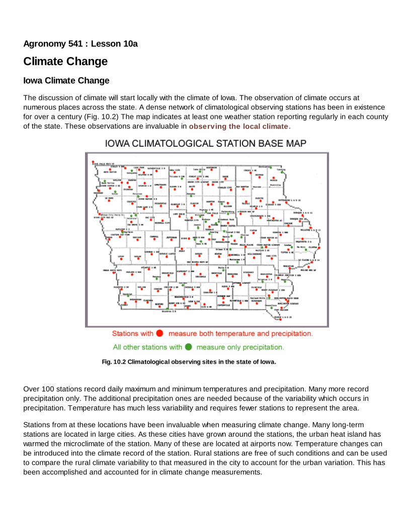
There is no question that the climate is changing. The world's temperature exhibits that changing climate. Butglobal changes are not the complete answer. Regional changes will exist and probably be the most concerning.Some areas would likely be winners and some losers. Included is an example for the Midwest combining thechanging global temperatures and heat stress for Iowa (Fig. 10.7). During the world's temperature increasefrom 1910 to 1940, stress on Iowa's crops varied extensively, resulting in very erratic yields. When the globalcooling trend began, the stress on the crop decreased for several years with very low stress and consistentyields.

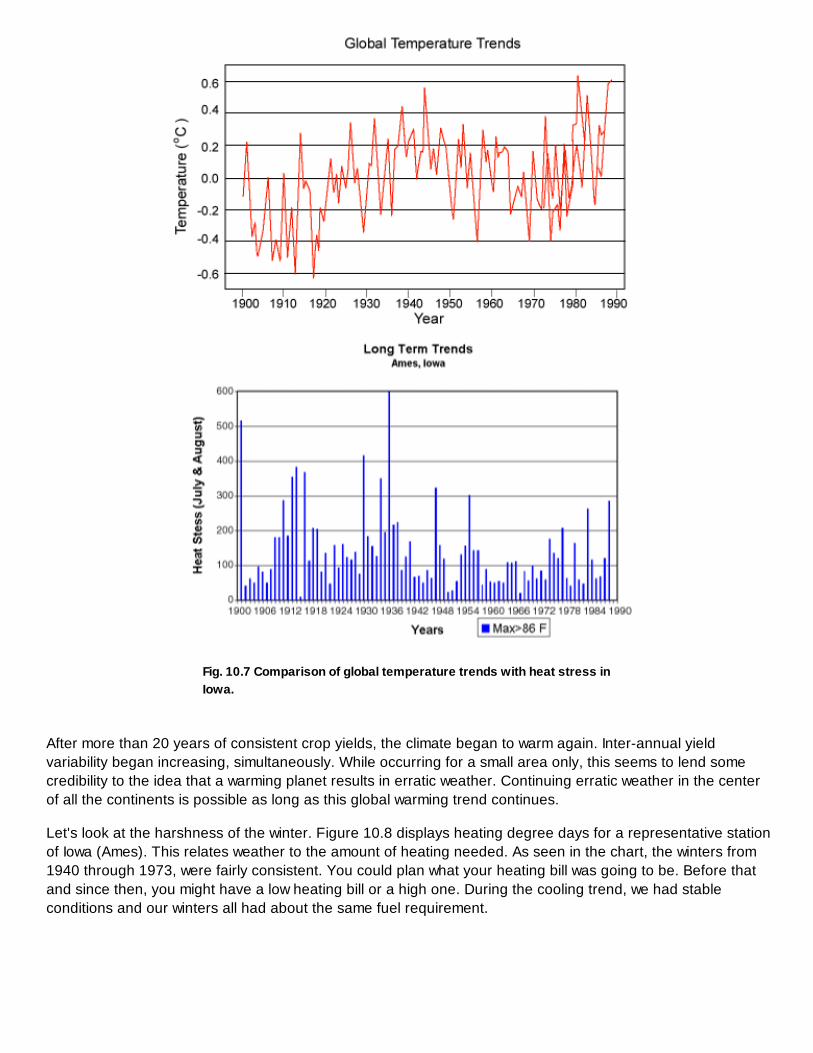
Fig. 10.7 Comparison of global temperature trends with heat stress in

Iowa.

After more than 20 years of consistent crop yields, the climate began to warm again. Inter-annual yieldvariability began increasing, simultaneously. While occurring for a small area only, this seems to lend somecredibility to the idea that a warming planet results in erratic weather. Continuing erratic weather in the centerof all the continents is possible as long as this global warming trend continues.

Let's look at the harshness of the winter. Figure 10.8 displays heating degree days for a representative stationof Iowa (Ames). This relates weather to the amount of heating needed. As seen in the chart, the winters from1940 through 1973, were fairly consistent. You could plan what your heating bill was going to be. Before thatand since then, you might have a low heating bill or a high one. During the cooling trend, we had stableconditions and our winters all had about the same fuel requirement.

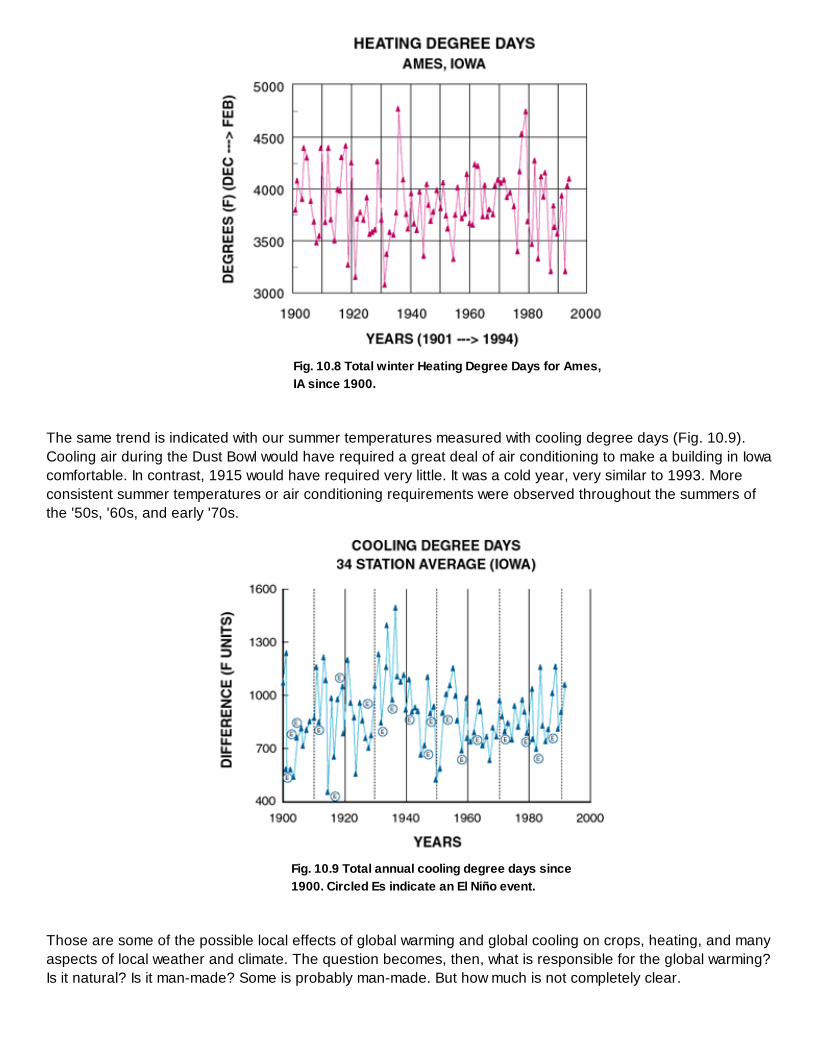
Fig. 10.8 Total winter Heating Degree Days for Ames,

IA since 1900.

The same trend is indicated with our summer temperatures measured with cooling degree days (Fig. 10.9).Cooling air during the Dust Bowl would have required a great deal of air conditioning to make a building in Iowacomfortable. In contrast, 1915 would have required very little. It was a cold year, very similar to 1993. Moreconsistent summer temperatures or air conditioning requirements were observed throughout the summers ofthe '50s, '60s, and early '70s.

Fig. 10.9 Total annual cooling degree days since

1900. Circled Es indicate an El Niño event.

Those are some of the possible local effects of global warming and global cooling on crops, heating, and manyaspects of local weather and climate. The question becomes, then, what is responsible for the global warming?Is it natural? Is it man-made? Some is probably man-made. But how much is not completely clear.


Climate Change

Causes of Temperature Change

There must be some forcing mechanism causing temperatures to change. To understand the possiblechanges, you have to understand what comes from the sun. The spectrum of sunlight was discussed in Lesson3b. How that radiation is affected in the atmosphere has a great deal to do with how the temperature willchange. The top line (Fig. 10.10) is the amount of radiation emitted by the sun reaching the top of theatmosphere. After entering the atmosphere, several wavelengths are affected by substances in theatmosphere. The lower line that has all of the squiggles up and down is the solar energy, which reaches thesurface of the earth.

Fig. 10.10 Spectral distribution of solar radiation, extraterrestrial and at sea

level, for a clear day. Each curve represents energy incident on a horizontal

surface (adapted from Gates, 1965).

Radiation is being absorbed at infrared wavelengths, primarily by water vapor. Water in the atmosphere andother greenhouse gases absorb part of the shorter wavelengths in sunlight and much of the longerwavelengths. They are even more important and effective in absorbing radiation beyond the sunlight into thethermal radiation bands. Here are some of the so-called greenhouse gases and what they absorb.

Fig. 10.11 Absorption spectra for various atmospheric gases

(Fleagle and Businger, 1963).

Study Question 10.4

Where does the atmosphere absorb the least amount of energy?

From 0.1 - 0.3 micrometersFrom 0.3 - 1 micrometersFrom 1 - 3 micrometersFrom 3 - 10 micrometersFrom 10 - 20 micrometers

Check Answer

Study Question 10.5

What band is that in?

UVVisibleIR

Check Answer

Study Question 10.6

Where does the atmosphere absorb the most?

From 0.1 - 0.3 micrometersFrom 0.3 - 1 micrometersFrom 1 - 3 micrometersFrom 3 - 10 micrometers

Check Answer

Study Question 10.7

What gas absorbs the most in this band?

MethaneNitrous OxideOxygen and OzoneCarbon DioxideWater Vapor

Check Answer

The wavelength of greatest concern is at 10 µ. Remember, most of the heat escaping from the earth is radiatedat 10 µ. Most of the radiation from 3 µ to 20 or 30 µ is absorbed and re-emitted. Water is the greatest absorberhere. Another one that influences at greater than 12 µ and around 4 µ is CO2. Oxygen and ozone have a fairly

narrow band between 9 and 10 µ. At longer wavelengths nitrous oxide and methane also made a radiationinfluence in their respective bands.

Water is the most important of the greenhouse gases. Huge amounts of water cover the planet. Water vapor isnecessary in the atmosphere to provide rain for life on the planet. In addition to its value for life it is animportant greenhouse gas. The temperature of the earth determines how much water there is in ouratmosphere.

Carbon dioxide is the most commonly discussed of the greenhouse gases. This has occurred primarily becauseof the huge amounts of carbon dioxide humans are moving from the earth to the atmosphere in the burning offossil fuels. For reference with other greenhouse gases, carbon dioxide is given an effectiveness of 1 in itsability to absorb and re-emit longwave energy. Every molecule of carbon dioxide in the atmosphere will have aneffect that we call 1 on the greenhouse of the earth. Other molecules are given a comparative effectiveness tocarbon dioxide.

Methane, which has been attributed to ruminant cattle and termites, has an effectiveness of 30 times the effectof carbon dioxide. Nitrous oxide, a bi-product of nitrogen emissions in the atmosphere, is 200 times as effectiveas carbon dioxide. Chloro-fluorocarbons (CFCs) are used as refrigerants in air conditioners and other useshave 14,000 times the effectiveness of carbon dioxide as a greenhouse gas. This creates a great concernabout the chlorofluorocarbons. It used to cost $2 to $5 to replace the freon in your automobile's air conditionerwhen it all leaked out. Now it costs you $35 or $40 because they're using a type of refrigerant which isn't agreenhouse and ozone-destroying gas. Because they destroy the ozone, CFCs have been banned, mandatinguse of another refrigerant.


Climate Change

CO2 Increase

The amount of carbon dioxide in the atmosphere is increasing. There is no question about that. Here are thecarbon dioxide measurements made at Mauna Loa, an observatory in Hawaii, since 1958 when the carbondioxide concentration in the atmosphere was 315 ppm, up to the present time at about 355 ppm. Figure 10.12has an annual cycle caused by heavy winter use of fossil fuels, followed by summer depletion as plants beginfixing the carbon dioxide. The overall trend is a significant increase in carbon dioxide levels. The total amountwill probably double before any controls can be enacted.

Fig. 10.12 CO2 observations at Maura Loa, Hawaii.

emit it toward the surface of the earth. The 315 ppm of carbon dioxide makes the surface of the earth about15° F (8° C) warmer than it would be without the carbon dioxide in the atmosphere. The theory was put forththat if CO2 makes the world 15° F warmer containing 300 ppm of carbon dioxide, doubling the carbon dioxide

would double the heating. Another 15° F would melt all the ice on the Poles and the Greenland ice cap, raisethe ocean 15-17 feet, and flood heavily populated coastal areas such as Washington D.C. and Florida. Thesewould be dire consequences. But the theory is mostly science fiction.

It turns out that carbon dioxide is absorbing about 80% of what carbon dioxide can absorb. (Refer back to Fig.10.11). Notice that most of the bands where CO2 is absorbing (the peaks near 1), it is absorbing almost as

much radiation in that band as possible. Doubling it, tripling it, quadrupling it, can only add about another 20%to the effect. Its primary effect was 15°F. Maybe another 3° F forcing from CO2 is possible with additional

continued accumulation. Accordingly, some people have doubted whether carbon dioxide is the problem.Maybe the other greenhouse gases are the problem.

Discounting carbon dioxide's importance is not appropriate, either. The CO2 increase has been dramatic. The

studies have estimated the carbon dioxide back to 1750 (Fig. 10.13). These measurements are made from icecores having little bubbles in them. Analyzing the air in the bubbles of ice indicates the atmosphericcomposition frozen into the ice. The ice cores provide a very consistent picture of the carbon dioxideconcentrations back to the 1700s. The carbon dioxide in the world's atmosphere then was about 280 ppm. Ithas climbed uniformly, accelerating during recent years, which were recorded by measurements since 1957.

Fig. 10.13 Pre-industrial CO2 concentrations obtained from published

observations of air trapped in ice cores. (From Lashof and Tirpak, 1989)

These are some of the issues with carbon dioxide in the atmosphere. Their influence on global climate changeis not known. The carbon dioxide amount has changed, but has it changed the temperature? Has it changedthe rainfall distribution? Has it changed the cloudiness? These are unknown factors. The potential for climatechange is a contentious and political issue because of the societal and economic factors involved.Unfortunately, the possible problems caused by greenhouse forced climate change may be ignored because ofthe political nature of the problem and our dependence on fossil fuels. So long as fossil fuel consumptionexceeds the Earth's processes of creating fossilized carbon, the atmospheric CO2 will continue to increase.


Climate Change

Sunspots

Some scientists think that the greater factor influencing global climate change is not the carbon dioxide at all,but the sunspots (Fig. 10.14).

Fig. 10.14. Dark spots are cool areas of the sun called sunspots.

Sunspots are an important aspect of our world and solar system. The ink blot (Fig. 10.15) is a drawing ofsunspots, the oldest sunspot picture available. A little line around the outside was drawn with a compass,indicating the outline of the sun. Spots were shaded in according to a solar image printed in a paper. This istoward the end of a sunspot cycle, because there are some big ones near the equator and some new sunspotsare forming near the Poles of the solar disc. This figure was drawn by Galileo, 3 May 1612. These are thebeginning of serious study of sunspots.

Fig. 10.15 Sunspots drawn by Galileo.

There were observations of sunspots known before 1600. Observations had been made in China and someother places. But before 1600 the records of sunspots weren't really good. They just knew that they existed.There were quite a few records in China near 1200. These records have been updated and the data utilized.But the observations are not consistent, because people made their observations of sunspots by lookingdirectly at the sun and writing down what they saw. The next time they wanted an observation, they had to get anew observer because the previous one was blinded.

A good record of sunspots does exist since 1612. Figure 10.16 is a record of sunspots over the last 240 years.Looking at one of these cycles, there is a period of time when there are very few or none. There are periods ofnumerous sunspots. Typically, a cycle takes 11 years from almost no sunspots, to the maximum, and back toalmost none. Forty-year periods occur where there are few sunspots, compared to the next 40- or 50-yearperiod. There are periods of time that sunspots are fairly rare, and periods of time when they are much morecommon. A 400-year record provides a good knowledge of these sunspot cycles.

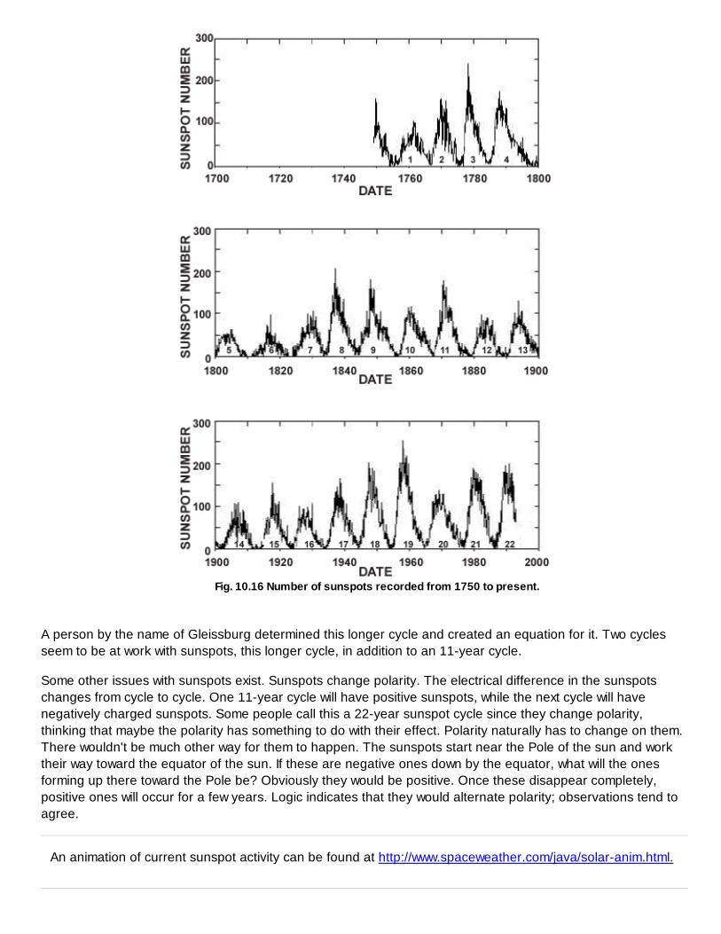
Fig. 10.16 Number of sunspots recorded from 1750 to present.

A person by the name of Gleissburg determined this longer cycle and created an equation for it. Two cyclesseem to be at work with sunspots, this longer cycle, in addition to an 11-year cycle.

Some other issues with sunspots exist. Sunspots change polarity. The electrical difference in the sunspotschanges from cycle to cycle. One 11-year cycle will have positive sunspots, while the next cycle will havenegatively charged sunspots. Some people call this a 22-year sunspot cycle since they change polarity,thinking that maybe the polarity has something to do with their effect. Polarity naturally has to change on them.There wouldn't be much other way for them to happen. The sunspots start near the Pole of the sun and worktheir way toward the equator of the sun. If these are negative ones down by the equator, what will the onesforming up there toward the Pole be? Obviously they would be positive. Once these disappear completely,positive ones will occur for a few years. Logic indicates that they would alternate polarity; observations tend toagree.

An animation of current sunspot activity can be found at http://www.spaceweather.com/java/solar-anim.html.

The ups and downs of the sunspots have a very strong influence on our radio communication. They have avery strong influence on the Northern Lights. The aurora and radio communication are the big things effects,probably the reason that money is spent analyzing, recording, and researching them.

People have tried to link sunspots with variations in weather. There is scant evidence of sunspot's effect onweather. There seems to be a correlation that about every 18-20 years the Midwest experiences a dry period.Some have attributed that to the 22-year sunspot cycle.

There has been at least one mechanism proposed by which the sunspots do have an influence on theatmospheric pressure quite high in the atmosphere. If they influence the atmospheric pressure, that couldmean they influence our weather at the ground since pressure is the crucial thing in determining if we're goingto have drought or floods. So there might be a mechanism that this 11-year up/down cycle has some influenceon our weather.

More likely influence may exist with this period of 40-50 years with few sunspots and 40-50 years with moresunspots in the cycle. A couple of interesting things have been found out about this. During the solar eclipsesin the early part of the century, the sun's diameter was measured. Measured during the next eclipse, it wasfound that the sun was larger. Further research indicated that, during periods of few sunspots, the sun issmaller than during sunspot maximums. Changes in the size of the sun could have a very definite influence onthe heating of the world.

A larger sun may produce more radiation. More radiation may heat up the earth. Is there anything to thattheory? In fact, there's a great deal to it. The blue part here at the bottom is the temperature of the earth. Seeit warming up from 1910 to 1940. It's all smoothed out, but that's the world's temperature, cooling from 1940 to1970 or 1972, and then warming up to the present time. And here's the length of the sunspot cycle. Theshorter the cycle, the warmer the Earth's temperature. Another comparison is with Figure 10.16. Note wheresunspot numbers are increasing, the planet warms, where they decrease, the planet cools. As the Gleissburgcycle starts going up, we have more total sunspots, and there we end up with a peak, and a couple of yearslater a peak on the world's temperature. The sunspots start back down around 1940. Down goes the world'stemperature. It tracks right along. Science magazine calls this a "dazzling correlation." This was taken fromScience, 1 November 1991, p. 254.

Global temperatures may somehow be related to the sunspot cycle. There is some reason to think that if thegreenhouse gases are going to cause global warming, their effect has not yet been seen. Many things can beexplained by changes in terrestrial and solar conditions.

Why is this important to us? First, if the erratic nature of the weather is going to continue as long as globalwarming continues, then we'll know something. If global warming is caused by humans increasing theirgreenhouse gas output, then global warming is going to continue until people change or change is enacted.

Early freezes could be more likely under global warming then under more stable global cooling conditions. Whywould we have an early freeze? More energy affecting the earth would produce more frontal activity. This couldallow a "bubble of air" (polar or Arctic air) to move southward. A bubble of cold Arctic air escaping from theArctic and coming down over the Midwest could result in an early or an unseasonably early fall freeze condition.One result of global warming could be a shorter growing season. It could be droughts, floods, or excessivecold. In fact, it would be most likely a combination of these things. If global warming does indeed cause ourweather to be more erratic, more tropical storms, droughts, and other negative aspects of weather will becomemore common.

If the global warming is being caused by the solar cycle, the Gleissburg cycle, then by 2012, temperatures willbegin to come back down. Weather will stabilize and agricultural output will again be consistent. In time all willbe apparent. However, it will be better if scientific analysis can explain global variation before a preventabletrend is out-of-control.

Agronomy 541 : Lesson 10b

Climate Cycles

Introduction


It is suggested that you watch Video 10B and complete the exercise in the video before continuing with thelesson.


Some of the cycles appearing in our weather and in our climate were discussed in lesson 7b. The mostobvious cycles are the daily cycle, caused by the earth's rotation, and the annual cycle, caused by therevolving of a tilted earth around the sun. The causes of these are very apparent. Other lengthier cycles canbe related to other orbital relationships of the earth. Lesson 10a presented possible cycles associated withsunspots. This part of the lesson discusses some other cycles in the atmosphere. Anyone can see that manycycles do exist. Some cycles are touted, but do not yet have an accepted cause and effect. Some reportedcycles have little validity.




Climate Cycles

Detection of Climate Change and Cycles

In the past million years or so some climatic cycles are very obvious (Fig. 10.17). The growth of glaciersperiodically is well accepted. What evidence exists to indicate cold periods? There are no measurements.Measurement records in the United States extend back 100-150 years. Locations in Europe have records for afew hundred years in a few cases. In comparison to millions years of climate history, the measured record is aninsignificant by comparison. While not having measured data, much can be inferred from other data sources.Cold periods are often implied by the materials that are in lake sediments or in ocean sediments. They areoften implied by ice build-up in glaciers, at least back for several thousands of years.

Fig. 10.17 Reconstructed global temperatures over the last 850,000

years.

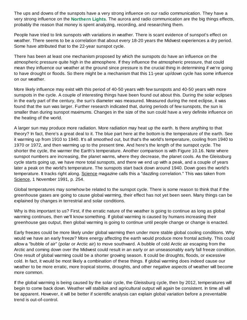
Data such as these are called proxy data, where climatic conditions can be inferred from secondary datasources. The measurement of sediment thickness and the biological content of the sediment give clues to whatthe climate of the drainage basin was like during the period. The most well defined proxy data are tree rings(Fig. 10.18). Trees are integrators of the climate they are exposed to. The width of tree rings is related to theclimate of a growing season. Wide rings are usually wet years with good growing conditions. Narrow rings aredry years or have poor growing conditions for some reason. Data from tree rings has been used to examine thedrought records of the western United States for the last several hundred years.

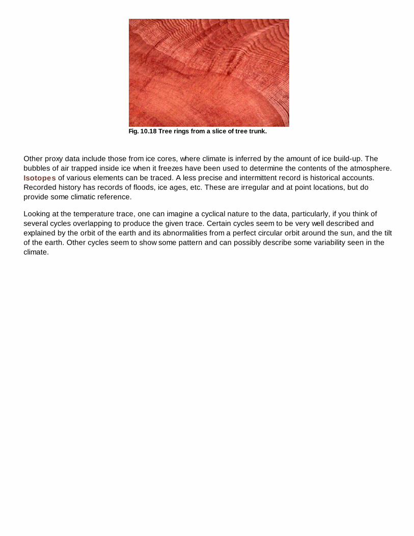
Fig. 10.18 Tree rings from a slice of tree trunk.

Other proxy data include those from ice cores, where climate is inferred by the amount of ice build-up. Thebubbles of air trapped inside ice when it freezes have been used to determine the contents of the atmosphere.Isotopes of various elements can be traced. A less precise and intermittent record is historical accounts.Recorded history has records of floods, ice ages, etc. These are irregular and at point locations, but doprovide some climatic reference.

Looking at the temperature trace, one can imagine a cyclical nature to the data, particularly, if you think ofseveral cycles overlapping to produce the given trace. Certain cycles seem to be very well described andexplained by the orbit of the earth and its abnormalities from a perfect circular orbit around the sun, and the tiltof the earth. Other cycles seem to show some pattern and can possibly describe some variability seen in theclimate.

Close Window

FYI : Isotopes

Isotopes are elements with different numbers of neutrons in their nucleus. For instance, there are three forms ofcarbon, carbon-12, -13, and -14. The latter two having 1 and 2 extra neutrons. These are radioactively unstable andwill decay over time to carbon-12. How much of these isotopes are in a sample indicates the age of that sample. Thisis a dating process called carbon dating.


Climate Cycles

18-20 Year Cycle

One of these shorter term cycles (called the 20-year cycle) is often cited by people who speculate on cropyields using cycles. Their reasoning was that yields were very bad in 1936, fairly low in 1955, and low in 1974.This was extrapolated to a 19 or 20-year cycle. Clearly, in their thinking, there was going to be another greatdrought, probably as bad as 1936, in 1993.

Some private climatologists and meteorologists were claiming this in advance of 1993. The supposed droughtwould be worse than the one in 1988. The resulting weather in 1993 was quite the opposite, nearly drowningthe Midwest. The next year, some private meteorologists claimed a miss in 1993, but said that the droughtwould certainly happen in 1994. In 1994, record yields were set. The claim was repeated in 1995 since theMidwest was "overdue." The year was not a wonderful growing year. Temperatures were wet in the spring , dryin the summer, and wet in the fall (Fig. 10.19). However, no widespread drought occurred.

Fig. 10.19 Palmer Drought Stress Index maps for 1995. Negative

numbers are increasing drought severity.

Since the predicted drought did not happen as forecast, some think that the likelihood of drought occurring isincreasing. But the drought has not occurred in the 19th, 20th or 21st year of the cycle. Is there validity to thiscycle? There is something to this 18 or 19 year cycle. Forecasting a great drought because of it is not possible,but some climatic relationships do exist.

The oldest building in St. Petersburg (Fig. 10.20), formerly Leningrad, was built by the River Neva, which, onoccasion, floods. They have marked the dates and height of the floods on the wall of the building for more than250 years (Fig. 10.21). Interestingly, the first flood occurred soon after they established the city of St.Petersburg. Nineteen years later they had another one. Eighteen years later they had another one. Twentyyears later they had another one. Adding 18.6 to the initial flood year produced a number within a year or ayear and a half of all of the floods up to the present time. The floods are on an 18-year cycle. Not all floods fitthe cycle but the pattern is apparent.

Fig. 10.20 Outside wall of Peter and Paul

fortress

Fig. 10.21 Inside marks of floods

The Museum of Texas History in San Antonio had a display of a little city located near the Rio Grande River.They claimed this city and the river had an 18-year flood cycle. They called it the "well-known" 18-year floodcycle of the Rio Grande.

The center of every continent seems to have an 18.6-year cycle of drought, floods, or some weatherphenomena. Whether it was the probability of having these droughts, or not, leaves us something to wonderabout. Now was 1936 the time to start looking at this, or was it 1934 that should have been "year 1" of the 18-year cycle? Or was it 1930 when the Dust Bowl started? There does seem to be a cycle of flooding or droughtthat goes on in the center of continents. The center of Africa, South America, North America, and Asia seem tohave an 18.6-year cycle. Antarctica is an unknown because of the scarcity of data over the continent.

What makes that 18-year cycle if it is real? Some people claim that sunspots control it. Sunspots cycle every20-22 years, fairly closely to the 18-year cycle. Sunspots could appear to influence the cycle, because over aperiod of time when the sunspot numbers would be down, the Midwest would be in or near a dry period (Figs.10.22 and 10.23).

Fig. 10.22 Sunspot number, polarity and associated climatic conditions

over the last 200 years.

Fig. 10.23 Sunspot number and polarity with associated climatic

conditions over the last 200 years.

Figures 10.22 and 10.23 compare "sun spot and lunar cycles". The line indicates sunspot cycles, whichalternate positive and negative. Notice a couple of things. The drought and extreme heat of 1934-36 occurredwhen the sunspot numbers were low between a negative and a positive cycle. Some drought occurred between1954 and 1956. Rainfall was reduced, but temperatures were cooler, making the droughts less severe. Thisalso occurred in the low point between the negative and the positive sunspot peak. In the early seventies,sunspot numbers were heading down but not at the bottom. The phase between the negative peak and thepositive peak was correct. Another cool drought occurred. The drought in 1988 was different. The droughtoccurred when conditions should have been wet, between the positive and negative phase. This does notinvalidate the cycle as cycles do not preclude a "good" year at a bad time nor a bad year during a "good"period.

Study Question 10.8

According to the chart, what should our conditions have been like in the late 1990s?

W t

WetDry

Check Answer

The correlation has occurred for only 3 cycles. This could be mere coincidence. A longer recurrence of thecycle needs to be observed to prove the correlation. Sunspots are recorded from 1600. Looking back, whenwere some of these other droughts? Droughts in the 1800s did not follow the same cycle. Several droughtsoccurred at the sunspot minimum, but between the positive and the negative phases. The great drought of1901 was between the positive and the negative phase, opposite to phase shift of this century. Therefore,sunspots cannot be shown to have anything to do with the cycle at a high confidence level.

A renowned independent climatologist has claimed the sunspot effect reversed in phase every hundred years.But no reason can be given why it should reverse every hundred years.

Figure 10.22 also mentions lunar cycles. The moon has a gravitational effect on the earth. Ocean tides dependon the position of the sun, the moon, and the earth, with relationship to each other. Tides do follow the lunarcycle exactly, except for some minor wind variations.

Isaac Newton solved this with the theory of gravity, relating the moon's effect on tides. The 18.6-year lunarcycle is noted in Figure 10.23. Notice the occurrence of dry spells and the lunar cycle. The sunspot cycle didn'tcorrelate well with droughts in the 1800s. But looking at the Moon's relationship of dry periods, the correlationis very good. The moon cycle, at least for 200 years, has been right in phase with recorded dry periods.

So there could be a tidal effect on the atmosphere, affecting the highs and lows of the oceans and the highsand lows of the atmosphere. It could have an effect on the precipitation pattern; research is ongoing at thepresent time. There may be something to a lunar cycle and the cycling that apparently affects the rainfall andagriculture in the Midwest. Also solar activity may be related to the pressure changes in the highest levels ofthe atmosphere.

One recently reported correlation was between the length of the sunspot cycle and the change in globaltemperature over the last century (Fig. 10.24). According to this study, there is then a relationship between thelength of the cycle and global temperatures. Whether they are correlated with each other and caused bysomething else is not known. While the correlation is very interesting, no physical reasoning is given, yet.

Fig. 10.24 Length of the sunspot cycle compared to global

temperatures over the last century.

S l i thi bl ith th t d l l ld lid t th b i it f l

Solving this problem with the sunspot and lunar cycle would validate more then even observing it for severalmore cycles. The lack of physical reason why this cycle would affect the weather is most problematic. Whetherthe cycle can be seen is arguable. But for general acceptance the underlying physical effects must beexplained.


Climate Cycles

Other Orbital Effects

Some of the variability in climate can be explained by cycles in the Earth's orbits. These were discussed inLesson 7b. The earth is not in a circular orbit around the sun. It is in an almost flattened orbit approaching anellipse. At the present time, in the winter the earth is closer to the sun than in the summer. In a few thousandyears, this will not be so. The earth will be closer to the sun in the summer in the Northern Hemisphere than inthe winter. It will make our summers a little bit warmer. At the same time a diminished tilt may reduce summerheating.

As early as 1600 Kepler determined that the earth's orbit was elliptical. There was, also, going to be a 22,000year cycle of the earth being closer to the sun in the winter or closer in the summer, associated with the wobbleof the earth.

Over the last 800,000 years, relatively recent time geologically, there have been several swings in globaltemperatures from ice ages to warm periods. The history of the temperature of the earth as recorded in the iceis shown in Fig. 10.25.

Fig. 10.25 Reconstructed global temperatures over the last 850,000

years.

ver the last 800,000 years, rather recent times geologically, North America has experienced an ice age. Therewas a warm interglacial time about 120,000 years ago. Then the glaciers of our most recent glaciation formedand covered most of North America. About 10,000 years ago they retreated into Canada. During the meltingthey formed many of our geologic features such as the basin of the Columbia River and many lakes.

Currently, we are in a warm interglacial period of an ice age. Technically, the earth is still in the ice age. Ice stillexists on the Poles, but it is interglacial. We do not know if we are going to heat now in the next few thousandyears and come out of the ice age. During most of the history of the world, temperatures have been warmerthan the present temperature (indicated by the top line in Fig. 10.25). During the last million years or so theearth has been running on the cold side of this line. In other words, ice ages have not been as predominant as

during the past 800,000 years.

What causes the ice ages? The orbit of the earth causes ice ages. At least that was the theory that wasbrought forth some time back by a person who worked in Russia named Milankovitch.

It was a person by the name of Kroll, who in 1875, found that the ice ages corresponded almost exactly withorbital irregularities and the angle of the earth. Milankovitch in 1890 added a third cycle to this, the precessionof the earth. Comparing the three cycles and the ice volume began to match each other very well. Figure 10.26shows the three cycles put together mathematically. Adding the actual ice observations produces the secondpart. Adding the carbon dioxide change on the earth to the pictures of the ice observations and the picture ofthe orbits produces an almost identical figure.

Fig. 10.26 100,000 year cycle os depicted in the ice volume (bottom) over the

last 1,000,000 years. Note that ice periods are associated with decreased

solar insolation.

Scientists are fairly well convinced at this period of time that the big climate changes on the earth, the ice agesand the interglacial periods, have depended upon the analysis of Milankovitch orbital considerations. Aconnection of the Milankovitch to changing carbon dioxide is proposed (Raymo, 1998). by M. E. Raymo in"Science" Vol.281, 4 Sept. 1998, under the title "Glacial Puzzles".


Climate Cycles

Cycles

Now are there other cycles? As mentioned in lesson 1, the moon has an 18.6-year cycle. The sunspots have a22-year cycle. Are there other cycles that influence our weather?

Cycles that are absolute are the 24-hour one and a 1-year cycle. As the cycles get longer, they are less sure.A 1-year cycle is a pretty sure cycle. We can plan on most days in January being colder than most days in July.There might be one day in January warmer than some one day in July on some rare occasion, but for the mostpart, the cycle is a pretty sure thing.

The 11,000 year cycle that had to do with the tilt of the earth and the 22,000 year and 100,000 year cycles thathad to do with orbital considerations of the earth seem to be real cycles. Is there anything in between that isreal? Does the 18.6-year cycle that influences the tides of the ocean so dramatically affect our climate? Theeffect of the moon on the tides is very well known. Every 18.6 years we have the high tides and great floodproblems from high tides. These are very well understood as an 18.6-year cycle. Does it influence theweather? It is not particularly clear if it does or does not. Looking at tree rings and other data, a cycle that ismaybe 18.6 years or maybe 20 years seems apparent.

There also appears to be a 60-year cycle that influences our weather in the Midwest. The Midwest had somepretty rough weather in the 1930s with the Dust Bowl, in the 1870s and the 1810s. The 1990s were a time ofconcern because there seems to be a 60-year cycle of irregularity in the weather. The 60-year cycle isassociated with sunspots. In addition to the 22-year and 11-year sunspot cycles, there may be one between 60and 90 years long called the Gleissburg Cycle.

There is the very definite 176-year cycle for the retrograde motion of the sun. It is most noticeable to peoplewho carefully chart the sun with instruments and to astronomers. It is probably not noticeable to the rest of us,unless the weather really is bad during that time. Some articles have claimed that a great drought is going tooccur because of the retrograde movement, but nobody can figure out what the connection to weather is.Going back to the previous one 176 years ago, bad weather did occur. We have found no reason to think thatthis is significant to our weather.

None of these have much credibility in influencing the world's weather. There remains much uncertaintyregarding cycles longer than one year and shorter than 5000 years.


Climate Cycles

Cycle Effect on Temperature

One very definite temperature cycle or temperature effect that we have seen is called the little ice age whichoccurred about 400 years ago in 1600 A.D. The Earth was fairly warm at 800 years ago (Fig. 10.27). At 700years ago, it cooled off appreciably. Slight warming occurred in the middle 1500s while cooling back off 280years ago. This cool period from 1600 to 1700 was well observed. Lots of scientists were watching it. The timewas one of great scientific discovery. Scientists and most everyone associated with agriculture in Europenoticed that the earth was cooling off. Farmers' crops did not mature; there was a lot of irregularity of theweather. It was not very different from year to year or month to month, but it was getting harder to grow crops inFrance and in England. We went through a minimum of sunspots and received less energy from the sun.

Fig. 10.27 Temperature variation over Europe in the last 1000

years.

Looking at the geometry of the Earth's orbit we can say there was a geometric effect of the Earth's orbit thatmay have had something to do with the cooling during this time. Perhaps the sunspots had an effect. Sunspotswere minimal during the little ice age (1620-1710). When the sunspots returned, the earth started warming,continuing until 1940 when the earth started to cool off again (Fig. 10.28). The earth began an appreciablecooling from 1940 until 1972. In 1972 the earth began another appreciable warming.

Fig. 10.28 Global average

temperature trend (1880-1990).

In the past 200 years the planet was cooling, the planet was warming, the planet was cooling, and the planet isnow again warming. Is that a cycle or is it a coincidence? This is not entirely clear. Nevertheless it is somethingthat is going on and is influencing our weather. We do not really know if it is a man-made effect that we areseeing right now with this warming, or if it is just a part of this natural cycling that has gone on occasionally withups and downs in the weather.


Climate Cycles

Using Cycles to Forecast

One forecast based on cycles was originally discovered back in the year 1885. Somebody plotted grain pricesand published it in 1937 in Dunn's Review, October issue, 1937, page 42. It showed ups and downs from 1800to 1885 in the grain markets. This appeared as a definite "M" pattern. This "M" pattern was produced by poorgrain prices because of plentiful grain. Then a couple of droughty years would occur during a 6-year period.The droughts drove prices up. During the next 12 years, there would maybe be one drought allowing prices tobounce around a little bit. Then grain would be very plentiful. And the cycle would begin again. The basicmessage was that during a 6-year period, two droughts would occur. Then, a 12-year period would have one.This basic pattern described crop prices from 1800 to 1885. Assuming the pattern was regular, the figure wasdrawn out to the year 2000 (Figure 10.29). The cycle pattern was identified by 1880 by Samuel Benner (1891).

Fig. 10.29 Periodic return of drought years and consequent

economic hardships.

Click on the image for an enlarged view (from Dunn's

Review, 1937).

According to the figure, sometime between 1932 and 1938, there would be some bad droughts. Basically, theauthor forecasted the Dust Bowl. The cycle captured the drought of 1901 and others. Going out to the year2000 with this same pattern, the figure shows that, after 1986 through 1992, the drought risk has passed. Thegreat drought risk had 1988 right in the middle of it.

If this analysis is correct it would say that we are beyond the high risk of drought, until the year 2004. The onedrought will be a minor one. The awful one was caught in the 1988 period. While this has not been proven, theforecast record is good for over 200 years.

Assignment 10.1

Click here for Assignment 10.1

Lesson 10 Reflection

Why reflect?

Submit your answers to the following questions in the Student Notebook System.

1. In your own words, write a short summary (< 150 words) for this lesson.2. What is the most valuable concept that you learned from the lesson? Why is this concept valuable to

you?3. What concepts in the lesson are still unclear/the least clear to you?4. What learning strategies did you use in this lesson?


Climate Cycles

References

Benner, Samuel. 1891. Benner's Prophecies. Robert Clarke and CO. Cincinnati. pp 196

Bryson, R.A and T.J. Murray 1977: Climates of Hunger : mankind and the world's changing weather. Madison,WI : University of Wisconsin Press, 171p.

Karl, T. R., R. W. Knight, D. R. Easterling, and R. G. Quayle, 1996: Indices of climate change for the UnitedStates. Bull. Amer. Meteor. Soc., 77, 279-292.

Mathews, S.W., 1976: What's Happening to Our Climate? National Geographic, 149: 576-615.


Climate Change

Introduction


It is suggested that you watch Video 10A and complete the exercise in the video before continuing with thelesson.


Climate is changing. Climate has always changed. Climate will always change. The issue is how much it willchange, how fast will it change and why does it change? The contribution of human activities to climate changeis much debated and still being understood.

Excessive cooling or warming could lead to disastrous effects on society. Where the climate is going is a hugeconcern. Sunspots have been considered to be important as long as people have known about them. Theyhave been observed for several centuries. More than for their effect on communications, sunspots may haveother effects on the earth and its climate.

The concept of a "greenhouse effect" was proposed in the 1800s. Is the greenhouse effect responsible forincreasingly erratic weather and is it associated with observed global temperature changes of the next onehundred years? There can be no doubt that climate is changing and that the change impacts every aspect ofsociety.



Reading Assignments:

pg. 435-464—Aguado and Burt

Documents

Climate Change - Iowa State Universityagron-€¦ · The climate is changing around us in changing. Where it is going and why are open to great debate. How much is natural and how