THE UNIVERSITY OF TEXAS ATAUSTIN

Climate Change Impacts on the Water Resources An overview of global Impacts and techniques to assess at local scale

Literature Review

Eusebio Ingol - Blanco November 18, 2008

GEO 387H – Physical Climatology Dr. Zong-Liang Yang

Fall 2008

1

Abstract

This document presents an overview over global impacts on hydrology and water resources as

consequence of climate changes. Likewise, in order to evaluate these impacts at local scale, main

downscaling techniques and some applications are reviewed. At the global scale, precipitation

will increase in some regions such as part of tropics and high latitudes and decreases in lower

and mid latitudes. Runoff depends of the changes in precipitation; in this sense, it is noted a

reduction in central American and Europe. Risks of droughts are projected for sub tropical, low

and mid latitudes and floods for tropical and highs latitudes. Changes in groundwater recharge,

soils moisture and evaporation are also reviewed. Likewise, some results from GCMs, climate

change will affect directly on the water resources systems, indicating that in next 50 years will

increase the water stress on land areas. On the other hand, statistical and dynamical methods are

discussed. Statistical downscaling is classified in stochastic weather generators, regression

models, and weather pattern approach. Dynamic downscaling develops and uses a regional

climate model (RCM) with the course GCM data used as boundary conditions. Both techniques

show great skill to perform the downscaling data. Finally, this paper presents a general

procedure to incorporate the climate change impacts on hydrological and water resources

models.

1. Introduction

Climate variability has relevant importance on the hydrology and water resources availability in

the world. Changes in temperature and precipitation patterns as consequence of the increase in

concentrations of greenhouse gases may affect the hydrology process, availability of water

resources, and water use for agriculture, population, mining industry, aquatic life in rivers and

lakes, and hydropower. Climate changes will accelerate the global hydrological cycle, with

increase in the surface temperature, changes in precipitation patterns, and evapotranspiration

rate. The spatial change in amount, intensity and frequency of the precipitation will affect the

magnitude and frequency of stream flows; consequently, it increases the intensity of floods and

2

droughts, with substantial impacts on the water resources at local and regional levels. Global

climate simulations indicate that precipitation will decrease in lower and mid latitudes and

increase in high latitudes (IPCC, 2008). Results show that rainfall will decrease in Caribbean

regions, sub tropical western coasts, part of North American (Mexico), and over the

Mediterranean. Evaporation, soils moisture content, groundwater recharge will also affected by

climate changes. Drought conditions are projected in summer for sub tropics, low and mid

latitudes. Some results show that for warmer climate the drought increases from 1% to 30 % in

2100. On the other hand, global impacts on the water resources show that freshwater for

different uses will be affected.

According to IPCC, a notable reduction of the water resources service is projected where the

runoff decrease, and also the projection of water stress for 2050 s indicates a increase in range of

62-76 % of the global land areas. On the other hand, to assess these impacts at the local scales,

downscaling techniques need be applied. In that context, Statistical and dynamical methods are

used in hydrologic and water resources studies. Statistical downscaling allows relates the large

scale climate from GCMs with the historical (local) scale variables. This method is classified in

regression models, stochastic weather generation, and weather pattern approach (Wilby, 1997).

Dynamic method uses complex algorithms to describe the atmospheric process and whose goal is

to extract the local weather data from large scale GCM. Based on several studies, both

methodologies have performed efficiently; however, the dynamic downscaling is a method more

sophisticated that requires of large amount of computational resources.

3

2. Climate Impacts on the Hydrology and Water Resources

2.1 Impacts on the hydrology cycle

The main components of hydrology cycle are the precipitation, evaporation, runoff, groundwater,

and soil moisture, and it is liked with changes in atmospheric temperature and radiation balance.

According to IPCC (2008), precipitation pattern over 20th century has shown important spatial

variability; which has decreased from 10o S to 30 o N latitude and increased in high northern

latitudes since 1970. In addition to this, precipitation increased around 2% between 0 oS to 55 oS

and from 7 to 12 % from areas located between 30 oN to 85 oN (IPCC, 2001).

On the other hand, for the 21st century, simulations with climate models indicate a increase in the

globally evaporation, water vapor, and precipitation, indicating that precipitation will decrease in

the lower and mid latitudes regions while it increases in high latitudes and part of tropics (IPCC,

2008). Figure 1 shows the mean change in precipitation of fifteen climate models for the scenario

A1B (from December to February: DJF and from June to August: JJA). It is noted that

precipitation decreases over several sub tropical areas and mid latitudes (for summer) while for

tropical oceans and in some monsoon regimens such as South Asian monsoon summer the

precipitation increases. The global annual mean precipitation change (in percentage) for the

period 2080 – 2099, for the SRES A1B scenario, is presented in figure 2 (from IPCC, 2008).

Important decrease of up 20% will occur on the Caribbean regions, sub tropical western coasts in

most countries, and over the Mediterranean. For instance, all Central American, Mexico and

south USA will be affected by a significant reduction in precipitation. Increase in annual

precipitation in more than 20 % will occur high latitudes such as in Northern part of central Asia,

Eastern Africa, and the Equatorial Pacific Ocean. Changes in soil moisture depend basically of

the precipitation and evaporation which may be affected by changes in the land use; therefore its

4

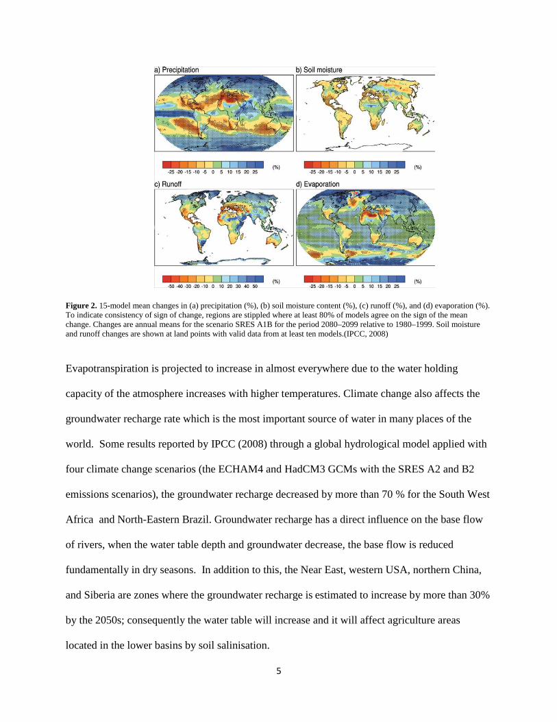
spatial variation is a little different from the changes in precipitation. Projections indicate that the

annual mean soil moisture content increases up around 15 % in some regions where the

precipitation is increased, East Africa, and central Asia (figure 2b) while it decreases in sub

tropical and Mediterranean zone. Changes in stream flows in rivers depend fundamentally of the

change in the volume and time precipitation, and some cases of the snow melting. Figure 2c

shows the change in global runoff under A1B scenario. Runoff is clearly reduced in Central

American, part of Mexico, and Europe; however it is increased in high latitude rivers.

Additionally, in figure 2d is shown the global evaporation. It is noted that annual evaporation

increases over most oceans (surface temperature increase). At the global scale, mean evaporation

changes balance global precipitation but it is different at local scale due to changes at the

atmospheric transport of water vapor (IPCC, 2001).

Figure 1. “15-model mean changes in precipitation (unit: mm/day) for DJF (left) and JJA (right). Changes are given for the SRES A1B scenario, for the period 2080–2099 relative to 1980–1999. Stippling denotes areas where the magnitude of the multi-model ensemble mean exceeds the inter-model standard deviation”. (IPCC, 2008). DJF (December, January, and February), and JJA (June, July, and August).

5

Figure 2. 15-model mean changes in (a) precipitation (%), (b) soil moisture content (%), (c) runoff (%), and (d) evaporation (%). To indicate consistency of sign of change, regions are stippled where at least 80% of models agree on the sign of the mean change. Changes are annual means for the scenario SRES A1B for the period 2080–2099 relative to 1980–1999. Soil moisture and runoff changes are shown at land points with valid data from at least ten models.(IPCC, 2008)

Evapotranspiration is projected to increase in almost everywhere due to the water holding

capacity of the atmosphere increases with higher temperatures. Climate change also affects the

groundwater recharge rate which is the most important source of water in many places of the

world. Some results reported by IPCC (2008) through a global hydrological model applied with

four climate change scenarios (the ECHAM4 and HadCM3 GCMs with the SRES A2 and B2

emissions scenarios), the groundwater recharge decreased by more than 70 % for the South West

Africa and North-Eastern Brazil. Groundwater recharge has a direct influence on the base flow

of rivers, when the water table depth and groundwater decrease, the base flow is reduced

fundamentally in dry seasons. In addition to this, the Near East, western USA, northern China,

and Siberia are zones where the groundwater recharge is estimated to increase by more than 30%

by the 2050s; consequently the water table will increase and it will affect agriculture areas

located in the lower basins by soil salinisation.

6

In some regions is projected to increase the risks of droughts and flooding due to the increase of

the intensity and variability of the precipitation for the 21st century. Dry periods are projected for

mid continental zones in summer (sub tropics, low and mid latitudes), with marked risk of

droughts in these regions. Likewise, extreme rainfall is projected to increase in tropical and high

latitudes regions that experiment increases of the mean precipitation. For instance, results from

15 AOGCM runs for the future warmer climate show that the extreme drought increases from

1% at the current day land area to 30 % in 2100 for the A2 emission scenario (IPCC, 2008).

2.2 Impacts on the Water Resources Management

As it was discussed in the section above about the potential effect of climate change on the

precipitation, stream flows, groundwater recharge components which would affect directly over

the water resources availability in regions above all in those under climate stresses. This situation

even more complicated if the characteristics and policies of water resources management

systems are not adequate to mitigate these changes. Water for agriculture, population,

hydropower, water pollution control, mining industry, etc, are depending on the hydrological

cycle. In this sense, climate change affects the management and operation of existing water

infrastructure such reservoirs, structural flood defense, channels, dams, irrigation systems, and

hydropower plants. Irrigation methods and water management practices also will be affected.

Likewise, in many places in the world, the main water resources for agriculture and urban uses

come from base flows in rivers and groundwater (for dry periods) which will be affected due to

the changes in the recharge groundwater (effect on aquifers in long term). Changes in runoff and

water availability influence over it. In addition to this, increase in melting snow in some regions

like the Andes in South America contribute in the short time to increase the runoff and in the

long term to reduce the snow area; consequently a reduction of water availability understanding

7

that some places, it is the main source of water use. On the other hand, raising sea level increases

the possibility of sea intrusion into coast aquifers affecting the groundwater use due to the high

salinity concentrations.

In global terms, water demand will grow in the next decades due to the population growth and

regionally, substantial changes in irrigation water demand are expected as results of climate

change (IPCC, 2008). In general, negative effects of climate changes on water resources systems

would complicate the impacts on the changing economic activity, water quality, increase

population, land use change and urbanization. According to IPCC (2008), in the 2050s “the area

of the land subject to increasing water stress due to climate change is projected to be more than

double than with decreasing stress”. A clear reduction of the water resources services is shown

in zones where the runoff is projected to decrease and the others where the rainfall increases,

increased total water supply are projected. However, probably this benefit can be reduced by the

negative effects of higher variability of the precipitation and seasonal runoff in water supply,

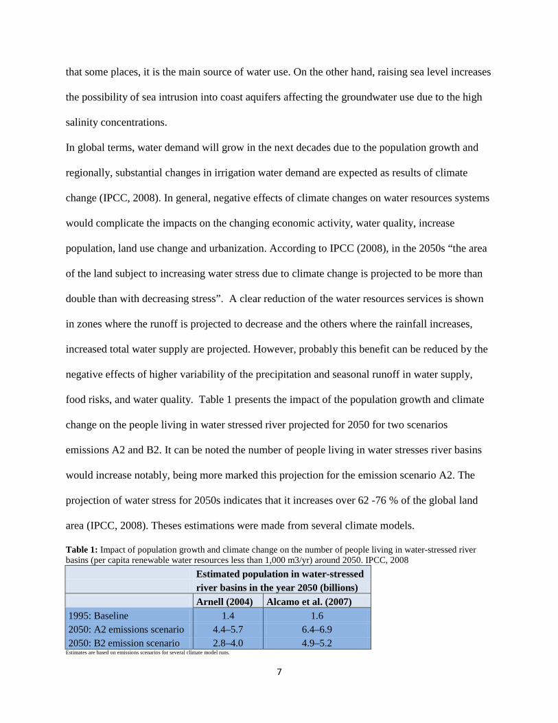
food risks, and water quality. Table 1 presents the impact of the population growth and climate

change on the people living in water stressed river projected for 2050 for two scenarios

emissions A2 and B2. It can be noted the number of people living in water stresses river basins

would increase notably, being more marked this projection for the emission scenario A2. The

projection of water stress for 2050s indicates that it increases over 62 -76 % of the global land

area (IPCC, 2008). Theses estimations were made from several climate models.

Table 1: Impact of population growth and climate change on the number of people living in water-stressed river basins (per capita renewable water resources less than 1,000 m3/yr) around 2050. IPCC, 2008 Estimated population in water-stressed river basins in the year 2050 (billions) Arnell (2004) Alcamo et al. (2007) 1995: Baseline 1.4 1.6 2050: A2 emissions scenario 4.4–5.7 6.4–6.9 2050: B2 emission scenario 2.8–4.0 4.9–5.2

Estimates are based on emissions scenarios for several climate model runs.

8

Figure 3 shows the future climate change impacts for freshwater elaborated by IPCC on the base

of different studies about climate change impacts on water resources in the world. It should be

noted that stream flows decrease and the demand will not be satisfied after 2020 in Central

America and Mexico; the results indicates a reduction of the stream flows around 25 % for these

regions. North and south Africa, Europe show the same trend.

Figure 3. Future climate change impacts on the freshwater which threaten the sustainable development of the affected regions. 1: Bobba et al. (2000), 2: Barnett et al. (2004), 3: Döll and Flörke (2005), 4: Mirza et al. (2003), 5: Lehner et al. (2005), 6: Kistemann et al. (2002), 7: Porter and Semenov (2005). Background map, see Figure 2.10: Ensemble mean change in annual runoff (%) between present (1980–1999) and 2090–2099 for the SRES A1B emissions scenario (based on Milly et al., 2005). Areas with blue (red) colors indicate the increase (decrease) of annual runoff. (IPCC, 2008) Another interesting aspect is related with glaciers and snow cover which are projected to

decrease due to increase of the surface temperature. Consequently reducing the water availability

during dry periods in regions contributed by the melting snow water from mountain ranges

where currently one-sixth of the world’s population is located. Water quality will be another

problem in the future. Higher water temperatures and extreme events of the precipitation are

9

projected to affect the water quality and increase many form of water pollution. Oxygen

concentrations would be reduced due to the increase of the water temperature (IPCC, 2008).

As it is noted there will have multiples climate impacts in the future on the hydrology and water

resources. Here only the most important issues have been mentioned.

Finally, to face these impacts in the future, period of transition and adaptation must be designed

in order to guarantee the water supply fundamentally for drought periods. Strategies need be

developed and applied according to the reality of each water resources system. These strategies

should be focused to improve the water use efficiency through the modernization of hydraulic

infrastructures, development of water markets, water conservation plans, change the crop

patterns with less water consumption (reduce the demand), change irrigation methods, build

structural flood defenses, improvement of the water management policies, in some case increase

the storage capacity of the reservoirs, etc. Additionally, many places with stresses water,

generally in poor countries; there is a deficit of storage structures such as reservoirs and dams

that does difficult to face the climate change impacts at current conditions. In this sense, it is

necessary to build storage systems that allow mitigating these effects within of framework of

integrated water resources management and environmental protection.

As it was mentioned, the changes described above are at global scale. At the local scale, several

studies about changes in precipitation, runoff, and soil moisture using different emission

scenarios have been carried in the many basins. However, it is necessary to indicate that to

estimate climate impacts on the water resources at local scale, the global data from GCMs need

be downscaled. Two techniques have commonly been used: Statistical and dynamic methods

which are described in the next section.

10

3. Downscaling from Global Climate Models

Global Climate Models provides weather data at global scale and their use directly in local scale

applications is restricted due to their coarse spatial and temporal resolution. In that sense, for

assess the change impact of the climatology parameters such as temperature and precipitation on

hydrology and water resources systems, the outputs of GCMs need be downscaled. Downscaling

can be defined as a technique that allows increases the resolution of the Global Climate Models

(GCMs regional scale) to obtain local scale surface weather for several applications. There are

two very known methods: Statistical and dynamic downscaling. Both methods have been

developed and implemented for different researchers.

3.1 Statistical Downscaling

The statistical downscaling is based on statistical relationship between the large scale climate

parameters (GCMs) and the local scale meteorological variables such as temperature and

precipitation. According to Wilby and Wigley ( 1997), this method can be classified in

regression models, stochastic weather generators, and weather pattern based approach. Linear or

nonlinear relationship between sub grid –local scale parameters and low resolution predictor

variable from GCMs is frequently performed in the regression methods. On the other hand, the

stochastic generators produce a large synthetic time series of weather data for a location based on

the statistical of statistical historical variables. The model of SGWGs used by several researchers

for climate impact studies is referred to Richardson (1981) who developed a stochastic technique

to generate daily precipitation, temperature, and radiation solar. Using Markov chain –

exponential model, daily precipitation was estimated independently modeling the occurrence

through two states wet and dry days and the other variables are generated using a multivariate

11

stochastic model with daily means and standard deviations conditioned to wet or dry days. The

Richardson-type generator has been used very successfully in several applications in hydrology,

agriculture and environmental management (IPCC, 2008).

Downscaling methods with weather pattern approaches are based generally on statistic relating

area average meteorological data to a determined weather classification scheme. These involve

canonical correlations analysis, neural networks, correlation based on pattern recognition

techniques (Wilby and Wigley, 1997).

Another classification of statistical downscaling for GCM simulation is shown by Chong-Yu

(1999). There, statistical methods can be found such as the downscaling with surface variable

which involves empirical relationship between local weather scale parameters and large –scale

surface variables, the perfect prognosis method that involves the analysis of free atmospheric and

surface data in order to develop the statistical relationship between large and local scale. In

addition to this, the model output statistic method is mentioned. It indicates that free atmospheric

variables used to develop statistical relationship are taken from General climate Model (GCM)

output.

3.2 Dynamic Downscaling

This method is referred to fine spatial-scale atmospheric models, which use complex algorithms

to describe atmospheric process embed within the General Climate Model (GCM) outputs. The

objective of this method is to extract the local –scale weather data from large scale GCM

information. For this end, it develops and uses Limited –Area –Models (LAM) or Regional

Climate Models (RCM) with the coarse GCM data used as boundary conditions. According to

Castro and Pielke (2005), downscaling from LAM can be classified into four types:

12

1. LAM forced by three boundary conditions: Initial conditions, lateral boundary conditions

from a numerical weather prediction GCM or global reanalysis at regular time intervals,

and by bottom boundary conditions.

2. No initial atmospheric conditions for the LAM; however, results continue depending of

the lateral boundary conditions from numerical weather predictions of GCM and the

bottom boundary conditions.

3. Specified surface boundary conditions force to GCM which provides lateral boundary

conditions.

4. Lateral boundary conditions from completely coupled earth system global climate model

in which the atmosphere –ocean –biosphere and cryosphere are interactive.

This technique has been applied for some researchers in order to find weather parameters and

fluxes (high resolution) such as precipitation, temperature, radiation, etc, with positives results

however; it requires a huge amount of computational resources and takes long time for the

simulations. It due to the high resolution sub grids that it need to simulate and the complete

climate equations are also used. A general procedure of downscaling from CGMs is shown in

the figure below:

13

Figure 4. Scheme for downscaling data from GCMs 3.3 Applications of downscaling methods

In this part, a summary of some downscaling applications in climate change impacts on

hydrology and water resources are presented in order to illustrate the performance of some

methods.

Yates et al. (2003) developed a technique for generating regional climate scenarios. It uses the

nearest –neighbor algorithm based on the nonparametric stochastic water generator in order to

generate synthetic climate series as well as a set of climate scenarios that may be used in the

assess of climate change impact on the water resources management. In summary the

methodology described in this application follows the steps:

The k-nn algorithm.

To apply this model, historical daily weather data is supposed to be available in the r stations for

N years. Considering that the number of variable studied is 3 (p =3): Precipitation (PPT),

temperature maxima (TMX), and minimum temperature (TMN). Likewise, the vector of

14

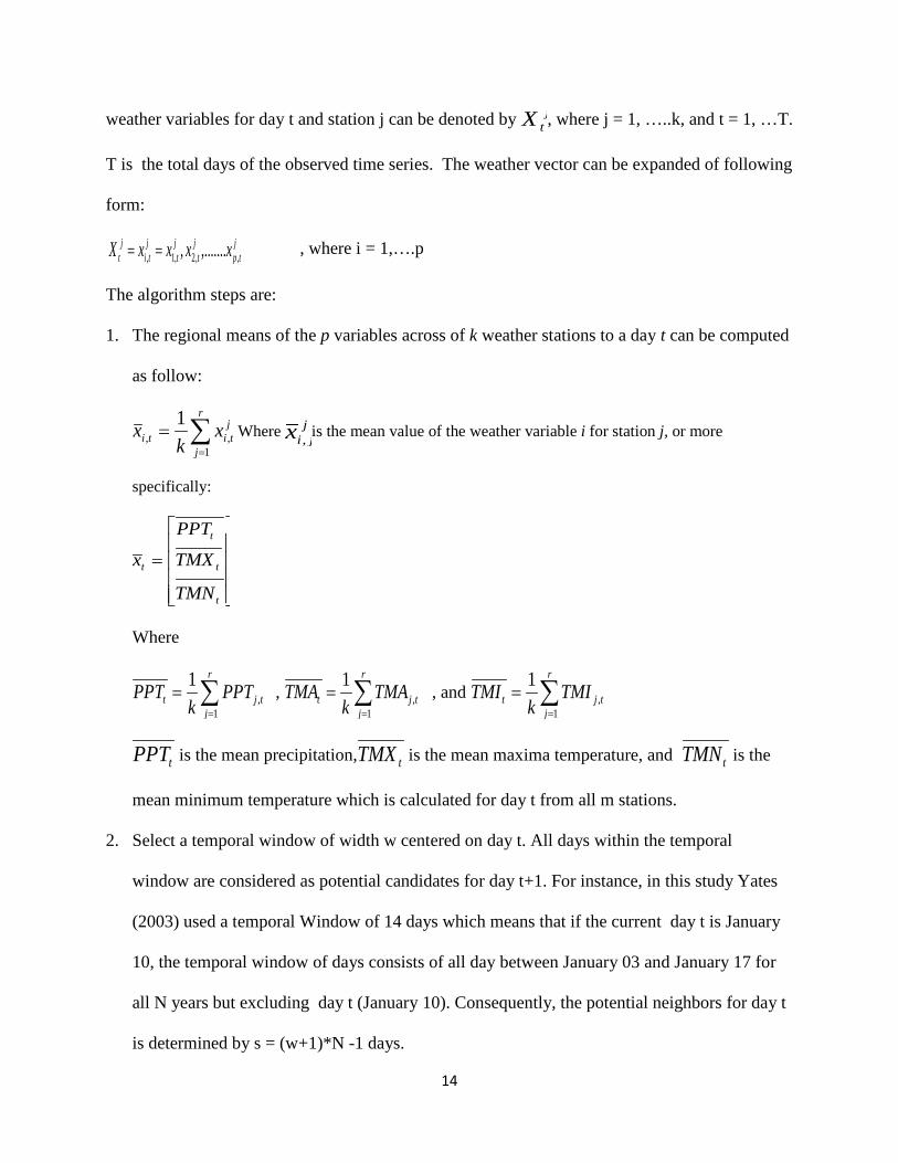
weather variables for day t and station j can be denoted by jtX , where j = 1, …..k, and t = 1, …T.

T is the total days of the observed time series. The weather vector can be expanded of following

form:

jtp

jt

jt

jti

jt xxxxX ,,2,1, ,.......,== , where i = 1,….p

The algorithm steps are:

1. The regional means of the p variables across of k weather stations to a day t can be computed

as follow:

∑=

=r

j

jtiti x

kx

1,,

1 Where j

jix , is the mean value of the weather variable i for station j, or more

specifically:

=

t

t

t

t

TMN

TMX

PPT

x

Where

∑=

=r

jtjt PPT

kPPT

1,

1, ∑

=

=r

jtjt TMA

kTMA

1,

1, and ∑

=

=r

jtjt TMI

kTMI

1,

1

tPPT is the mean precipitation, tTMX is the mean maxima temperature, and tTMN is the

mean minimum temperature which is calculated for day t from all m stations.

2. Select a temporal window of width w centered on day t. All days within the temporal

window are considered as potential candidates for day t+1. For instance, in this study Yates

(2003) used a temporal Window of 14 days which means that if the current day t is January

10, the temporal window of days consists of all day between January 03 and January 17 for

all N years but excluding day t (January 10). Consequently, the potential neighbors for day t

is determined by s = (w+1)*N -1 days.

15

3. For each day of potential neighbors computes mean vectors across r stations. For this end,

the equations given in the step1 are used.

4. Compute the covariance matrix, tCov for day t, using the data block sxp.

5. The weather on the first day t (e.g. January) comprising all p variables at r stations is

randomly chosen from set of all January 1 values of the historic record of N years; which

means that all January 1 are candidate days with the same probability of selection. This is the

feature vector itF that constitutes the stochastically generated weather for day t of year i

given for each station. The algorithm continues with the next day, t+1.

6. Mahalanobis distances id are computed between mean vector of the current day’s weather,

tx and the mean vector ix for day i where i = 1,…..s . Then the distance can be computed

through the following expression:

)() 1itt

Titi xxCovxxd −−= −

Where T is the transpose of the vector , i =1, ……s, and 1−tCov is the inverse of the

covariance matrix.

The distances are sorted in order ascending and the first K nearest neighbors are retained.

7. In this study, a heuristic method for choosing K was used, where sK = . The first K-

nearest neighbors is determined to be retained for resampling out of the total s.

8. A probability metric with weight function which assigns weights to each of the K-nearest

neighbors is compute by the following expression:

∑=

= K

i

j

i

jw

1/1

/1

16

A high weight is assigned to the neighbor with smallest distance while the least weight is

assigned the largest distance. Likewise, the cumulative probability can be estimated as:

∑=

=j

iij wp

1

9. Estimate, using the cumulative probability metric jp , the nearest neighbor of the current day

(t+1). First, generate a random number, )1,0(⊂z , for a p1< z < pk the day j (t+1), to the

distance dj , is selected for which z is closest to pj. On the other hand, if kPz ≤ , then t+1 day

corresponding to distance dk is selected. If 1pz ≥ , the day t+1 corresponding to distance d1 is

selected. Finally, the steps 6 through 9 are repeated to generate as many days of synthetic

data are required for the simulation.

In addition, to generate subsets of years for each week, a temporal probabilistic resampling

scheme was introduced in this study. The K-nn algorithm model was used to simulate daily

precipitation, maximum and minimum temperature at stations located in the Rocky Mountains

region and the central Midwest of the United States (Figure 5). Statistics analysis such as

correlation between variables, means, standard deviations, etc were carried out in order to assess

the performance of the model. In order to illustrate part of the results obtained in this study, the

figure 6 is presented. It shows the variation of the total precipitation over time series of 100 years

in which it is noted that the changes for April and May were the biggest with decreasing of the

precipitation in last decades of time series studied ( 90-100 mm first decades to 50-60 mm last

decades) . January and June present the smallest decline in the last decades for whole the

simulation period. On the other hand, in the same figure (on the right), the behavior of the daily

average temperature (weighted average of minimum and maximum temperature) can be seen. It

is clearly observed that in the long term the temperature increases for April and May in the range

17

of +2.7 oC and +3oC over all time period. Finally, it is shown that this technique simulates the

weather sequences at different stations, with a good performance in reproduce the spatial and

temporal statistics and a successful generation of climate change scenarios through the strategies

used to adapt the K-nn (strategic resampling ).

Figure 5. Study area and two focus regions with their weather stations used to apply the algorithm. 114198 in region 4 and 52281 in region 7 stations were used to illustrate the results. Yates et al (2003).

Figure 6. Total monthly precipitation for 100 years times for warmer-drier spring scenarios (left). Regional averaged time series (shaded lines), the 10-year moving averages (solids lines), and the linear trends for January, April, May, and June are shown with straight lines. Daily average temperature for the indicated months is shown in the right graph, with regionally averaged time series and the linear trend for the 100 years. Yates et al (2003).

18

Ghosh and Mujumdar (2006) generated future climate scenarios for rainfall by statistical

downscaling over state Orissa located on the east coast of India. In this study, the method

developed is based on a linear regression model to compute the precipitation using Global

Climate Model (GCM) outputs. Mean sea- level pressure and geo potential height of this GCM

were used as variables to regression. On the other hand, the Coupled Global Climate Model

(CGCM2) developed by the Canadian Center was used in this research. The IPCC-IS92a

scenario is considered in the model for which the variation of green-house gases forcing belongs

to the historical data from 1900 to 1990, with a rate increase of 1 % per year which is considered

to continue until 2100. First, the methodology consists in performing a statistical procedure

called Principal Component Analysis (PCA) in order to reduce the dimensionality of the

variables considered. It allows to indentify the multidimensional variables and to transfer to a

group of uncorrelated variables, those correlated. Likewise, the fuzzy clustering method was

used to classify the main variables indentified by PCA, and for the regression analysis, the fuzzy

cluster membership values were used, indicating that the regression models were modified for a

seasonal/periodic component different for months. Additionally, for future rainfall scenario, the

method assumes that the regression relationship will not change in the future time. On the other

hand, to carry out the regression analysis, monthly rainfall data from 1950 to 2003 was used.

The projections estimated for the future rainfall based on IPCC-IS92a scenario indicate that is

probably the increase of extreme hydrological events in Orissa in future such as is shown in

figure 7 and 8. For instance, it is noted that for wet periods the precipitation increases on the time

series period considered while for dry period the precipitation decreases considerably. Also, it is

suggested that the methodology developed in this study can be used to simulate precipitation at

regional scale and therefore also can be used for assessing climate change impacts.

19

Figure 7. Box-plot for monthly predicted rainfall. Figure 8. Predicted rainfall for wet (a) and dry (b) periods Ghosh(2006). On the other hand, the reality of many places in the world is the lack of weather stations with

historical records and other cases, it is limited, resulting difficult the application of the

downscaling methods from GCMs. However, several statistical methods have been applied for

some researchers to generate time series data for precipitation and temperature fundamentally, so

that it is possible to apply future climate scenarios and to assess the climate change impacts in a

specific region. A conditional generation method (CGM) based was applied to generate monthly

precipitation time series for the upper Blues Nile Basin in Ethiopia ( Kim and Kaluarachchi,

2008). The method consists in determining the conditional occurrence probability of a given

event. The joint probability density should be uniformly distributed if the probability of

occurrence of given variable at current month is independent of event of previous months. The

CGM was validated comparing with others statistical method such inverse transformation of the

cumulative density function and autoregressive processes (stochastic method first –order Markov

process). Furthermore, in this study, a time series of 100 years of six GCMs were used to

evaluate the change in precipitation for which only the emission scenario A2 was selected. The

main characteristics of this scenario is that it is used for mid to high range of emission, with

high CO2 concentrations, increase of the global population and energy consumption (IPCC,

2001). From GCMs, a percent change of monthly precipitation for each grid was estimated.

20

These changes were spatially downscaled to the weather stations considered in this study; for this

end, the triangular cubic interpolation method was used. In general, the results in this research

showed the conditional generation method reproduced reliable historical precipitation being even

more accurate than other methods applied which means that the historical spatial correlation at

stations can be conserved by CGM used. On the other hand, changes in the precipitation were

estimated for upper Nile basin indicating variations of 47 % in dry, 5% in wet, and 6 % in mild

seasons. Figure 9 shows the changes of precipitation (in percentage) in the area study estimated

for the six GCMs.

Figure 9. Spatial Distribution of annual precipitation changes (%) by the 2050s for Six GCMs: (a) CCSR, (b) CGCM, (c) CSIRO, (d) ECHAM, (e) GFDL, and (f) HADCM. (Kim and Kaluarachchi, 20008)

It is also necessary to indicate that in chapter 10 of IPCC (2001) can be found a description and

evaluation of statistical and dynamical downscaling from GCMs. Likewise, some comparisons

both techniques have been carried out. For instance, Murphy (1999) compared a statistical

downscaling based on regression against two dynamical downscaling techniques (RCM) over

Europe. Monthly mean precipitation and surface temperature anomalies were downscaled using

predictor sets. The results showed that the dynamical model estimated better the precipitation for

21

winter time while the statistical model was better to estimate the summertime temperature. Both

techniques showed important approximations; however, because of sophisticated dynamical

technique, it showed a better accuracy over the statistical method. Wilby et al. (2000) evaluated

hydrology response for the Animas River basin in Colorado, USA to statistical and dynamic

downscaling output for which daily precipitation and surface temperature were simulated. In this

study, the results indicate that both techniques showed a good performance for hydrological

modeling and these had greater skill than the course resolution data used to drive the

downscaling (raw NCEP output). In addition, for hydrological applications, the statistical

downscaling has the advantage of require few parameter and simple computations and the

dynamical model provides better estimates water balance than the raw and corrected reanalysis

output.

In general, all comparative studies described above showed that both methods have similar skills.

However, “the results may represent a further validation of the performance of RCMs, due to

that the statistical downscaling is based on observed relationships between predictands and

predictors” (IPCC, 2001).

4. Hydrology and Water Resources Modeling

Once, the GCMs data is downscaled, hydrology and water resources models are used in order to

assess the climate change impacts at local scale. The general procedure to evaluate climate

change impacts on the water resources are presented below:

• Precipitation, temperature, and solar radiation are extracted at the grid nodes from a

long time period of General Circulation Model simulations.

• A downscaling method is used to relate the regional GCM output to the surface

variables at the river basin scale.

22

• Using meteorological data and observed stream flows, a Hydrological model is

calibrated and validated, and it is forced with downscaled GCM scenarios to produce

stream flows sequences for different climates GCM scenarios.

• With the stream flow sequences produced, a water resource simulation model is used

to assess the climate scenarios and their impact on hydrology and the water resources

system

• Finally, evaluate some water management policies in order to mitigate the impacts

on water resources system.

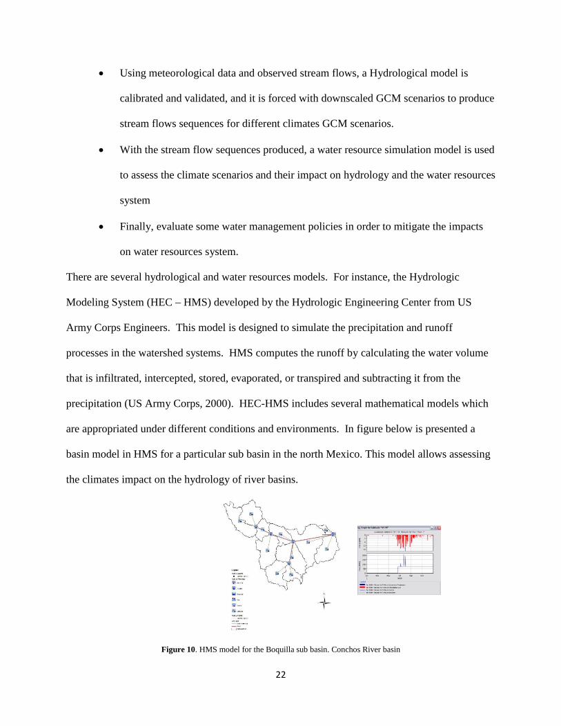
There are several hydrological and water resources models. For instance, the Hydrologic

Modeling System (HEC – HMS) developed by the Hydrologic Engineering Center from US

Army Corps Engineers. This model is designed to simulate the precipitation and runoff

processes in the watershed systems. HMS computes the runoff by calculating the water volume

that is infiltrated, intercepted, stored, evaporated, or transpired and subtracting it from the

precipitation (US Army Corps, 2000). HEC-HMS includes several mathematical models which

are appropriated under different conditions and environments. In figure below is presented a

basin model in HMS for a particular sub basin in the north Mexico. This model allows assessing

the climates impact on the hydrology of river basins.

Figure 10. HMS model for the Boquilla sub basin. Conchos River basin

23

On the other hand, Water Evaluation and planning System (WEAP) is an integrated water

resources model that simulates an entire water resources system that includes water demands,

groundwater, hydrology, water supply, water quality, and evaluate water management policies.

It has a hydrological module which is spatially continuous with areas configured as a set sub-

catchments that cover the entire river basin under study, considering them to be a complete

network such as rivers, reservoirs, channels, aquifers, demand points, etc. Likewise, this module

includes three methods to simulate catchment processes such as evapotranspiration, runoff,

infiltration, as a dynamic integrated rainfall-runoff model including various components of

hydrologic cycle.

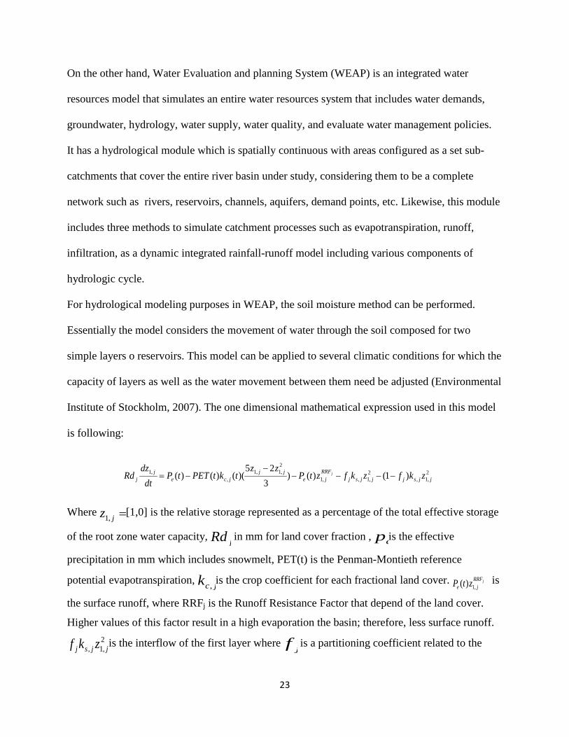
For hydrological modeling purposes in WEAP, the soil moisture method can be performed.

Essentially the model considers the movement of water through the soil composed for two

simple layers o reservoirs. This model can be applied to several climatic conditions for which the

capacity of layers as well as the water movement between them need be adjusted (Environmental

Institute of Stockholm, 2007). The one dimensional mathematical expression used in this model

is following:

2,1,

2,1,,1

2,1,1

,,1 )1()()

325

)(()()( jjsjjjsjRRF

jejj

jcej

j zkfzkfztPzz

tktPETtPdt

dzRd j −−−−

−−=

Where =jz ,1 [1,0] is the relative storage represented as a percentage of the total effective storage

of the root zone water capacity, jRd in mm for land cover fraction , ep is the effective

precipitation in mm which includes snowmelt, PET(t) is the Penman-Montieth reference

potential evapotranspiration, jck , is the crop coefficient for each fractional land cover. jRRFje ztP ,1)( is

the surface runoff, where RRFj is the Runoff Resistance Factor that depend of the land cover.

Higher values of this factor result in a high evaporation the basin; therefore, less surface runoff. 2,1, jjsj zkf is the interflow of the first layer where jf is a partitioning coefficient related to the

24

land cover type , soil, and topography that divides in both in vertically and horizontally flows,

jsk , is the hydraulic conductivity of saturated root zone in mm/time. The last term 2,1,)1( jjsf zkf−

is the deep percolation.

Now this model is being applied to assess the climate change impacts on the water resources in

the Rio Bravo basin, specifically in the Conchos River. Figure 11 shows some results of the

performance of the model. Temperature, precipitation, wind velocity, and relative humidity were

the inputs.

Figure 11. Observed and simulated runoff for a control station in the Conchos river basin. Period 20 years.

5. Conclusions

Based on the literature review, as consequence of climate changes, precipitation will decline in

lower and middle latitudes and it increases in some regions such as in the part of tropics and high

latitudes (simulated for 2080-2099 relative to 1980-1999). Soil moisture content decreases in

sub tropical and Mediterranean region. Runoff depends of the changes in precipitation; in this

sense, it is clearly reduced in central American and Europe and increases in high latitudes.

0

50

100

150

200

250

300

350

400

450

500

Jan-

80

Aug

-80

Mar

-81

Oct

-81

May

-82

Dec

-82

Jul-8

3

Feb-

84

Sep-

84

Apr

-85

Nov

-85

Jun-

86

Jan-

87

Aug

-87

Mar

-88

Oct

-88

May

-89

Dec

-89

Jul-9

0

Feb-

91

Sep-

91

Apr

-92

Nov

-92

Jun-

93

Jan-

94

Aug

-94

Mar

-95

Oct

-95

May

-96

Dec

-96

Jul-9

7

Feb-

98

Sep-

98

Apr

-99

Nov

-99

Vol

ume

in m

illio

n M

3

Month

Observed Simulated

25

Moreover, the annual evaporation increases over most oceans. Few indicators exists about the

change of groundwater recharge; however, in some studies evaluated, the groundwater recharge

will decrease considerably in the South West Africa and North-Eastern Brazil. Another

interesting aspect is the increase of risks of droughts and floods for sub tropical, low and mid

latitudes, and tropical and highs latitudes regions respectively.

Climate change will affect directly the water resources systems as is shown with results

described from GCMs models at global scale. Management and operation of hydraulic

infrastructures, irrigation methods, and water management practices will be affected. According

to IPCC, the area of land subject to increase of water stress due to climate change will be more

than double than those with decreasing stress.

On the other hand, for using the GCMs weather data to assess climate change impacts at local

scale is necessary and fundamental to downscale the global data. Statistical and dynamical

downscaling was reviewed. Statistical downscaling such as stochastic weather generators and

regression models has been used by several studies. Dynamic downscaling develops and uses a

regional climate model (RCM) with the course GCM data used as boundary conditions.

According to several studies, both techniques showed great skill to carry out the downscaling

task; however, dynamic downscaling requires of huge amount of computational resources and

take long time for the simulations.

Finally, the hydrology and water resources models are tools very important to evaluate climate

change impacts in the future at local scale. Many of them use mathematical models to represent

the behavior the runoff, groundwater, and climatic parameters.

26

References Castro, C., R.A. Pielke, and G. Leoncini, 2005. Dynamical Downscaling: Assessment of value

retained and added using the Regional Atmospheric Modeling System (RAMS). Journal of Geophysical Research, vol. 110, D05108.

Chong –yu, X., 1999. From GCMs to River Flow: A Review of Downscaling Methods and Hydrologic Modeling Approach. Progress in Physical Geography 23, 2: 229-249.

Ghosh, S. and P.P. Mujumdar, 2006. Future Rainfall Scenario over Orissa with GCM Projections by Statistical downscaling. Current Science, 90(3): 396-404.

Intergovernmental Panel on Climate Change (IPCC), 2008: Climate Change and Water. IPCC technical paper VI. http://www.ipcc.ch/ipccreports/tp-climate-change-water.htm

Intergovernmental Panel on Climate Change (IPCC), 2001: Climate Change 2001. Impacts, Adaption and Vulnerability. “Hydrology and Water Resources” http://www.ipcc.ch/ipccreports/tar/wg2/index.htm

Intergovernmental Panel on Climate Change (IPCC), 2001: The Scientific Basis. “Regional Climate Information – Evaluation and Projections”.

http://www.ipcc.ch/ipccreports/tar/wg1/index.htm Intergovernmental Panel on Climate Change (IPCC), 2008. About Stochastic Weather

Generators. http://www.ipcc-data.org/ddc_weather_generators.html

Kim, U., J.J. Kaluarachchi and V.U. Smakhtin, 2008. Generation of Monthly Precipitation under Climate Change for The Upper Blue Nile River Basin, Ethiopia. Journal of the American Water Resources Association 44(5): 1231-1247.

Murphy, J.M., 1999. An evaluation of Statistical and Dynamical Techniques for downscaling local climate. J. Climate, 12, 2256-2284.

Richardson, C.W., 1981. Stochastic Simulation of Daily Precipitation, Temperature, and Solar Radiation. Water Resources Research, 17( 1):182-190.

Stockholm Environment Institute's Boston Center, 2007. Water Evaluation and Planning System, WEAP.

US Army Corps of Engineers, 2000. Hydrologic Modeling System HEC-HMS. Technical Reference Manual.

Wilby, R.L., L.E. Hay, W.J. Gutowski, R.W. Arritt, E.S. Takle, Z. Pan, G.H. Leavesley and M.P. Clark, 2000. Hydrological responses to dynamically and statistically downscaled climate model output. Geophysical Research Letters., 27(8): p1199-1202.

Wilby, R.L., and T.M.L Wigley, 1997. Downscaling General Circulation Model Ouput: Review of Methods and Limitations. Progress in Physical Geography 21, 4: 530-548.

Yates, D., S. Gangopadhyay, B. Rajagoplan and K. Strzepek, 2003. A Technique for Generating Regional Climate Scenarios using a Nearest –Neighbor Algorithm. Journal Water Resources Research 39(7): SWC 7-1 - 7-15.