Embed Size (px)
Citation preview

Omotayo Babawande Adeboye
Trang Minh Duong
Climate Change Impacts on the Stability of Small Tidal Inlets

CLIMATE CHANGE IMPACTS ON THE STABILITY OF SMALL TIDAL INLETS


CLIMATE CHANGE IMPACTS ON THE STABILITY OF SMALL TIDAL INLETS
DISSERTATION
Submitted in fulfilment of the requirements of
the Board for Doctorates of Delft University of Technology
and
of the Academic Board of the UNESCO-IHE Institute for Water Education
for
the Degree of DOCTOR
to be defended in public
on Tuesday, 1st December 2015, at 15:00 hours
in Delft, the Netherlands
by
Trang Minh Duong
Master of Science, UNESCO-IHE, Delft, the Netherlands
born in Hanoi, VietNam

This dissertation has been approved by the promoters: Prof. dr. ir. J. A. Roelvink and Prof.dr. R.W.M.R.J.B. Ranasinghe Composition of the Doctoral Committee: Chairman Rector Magnificus, TU Delft Vice-Chairman Rector, UNESCO-IHE Prof. dr. ir. J.A. Roelvink UNESCO-IHE/Delft University of Technology, Promotor Prof. dr. R.W.M.R.J.B. Ranasinghe UNESCO-IHE/Australian National University, Promotor Independent members: Dr. S. Weesakul Asian Institute of Technology/HAII, Bangkok, Thailand Prof. dr. M. Larson Lund University, Sweden Prof. dr.ir. A.E. Mynett UNESCO-IHE/Delft University of Technology Prof. dr.ir. Z.B. Wang Delft University of Technology Prof. dr. D.P. Solamatine Delft University of Technology, reserve member
CRC Press/Balkema is an imprint of the Taylor & Francis Group, an informa business © 2015, Trang Minh Duong
All rights reserved. No part of this publication or the information contained herein may be reproduced, stored in a retrieval system, or transmitted in any form or by any means, electronic, mechanical, by photocopying, recording or otherwise, without written prior permission from the publishers. Although all care is taken to ensure the integrity and quality of this publication and information herein, no responsibility is assumed by the publishers or the author for any damage to property or persons as a result of the operation or use of this publication and or the information contained herein. Published by: CRC Press/Balkema PO Box 11320, 2301 EH Leiden, The Netherlands e-mail: [email protected] www.crcpress.com – www.taylorandfrancis.com ISBN 978-1-138-02944-6 (Taylor & Francis Group)

This research was supported by the DUPC-UPARF cooperation program between the Dutch Foreign Ministry (DGIS) and UNESCO-IHE and the AXA Research Fund.


vii
ABSTRACT
The coastal zones in the vicinity of tidal inlets, which are commonly utilized for navigation, sand
mining, waterfront developments, fishing and recreation, are under particularly high population
pressure. The intensive population concentration and excessive natural resources exploitation in
these areas could lead to biodiversity loss, destruction of habitats, pollution, as well as conflicts
between potential uses, and space congestion problems, which will only be exacerbated by
foreshadowed climate change (CC). Although a very few recent studies have investigated CC
impacts on very large tidal inlet/basin systems, the nature and magnitude of CC impacts on the
more commonly found small tidal inlet/estuary systems remains practically un-investigated to date.
These relatively small estuaries/lagoons (also known as "bar-built" or "barrier" estuaries, and
hereon referred to as Small Tidal Inlets or STIs) are common along wave-dominated, microtidal
mainland coasts comprising about 50% of the world's coastline.
Due to their common occurrence in the tropical and sub-tropical zones, most STIs are found in
developing countries, where data availability is generally poor (i.e. data poor environments) and
community resilience to coastal change is low. Furthermore, STI environs in developing countries
especially host a number of economic activities (and thousands of associated livelihoods) which
contribute significantly to the national GDPs. The combination of pre-dominant occurrence in
developing countries, socio-economic relevance and low community resilience, general lack of
data, and high sensitivity to seasonal forcing makes STIs potentially very vulnerable to CC impacts
and thus a high priority area of research. This study was therefore undertaken with the overarching
objective of (a) developing methods and tools that can provide insights on potential CC impacts on
STIs, and (b) demonstrating their application to assess CC impacts on the main types of STIs.
Throughout this Thesis, 3 case study STIs representing the 3 main STI Types are used:
- Negombo lagoon, Sri Lanka: Permanently open, locationally stable inlet (Type 1)
- Kalutara lagoon, Sri Lanka: Permanently open, alongshore migrating inlet (Type 2)
- Maha Oya river, Sri Lanka: Seasonally/Intermittently open, locationally stable inlet (Type 3)
To circumnavigate the inability of contemporary process based coastal area morphodynamic
models to accurately simulate the morphological evolution of STIs over typical CC impact

viii
assessment time scales (e.g. 100 yrs) with concurrent tide, wave and riverflow forcing, 2 different
snap-shot modelling approaches for data poor and data rich environments are proposed. The data
poor approach uses schematized flat bed bathymetries that follow real world STIs and CC forcing
derived from freely available coarse resolution global models while the data rich approach requires
detailed bathymetries and downscaled CC forcing. Furthermore, to enable rapid assessments of CC
impacts on STI stability, particularly to aid frontline coastal zone managers/planners, a reduced
complexity model is developed based on existing knowledge and physical formulations. The
model, which is capable of simulating 100 years in under 3 seconds on a standard PC, provides
predictions of STI stability based on the Bruun inlet stability criterion r (= P/M; where P = tidal
prism (m3) and M = annual longshore transport (m3/yr)).
Based on process based snap-shot model applications under contemporary forcing, a clear link
between STI Type and r is established (Table 1).
Table 1. Classification scheme for inlet Type and stability conditions.
All 3 modelling approaches show that Type 1 and Type 3 STIs will not change Type by the year
2100. For Type 2 STIs, the data poor approach suggests a Type change to Type 1 when CC results
in a decreased annual longshore sediment transport, while the other two approaches predict no
Type change under any CC forcing scenario. However, the results of the data rich approach and the
reduced complexity model are likely to be more reliable due to the use of more accurate
bathymetric data and site specific, downscaled CC forcings therein.
Although CC driven STI Type changes appear to be rather unlikely in the 21st century, model
results do show that CC is likely to change the level of stability of STIs, indicated by significant
future changes of the r value from its present value. At Type 1 STIs, future CC driven
increases/decreases in longshore sediment transport may result in decreases/increases in their level
Inlet Type r =P/M Bruun Classification
Type 1
> 150 Good 100 - 150 Fair 50 - 100 Fair to Poor 20 - 50 Poor
Type 2 10 - 20 Unstable
(open and migrating)
Type 2/3 5 - 10 Unstable
(migrating or intermittently closing)
Type 3 0 - 5 Unstable
(intermittently closing)

ix
of stability. At Type 2 and Type 3 STIs concurrent increases (decreases) in longshore sediment
transport and decreases (increases) in riverflow may result in decreasing (increasing) the level of
inlet stability. Sea level rise (SLR) appears not to be the main driver of change in the level of STI
stability, with CC driven variations in wave direction emerging as the major driver of potential
change in STI stability.
For future CC impacts assessment at STIs, an initial assessment using the reduced complexity
model is recommended. If Type changes are predicted at any time (or if r drops below 10 for a
Type 2 STI), or if specific insights (e.g. migration distance at Type 2 STIs, inlet closure time at
Type 3 STIs) are desired, then it is essential that the (data poor or data rich, depending on which is
feasible in the study area) process based snap-shot modelling approach be adopted.

x
SAMENVATTING
Kustgebieden in de nabijheid van zeegaten, die vaak worden gebruikt voor scheepvaart,
zandwinning, waterfront ontwikkeling, visserij en recreatie, kennen een bijzonder hoge
bevolkingsdruk. De hoge bevolkingsdichtheid en het verregaande gebruik van het natuurlijke
system in deze gebieden kan een verlies van biodiversiteit, vernietiging van habitats en vervuiling
tot gevolg hebben alsmede leiden tot conflicten in gebruik en overbelasting van de ruimte. Deze
aspecten worden bovendien versterkt door de voorspelde klimaatverandering (KV). Hoewel een
aantal recente onderzoeken de invloed van KV op grote zeegat/bekken systemen hebben
onderzocht, is de aard en de omvang van de KV op kleine zeegat/bekken systemen tot op heden
nauwelijks onderzocht. Deze relatief kleine estuaria/lagunes (ook wel ‘bar built’ of ‘barrier’
estuaria genoemd, hierna aangeduid als Kleine Zeegat Systemen of KZS) zijn wijdverspreid langs
golf-gedomineerde, micro-getijde kusten langs de continenten, die grofweg 50 % van ‘s werelds
kustlijn beslaan.
Doordat deze KZS veel voorkomen in tropische en subtropische gebieden, zijn de meeste KZS
gelegen in ontwikkelingslanden waar de beschikbaarheid van gegevens over het algemeen laag is
(zgn. data schaarse omgevingen) en er weinig veerkracht van de lokale gemeenschap is voor
kustverandering. Bovendien huisvesten de gebieden rondom KZS, met name in
ontwikkelingslanden, een aantal economische activiteiten die aanzienlijk bijdragen aan het bruto
binnenlands product. De combinatie van dit voornamelijk voorkomen in ontwikkelingslanden, het
sociaaleconomische belang, de beperkte veerkracht van de lokale bevolking, het gebrek aan
gegevens en de gevoeligheid voor seizoensvariatie in de aandrijvende krachten zorgt ervoor dat de
KZS in potentie zeer kwetsbaar zijn voor KV wat dit een onderzoeksgebied maakt met een hoge
prioriteit. Dit onderzoek heeft derhalve de volgende overkoepelende onderzoeksdoelen: a) het
ontwikkelen van methoden en instrumenten die inzicht kunnen geven in de mogelijke impact van
KV op KZS, en b) het aantonen van de bruikbaarheid van deze methoden en instrumenten om de
impact van KV op de belangrijkste typen KZS te beoordelen.
In deze dissertatie zijn 3 casestudy's van KZS onderzocht, die kenmerkend zijn voor de 3
belangrijke typen KZS:
- Negombo lagoon, Sri Lanka: Permanent open, plaatsvast zeegat (Type 1)

xi
- Kalutara lagoon, Sri Lanka: Permanent open, kustlangs verplaatsend zeegat (Type 2)
- Maha Oya river, Sri Lanka: Seizoensgebonden/afwisselend open, plaatsvast zeegat (Type 3)
Om de beperkingen van de huidige proces gebaseerde kustmorfodynamica modellen om accuraat
de morfologische verandering van KZS over de tijdschaal van KV (bv. 100 jaar) met de
samenhangende aandrijvende krachten van getijde, golven en de rivier te overkomen, zijn twee
verschillende snapshot model benaderingen voorgesteld voor zowel data schaarse en data rijke
gebieden. De data schaarse benadering maakt gebruik van geschematiseerde vlakke
bodemliggingen die werkelijke KZS volgen en KV aandrijvende krachten die zijn afgeleid uit vrij
verkrijgbare, wereld dekkende modellen met een grove resolutie. De data rijke benadering vereist
daarentegen gedetailleerde bodemligging en een beschrijving van de aandrijvende krachten van KV
op kleinere schaal. Daarnaast is een model benadering met gereduceerde complexiteit ontwikkeld,
gebaseerd op bestaande kennis en fysieke relaties, om een snelle beoordeling van KV impact op
KZS mogelijk te maken, in het bijzonder om praktijkgerichte kustzone managers/planners te
helpen. Het model, waarmee het mogelijk is om 100 jaar vooruit te voorspellen met een rekentijd
van 3 seconden op een standaard PC, geeft voorspellingen van de stabiliteit van KZS door gebruik
te maken van het Bruun zeegat stabiliteits criterium r (= P/M; waarbij P = getijde prisma (m3) en M
= jaarlijks kustlangs transport (m3/jaar) is).
Door gebruik te maken van de proces gebaseerde snapshot model toepassingen met hedendaagse
forcering is een duidelijke link vastgesteld tussen het type KZS en parameter r (Tabel 1).
Tabel 1. Classificatie schema voor het type zeegat en de stabiliteitscondities.
Alle drie de model benaderingen laten zien dat KZS van Type 1 en Type 3 niet van type zullen
veranderen voor het jaar 2100. Voor KZS van Type 2 geeft de data schaarse aanpak aan dat het
type van het KZS verandert naar Type 1 als KV leidt tot een afname van het jaarlijks kustlangse
Type zeegat r =P/M Bruun Classificatie
Type 1
> 150 Goed 100 - 150 Redelijk 50 - 100 Redelijk tot Matig 20 - 50 Matig
Type 2 10 - 20 Instabiel
(open en kustlangs verplaatsend)
Type 2/3 5 - 10 Instabiel
(kustlangs verplaatsend of afwisselend sluitend)
Type 3 0 - 5 Instabiel
(afwisselend sluitend)

xii
sediment transport, terwijl de overige twee modelbenaderingen geen type verandering voorspellen
onder elk van de KV scenario’s. Hierbij moet worden aangemerkt dat de resultaten van het data
rijke model en het gereduceerde complexiteit model waarschijnlijk betrouwbaarder zijn omdat deze
gebruik maken van nauwkeurigere gegevens van de bodemligging en gebied specifieke, KV
gerelateerde aandrijvende krachten op kleinere schaal.
Hoewel het onwaarschijnlijk lijkt dat KV leid tot verandering van het type van KZS in de 21st
eeuw, laten de model resultaten zien dat KV wel de mate van stabiliteit van KZS verandert, wat
zichtbaar is als een significante verandering in de r waarde ten opzichte van de huidige waarde.
Voor Type 1 KZS kan een KV gedreven toename/afname van het kustlangse sediment transport
leiden tot een afname/toename van het stabiliteitsniveau. Voor KZS van Type 2 en Type 3 kunnen
gelijktijdige toename (afname) in het kustlangs sediment transport en afname (toename) in de
rivierafvoer leiden tot een afnemende (toenemende) stabiliteit van het zeegat. Zeespiegelstijging
lijkt niet de belangrijkste drijvende kracht voor het stabiliteitsniveau van de het KZS, maar KV
gedreven veranderingen in de golfrichting kwamen naar voren als de belangrijkste drijvende kracht
voor potentiele verandering in de stabiliteit van KZS.
Voor een toekomstige beoordeling van de impact van KV bij KZS, wordt aangeraden een eerste
beoordeling te maken met het model met gereduceerde complexiteit. Indien verandering van het
zeegat type wordt voorspeld gedurende de looptijd van de voorspelling (of indien r waardes onder
de 10 komen voor KZS van Type 2), of indien specifieke inzichten benodigd zijn (bv. de
kustlangse verplaatsingsafstand bij KZS van Type 2, of de tijd tot afsluiting van het zeegat bij KZS
van Type 3,), dan is het essentieel om de (data schaarse of data rijke, afhankelijk van wat haalbaar
is in het interesse gebied) proces gebaseerde snapshot model benadering toe te passen.
This abstract is translated from English to Dutch by Dr.ir. Matthieu de Schipper, Faculty of Civil Engineering and Geosciences, Delft University of Technology.

xiii
Contents 1. Introduction .................................................................................................... 1
1.1. Problem Statement ................................................................................................................1 1.2. Objective and Research questions ......................................................................................... 3
2. Assessing climate change impacts on the stability of small tidal inlet systems: why and how? ......................................................... 6 2.1. Introduction ........................................................................................................................... 6 2.2. Stability of Small Tidal Inlets .................................................................................................. 8 2.3. Potential Climate Change drivers of Small Tidal Inlet stability .............................................. 12 2.4. Quantifying Climate Change impacts on the stability of Small Tidal Inlets ........................... 16 2.5. Discussion .............................................................................................................................. 25 2.6. Summary and Conclusions ..................................................................................................... 26
3. Assessing climate change impacts on the stability of small tidal inlets in data poor environments ................................................... 30 3.1. Introduction ........................................................................................................................... 30 3.2. Methodology ......................................................................................................................... 30 3.3. Results ................................................................................................................................... 40 3.4. Conclusions ............................................................................................................................ 63
4. Assessing climate change impacts on the stability of small tidal inlets in data rich environments ..................................................... 67 4.1. Introduction ........................................................................................................................... 67 4.2. Dynamic downscaling ............................................................................................................ 69 4.3. Regional/catchment scale coastal forcing models ................................................................ 70 4.4. Coastal Impact modelling ...................................................................................................... 72 4.5. Conclusions ............................................................................................................................ 86
5. A reduced complexity model to obtain rapid predictions of climate change impacts on the stability of small tidal inlets ............................ 89 5.1. Introduction ........................................................................................................................... 89 5.2. Governing processes .............................................................................................................. 90 5.3. The model .............................................................................................................................. 92 5.4. Model applications and Results ............................................................................................. 95 5.5. Conclusions ............................................................................................................................ 105
6. General Conclusions ........................................................................................ 108

xiv

Trang Minh Duong Climate Change impacts on the stability of Small Tidal Inlets
1
CHAPTER 1
INTRODUCTION
1.1 Problem statement
A tidal inlet is defined as a waterway connection between the ocean and a protected embayment, it
may be a bay, lagoon, or estuary through which tidal and other currents flow (Carter, 1988). Thus,
it is through the inlet that the exchange of water, sediment and pollutants occur between the ocean
and the lagoon/estuary.
Tidal inlets are of great societal importance as they are often associated with ports and harbours,
industry, tourism, recreation and prime waterfront real estate. Tidal inlets are also among the most
morphologically dynamic regions in the coastal zone (Kjerfve, 1994; Nicholls et al., 2007;
Ranasinghe et al., 2013). The complex feedbacks between system forcing and response in these
areas result in ongoing spatial and temporal variations in system characteristics which are of great
scientific interest and continue to be the focus of numerous scientific studies (O'Brien, 1931;
Escoffier, 1940; Bruun, 1978; Aubrey and Weishar, 1988; Prandle, 1992; Ranasinghe and
Pattiaratchi, 2003; FitzGerald et al., 2008; Bertin et al., 2009; Lam, 2009; van der Wegen et al.,
2010; Bruneau et al., 2011; Tung, 2011; Nahon et al., 2012; Dissanayake et al., 2012; Ranasinghe
et al., 2013).
Tidal inlet behaviour is governed by the delicate balance of oceanic processes such as tides, waves
and mean sea level (MSL), and fluvial processes such as riverflow and fluvial sediment fluxes.
Alarmingly, all of these processes can be affected by climate change (CC) processes, which may
result in severe negative physical impacts such as erosion of open coast beaches adjacent to the
inlet and/or estuary margin shorelines, permanent or frequent inundation of low lying areas on
estuary margins, eutrophication, and toxic algal blooms etc. Furthermore, CC driven changes in

Trang Minh Duong Climate Change impacts on the stability of Small Tidal Inlets
2
forcing may affect the stability of the inlet itself. For example, a permanently open, locationally
stable inlet may evolve into an alongshore migrating, intermittently closing inlet or a seasonally
closing, locationally stable inlet may evolve into a permanently open, alongshore migrating inlet.
Such changes in inlet condition are highly likely to affect navigability and estuary/lagoon water
quality leading to significant socio-economic, environmental and ecological losses.
Although a very few recent studies have investigated CC impacts on very large tidal inlet/basin
systems (e.g. Dissanayake et al., 2012; van der Wegen, 2013), the exact nature and magnitude of
CC impacts on the more commonly found small tidal inlet/estuary systems remains practically un-
investigated to date. These relatively small estuaries/lagoons, which are also known as "bar-built"
or "barrier" estuaries (hereafter referred to as Small Tidal Inlets or STIs for convenience) are
common along wave-dominated, microtidal mainland coasts comprising about 50% of the world's
coastline (Ranasinghe et al., 2013). While the exact number of STIs present around the world is
unknown, it is likely to run into thousands with predominant occurrence in tropical and sub-tropical
regions (e.g. India, Sri Lanka,Vietnam, Florida (USA), South America (Brazil), West and South
Africa, and SW/SE Australia). STIs generally have little or no intertidal flats, backwater marshes or
ebb tidal deltas. The barrier of these systems is usually a sand spit that is connected to the
mainland, in contrast to a barrier island where the barrier is completely separated from the
mainland. STI systems usually contain inlet channels that are less than 500m wide connected to
relatively shallow (average depth < 10 m) estuaries/lagoons with surface areas less than 50 km2.
There are 3 main STI Types:
- Permanently open, locationally stable inlets (Type 1)
- Permanently open, alongshore migrating inlets (Type 2)
- Seasonally/Intermittently open, locationally stable inlets (Type 3)
The most severe CC impact on a given STI would be a change in Type. This could potentially
affect all or most economic and social activities centred on the STI that had developed over time
based on the expectation that the general morphological behaviour of the STI will remain
unchanged. For example, if a Type 1 system of which the lagoon is used as an anchorage for sea
going vessels changes into a Type 3 system, it may no longer be possible to operate as an efficient
anchorage. A less severe, but still potentially very socio-economically damaging CC impact would
be a significant change in the level of stability of an STI (as per the Bruun inlet stability criterion
r = P/M; where P = tidal prism (m3) and M = annual longshore transport (m3/yr); Bruun, 1978),
while its Type remains unchanged. For example, if the level of stability of the same example
Type 1 STI changes from 'good' ( r > 150) to 'poor' (20 < r < 50), although it will still remain as a

Trang Minh Duong Climate Change impacts on the stability of Small Tidal Inlets
3
Type 1 inlet, navigation through the inlet might become difficult and perilous, thus seriously
compromising its continued functionality as an efficient anchorage.
Due to their pre-dominant occurrence in tropical and sub-tropical zones, STIs usually experience a
strong seasonal cycle in system forcing comprising high and low riverflow/wave energy seasons
(monsoon/non-monsoon or winter/summer). Their common occurrence in the tropical and sub-
tropical zones also results in most STIs being found in developing countries, where data
availability is mostly poor (i.e. data poor environments) and community resilience to coastal
change is rather low compared to that in developed countries. Furthermore, STI environs in
developing countries especially host a number of economic activities (and thousands of associated
livelihoods) such as harbouring sea going fishing vessels, inland fisheries (e.g. prawn farming),
tourist hotels and tourism associated recreational activities which contribute significantly to the
national GDPs. The combination of pre-dominant occurrence in developing countries, socio-
economic relevance and low community resilience, general lack of data, and high sensitivity to
seasonal forcing makes STIs potentially very vulnerable to CC impacts and thus a high priority
area of research. This Thesis therefore entirely focusses on CC impacts on STIs.
1.2 Objective and Research questions
1.2.1 Objective
The overarching objective of this study is to (a) develop methods and tools that can provide
insights on potential CC impacts on STIs, and (b) to demonstrate their application to qualitatively
and quantitatively assess CC impacts on different types of STIs.
1.2.2 Research Questions
To achieve the above objective, this study will attempt to answer the following specific research
questions:
• Research Question 1: Can a process based coastal area model be used to assess CC impacts
on STIs?
• Research Question 2: Can an easy-to-use reduced complexity model be developed to
obtain rapid assessments of the temporal evolution of STI stability under CC forcing?
• Research Question 3: Is there a link between STI Type and the Bruun inlet stability
criterion (r = P/M; where P = tidal prism (m3) and M = annual longshore transport (m3/yr))
that could aid in classifying different STI responses to CC?

Trang Minh Duong Climate Change impacts on the stability of Small Tidal Inlets
4
• Research Question 4: Will CC change STI Type?
• Research Question 5: How will CC affect the level of stability of STIs?
• Research Question 6: What basic guidelines can be given to coastal zone managers on how
to assess CC impacts on STIs to inform CC adaptation strategies?
References
Aubrey, D. G. and Weishar, L., (Eds), 1988. Hydrodynamics and sediment dynamics of tidal inlets. Lecture Notes on Coastal and Estuarine Studies, 29. Springer-Verlag, New York. 456p.
Bertin, X., Fortunato, A.B., Oliveira, A., 2009. A modeling-based analysis of processes driving wave-dominated inlets. Continental Shelf Research, 29 (5–6), 819–834.
Bruneau, N., Fortunato, A.B., Dodet, G., Freire, P., Oliveira, A., Bertin, X., 2011. Future evolution of a tidal inlet due to changes in wave climate, sea level and lagoon morphology: O´bidos lagoon, Portugal. Continental Shelf Research 31, 1915–1930.
Bruun, P., 1978. Stability of tidal inlets – theory and engineering. Developments in Geotechnical Engineering. Elsevier Scientific, Amsterdam, 510p.
Carter, R. W. G., 1988. Coastal Environments. Academic Press. London. 617p.
Dissanayake P. K.., Ranasinghe, R., Roelvink, D., 2012. The morphological response of large tidal inlet/basin systems to sea level rise. Climatic Change, 113, 253-276.
Escoffier, F.F., 1940. The stability of tidal inlets. Shore and Beach, 8,111–114.
FitzGerald, D.M., Fenster, M.S., Argow, B.A., Buynevich, I.V., 2008. Coastal impacts due to sea-level rise. Annual Review of Earth and Planetary Sciences, 36, 601-647.
Kjerfve, B., 1994. Coastal Lagoon Processes. In: Kjerfve, B., (Ed), Coastal Lagoon Processes. Elsevier Science Publishers, Amsterdam, pp. 1-8.
Lam, N. T., 2009. Hydrodynamics and morphodynamics of a seasonally forced tidal inlet system. Ph.D. Thesis, Delft University of Technology.
Nahon, A., Bertin, X., Fortunato, A.B., Oliveira, A., 2012. Process-based 2DH morphodynamic modeling of tidal inlets: A comparison with empirical classifications and theories. Marine Geology, 291–294, 1–11, doi:10.1016/j.margeo.2011.10.001.
Nicholls, R.J., Wong, P.P., Burkett, V.R., Codignotto, J.O., Hay, J.E., McLean, R.F., Ragoonaden, S., Woodroffe, C.D., 2007. Coastal systems and low-lying areas. Climate Change 2007: Impacts, Adaptation and Vulnerability, Contribution of Working Group II to the Fourth Assessment Report of the Intergovernmental Panel on Climate Change, Cambridge University Press, Cambridge, UK.
O’Brien, M.P., 1931. Estuary and tidal prisms related to entrance areas. Civil Engineering 1(8), 738-739.
Prandle, D., 1992. Dynamics and Exchanges in Estuaries and the Coastal Zone. American Geophysical Union, Washington. 650p.
Ranasinghe, R., Pattiaratchi, C., 2003. The seasonal closure of tidal inlets: causes and effects. Coastal Engineering Journal, 45(4), 601-627.

Trang Minh Duong Climate Change impacts on the stability of Small Tidal Inlets
5
Ranasinghe, R., Duong, T.M., Uhlenbrook, S., Roelvink, D., Stive, M., 2013. Climate change impact assessment for inlet-interrupted coastlines. Nature Climate Change, 3, 83-87, DOI.10.1038/NCLIMATE1664.
Tung, T. T., 2011. Morphodynamics of Seasonally closed coastal inlets at the central coast of Vietnam. Ph.D. Thesis, Delft University of Technology.
van der Wegen, M., Dastgheib, A., Roelvink, J.A., 2010. Morphodynamic modeling of tidal channel evolution in comparison to empirical PA relationship. Coastal Engineering. 57, 827–837, doi:10.1016/j.coastaleng.2010.04.003.
van der Wegen, M., 2013. Numerical modeling of the impact of sea level rise on tidal basin morphodynamics, Journal of Geophysical Research, 118, doi:10.1002/jgrf.20034.

Trang Minh Duong Climate Change impacts on the stability of Small Tidal Inlets
6
CHAPTER 2
ASSESSING CLIMATE CHANGE IMPACTS ON THE STABILITY OF SMALL TIDAL INLET SYSTEMS: WHY AND HOW?
2.1 Introduction
Coastal zones have historically attracted humans and human activities due to their amenity,
aesthetic value and diverse ecosystems services, resulting in rapid expansions in settlements,
urbanization, infrastructure, economic activities and tourism. At present, approximately 23% of the
global population lives within 100km and less than 100m above sea level (Small and Nicholls,
2003). The coastal zones in the vicinity of tidal inlets, which are commonly utilized for navigation,
sand mining, waterfront developments, fishing and recreation, are under particularly high
population pressure. The intensive population concentration and excessive natural resources
exploitation in these areas could lead to biodiversity loss, destruction of habitats, pollution, as well
as conflicts between potential uses, and space congestion problems, which will only be exacerbated
by foreshadowed climate change. In the case of tidal inlets, the adjacent coastal zones will be
affected not only by CC driven variations in oceanic processes (e.g. Sea level rise, waves), but also
by CC driven variations in terrestrial processes (e.g. rainfall/runoff) (Ranasinghe et al., 2013). Any
negative impacts of CC on inlet environment are therefore very likely to result in large socio-
economic impacts.
Tidal inlets which connect an estuary/lagoon/river to the coast are commonly found throughout the
world. While the total number of inlets around the world is to date unquantified, it is likely to be
several tens of thousands (Carter and Woodroffe, 1994). Bruun and Gerritsen (1960) distinguish
three inlet classes based on their origin, as geological origin (also known as drowned river valleys);

Trang Minh Duong Climate Change impacts on the stability of Small Tidal Inlets
7
littoral origin such as openings through barrier islands, and hydrological origin where a river enters
the sea (directly or via an estuary/lagoon) (Figure 2.1).
Figure 2.1. Examples of the three main types of tidal inlets: (a) Golden Gate, California, USA (Geological origin or drowned river valley inlet); (b) Drum Inlet, North Carolina, USA (Littoral origin or barrier island inlet) ; (c) Maha Oya river inlet, Sri Lanka (Hydrological origin or bar-built/barrier estuary inlet) (sources: Google and Google earth images).
Geological origin inlets (e.g. The Golden Gate inlet, California, USA; Botany Bay inlet, Sydney,
Australia) are believed to have been formed by glacier-fed rivers scouring through bedrock on their
way to the ocean during the last Ice Age, when sea level was several hundred meters lower. Sea
level rise during the Holocene has resulted in the associated river valleys being slowly drowned,
forming large estuaries and wide, stable inlets.
Barrier island coasts are reported to comprise about 15% of the world’s coastlines (FitzGerald et
al., 2008). These coasts are formed by groups or chains of barrier islands and inlets (i.e. gaps in the
island chain) that mostly occur parallel to the mainland coast. Barrier islands are formed due to the
combined action of waves, winds and longshore current that result in the formation of thin strips of
land that are several meters above MSL. Barrier island coasts are usually separated from the
mainland by lagoons, marshes and/or tidal flats. While this type of inlet systems is found in every
continent except Antarctica, a vast majority is located along the US East coast and the Gulf of
Mexico, East and West coast of Alaska and East coast of South America (FitzGerald et al., 2008).
The third type of tidal inlets connects relatively small estuaries/lagoons, known as "bar-built" or
"barrier" estuaries, to the ocean (hereafter referred to as Small Tidal Inlets or STIs for
convenience). These are commonly found in wave-dominated, microtidal mainland (Ranasinghe et
al., 2013). Due to their pre-dominant occurrence in tropical and sub-tropical zones, these systems
usually experience a strong seasonal cycle in system forcing comprising high and low
a) b) c)

Trang Minh Duong Climate Change impacts on the stability of Small Tidal Inlets
8
riverflow/wave energy seasons (monsoon/non-monsoon or winter/summer). In some cases, wave
direction may also have a strong annual signal, particularly in monsoonal areas. As mentioned in
Chapter 1, due to their high vulnerability to CC impacts, understanding and quantifying CC
impacts on the stability of STIs is crucial. As a first step towards achieving that challenging goal,
this introductory Chapter aims to: (a) summarise potential CC impacts on the stability of STIs, (b)
conceptualise means by which the CC impacts maybe quantified using existing modelling tools,
and (c) propose ways forward to enable better quantification of CC impacts on STIs.
This Chapter is structured as follows. First a brief review of the stability of STIs is provided in
Section 2.2, followed by a summary of the CC processes (and their global projections) that may
affect STI stability in Section 2.3. Subsequently, in Section 2.4, the quantification of CC impacts
on STIs using currently available numerical modelling tools is discussed and two different
modelling frameworks for data rich and data poor environments are presented. Section 2.5 provides
a discussion on the inherent weaknesses in the proposed modelling frameworks and potential
solutions. Finally, an overall summary and conclusions are given in Section 2.6.
2.2 Stability of Small Tidal Inlets
STI behaviour is governed by the delicate balance of oceanic processes such as tides, waves and
mean sea level (MSL), and fluvial/estuarine processes such as riverflow, all of which can be
significantly affected by CC. Potential impacts include (but not limited to) erosion of open coast
beaches adjacent to the inlet and/or estuary margin shorelines, permanent or frequent inundation of
low lying areas on estuary margins, eutrophication, and toxic algal blooms etc. Importantly, CC
driven changes in forcing may affect the stability of the inlet itself, which is the main focus of this
Thesis.
Inlet stability can refer to either locational stability or channel cross-sectional stability. Inlets that
are cross-sectionally stable are those in which the inlet dimensions will remain more or less
constant over time. Inlets that are locationally stable generally stay fixed in place over time. A
locationally stable inlet may be cross-sectionally stable or unstable (e.g. intermittently closing
inlets). A cross-sectionally stable inlet may also be locationally stable or unstable (e.g. alongshore
migrating inlets). Inlet stability is fundamentally governed by the flow through the inlet (tidal prism
and riverflow) and nearshore sediment transport in the vicinity of the inlet (Bruun, 1978). For
convenience, the combination of tidal prism and riverflow is referred to as tidal prism hereon.

Trang Minh Duong Climate Change impacts on the stability of Small Tidal Inlets
9
2.2.1 STI types
Based on their general morphodynamic behaviour, STIs can be broadly characterised into 3 main
sub-categories as:
- Permanently open, locationally stable inlets (Type 1)
- Permanently open, alongshore migrating inlets (Type 2)
- Seasonally/Intermittently open, locationally stable inlets (Type 3)
Locationally stable inlets do not migrate alongshore, but may stay open (i.e. locationally and cross-
sectionally stable inlets - Type 1) or close intermittently/seasonally (i.e. locationally stable but
cross-sectionally unstable inlets - Type 3). Inlet closure may occur due to longshore sediment
transport (on drift dominated coasts) or due to onshore migration and welding of sandbars (on
swash dominated coasts) (Ranasinghe at el., 1999). These two processes are conceptually described
in Figure 2.2.
Figure 2.2. Conceptual model of inlet closure mechanisms (from Ranasinghe et al., 1999).
The main inlet morphodynamic phenomenon that characterises Type 2 STIs is alongshore
migration of the inlet. The migration process of an STI (Type 2) is described in Figure 2.3 (Davis

Trang Minh Duong Climate Change impacts on the stability of Small Tidal Inlets
10
and FitzGerald, 2004). When wave-induced longshore sediment transport adds sand to the updrift
side of the inlet, the inlet cross-sectional area is reduced, thus increasing flow velocities through the
inlet and a greater scouring capacity in the inlet throat. As the tidal currents scour the channel by
removing sand, the downdrift side of the inlet channel is eroded preferentially and the inlet
migrates in the downdrift direction. In general, the migration rate depends on the magnitude of the
littoral drift (sediment supply and wave energy), the ebb tidal current velocity, and on the
composition of the channel bank (FitzGerald, 1988). An elongation of the inlet channel due to the
inlet migration often results in a breaching of the updrift sand spit during severe storms and/or
extreme riverflow events, forming a new inlet which provides a shorter, more hydraulically
efficient route for tidal exchange. The new hydraulically efficient inlet will stay open while the less
efficient old inlet gradually closes. Most inlets on littoral drift shores migrate in the direction of the
prevailing littoral drift.
Figure 2.3. Conceptual model of inlet migration (from Davis and FitzGerald, 2004).
2.2.2 Empirical relationships to determine inlet stability
There are several empirical methods to determine the inlet stability. The most widely used
empirical method is the relationship between the tidal prism and the inlet minimum cross-sectional
area below mean sea level (i.e. the A-P relationship). The cross-sectional area of an inlet has been
shown to be proportional to (or in equilibrium with) the volume of water flowing through it during
a half tidal cycle (tidal prism) and was quantified by O'Brien (1931, 1969) as:
Ac=a.Pn (2.1)

Trang Minh Duong Climate Change impacts on the stability of Small Tidal Inlets
11
where:
Ac: minimum cross sectional area of inlet gorge (m²),
P: spring tidal prism (m³),
a and n: empirical coefficients.
Subsequently, this relationship was refined by Jarrett (1976) for structured versus unstructured
inlets and inlets with varying wave energy via a comprehensive investigation of inlets along Pacific
Ocean, Gulf of Mexico and Atlantic Ocean Coasts of USA.
The other widely used method is the Escoffier diagram (Escoffier, 1940), which is essentially a
hydraulic stability curve in which maximum flow velocity in the inlet channel is plotted against
cross sectional flow area (Figure 2.4). According to this diagram, an inlet which has a cross
sectional area larger than a critical flow area (point A) will be hydraulically stable.
Figure 2.4. Escoffier closure diagram (after Escoffier, 1940).
The methods mentioned above only determine the inlet cross-sectional stability, but not locational
stability. Bruun (1978) described the overall (both cross-sectional and locational) inlet stability
criterion through the ratio:
= (2.2)
where: Mtot is the total annual littoral drift (m³/year), and P is the tidal prism (m³/tidal cycle).
According to the value of P/Mtot, the overall stability of an inlet is rated as good, fair, or poor as
detailed in Table 2.1.

Trang Minh Duong Climate Change impacts on the stability of Small Tidal Inlets
12
Table 2.1. The Bruun criteria for inlet stability
tot
Pr
M= Inlet stability condition
> 150 Good – predominantly tidal flow by-passers; entrance with little or no ocean bar outside gorge and good flushing
100 – 150 Fair – mix of bar-by-passing and flow-by-passing; entrance has low ocean bars, navigation problems usually minor
50 – 100 Fair to poor – inlet is typically bar-by-passing and unstable; entrance with wider and higher ocean bars, increasing navigation problems
20 - 50 Poor – inlet becomes unstable with non-permanent overflow channels; entrance with wide and shallow ocean bars, navigation difficult
< 20 The entrances become unstable “overflow channels” rather than permanent inlets.
2.3 Potential Climate Change drivers of Small Tidal Inlet stability
The stability of STIs will be affected by CC driven variations in oceanic processes (Sea level rise,
wave characteristics) and also in terrestrial processes (rainfall/riverflow) as variations in one or
more of these phenomena may change the flow through the inlet (tidal prism) and/or littoral
transport. For example, CC driven variations in system forcing may turn a permanently open,
locationally stable inlet (Type 1) into an alongshore migrating, permanently open inlet (Type 2); or,
a seasonally closing, locationally stable inlet (Type 3) into a permanently open, alongshore
migrating inlet (Type 2).
For the sake of completeness, presently available global projections of these CC drivers of inlet
stability are briefly summarised below. In the absence of local scale projections (i.e. data poor
environments), these coarse global projections may be used in first-pass CC impact assessments as
described in Section 2.4.2.
Sea level rise and Relative Sea level rise
The Fifth Assessment Report AR5 of the IPCC (2013) projects that global mean sea level will
continue to rise during the 21st century due to the increasing of ocean warming and mass loss from
glaciers and ice sheets. Projections indicate that global mean Sea level rise (SLR) for 2081-2100
(relative to 1986-2005) will likely be in the range of 0.26 m to 0.82 m (Table 2.2) with the most
pessimistic RCP8.5 scenario projecting a SLR of 0.52 m to 0.98 m, with an SLR rate of 8-16
mm/yr during 2081-2100 (Figure 2.5).

Trang Minh Duong Climate Change impacts on the stability of Small Tidal Inlets
13
Table 2.2. Projected global mean sea level rise (m) during the 21st century relative to 1986-2005
(from IPCC 2013)
Scenarios 2046-2065 2081-2100
Median Likely Range of
mean Median
Likely Range of mean
RCP2.6 0.24 0.17 to 0.32 0.40 0.26 to 0.55
RCP4.5 0.26 0.19 to 0.33 0.47 0.32 to 0.63
RCP6.0 0.25 0.18 to 0.32 0.48 0.33 to 0.63
RCP8.5 0.30 0.22 to 0.38 0.63 0.45 to 0.82
Where available and applicable, regional contributors to sea level such as meteo-oceanographic
factors (e.g. ocean currents such as Gulf Steam and The East Australian Current, spatial variations
in thermal expansion), changes in the regional gravity field of the Earth (i.e. higher SLR at areas
farther away from areas of ice melt, and vice versa), and vertical land movements (e.g. subsidence
due to gas/water extraction, uplift due to post-glacial rebound) should be added to the above global
average SLR projections to derive locally applicable Relative SLR (RSLR) projections (Nicholls et
al., 2014).
Figure 2.5. Projections of global mean sea level rise over the 21st century relative to 1986-2005. The shaded bands indicate the likely ranges. The coloured vertical bars show the likely ranges for the mean over 2081-2100 for the 4 RCP scenarios, with the horizontal lines within the vertical bars indicating the corresponding median values (from IPCC 2013).

Trang Minh Duong Climate Change impacts on the stability of Small Tidal Inlets
14
CC driven variations in wave conditions
CC is also expected to affect the global wave climate. Hemer et al. (2013) presents the projected
changes in global wave climate from a community-derived multi-model ensemble. The projected
changes of wave climate include changes in significant wave height (Hs), mean wave period (TM)
and mean wave direction (θM) (Figures 2.6-2.8 and Table 2.3).
Figure 2.6. Projected future changes in significant wave height. (a) annual mean significant Hs for the present (~1979-2009). (b) projected changes in annual mean Hs for the future (~2070-2100) relative to the present (~1979-2009) (% change) (from Hemer et al., 2013).
Figure 2.7. Projected future changes in mean wave period. (a) annual mean TM for the present (~1979-2009). (b) projected changes in annual mean TM for the future (~2070-2100) relative to the present (~1979-2009) (absolute change (s)) (from Hemer et al., 2013).

Trang Minh Duong Climate Change impacts on the stability of Small Tidal Inlets
15
Figure 2.8. Projected changes in mean wave direction. (a) annual mean wave direction θM (degrees clockwise from North) for the present (~1979-2009). (b) projected changes in annual mean wave direction θM for the future (~2070-2100) relative to the present (~1979-2009) (absolute change, degrees clockwise). Vectors in (b) indicate the directions in the left colour bar. Colours indicate the magnitude of projected change following to the right colour bar (from Hemer et al., 2013).
More than 25.8% of the total global ocean area is projected to decrease in annual mean Hs, while an
increase in Hs is projected for only about 7.1% of the total area. More than 30% of the global ocean
is projected to (marginally) increase in annual mean TM, while clockwise and anti-clockwise
rotations in wave direction (θM) are projected for about 40% of the global ocean.
Table 2.3. Percentage areas of global ocean where robust changes in significant wave height, mean wave period, and mean wave direction are projected (after Hemer et al., 2013).
Annual values Percentage area of robust
projected increase Percentage area of robust
projected decrease HS 7.1 25.8 TM 30.2 19
θM 18.4 (clockwise) 19.7 (anti-clockwise)
CC driven variations in riverflow
Precipitation and temperature changes lead to the changes in runoff and availability of water. IPCC
AR5 global projections for the most extreme scenario RCP8.5, indicate greater than 30% decreases
in annual runoff in parts of southern Europe, the Middle East and southern Africa, and similar
percentage increases in the high northern latitudes by the end of the 21st century relative to the
present (Figure 2.9).
Trang Minh Duong Climate Change impacts on the stability of Small Tidal Inlets
16
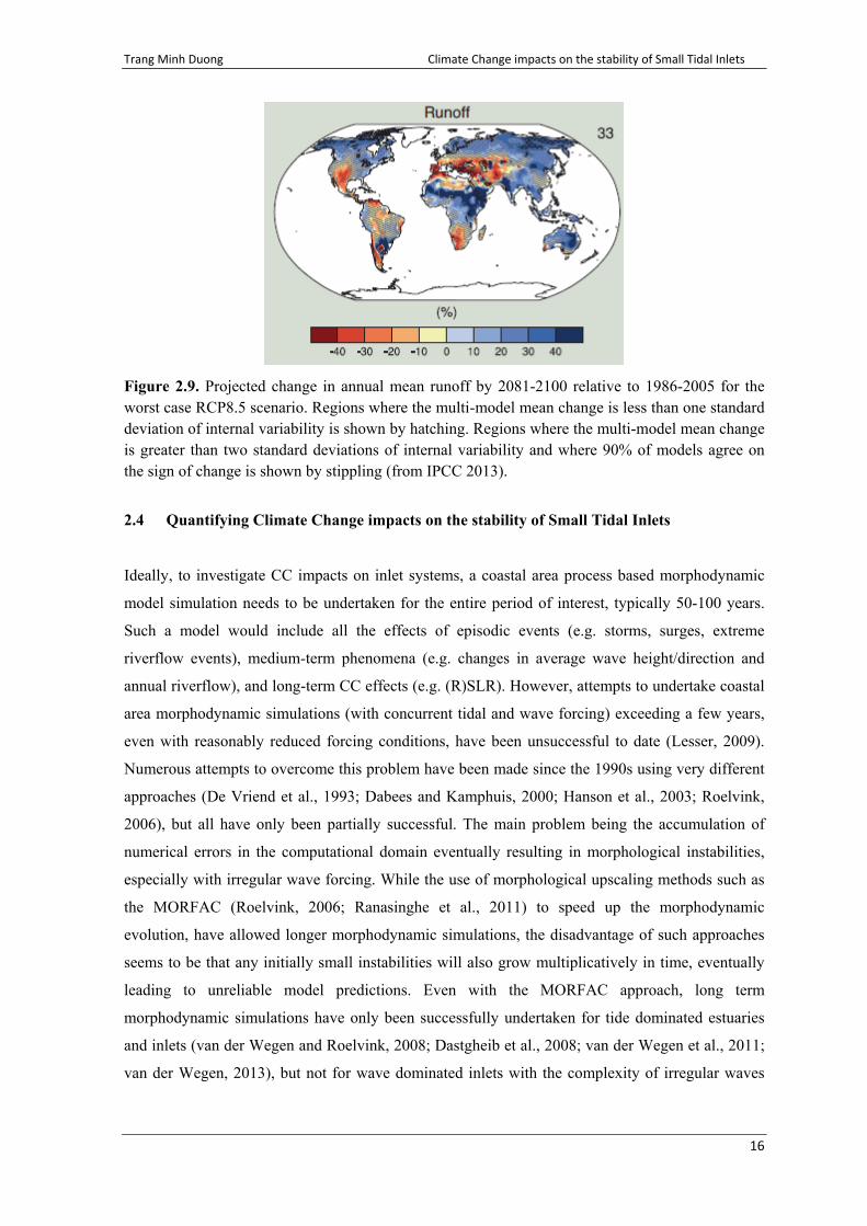
Figure 2.9. Projected change in annual mean runoff by 2081-2100 relative to 1986-2005 for the worst case RCP8.5 scenario. Regions where the multi-model mean change is less than one standard deviation of internal variability is shown by hatching. Regions where the multi-model mean change is greater than two standard deviations of internal variability and where 90% of models agree on the sign of change is shown by stippling (from IPCC 2013).
2.4 Quantifying Climate Change impacts on the stability of Small Tidal Inlets
Ideally, to investigate CC impacts on inlet systems, a coastal area process based morphodynamic
model simulation needs to be undertaken for the entire period of interest, typically 50-100 years.
Such a model would include all the effects of episodic events (e.g. storms, surges, extreme
riverflow events), medium-term phenomena (e.g. changes in average wave height/direction and
annual riverflow), and long-term CC effects (e.g. (R)SLR). However, attempts to undertake coastal
area morphodynamic simulations (with concurrent tidal and wave forcing) exceeding a few years,
even with reasonably reduced forcing conditions, have been unsuccessful to date (Lesser, 2009).
Numerous attempts to overcome this problem have been made since the 1990s using very different
approaches (De Vriend et al., 1993; Dabees and Kamphuis, 2000; Hanson et al., 2003; Roelvink,
2006), but all have only been partially successful. The main problem being the accumulation of
numerical errors in the computational domain eventually resulting in morphological instabilities,
especially with irregular wave forcing. While the use of morphological upscaling methods such as
the MORFAC (Roelvink, 2006; Ranasinghe et al., 2011) to speed up the morphodynamic
evolution, have allowed longer morphodynamic simulations, the disadvantage of such approaches
seems to be that any initially small instabilities will also grow multiplicatively in time, eventually
leading to unreliable model predictions. Even with the MORFAC approach, long term
morphodynamic simulations have only been successfully undertaken for tide dominated estuaries
and inlets (van der Wegen and Roelvink, 2008; Dastgheib et al., 2008; van der Wegen et al., 2011;
van der Wegen, 2013), but not for wave dominated inlets with the complexity of irregular waves

Trang Minh Duong Climate Change impacts on the stability of Small Tidal Inlets
17
(let alone seasonally changing riverflows). To date, morphodynamic simulations of wave-
dominated inlets that have resulted in realistic results have been limited in duration to a few months
(Ranasinghe et al., 1999; Bertin et al., 2009; Bruneau et al., 2011). Thus, a process based coastal
area (2DH) model that is capable of producing robust 50-100 year morphodynamic predictions
with concurrent water level, wave and riverflow forcing does not currently exist. Even if such a
model were available, the high computational demand of the model will not allow the multiple
simulations that would be required to adequately account for the large uncertainty stemming from
multiple sources (e.g. GHG scenarios, GCMs, morphodynamic model) that are inherent to CC
impact studies.
An alternative approach is to undertake strategic 'snap-shot' simulations using process based coastal
area models to gain some qualitative insights on how CC may affect inlet stability. In this
approach, a model that has been validated for present conditions can be applied with future forcing
for a simulation length of about 1 year at the desired future times (e.g. 2050, 2100) such that the
annual cycle of forcing and/or morphological behaviour is represented. This approach will provide
a good qualitative assessment of the potential impact of CC on inlet stability.
Snap-shot simulations to assess CC impacts on the stability of STIs may be designed and
implemented in two different ways depending on whether the application is in a "data rich" or "data
poor" environment. The basic rationale of both approaches is to 'validate' a 2DH morphodynamic
model to first reproduce the main observed contemporary system morphodynamic characteristics
(e.g. seasonal/intermittently closure; permanently open state; or alongshore migration) and then to
use the validated model to obtain projections of system behaviour under climate change forcing.
The two approaches are described below.
2.4.1 Data rich environments
A study area can be considered as 'data rich' when detailed bathymetries of the estuary, inlet and
nearshore zone (extending to about 20m depth); at least a few years of wave, wind and riverflow
data (ideally exceeding 10 years to encapsulate inter-annual variability); and downscaled future CC
modified wave and riverflow data are available for the desired planning horizon (e.g. 2100).
CC impact assessments invariably contain large uncertainties. A sequentially applied train of
numerical models could be used to account for these uncertainties. Ruessink and Ranasinghe
(2014) present an ensemble modelling framework (Figure 2.10) that could be used in a data rich
environment for robust assessment of CC impacts.

Trang Minh Duong Climate Change impacts on the stability of Small Tidal Inlets
18
Figure 2.10. Conceptual approach for the ensemble modelling of CC impacts on coasts at local scale (after Ruessink and Ranasinghe, 2014).
The approach starts from a global scale and zooms into a local site scale (~10 km length scale) via
a logical sequencing of Global Climate Models (GCMs), Regional Climate Models (RCMs),
GCM ensemble
GHG scenarios (SRES, RCP)
RCM ensemble
Regional/catchment scale coastal forcing models (waves, currents, riverflow)
Local scale coastal impact modes (e.g. DELFT3D, MIKE 21)
STEP 1: To account for scenario uncertainty
STEP 2: To account for GCM uncertainty
Dynamic downscaling
Bias correct for present time slice
STEP 3: To account for RCM uncertainty
STEP 4: Validate for present time slice and apply for future times to obtain projections to force coastal impact models with
STEP 5: Validate for present time slice and apply for future times to obtain full range of potential impacts

Trang Minh Duong Climate Change impacts on the stability of Small Tidal Inlets
19
Regional wave/hydrodynamic/catchment models, local wave models, and coastal impact models.
This ensemble modelling approach will provide a number of different projections of the coastal
impact under investigation. The range of projections will account for GHG scenario uncertainty,
GCM uncertainty, and RCM uncertainty. If necessary regional/catchment scale forcing model and
coastal impact model uncertainty can also be included in this approach at a significant computing
cost. The range of coastal impact projections thus obtained can then be statistically analysed to
obtain not only a best estimate of coastal impacts but also the range of uncertainty associated with
the projections, which will enable coastal managers/planners to make risk informed decisions.
In Step 5 of the above approach, a coastal impact model appropriate for investigating the desired
system diagnostic needs to be adopted. In the case considered herein, i.e. the stability of STIs, a
2DH morphodynamic model such as Delft3D or Mike21 may be used as described below (see also
Figure 2.11).
Hydrodynamic calibration/validation
As a necessary first step, the process based model should be calibrated/validated against
hydrodynamic measurements, such as water level and velocity, at several locations within the inlet-
estuary system. Ideally the model should be calibrated against data for at least one full spring-neap
cycle during both high and low riverflow conditions and subsequently validated for two spring-
neap cycles (both high and low riverflow conditions). To achieve a good model skill, it is crucial
that the grid size at the inlet channel and in the surf zone along the adjacent coast is sufficiently
fine to resolve physical processes occurring therein and that offshore and lateral domain boundaries
are sufficiently far from the inlet to prevent any boundary effects from propagating into the vicinity
of the inlet.
Morphodynamic validation
The hydrodynamically validated model may then be used to simulate the present morphodynamic
behaviour of the STI. The target of this 'present simulation' (PS) is to gain confidence in the
model's ability to simulate system morphodynamics by reproducing the general contemporary
morphodynamic behaviour of the system (e.g. closed/open, locationally stable/migrating).
Simulations should span at least one year to represent the annual cycle of riverflow (high/low
seasons) and wave conditions (winter/summer or monsoon/non-monsoon), or in the case of
seasonally/intermittently closing inlets, until inlet closure occurs. As the ensemble approach
recommended in Figure 2.10 will necessitate a substantial number of morphodynamic simulations,
undertaking all simulations with high resolution time series forcing will constitute an almost

Trang Minh Duong Climate Change impacts on the stability of Small Tidal Inlets
20
impracticable computational effort. Therefore, some level of temporal aggregation will be required.
In most cases, it will most likely be sufficient to use spring-neap cycle averaged riverflow and
wave conditions in a simulation of two full spring-neap cycles (~28 days) together with a
morphological acceleration (MORFAC) of 13 to allow the representation of approximately one
year of morphodynamics.
Figure 2.11. Schematic illustration of modelling approach for CC impacts assessment at STIs in data rich environments. Subscripts 'p' and 'f' refer to 'present' and 'future' respectively.
CC Impact Simulations
- SLR modified bathymetry
- Future forcing (SLR, waves, riverflow)
CC Input
- Downscaled projected wave climate (Hf, Tf, θf) (Step 4)
- Downscaled projected riverflow (Qf) (Step 4)
- Projected RSLR
Present Simulation
- Present bathymetry
- Present contemporary forcing input (tide, wave climate, riverflow)
- Quantitative hydrodynamic validation against measurements (velocity, water level)
- Qualitative validation with: empirical relationships, observed present system morphodynamic behavior and satellite images
Present Input
- Present time averaged average wave climate (Hp, Tp, θp)
- Present time averaged average riverflow (Qp)
Local scale coastal impacts model
(e.g. Delft3D, Mike21…)

Trang Minh Duong Climate Change impacts on the stability of Small Tidal Inlets
21
STI behaviour can strongly depend on the co-occurrence characteristics of riverflow and wave
conditions. For example, when high energy (or highly obliquely incident) waves (i.e. large
longshore sediment transport - LST) co-exist with high riverflow (i.e. high ebb flow velocities
through inlet), the hydraulic capacity to flush out the sediment deposited in the inlet mouth will be
high, and therefore the inlet will remain stable. On the other hand, when riverflow is low (with the
same wave conditions), the ebb flow velocities will be lower, and therefore the hydraulic capacity
to flush out sand deposited in the inlet mouth will be much reduced, potentially leading to inlet
closure or migration. Thus, it is important that any input reductions made to increase computational
efficiency do not affect concurrent temporal variations in forcing that exist in nature.
Model results may be compared with empirical relationships such as the A-P relationship, Escoffier
curve, and Bruun inlet stability criteria. Furthermore, model results may also be qualitatively
validated using any available aerial/satellite images of the study areas.
Climate Change impact projections
The validated model may now be applied to investigate CC impacts on the STI. The CC impact
simulations should account for the full range of potential CC driven variations in system forcing
(mean water level, waves, riverflow). The future projected RSLR (accounting also for regional
effects on sea level) may be calculated using the approach prescribed by Nicholls et al. (2014),
while CC modified future wave climate and riverflow can be obtained from the dynamically
downscaled, regional output from Regional/catchment scale coastal model, after Step 4 in the
Ensemble modelling approach shown in Figure 2.10.
The CC impact snap-shot simulations may also be undertaken for the same duration as the PS
(unless in the case of Seasonally/Intermittently open inlets, in which the simulation needs to
continue only until inlet closure occurs). An important long term process that needs to be (and can
be) accounted for in these simulations is SLR driven basin infilling. This process occurs due to the
increase in estuary/lagoon (or basin) volume below mean water level as a result of SLR (i.e.
'accommodation space'). As the basin strives to maintain an equilibrium volume, it will import
sediment from offshore to raise the basin bed level such that the pre-SLR basin volume is
maintained. Depending on sediment availability, when a sand volume equal to the SLR induced
accommodation space (SLR x surface area of basin) is imported into the basin, the basin will reach
equilibrium. Stive et al. (1998), however point out that in most situations there will be a lag
between the rate of SLR and basin infilling due to the time scale disparity between hydrodynamic
forcing and morphological response. Using volume balance considerations, Ranasinghe et al.
(2013) have shown that for STIs, this lag could be about 0.5 over the 21st century (i.e. the basin

Trang Minh Duong Climate Change impacts on the stability of Small Tidal Inlets
22
infill volume by the end of the 21st century is equal to half of the SLR driven increase in
accommodation space over the same period). Using these approximations, the long term process of
basin infilling can be accommodated in snap-shot simulations by adjusting the initial bathymetry of
the future simulations. Attention should be paid however to ensure that the adjusted future
bathymetry maintains the contemporary basin hypsometry (Boon and Byrne, 1981).
A series of CC impact snap-shot simulations, where individual CC modified forcings are
sequentially excluded from an initial all-inclusive simulation (e.g. SLR + CC Waves + CC
Riverflow; SLR + CC Waves; SLR + CC Riverflow; and SLR only) should ideally be undertaken
to investigate the relative contribution of the various CC modified forcings to potential changes in
inlet stability.
2.4.2 Data poor environments
At most locations however, especially in developing countries, the data required for the approach
described in Section 2.4.1 is not available. Especially, good bathymetry data and future downscaled
forcing from sophisticated and computationally expensive Regional Scale modelling (Step 3 in
Figure 2.10) approach are very unlikely to be available at most locations. In such data poor
environments, a strategic schematized modelling approach may be used as described below to
obtain a 'first-pass-assessment' of CC impacts on STIs (see also Figure 2.12). This approach does
however assume the availability of at least good guestimates of contemporary monthly averaged
riverflows and wave conditions.
Schematized bathymetry
In this approach, a simplified schematized bathymetry can be used to qualitatively represent the
real system bathymetry. Over the last decade, this approach has been successfully used to gain
qualitative insights into inlet morphodynamics of diverse inlet-estuary/lagoon systems at various
time scales (Marciano et al., 2005; Dastgheib et al., 2008; van der Wegen and Roelvink, 2008; van
der Wegen et al., 2010; Nahon et al., 2012; Dissanayake et al., 2012; van Maanen et al., 2013;
Zhou et al., 2014).

Trang Minh Duong Climate Change impacts on the stability of Small Tidal Inlets
23
Figure 2.12. Schematic illustration of modelling approach for CC impact assessment at STIs in data poor environments. Subscripts 'p' and 'f' refer to 'present' and 'future' respectively.
Following the philosophy adopted in these previous studies, an STI system schematized
bathymetry could consist of a rectangular estuary/lagoon of constant depth connected to the ocean
via a straight, constant depth channel. The dimensions of the schematized system (estuary/lagoon
and inlet channel width/length) should be chosen such that they closely represent a real-life system,
based on for e.g. Google Earth images. The mean depth of the estuary/inlet channel may be gleaned
from any available literature, from local expert judgment or one-off, low-tech spot measurements.
CC Impact Simulations
- SLR modified bathymetry
- Future forcing (SLR, waves, riverflow), account for all possible combinations of CC modified forcing
CC Input
- Published projected changed wave climate (Hf, Tf, θf) (Hemer et al., 2013)
- Published projected riverflow (Qf) (IPCC, 2013)
- Projected SLR (IPCC, 2013)
Present Simulation
- Schematized initial bathymetry
- Present contemporary forcing input (tide, wave climate, riverflow)
- Qualitative validation with: empirical relationships, observed present system morphodynamic behavior and satellite images (if available)
Present Input
- Present monthly average wave climate (Hp, Tp, θp)
- Present monthly average riverflow (Qp)
Local scale coastal impacts model
(e.g. Delft3D, Mike21…)

Trang Minh Duong Climate Change impacts on the stability of Small Tidal Inlets
24
The bathymetry of the ocean side could consist of shore-parallel depth contours such that a Dean’s
equilibrium profile (with D50 depending on local conditions) is followed up to about 10-20m depth.
Riverflow may be introduced into the estuary/lagoon at roughly the same location the main
riverflow enters the system based on Google Earth or Satellite images. Care should be taken to
ensure that the grid size at the small inlet mouth and in the surf zone along the adjacent coast is fine
enough to adequately resolve the physical processes occurring therein. Figure 2.13 shows an
example initial bathymetry of such a schematized STI system.
Figure 2.13. Example of schematized bathymetry for Maha Oya Inlet (Right) with: inlet width = 100m, inlet length = 70 m, inlet depth = 3 m; estuary width = 200 m, estuary length = 1000 m, estuary depth = 3.5 m; river width = 100 m, nearshore bed slope follows Dean equilibrium profile for D50 of 0.25 mm. Satellite image (left) from Google Earth.
CC modified forcing
To circumnavigate the typical unavailability of downscaled future forcing in data poor
environments, future forcing needs to be sourced from the freely available sources described in
Section 2.3 above. Future SLR may be obtained from Table 2.2 and Figure 2.5 while future
riverflows may be obtained from Figure 2.9 for the worst case IPCC scenario. Future wave forcing
may be obtained from the ensemble global downscaling results presented by Hemer et al. (2013)
(reproduced above in Figs 2.6-2.8). It should be borne in mind that these freely available global
scale future projections, particularly of riverflow and waves, are at a much coarser resolution than
that would be produced by a site-specific downscaling study (as in data rich environments).
Therefore, the aforementioned global maps of projected change will only give approximate
indications of how these system forcings might change (e.g. as area averaged % increase/decrease
relative to the present).These changes then need to be superimposed on available contemporary
riverflow/wave data to derive future forcing conditions for the coastal impact model.

Trang Minh Duong Climate Change impacts on the stability of Small Tidal Inlets
25
Morphodynamic validation
As in the case of data rich environments, a Present simulation (PS) should be undertaken to at least
qualitatively validate the model against observed present behaviour of the STI. The model,
initialised with the above described schematized bathymetry can be forced with schematized
harmonic tidal forcing (say, an M2 harmonic with approximate observed mean tidal amplitude in
the study area) and monthly averaged time series of waves and of riverflow.
In this case too, the PS should span at least one year to represent the annual cycles of riverflow and
wave conditions, or in the case of seasonally/intermittently closing inlets, until inlet closure occurs.
Due to the monthly averaged forcing, it is sufficient here to use a MORFAC of 30, such that one
day of the hydrodynamic simulation will represent a month (30 days) of morphodynamics. Model
results can be qualitatively validated following the same approach described for PS validation in
data rich environments (i.e. using empirical relationships and aerial/satellite imagery).
Climate Change impact projections
The qualitatively validated model may then be forced with CC modified forcing conditions
(derived as described above), following the same approach outlined for data rich environments.
Due to the flat bed of the initial bathymetry, here, the basin infilling effect may simply be
represented by raising the estuary/lagoon bed level by approximately half the SLR amount
following the argumentation presented by Ranasinghe et al. (2013).
While this approach will provide a useful first-pass assessment of CC impacts on the stability of
STIs in data poor environments, the uncertainty associated with the projections will be high due to
the coarse and approximate model forcing and schematisation of system bathymetry. Therefore, if
this approach indicates any signs of future inlet stability being significantly different from the
present situation, it would be prudent to undertake a more detailed study (including targeted data
collection and GCM downscaling).
2.5 Discussion
While the snap-shot simulation approach described above will provide insights on inlet stability
that are useful for coastal zone management/planning, it also has several shortcomings. One of the
major shortcomings is that this approach will not be able to take into account slow gradual
morphological changes (excepting the SLR driven basin infilling process) that may occur from
'present' to 'future'. For example, any gradual CC driven changes in average wave direction could

Trang Minh Duong Climate Change impacts on the stability of Small Tidal Inlets
26
change the orientation of the coastline along which the target STI is located. This may have
implications on the future longshore sediment transport rate and inlet dimensions (and therefore
tidal prism), thus affecting inlet stability. Slow changes in longshore sediment transport rate and
riverflow may also in some cases result in the development of extensive flood shoals in the lower
reaches of the estuary/lagoon (close to the inlet channel) which could affect tidal attenuation, and
hence the tidal prism, thus influencing inlet stability. Furthermore, the above snap-shot modelling
approach will not account for any irreversible morphological changes that may be caused by CC
modified extreme storm surge events (e.g. breaching of new inlets) and riverflows (e.g. ebb/flood
delta development).
To obtain reliable projections of CC impacts on the stability of STIs, what is ideally required is a
multi-scale coastal impact model that can accurately simulate the various physical processes
occurring at different spatio-temporal scales. Such a model should incorporate both cross-shore
(vertically non-uniform) and longshore (more or less vertically uniform) hydrodynamics to
simulate coastal hydrodynamics relevant for episodic, medium-term, and long-term STI
morpodynamics. Thus, the model needs to be a coastal area model with at least quasi 3D if not
fully 3D hydrodynamics. To avoid the inevitable far field instabilities that will creep into the area
of interest when using a gridded approach for morphodynamics, some spatio-temporal aggregation
of hydrodyamics prior to calculating bed level changes may be required. However, as such a new
multi-scale modelling approach might take years (or decades) to develop, an interim solution may
be found in scale aggregated (or reduced complexity) models. This type of models, if correctly
developed, may be used to obtain the full temporal evolution of CC driven variations in STI
stability. In such a scale aggregated model, following the rationale presented by Stive and Wang
(2003) and Ranasinghe et al. (2013), the main physical processes governing the main diagnostic (in
this case: inlet stability) may be parameterised and collectively represented by a fully explicit
governing equation. This would result in a very fast model that enables the multiple simulations
required to quantify the uncertainties associated with assessing CC impacts on STI stability.
2.6 Summary and Conclusions
Climate change driven variations in mean water level (i.e. SLR), wave conditions and riverflow are
likely to affect the stability of the thousands of Small tidal Inlets (STIs, or bar-built/barrier estuary
systems) around the world. Due to their pre-dominant occurrence in tropical and sub-tropical
zones, this type of inlets are commonly found in developing countries, where data availability is
generally sub-optimal (i.e. data poor environments) and community resilience to coastal changes is
low. Furthermore, STI environs in developing countries especially host a number of economic

Trang Minh Duong Climate Change impacts on the stability of Small Tidal Inlets
27
activities (and thousands of associated livelihoods) such as harbouring sea going fishing vessels,
inland fisheries (e.g. prawn farming), tourist hotels and tourism associated recreational activities
which contribute significantly to the national GDPs. This combination of pre-dominant occurrence
in developing countries, socio-economic relevance and low community resilience, general lack of
data, and high sensitivity to seasonal forcing makes STIs potentially very vulnerable to CC
impacts.
This Chapter provides a summary description of how CC may affect the stability of STIs and how
these CC impacts maybe quantified using existing modelling tools. Due to the unavailability of
process based models that can be confidently applied with concurrent time varying water level,
wave and riverflow forcing over typical CC impact assessment time scales (~100 years), 'snap-shot'
simulations (~1 year duration) of process based coastal area morphodyamic models are proposed as
a means of obtaining qualitative assessments of CC impacts on STIs. Two different 'snap-shot'
modelling frameworks for data rich and data poor environments are presented. The main
shortcomings of the proposed 'snap-shot' modelling approach are identified as non-consideration of
CC driven slow gradual morphological changes (except SLR driven basin infilling) and irreversible
morphological changes due to CC modified extreme storm surge, wave, riverflow events. To obtain
more reliable assessment of CC impacts on STIs, the development of process based multi-scale
coastal area morphodynamic models and scale aggregated morphodynamic models are identified as
future research needs.
References
Bertin, X., Fortunato, A.B., Oliveira, A., 2009. A modeling-based analysis of processes driving wave-dominated inlets. Continental Shelf Research, 29 (5-6), 819-834.
Boon, J.D., Byrne, R.J., 1981. On basin hypsometry and the morphodynamic response of coastal inlet systems. Marine Geology, 40, 27-48.
Bruneau, N., Fortunato, A.B., Dodet, G., Freire, P., Oliveira, A., Bertin, X., 2011. Future evolution of a tidal inlet due to changes in wave climate, sea level and lagoon morphology: O´bidos lagoon, Portugal. Continental Shelf Research 31, 1915-1930.
Bruun, P., 1978. Stability of tidal inlets – theory and engineering. Developments in Geotechnical Engineering. Elsevier Scientific, Amsterdam, 510p.
Bruun, P., Gerritsen, F., 1960. Stability of coastal inlets. North-Holland Publishing Co., Amsterdam, 123p.
Carter, R. W. G. and Woodroffe, C. D., 1994. Coastal evolution: Late quaternary shoreline morphodynamics. Cambridge university press, 517p.

Trang Minh Duong Climate Change impacts on the stability of Small Tidal Inlets
28
Dabees, M., Kamphuis, J.W., 2000. ONELINE: Efficient Modeling of 3D Beach Change. 2000. Proceedings of the 27th International Conference on Coastal Engineering, Sydney, Australia, ASCE, pp. 2700-2713.
Dastgheib, A., Roelvink, J.A., Wang, Z.B., 2008. Long-term process-based morphological modeling of the Marsdiep Tidal Basin. Marine Geology, 256 (1-4), 90-100.
Davis, R.A., FitzGerald, D.M., 2004. Beaches and coasts. Blackwell Publishing. 419p.
DeVriend, H.J., Zyserman, J., Nicholson, J., Roelvink. J.A., Pechon, P., Southgate, H.N., 1993. Medium term 2DH coastal area modelling. Coastal Engineering, 21, 193-224.
Dissanayake P. K.., Ranasinghe, R., Roelvink, D., 2012. The morphological response of large tidal inlet/basin systems to sea level rise. Climatic Change, 113, 253-276.
Escoffier, F.F., 1940. The stability of tidal inlets. Shore and Beach, 8,111-114.
FitzGerald, D.M., 1988. Shoreline erosional-depositional processes associated with tidal inlets. In: Lecture Notes on Coastal and Estuarine Studies, Vol.129, Hydrodynamics and Sediment Dynamics of Tidal Inlets (Eds. Aubrey, D.G., Weishar, L.), Springer-Verlag, pp. 186-225.
FitzGerald, D.M., Fenster, M.S., Argow, B.A., Buynevich, I.V., 2008. Coastal impacts due to sea-level rise. Annual Review of Earth and Planetary Sciences, 36, 601-647.
Hanson, H., Aarninkhof, S., Capobianco, M., Jimenez, J.A., Larson, M., Nicholls, R., Plant, N., Southgate, H.N., Steetzel, H.J., Stive, M.J.F., De Vriend, H.J., 2003. Modelling coastal evolution on early to decadal time scales. Journal of Coastal Research, 19(4), 790-811.
Hemer, M., Fan, Y., Mori, N., Semedo, A., Wang, X.L., 2013. Projected changes in wave climate from a multi-model ensemble. Nature Climate Change, 3, 471-476.
IPCC, 2013. Summary for Policymakers. In: Climate Change 2013: The Physical Science Basis. Contribution of Working Group I to the Fifth Assessment Report of the Intergovernmental Panel on Climate Change [Stocker, T.F., D. Qin, G.-K. Plattner, M. Tignor, S.K. Allen, J. Boschung, A. Nauels, Y. Xia, V. Bex and P.M. Midgley (eds.)]. Cambridge University Press, Cambridge, United Kingdom and New York, NY, USA.
Jarrett, J.T., 1976. Tidal prism – inlet area relationships. Technical Report GITI No.3, CERC, U.S. Army Engineer Waterways Experiment Station, Vicksburg, MS.
Lesser, G., 2009. An approach to medium-term coastal morphological modeling. PhD thesis. UNESCO-IHE/Delft University of Technology, ISBN 978-0-415-55668-2.
Marciano, R., Wang, Z.B., Hibma, A., de Vriend, H.J., Defina, A., 2005. Modeling of channel patterns in short tidal basins. Journal of Geophysical Research, 110, F01001, doi: 10.1029/2003JF000092.
Nahon, A., Bertin, X., Fortunato, A.B., Oliveira, A., 2012. Process-based 2DH morphodynamic modeling of tidal inlets: A comparison with empirical classifications and theories. Marine Geology, 291–294, 1–11, doi:10.1016/j.margeo.2011.10.001.
Nicholls, R.J., Hanson, S., Lowe, J.A., Warrick, R.A., Lu, X., Long, A.J., 2014. Sea-level scenarios for evaluating coastal impacts. Wiley Interdisciplinary Reviews: Climate Change 5 (1), 129-150.

Trang Minh Duong Climate Change impacts on the stability of Small Tidal Inlets
29
O’Brien, M.P., 1931. Estuary and tidal prisms related to entrance areas. Civil Engineering 1(8), 738-739.
O’Brien, M.P., 1969. Equilibrium flow areas of inlets on sandy coasts. Journal of Waterways and Harbour Division, 95, 43-52.
Ranasinghe, R., Pattiaratchi, C., Masselink, G., 1999. A morphodynamic model to simulate the seasonal closure of tidal inlets. Coastal Engineering, 37(1), 1-36.
Ranasinghe, R., Swinkels, C., Luijendijk, A., Roelvink, D., Bosboom, J., Stive, M., Walstra, D., 2011. Morphodynamic upscaling with the MORFAC approach: Dependencies and sensitivities. Coastal Engineering, 58, 806-811.
Ranasinghe, R., Duong, T.M., Uhlenbrook, S., Roelvink, D., Stive, M., 2013. Climate change impact assessment for inlet-interrupted coastlines. Nature Climate Change, 3, 83-87, DOI.10.1038/NCLIMATE1664.
Ruessink, B.G., Ranasinghe, R., 2014. Beaches. In: Coastal Environments and Global Change (Eds. Masselink, G. and Gehrels, R.). Wiley, pp. 149-176.
Roelvink, J.A., 2006. Coastal morphodynamic evolution techniques. Coastal Engineering, 53, 277-287.
Small, C., Nicholls, R.J., 2003. A global analysis of human settlement in coastal zones. Journal of Coastal Research, 19(3), 584-599.
Stive, M. J. F., Capobianco, M., Wang, Z. B., Ruol, P., Buijsman, M. C., 1998. Morphodynamics of a tidal lagoon and the adjacent coast. Proceedings of the Eighth International Biennial Conference on Physics of Estuaries and Coastal Seas, The Hague, pp.397- 407.
Stive, M.J.F., Wang, Z.B., 2003. Morphodynamic modelling of tidal basins and coastal inlets. Advances in Coastal Modelling (Ed. C. Lakhan). Elsevier Science B.V, pp. 367-392.
van der Wegen, M., 2013. Numerical modeling of the impact of sea level rise on tidal basin morphodynamics, Journal of Geophysical Research, 118, doi:10.1002/jgrf.20034.
van der Wegen, M., Jaffe, B. E., Roelvink, J. A., 2011. Process-based, morphodynamic hindcast of decadal deposition patterns in San Pablo Bay, California, 1856-1887, Journal of Geophysical Research, 116, F02008, doi: 10.1029/2009JF001614.
van der Wegen, M., Roelvink, J.A., 2008. Long-term morphodynamic evolution of a tidal embayment using a two-dimensional, process-based model. Journal of Geophysical Research., 113, C03016, doi: 10.1029/2006JC003983.
van der Wegen, M., Dastgheib, A., Roelvink, J.A., 2010. Morphodynamic modeling of tidal channel evolution in comparison to empirical PA relationship. Coastal Engineering. 57, 827-837, doi:10.1016/j.coastaleng.2010.04.003.
van Maanen, B., Coco, G., Bryan, K.R., Friedrichs, C.T., 2013b. Modeling the morphodynamic response of tidal embayments to sea-level rise. Ocean Dynamics, 63(11-12), 1249-1262, doi:10.1007/s10236-013-0649-6.
Zhou, Z, Coco, G., Jiminez, M., Olabarrieta, M, van der Wegen, M, Townend, I. 2014. Morphodynamics of river influenced back barrier tidal basins: The role of landsacpe and hydrodynamic settings, Water Resources Research, 50, doi: 10.1002/2014WR015891.

Trang Minh Duong Climate Change impacts on the stability of Small Tidal Inlets
30
CHAPTER 3
ASSESSING CLIMATE CHANGE IMPACTS ON THE STABILITY OF SMALL TIDAL INLETS IN DATA POOR ENVIRONMENTS
3.1 Introduction
This Chapter demonstrates the application of the process based snap-shot modelling approach for
data poor environments proposed in Section 2.4.2 of Chapter 2. The approach is applied to 3 case
study sites representing the 3 main STI types described above: Negombo lagoon (Type 1); Kalutara
lagoon (Type 2); and Maha Oya river (Type 3); all of which are located along the SW coast of Sri
Lanka (Figure 3.1).
3.2 Methodology
3.2.1 Study areas
Sri Lanka, is an island nation of about 65,610 km2 area located in the Indian Ocean, Southeast of
India (Figure 3.1). The country has a tropical monsoon climate, with 2 monsoon seasons; the
Northeast (NE) monsoon from November-February and the Southwest (SW) monsoon from May-
September. About one third of the total annual rainfall occurs between October and December
(Zubair and Chandimala, 2006). The coastal environment of Sri Lanka is wave dominated (average
offshore significant wave height of 1.12m) and micro-tidal (mean tidal range of approximately
0.5m). The SW coast of Sri Lanka generally experiences the most energetic wave conditions during
the SW monsoon when offshore significant wave heights are between 1 and 2 m and mean wave
direction is from the SW-W octant. The beaches around the country are composed of quartz sand
with grain diameters (D50) varying between 0.2-0.45mm.

Trang Minh Duong Climate Change impacts on the stability of Small Tidal Inlets
31
Figure 3.1. Location of Sri Lanka (left) and the 3 case study sites (right). Source: Google Earth.
Negombo lagoon
Negombo lagoon is located about 30 km North of Colombo (Figure 3.2, left) and is connected to
the ocean via a permanently open, relatively wide (400 m), short (300 m) and shallow (3 m) inlet
which is locationally stable. The lagoon has a surface area of around 45 km2 and the average depth
is approximately 1 m. The net annual longshore sediment transport rate in the vicinity of the inlet is
insignificant (Chandramohan et al., 1990). This is due to the sheltering effect provided by the
offshore reef to the west of the inlet (Figure 3.2, left). The sediment on the coast adjacent to the
inlet has a D50 of 0.25 mm (University of Moratuwa, 2003). The majority of the catchment of the
Negombo lagoon is located in the SW of the country and therefore most of the riverflow into the
lagoon occurs during the SW monsoon. Dandugam Oya, Ja Ela and several streams from
Muthurajawela flow into the lagoon with a combined average annual riverflow volume that varies
from almost 0 m3/s during dry seasons to more than 200 m3/s during rainy seasons (University of
Moratuwa, 2003)).
Figure 3.2. Negombo lagoon (left), Kalutara lagoon (middle), Maha Oya river (right) (Source: Google Earth).
Galle
Puttalam

Trang Minh Duong Climate Change impacts on the stability of Small Tidal Inlets
32
Kalutara Lagoon
Kalutara lagoon is located about 40 km South of Colombo (Figure 3.2, middle). The Kalu River,
with the second highest annual riverflow volume (7500 million m3/yr) in the country, discharges
into the ocean via this lagoon. The lagoon is connected to the ocean via a permanently open,
alongshore migrating inlet with average width 150 m, length 150 m and depth 4.5m. Historically,
the longshore migration of the Kalutara lagoon inlet comprised a 3-4 year cycle during which the
inlet migrated about 2 km to the south (~500m/yr southerly migration) before a new, more
hydraulically efficient inlet was either naturally or artificially created at the northern end of the
lagoon barrier (Perera, 1993). The lagoon has a surface area of only around 2 km2 and the average
depth is approximately 3 m. The net longshore sediment transport rate in the area is about 0.5
million m3/yr to the south (GTZ, 1994). The sediment on the coast adjacent to the inlet has a D50 of
0.25 mm. The catchment of the Kalu river is the 2nd largest in the country (2766 km2) and it
receives rainfall from both the SW and NE monsoons, resulting in river discharges that are
consistently higher than 100 m3/s throughout the year (with peaks exceeding 300 m3/s in May and
October). The average river discharge of the Kalu river is 250 m3/s.
Maha Oya River
Maha Oya inlet (Figure 3.2, right), through which the Maha Oya river discharges (1571 million
m3/yr) into the ocean, is located about 40 km North of Colombo. The inlet, which is about 100 m
wide, 70 m long and 3 m deep, closes whenever the riverflow is small, regardless of the prevailing
longshore sediment transport regime. The lagoon surface area is about 0.2 km2 with an average
depth of 3-4 m. The net longshore sediment transport rate in the vicinity of the inlet is about
500,000m3/year to the North (GTZ, 1994). The sediment on the coast adjacent to the inlet has a D50
of 0.25 mm. The 1528 km2 catchment of Maha Oya derives most of its riverflow during the NE
monsoon. The average river discharge is about 50 m3/s with a peak of ~140 m3/s in November.
3.2.2 Schematized bathymetries
Schematized flat bed bathymetries were created for the 3 systems based on site descriptions in
published literature, Google Earth images and input from local experts. The key system dimensions
thus gleaned and used in creating the schematized bathymetries (Figure 3.3) are shown in Table
3.1. The nearshore zone was configured such that it consisted shore parallel depth contours that
follow a Dean's equilibrium profile in the cross-shore direction corresponding with the reported D50
for the area (also given in Table 3.1) down to 10m depth. Model grids for the 3 systems were
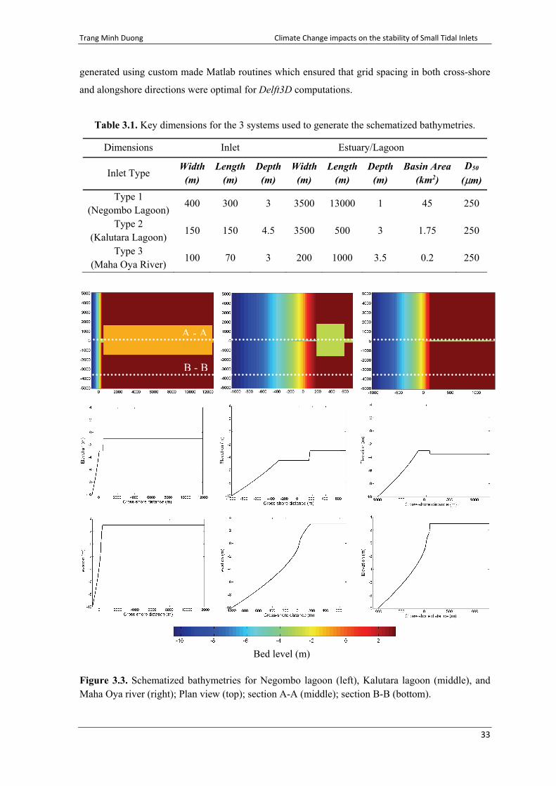
Trang Minh Duong Climate Change impacts on the stability of Small Tidal Inlets
33
generated using custom made Matlab routines which ensured that grid spacing in both cross-shore
and alongshore directions were optimal for Delft3D computations.
Table 3.1. Key dimensions for the 3 systems used to generate the schematized bathymetries.
Dimensions Inlet Estuary/Lagoon
Inlet Type Width
(m) Length
(m) Depth
(m) Width
(m) Length
(m) Depth
(m) Basin Area
(km2) D50
(μm)
Type 1 (Negombo Lagoon)
400 300 3 3500 13000 1 45 250
Type 2 (Kalutara Lagoon)
150 150 4.5 3500 500 3 1.75 250
Type 3 (Maha Oya River)
100 70 3 200 1000 3.5 0.2 250
Figure 3.3. Schematized bathymetries for Negombo lagoon (left), Kalutara lagoon (middle), and Maha Oya river (right); Plan view (top); section A-A (middle); section B-B (bottom).
A - A
B - B
Bed level (m)

Trang Minh Duong Climate Change impacts on the stability of Small Tidal Inlets
34
3.2.3 Schematized forcing
The mean ocean tidal range for all 3 systems (which are located along a single coastal stretch not
exceeding 100km) was taken as 0.5m based on published values (Wijeratne, 2002; University of
Moratuwa, 2003). Time series of monthly averaged riverflow were constructed for the 3 systems
(Figure 3.4) based on available sparse data and local publications. Wave conditions at 10 m depth
for each case study site (Figure 3.5) were extracted from regional SWAN model extending from
Galle to Puttalam along the SW coast (wave directions shown have been adjusted to account for the
differences between the coastline orientations at the study sites and the N-S coastline orientations
adopted in the schematized bathymetries). Comparison of hourly and monthly averaged conditions
at Colombo showed that monthly averaged values do not significantly under or over represent
actual wave conditions. Note that while most of the waves are < 2700 at Maha Oya (with respect to
the coordinate system adopted in the schematized bathymetries), all waves are > 2700 at Kalutara.
This is due to wave refraction over a large canyon located slightly north of Kalutara. At Negombo,
waves are more or less shore normal at 10 m depth. This is because all waves from the SW sector
(pre-dominant offshore wave direction) are completely diffracted by an offshore low crested (and
in places emergent) reef and subsequently sharply refracted to the nearshore to result in almost
shore normal nearshore waves throughout the year.
Figure 3.4. Riverflow forcing conditions for Negombo lagoon (left), Kalutara lagoon (middle), and Maha Oya river (right).

Trang Minh Duong Climate Change impacts on the stability of Small Tidal Inlets
35
Figure 3.5. Wave forcing conditions for Negombo lagoon (left), Kalutara lagoon (middle) and Maha Oya river (right); Top: Significant wave height, Bottom: Mean wave direction.
3.2.4 Process based model
The process based model Delft3D was extensively used in this study. Delft3D seamlessly combines
a short wave driver (SWAN), a 2DH flow module, a sediment transport model (Van Rijn, 1993),
and a bed level update scheme that solves the 2D sediment continuity equation. To accelerate
morphodynamic computations, Delft3D adopts the MORFAC approach (Roelvink, 2006;
Ranasinghe et al., 2011). This approach exploits the fact that time scales associated with bed level
changes are generally much greater than those associated with hydrodynamic forcing by essentially
multiplying the bed levels computed after each hydrodynamic time step by a time varying or
constant factor (MORFAC) to enable much faster computation. The significantly upscaled new
bathymetry is then used in the next hydrodynamic step. The model is fully described by Lesser et
al. (2004) and is therefore not described any further here. The basic model structure is shown in
Figure 3.6.

Trang Minh Duong Climate Change impacts on the stability of Small Tidal Inlets
36
Figure 3.6. Delft3D Model structure. To avoid boundary instabilities affecting the area of interest (i.e. the inlet entrance), the flow
computational domains were constructed such that they extended 5 km either side of the inlet for
all 3 study areas (Figure 3.7). Wave domains were created larger than flow domains to avoid any
wave shadowing effect at lateral boundaries.
Figure 3.7. Delft3D flow (inside the white dashed box) and wave domains used for the Kalutara lagoon case study (Type 2 inlet).
Initial bed
Tidal
Next time step
HydrodynamicsBoundaryconditions
Morphologicalscale factor
Sedimenttransport
Bed levelupdate
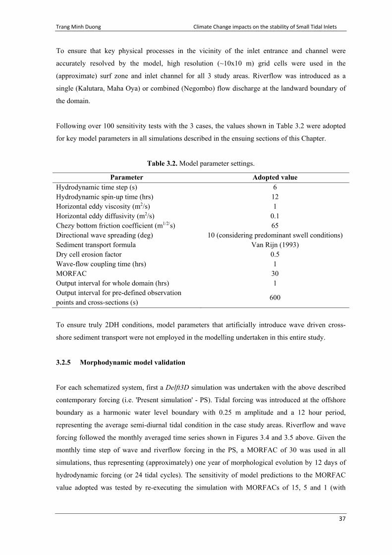
Trang Minh Duong Climate Change impacts on the stability of Small Tidal Inlets
37
To ensure that key physical processes in the vicinity of the inlet entrance and channel were
accurately resolved by the model, high resolution (~10x10 m) grid cells were used in the
(approximate) surf zone and inlet channel for all 3 study areas. Riverflow was introduced as a
single (Kalutara, Maha Oya) or combined (Negombo) flow discharge at the landward boundary of
the domain.
Following over 100 sensitivity tests with the 3 cases, the values shown in Table 3.2 were adopted
for key model parameters in all simulations described in the ensuing sections of this Chapter.
Table 3.2. Model parameter settings.
Parameter Adopted value Hydrodynamic time step (s) 6 Hydrodynamic spin-up time (hrs) 12 Horizontal eddy viscosity (m2/s) 1 Horizontal eddy diffusivity (m2/s) 0.1 Chezy bottom friction coefficient (m1/2/s) 65 Directional wave spreading (deg) 10 (considering predominant swell conditions) Sediment transport formula Van Rijn (1993) Dry cell erosion factor 0.5 Wave-flow coupling time (hrs) 1 MORFAC 30 Output interval for whole domain (hrs) 1 Output interval for pre-defined observation points and cross-sections (s)
600
To ensure truly 2DH conditions, model parameters that artificially introduce wave driven cross-
shore sediment transport were not employed in the modelling undertaken in this entire study.
3.2.5 Morphodynamic model validation
For each schematized system, first a Delft3D simulation was undertaken with the above described
contemporary forcing (i.e. 'Present simulation' - PS). Tidal forcing was introduced at the offshore
boundary as a harmonic water level boundary with 0.25 m amplitude and a 12 hour period,
representing the average semi-diurnal tidal condition in the case study areas. Riverflow and wave
forcing followed the monthly averaged time series shown in Figures 3.4 and 3.5 above. Given the
monthly time step of wave and riverflow forcing in the PS, a MORFAC of 30 was used in all
simulations, thus representing (approximately) one year of morphological evolution by 12 days of
hydrodynamic forcing (or 24 tidal cycles). The sensitivity of model predictions to the MORFAC
value adopted was tested by re-executing the simulation with MORFACs of 15, 5 and 1 (with

Trang Minh Duong Climate Change impacts on the stability of Small Tidal Inlets
38
appropriate changes in the forcing time series and wave-flow coupling time). Only marginal
differences were observed among the morphodynamic predictions of the test simulations,
indicating a MORFAC of 30 could be confidently used for the simulations presented herein.
Validation simulations for Type 1 and Type 2 systems were undertaken for one year to represent
the annual cycle of riverflow (high/low seasons) and wave conditions (monsoon/non-monsoon
periods) while the Type 3 system simulation was continued only until inlet closure occurred.
The target of this PS is to gain confidence in the model's ability to simulate system
morphodynamics by reproducing the general contemporary morphodynamic behaviour (e.g.
close/open, and locationally stable/migrating) of the system. To this end, model results were first
qualitatively validated using available aerial/satellite images of the study areas by comparing the
general observed and modelled morphodynamic behaviour of the systems. Secondly, model results
were compared against several empirical relationships such as the A-P relationship (O'Brien, 1931;
Jarrett 1976), Escoffier curve, and Bruun inlet stability criteria where possible. For these
comparisons, it is necessary to extract information regarding inlet cross-section area (A), the tidal
prism (P), maximum inlet current velocity (Vmax), and annual longshore sediment transport rates
(M). In the case studies selected here, riverflow is non-trivial, and therefore enhances the ebb tidal
prism (due to the tide effect only) which is one of the two processes that govern the main
diagnostic of this study, inlet stability. For convenience, therefore, all references tidal prism (P)
hereon refer to the flow volume through the inlet during ebb due to the combined effect of tides and
riverflow. The ways in which A, P, Vmax and M were extracted from the model output are briefly
described below.
For each case, cross-sections were pre-defined at every grid line (~10m spacing) along the inlet
channel to extract and store water levels, velocities and discharges every 10 minutes (user defined
output interval), which were subsequently used to calculate inlet cross-section area, tidal prism and
inlet velocity. Similarly, cross-shore sections were pre-defined along the coast to calculate
longshore sediment transport rates.
To calculate the A-P relation, the minimum inlet cross-section area is required. Therefore, using the
10 minute output extracted along the inlet cross-sections, the minimum inlet cross-section area A
(below MWL) was determined for each tidal cycle. Tidal prism P was estimated at each cross-
section by calculating the difference between consecutive cumulative discharge peaks and troughs.
It should be noted that cumulative discharge is calculated internally by the model at every
hydrodynamic time step (6s in this case) and then output at the pre-defined output interval
(10 minutes in this case) (Note: this provides a more accurate estimate of tidal prism than when

Trang Minh Duong Climate Change impacts on the stability of Small Tidal Inlets
39
using instantaneous discharge values obtained at the output interval). As expected, the tidal prism
thus calculated was spatially invariant along the inlet. The P and minimum A values per tidal cycle
were then used along with appropriate C and n coefficient values for unjettied inlets specified by
Jarrett (1976) to investigate inlet stability with respect to the A-P relationship.
The Escoffier curve requires the maximum flow velocity Vmax in the inlet channel and the inlet
cross-sectional flow area at the corresponding location. Comparison of maximum inlet velocities at
the various pre-defined inlet cross-sections indicated that, in general, the maximum flow velocity
occurred at the cross-section at the middle of the inlet channel. Therefore maximum instantaneous
cross-sectionally averaged velocity per tidal cycle at the mid-inlet section was plotted against the
cross-section area of the same inlet cross-section at the end of each tidal cycle to investigate inlet
stability with respect to the Escoffier hydraulic stability curve.
To calculate the Bruun stability criterion, apart from the tidal prism P (which was calculated in
exactly the same way as above for the A-P relationship), the ambient annual longshore sediment
transport (LST) volume M is also required. In the model, the ambient LST rate will be affected by
the tidal inlet as well as by the lateral boundaries. Therefore it is important that this quantity be
assessed sufficiently updrift of the inlet as well as sufficiently far from the updrift boundary. To
ascertain the optimal alongshore location of the cross-shore section over which M should be
calculated, up to 10 cross-sections were pre-defined either side of the inlet, while ensuring that the
cross-sections were long enough to always capture the full surf zone. The optimally located cross-
shore section for ambient LST estimates was identified by carefully comparing the modelled LST
rates across these cross-shore sections. The annual ambient LST across the optimal cross-shore
section (M) was then combined with P to calculate the Bruun criterion for inlet stability r = P/M.
This resulted in a time series of r which was averaged to obtain the annual representative r
indicative of the general stability condition of the inlet.
3.2.6 Climate Change impact simulations
In each system, the validated model was then implemented via CC impact snap-shot simulations to
investigate future CC impacts on the system. These simulations were also undertaken for the same
duration as the PS, or until inlet closure occurred.
The forcing for the CC simulations were derived from freely available, albeit coarse resolution
sources as relevant for the study areas. The adopted worst case CC driven variations in MWL (i.e.

Trang Minh Duong Climate Change impacts on the stability of Small Tidal Inlets
40
SLR), wave conditions and riverflows are shown in Table 3.3, together with the sources from
which these values were extracted.
As discussed in Section 2.4.2, due to the initial flat bed bathymetry of the schematized systems, the
process of basin infilling was taken into account in all CC simulations forced with SLR by simply
raising the initial lagoon bed levels by 50% of the SLR (by 2100).
Table 3.3. Adopted Climate Change forcing and sources.
CC Forcing Adopted values Source SLR +1m IPCC AR5
Wave Height Variation (ΔHS) ±8% Hemer et al. (2013)
Wave Angle Variation (Δθ) ±10o Hemer et al.(2013)
Riverflow Variation (ΔR) ±40% IPCC AR5
Two sets of CC simulations were undertaken for each system. The first to investigate how STI
stability may be affected by CC driven variations in individual system forcings, and the second to
investigate the impact of CC modified key physical processes (e.g. LST, P) on STI stability. In
total, 15 CC simulations were undertaken for each of the 3 case study systems.
3.3 Results
3.3.1 Morphodynamic validation
3.3.1.1 Type 1 – Permanently open, locationally stable inlet (Case study: Negombo Lagoon)
Satellite images of Negombo lagoon consistently show a highly stable (locationally and cross-
sectionally) inlet (Figure 3.8). Starting from the schematized flat bed bathymetry (Figure 3.9, left),
the model correctly reproduces the locationally and cross-sectionally stable inlet behaviour seen in
the satellite images. Some ebb and flood delta development is shown in the model result after 1
year. This is not unexpected as the initial flat bed bathymetry has to adjust to system forcing. The
modelled annual longhsore sediment transport along the coastline is relatively small at 50,000
m3/yr and in agreement with reported values (Chandramohan et al., 1990).

Trang Minh Duong Climate Change impacts on the stability of Small Tidal Inlets
41
Figure 3.8. Satellite images of Negombo lagoon, showing the locationally and cross-sectionally stable inlet behaviour (source: Landsat).
Figure 3.9. Validation model results showing the annual bed level evolution of the Type 1 inlet.
Model results also agree well with the empirical A-P equilibrium relationship (Figure 3.10, left)
and the Escoffier curve (Figure 3.10, right). The modelled A and P values (per tidal cycle) lie well
within the 95% confidence intervals and very close to the expected value line of the A-P relation
for unjettied inlets presented by Jarrett (1976). Similarly, the modelled maximum inlet velocity and
A values (per tidal cycle) lie around the stable root of the Escoffier curve generated for this case
study. The Bruun criterion (r) value calculated using model derived P and M values is 233 (> 150),
which also indicates a very stable inlet according to the Bruun stability criteria shown in Table 2.1.
500m
Jan-Initial Apr
Aug Dec
Jan 2014 Apr 2014 Aug 2014 Dec 2014
Bed level (m)

Trang Minh Duong Climate Change impacts on the stability of Small Tidal Inlets
42
Figure 3.10. Validation simulation results of the Type 1 inlet plotted against the A-P equilibrium relationship (left) and the Escoffier curve (right).
A more quantitative way to track inlet and adjacent coastline change during the 1 year simulation is
to produce a 'time stack' plot of the modelled zero elevation (i.e. interception between land and
MWL) contour. However, while Delft3D (and other similar coastal area models) is very good at
simulating bed level changes below MWL, it has some difficulty in simulating changes in the
MWL contour itself. A good proxy for the coastline can however be found in the Momentary
coastline (or in Dutch, Momentary Kustlijn - MKL) philosophy (van Koningsveld et al., 2004). In
this concept, the coastline position is defined as a function of the sand volume in the near shore
zone, and calculated along individual cross-shore profiles based on the volume of sand per unit
alongshore length between two pre-defined, stable horizontal planes which are located above and
below MLW and bounded by a fixed vertical landward boundary. The way in which this concept
was used to calculate the MKL in the present study is illustrated in Figure 3.11.
Figure 3.11. Schematic diagram showing the Momentary Coastline (MKL) concept.

Trang Minh Duong Climate Change impacts on the stability of Small Tidal Inlets
43
The MKL position was calculated at the end of each month of the PS at every cross-shore grid line.
The monthly MKL time stack plot thus obtained (Figure 3.12, left) shows that the model correctly
reproduces a locationally and cross-sectionally stable inlet (after some initial widening of the inlet
while the schematized bathymetry adjusts itself to the abruptly introduced forcing conditions).
Figure 3.12 (right) shows the spatio-temporal evolution of the change in MKL relative to the initial
MKL (i.e. Δ MKL), which re-confirms the modelled locationally and cross-sectionally stable inlet.
Accretion (positive Δ MKL) is shown on both sides of the inlet, which is to be expected at this case
study site because the wave directions alternate around the shore normal through the year.
Figure 3.12. MKL (left) and Δ MKL (right) of the validation simulation for the Type 1 inlet.
3.3.1.2 Type 2 – Permanently open, alongshore migrating Inlet (Case study: Kalutara Lagoon)
Satellite images of the Kalutara lagoon show that inlet has historically migrated about 2 km
southward in 3-4 years (annual migration of ~500m). Once the inlet reaches the southernmost point
of the lagoon, a new, more hydraulically efficient inlet has traditionally been naturally or
artificially created at the northern end of the lagoon, and the migration cycle then repeats (Figure
3.13). The PS for Kalutara inlet correctly reproduces the locationally unstable and cross-sectionally
stable inlet behaviour seen in the satellite images (Figure 3.14). The modelled annual longshore
sediment transport is 450,000 m3 to the south while the migration rate is about 600m/yr to the
south, both of which are in agreement with the reported values (GTZ, 1994; Perera, 1993).
The alongshore inlet migration distance (L) and speed (Vi) during the validation simulation are
shown in Figure 3.15. Here, L = 0 denotes the original position of the inlet, and L < 0 indicates
southward inlet migration. Inlet migration is high during the SW monsoon when higher waves are
present and very small to non-existent during the rest of the year. The southward migration of the
inlet is driven by higher southward LST during the SW monsoon (up to ~ 2700m3/day). Although

Trang Minh Duong Climate Change impacts on the stability of Small Tidal Inlets
44
the deepwater waves are southerly during the SW monsoon, the combined effect of wave refraction
over the large canyon near Kalutara and the coastline orientation of ~200 (anticlockwise from
North) in the area results in a southward longshore transport.
Figure 3.13. Satellite images of Kalutara lagoon, showing the locationally unstable and cross-sectionally stable inlet behaviour (source: Landsat). The asterisks indicate inlet location and the arrows indicate migration direction.
Figure 3.14. Validation model results showing the annual bed level evolution of the Type 2 inlet. The black line indicates the initial shoreline
Jan-Initial Apr Aug Dec
500m
Bed level (m)
Sep 1975 Jan 1977 Jun 1978 Feb 1980

Trang Minh Duong Climate Change impacts on the stability of Small Tidal Inlets
45
As in the Type 1 inlet case above, model results are in good agreement with the A-P relationship
(for unjettied inlets, Jarrett (1976) (Figure 3.16), consistent with the fact that, although this inlet is
locationally unstable, it is still cross-sectionally stable, which is the only type of stability that the A-
P relationship refers to. A traditional Escoffier type curve cannot be constructed for this case as
system dimensions fall below its limits of applicability.
Figure 3.15. Modelled inlet migration distance and speed through the 1 year validation simulation of the Type 2 inlet.
Figure 3.16. Validation simulation results of the Type 2 inlet plotted against the A-P equilibrium relationship.

Trang Minh Duong Climate Change impacts on the stability of Small Tidal Inlets
46
The Bruun criterion (r) value calculated using model derived P and M values is 17.5 (< 20), which
indicates an unstable inlet following Table 2.1. This result however implies that the 'unstable inlet'
classification when r < 20 in the Bruun stability criteria applies more to locational stability rather
than to cross-sectional stability.
The MKL plot (Figure 3.17, left) clearly shows the permanently open, southward migrating
behaviour of this inlet. The rapid southward migration of the inlet during the SW monsoon and its
relatively stationary behaviour during the rest of the year is illustrated by the Δ MKL plot
(Figure 3.17, right).
Figure 3.17. MKL (left) and Δ MKL (right) of the validation simulation for the Type 2 inlet.
3.3.1.3 Type 3 – Seasonally/Intermittently open inlet (Case study: Maha Oya River)
Satellite images of Maha Oya inlet show that the inlet intermittently closes whenever riverflow is
small (Figure 3.18). Mostly, the closure occurs outside of the NE monsoon, which should be the
case as when the Maha Oya catchment derives most of its annual runoff from the NE monsoon.
Figure 3.18. Satellite images of Maha Oya inlet, showing the locationally stable and cross-sectionally unstable inlet behaviour (source: Landsat).
Aug 2006 Sep 2006 (SW) Oct 2006 Nov 2006

Trang Minh Duong Climate Change impacts on the stability of Small Tidal Inlets
47
The PS for Maha Oya inlet reproduces the locationally stable and cross-sectionally unstable inlet
behaviour seen in the satellite images (Figure 3.19). The PS, which starts when riverflows are at its
lowest, simulates inlet closure within one month. The modelled annual LST is 450,000 m3 to the
North, which is in agreement with reported values (GTZ, 1994). The total closure of the inlet is
further illustrated by the time evolution of the inlet cross-section and the inlet cross-sectional area
shown in Figure 3.20 (left and right, respectively). Empirical relationships such as the A-P
relationship and Escoffier curve are not valid for inlets with cross-section areas less than 500 m2
(Byrne et al., 1980; Behrens et al., 2013) and were therefore not constructed for this case study.
Figure 3.19. Validation model results showing bed level evolution of the Type 3 inlet until closure. The black line indicates the initial shoreline.
300m
Closure: 31 days 23 days
8 days Initial
Bed level (m)

Trang Minh Duong Climate Change impacts on the stability of Small Tidal Inlets
48
Figure 3.20. Time evolution of the inlet cross-section (left) and inlet cross-sectional area (right).
The Bruun criterion (r) value calculated using model derived P and M values is 2 (< 20), which
also indicates an unstable inlet following Table 2.1. This result implies that an r value far lower
than Bruun's threshold for unstable conditions (r = 20) is required for an inlet to be cross-
sectionally unstable.
In summary, the PS results for all 3 types of inlets agree well with observed morphological
behaviour and empirical relationships of inlet stability (where applicable), providing sufficient
confidence in the respective PS models to move forward with the CC impact simulations.
3.3.2 Climate Change impact simulations
As outlined in Section 3.2.6, two separate sets of 15 CC impact simulations were undertaken for
each system to investigate a) how STI stability may be affected by CC driven variations in
individual system forcings, and b) the impact of CC modified key physical processes (e.g. LST,
tidal prism) on STI stability.
3.3.2.1 Type 1 – Permanently open, locationally stable inlet (Case study: Negombo Lagoon)
CC driven variations in individual forcings and inlet stability
Table 3.4 summarises the CC driven variations (representing year 2100 conditions) applied to
contemporary forcing in the 7 simulations (C1 to C7) undertaken for this analysis. The associated
changes tidal prism (P) and annual longshore sediment transport volume (M) are also shown in 2nd
last column of the table.

Trang Minh Duong Climate Change impacts on the stability of Small Tidal Inlets
49
Table 3.4. Individual CC impact simulations of the Type 1 inlet: Forcing, associated changes in
tidal prism P and annual longshore sediment transport M, and predicted future inlet type (ΔHS:
change in wave height; Δθ: change in wave angle; ΔR: change in Riverflow).
CS SLR 1m
ΔHS +8%
ΔHS -8%
Δθ +10O
Δθ -10O
ΔR +40%
ΔR -40%
Potential Change
Inlet Behaviour
C1 x M+,P+ Type 1
C2 x M+ Type 1
C3 x M- Type 1
C4 x M+ Type 1
C5 x M+ Type 1
C6 x P+ Type 1
C7 x P- Type 1
The r values were calculated for all CC impact simulations, and are shown in comparison with that
of the associated PS in Figure 3.21. Under all CC forcing conditions, r remains above 50, implying
that the inlet will remain locationally and cross-sectionally stable in future. Thus, no individual CC
forcing appears to be capable of changing the inlet Type of these inlets, which is reflected in the
last column of Table 3.4. However, while the inlet remains stable, the 'level' of stability does
change under some CC forcings. Particularly, in C4 and C5 when M increases due to changes in
wave direction, r decreases from its PS value of 233 to below 150, implying a significant reduction
in inlet stability from 'good' to 'fair' (C5) or 'fair to poor' (C4) according to Table 2.1. It is
noteworthy that all other CC driven changes in individual forcings such as SLR, wave height and
riverflow do not result in an appreciable change in the r value compared to the PS (i.e. r remains >
150, in Bruun's (1978) 'good' stability class).
Figure 3.21. Bruun stability criterion for CC driven variations in individual forcings at the Type 1 inlet. The r value for the PS is also shown (left) for comparison.

Trang Minh Duong Climate Change impacts on the stability of Small Tidal Inlets
50
CC driven variations in individual forcings and inlet-adjacent coastline
Apart from inlet stability, CC driven variations in system forcing may also affect the coastline
adjacent to the inlet in two ways; changes in coastline position (e.g. mean coastline recession) and
changes in spatial variability of the coastline. As discussed in Section 3.3.1.1, Delft3D computed
coastline positions are not very reliable. Therefore, the Scale aggregated model for Inlet-interrupted
Coasts (SMIC) presented by Ranasinghe et al. (2013) was used here to calculate potential coastline
position changes under the CC forcings considered in C1 to C7. SMIC accounts for not only the
Bruun effect of recession, but also the basin infilling effect, basin volume change effects and
fluvial sediment supply change effects due to CC modified riverflow. However, SMIC doesn't
provide any information on spatial variability of the coastline. In order to calculate this latter
quantity, the MKL was calculated at the end of each simulation (including the PS). The (spatial)
standard deviation of this end-MKL is representative of the alongshore variability of the coastline.
These standard deviations are plotted around the SMIC predicted 'mean' coastline position in
Figure 3.22 to illustrate variations in mean coastline position and spatial variability resulting from
the considered CC driven variations in individual forcings.
Figure 3.22. Changes in mean coastline position (positive = recession) and spatial coastline variability due to CC driven variations in individual forcings at the Type 1 inlet. The PS conditions are shown on the left for comparison.
Figure 3.22 shows that SLR is the major cause of mean coastline recession (up to ~200 m), which
is not unexpected. Other CC driven changes in individual system forcing do not appear to result in
significant coastline recession/progradation. The spatial variability of the coastline appears to differ
significantly from the contemporary condition (i.e. PS) in the C5 simulation (spatial standard

Trang Minh Duong Climate Change impacts on the stability of Small Tidal Inlets
51
deviation of ~50 m, as opposed to ~25 m in the PS), when M increases due to a CC driven
southerly rotation (of 100) in mean wave direction.
CC driven variations in physical processes and inlet stability
In this part of the analysis, strategic combinations of CC modified forcing were used to investigate
the impact of CC modified key physical processes (e.g. longshore sediment transport, tidal prism,
sea level rise) on the stability of the Type 1 inlet. The combinations of CC forcing adopted (in
simulations C8-C15), associated changes in tidal prism (P), annual longshore sediment transport
(M), and SLR are shown in Table 3.5. The r values calculated for this set of simulations are shown
in Figure 3.23.
Table 3.5. Combined CC impact simulations of the Type 1 inlet: Forcing, associated changes in
tidal prism P and annual longshore sediment transport M, and predicted future inlet type (ΔHS:
change in wave height; Δθ: change in wave angle; ΔR: change in Riverflow).
CS SLR 1m
ΔHS +8%
ΔHS -8%
Δθ +10O
Δθ -10O
ΔR +40%
ΔR -40%
Potential Change
Inlet Behaviour
C8 x x x M+,P+ Type 1
C9 x x x M+,P- Type 1
C10 x x x x M+,P+ Type 1
C11 x x x x M+,P- Type 1
C12 x x x M+,P+ Type 1
C13 x x x M+,P- Type 1
C14 x x x x M+,P+ Type 1
C15 x x x x M+,P- Type 1
Under all combined CC forcing conditions, r remains (at or) above 50, implying that the inlet will
remain locationally and cross-sectionally stable in future under these forcing conditions. Thus, the
inlet will remain as a Type 1 inlet regardless of CC driven variations in the governing physical
processes, which is reflected in the last column of Table 3.5. However, the 'level' of stability
decreases significantly (to around r = 50; from 'good' to 'fair to poor' in Table 2.1) when M
increases (C8 and C9), and moderately (to around r =100; from 'good' to 'fair') when the increase in
M is accompanied by SLR (C10 and C11). When all other forcing stays the same, SLR generally
shows a tendency to increase the stability level of Type 1 inlets (e.g. C10 vs C8; C11 vs C9; C14 vs
C12; C15 vs C13). This is because with SLR the inlet channel becomes deeper, resulting in less
tidal attenuation and thus an increased tidal prism. CC driven changes in riverflow do not appear to
have any significant impact on the r value (e.g. C8 vs C9; C10 vs C11).

Trang Minh Duong Climate Change impacts on the stability of Small Tidal Inlets
52
Figure 3.23. Bruun stability criterion for CC driven variations in physical processes at the Type 1 inlet. The r value for the PS is also shown (left) for comparison.
CC driven variations in physical processes and inlet-adjacent coastline
Similar to the individual forcings results, here too SLR shows the major impact on mean coastline
recession (up to ~200 m), while CC driven variations in M and P do not result in much coastline
recession (Figure 3.24).
Figure 3.24. Changes in mean coastline position (positive = recession) and spatial coastline variability due to CC driven variations in physical processes at the Type 1 inlet. The PS conditions are shown on the left for comparison.

Trang Minh Duong Climate Change impacts on the stability of Small Tidal Inlets
53
Similar to the individual forcing analysis, here too the highest coastline variability is indicated
when M increases due to an anti-clockwise rotation of 100 in the wave direction (C12 and C13).
Interestingly, the lower coastline variability in C14 and C15 relative to C12 and C13 (all
simulations in which a CC driven 100 anti-clockwise rotation of waves is affected) indicates that
SLR appears to have a damping effect of coastline variability.
In summary, locationally and cross-sectionally stable inlets will not change Type under CC, with r
values always > 50. As such, Type 1 inlets appear to span the 3 stability classes 'fair to poor', 'fair,
'and 'good' in the Bruun stability criteria. The level of stability of Type 1 inlets could however
decrease significantly (by up to two stability classes in the Bruun inlet stability criteria),
particularly due to CC driven increases in annual longshore sediment transport. SLR, generally
increases the level of inlet stability, and when acting in combination with CC driven increases in
longshore transport, appears to compensate for the drops in inlet stability level by the latter. Mean
coastline recession adjacent to the inlet can be as much as 200 m, largely due to the combination of
the Bruun effect and the Basin infilling effect. Increased longshore sediment transport results in
larger coastline variability relative to the present.
3.3.2.2 Type 2 – Permanently open, alongshore migrating Inlet (Case study: Kalutara Lagoon)
CC driven variations in individual forcings and inlet stability
The model predicted impacts of CC driven variation in individual forcings on the stability of the
Type 2 inlet are shown in Table 3.6 and Figure 3.25, indicating that except in one case (C5), the
inlet will not change Type.
Table 3.6. Individual CC impact simulations of the Type 2 inlet: Forcing, associated changes in
tidal prism P and annual longshore sediment transport M, and predicted future inlet type (ΔHS:
change in wave height; Δθ: change in wave angle; ΔR: change in Riverflow).
CS SLR 1m
ΔHS +8%
ΔHS -8%
Δθ +10O
Δθ -10O
ΔR +40%
ΔR -40%
Potential Change
Inlet Behaviour
C1 x M+,P+ Type 2
C2 x M+ Type 2
C3 x M- Type 2
C4 x M+ Type 2
C5 x M- Type 1
C6 x P+ Type 2
C7 x P- Type 2

Trang Minh Duong Climate Change impacts on the stability of Small Tidal Inlets
54
Figure 3.25. Bruun stability criterion for CC driven variations in individual forcings at the Type 2 inlet. The r value for the PS is also shown (left) for comparison.
The reduction of M due to a CC driven 100 anti-clockwise rotation of wave direction in C5 results
in r increasing to > 50 (from its PS value of 17.5 < 20) changing inlet Type to a locationally and
cross-sectionally stable inlet (Type 1). The time evolution of modelled bed levels in this case are
shown in Figure 3.26.
Increases/decreases in M due to changes in wave direction result in significant (~500 m/yr)
increases/decreases in inlet migration distance (Figure 3.27; C4 and C5). CC driven variations in
riverflow, wave height or SLR alone have insignificant impact on inlet stability (r varies in the
range 5-20) and inlet migration distance (< 100 m/yr variation from present).

Trang Minh Duong Climate Change impacts on the stability of Small Tidal Inlets
55
Figure 3.26. Modelled morphological evolution in Simulation C5 showing the Type 2 inlet turning into a locationally and cross-sectionally stable Type1 inlet when CC results in a 100 anti-clockwise rotation of wave direction. The black line indicates initial shoreline.
Figure 3.27. Inlet migration distance for CC driven variations in individual forcings at the Type 2 inlet. The migration distance for the PS is also shown (left) for comparison.
500m
Jan-Initial Apr Aug Dec
Bed level (m)

Trang Minh Duong Climate Change impacts on the stability of Small Tidal Inlets
56
CC driven variations in individual forcings and inlet-adjacent coastline
Figure 3.28 shows the variations in mean coastline position and spatial variability resulting from
the considered CC driven variations in individual forcings. SLR is the major driver of mean
coastline recession (~120 m recession in C1), while changes in riverflow shows only marginal
recession. Spatial coastline variability in this case is highest when M increases due to a 100
clockwise rotation of the wave direction or when riverflow increases (C4 and C6 respectively) but
not significantly different from that of the PS (standard deviation of ~30 m relative to 20 m in PS).
Figure 3.28. Changes in mean coastline position (positive = recession) and spatial coastline variability due to CC driven variations in individual forcings at the Type 2 inlet. The PS conditions are shown on the left for comparison.
CC driven variations in physical processes and inlet stability
The model predicted impacts of CC driven variations in physical processes on the stability of the
Type 2 inlet are shown in Table 3.7 and Figure 3.29, indicating that when M decreases, regardless
of SLR and riverflow effects, the inlet will change type to a locationally and cross-sectionally
stable Type 1 inlet (C12-C15, where M decreases due to the 100 anti-clockwise rotation of wave
direction and the 8% decrease in wave height). The r values in these 4 cases increase by up to 100
relative to the PS (r = 17.5), thus shifting the inlet by up to 3 stability classes in Bruun's stability
criteria (i.e. from 'unstable' to 'fair to poor' or 'fair'). The time evolution of modelled bed levels in
C12 and C15 are shown in Figure 3.30.

Trang Minh Duong Climate Change impacts on the stability of Small Tidal Inlets
57
Table 3.7. Combined CC impact simulations of the Type 2 inlet: Forcing, associated changes in
tidal prism P and annual longshore sediment transport M, and predicted future inlet type (ΔHS:
change in wave height; Δθ: change in wave angle; ΔR: change in Riverflow).
CS SLR 1m
ΔHS +8%
ΔHS -8%
Δθ +10O
Δθ -10O
ΔR +40%
ΔR -40%
Potential Change
Inlet Behaviour
C8 x x x M+,P+ Type 2
C9 x x x M+,P- Type 2
C10 x x x x M+,P+ Type 2
C11 x x x x M+,P- Type 2
C12 x x x M-,P+ Type 1
C13 x x x M-,P- Type 1
C14 x x x x M-,P+ Type 1
C15 x x x x M-,P- Type 1
Figure 3.29. Bruun stability criterion for CC driven variations in physical processes at the Type 2 inlet. The r value for the PS is also shown (left) for comparison.
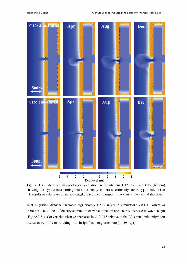
Trang Minh Duong Climate Change impacts on the stability of Small Tidal Inlets
58
Figure 3.30. Modelled morphological evolution in Simulations C12 (top) and C15 (bottom) showing the Type 2 inlet turning into a locatinally and cross-sectionally stable Type 1 inlet when CC results in a decrease in annual longshore sediment transport. Black line shows initial shoreline.
Inlet migration distance increases significantly (~500 m/yr) in simulations C8-C11 where M
increases due to the 100 clockwise rotation of wave direction and the 8% increase in wave height
(Figure 3.31). Conversely, when M decreases in C12-C15 relative to the PS, annual inlet migration
decreases by ~500 m, resulting in an insignificant migration rate (< ~50 m/yr).
C15: Jan-Initial
C12: Jan-Initial Apr
Apr Aug
Aug Dec
Dec
500m
500m
Bed level (m)

Trang Minh Duong Climate Change impacts on the stability of Small Tidal Inlets
59
Figure 3.31. Inlet migration distance for CC driven variations in physical processes at the Type 2 inlet. The migration distance for the PS is also shown (left) for comparison.
Figure 3.32. Changes in mean coastline position (positive = recession) and spatial coastline variability due to CC driven variations in physical processes at the Type 2 inlet. The PS conditions are shown on the left for comparison.
CC driven variations in physical processes and inlet-adjacent coastline
Figure 3.32 shows the variations in mean coastline position and spatial coastline variability
computed for simulations C8-C15. Results show that SLR is the major driver of mean coastline
recession (~120 m recession) as evidenced by the predictions for simulations C10, C11, C14 and

Trang Minh Duong Climate Change impacts on the stability of Small Tidal Inlets
60
C15 relative to other simulations. Spatial coastline variability is significantly higher than that in the
PS only in simulations C8 and C10 (standard deviations of ~35 m relative to ~20 m in the PS),
when both M and P increase.
In summary, a reduction in annual longshore sediment transport, due mainly to CC driven
variations in wave direction, and to a lesser degree in wave height, can increase the stability of an
alongshore migrating Type 2 inlet so much that it changes into a locationally and cross-sectionally
stable Type 1 inlet. CC driven increases/decreases in annual longshore sediment transport can
increase/decrease inlet migration distance by ~100%. SLR does not appear to have any noticeable
impact on the stability of Type 2 inlets. In all situations where the inlet remained a Type 2 inlet
(with individual or combined CC forcing), r values stay in the range 5-20, implying a discrete sub-
category (permanently open and alongshore migrating inlet) not explicitly mentioned in the Bruun
stability criteria. SLR is the main driver of mean coastline recession adjacent to the inlet, which can
be ~120 m, and is largely due to the Bruun effect. A significant increase in the spatial variability of
the coastline relative to the present is predicted when both the tidal prism and annual longshore
sediment transport increase concurrently.
3.3.2.3 Type 3 – Seasonally/Intermittently open, locationally stable inlets (Case study: Maha Oya
river)
CC driven variations in individual forcings and inlet stability
The inlet stability analysis results with CC driven variations in individual forcings are shown in
Table 3.8 and Figure 3.33, which indicate that inlet Type does not change under any of the tested
forcing conditions. Simulation C4, where a 100 clockwise rotation of wave direction decreases M,
shows a marginal increase of r to 8 (from the PS value of 2).
Table 3.8. Individual CC impact simulations of the Type 3 inlet: Forcing, associated changes in
tidal prism P and annual longshore sediment transport M, and predicted future inlet type (ΔHS:
change in wave height; Δθ: change in wave angle; ΔR: change in Riverflow).
CS SLR 1m
ΔHS +8%
ΔHS -8%
Δθ +10O
Δθ -10O
ΔR +40%
ΔR -40%
Potential Change
Inlet Behaviour
C1 x M+,P+ Type 3
C2 x M+ Type 3
C3 x M- Type 3
C4 x M- Type 3
C5 x M+ Type 3
C6 x P+ Type 3
C7 x P- Type 3

Trang Minh Duong Climate Change impacts on the stability of Small Tidal Inlets
61
Figure 3.33. Bruun stability criterion for CC driven variations in individual forcings at the Type 3 inlet. The r value for the PS is also shown (left) for comparison.
The time till inlet closure for the various simulations is shown in Figure 3.34, indicating that the
time till closure is more or less unchanged from its PS value except in C4 where the inlet remains
open for 46 days (i.e. almost a 50% increase relative to the PS).
Figure 3.34. Time till inlet closure for CC driven variations in individual forcings at the Type 3 inlet. The time till closure for the PS is also shown (left) for comparison.
As these simulations were continued only until inlet closure (~one month) coastline recession and
spatial variability computations, which are annual quantities, were not undertaken.
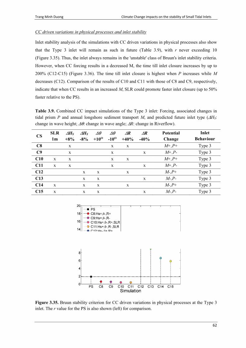
Trang Minh Duong Climate Change impacts on the stability of Small Tidal Inlets
62
CC driven variations in physical processes and inlet stability
Inlet stability analysis of the simulations with CC driven variations in physical processes also show
that the Type 3 inlet will remain as such in future (Table 3.9), with r never exceeding 10
(Figure 3.35). Thus, the inlet always remains in the 'unstable' class of Bruun's inlet stability criteria.
However, when CC forcing results in a decreased M, the time till inlet closure increases by up to
200% (C12-C15) (Figure 3.36). The time till inlet closure is highest when P increases while M
decreases (C12). Comparison of the results of C10 and C11 with those of C8 and C9, respectively,
indicate that when CC results in an increased M, SLR could promote faster inlet closure (up to 50%
faster relative to the PS).
Table 3.9. Combined CC impact simulations of the Type 3 inlet: Forcing, associated changes in
tidal prism P and annual longshore sediment transport M, and predicted future inlet type (ΔHS:
change in wave height; Δθ: change in wave angle; ΔR: change in Riverflow).
CS SLR 1m
ΔHS +8%
ΔHS -8%
Δθ +10O
Δθ -10O
ΔR +40%
ΔR -40%
Potential Change
Inlet Behaviour
C8 x x x M+,P+ Type 3
C9 x x x M+,P- Type 3
C10 x x x x M+,P+ Type 3
C11 x x x x M+,P- Type 3
C12 x x x M-,P+ Type 3
C13 x x x M-,P- Type 3
C14 x x x x M-,P+ Type 3
C15 x x x x M-,P- Type 3
Figure 3.35. Bruun stability criterion for CC driven variations in physical processes at the Type 3 inlet. The r value for the PS is also shown (left) for comparison.

Trang Minh Duong Climate Change impacts on the stability of Small Tidal Inlets
63
Figure 3.36. Time till inlet closure with CC driven variations in physical processes at the Type 3 inlet. The time till closure for the PS is also shown (left) for comparison.
In summary, seasonally/intermittently open inlets will not change Type due to CC driven variations
in forcing/physical processes. The r value remained below 10 in all Type 3 inlet simulations,
implying that for inlet closure, r < 10 is a necessary condition. Despite, not changing Type due to
CC forcing, the time till inlet closure of these inlets may increase by up to 200% when CC results
in a concurrent decrease in annual longshore sediment transport rate and an increase in tidal prism.
In situations where the annual longshore sediment transport rate increases due to CC, SLR could
result in faster inlet closure, decreasing the time till inlet closure by up to 50%.
3.4 Conclusions
A snap-shot simulation approach using a process based coastal area morphodynamic model has
been applied to qualitatively assess CC impacts on the stability of Small Tidal Inlets (STIs). The
modelling approach, which is intended specifically for data poor environments, was applied to
three case study sites representing the main types of STIs: locationally and cross-sectionally stable
inlets (Type 1, Negombo lagoon, Sri Lanka - permanently open, fixed in location); cross-
sectionally stable, locationally unstable inlets (Type 2, Kalutara lagoon, Sri Lanka - permanently
open, alongshore migrating); and locationally stable, cross-sectionally unstable inlets (Type 3,
Maha Oya river, Sri Lanka - seasonally/intermittently open, fixed in location).
Schematized bathymetries that closely follow the key dimensions of the inlet systems were
developed using available data, information and personal communications and used in all model

Trang Minh Duong Climate Change impacts on the stability of Small Tidal Inlets
64
simulations which were undertaken with Delft3D. Morphodynamic model validation simulations
were undertaken using monthly averaged wave and riverflow time series constructed using
available sparse data and reported values. In all 3 cases, successful model validation was achieved
by comparing model results with available satellite images, and where appropriate, with empirical
relationships such as the A-P relationship, Escoffier curve, and the Bruun inlet stability criteria.
The validated models were then used in two sets of simulations with CC modified forcing. The first
set of simulations investigated the impact of CC driven variations in individual system forcings (i.e.
SLR, wave height, wave direction, and riverflow) on STI stability, while the second set
investigated the impact of CC driven variations in key physical processes (i.e. SLR, ebb tidal prism
(including riverflow effects), and annual longshore sediment transport) on STI stability. Worst case
estimates of SLR and CC modified wave/riverflow conditions were obtained from freely available,
coarse resolution published data and used to force the CC impact model simulations. The main
findings are listed below:
• Type 1 and Type 3 models will not change Type even under the most extreme CC forcing
considered here. Type 2 inlets may change into Type 1 when CC results in a reduction in
annual longshore sediment transport, due mainly to CC driven variations in wave direction,
and to a lesser degree in wave height.
• Apart from Type changes, CC driven variations in system forcing and physical processes will
affect the level of inlet stability and some behavioural characteristics. In general, CC driven
variations in annual longshore sediment transport rates appear to be more relevant for future
changes in inlet behaviour, rather than SLR as commonly believed.
• In Type 1 inlets, the Bruun Stability criterion r always remained greater than 50 (i.e. stable).
The level of stability if Type 1 inlets could decrease significantly (by up to two stability
classes in the Bruun inlet stability criterion; from 'good' to 'fair to poor'), due to CC driven
increases in annual longshore sediment transport rate. Mean coastline recession adjacent to the
inlet can be as much as 200 m, while CC driven increases in longshore sediment transport
results in coastline variability that may be twice as much compared to the present.
• In Type 2 inlets, CC driven increases/decreases in annual longshore sediment transport
volume can increase/decrease inlet migration distance by up to 100%. The r value for all
Type 2 inlets (excepting when the inlet changed to Type 1) remained between 5 and 20 (i.e.
unstable). SLR results in a mean coastline recession adjacent to the inlet of ~120 m, and a near

Trang Minh Duong Climate Change impacts on the stability of Small Tidal Inlets
65
doubling of the spatial variability of the coastline relative to the present is predicted when both
the ebb tidal prism and annual longshore sediment transport volume increase concurrently.
• In Type 3 inlets, the r value remained below 10 (i.e. unstable) under all situations simulated,
implying that r < 10 is a necessary condition for inlet closure. The time till closure of these
inlets may increase by up to 200% when CC results in a concurrent decrease in annual
longshore sediment transport rate and an increase in ebb tidal prism. When annual longshore
sediment transport rate increases due to CC, SLR could decrease the time till inlet closure by
up to 50% compared to present conditions.
• Based on the results of this study, inlet Types can be linked with the Bruun stability criteria to
develop a more descriptive inlet classification scheme as shown in Table 3.10.
Table 3.10. Classification scheme for inlet Type and stability conditions.
References
Behrens, D.K., Bombardelli, F.A., Largier, J.L., Twohy, E., 2013. Episodic closure of the tidal inlet at the mouth of the Russian River - A small bar-built estuary in California. Geomorphology, http://dx.doi.org/10.1016/j.geomorph.2013.01.017.
Bruun, P., 1978. Stability of tidal inlets - theory and engineering. Developments in Geotechnical Engineering. Elsevier Scientific, Amsterdam, 510p.
Byrne, R., Gammisch, R., Thomas, G., 1980. Tidal prism-inlet area relations for small tidal inlets. Proceedings of the 21st International Conference on Coastal Engineering, ASCE, New York, pp. 2517-2533.
Chandramohan, P., Nayak, B.U., 1990. Longshore - transport model for South Indian and Sri Lankan coasts. Journal of Waterway, Port, Coastal, and Ocean Engineering, 116, 408-424.
GTZ., 1994. Longhsore sediment transport study for the South West coast of Sri Lanka. Project Report. 25p.
Inlet Type r =P/M Bruun Classification
Type 1
> 150 Good 100 - 150 Fair 50 - 100 Fair to Poor 20 - 50 Poor
Type 2 10 - 20 Unstable
(open and migrating)
Type 2/3 5 - 10 Unstable
(migrating or intermittently closing)
Type 3 0 - 5 Unstable
(intermittently closing)
Trang Minh Duong Climate Change impacts on the stability of Small Tidal Inlets
66
Hemer, M., Fan, Y., Mori, N., Semedo, A., Wang, X.L., 2013. Projected changes in wave climate from a multi-model ensemble. Nature Climate Change, 3, 471-476.
IPCC, 2013. Summary for Policymakers. In: Climate Change 2013: The Physical Science Basis. Contribution of Working Group I to the Fifth Assessment Report of the Intergovernmental Panel on Climate Change [Stocker, T.F., D. Qin, G.-K. Plattner, M. Tignor, S.K. Allen, J. Boschung, A. Nauels, Y. Xia, V. Bex and P.M. Midgley (eds.)]. Cambridge University Press, Cambridge, United Kingdom and New York, NY, USA.
Jarrett, J.T., 1976. Tidal prism – inlet area relationships. Technical Report GITI No.3, CERC, U.S. Army Engineer Waterways Experiment Station, Vicksburg, MS.
Lesser, G.R., Roelvink, J.A., van Kester, J.A.T.M., Stelling, G.S., 2004. Development and validation of a three-dimensional morphological model. Coastal Engineering, 51 (8-9), 883-915.
O’Brien, M.P., 1931. Estuary and tidal prisms related to entrance areas. Civil Engineering, 1(8), 738-739.
Perera, J.A.S.C., 1993. Stabilization of the Kaluganga river mouth in Sri Lanka. M.Sc Thesis Report. International Institute for Infrastructural Hydraulic and Environmental Engineering, Delft, The Netherlands, 97p.
Ranasinghe, R., Swinkels, C., Luijendijk, A., Roelvink, D., Bosboom, J., Stive, M., Walstra, D., 2011. Morphodynamic upscaling with the MORFAC approach: Dependencies and sensitivities. Coastal Engineering, 58, 806-811.
Ranasinghe, R., Duong, T.M., Uhlenbrook, S., Roelvink, D., Stive, M., 2013. Climate change impact assessment for inlet-interrupted coastlines. Nature Climate Change, 3, 83-87, DOI.10.1038/NCLIMATE1664.
Roelvink, J.A., 2006. Coastal morphodynamic evolution techniques. Coastal Engineering, 53, 277-287.
University of Moratuwa., 2003. Engineering study on the feasibility of dredging the Negombo Lagoon to improve water quality. Final Report. Part II: Technical & Enviromental Feasibility.
van Koningsveld, M., Mulder, J.P.M., 2004. Sustainable coastal policy developments in the Netherlands. A systematic approach revealed. Journal of Coastal Research, 20(2), 375-385. West Palm Beach (Florida), ISSN 0749-0208.
van Rijn, L.C., 1993. Principles of sediment transport in rivers, estuaries and coastal seas. Part 1. AQUA Publications, NL. 700p.
Wijeratne, E.M.S., 2002. Sea level measurements and coastal ocean modelling in Sri Lanka. Proceedings of the 1st scientific session of the National Aquatic Resources Research and Development Agency, Sri Lanka. 18p.
Zubair, L., Chandimala, J., 2006. Epochal changes in ENSO – streamflow relationships in Sri Lanka. Journal of Hydrometeorology, 7(6), 1237-1246.

Trang Minh Duong Climate Change impacts on the stability of Small Tidal Inlets
67
CHAPTER 4
ASSESSING CLIMATE CHANGE IMPACTS ON THE STABILITY OF SMALL TIDAL INLETS IN DATA RICH ENVIRONMENTS
4.1 Introduction
This Chapter demonstrates the application of the process based snap-shot modelling approach for
data rich environments proposed in Section 2.4.1. The approach is applied to the 3 case study sites
representing the 3 main STI types described Section 3.2.1.
Following Ruessink and Ranasinghe's (2014) ensemble modelling approach described in
Section 2.4.1 and Figure 2.10 therein, a modified framework shown in Figure 4.1 was adopted in
this study. The main deviations from the comprehensive framework suggested by Ruessink and
Ranasinghe (2014) are: (1) only one GHG scenario (the high end A2 scenario) was considered, and
(2) only one RCM was used. Thus, the GHG and RCM uncertainties are not accounted for in this
study. This is mainly due to budgetary constraints of the study and therefore was unavoidable.

Trang Minh Duong Climate Change impacts on the stability of Small Tidal Inlets
68
Figure 4.1. Modelling framework adopted in the present study following the comprehensive ensemble modelling framework proposed by Ruessink and Ranasinghe (2014).
GHG scenario
(Only A2)
CCAM
Regional/catchment scale coastal forcing models (waves, riverflow)
Local scale coastal impact models (Delft3D)
STEP 1: GHG scenario
STEP 2: To account for GCM uncertainty (GCM ensemble)
Dynamic downscaling
Bias correct for present time slice
STEP 3: RCM
STEP 4: Validate for present time slice and apply for future times to obtain projections to force coastal impact models with
STEP 5: Validate for present time slice and apply for future times to obtain full range of potential impacts
ECHAM
GFDL

Trang Minh Duong Climate Change impacts on the stability of Small Tidal Inlets
69
4.2 Dynamic downscaling
All downscaled climate variables were derived from the stretched grid model CCAM (Conformal
Cubic Atmospheric Model) which is owned and operated by CSIRO, Australia. CCAM is a semi-
implicit, semi-Lagrangian atmospheric climate model based on a conformal cubic grid (McGregor
and Dix, 2008). Although CCAM is a global atmospheric model, it allows a variable resolution
grid which enables a finer grid resolution over the target area at the expense of a coarser resolution
on the opposite side of the globe. In this way, CCAM can be used for regional climate experiments
without imposing lateral boundary conditions. The variable resolution grid used to derive the
downscaled climate variables over Sri Lanka for this study is shown in Figure 4.2. In this
application CCAM employed 18 vertical levels (ranging from 40 m to 35 km. The grid used in the
CCAM application for this study resulted in a resolution of about 65 km over Sri Lanka. The model
was forced with Sea Surface Temperatures taken from two of the CMIP3 General Circulation
Models (ECHAM and GFDL) which performed well in the target area. CCAM output including
winds, surface temperature, atmospheric pressure, radiation, ocean temperature etc. was thus
obtained for the 1981-2000 (present) and 2081-2100 time slices at a temporal resolution of 6 hours.
Figure 4.2. The variable resolution conformal cubic grid in the CCAM simulations.

Trang Minh Duong Climate Change impacts on the stability of Small Tidal Inlets
70
4.3 Regional/catchment scale coastal forcing models
4.3.1 Riverflow
The CCAM output over Sri Lanka was used in a hydrologic model to derive riverflow estimates for
the present (1981-2000) and future (2081-2100) (Mahanama and Zubair, 2011). The 6-hourly
surface meteorological forcings used included shortwave radiation, longwave radiation, total
precipitation, convective precipitation, surface pressure, air temperature, specific humidity, and
wind for the two different periods. The hydrologic model used was the Catchment Land Surface
Model (CLSM: Koster et al., 2000; Ducharne et al., 2000). CLSM is a macroscale hydrologic
model that balances both surface water and energy at the Earth’s land surface. One distinguishing
characteristic of CLSM is that it considers irregularly shaped, topographically delineated,
hydrologic catchments as the fundamental element on the land surface for computing land surface
processes. The CLSM has already been successfully implemented in Sri Lanka (Mahanama et al.,
2008) using bias corrected reanalysis meteorological forcings. For this study, the CLSM was forced
in offline mode using the CCAM downscaled surface meteorological forcings to generate
riverflows into the 3 case study lagoons.
Available gridded precipitation data were used for bias correcting the downscaled ECHAM
and GFDL precipitation hindcasts for the present time slice, which were then used in CLSM
to simulate riverflows. Observed monthly riverflows from 22 gauge stations across Sri Lanka
for the period 1979-1993 were used for validating CLSM for the hindcast period 1981-2000.
As the ECHAM and GFDL projections for the 3 case study lagoons were very similar, only
GFDL projections were used to construct the annual cycle of riverflows to use as future
forcing in the Coastal impact model, Delft3D. Here Delft3D was used with a MORFAC of 13
to ensure the representation of the spring-neap cycle in the CC impact assessments (see
Section 4.4.1 below), and therefore, 13-day averaged riverflows were used to construct the
average annual riverflows (Figure 4.3) to force the process based snap-shot model simulations
described below in Section 4.4. In general, by 2100 (relative to the present), riverflow is
projected to decrease by about 41% and 32% at Negombo lagoon and Kalutara lagoon
respectively, while an increase of about 72% is indicated for Maha Oya river.

Trang Minh Duong Climate Change impacts on the stability of Small Tidal Inlets
71
Figure 4.3. Contemporary and year 2100 riverflow time series for Negombo lagoon (left), Kalutara lagoon (middle), and Maha Oya river (right).
4.3.2 Waves
CCAM winds were used to force two nested spectral wave models for 1981-2000 (hindcast) and
2081-2100 (future) time slices (Bamunawala, 2013). Due to the similarity between CCAM
downscaled ECHAM and GFDL winds in the study area, only CCAM-GFDL winds were used in
this analysis. For the generation of far field waves, WAVEWATCH III (Tolman, 2009) was used
(Latitudes N220-S70; Longitudes E650-E950). SWAN (Booij et al., 1999) was used in the near field
from about 50 m depth to the coastline extending from Galle to Puttalam along the SW coast (see
Figure 3.1 for locations). Modelled wave conditions for the hindcast period were compared against
available deep water wave data off Colombo. The bias correction required to ensure a good
model/data comparison was then determined and applied to the future projected wave conditions
with the commonly adopted assumption that present-day biases between model and reality will
remain the same in future (Charles et al., 2012; Wang et al., 2014). SWAN model output was then
extracted at 20 m depth offshore of the 3 case study sites to use as boundary forcing in the
process based snap-shot model simulations described in Section 4.4 below. As the process
based model Delft3D was used with a MORFAC of 13 to ensure the representation of the
spring-neap cycle in the CC impact assessments (see Section 4.4.1 below), 13-day averaged
wave heights and directions were used to construct the average annual wave conditions for
model forcing (Figure 4.4).

Trang Minh Duong Climate Change impacts on the stability of Small Tidal Inlets
72
Figure 4.4. Contemporary and year 2100 wave time series (at 20m depth) for Negombo lagoon (left), Kalutara lagoon (middle), and Maha Oya river (right). Significant wave height (Hs) (top),
mean wave direction (D = θ) (bottom).
4.4 Coastal Impact modelling
The process based coastal area model Delft3D was used for all simulations undertaken in this
study. The model is fully described by Lesser et al., (2004) and is therefore not described here. For
the 3 case study applications of the model in this study, identical wave and flow domains which
were large enough to avoid any boundary problems affecting the area of interest were created
(Figure 4.5). High resolution (~10x10 m) grid cells were used in the (approximate) surf zone and
inlet channel for all 3 study areas to ensure that key physical processes in the vicinity of the inlet
entrance and channel were accurately resolved by the model. Good measured bathymetries were
available for all 3 case study sites.

Trang Minh Duong Climate Change impacts on the stability of Small Tidal Inlets
73
Figure 4.5. Wave/flow grids for Negombo (left), Kalutara (middle) and MahaOya (right)
4.4.1 Model validation
Hydrodynamic validation
First the models were validated against measured water level and velocity data inside the lagoons.
Water level and velocity measurements for Negombo lagoon were available from a previous study.
Two pressure sensors were deployed in Kalutara lagoon and Maha Oya river to collect water level
data for this study specifically. Unfortunately however, due to problems with data acquisition,
water level data at Kalutara lagoon was only captured intermittently, while the sensor deployed at
Maha Oya river was lost. Therefore, hydrodynamic model validation could only be undertaken for
Negombo and Kalutara lagoons. The hydrodynamic validation simulations were undertaken with
only tidal and riverflow forcing as wave effects are minimal within the 3 case study STIs. Tidal
forcing constituted of astronomical tides composed of the 6 main tidal constituents in the area (M2,
S2, N2, K2, K1, O1), and riverflow was introduced as a time series based on available
measurements. Morphological updating was turned off in these short-term simulations. The
validation periods and data are shown in Table 4.1. The measurement locations are shown in
Figure 4.6. A Chezy friction coefficient of 65m1/2/s, eddy viscosity of 1m2/s and hydrodynamic
time step of 6 seconds were adopted in all 3 hydrodynamic validation simulations.
Bed level (m)

Trang Minh Duong Climate Change impacts on the stability of Small Tidal Inlets
74
Table 4.1. Data used for hydrodynamic model validation at the case study sites.
STI System Data type Data period Negombo lagoon Water level 01 - 30 Oct 2002
Velocity 02 - 03 Oct 2002 Kalutara lagoon Water level 13 - 26 Feb 2013
Figure 4.6. Measurement locations of model validation data in Negombo lagoon (left) and Kalutara lagoon (right). Filled white circles: water level observation points (Negombo - S1: ocean side, S3: inside lagoon; Kalutara - K1: inside lagoon). Asterisks: velocity observation points (Negombo - CM1: ocean side, CM2: inside lagoon).
Table 4.2. Model/data comparison statistics for the hydrodynamic validation simulations.
Negombo lagoon
Water level S1 S3
RMSE R2 RMSE R2
0.0325 0.9747 0.0312 0.8355
Current CM1 CM2
Current velocity 0.1027 0.7319 0.0598 0.4397
Current direction 10.17 0.6890 14.59 0.5628
Kalutara lagoon
Feb 15 Feb 20 Feb 23
Water level K1 K1 K1
RMSE R2 RMSE R2 RMSE R2
0.1155 0.8668 0.0776 0.9872 0.0538 0.8747

Trang Minh Duong Climate Change impacts on the stability of Small Tidal Inlets
75
The model/data comparisons for Negombo and Kalurara lagoons (Figures 4.7 and 4.8, and
Table 4.2) are reasonably good, providing sufficient confidence in the models to proceed with the
morphodynamic simulations.
Figure 4.7. Model/data comparisons of water levels and currents (magnitude and direction) at Negombo lagoon.

Trang Minh Duong Climate Change impacts on the stability of Small Tidal Inlets
76
Figure 4.8. Model/data comparison of water levels at Kalutara lagoon
Morphodynamic validation
Morphodynamic validation was achieved in much the same way as it was done with the data poor
approach adopted in Chapter 3. For Negombo lagoon and Kalutara lagoon, one year
morphodynamic simulations were undertaken, while for Maha Oya river the morphodynamic
simulation was continued only until the inlet closed. Models were forced with astronomical tides
for which constituents were obtained from Wijeratne (2002). All model parameter values, except
the MORFAC value and the Hydrodynamic spin up time, were the same as those indicated in
Table 3.2. A MORFAC of 13 was used in these simulations in order to capture two spring-neap
cycles (29 days) of hydrodynamic forcing within a 1 year morphodynamic simulation. A
hydrodynamic spin up time of 24 hrs was used in these simulations to ensure that model velocities
were stable before sediment transport and morphological computations were undertaken. Modelled
bed level changes and satellite images for the 3 systems are shown in Figures 4.9-4.11. Modelled
and measured (reported) annual LST (or M) in the vicinity of the 3 inlets are shown in Table 4.3. M
was calculated following the approach described in Section 3.2.5.
Table 4.3. Modelled and measured (reported) annual LST (M) in the vicinity of the 3 case study inlets, the modelled Bruun criterion r and corresponding Bruun stability classification and inlet Type following Table 3.10.
STI system Reported M
(m3/yr) Modelled M
(m3/yr) r =
P/M Bruun stability classification
Inlet Type
Negombo Lagoon
20,000 S 42,000 S 221 Good 1
Kalutara Lagoon
500,000 S 562,000 S 11 Unstable 2
Maha Oya River
500,000 N 450,000 N 1 Unstable 3

Trang Minh Duong Climate Change impacts on the stability of Small Tidal Inlets
77
Figure 4.9. Satellite images (top (source: Landsat)) and validation model results (bottom) of the annual bed level evolution of Negombo lagoon, showing the observed and modelled locationally and cross-sectionally stable inlet behaviour. The black line in the model results indicates the initial shoreline position.
Jan 2014 Apr 2014 Aug 2014 Dec 2014
Jan (initial)
Apr Aug Dec
Bed level (m)
500m

Trang Minh Duong Climate Change impacts on the stability of Small Tidal Inlets
78
Figure 4.10a. Satellite images (top (source: Landsat)) and validation model results (bottom) of the annual bed level evolution of the Kalutara lagoon inlet, showing the observed and modelled locationally unstable and cross-sectionally stable inlet behaviour with the model correctly reproducing the observed southward migration of about 500 m/yr (see also Figure 4.10b). The black line in the model results indicates the initial shoreline position.
Sep 1975 Jan 1977 Jun 1978 Feb 1980
500m
Bed level (m)
Apr Aug Dec Jan (initial)

Trang Minh Duong Climate Change impacts on the stability of Small Tidal Inlets
79
Figure 4.10b. Modelled inlet migration distance and speed through the 1 year validation simulation of Kalutara lagoon inlet showing that the model correctly reproduces observed southward (negative = southward) migration rate of ~500 m/yr and higher migration speeds during the SW monsoon.
Figure 4.11a. Satellite images (top (source: Landsat)) and validation model results (bottom) showing the bed level evolution of the Maha Oya river inlet, showing the observed and modelled locationally stable and cross-sectionally unstable inlet behaviour. The white dashed circles in the satellite images indicate inlet closed situations. Black line in model results show initial coastline.
Aug 2006 Sep 2006 (SW) Oct 2006 Nov 2006
300m
Bed level (m)
Initial 15 days 25 daysClosure 45 days

Trang Minh Duong Climate Change impacts on the stability of Small Tidal Inlets
80
Figure 4.11b. Time evolution of inlet cross-sectional area in the validation simulation of Maha Oya river showing that the model correctly reproduces observed inlet closure.
In summary, the above results show that the model is able to reproduce contemporary observed
behaviour of the 3 case study STIs providing sufficient confidence in the model to proceed with CC
impact assessments.
4.4.2 CC impact assessment
For each STI system, the validated model was then implemented via snap-shot simulations to
investigate future CC impacts on the system. These simulations were also undertaken for the same
duration as the validation simulations, or, in the case of Maha Oya river, until inlet closure
occurred. For each STI, CC modified riverflow and wave forcing were implemented using the
projected forcing shown in Figures 4.3 and 4.4. A worst case SLR of 1m (by 2100 relative to the
present) was applied at all 3 systems. The tidal forcing of all CC impact simulations were the same
as that used in the respective validation simulations.
Due to the spatially non-uniform bathymetries of the systems, SLR driven basin infilling was
implemented differently compared to the simple spatially uniform raising of the lagoon/inlet bed
level method used in the flat-bed schematized models described in Chapter 3. Here, the bed levels
of the initial measured bathymetry were changed to accommodate the basin infill volume
(calculated in exactly the same way as described in Section 2.4.1, i.e. total infill volume = 0.5 x
SLR x Ab, where Ab = surface area of lagoon, or basin) such that the shape of the present and future
Closure 45 days

Trang Minh Duong Climate Change impacts on the stability of Small Tidal Inlets
81
basin hyspometry curves were more or less the same. Basin hypsometry is the relationship between
the basin depth (hb) (measured from surface to the bottom, elevation = 0 at surface) and the basin
area (Ab) (also measured from bottom to surface, with area = 0 at the bottom) (Boon and Byrne,
1981). To estimate the bed level changes required to represent basin infilling, first it is assumed
that at all grid points:
ℎ , = ℎ , + − ∆ℎ (4.1)
where: Δh is assumed to follow the general depth transfer function given by,
∆ℎ = ℎ , + (4.2)
where: a' is a coefficient, of which the optimal value is found via iteration. Subscripts 'p' and 'f'
represent present and future respectively.
As an example, the year 2100 basin hypsometry curve calculated for Kalutara lagoon using the
above approach is shown in Figure 4.12, together with the contemporary hypsometry curve.
Figure 4.12. Present and future (year 2100) basin hypsometry curves indicative of the implemented bed level changes in Kalutara lagoon to represent SLR driven basin infilling.

Trang Minh Duong Climate Change impacts on the stability of Small Tidal Inlets
82
Negombo Lagoon
The modelled future morphological changes over one year for the Type 1 Negombo lagoon are
shown in Figure 4.13. For easy comparison, the validation simulation results for this STI shown in
Figure 4.9 are also reproduced in Figure 4.13 (top panels). Model results show that this STI will
remain a locationally and cross-sectionally stable inlet by 2100. The r value however decreases to
75, from its present value of 221. According to Bruun's inlet stability classification, this implies
that the level of stability of the inlet will decrease from 'good' to 'fair to poor'.
Figure 4.13. Modelled morphological changes for Negombo lagoon over a one year period; under contemporary forcing conditions (top) and CC modified year 2100 forcing conditions (bottom). Kalutara lagoon
The modelled future morphological changes over one year for the Type 2 Kalutara lagoon are
shown in Figure 4.14, together with corresponding validation simulation results. Model results
Apr Aug Dec
500m
Bed level (m)
Apr Aug Dec
500m
Jan (initial)
Jan (initial)

Trang Minh Duong Climate Change impacts on the stability of Small Tidal Inlets
83
show that Kalutara lagoon will remain a permanently open, alongshore migrating Type 2 STI by
year 2100. However the migration distance doubles to ~1200 m, while the r value decreases to 6
from its present value of 11. These changes can be directly attributed the future increase in
southward M due the CC driven clockwise rotation of waves (see Figure 4.4).
Figure 4.14. Modelled morphological changes for Kalutara lagoon over a one year period; under contemporary forcing conditions (top) and CC modified year 2100 forcing conditions (bottom). Maha Oya river
The modelled future morphological changes for the Type 3 Maha Oya river are shown in
Figure 4.15, together with corresponding validation simulation results. Model results show that this
500m
500m
Bed level (m)
Apr Aug Dec Jan (initial)
Apr Aug Dec Jan (initial)

Trang Minh Duong Climate Change impacts on the stability of Small Tidal Inlets
84
STI will remain an intermittently open, locationally stable Type 3 STI by year 2100. However the
time until inlet closure increases by more than 50% from its modelled present value of 45 days to
78 days, while the r value slightly increases to 5 from its present value of 1. These changes in
system behaviour is due to the combined effect of the future increase in annual riverflow (see
Figure 4.3) and the smaller northward M resulting from the CC driven clockwise rotation of waves
(see Figure 4.4).
Figure 4.15. Modelled morphological changes for Maha Oya river until inlet closure; under contemporary forcing conditions (top) and CC modified year 2100 forcing conditions (bottom).
Bed level (m)
300m
300m
Initial 15 days 25 daysClosure 45 days
Initial 15 days 25 daysClosure 78 days

Trang Minh Duong Climate Change impacts on the stability of Small Tidal Inlets
85
4.4.3 Relative contributions of CC driven variations in system forcing to inlet stability
For each case study, four additional simulations where CC forcing was sequentially removed
(Simulations R2-R5; R1 being the above discussed 'all inclusive' CC impact simulation) were
undertaken to investigate the relative contribution of the different CC forcings to future inlet
stability. The CC forcings implemented in each simulation are shown in Table 4.4. Note that when
CC modified future forcing is not used in a certain simulation (e.g. future riverflow Rf in R2), the
present riverflow is still used for the year 2100 snap-shot simulation (i.e. representing a scenario
where there is no change in riverflow due to CC). Also, basin infilling was not included in
simulations that excluded SLR (i.e. R5). When SLR is implemented (Simulations R1-R4), it was
specified as 1m. This set of simulations can be used to determine the effect of CC driven changes
in each of the system forcings on future STI behaviour. For example, the difference between R2
and R1 would be indicative of the isolated effect CC driven changes in annual riverflow would
have on STI behaviour, while differences between R5 and R1 would provide insights on the effect
of SLR.
Table 4.4. Forcing conditions implemented in the different CC forcing simulations. Subscript 'f' indicates future conditions.
SLR HSf ,θf Rf
R1 x x x
R2 x x
R3 x x
R4 x
R5 x x
The main results from this set of simulations are summarised in Table 4.5. The results of the
validation simulation (R1) are also shown for easy comparison.
Table 4.5. Model predicted year 2100 STI types and inlet behavioural characteristics in response to different CC forcings.
Negombo
lagoon Kalutara lagoon Maha Oya river
Simulation r Type r Migration
distance(m)Type r
Time till closure(days)
Type
R1 75 Type 1 6 1210 Type 2 5 78 Type 3 R2 82 Type 1 7 1183 Type 2 4 72 Type 3 R3 128 Type 1 7 914 Type 2 1 65 Type 3 R4 142 Type 1 9 851 Type 2 1 65 Type 3 R5 83 Type 1 6 1067 Type 2 4 72 Type 3

Trang Minh Duong Climate Change impacts on the stability of Small Tidal Inlets
86
The results in Table 4.5 indicate that the presence or absence of CC driven changes in any one
system forcing is not capable of changing the Type of any of the 3 case study STIs.
For Negombo lagoon, the results indicate that CC driven changes in wave conditions (in this case
with an associated increase in M) have the largest impact on inlet stability, accounting for almost
70% of overall CC modified r value of 75 (by comparing r for R1, R3 and R4). Comparison of
results for R1, R2 and R5 indicate that CC driven variations in riverflow and SLR both appear to
have smaller but similar contributions to the overall CC effect on inlet stability (~10%
contribution).
For Kalutara lagoon, the variations among r values computed for the 5 simulations are insignificant
and stay within the 5 < r < 10 range. Nevertheless, the variations in migration distance indicate that
the phenomenon which contributes most to the 1210 m of migration due to combined CC forcing
(R1) is CC driven variations in wave conditions (R3, 25% contribution to the overall migration
distance).
At Maha Oya, while both the r value and time to closure for all simulations vary very little, the
biggest drops in both diagnostics are attributable to CC driven variations in wave conditions (by
comparing R1, R3 and R4).
The above results show that SLR appears not to be the main contributor to future CC driven
variations in inlet stability and/or behaviour at any of the 3 case study STIs.
4.5 Conclusions
A snap-shot simulation approach using the process based coastal area morphodynamic model
Delft3D has been applied to assess CC impacts on the stability of Small Tidal Inlets (STIs). The
modelling approach was applied to three case study sites representing the main types of STIs:
locationally and cross-sectionally stable inlets (Type 1, Negombo lagoon, Sri Lanka - permanently
open, fixed in location); cross-sectionally stable, locationally unstable inlets (Type 2, Kalutara
lagoon, Sri Lanka - permanently open, alongshore migrating); and locationally stable, cross-
sectionally unstable inlets (Type 3, Maha Oya river, Sri Lanka - seasonally/intermittently open,
fixed in location). Future CC modified wave and riverflow conditions were derived from a regional
scale application of spectral wave models (WaveWatch III and SWAN) and catchment scale
applications of a hydrologic model (CLSM) respectively, both of which were forced with IPCC

Trang Minh Duong Climate Change impacts on the stability of Small Tidal Inlets
87
GCM output dynamically downscaled to ~65 km resolution over the study area with the Conformal
Cubic Atmospheric Model CCAM.
The coastal impact model used in this study, Delft3D, was successfully validated for contemporary
conditions using short-term hydrodyamic measurements and the general morphological behaviour
observed in satellite images of the study sites. Subsequent CC impact simulations undertaken with
the validated models forced with 2100 projected SLR, waves and riverflows indicate the following:
• None of the 3 case study STIs will change Type by the year 2100.
• By the end of the 21st century, the level of stability of the Negombo lagoon, as indicated by
the Bruun criterion r, will decrease from 'Good' to 'Fair to poor'. The level of (locational)
stability of the Kalutara lagoon, as indicated by the doubling of the annual migration
distance, will also decrease. At Maha Oya river, the time till inlet closure will increase by
more than 50%, indicating an increase in the level of stability of this inlet.
• CC driven variations in wave conditions, and resulting changes in the annual longshore
sediment transport, is the main contributor to the overall CC effect on the stability of all 3
STIs. SLR and CC driven variations in riverflows play only a rather secondary role.
The results obtained by applying the 'data rich' approach to the 3 case study sites are, to a large
extent, in agreement with those obtained from the more generically applied 'data poor' approach
presented in Chapter 3.
References
Bamunawala, R. M. J., 2013. Impact of climate change on the wave climate of Sri Lanka. M.Sc Thesis, University of Moratuwa, Sri Lanka. 55p.
Boon, J. D., Byrne, R. J., 1981. On basin hypsometry and the morphodynamic response of coastal inlet sytems. Marine Geology, 40, 27-48.
Booij N., Ris, R.C., Holthuijsen L.H., 1999. A third generation wave model for coastal regions. Part 1: model description and validation. Journal of Geophysical Research 104 (C4), 7649-7666.
Charles, E., Idier, D., Delecluse, P., Deque, M., Le Cozannet, G., 2012. Climate change impact on waves in the Bay of Biscay. Ocean Dynamics, 62, 831-848.
Ducharne, A., Koster, R. D., Suarez, M. J., Stieglitz, M., Kumar, P., 2000. A catchment-based approach to modeling land surface processes in a GCM, Part 2, Parameter estimation and model demonstration. Journal of Geophysical Research, 105, 24823-24838.

Trang Minh Duong Climate Change impacts on the stability of Small Tidal Inlets
88
Koster, R. D., Suarez, M. J., Ducharne, A., Stieglitz, M., Kumar, P., 2000. A catchment-based approach to modeling land surface processes in a GCM, Part 1, Model Structure. Journal of Geophysical Research, 105, 24809-24822.
Lesser, G., Roelvink, J.A., Van Kester, J.A.T.M., Stelling, G.S., 2004. Development and validation of a three-dimensional morphological model. Coastal Engineering 51, 883-915.
Mahanama, S. P. P., Koster, R. D., Reichle, R. H., Zubair, L., 2008. The Role of Soil Moisture Initialization in Sub-seasonal and Seasonal Streamflow Prediction - A Case Study in Sri Lanka. Advances in Water Resources, 31, 1333-1343.
Mahanama, S.P.P., Zubair, L., 2011. Production of streamflow estimates for the Climate Change Impacts on Seasonally and Intermittently Open Tidal Inlets (CC-SIOTI) Project. FECT Technical Report 2011-01: Foundation for Environment, Climate and Technology, Digana Village, October, 2011. 20p.
McGregor, J., Dix, M., 2008. An updated description of the conformal cubic atmospheric model. In: High resolution Simulation of the Atmosphere and Ocean (Eds. Hamilton, K., Ohfuchi, W.) Springer, pp. 51-76.
Ruessink, B.G., Ranasinghe, R., 2014. Beaches. In: Coastal environments and Global change (Eds. Masselink, G., Gehrels, R.). Wiley, pp. 149-176.
Tolman, H., 2009. User manual and system documentation of WAVEWATCH III™ version 3.14. NOAA/NWS/NCEP/MMAB Technical Note 276, 194 pp + Appendices. (URL http://polar.ncep.noaa.gov/waves/wavewatch/).
Wang, L., Ranasinghe, R., Maskey, S., van Gelder, P. H. A. J. M., Vrijling, J. K., 2015. Comparison of empirical statistical methods for downscaling daily climate projections from CMIP5 GCMs: a case study of the Huai River Basin, China. International Journal of Climatology, DOI 10.1002/joc.4334.
Wijeratne, E. M. S. (2002). Sea level measurements and coastal ocean modelling in Sri Lanka. Proceedings of the 1st scientific session of the National Aquatic Resources Research and Development Agency, Sri Lanka. 18p.

Trang Minh Duong Climate Change impacts on the stability of Small Tidal Inlets
89
CHAPTER 5
A REDUCED COMPLEXITY MODEL TO OBTAIN RAPID PREDICTIONS OF CLIMATE CHANGE IMPACTS ON THE STABILITY OF SMALL TIDAL INLETS
5.1 Introduction
One of the main shortcomings of the process based snap-shot modelling approach discussed thus
far in this thesis is its inability to provide any insights on the temporal evolution of STI stability in
response to climate change (CC) modified system forcing. Another important issue is that the
application of sophisticated process based models such as Delft3D under any situation requires a
high level of specific expertise in using the model. Such expertise is uncommon among frontline
coastal zone managers and planners who have to deal with CC impacts on coasts on a regular basis.
In fact, frontline managers/planners appear to prefer simple models that can be used with a very
limited knowledge of mathematical modelling but are still able provide reliable and rapid
assessments of system behaviour (Ranasinghe at al., 2012; Wainwright et al., 2015). An easy-to-
use reduced complexity (or aggregated) model that captures the physics governing inlet stability
and is capable of providing rapid and reliable qualitative assessments of how inlet stability may
evolve in time would address both of the above issues. Reduced complexity models have
previously been successfully developed and used to simulate river morphodynamics (Murray and
Paola, 1994, 1997), coastline change (Ashton and Murray, 2001; Ranasinghe et al., 2013) and inlet-
basin systems (Stive and Wang, 2003; van Goor et al., 2003). In this chapter, a reduced complexity
model to predict CC effects on STI stability is developed and applied to the three case studies STIs
described in Chapters 3 and 4.

Trang Minh Duong Climate Change impacts on the stability of Small Tidal Inlets
90
5.2 Governing processes
Under contemporary conditions, inlet stability is governed primarily by two processes: (1) annual
ambient longshore sediment transport in the vicinity of the inlet (M), and (2) flow through the inlet
during ebb. The latter will not only include the ebb tidal prism (volume of water flowing out of the
estuary/lagoon due to tidal forcing alone) but also riverflow effects. For convenience, hereon, the
ebb flow due to the combined effect of both of these processes will be referred to as tidal prism (P).
CC driven variations in wave conditions and riverflow can modify both M and P in future.
5.2.1 Climate change and longshore sediment transport
At the most basic level, longshore sediment transport (LST) rate is a function of sediment size (D50)
and breaking wave height (Hb) and angle (θb). There are several bulk equations (e.g. CERC, 1984;
Bayram et al., 2007) that express LST as a predominant function of these parameters. Kamphuis
(1991) presented an LST equation which, apart from these parameters, also includes the effect of
the surf zone bed slope (Eq. 5.1).
= 2.27 . . . . (2 ) (5.1)
where: is immersed mass of sediment transported alongshore (kg/s), is the significant wave
height at the breaker (m), is the wave angle at the break point (degrees), is the peak wave
period (s), = ℎ / is the beach slope, ℎ is the water depth at break point (m), is the
distance from the shoreline to the break point (m), and is the median grain size (m),
is related to the volume via = ( )( ) , where: is the sediment transport volume
(m3/s), is the density of sand (kg/m3), is the fluid density (kg/m3), is porosity of sand.
This equation has been shown to perform remarkably well on large data sets (Kamphuis, 1991;
Schoonees and Theron, 1996). Milhomens et al. (2013) re-assessed the commonly used CERC,
Bayram and Kamphuis LST equations using a comprehensive database containing laboratory and
field data and proposed new improved versions for all 3 equations. Among these however, the
improved Kamphuis equation (Eq. 5.2) gave the best agreement with data.
, = 0.149 . . . . . (2 ) (5.2)

Trang Minh Duong Climate Change impacts on the stability of Small Tidal Inlets
91
It is now well known that CC will result in sea level rise (SLR) and modified deepwater wave
heights and directions around the world (Hemer et al., 2013). Such CC driven modifications in
offshore wave conditions will also affect breaking wave properties Hb and θb. Furthermore, SLR
will result in waves breaking closer to the shoreline and hence a steeper surf zone slope
(higher mb). All of these CC effects can be accounted for by using Eq. 5.2 with appropriate CC
forcing.
5.2.2 Climate change and tidal prism
As mentioned above, the total ebb tidal prism can be divided into two parts:
= + (5.3)
where: Pt is the ebb flow due to tide only and R is the riverflow volume during ebb. In small
estuary/lagoon system where it can safely be assumed that there is no phase lag in tidal elevation
within the system (Keulegan, 1951), Pt can be expressed as:
= × (2 × ) (5.4)
where: Ab is the surface area of the estuary/lagoon and ab is the mean tidal amplitude inside the
estuary/lagoon.
As STIs do not usually contain extensive tidal flats or salt marshes, it can be assumed that SLR will
not change Ab. The lagoon tidal range ab then is a function of the ocean tidal range and tidal
attenuation across the inlet channel (Keulegan, 1951; van der Kreeke, 1988; Ranasinghe and
Pattiaratchi, 2000). CC is not expected to affect ocean tides in any significant way and hence CC
will only affect ab via changes in tidal attenuation. Inlet channel dimensions such as length, width
and depth will directly affect the degree of tidal attenuation (Keulegan, 1951).With CC, the
competing effects of SLR and basin infilling (Ranasinghe et al., 2013) will result in increasing inlet
depth by half the amount of SLR. This will decrease tidal attenuation, thus increasing Pt.
Keulegan (1951) presented an analytical solution to calculate tidal attenuation at inlets which can
be used to calculate the CC modified Pt at STIs. The starting point for this approach is Eq. 5.5
which describes the difference in water level across a tidal inlet:
= ℎ − ℎ (5.5)

Trang Minh Duong Climate Change impacts on the stability of Small Tidal Inlets
92
where: ℎ is the water level inside the basin (m), ℎ is the water level at the sea (m), is the
coefficient of filling or repletion, given by the Eq. 5.6 below:
=
(5.6)
where: is the tidal period (s), is the tidal amplitude at the sea (m), is the cross-sectional area
of the connecting channel (m2), is the basin surface area (m2), is the gravitational acceleration
(m2/s), is the hydraulic radius of the channel (m), is the friction coefficient, is the length of
the connecting channel (m), is the coefficient resulting from the velocity distribution over the
channel cross section.
As Eq. 5.5 is an implicit equation, after some mathematical manipulations and approximations for
sinusoidal tidal oscillations, Keulegan (1951) arrived at Eq. 5.7, which is explicit.
= (5.7)
where: is the tidal amplitude inside the basin (m), and sinτ is a function of K.
Keulegan (1951) further provided look-up tables for sinτ vs K. As the latter can easily be estimated
for a given system from Eq. 5.6, ab can then be calculated for a given ocean tidal amplitude ao,
which is generally known. This ab can then be used, along with Ab, in Eq. 5.4 to compute Pt, which
can be combined with a known riverflow (per ebb phase) to calculate P using Eq. 5.3. It is noted
that Keulegan's (1951) approach does not allow ab to be greater than ao (i.e. always < 1) and
therefore is not suitable for situations where tidal resonance may amplify ab. However, for tidal
resonance to occur the ratio length of basin/tidal wave length should be 0.25 (Dronkers, 1964). For
STIs therefore this situation is unlikely to occur. For example, the length of basin/tidal wave length
ratio of the 3 STIs investigated here ranges between 0.002 and 0.078.
5.3 The model
The basic structure of the reduced complexity model developed in this study is shown in
Figure 5.1.

Trang Minh Duong Climate Change impacts on the stability of Small Tidal Inlets
93
Figure 5.1. Basic model structure.
The starting point of the model is the generation of required model forcing time series. For this type
of reduced complexity long term modelling approach, it is sufficient to use monthly averaged
Sea
sid
e
General Input - Monthly average Present and Future (year Y) wave climate (Hs, θ) and riverflow (R) - Ocean tidal range (To) and SLR forcing
Generate time series of all forcing (from Present to Future (year Y))
- Linear change from Present to Future - Generate monthly average waves (Hs, θ), riverflow (R) and yearly SLR
Forcing condition of year (ty) (Hs, Tp, θ, To, R, SLR)
Calculate breaking conditions (Hb, θb) (taking into account SLR and changes
in wave condition)
Calculate ebb tidal prism (P) (including riverflow: P=Pt+R
(m3/tidal cycle))
Calculate LST (M) (m3/yr) (modified Kamphuis equation
(Milhomens et al., 2013))
Calculate annual average inlet stability criterion (r)
Year (ty): ty =1:Y
Time series of projected Bruun inlet stability criterion from Present to Future year Y
Month (tm): tm =1:12
Calculate tidal attenuation through inlet
(using Keulegen, 1951)
Calculate monthly value of inlet stability criterion: rm=P/M (Bruun, 1978)
Monthly Loop
Annual Loop
Basin
side

Trang Minh Duong Climate Change impacts on the stability of Small Tidal Inlets
94
forcing (unless such averaging results in large under-predictions of especially peak values, in which
case a shorter averaging window may be required). For simplicity, it can be assumed that all
relevant contemporary system forcing that will be modified by CC (wave height, wave direction,
riverflow and MWL) will linearly change from their present values to projected future values at a
desired planning horizon (say, the year 2100). Sufficient historical data to generate the required
monthly averaged time series of contemporary wave conditions and riverflow as well as
downscaled projections of CC modified monthly averaged wave conditions and riverflow by 2100
will be required to generate the full forcing time series from the present to 2100 at monthly
resolution. The SLR projections given by IPCC (2013) can be used directly to calculate an annually
varying MWL time series for the simulation duration.
Breaking wave conditions, required by Eq. 5.2 to calculate LST, are rarely available from direct
measurements or regional wave models. Therefore, offshore wave conditions (which are more
readily available) at each monthly time step have to be first transformed to the nearshore until
breaking occurs. In the model developed here, this is achieved by using Snell's law for wave
refraction and the dispersion relation (Eq. 5.8) assuming that nearshore depth contours are parallel
to the coastline and follow a Dean equilibrium profile corresponding to the measured D50 of the
study area. This returns Hb, θb and the depth at which waves break (hb). The breaker depth (hb) is
then used together with the concurrent MWL to calculate surf zone slope mb required by Eq. 5.2.
Subsequently, the monthly time series of Hb, θb and mb are used in Eq. 5.2 to obtain monthly LST
values for the entire simulation.
= ℎ( ℎ) (5.8)
where: = is the angular frequency (rad/s), =
is the wave number (rad/m), λ is the wave
length (m), and h is the water depth (m).
To calculate the monthly averaged time series of ebb tidal prism P, first the time series of Pt is
required. In the model developed here, this is achieved by using Eq. 5.3-5.5 above. The time
variation of Pt arises from the time variation of the repletion coefficient K (Eq. 5.6) which varies
due to the SLR/basin infilling driven increase in inlet depth (relative to MWL). As SLR is only
updated annually, Pt will only change every year. The riverflow R (per ebb phase) time series,
which varies monthly, is then added to the Pt time series to produce monthly P values for the model
duration.

Trang Minh Duong Climate Change impacts on the stability of Small Tidal Inlets
95
Next, using the time series of P and LST values thus obtained, a monthly time series of the Bruun
criterion rm is generated using:
= (5.9)
Finally, the annual representative r value is obtained by taking the average of rm over every year of
the simulation. The model is very fast and produces a 100 year prediction of CC driven variation in
r within a few seconds on a standard PC.
5.4 Model applications and Results
5.4.1 Model forcing
The above described model was applied from 2000 to 2100 to the 3 case study STIs described in
Chapters 3 and 4: Negombo lagoon (Type 1); Kalutara lagoon (Type 2); and Maha Oya river
(Type 3). Key system dimensions used are the same as those given in Table 3.1, while CC
projections used for the year 2100 are those summarised in Section 4.3. A worst case SLR of 1m
(by 2100 relative to the present) was applied at all 3 systems as in Chapter 4.The time series of
system forcing for the present (taken as year 2000) and year 2100, the full 100 yr model forcing,
and time series of P and M generated for the 3 case studies using the approaches described above in
Section 5.3 are shown in Figures 5.2, 5.3 and 5.4 respectively.

Trang Minh Duong Climate Change impacts on the stability of Small Tidal Inlets
96
Figure 5.2. Contemporary and projected year 2100 forcing time series for Negombo lagoon (left), Kalutara lagoon (middle), and Maha Oya river (right); Significant wave height (Hs) at 10m depth
(top), mean wave direction (θ) at 10m depth (middle), riverflow (bottom).

Trang Minh Duong Climate Change impacts on the stability of Small Tidal Inlets
97
Figure 5.3. Full forcing time series generated for Negombo lagoon (left), Kalutara lagoon (middle), and Maha Oya river (right). Significant wave height (H) at 10m depth (top), mean wave
direction (θ) at 10m depth (middle), Riverflow (bottom).
Figure 5.4. Time evolution of P (top) and M (bottom) for Negombo lagoon (left), Kalutara lagoon (middle), and Maha Oya river (right). M+ indicates southwards transport.

Trang Minh Duong Climate Change impacts on the stability of Small Tidal Inlets
98
5.4.2 Model predictions of inlet stability
Model predicted temporal variation of inlet stability for the 3 systems are shown in Figure 5.5. The
year 2100 r values and inlet Type predicted by the model are also compared with those predicted at
the same time horizon by the process based snap-shot approach for data rich environments
(Chapter 4) in Table 5.1. Note that, by necessity, the reduced complexity model completely
depends on the relationship between r and inlet Type presented in Table 3.10 to predict future inlet
condition, while the process based approach has the benefit of model predicted 2DH bed levels in
addition to r values to predict inlet condition.
Table 5.1. Comparison of year 2100 r values and inlet Type predicted by the reduced complexity model and the process based snap-shot approach for data rich environments (Chapter 4).
r Trend of r change
from present Bruun
classification Inlet Type
Negombo lagoon (Present condition: Type 1- Permanently open, locationally stable, r =210 ) Reduced
complexity model 82 decrease
Stable (fair to poor)
Type 1
Process based snap-shot model
75 decrease Stable
(fair to poor) Type 1
Kalutara lagoon (Present condition: Type 2- Permanently open, alongshore migrating, r =13 ) Reduced
complexity model 6 decrease Unstable Type 2 or 3
Process based snap-shot model
6 decrease Unstable Type 2
MahaOya river (Present condition:Type 3- Seasonally/intermittently open,locationally stable, r=2) Reduced
complexity model 5 increase Unstable Type 3
Process based snap-shot model
5 increase Unstable Type 3

Trang Minh Duong Climate Change impacts on the stability of Small Tidal Inlets
99
Figure 5.5. Model results for Negombo lagoon (top), Kalutara lagoon (middle), and Maha Oya river (bottom).

Trang Minh Duong Climate Change impacts on the stability of Small Tidal Inlets
100
Negombo lagoon (Type 1)
Model predictions for 2100 match those of the corresponding process based snap-shot model
predictions rather well in all diagnostics considered in Table 5.1. The model predicts that the level
of stability (i.e. r value) of this system will gradually decrease in time (Figure 5.5, top). This is
because while P remains practically unchanged from present to 2100, M increases by almost 200%
(Figure 5.4, left). Table 5.1 indicates that Negombo lagoon will remain a locationally and cross
sectionally stable Type 1 inlet by 2100, which is in agreement with the corresponding process
based snap-shot model predictions presented in Chapter 4. Thus, it can be concluded with a high
level of confidence that this system will remain as a Type 1 inlet during the 21st century. However,
the level of stability decrease shown in Figure 5.5 (top) indicates that the inlet will deteriorate from
a highly stable one (r > 150 at present) to an inlet with fair to poor stability (50 < r < 100)
according the Bruun criteria for inlet stability.
Kalutara lagoon (Type 2)
Model predictions for 2100 match those of the corresponding process based snap-shot model
predictions in all diagnostics considered in Table 5.1. In this case, too the model predicts that the
level of stability will decrease over time (Figure 5.5, middle). This is due to the (almost) doubling
of M while P also decreases during the 100 year simulation (Figure 5.4, middle). While the
computed reduction of r from 13 to 6 is quantitatively small, this moves the inlet stability into the
uncertain 5 < r < 10 range where the inlet could be Type 2 or Type 3 as indicated in Table 3.10.
Therefore, the only conclusion that can be drawn from the reduced complexity model, which
completely depends on the r vs inlet Type relationship suggested in Table 3.10, is that the inlet
could be either a Type 2 or Type 3 inlet by the end of the 21st century. On the other hand, the
corresponding process based snap-shot model result for the end of the 21st century, which also
gives an r value of 6, provides a more definitive indication regarding the inlet Type by 2100, in that
it remains as an alongshore migrating Type 2 inlet. This highlights that when 5 < r < 10, the
reduced complexity model should ideally be used in conjunction with the process based snap-shot
modelling approach to obtain reliable results.
Maha Oya river (Type 3)
In this case, model predictions exactly match those of the corresponding process based snap-shot
model predictions in all diagnostics considered in Table 5.1, proving a high level of confidence that
by the year 2100, the system will be a Type 3 inlet (as it is at present). However, due to its ability
to provide the full temporal evolution of r over the 100 year study period, the reduced complexity
model provides very interesting insights that the process based snap-shot modelling approach does
Trang Minh Duong Climate Change impacts on the stability of Small Tidal Inlets
101
not provide. Figure 5.5 (bottom) shows that r, which remains below 10 till about 2060, rapidly
increases to > 150 around 2070, and then drops rapidly back to below 10 soon after 2080. This is
because, while P remains almost unchanged through the 100 year simulation, M goes through a
zero crossing around 2070 and changes direction from a northward transport to a southward
transport due to the projected CC induced clockwise rotation of wave direction in the study area,
particularly during the SW monsoon when energetic waves are present (Figure 5.3, right; top and
middle panels). Due to this phenomenon, when northward M decreases rapidly towards zero from
about 2060, r increases rapidly, and then drops again when southward M starts to increase during
the 2070-2080 decade. This implies that Maha Oya inlet may turn into a permanently open,
locationally stable Type 1 inlet for a few years during the first half of the 2070-2080 decade.
One could however argue that this modelled peaking of r in the 2070-2080 decade is due to the use
of net annual longshore sediment transport to calculate r in the model. Indeed if gross annual
longshore sediment transports were used in this calculation, the predicted peak r value (in 2072)
would drop significantly (to below 20). However, while the initial publication by Bruun and
Gerritsen (1960) regarding the P/M ratio advocates the use of gross annual longshore transport as
an approximation for the 'total sand volume that drifts into the inlet channel', later publications by
Bruun (1978, 1991) suggest that it might be reasonable to use 'predominant annual littoral drift' or
'net annual littoral drift' to quantify r. In line with this suggestion, more recent numerical
modelling studies (Ranasinghe et al., 1999; Nahon et al., 2010) have used the net annual longshore
sediment transport to quantify r. In any case, it is unlikely that all the sand that is being transported
alongshore by longshore currents gets deposited in the inlet channel. Some proportion will bypass
the inlet via ebb deltas or submerged nearshore sand bars, while another part of the sand that enters
the inlet during flood will simply be advected through the inlet to the basin and be deposited in
flood deltas, thereafter becoming inactive. Thus, using the gross annual longshore sediment
transport to calculate r is likely to result in an unrealistically low r value. On the other hand, in
situations where the gross annual longshore sediment transport comprises significant transport
volumes from both sides of the inlet, thus resulting in a very low net annual transport, an r value
based on the net annual lonsghore sediment transport is likely to be unrealistically high. In such
cases, it is probably best to calculate r using an M value that lies in between the gross and net
annual transport rates. How exactly to determine the appropriate M value to use in this type of
situations warrants further research but lies outside the scope of the present study.

Trang Minh Duong Climate Change impacts on the stability of Small Tidal Inlets
102
5.4.3 Relative contributions of CC driven variations in system forcing to inlet stability
Apart from the simulations described above with complete CC forcing (simulation S1), 6 additional
simulations where CC forcing was sequentially removed (simulations S2-S7) were undertaken to
investigate the relative contribution of the different CC forcings to changes in future inlet stability.
The CC forcings implemented in each simulation are shown in Table 5.2. This set of simulations
was undertaken for all 3 case study sites and the results are shown in Figure 5.6.
Table 5.2. Forcing conditions implemented in the different CC forcing simulations. Subscript f indicates future conditions.
SLR HS,f θf Rf
S1 x x x x
S2 x x x
S3 x x x
S4 x x x
S5 x x
S6 x
S7 x x x
Negombo lagoon (Type 1)
Figure 5.6 (top) shows that under all CC forcings considered, r always stays above 50 for this
system, providing further confidence that Negombo inlet will remain as a Type 1 inlet during the
21st century. Significant ( > 50) increases of the 2100 r value (relative to S1) are shown in S2, S5
and S6, implying that CC driven variations in wave direction most influences the model predicted
decrease in the level of stability of this system.
Kalutara lagoon (Type 2)
In this case, r always stays in the 5-10 range (Figure 5.6, middle), suggesting (in conjunction with
the corresponding process based snap-shot simulation) that this inlet will remain a Type 2 inlet in
the 21st century. The largest change in the 2100 r value (relative to S1) is shown in S6, which is
nevertheless a very small increase of 3, implying that the combined effect of CC driven variations
in wave height, wave direction and riverflow plays a bigger role than SLR in determining the level
of stability of the Kalutara lagoon inlet.

Trang Minh Duong Climate Change impacts on the stability of Small Tidal Inlets
103
Maha Oya river (Type 3)
Figure 5.6 (bottom) shows that the rapid and short-lived system change to a Type 1 inlet predicted
in S1 is absent in S2, S5 and S6. This shows the major influence that CC driven variations in wave
direction have on determining the future behaviour of Maha Oya inlet. In fact, these results suggest
that, if the CC driven variation in wave direction were to be absent, the behaviour of the Maha Oya
inlet will remain more or less unchanged during the 21st century with a consistent r value of
about 2. The peak r values reached around 2070 are much higher in S3 and S7 compared to all
other simulations indicating that CC driven variations in wave height and SLR play a significant
role in decreasing the level of stability of the inlet during the predicted peak stability period in the
2070-2080 decade.

Trang Minh Duong Climate Change impacts on the stability of Small Tidal Inlets
104
Figure 5.6. Relative contributions of CC forcing for the 3 systems as indicated in Table 5.2; Negombo lagoon (top), Kalutara lagoon (middle), Maha Oya river (bottom).

Trang Minh Duong Climate Change impacts on the stability of Small Tidal Inlets
105
5.5 Conclusions
A reduced complexity model has been developed to obtain rapid assessments of the temporal
evolution of the stability of small tidal inlets. The model is very easy to use and provides a 100 year
projection of the Bruun inlet stability criterion r in less than 3 seconds on a standard PC.
Model applications to Negombo lagoon (Type 1 STI), Kalutara lagoon (Type 2 STI), and Maha
Oya river (Type 3 STI) provided year 2100 predictions of inlet stability that are almost identical to
those obtained with the process based snap-shot modelling approached described in Chapter 4.
Model results show that:
• The Negombo lagoon inlet will remain as a Type 1 inlet during the 21st century. The level
of inlet stability will deteriorate from a highly stable one (r > 150 at present) to an inlet
with fair to poor stability (50 < r < 100). This decrease in inlet stability is largely due to
CC driven variations in wave direction.
• The r value for Kalutara lagoon inlet will decrease into the uncertain range between 5 and
10 around 2030 and remain in that range until the end of the century. While the r vs inlet
Type table presented in Chapter 3 would indicate that in this range of r the inlet could be
either a Type 2 or Type 3 inlet, the corresponding process based snap-shot model results
show that Kalutara lagoon will be a Type 2 inlet by the end of the 21st century. The
combined effect of CC driven variations in wave height, wave direction and riverflow
plays a bigger role than SLR in determining the level of stability of the Kalutara lagoon
inlet. In general, these results indicate that for alongshore migrating Type 2 inlets, the
reduced complexity model should ideally be used in conjunction with the process based
snap-shot modelling approach to obtain reliable results if at any stage 5 < r < 10.
• By the year 2100, Maha Oya inlet will be a Type 3 inlet (as it is at present). In contrast to
the process based snap-shot modelling approach which only predicts the inlet condition at
2100, the reduced complexity model, due to its ability to provide the full temporal
evolution of r over the 100 year study period, indicates that this system may turn into a
permanently open, locationally stable Type 1 inlet for a few years during the 2070-2080
decade. This change is directly related to the CC driven variation in wave direction. CC
driven variations in wave height and SLR play a significant role in decreasing the level of
stability of the inlet during this peak inlet stability period in the 2070-2080 decade.
Trang Minh Duong Climate Change impacts on the stability of Small Tidal Inlets
106
In general, model results show that CC is unlikely to change STI Type, unless dominant wave
direction changes from one side of the shore normal to the other. If this occurs either at Type 2 or 3
STIs which have poor stability (r < 20), the system could temporarily turn into a Type 1 STI due to
the associated reduction in annual longshore sediment transport. Model results also show that the
CC effect that will affect STI stability most is increases/decreases in annual longhsore sediment
transport due to CC driven variations in wave direction.
References
Ashton, A. D., Murray, A. B., Arnoult, O., 2001. Formation of coastline features by large-scale instabilities induced by high-angle waves. Nature, 414, 296-300.
Ashton, A. D., Murray, A. B., 2006. High angle wave instability and emergent shoreline shapes: 1. Modeling of sand waves, flying spits, and capes. Journal of Geophysical Research, 111, F04011, doi: 10.1029/2005JF000422.
Bayram, A., Larson, M., Hanson, H., 2007. A new formula for the total longshore sediment transport rate. Coastal Engineering, 54(9), 700-710, 2007.
Bruun, P., 1978. Stability of tidal inlets - theory and engineering. Developments in Geotechnical Engineering. Elsevier Scientific, Amsterdam, 510p.
CERC, 1994. Shore Protection Manual, volume I and II. Coastal Engineering Research Center, USACE, Vicksburg, 1984.
Dronkers, J. J., 1964. Tidal Computations in Rivers and Coastal Waters. North-Holland, Amsterdam; Interscience (Wiley), New York, 1964, 518 p.
Kamphuis, J. W., 1991. Alongshore sediment transport rate. Journal of Waterway, Port, Coastal and Ocean Engineering, 117(6), 624, 1991.
Keulegan, G. H., 1951. Third Progress Report on Tidal Flow in Entrances, Water Level Fluctuations of Basins in Communication with Seas, Report No. 1146, National Bureau of Standards, Washington, DC.
Milhomens, J., Ranasinghe, R., van Thiel De Vries, J., Stive. M., 2013. Re-evaluation and improvement of three commonly used bulk longshore sediment transport formulas. Coastal Engineering, 75, 29-39.
Murray, A. B., Paola, C., 1994. A cellular model of braided river. Nature, 371, 54-57.
Murray, A. B., Paola, C., 1997. Properties of a cellular braided-stream model. Earth Surface Processes and Landforms, 22, 1001-1025.
Ranasinghe, R., Pattiaratchi, C., 2000. Tidal Velocity Asymmetry at Inlets located in Diurnal Tidal Regimes. Continental Shelf Research, 20, 2347-2366.
Ranasinghe, R., Callaghan, D., Stive, M., 2012. Estimating coastal recession due to sea level rise: Beyond the Bruun Rule. Climatic Change 110, 561-574.
Ranasinghe, R., Duong, T.M., Uhlenbrook, S., Roelvink, D., Stive, M., 2013. Climate change impact assessment for inlet-interrupted coastlines. Nature Climate Change, 3, 83-87, DOI.10.1038/NCLIMATE1664.

Trang Minh Duong Climate Change impacts on the stability of Small Tidal Inlets
107
Schoonees, J.S., Theron, A.K., 1993. Review of the field-data base for longshore sediment transport. Coastal Engineering, 19 (1-2), 1-25.
Stive, M.J.F., Wang, Z.B., 2003. Morphodynamic modelling of tidal basins and coastal inlets. Advances in Coastal Modelling (Ed. C. Lakhan). Elsevier Science B.V, pp. 367-392.
Van Goor, M.A., Zitman, T.J., Wang, Z.B., Stive, M.J.F., 2003. Impact of sea-level rise on the morphological equilibrium state, Marine Geology, 202, 211-227.
van de Kreeke, J., 1988. Hydrodynamics of tidal inlets. In: Hydro-dynamics and Sediment Dynamics of Tidal Inlets (Eds. Aubrey, D.G., Weishar, L.). Springer, Berlin, pp. 1-23.
Wainwright, D. J., Ranasinghe, R., Callaghan, D. P., Woodroffe, C. D., Jongejan, R., Dougherty, A, J., Rogers, K., Cowell, P. J.., 2015. Moving from Deterministic towards Probabilistic Coastal Hazard and Risk Assessment: Development of a Modelling Framework and Application to Narrabeen Beach, New South Wales, Australia. Coastal Engineering, 96, 92-99.

Trang Minh Duong Climate Change impacts on the stability of Small Tidal Inlets
108
CHAPTER 6
GENERAL CONCLUSIONS
The general conclusions of this study are formulated below as responses to the 6 research questions
posed in Chapter 1.
Research Question 1: Can a process based coastal area model be used to assess CC impacts on
STIs?
Yes. Although it is presently not feasible to apply a process based coastal area model to simulate
the temporal morphological evolution of STIs over typical CC impact assessment time scales (e.g.
100 yrs), 1 year long snap-shot simulations that take into account the annual variability in wave
conditions/riverflow can be used to assess CC impacts on STIs. Chapter 2 of this study has resulted
in the development of 2 different process based snap-shot modelling approaches for data poor and
data rich environments. The data poor approach uses schematized flat bathymetries that follow real
world STIs and CC forcing derived from freely available coarse resolution global models while the
data rich approach requires detailed bathymetries and downscaled CC forcing.
Research Question 2: Can an easy-to-use reduced complexity model be developed to obtain
rapid assessments of the temporal evolution of STI stability under CC forcing?
Yes. Using existing knowledge and physical fomulations, a reduced complexity model that can
simulate the temporal evolution of STI stability based on the Bruun inlet stability criterion
r (= P/M) value was developed and successfully demonstrated at 3 case study sites representing the
3 main STI types in Chapter 5 of this study. The model is capable of simulating 100 years in under
3 seconds on a standard PC.

Trang Minh Duong Climate Change impacts on the stability of Small Tidal Inlets
109
Research Question 3: Is there a link between STI Type and the Bruun inlet stability criterion
r that could aid in classifying different STI responses to CC?
Yes. Based on strategic process based snap-shot simulations undertaken in Chapter 3 of this study,
a clear link between STI Type and r was established as shown in Table 6.1 below:
Table 6.1. Classification scheme for inlet Type and stability conditions.
Research Question 4: Will CC change STI Type?
Mostly, No. The application of the data poor approach with the maximum projected ranges of CC
driven variations in wave conditions and riverflows for the end of the 21st century, together with the
worst case SLR of 1m, to schematized bathymetries representing the 3 main STI types indicates
that, in general, Type 1 (Permanently open, locationally stable inlets) and Type 3 (Seasonally/
intermittently open, locationally stable inlets) STIs will not change Type by 2100. Application of
the data rich approach and the reduced complexity model to the case study sites confirms this
conclusion. The predictions made by the 3 different modelling approaches for Type 2 STIs are
somewhat inconsistent in that while the data poor approach suggests a Type change to a Type 1
STI when CC results in a decreased annual longshore sediment transport rate, the case study
applications of the other two approaches predict no Type change under any CC forcing scenario.
This is, however, likely due to the difference between CC forcing adopted in the data poor
approach (global maximum range of CC driven variations in forcing) and the other two approaches
(site specific, downscaled CC forcings which are not as extreme as those used in the data poor
approach).
Inlet Type r =P/M Bruun Classification
Type 1
> 150 Good 100 - 150 Fair 50 - 100 Fair to Poor 20 - 50 Poor
Type 2 10 - 20 Unstable
(open and migrating)
Type 2/3 5 - 10 Unstable
(migrating or intermittently closing)
Type 3 0 - 5 Unstable
(intermittently closing)

Trang Minh Duong Climate Change impacts on the stability of Small Tidal Inlets
110
Research Question 5: How will CC affect the level of stability of STIs?
In general, SLR appears not to be the main driver of change in the level of STI stability. The
stability of Type 1 STIs is governed by future changes in annual longshore sediment transport due
to CC driven variations in wave directions. The level of stability of Type 2 and Type 3 STIs are
equally affected by CC driven variations in wave conditions and riverflow. In these systems,
concurrent increases (decreases) in longshore sediment transport and decreases (increases) in
riverflow result in decreasing (increasing) the level of inlet stability.
Research Question 6: What basic guidelines can be given to coastal zone managers on how to
assess CC impacts on STIs to inform CC adaptation strategies?
For Type 1 and Type 3 STIs, regardless of whether they are in data poor or data rich environments,
it is recommended that the reduced complexity model presented in Chapter 5 be first applied. If
model results suggest an inlet Type change at any time, then it is recommended that process based
snap-shot modelling be undertaken following the data poor or data rich approach as feasible for the
study area. If however, apart from knowledge of possible future STI Type changes, insights on time
till inlet closure (for a Type 3 STI) are also required, then it is essential that the (data poor or data
rich) process based snap-shot modelling approach be adopted.
For Type 2 STIs also, regardless of whether they are in data poor or data rich environments, an
initial application of the reduced complexity model presented in Chapter 5 is recommended. If the
model result indicates that r always remains between 10 and 20, then application of the process
based snap-shot modelling approach is only required if insights on future migration distance are
required. However, if the reduced complexity model result indicates that r could at any time drop
below 10, then it is essential that the (data poor or data rich, depending on which is feasible in the
study area) process based snap-shot modelling approach be adopted.

Trang Minh Duong Climate Change impacts on the stability of Small Tidal Inlets
111
Acknowledgements
The last few years in Delft have been a very rewarding and interesting journey for me. I am very
grateful to many people for their friendship, support and contribution during this journey. First of
all, I would like to thank Professor Dano Roelvink and Professor Rosh Ranasinghe for giving me
the great opportunity to undertake very interesting research under their supervision. First being
your MSc student and then your PhD student, I had the great fortune to work closely with you and
learn so many new things.
Dano, I still remember after my MSc, you asked me "what is next?" and suggested that maybe I can
do something later on tidal inlets in VietNam. At that time, I did not think it would happen but in
the end that is indeed what happened - not on inlets in VietNam but on inlets in Sri Lanka. Thank
you for your guidance and always spending your valuable time on my project whenever I needed
your help. With your great knowledge and experience in process based modelling, you have helped
me quickly solve several critical modelling problems that I would have otherwise had to struggle
with for a very long time. You are a magician with numerical models! Thank you also for teaching
me very early-on how to prepare for meetings, which has helped me ever since in conveying key
messages efficiently at meetings. I owe you a very special thank you for always having the patience
to answer my 'last question' with a smile!
Rosh, thank you for your confidence in me from the beginning to the end. I consider myself very
fortunate to have you as a supervisor. You taught me how to simplify complex things in a very
logical and detailed way. Thank you for the inspiration, unlimited encouragement and support,
patient guidance and for always being available and giving me your time. I also greatly appreciate
you for trusting me enough to let me freely pursue my own ideas and do things in my often
stubborn way, even when my rate of progress was not upto your expectations. I must say at times I
found it frustrating to answer (or find answers) to your very specific questions on details, but I now
realise how valuable your attention to detail is. It has greatly helped me to critically evaluate my
own work. So thank you for sometimes giving me a hard time and for your final push to wrap-up
everything during the last few months of my PhD. But sorry, I cannot agree with you that "Billie
Jean" is the best song ever!
I thank all of the committee members for examining my Thesis and the inspiring discussions and
valuable comments which made me see some things from a different angle which only added to my
appreciation of the topic of my thesis.

Trang Minh Duong Climate Change impacts on the stability of Small Tidal Inlets
112
To UNESCO-IHE staff, colleagues and friends, thank you for all the support and life-sharing
moments, thanks for creating the always very nice, warm and friendly atmosphere in our institute
which feels so welcoming and like a home away from home. Special thanks to the CSEPD chair
group for exchanging coastal knowledge and for all the group dinners, proposition meetings,
colloquia etc which were a lot of fun. A special thank you to the Head of Water Science and
Engineering Department, Professor Arthur Mynett. Thank you very much for your kindness, caring
and encouragement, and sometimes going out of your way to solve students' problems. I really
enjoyed your musical performances, along with Dano and other IHE staff, during our many
UNESCO-IHE parties, and I hope you will continue to play lead guitar for many many more years
and keep singing "Money for Nothing" exactly like Mark Knopfler! Jaap Kleijn, and Gordon de
Wit, thank you for always helping me out with any IT problems I had at UNESCO-IHE. Tonneke
Morgenstond, thank you very much for always being friendly and quickly attending to any
administrative issues I came to you with.
I would also like to thank Deltares for hosting me during my entire PhD. Without access to the
Deltares Cluster, my PhD, with its many Delft3D morphodynamic simulations, simply would not
have been possible. A big thank you for Deltares staff, colleagues and friends for all the support
through the years and providing a very nice working atmosphere. Thank you Professor Zheng
Wang, Dirk Jan Walstra, and Arjen Luijendijk for your help, guidance and valuable discussions
that helped me to get past some critical barriers. Thanks also to Herman Kernkamp, Erik de Goede,
Rob Uittenbogaard, Mohamed Nabi, Robert Leander, Adri Mourits, Thieu van Mierlo, Stef
Hummel, Jan van Kester, Bert Jagers, Agnes Arkesteijn, Radha Ramoutar and Patricia Tetteroo for
your help, hospitality and advice. Rob and Herman, thank you for the lifts to town when it was
raining, and Nabi thank you so much for staying late sometimes so that I could work late during the
last few months of my PhD.
My dear friends Hien, Kitty, Thuy, Shaimaa, Alida and Janaka - thanks for all your help, support
and caring in many different ways and for being there whenever I needed help through the years.
This PhD study was part of the UPARF project CC-SIOTI, which involved many research groups
from around the world: University of Moratuwa, University of Peradeniya, and the Foundation for
Environment Climate and Technology in Sri Lanka; Asian Institute of Technology, Thailand;
CSIRO, Australia; Lund University, Sweden; and Deltares and UNESCO-IHE in The Netherlands.
I would like to thank all project partners for promptly providing me all data/information I required
for my study. I also thank you for your hospitality and generosity whenever I travelled to your

Trang Minh Duong Climate Change impacts on the stability of Small Tidal Inlets
113
countries for field work/meetings/symposia. It was great to get to know so many different people
and cultures (and cuisines!) within my PhD project.
Finally my greatest gratitude to my family, Jniu, Amz-Gau, ChuRongBe, BGModen and Bebe.
Thank you for always being there for me (“I know you will catch me if I fall”) with your endless,
and unconditional love and support. Without you I would not have been able to travel this far.
Trang Minh Duong
November 2015

Trang Minh Duong Climate Change impacts on the stability of Small Tidal Inlets
114
About the author
Trang Minh Duong was born in Hanoi, VietNam. She obtained her
entire undergraduate education at the Water Resources University,
Hanoi. Subsequently she completed her MSc at UNESCO-IHE,
Delft, The Netherlands. During her MSc she specialised in the
Coastal Science Engineering and Port Development program within
the Water Science and Engineering Department at UNESCO-IHE.
For the MSc research component, Trang undertook a Deltares
funded study on The Hydrodynamics of fringing reef systems which
involved one of the first applications of Xbeach to reef environments. Thereafter, she commenced
her PhD research which constituted the central part of a UNESCO-IHE lead, multi-stakeholder
project CC-SIOTI that involved several research groups from Sri Lanka (University of Moratuwa,
University of Peradeniya, and the Foundation for Environment Climate and Technology), Thailand
(Asian Institute of Technology), Australia (CSIRO), and The Netherlands (Deltares). During her
entire PhD candidature Trang was hosted by Deltares. The project was supported via the UPARF
research program funded by the Dutch Foreign Ministry (DGIS) and UNESCO-IHE under DUPC
programmatic funding. She has published several journal and conference articles to date.
Journal Publications
R. Ranasinghe, T. Duong, S. Uhlenbrook, D. Roelvink and M. Stive. 2013. Climate Change impact assessment for inlet-interrupted coastlines. Nature Climate Change, Vol. 3, 83-87.
A. van Dongeren, R. Lowe, A. Pomeroy, T. Duong, D. Roelvink, G. Symonds and R. Ranasinghe. 2013. Numerical modelling of Low-Frequency wave dynamics over a fringing coral reef. Coastal Engineering, Vol. 73, 178-190.
T. Duong, R. Ranasinghe, A. Luijendijk and D. Roelvink. 2012. Climate Change impacts on the stability of small tidal inlets. Journal of Ocean and Climate Systems, Vol. 3,163-171.
Trinh, T., Nguyen, H., Dinh, Q., Duong, T. and Nguyen, K. 2006. A studied of mechanism of the rainfall induced slope failures. Science and Technology Journal of Agriculture and Rural Development: 50-55.
Conference Proceedings
T. Duong, R. Ranasinghe, P. Dissanayake, A. Luijendijk, D. J. R. Walstra and D. Roelvink. 2015. Climate change driven morphological behaviour at small tidal inlet systems. Proceedings of the Coastal Sediments 2015, San Diego, USA.
P. Dissanayake, T. Duong, H. Karunarathna and R. Ranasinghe. 2015. Sediment dynamics of Negombo Lagoon Outlet, Sri Lanka. Proceedings of the Coastal Sediments 2015, San Diego, USA.

Trang Minh Duong Climate Change impacts on the stability of Small Tidal Inlets
115
T. Duong, R. Ranasinghe, A. Luijendijk, D.J.R. Walstra and D. Roelvink. 2014. A qualitative assessment of climate change impacts on the stability of small tidal inlets via schematized numerical modelling. Proceedings of the ICCE conference 2014, South Korea.
T. Duong, R. Ranasinghe, A. Luijendijk, D. J. R. Walstra and D. Roelvink. 2014. Climate change and morphologic responses of small tidal inlets. Proceedings of the International Symposium on Impact of Climate Change on the Coastal zone, Colombo, Sri Lanka, pp. 24-30.
R. Ranasinghe, R. Holman, M. A. de Schipper, T. Lippmann, J. Wehof, T. Duong, D. Roelvink and M. J. F. Stive. 2012. Quantifying morphological recovery time scales using Argus video imaging: Palm beach, Sydney and Duck, NC. Proceedings of the 33rd International Conference on Coastal Engineering (ICCE) 2012, Santander, Spain.
A. van Dongeren, R. Lowe, A. Pomeroy, T. Duong, D. Roelvink, R. Ranasinghe and G. Symonds. 2012. Modelling infragravity waves and currents across a fringing reef. Proceedings of the 33rd International Conference on Coastal Engineering (ICCE) 2012, Santander, Spain.
T. Duong, Van Dongeren, A., Lowe, R., Roelvink, D., Ranasinghe, R. and Symonds, G. 2012. Modelling infragravity waves across the Ningaloo (Western Australia) fringing reef. AGU Ocean Sciences meeting.
T. Duong, R. Ranasinghe, A. Luijendijk, A. Dastgheib and D. Roelvink. 2012. Climate change impacts on the stability of small tidal inlets: A numerical modelling study using the realistic analogue approach. Proceedings of COPEDEC VIII, Chennai, India, pp. 594-602.
T. Duong and R. Ranasinghe. 2011. Climate change impacts on the stability of small tidal inlets. Proceedings of Symposium on Climate Change Impacts on Small Tidal Inlets 2011, Bangkok, Thailand, pp. 8-15.
A. van Dongeren, R. Lowe, A. Pomeroy, T. Duong, D. Roelvink, R. Ranasinghe and G. Symonds. 2010. Modelling infragravity waves and currents across a fringing reef: Ningaloo Reef, Western australia. AGU Fall Meeting, San Francisco, USA.
Lowe, R., Symonds, G., Moore, C., Ivey, G., Pattiaratchi, C., Van Dongeren, A., T. Duong and Roelvink, D. 2010. Dynamics of infragravity waves in fringing reef systems. Proceedings of the Australian Wind Waves Research Science Symposium, Gold Coast, Queensland, Australia, pp. 15-18.

The coastal zones in the vicinity of tidal inlets, which are commonly utilized for navigation, sand mining, waterfront developments, fishing and recreation, are under particularly high population pressure which will only be exacerbated by foreshadowed climate change (CC). Although a very few recent studies have investigated CC impacts on very large tidal inlet systems, the nature and magnitude of CC impacts on the more commonly found small tidal inlets (STIs) remain practically un-investigated to date. The combination of pre-dominant occurrence in developing countries, socio-economic relevance and low community resilience, general lack of data, and high sensitivity to seasonal forcing makes
STIs potentially very vulnerable to CC impacts. This study was undertaken to develop methods and tools that can provide insights on potential CC impacts on STIs, and to demonstrate their application to assess these CC impacts. Two process based snap-shot modeling approaches for data poor and data rich environments are used to assess CC impacts and an innovative reduced complexity model is developed to obtain rapid predictions of CC impacts on the STI’s stability. Results show that: STIs are unlikely to change their types, but their stability level is likely to change under CC impacts. The main driver for such changes in STI stability level is future variations in wave direction; not SLR as commonly thought.