Embed Size (px)
Citation preview

Climate Change Draft Scoping Plan
Measure Documentation Supplement
Pursuant to AB 32 The California Global Warming Solutions Act of 2006
Prepared by the California Air Resources Board for the State of California Arnold Schwarzenegger Governor Linda S. Adams Secretary, California Environmental Protection Agency Mary D. Nichols Chairman, Air Resources Board James N. Goldstene Executive Officer, Air Resources Board

1
The purpose of this supplement is to document the assumptions and calculations Air Resources Board staff (ARB or staff) used as the basis for greenhouse gas (GHG) reduction measures in the Draft Scoping Plan Economic Evaluation. ARB developed the measures contained herein with technical help from other State agencies and the Climate Action Team subgroups. Where appropriate, updated assumptions or corrections to tabulated values in the Draft Scoping Plan and Appendices are noted using a delta symbol (∆). General assumptions common to categories of measures or sectors are listed under the major headings below. Unless otherwise noted, cost for a measure is the sum of the annualized capital cost and program maintenance costs. Annualized Capital Cost is defined as the product of the capital expenditure and the capital recovery amortized over a specified period of time at an annual discount rate of 5%. The capital recovery factor (CRF) is calculated using the formula:
1)1(
)1(
−++=
n
n
i
iitorcovery_FacCapital_Re
Where i is the discount rate (5%) and n is the life of the capital. A real discount rate of 5% is chosen to match the rate of return on an inflation adjusted 10-year treasury security. The expected life of the capital is estimated for each measure. The amortization period is related to the expected life of the capital or an estimate of the period over which GHG reductions are expected. For example, measures that use a 20-year capital life, the CRF is 0.08024 or approximately $0.08 annually for each dollar of capital expenditure. Each measure described specifies the estimated capital life and associated CRF. Savings are generally calculated from reduced energy used as a result of efficiency or other measure. For most measures the savings value listed in the tables results from a reduction in fuel or electricity use or the net reduction associated with fuel switching. In the Draft Scoping Plan Appendices the “Net Annualized Cost” is calculated by subtracting the savings from the annualized cost. A negative cost value indicates the measure is expected to have net savings. The values and assumptions documented here are preliminary and subject to change during the regulatory process.

2
Preliminarily Recommended Measures and Other Preliminarily Recommended Measures and Other Preliminarily Recommended Measures and Other Preliminarily Recommended Measures and Other Measures Under EvaluationMeasures Under EvaluationMeasures Under EvaluationMeasures Under Evaluation
TransportaTransportaTransportaTransportationtiontiontion
General AssumptionsGeneral AssumptionsGeneral AssumptionsGeneral Assumptions For transportation measures that reduce fuel combustion, staff used 8.94 kgCO2E/gallon (0.00894 MMTCO2E/million gallons) of gasoline and 10.4 kgCO2E/gallon (0.0104 MMTCO2E/million gallons) of diesel in 2020. These GHG emission factors were also employed in developing the emissions inventory. The cost for fuel in 2020 is projected at $3.673 for gasoline and for $3.685 for diesel1.
Measure TMeasure TMeasure TMeasure T----1111————Pavley I and II (Adopted Regulation)Pavley I and II (Adopted Regulation)Pavley I and II (Adopted Regulation)Pavley I and II (Adopted Regulation)
Overview
This measure reduces GHG emissions from passenger vehicles, based on a fleetwide average, through technological efficiency improvements to vehicles or other actions. The Pavley standards (Pavley I) regulate passenger vehicle GHG emissions starting with the 2009 model year and continuing through 2016. The second phase of the Pavley regulations (Pavley II) is expected to affect model year vehicles from 2016 through 2020.
Assumptions for GHG Reduction
The Pavley standards are estimated to achieve a reduction of approximately 27.7 MMTCO2E in 20202 resulting from a reduction of approximately 3.1 billion gallons of gasoline consumed statewide in 2020.
3098Million _gallons_gasoline × 0.00894MMTCO2E
gallon _gasoline= 27.7MMTCO2E
1 Fuel costs are California specific from the California Energy Commission Transportation Energy Forecasts for the 2007 Integrated Energy Policy Report; http://www.energy.ca.gov/2007publications/CEC-600-2007-009/CEC-600-2007-009-SF.PDF page B-5. Costs are 2007$ 2 A detailed analysis of the Pavley standards is found at: http://www.arb.ca.gov/regact/grnhsgas/grnhsgas.htm.
GHG Reduction Measure
Potential 2020 Reductions MMTCO2E
Annualized Cost
($Millions)
Savings ($Millions)
Net Annualized Cost
($Millions) [Cost-Savings]
Pavley (AB 1493) 1,372 11,371 -9,999 Pavley II – Light-Duty Vehicle GHG Standards
31.7 594 1,642 -1,048

3
The second phase of Pavley targets an additional 4 MMTCO2E starting with 2016 model year vehicles.
447Million _gallons_gasoline × 0.00894MMTCO2E
gallon _gasoline= 4MMTCO2E
Assumptions for Costs and Savings
The average cost for control for passenger cars and small trucks/SUVs is estimated at $1050 for 2016 model year vehicles based on staff analysis2. The second phase of the Pavley regulations is expected to be approximately twice the average cost of a 2016 vehicle by 2020, or $2100. Fleetwide aggregate costs per vehicle ranging from $33-1910 (2009-2020 model years) for an estimated 1.3 million vehicles per year is annualized over 16-19 years resulting in $1,236M (in 2004$). Multiplying by a Consumer Price Index of 1.11 results in $1,372M in 2007$. For Pavley II the costs/vehicle are estimated at twice the average 2016 value for Pavley I. This results in $594M in cost for 1.3M vehicles annually. Savings is calculated based on reduced fuel consumption multiplied by $3.673/gallon of gasoline as described above. Savings are based on 27.7MMTCO2E and 4 MMTCO2E for Pavley I and II, respectively.
3098Million _gallons_gasoline × $3.673
gallon _gasoline= $11,371M
447Million _gallons_gasoline × $3.673
gallon _gasoline= $1,642M
MeasMeasMeasMeasure Ture Ture Ture T----2222————Low Carbon Fuel StandardLow Carbon Fuel StandardLow Carbon Fuel StandardLow Carbon Fuel Standard
Overview
This measure reduces GHG emissions by requiring a low carbon intensity of transportation fuels sold in California by at least 10% by the year 2020. The low carbon fuel standard regulation is under development and the reduction pathways are being analyzed.
Assumptions for GHG Reduction
The total projected transportation inventory for fuels affected by the LCFS regulation is approximately 220 MMTCO2E. Assuming that vehicle efficiency (Pavley I and II), land use, and goods movement efficiency measures reduce fuel use, the new projected inventory is approximately 165 MMTCO2E with these reductions subtracted. A 10% carbon intensity reduction is therefore 16.5 MMTCO2E (i.e. 0.1 x 165 = 16.5 MMTCO2E).
GHG Reduction Measure
Potential 2020 Reductions MMTCO2E
Annualized Cost
($Millions)
Savings ($Millions)
Net Annualized Cost
($Millions) [Cost-Savings]
Low Carbon Fuel Standard
16.5 11,000 11,000 0

4
Assumptions for Costs and Savings
Staff assumes the costs of producing ethanol and biodiesel are highly competitive with the current and projected high prices of gasoline and diesel. Staff assumes that implementation of the LCFS will result in displacing 20% of traditional petroleum derived products and replacing them with alternative fuels. This is approximately three billion gallons per year less of traditional gasoline and diesel that the consumers would buy (savings) and equates to $11 billion dollars in lost sales of petroleum products. Secondarily, staff assumed that alternative fuels could be produced at prices at or below the pretax wholesale cost of petroleum fuels on an energy equivalent basis. Consumers would not necessarily get this benefit as the market price commanded by the alternative fuels would simply be the price of petroleum based products. Recovery of capital expenditure to produce alternative fuels would be recovered from the purchase of $11 billion worth of alternative fuels that replace the petroleum fuels that were displaced (costs). Therefore, staff estimates that there will be no net difference in the costs of producing fuels to meet the LCFS compared with the cost of producing traditional petroleum gasoline and diesel.
Measure TMeasure TMeasure TMeasure T----3333————Other Vehicle Efficiency MeasuresOther Vehicle Efficiency MeasuresOther Vehicle Efficiency MeasuresOther Vehicle Efficiency Measures
Includes Tire Pressure Program, Tire Tread Standard, Low-Friction Engine Oils, and Solar-Reflective Automotive Paint and Window Glazing. These measures are assumed to apply primarily to light-duty gasoline passenger vehicles. Vehicle population estimates that staff assumes to be affected by each measure are listed separately below. These measures are expected to primarily affect the light-duty vehicle fleet, however each measure assumes a specific targeted portion of this fleet based on staff engineering judgment.
Tire Pressure ProgramTire Pressure ProgramTire Pressure ProgramTire Pressure Program
Overview
This measure would increase vehicle efficiency by assuring properly inflated automobile tires to reduce rolling resistance. Increasing fuel efficiency reduces GHG emission by consuming less fuel.
GHG Reduction Measure
Potential 2020 Reductions MMTCO2E
Annualized Cost
($Millions)
Savings ($Millions)
Net Annualized Cost
($Millions) [Cost-Savings]
Tire Pressure Program 0.82 95 337 -242∆ Tire Tread Standard 0.3 0.6 123 -123 Low Friction Engine Oils 2.8 520 1,149 -629∆
Solar Reflective Automotive Paints and Window Glazing
0.89 360 365 -5
5
Assumptions for GHG Reduction
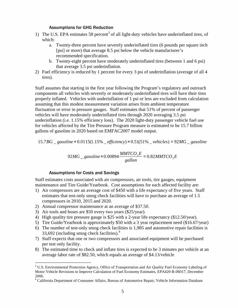
1) The U.S. EPA estimates 58 percent3 of all light-duty vehicles have underinflated tires, of which:
a. Twenty-three percent have severely underinflated tires (6 pounds per square inch [psi] or more) that average 8.5 psi below the vehicle manufacturer’s recommended specification.
b. Twenty-eight percent have moderately underinflated tires (between 1 and 6 psi) that average 3.5 psi underinflation.
2) Fuel efficiency is reduced by 1 percent for every 3 psi of underinflation (average of all 4 tires).
Staff assumes that starting in the first year following the Program’s regulatory and outreach components all vehicles with severely or moderately underinflated tires will have their tires properly inflated. Vehicles with underinflation of 1 psi or less are excluded from calculation assuming that this modest measurement variation arises from ambient temperature fluctuation or error in pressure gauges. Staff estimates that 51% of percent of passenger vehicles will have moderately underinflated tires through 2020 averaging 3.5 psi underinflation (i.e. 1.15% efficiency loss). The 2020 light-duty passenger vehicle fuel use for vehicles affected by the Tire Pressure Program measure is estimated to be 15.7 billion gallons of gasoline in 2020 based on EMFAC2007 model output.
gasolineMGvehiclesefficiencygasolineBG _92)_%51(51.0)_%15.1(0115.0_7.15 =××
EMMTCOgallon
EMMTCOgasolineMG 2
2 82.000894.0_92 =×
Assumptions for Costs and Savings
Staff estimates costs associated with air compressors, air tools, tire gauges, equipment maintenance and Tire Guide/Yearbook. Cost assumptions for each affected facility are: 1) Air compressors are an average cost of $450 with a life expectancy of five years. Staff
estimates that test-only smog check facilities will have to purchase an average of 1.5 compressors in 2010, 2015 and 2020.
2) Annual compressor maintenance at an average of $37.50. 3) Air tools and hoses are $50 every two years ($25/year). 4) High quality tire pressure gauge is $25 with a 2-year life expectancy ($12.50/year). 5) Tire Guide/Yearbook is approximately $50 with a 3 year replacement need ($16.67/year) 6) The number of test-only smog check facilities is 1,985 and automotive repair facilities is
33,692 (including smog check facilities).4 7) Staff expects that one or two compressors and associated equipment will be purchased
per test only facility. 8) The estimated time to check and inflate tires is expected to be 3 minutes per vehicle at an
average labor rate of $82.50, which equals an average of $4.13/vehicle
3 U.S. Environmental Protection Agency, Office of Transportation and Air Quality Fuel Economy Labeling of Motor Vehicle Revisions to Improve Calculation of Fuel Economy Estimates, EPA420-R-06017, December 2006. 4 California Department of Consumer Affairs, Bureau of Automotive Repair, Vehicle Information Database
6
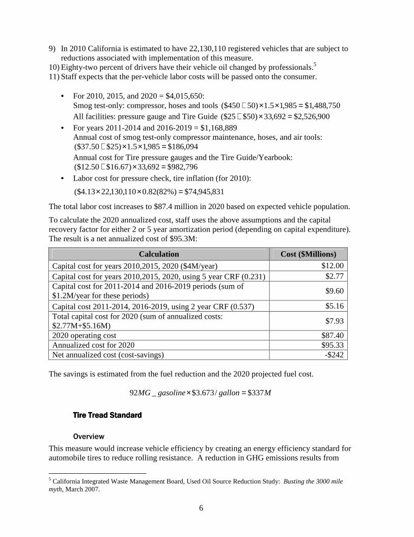
9) In 2010 California is estimated to have 22,130,110 registered vehicles that are subject to reductions associated with implementation of this measure.
10) Eighty-two percent of drivers have their vehicle oil changed by professionals.5 11) Staff expects that the per-vehicle labor costs will be passed onto the consumer.
• For 2010, 2015, and 2020 = $4,015,650: Smog test-only: compressor, hoses and tools 750,488,1$985,15.1)50450($ =××+ All facilities: pressure gauge and Tire Guide 900,526,2$692,33)50$25($ =×+
• For years 2011-2014 and 2016-2019 = $1,168,889 Annual cost of smog test-only compressor maintenance, hoses, and air tools:
094,186$985,15.1)25$50.37($ =××+ Annual cost for Tire pressure gauges and the Tire Guide/Yearbook:
796,982$692,33)67.16$50.12($ =×+
• Labor cost for pressure check, tire inflation (for 2010):
831,945,74$%)82(82.0110,130,2213.4($ =××
The total labor cost increases to $87.4 million in 2020 based on expected vehicle population.
To calculate the 2020 annualized cost, staff uses the above assumptions and the capital recovery factor for either 2 or 5 year amortization period (depending on capital expenditure). The result is a net annualized cost of $95.3M:
Calculation Cost ($Millions)
Capital cost for years 2010,2015, 2020 ($4M/year) $12.00 Capital cost for years 2010,2015, 2020, using 5 year CRF (0.231) $2.77 Capital cost for 2011-2014 and 2016-2019 periods (sum of $1.2M/year for these periods)
$9.60
Capital cost 2011-2014, 2016-2019, using 2 year CRF (0.537) $5.16 Total capital cost for 2020 (sum of annualized costs: $2.77M+$5.16M)
$7.93
2020 operating cost $87.40 Annualized cost for 2020 $95.33 Net annualized cost (cost-savings) -$242
The savings is estimated from the fuel reduction and the 2020 projected fuel cost.
MgallongasolineMG 337$/673.3$_92 =×
Tire TreaTire TreaTire TreaTire Tread Standardd Standardd Standardd Standard
Overview
This measure would increase vehicle efficiency by creating an energy efficiency standard for automobile tires to reduce rolling resistance. A reduction in GHG emissions results from
5 California Integrated Waste Management Board, Used Oil Source Reduction Study: Busting the 3000 mile myth, March 2007.

7
reduced fuel use. Staff estimates that reducing the rolling resistance of tires by 10% results in a 2% increase in fuel efficiency.
Assumptions for GHG Reduction
The tire tread program will provide information to consumers about the availability of tires which are identified as low rolling resistance. Staff uses the following assumptions in calculating the GHG reduction from this measure:
• In 2020, there will be approximately 25 million passenger vehicles in the fleet affected by this measure.
• Approximately 5.5 million vehicles are new and therefore not in the market to purchase new tires.
• New vehicles have low rolling resistance tires as original equipment from the vehicle manufacturer.
• Passenger vehicles affected by this measure drive an average of approximately 12,000 miles per year.
• The fleet average mileage for passenger vehicles affected by this measure is approximately 21 miles per gallon.
• Approximately 15% of tire purchases will be low rolling resistance (i.e. 15% market penetration)
• A 10% reduction in rolling resistance results in a 2% vehicle efficiency increase.
VMTmilesvehiclesvehicles 000,000,100,35000,12000,925,2%15000,500,19 =×=× gallonsgallonsMPGVMT 000,500,33%2571,428,671,121000,000,100,35 =×=÷
EMMTCOMGEMMTCOgallons 22 3.0/00894.0000,500,33 =÷
Assumptions for Costs and Savings
Staff estimates that the there is little, if any, cost differential between tires of varying rolling resistance and therefore assumes no additional cost for choosing low rolling resistance tires. The annual program cost is estimated at $625,000 based on staff experience with programs of similar size and scope. Savings is the result of reduced fuel use.
MgallongasolineMG 123$/673.3$_5.33 =×
Low FrictLow FrictLow FrictLow Friction Engine Oilsion Engine Oilsion Engine Oilsion Engine Oils
Overview
This measure would increase vehicle efficiency by mandating the use of engine oils that meet certain low friction specifications. The American Petroleum Institute has established “energy conserving designation” for certain oils. These specifications would be used as a starting point for the mandated oils under this measure.

8
Assumptions for GHG Reduction
Staff estimates a 2% efficiency increase based on results from research studies.6 Staff estimates the efficiency will be achieved in about 85% of vehicles comprising the light-duty fleet. The 2020 GHG emissions inventory from light-duty vehicles is 160.8MMTCO2E for all fuels.
EMMTCOEMMTCO 22 8.28.160%)85(85.0%)2(02.0 =××
Assumptions for Costs and Savings
Staff estimates approximately $20 per vehicle additional operating and maintenance costs for 26 million vehicles affected by this measure in 2020. Existing oils meeting the low friction criteria are approximately $1/quart more than conventional oil. The $20 incremental cost is based on use of 5 quarts of engine oil at $1 per quart additional for each of 4 oil changes per year. Savings is the result of reduced fuel use of 313 million gallons of gas at $3.673/gallon.
MMGgallon
Mvehiclesmillion
149,1$313/673.3$
520$_2620$
=×=×
Solar Reflective Automotive Paint and Window GlazingSolar Reflective Automotive Paint and Window GlazingSolar Reflective Automotive Paint and Window GlazingSolar Reflective Automotive Paint and Window Glazing
Overview
This measure would increase vehicle efficiency by reducing the engine load for cooling the passenger compartment with air conditioning. The use of solar reflective automotive paints and window glazing reduces heating of the automobile passenger compartment from the sun resulting in reduced air conditioning use. The result is both less frequent air conditioning use by drivers and smaller air conditioners specified by manufacturers for new vehicles.
Assumptions for GHG Reduction
Staff estimates approximately 170 million gallons of gasoline could be saved annually with full implementation of this measure based on results from a National Renewable Energy Laboratory research study and associated modeling results.7 This translates into 1.5 MMTCO2E. This measure is expected to affect 2012 and newer vehicles that are expected to comprise 43% of the 2020 fleet and account for 59% of VMT according to EMFAC20078. The result is a reduction of 0.89 MMTCO2E in 2020.
EMMTCOEMMTCO 22 89.05.1%)59(59.0 −×
6 The Southwest Research Institute (SwRI) conducted a research program that evaluated the effect of engine oil on the fuel economy of gasoline and light-duty diesel engine passenger cars called the Mercedez-Benz M111 Fuel Economy Test—DCED L-54-T-96(http://www.swri.org) 7 National Renewable Energy Laboratory research study “Reduction in Vehicle Temperatures and Fuel Use from Cabin Ventilation, Solar-Reflective Paint, and a New Solar-Reflective Glazing” (Rugh, J.P et al. 2007-01-1194). http://www.nrel.gov/vehiclesandfuels/ancillary_loads/pdfs/40986.pdf 8 The EMissions FACtors (EMFAC) Model is used by ARB to calculate emission rates and population of motor vehicles. Information is available at: http://www.arb.ca.gov/msei/onroad/latest_version.htm

9
Assumptions for Costs and Savings
Staff estimates that the additional cost per vehicle is approximately $250 for complying with this regulation. This includes $10-50/vehicle additional cost for solar reflective paint and $150-225/vehicle additional cost for window glazing. The annualized cost assumes a 14-year CRF (0.101) resulting in approximately $26 per vehicle. It is expected that 14 million vehicles will be affected by this measure resulting in total annualized capital cost of approximately $360M. Savings is the result of reduced fuel use. Reduced fuel of about 99 million gallons results in a $365M savings annually
Measure TMeasure TMeasure TMeasure T----4444————Ship Electrification at Ports (Adopted Regulation)Ship Electrification at Ports (Adopted Regulation)Ship Electrification at Ports (Adopted Regulation)Ship Electrification at Ports (Adopted Regulation)
GHG Reduction Measure
Potential 2020 Reductions MMTCO2E
Annualized Cost
($Millions)
Savings ($Millions)
Net Annualized Cost
($Millions) [Cost-Savings]
Ship Electrification at Ports—Shore Power (Discrete Early Action)
0.2 0 0 0
Overview
This regulation requires ships meeting certain criteria to turn off (cold iron) auxiliary engines at port (hotelling) and acquire power from shore electrification or use another equally effective means of reducing emissions. This measure is motivated primarily by air toxics pollutant reductions but achieves a GHG benefit primarily by shifting electrical generation from high-emitting onboard engines to sources providing electricity to the grid, such as combined-cycle gas turbines.
Assumptions for GHG Reduction
Staff calculated the GHG emission reduction as a ratio of the per megawatt-hour emissions from onboard ship auxiliary power to the shore power emission multiplied by the MWh of electricity supplied to the ship. Staff used 690g/KWh (6.9x10⁻⁷ MMTCO2E/MWh) for auxiliary ship engines. A total estimated 715GWh (715,000MWh) of electricity is used by hotelled ships.9
EMMTCOMWhMWhEMMTCO 227 493.0000,715/109.6 =×× −
EMMTCOMWhValueLineMWhEMMTCO 22
7 312.0000,715)__2020(/1037.4 =×× −
EMMTCOEMMTCOEMMTCO 222 18.0312.0493.0 =−
9 The Initial Statement of Reasons (ISOR) for the Shore Power rule (adopted December 2007) is found at http://www.arb.ca.gov/regact/2007/shorepwr07/tsd.pdf. The ISOR details criteria pollutant and GHG emissions and electricity supplied to hotelled ships.

10
Assumptions for Costs and Savings
The cost and savings associated with this measure are assigned to the diesel risk reduction program and therefore no net cost has been included in the Draft Scoping Plan.
Measure TMeasure TMeasure TMeasure T----5555————Goods Movement Efficiency MeasuresGoods Movement Efficiency MeasuresGoods Movement Efficiency MeasuresGoods Movement Efficiency Measures
GHG Reduction Measure
Potential 2020 Reductions MMTCO2E
Annualized Cost
($Millions)
Savings ($Millions)
Net Annualized Cost
($Millions) [Cost-Savings]
Goods Movement Systemwide Efficiency Measures
3.5 TBD TBD 0
Overview
This measure targets systemwide efficiency improvements in goods movement to achieve GHG reductions from reduced diesel combustion. Staff is developing strategies to achieve the 3.5 MMTCO2E target. The 3.5 MMTCO2E target represents about a 22% reduction from the 2020 projected goods movement inventory.
Assumptions for GHG Reduction
A target of 3.5 MMTCO2E is established in the Draft Scoping Plan. For the purposes of this analysis, staff estimates the targeted reduction will result from reduced diesel combustion from efficiency (90%) and electrification of equipment currently fueled by diesel (10%). However, because this measure is expected to provide flexibility to the industry in determining the emission reduction approaches that work best for them, the proportion of emission reductions from efficiency improvements and electrification may be different than estimated here. The reduction target is the net of GHG reductions from reduced diesel use plus the increases emission from electrification.
Additional assumptions used are as follows: ▪ All fuel used by engines under measure is diesel fuel ▪ Diesel fuel density of 7 lbs. per gallon ▪ Diesel GHG emissions of 10.4 kg CO2E per gallon diesel fuel For conversion from diesel engine to grid power ▪ Grid power emission factor of 437 g CO2E/kWh ▪ Average diesel engine brake specific fuel consumption value (BSFC) of 250 grams
diesel/kWh for the diesel engines covered. Available BSFC data for a sampling of marine, locomotive, and TRU engines ranged from about 200 to 250 g diesel/kWh. Upper end of range (250 g/kWh) used to account for transient operation with lower fuel consumption (higher BSFC).
▪ CO2 emission factor of 790 g/kWh for all engines covered under the measure (estimated using 250 g fuel /kWh BSFC and 10.4 kg CO2E/gallon)
11
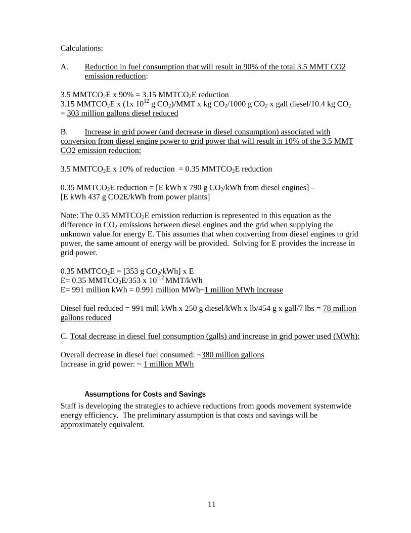
Calculations: A. Reduction in fuel consumption that will result in 90% of the total 3.5 MMT CO2
emission reduction: 3.5 MMTCO2E x 90% = 3.15 MMTCO2E reduction 3.15 MMTCO2E x (1x 1012 g CO2)/MMT x kg CO2/1000 g CO2 x gall diesel/10.4 kg CO2 = 303 million gallons diesel reduced B. Increase in grid power (and decrease in diesel consumption) associated with conversion from diesel engine power to grid power that will result in 10% of the 3.5 MMT CO2 emission reduction: 3.5 MMTCO2E x 10% of reduction = 0.35 MMTCO2E reduction 0.35 MMTCO2E reduction = [E kWh x 790 g CO2/kWh from diesel engines] – [E kWh 437 g CO2E/kWh from power plants] Note: The 0.35 MMTCO2E emission reduction is represented in this equation as the difference in CO2 emissions between diesel engines and the grid when supplying the unknown value for energy E. This assumes that when converting from diesel engines to grid power, the same amount of energy will be provided. Solving for E provides the increase in grid power. 0.35 MMTCO2E = [353 g CO2/kWh] x E E= 0.35 MMTCO2E/353 x 10-12 MMT/kWh E= 991 million kWh = 0.991 million MWh~1 million MWh increase Diesel fuel reduced = 991 mill kWh x 250 g diesel/kWh x lb/454 g x gall/7 lbs = 78 million gallons reduced C. Total decrease in diesel fuel consumption (galls) and increase in grid power used (MWh): Overall decrease in diesel fuel consumed: ~380 million gallons Increase in grid power: ~ 1 million MWh
Assumptions for Costs and Savings
Staff is developing the strategies to achieve reductions from goods movement systemwide energy efficiency. The preliminary assumption is that costs and savings will be approximately equivalent.

12
Measure TMeasure TMeasure TMeasure T----6666————Heavy Duty Vehicle GHG Emission Reduction from Heavy Duty Vehicle GHG Emission Reduction from Heavy Duty Vehicle GHG Emission Reduction from Heavy Duty Vehicle GHG Emission Reduction from AerodynamicAerodynamicAerodynamicAerodynamic Efficiency Efficiency Efficiency Efficiency
GHG Reduction Measure
Potential 2020 Reductions MMTCO2E
Annualized Cost
($Millions)
Savings ($Millions)
Net Annualized Cost
($Millions) [Cost-Savings]
Heavy-Duty Vehicle GHG Emission Reduction from Aerodynamic Efficiency
1.4* 1,136 496* 640*
*This measure would result in 13.6 MMTCO2E outside of California that is not accounted for in this plan. The net annualized cost of this measure incorporates the total cost of the equipment associated with nationwide benefits. The savings, however, only account for the fuel savings that occurs within California associated with the estimated 1.4 MMTCO2E statewide GHG reduction.
Overview
This measure would increase heavy-duty vehicle (long-haul trucks) aerodynamic efficiency by requiring installation of best available technology and/or ARB approved technology to reduce aerodynamic drag and rolling resistance.
Assumptions for GHG Reduction
Staff estimates the 2020 GHG reduction is approximately 15 MMTCO2E nationwide of which 1.4 MMTCO2E (9%) is estimated to occur within California. This reduction is derived from an estimated fuel efficiency improvement of 7% with approximately 1.5% and 5.5% increased efficiency resulting from improvements to the tractor and trailers, respectively. A baseline fuel efficiency of 6 miles per gallon (MPG) is estimated to calculate the benefit from efficiency improvements resulting in an improved mileage of 6.4 MPG (6 MPG X 7% = 6.4 MPG). The 2020 California VMT for heavy-heavy duty diesel trucks (from EMFAC2007) is 17,411,000,000 miles annually of which 2/3 is estimated to derive from trucks affected by this measure (i.e. 11,607,000,000 miles).
gallonsgallonsgallonmiles
miles000,415,135%7000,500,934,1
6
000,000,607,11 =×=
EMMTCOgallonmillionEMMTCO
gallons2
2
4.1_/0104.0
000,415,135 =
Assumptions for Costs and Savings
The incremental costs include for tractors included purchase of tires ($100/tire incremental), and for trailers includes side skirts ($1700), front gap fairing ($800), tires ($100/tire incremental) and installation ($800). An industry average 2.5 trailers per tractor is used to estimate the total cost. The sum of truck retrofit ($1000) plus trailer retrofit ($4100 x 2.5 = $10,250) is $11,250. Staff rounded this to $12,000 for calculation of total cost.
13
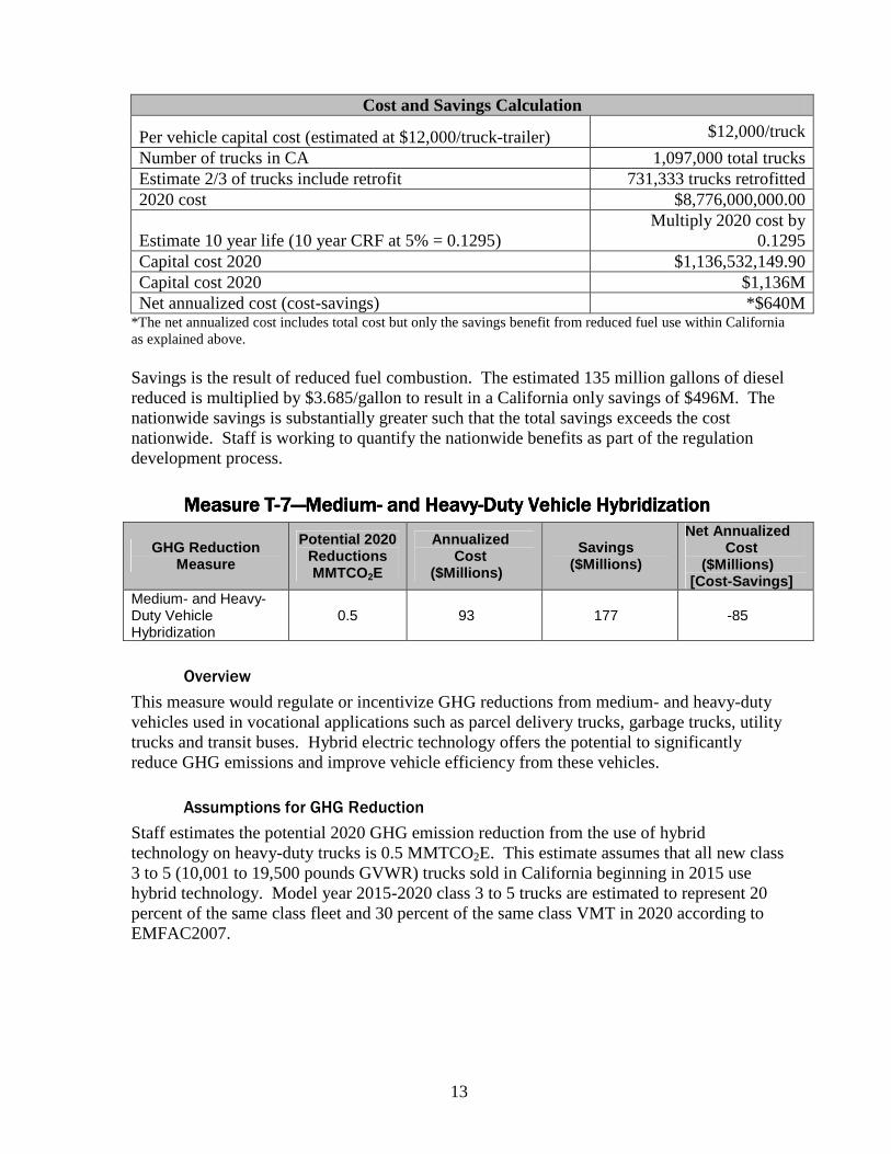
Cost and Savings Calculation
Per vehicle capital cost (estimated at $12,000/truck-trailer) $12,000/truck
Number of trucks in CA 1,097,000 total trucks Estimate 2/3 of trucks include retrofit 731,333 trucks retrofitted 2020 cost $8,776,000,000.00
Estimate 10 year life (10 year CRF at 5% = 0.1295) Multiply 2020 cost by
0.1295 Capital cost 2020 $1,136,532,149.90 Capital cost 2020 $1,136M Net annualized cost (cost-savings) *$640M
*The net annualized cost includes total cost but only the savings benefit from reduced fuel use within California as explained above. Savings is the result of reduced fuel combustion. The estimated 135 million gallons of diesel reduced is multiplied by $3.685/gallon to result in a California only savings of $496M. The nationwide savings is substantially greater such that the total savings exceeds the cost nationwide. Staff is working to quantify the nationwide benefits as part of the regulation development process.
Measure TMeasure TMeasure TMeasure T----7777————MediumMediumMediumMedium---- and Heavy and Heavy and Heavy and Heavy----Duty Vehicle HybridizationDuty Vehicle HybridizationDuty Vehicle HybridizationDuty Vehicle Hybridization
GHG Reduction Measure
Potential 2020 Reductions MMTCO2E
Annualized Cost
($Millions)
Savings ($Millions)
Net Annualized Cost
($Millions) [Cost-Savings]
Medium- and Heavy-Duty Vehicle Hybridization
0.5 93 177 -85
Overview
This measure would regulate or incentivize GHG reductions from medium- and heavy-duty vehicles used in vocational applications such as parcel delivery trucks, garbage trucks, utility trucks and transit buses. Hybrid electric technology offers the potential to significantly reduce GHG emissions and improve vehicle efficiency from these vehicles.
Assumptions for GHG Reduction
Staff estimates the potential 2020 GHG emission reduction from the use of hybrid technology on heavy-duty trucks is 0.5 MMTCO2E. This estimate assumes that all new class 3 to 5 (10,001 to 19,500 pounds GVWR) trucks sold in California beginning in 2015 use hybrid technology. Model year 2015-2020 class 3 to 5 trucks are estimated to represent 20 percent of the same class fleet and 30 percent of the same class VMT in 2020 according to EMFAC2007.

14
From EMFAC2007 CY 2020 (MY 2015-2020)
CY 2020 (ALL MYs)
Assumptions
Vehicles (10,001 to 19,500 lbs)
53,421 273,739
Daily Vehicle Miles (10,001 to 19,500 lbs)
3,694,200 12,166,000
GHGs Reduced in 2020 0.5 MMTCO2E 1.7 MMTCO2E
• Fuel economy improvement: 26%
• Base truck fuel economy: ~7 mpg
gallonsyeardaysdaygallonsgallonmiles
daymiles383,610,47%26/347/742,527
7
/200,694,3 =××= 10
EMMTCOgallonmillionEMMTCO
gallons2
2
5.0_/0104.0
383,610,47 =
Assumptions for Costs and Savings
Base Diesel Truck
Parcel Hybrid Truck
Assumptions
Cost ($) $40,000 $70,000
Cost of the base truck is from a truck dealership. Incremental cost is from a hybrid builder: $30,000 (75% above cost of base truck) for pre-production parcel trucks. ($10,000, or 25% above cost of base truck for production volume of 10,000 trucks or more)
Life of the vehicle (years)
10 10 Source: Parcel delivery truck fleet operator
Maintenance Cost Unknown Unknown
Being pre-production vehicles, the parcel fleet operator has not realized maintenance savings because of problems in software, transmission, parking brake, etc.
Assumed maintenance costs: ($/mile)
$0.16 $0.20
Hybrid truck maintenance cost is assumed to be about 4% lower than base truck for conventional maintenance, but 10% greater when a one-time battery replacement cost of $5000 to $8000 at 22,000 miles/year is included.
10 The VMT output for EMFAC2007 is in units of miles/day for weekday mileage. Annual miles are calculated using a factor of 347 to account for reduced weekend and holiday mileage.

15
Cost and Savings Calculation Number of vehicles 2015-2020 53,421 Per vehicle capital cost $10,000 Capital cost 2015-2020 $534,210,000 10-year CRF at 5% discount rate 0.1295 0.1295 Capital cost 2020 CRF X capital cost $69,180,195 Operating cost $0.20/mile Annual miles 22,000 Operating cost per vehicle $440/year Operating cost 2020 23505240 Operating cost 2020 23.51 Total cost 2020 $92.69M Total fuel reduced 48 million gallons diesel 2020 diesel cost $3.685 Savings from reduced fuel use $177M Net annualized cost (cost-savings) -$85M
Measure TMeasure TMeasure TMeasure T----8888————HeavyHeavyHeavyHeavy----Duty Engine EfficiencyDuty Engine EfficiencyDuty Engine EfficiencyDuty Engine Efficiency
GHG Reduction Measure
Potential 2020 Reductions MMTCO2E
Annualized Cost
($Millions)
Savings ($Millions)
Net Annualized Cost
($Millions) [Cost-Savings]
Heavy-Duty Engine Efficiency
0.6 26 213 -187
Overview
This measure would require the adoption of a regulation and/or incentive program to take advantage of both emerging and current technology to increase the efficiency of heavy-duty engines.
Assumptions for GHG Reduction
The GHG benefits are calculated assuming: • Heavy Heavy-Duty Diesels (HHDD): benefit from all engine efficiency improvement
strategies (18%) • Medium Heavy-Duty Diesels (MHDD): benefit from half of the engine efficiency
improvement strategies (9%) • Both MHDD and HHDD GHG benefits:
o The scenario assumes that engine efficiency improvements are implemented beginning in CY 2016.
o Therefore, in 2020, the affected model years are 2016 to 2020. • Implementation of the Truck and Bus Rule will affect the turn over of the heavy-duty
fleet. o The Truck and Bus Rule requires 70% of the fleet to be turned over by 2015
and 90% by 2020. Therefore, in 2020, the total number of affected vehicles, i.e., MYs 2016 to 2020, is equal to 20% of the total population in 2020

16
From EMFAC2007 Medium Heavy
Duty Diesel Heavy-Heavy Duty Diesel
2020 CA Registered Vehicle Population 235,398 178,262 2020 Total Daily VMT 12,395,000 27,933,000 2020 affected vehicle percentage of same class total 20% 20%
Fuel Economy (mpg) Baseline Fuel Economy 7.2 6.0 Modified Baseline Fuel Efficiency with SmartWay11 7.9 6.2 New Fuel Efficiency for a vehicle with engine efficiency improvement (9% for MHDD and 18% for HHDD)
8.6 7.3
GHG Benefits Fuel Saved (million gallons/day) 0.03 0.14 GHG Reduction 0.1 MMTCO2E 0.5 MMTCO2E Total GHG Reduction 0.6 MMTCO2E Fuel Reduction (2020) 58 million gallons diesel
Assumptions for Costs and Savings
Staff estimates the annualized cost of this measure is $26M. Savings is the result of reduced fuel combustion for an estimated 58 million gallons of diesel in 2020.
MMGgallon 213$58/685.3$ =×
Measure TMeasure TMeasure TMeasure T----9999————Local GLocal GLocal GLocal Government Actions and Regional GHG Targetsovernment Actions and Regional GHG Targetsovernment Actions and Regional GHG Targetsovernment Actions and Regional GHG Targets
GHG Reduction Measure
Potential 2020 Reductions MMTCO2E
Annualized Cost
($Millions)
Savings ($Millions)
Net Annualized Cost
($Millions) [Cost-Savings]
VMT Reduction-Local Government Actions and Targets
2 200 821 -621
Overview
This measure would reduce vehicle miles traveled (VMT) by approximately 2% through land use planning. Staff estimated a 2% reduction based on review of modeling literature.
Assumptions for GHG Reduction
A 2% reduction in VMT results in a 2% reduction in GHG emissions based on the affected portion of the emissions inventory. Passenger vehicles are projected to emit
11 For HHDDs, the modified baseline fuel efficiency (FE) is the weighted average FE and considers 50% of HHDDs to use SmartWay technology (10% improvement) and assumes 75% of the VMT to be at speeds near 60 mph. For MHDDs, the modified baseline weighted average FE considers 25% of the MHDDs to use hybrid technology (40% improvement) and 75% use current technology.

17
160.7 MMTCO2E in 2020 which derives primarily (99.8%) from gasoline combustion. Measures in the Draft Scoping Plan that reduce GHG emissions from reduced fuel consumption and the LCFS12 affecting passenger vehicles include Pavley I and II (measure T-1 reduces GHG emissions by 31.7 MMTCO2E), vehicle efficiency measures (T-3 reduces GHG emissions by 4.8 MMTCO2E). Subtracting the T-1, T-2 (passenger vehicle only portion), and T-3 reductions from the projected inventory results in approximately 115 MMTCO2E net GHG emission for passenger vehicles. A two percent reduction (or 2.3 MMTCO2E) is rounded to 2 MMTCO2E.
EMMTCOEMMTCOEMMTCOEMMTCOEMMTCO 22222 2.1148.4107.317.160 =−−−
EMMTCOEMMTCO 22 3.2%)2(02.02.114 =× Note that the order in which the reductions are calculated changes the resulting expected GHG reduction for this measure. For example, if a 2% reduction in VMT were calculated from the business-as-usual projection of 160.7 MMTCO2E, more than 3 MMTCO2E would result (i.e. 0.02 [2%] x 160.7 MMTCO2E = 3.2 MMTCO2E).
Assumptions for Costs and Savings
Staff conservatively estimates $100/ton of carbon reduced for costs and savings are based upon reduced fuel consumption.
gasolinegallonsmillionEMMTCO
gasolinegallonEMMTCO __223
00894.0
_2
22 =×
milliongallon
gasolinegallonsmillion 821$673.3$
__223 =×
Measure TMeasure TMeasure TMeasure T----10101010————High Speed RailHigh Speed RailHigh Speed RailHigh Speed Rail
GHG Reduction Measure
Potential 2020 Reductions MMTCO2E
Annualized Cost
($Millions)
Savings ($Millions)
Net Annualized Cost
($Millions) [Cost-Savings]
High-Speed Rail 1 0 0 0
Overview
This measure supports implementation of plans to construct and operate a High Speed Rail (HSR) between Northern and Southern California. Development of HSR presents a significant opportunity to reduce GHG emissions by offering more GHG efficient travel options and alternatives to business as usual.
12 Staff estimates the LCFS will reduce passenger vehicle GHG emissions by approximately 10 MMTCO2E in 2020. The passenger vehicle only GHG emissions reduction of 10 MMTCO2E is approximately 2/3 of total LCFS GHG emissions reduction of 16.5 MMTCO2E in 2020.

18
Assumptions for GHG Reduction
Staff analysis of estimated net CO2 emission reductions are based on the HSR operating a Phase 1 system between San Francisco and Anaheim for 2020. Cambridge Energetics forecasts 61.5 million annual passengers (MAP) ridership for this system in 2030. For planning purposes, staff assumes that in 2020 ridership is 40% of this amount, or 24.6 MAP and that operating the HST will require 50% of the energy that it will use in 2030. Staff assumes the ridership will include 17% from air passengers, 76% from motor vehicle passengers, and 7% from conventional rail and induced trips.13
• Air passenger displacement from HSR ridership: Air passengers would number about 4.2 MAP with an associated reduction of 0.33 MMTCO2E based on 350 air miles per passenger trip and 0.5 pounds CO2 per air passenger mile.
• Motor vehicle passenger displacement from HSR ridership: Motor vehicle passengers would number about 18.7 MAP resulting in CO2 emission reduction of 1.28 MMTCO2E based on 225 miles per average motor vehicle trip, 1.5 average occupants per vehicle trip, 22 miles per gallon, and 8.94kgCO2E/gallon of gasoline.
• Riders from other modes would total 1.7 MAP and would displace about 0.04 MMTCO2E, assuming trips in these modes use about 1/3rd the energy per passenger - mile compared to motor vehicle trips.
• The total emissions reduction is the sum of benefits equaling1.65 MMTCO2E per year (0.33 + 1.28 + 0.04).
• A preliminary estimate of total electric energy to operate the HST in Phase 1 in 2030 is 2.3 million megawatt-hours per year. Staff estimates the electricity required in 2020 would be about 50% of this amount, or 1.15 million MWh.
• Using the 2020 emission factor of 4.37x10⁻⁷ MMTCO2E/MWh, the energy to operate the HST would be about 0.5 MMTCO2E. Thus, the net benefit for the Phase 1 HST would be about 1.15 MMTCO2E (1.65 – 0.50).
• Net reduction for HSR is rounded to 1 MMTCO2E.
Assumptions for Costs and Savings
Costs of the measure are the result of existing state policy direction and therefore are not attributed to the AB 32 GHG emissions reduction program.
Transportation Measures Under EvaluationTransportation Measures Under EvaluationTransportation Measures Under EvaluationTransportation Measures Under Evaluation
GHG Reduction Measure
Potential 2020 Reductions MMTCO2E
Annualized Cost
($Millions)
Savings ($Millions)
Net Annualized Cost
($Millions) [Cost-Savings]
Feebates for New Vehicles
4 594 1,642 -1,048∆
Overview
This measure under evaluation would establish a Feebate regulation to reduce passenger vehicle GHG emissions. A Feebate regulation would combine a rebate program for low
13 http://www.cahighspeedrail.ca.gov/images/chsr/20080128135423_R9a_Report.pdf

19
emitting vehicles with a fee program for high emitting vehicles. The regulation would include a fee or rebate of $15-20/gram CO2/mile in relation to a yet undetermined standard.
Assumptions for GHG Reduction
ARB estimates that a fee and rebate schedule of $15-20/gram CO2/mile would result in a fleet mix in 2020 that is about 3% more efficient than what would result from Pavley regulations alone. The GHG reduction is estimated through the fuel savings, using 14.46 billion as the value for gallons of gasoline consumed in 2020 after factoring in the Pavley regulations.
GHG Reduction Calculation BAU gasoline use 17,975 million gallons Gasoline use reduced by Pavley regulations 3,546 million gallons Estimated gasoline consumption after Pavley regulations 14,430 million gallons Additional light-duty fleet efficiency from Feebate regulation 3% Estimated fuel savings from Feebate regulation 447 million gallons Emission factor for 2020 gasoline combustion 0.00894 MMTCO2E/MG GHG reduction from Feebate regulation (EF x fuel use) 4 MMTCO2E
Assumptions for Costs and Savings
Under ARB’s current vision the fee and rebate schedules would be engineered to be revenue neutral after accounting for administrative expenses. That is, there are no net costs associated with program administration. The annualized cost of $594 million is calculated based on the same assumption as Pavley 2, above. Savings is calculated based on reduced fuel consumption of 447 million gallons of fuel, multiplied by $3.673/gallon of gasoline.
Mgasolinegallon
linellons_gasoMillion_ga 642,1$_
673.3$447 =×
20
Electricity and Natural GasElectricity and Natural GasElectricity and Natural GasElectricity and Natural Gas
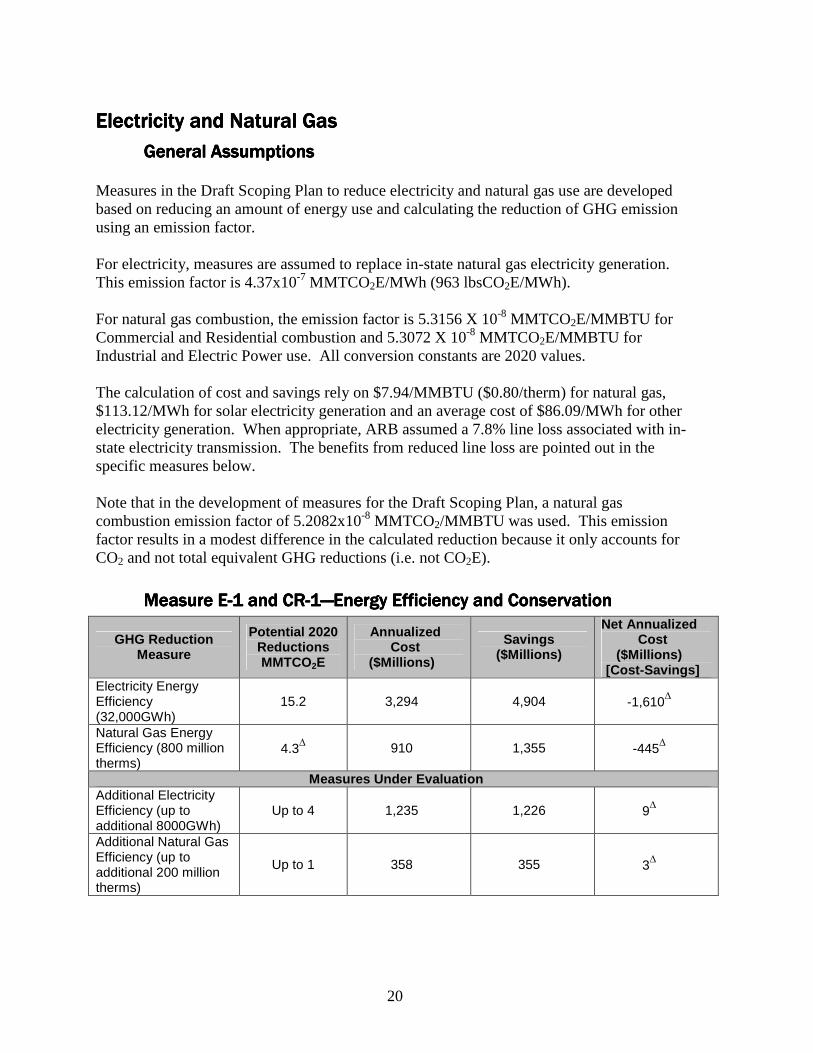
General AssumptioGeneral AssumptioGeneral AssumptioGeneral Assumptionsnsnsns Measures in the Draft Scoping Plan to reduce electricity and natural gas use are developed based on reducing an amount of energy use and calculating the reduction of GHG emission using an emission factor. For electricity, measures are assumed to replace in-state natural gas electricity generation. This emission factor is 4.37x10⁻⁷ MMTCO2E/MWh (963 lbsCO2E/MWh). For natural gas combustion, the emission factor is 5.3156 X 10⁻⁸ MMTCO2E/MMBTU for Commercial and Residential combustion and 5.3072 X 10⁻⁸ MMTCO2E/MMBTU for Industrial and Electric Power use. All conversion constants are 2020 values. The calculation of cost and savings rely on $7.94/MMBTU ($0.80/therm) for natural gas, $113.12/MWh for solar electricity generation and an average cost of $86.09/MWh for other electricity generation. When appropriate, ARB assumed a 7.8% line loss associated with in-state electricity transmission. The benefits from reduced line loss are pointed out in the specific measures below. Note that in the development of measures for the Draft Scoping Plan, a natural gas combustion emission factor of 5.2082x10⁻⁸ MMTCO2/MMBTU was used. This emission factor results in a modest difference in the calculated reduction because it only accounts for CO2 and not total equivalent GHG reductions (i.e. not CO2E).
Measure EMeasure EMeasure EMeasure E----1 and CR1 and CR1 and CR1 and CR----1111————Energy Efficiency and ConservationEnergy Efficiency and ConservationEnergy Efficiency and ConservationEnergy Efficiency and Conservation
GHG Reduction Measure
Potential 2020 Reductions MMTCO2E
Annualized Cost
($Millions)
Savings ($Millions)
Net Annualized Cost
($Millions) [Cost-Savings]
Electricity Energy Efficiency (32,000GWh)
15.2 3,294 4,904 -1,610∆
Natural Gas Energy Efficiency (800 million therms)
4.3∆ 910 1,355 -445∆
Measures Under Evaluation Additional Electricity Efficiency (up to additional 8000GWh)
Up to 4 1,235 1,226 9∆
Additional Natural Gas Efficiency (up to additional 200 million therms)
Up to 1 358 355 3∆

21
Overview
This measure would reduce GHG emissions by increasing statewide energy efficiency for electricity and natural gas beyond current demand projections.
Assumptions for GHG Reduction
For measure E-1, a target of 32,000 GWh reduced demand is assumed. The benefit from reduced line loss (2,707 GWh) is also included.
GWhGWhGWh 707,342707000,32 =+
34,707,000MWh × 4.37×10−7 MMT / MWh =15.2MMTCO2E For measure CR-1 a target of 800 million therms reduced consumption is assumed.
800,000,000therms ×1MMBTU10therm = 80,000,000MMBTU
80,000,000MMBTU × 5.3156×10⁻⁸ MMTCO2E / MMBTU = 4.3MMTCO2E
Likewise, for additional efficiency of 8,000GWh reduced electrical demand and 200 million therms reduced natural gas consumption staff calculates 3.8 MMTCO2E and 1.1 MMTCO2E, respectively.
8,000GWh + 677GWh = 8,677GWh
8,677,000MWh * 4.37×10−7 MMT / MWh = 3.8MMTCO2E
200,000,000therms ×1MMBTU10therm = 20,000,000MMBTU
20,000,000MMBTU × 5.3156×10⁻⁸ MMTCO2E / MMBTU =1.1MMTCO2E
Assumptions for Costs and Savings
Staff estimated the cost and savings from energy efficiency using the Climate Action Team Updated Macroeconomic Analyses Final Report.14 Costs of $217 per ton and savings of $323 per ton of CO2E reduced as derived from the CAT report are used to calculate the net annualized cost for both electricity and natural gas efficiency.
14 The Climate Action Team Updated Macroeconomic Analysis of Climate Strategies for combined electricity and natural gas energy efficiency is found in Exhibit 11 on page 24 of: http://www.climatechange.ca.gov/events/2007-09-14_workshop/final_report/2007-10-15_MACROECONOMIC_ANALYSIS.PDF. Note that the cost and savings are in 2006$ from the CAT report.

22
Measure GHG Reduction
Cost (at $217/MTCO2E) $Millions
Savings (at $323/MTCO2E) $Millions
E-1 15.2 3,294 4,904 CR-1 4.3 910 1,355
Additional Efficiency*
Measure GHG Reduction
Cost (at $325/MTCO2E) $Millions
Savings (at $323/MTCO2E) $Millions
+8000GWh 3.8 1,235 1,226 +200M therms 1.1 358 355
*Costs for additional efficiency are assumed at 50% greater than the cost for the recommended measure. Savings for additional efficiency are assumed to be equivalent to the recommended measure. The net cost and savings per MTCO2E are derived from the average cost and savings in the CAT Macroeconomics report for building and appliance standards and IOU efficiency programs. Staff estimates the cost for additional efficiency under evaluation is 50% greater than the cost for the preliminarily recommended efficiency measures (i.e. $217/MT x 1.5 = $325/MT).
Energy Efficiency Cost and Savings from the CAT-Macroeconomics Update Final Report
Reduction Strategy
GHG Reduction
MMTCO 2E
Cost (2006$)
Savings (2006$)
Cost per MTCO 2E
Savings per MTCO 2E
Building Standards
2.14 $255M $658M $119.16 $307.48
Appliance Standards
4.48 $509M $1,489M $113.62 $332.37
IOU Energy Efficiency Programs
3.66 $987M $1,186M $269.67 $324.04
Additional IOU Energy Efficiency programs
5.60 $1,690M $1,790M $301.79 $319.64
Total 15.88 $3,441M $5,123M $216.69 $322.61
Measure CRMeasure CRMeasure CRMeasure CR----2222————Solar Water HeatingSolar Water HeatingSolar Water HeatingSolar Water Heating
GHG Reduction Measure
Potential 2020 Reductions MMTCO2E
Annualized Cost
($Millions)
Savings ($Millions)
Net Annualized Cost
($Millions) [Cost-Savings]
Solar Water Heating (AB 1470 goal)
0.1 0 0 0∆
Measures Under Evaluation Expanded Solar Water Heating Up to 1 452 160 292

23
Overview
This measure would reduce natural gas use for commercial and residential water heating by installing 200,000 solar water heaters by 2020 per AB 1470 (Huffman). A reduction in GHG emissions of 0.1 MMTCO2E is calculated. Solar heating is an alternative, zero emission, energy source to heat residential water that works with traditional water heating to replace a portion of the natural gas that would normally be burned. The recommended measure would replace an estimated 26 million therms of residential natural gas use each year. ARB is also considering expansion of the measure to reach 1.75 million total installed units by 2020, which would replace approximately 200 million therms of natural gas.
Assumptions for GHG Reduction
Each solar water heater is assumed to reduce annual natural gas use by 130 therms15. In early years of the program, Staff estimates that 5,000 heaters will be installed annually, increasing up to 10,000, 15,000, 25,000 and finally 50,000 installations each year to meet the total 200,000 installed solar water heaters goal.
130therms /heater × 200,000heaters = 26,000,000therms
26,000,000therms ×1MMBTU10therm = 2,600,000MMBTU
2,600,000MMBTU × 5.3156×10⁻⁸ MMTCO2E / MMBTU = 0.14MMTCO2E
For the expanded solar water heating measure under consideration, Staff calculated a GHG reduction based on a total of 1.75 million installed units (i.e. an additional 1,550,000 units).
130therms /heater ×1,550,000heaters = 201,500,000therms
201,500,000therms ×1MMBTU10therm = 20,150,000MMBTU
20,150,000MMBTU × 5.3156×10⁻⁸ MMTCO2E / MMBTU =1.1MMTCO2E
Assumptions for Costs and Savings
Costs of the recommended solar water heating measure are the result of existing state policies (AB 1470) and therefore are not attributed to the AB 32 GHG emissions reduction program. For the expanded solar water heating measure under evaluation, costs are assumed to be $6,500/system for existing homes and $3,000/system for new. Staff assumed a split of 57% new installs and 43% existing building retrofits for cost calculation. Further, Staff estimates a 2% reduction in technology cost annually occurs. Savings of $160 million is the result of reduced natural gas consumption of over 200 million therms at $0.80/therm in 2020.
15 Personal communication, California Center for Sustainable Energy from implementing the CPUC’s pilot project.

24
1.75 Million total units installed (additional 1.55 million to CR-2)
Year Cumulative # SWH Installations (net of CR-2)
Annual Capital Cost* (net of CR-2)
Therms saved/yr (net of CR-2)
2010 0 $0 M M 2011 19,000 $55 M 2 M 2012 68,000 $177 M 9 M 2013 149,000 $293 M 19 M 2014 260,000 $405 M 34 M 2015 404,000 $513 M 52 M 2016 584,000 $676 M 76 M 2017 797,000 $804 M 104 M 2018 1,037,000 $899 M 135 M 2019 1,287,000 $903 M 167 M 2020 1,550,000 $911 M 202 M Total 1,550,000 $5,636 M 202 M *Assume ~20% of cost is covered through incentives & the rest is borne by consumers
Cost and Savings Calculation
Cumulative capital cost $5,636M Estimated Lifetime 20 years CRF (20 year amortization and 5% discount rate) 0.080242587 Annualized capital cost in 2020 (CRF x total capital cost) $452M Natural gas savings 201.5M therms Value of natural gas saved in 2020 (@ $0.80/therm) $160M Net annualized cost (cost-savings) $292M
Measure EMeasure EMeasure EMeasure E----2222————Combined Heat and Power Distributed Electrical Combined Heat and Power Distributed Electrical Combined Heat and Power Distributed Electrical Combined Heat and Power Distributed Electrical GenerationGenerationGenerationGeneration
GHG Reduction Measure
Potential 2020 Reductions MMTCO2E
Annualized Cost
($Millions)
Savings ($Millions)
Net Annualized Cost
($Millions) [Cost-Savings]
Combined Heat and Power 6.7∆ 362 1,673 -1,311
Overview
This measure would encourage the use of efficient combined heat and power co-generation, targeting an increase in installed generation capacity of 4000MW by 2020.
Assumptions for GHG Reduction
For purposes of calculating GHG reductions, Staff estimated the electric generation potential from CHP (of the amount of electricity offset from the grid, based on an assumed 85% capacity factor), the total amount of fuel consumed onsite, and the amount of waste heat generated for useful thermal purposes (which was then used to calculate the amount of fuel not consumed to produce that amount of thermal energy). Staff estimated that 80% of the

25
cogeneration units would be less than 5MW (i.e. small and medium CHP) and 20% greater than 5MW (i.e. large CHP)16. The following table details the assumptions for installations, total electricity generation, amount of natural gas used to make both electricity and heat, the amount of reduced natural gas used in the displaced original heat load, and the net fuel consumption. The total electricity saved includes the benefits of avoided line loss.
Annual
Installations (MW)
Annual MMTherms
For Electricity & Heat
Annual MMTherms Displaced
heating load
Year <5MW >5MW
Total Electricity
Saved (GWh)
<5MW >5MW <5MW >5MW
Net Fuel Consumption (MMTherms)
2009 267 67 2,692 219 48 129 22 116 2010 267 67 5,384 437 97 258 44 232 2011 267 67 8,076 656 145 387 65 349 2012 267 67 10,768 875 194 516 87 465 2013 267 67 13,460 1,094 242 645 109 581 2014 267 67 16,152 1,312 291 774 131 697 2015 267 67 18,844 1,531 339 904 153 814 2016 267 67 21,536 1,750 388 1,033 175 930 2017 267 67 24,228 1,968 436 1,162 196 1,046 2018 267 67 26,920 2,187 484 1,291 218 1,162 2019 267 67 29,612 2,406 533 1,420 240 1,279 2020 267 67 32,304 2,624 581 1,549 262 1,395
*Total 3,200 800 32,304 2,624 581 1,549 262 1,395 4,000 MW total 3,206 1,811
The net GHG reduction is calculated as the difference between the GHG emissions from the grid displaced electricity (32,304GWh including the avoided line loss) and the GHG emissions from natural gas combusted to produce both heat and power onsite. Net Natural gas GHG emission increase:
EMMTCOMMBTUEMMTCOMMBTU 228 41.7/103072.5000,500,139 =×× −
Grid supplied electricity GHG emission decrease:
EMMTCOMWhMMTMWh 27 1.14/1037.4*000,300,32 =× −
Net GHG Reduction:
EMMTCOEMMTCOEMMTCO 222 7.64.71.14 =−
16 California Energy Commission, Draft Consultant Report, Assessment of California CHP Market and Policy Options for Increased Penetration. Prepared by the Electric Power Research Institute. April 2005.
26
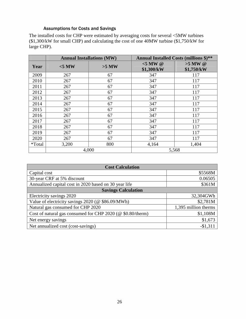
Assumptions for Costs and Savings
The installed costs for CHP were estimated by averaging costs for several <5MW turbines ($1,300/kW for small CHP) and calculating the cost of one 40MW turbine ($1,750/kW for large CHP).
Annual Installations (MW) Annual Installed Costs (millions $)**
Year <5 MW >5 MW <5 MW @ $1,300/kW
>5 MW @ $1,750/kW
2009 267 67 347 117 2010 267 67 347 117 2011 267 67 347 117 2012 267 67 347 117 2013 267 67 347 117 2014 267 67 347 117 2015 267 67 347 117 2016 267 67 347 117 2017 267 67 347 117 2018 267 67 347 117 2019 267 67 347 117 2020 267 67 347 117
*Total 3,200 800 4,164 1,404 4,000 5,568
Cost Calculation Capital cost $5568M 30-year CRF at 5% discount 0.06505 Annualized capital cost in 2020 based on 30 year life $361M
Savings Calculation Electricity savings 2020 32,304GWh Value of electricity savings 2020 (@ $86.09/MWh) $2,781M Natural gas consumed for CHP 2020 1,395 million therms Cost of natural gas consumed for CHP 2020 (@ $0.80/therm) $1,108M Net energy savings $1,673 Net annualized cost (cost-savings) -$1,311

27
Measure EMeasure EMeasure EMeasure E----3333————33% Renewables Portfolio Standard33% Renewables Portfolio Standard33% Renewables Portfolio Standard33% Renewables Portfolio Standard
GHG Reduction Measure
Potential 2020 Reductions MMTCO2E
Annualized Cost
($Millions)
Savings ($Millions)
Net Annualized Cost
($Millions) [Cost-Savings]
33% Renewables Portfolio Standard 21.3∆ 3,671 1,889 1,782∆
Overview
This measure would increase electricity production from eligible renewable power sources to 33% by 2020. A reduction in GHG emissions results from replacing natural gas fired electricity production with zero GHG emitting renewable sources of power.
Assumptions for GHG Reduction
The Renewables Portfolio Standard measure would require 33% of RPS eligible retail electricity sales to be generated from eligible renewable sources. Measures that reduce retails sales of electricity, i.e. efficiency, co-generation, and other distributed generation, are subtracted from the projected demand in 2020 to calculate the amount of generation (in GWh) to meet the 33% renewables standard. The CEC electricity forecast for 2020 projects 308,070 GWh of RPS eligible retails sales. The preliminary recommendation in the Draft Scoping Plan assumes 32,000 GWh of energy efficiency gains, approximately 30,000 GWh of combined heat and power generation, and approximately 4500 GWh of solar distributed generation. There are additional benefits from reduced line loss associated with these measures, which is assumed to be 7.8% statewide.
GWhSolarGWhCHPGWhEEGWhRSGWh 214,236)(845,4)(304,32)(707,34)(070,308 =−−− GWhRPSGWh 951,77)%33(33.0214,236 =×
rget)GWh(RPS_TaRPSCurrentGWhGWh 665,48)_(286,29951,77 =−
EMMTCOMWhMMTMWh 27 25.21/1037.4*000,665,48 =× −
Where RS is 2020 projected retail sales, EE is energy efficiency and conservation plus reduced line loss benefits, CHP is generation from the combined heat and power measure, and Solar is the generation and reduced line loss benefits from the million solar roofs program. Using 4.37x10⁻⁴ MMTCO2E/GWh gives an emissions reduction of 21.3 MMTCO2E. The emissions reduction associated with going from 20% to 33% RPS is necessary for the cost and savings calculation below. Using the approach from above Staff calculates a net GHG emissions reduction for 20-33% RPS of 13.4 MMTCO2E.
GWhRPSGWh 243,47)%20(2.0214,236 =× GWhRPSCurrentGWhGWh 957,17)_(286,29243,47 =−
EMMTCOMWhMMTMWh 27 84.7/1037.4*000,957,17 =× −
EMMTCOEMMTCOEMMTCO 222 4.1384.725.21 =−

28
Assumptions for Costs and Savings
Cost and savings assumptions are derived from Energy and Environmental Economics, Inc.’s (E3) modeling of renewables.17 Staff estimated costs at $274/ MTCO2E and savings at $141/ MTCO2E based on the E3 modeling work with a net cost of $133/MTCO2E for a net GHG reduction going from 20-33% RPS of 13.4 MMTCO2E. Costs for the GHG reduction associated with the existing 20% RPS are the result of existing State policies and therefore are not attributed to the AB 32 GHG emissions reduction program.
13.4MMTCO2E × $274/ MT = $3,671M
13.4MMTCO2E × $141/MT = $1,889M
Measure EMeasure EMeasure EMeasure E----4444————Million Solar RoofsMillion Solar RoofsMillion Solar RoofsMillion Solar Roofs
GHG Reduction Measure
Potential 2020 Reductions MMTCO2E
Annualized Cost
($Millions)
Savings ($Millions)
Net Annualized Cost
($Millions) [Cost-Savings]
Million Solar Roofs 2.1 0 0 0 Measures Under Evaluation
Expanded Million Solar Roofs 1.4∆ $1,348 339 1,009
Overview
This measure follows the direction of Governor Schwarzenegger’s Million Solar Roofs program to install 3000MW of photovoltaic electrical generation in residential and commercial applications by 2017. A measure under evaluation to expand this program by an additional 2000MW (for 5000MW total) by 2020 is included.
Assumptions for GHG Reduction
Staff used a capacity factor for photovoltaic solar power of 17% in calculating the displaced grid electricity from this measure. The benefit from reduced line loss (a constant 7.8%) is also included.
)__(969,251/400,978,2%17/87602000
)__(953,377/600,467,4%17/87603000
losslineavoidedMWhyearMWhyearhoursMW
losslineavoidedMWhyearMWhyearhoursMW
+=××+=××
4,845,553MWh × 4.37×10−7 MMT / MWh = 2.1MMTCO2E
3,230,369MWh × 4.37×10−7 MMT / MWh =1.4MMTCO2E
Assumptions for Costs and Savings
Costs of the E-4 measure are the result of existing state policies and therefore are not attributed to the AB 32 GHG emissions reduction program. For the expanded Million Solar Roofs measure under evaluation Staff assumes an installed cost of $8.40/watt for an additional 2000MW by 2020.
17 Energy and Environmental Economics, Inc. (E3), http://www.ethree.com/GHG/E3_CPUC_GHGResults_13May08%20(2).pdf

29
Cost and Savings Calculation
2000MW @ $8.40/watt $16,800M Estimated Lifetime 20 years CRF (20 year amortization and 5% discount rate) 0.080242587 Annualized capital cost in 2020 (CRF x total capital cost) $1,348M Electricity produced at 17% capacity factor (savings) 2020 3,000,000MWh Value of electricity produced in 2020 (@ $113/MWh) $339M savings Net annualized cost (cost-savings) $1009M
Other Energy Measures Under EvaluationOther Energy Measures Under EvaluationOther Energy Measures Under EvaluationOther Energy Measures Under Evaluation
Coal Emission Reduction StandardCoal Emission Reduction StandardCoal Emission Reduction StandardCoal Emission Reduction Standard
GHG Reduction Measure
Potential 2020 Reductions MMTCO2E
Annualized Cost
($Millions)
Savings ($Millions)
Net Annualized Cost
($Millions) [Cost-Savings]
Coal Emission Reduction Standard
Up to 8 850 0 850
Overview
This measure under evaluation would reduce GHG emissions by replacing coal-produced electricity with less carbon-intensive alternatives. To calculate GHG emissions reduction benefits, Staff assumed 40% of the existing 32,000 GWh of annual coal-produced electricity would be replaced by combined cycle gas turbine (CCGT) power by 2020. A 40% reduction results in 12,800GWh less coal generation in 2020.
Assumptions for GHG Reduction
Staff used 9.88x10⁻⁴ MMTCO2E/GWh for coal generation and 3.22x10⁻⁴ MMTCO2E/GWh for CCGT generation for a net reduction of 6.66x10⁻⁴ MMTCO2E/GWh (i.e. 9.88-3.22=6.66).
6.66×10⁻⁴ MMTCO2E /GWh ×12,800GWh = 8.5MMTCO2E
Assumptions for Costs and Savings
Staff estimated that compliance with this measure under evaluation would cost $100/MTCO2E for a total cost of $850M. This total cost results in a net cost difference between coal and CCGT supplied electricity of $0.066/KWh for an 8.5 MMTCO2E reduction. No savings is assumed.

30
IndustryIndustryIndustryIndustry
Measure IMeasure IMeasure IMeasure I----1: Energy Efficiency and Co1: Energy Efficiency and Co1: Energy Efficiency and Co1: Energy Efficiency and Co----Benefits Audit for Large Benefits Audit for Large Benefits Audit for Large Benefits Audit for Large Industrial SourcesIndustrial SourcesIndustrial SourcesIndustrial Sources
GHG Reduction Measure
Potential 2020 Reductions MMTCO2E
Annualized Cost
($Millions)
Savings ($Millions)
Net Annualized Cost
($Millions) [Cost-Savings]
Energy-Efficiency and Co-Benefits Audit for Large Industrial Sources
TBD TBD TBD TBD
Overview
This recommended measure would require an energy efficiency audit for large stationary GHG emissions sources to identify potential reductions that are cost-effective for GHG, criteria and toxics.
Assumptions for GHG Reduction
TBD
Assumptions for Costs and Savings
TBD
Industrial Measures Under EvaluationIndustrial Measures Under EvaluationIndustrial Measures Under EvaluationIndustrial Measures Under Evaluation
Carbon Intensity Standard for Cement ManufacturersCarbon Intensity Standard for Cement ManufacturersCarbon Intensity Standard for Cement ManufacturersCarbon Intensity Standard for Cement Manufacturers
GHG Reduction Measure
Potential 2020 Reductions MMTCO2E
Annualized Cost
($Millions)
Savings ($Millions)
Net Annualized Cost
($Millions) [Cost-Savings]
Carbon Intensity Standard for California Cement Manufacturers
1.1-2.5 19.4 22.8 -3
Overview
This measure under evaluation sets a standard of 0.8 metric tons of CO2/metric ton of cement as the average carbon intensity factors (CIF) for cement used in California. This standard would apply to imported cement as well as cement manufactured in California. The CIF is defined as metric tons CO2 emitted per metric ton of cement produced. CIF improvements at the cement production level are expected to be met through alternative fuels or energy efficiency measures. There is very little addition of supplementary cementious materials (SCMs) that occur at the manufacturing plants today. Therefore, the focus would be to ensure that lower carbon cement is produced by maximizing the use of alternative fuels and energy efficiency.

31
Assumptions for GHG Reduction
Alternative Fuels The alternative fuel scenario is calculated based on the ARB inventory. The baseline year is 2004 for the cement production and GHG emissions from manufacturers. Staff assumed a 2% annual increase in cement production and imports are 40% of cement consumed in California. The 2004 statewide baseline numbers are as follows:
• Fuel combustion = 4.06 MMTCO2E • Calcination = 5.77 MMTCO2E • Electricity = 0.70 MMTCO2E (based on California Energy Commission emission
factor and the Portland Cement Association external electricity output for 2005) • Total CO2 emissions for California cement plants = 10.53 MMTCO2E • Clinker Production = 11.23 MMT (, 2004) • Cement Production = 11.92 MMT (USGS, 2004)
Based on ARB’s analysis of potential alternative fuel options, we believe a 5 percent reduction in greenhouse gas emissions is feasible and cost-effective. The estimated statewide CIF based on instate cement production is 0.895 metric tons CO2 per metric ton cement. If the 5% reduction were implemented, the CIF for each one would be 0.855. Improved Energy Efficiency The improved energy efficiency is based on fuel and electricity intensity scenarios of 3.0 MBtu per short ton of clinker produced and 109 kWh per ton of cement produced with 2004 and 2005 California cement industry data. Staff estimated an emission reduction of 0.93 MMTCO2E and a 0.055 MTCO2E/MT of cement reduction in the CIF value. When combining the alternative fuel and improved energy efficiency CIF value, the instate CIF value would decrease to below 0.8 MTCO2E/MT cement.
GHG Calculation California Cement Produced 11.92 MMT Current in-state CIF 0.895 CIF with measure under evaluation 0.8 Taking into consideration the 2% growth rate reductions from BAU cement emissions would be:
( ) ( ) ( ) EMMTCOMMTMMT 216 55.137.192.11095.002.192.118.0895.0 =××=××−
Assumptions for Costs and Savings
The ARB 2004 baseline shows that cement manufacturers are using over 3.60 MBtu/ton clinker. Staff believes, through improved energy efficient equipment and using less fuel, that the cement manufacturers would be able to meet a 3.0 MBtu/ton clinker. This number is stated in literature for 4 to 5-stage preheater/precalciner kilns. ARB estimates this will result

32
in an initial capital investment of $220 million dollars with an annual fuel expenditure savings of $22.75 million.
Cost and Savings
Year Capital Costs
($millions)
Cost Savings from Energy Efficiency -
Electricity ($millions)
Cost Savings from Energy Efficiency –
Fuel ($millions)
Cost Increase from Alternative
Fuels ($millions)
2012 220 11.66 17.45 11.46 2013 11.89 17.80 11.69 2014 12.13 18.16 11.93 2015 12.37 18.52 12.16 2016 12.62 18.89 12.41 2017 12.87 19.27 12.66 2018 13.13 19.65 12.91 2019 13.39 20.05 13.17 2020 13.66 20.45 13.43
Cost and Savings Calculation Annualized Capital Expenditure: $202.4 million*0.0802 = $16.23 million (CA cement manufacturers annualized capital cost) $16.23 million + $1.35 million (annual operating cost) = $17.58 million (CA cement manufacturer’s total annual cost) $17.58 million*1.10 (10% of $17.58 million is the capital cost for imported cement) = $19.34 million Annual Fuel Expenditure Savings: $13.66 million + $20.45 million – $13.43 million = $20.68 million $20.68 million*1.10 (10% of $20.68 million is the fuel savings for imported cement) = $22.75 million Net Annual Savings: $3.41 million
Carbon Intensity StanCarbon Intensity StanCarbon Intensity StanCarbon Intensity Standard for Concrete Batch Plantsdard for Concrete Batch Plantsdard for Concrete Batch Plantsdard for Concrete Batch Plants
GHG Reduction Measure
Potential 2020 Reductions MMTCO2E
Annualized Cost
($Millions)
Savings ($Millions)
Net Annualized Cost
($Millions) [Cost-Savings]
Carbon Intensity Standard for Concrete
Batch Plants 2.5-3.5 0 0 0
Overview
This measure under evaluation would require concrete batch plants to have a lower carbon intensity factor (CIF) for cementious material than the CIF required at the cement manufacturing facility. The standard would be set at 0.6 metric ton CO2/metric ton of cementious material used. The standard at the concrete batch plant could be met either by

33
using cement with very low carbon intensity factors, by adding materials such as SCMs to replace cement in the concrete blend, or using a combination of both approaches.
Assumptions for GHG Reduction
Concrete batch plants can double the total amount of CO2 reductions through blending of cement compared to the cement manufacturers. The scenario for the concrete batch plants is to blend SCMs in Portland cement to equal at least 15% or more of blended cement and meet a 0.66 CIF standard by 2012. In 2015, the cement that is used to manufacture concrete must meet a 25% blend of SCMs and comply with a 0.6 CIF standard. The CIF standard for cement used by concrete batch plants in 2012 through 2014 would comply with 0.66 MT CO2/MT cement. By 2015, the CIF for cement would be 0.6 MTCO2/ MT cementious material. The calculation for GHG reductions in 2020 is below. GHG calculation assumptions:
• California Cement Produced: 11.92 MMT • CIF Factor Under Manufacturer Regulations: 0.8 • CIF Under Batch Plant Regulations: 0.6
Taking into consideration the 2% growth rate reductions from BAU cement emissions would be:
( ) ( ) ( ) EMMTCOMMTMMT 216 27.337.192.112.002.192.116.08.0 =××=××−
Assumptions for Costs and Savings
Currently, the cost of a ton of SCMs is approximately the same as the cost of a ton of cement (about $100/ton). Therefore Staff estimates there is no net cost or savings for this measure.
Waste Reduction in Concrete UseWaste Reduction in Concrete UseWaste Reduction in Concrete UseWaste Reduction in Concrete Use
GHG Reduction Measure
Potential 2020 Reductions MMTCO2E
Annualized Cost
($Millions)
Savings ($Millions)
Net Annualized Cost
($Millions) [Cost-Savings]
Waste Reduction in Concrete Use
0.5-1.0 55 83 -28
Overview
This measure under evaluation would set a minimum waste requirement or establish emissions fees on unused returned concrete.
Assumptions for GHG Reduction
ARB estimates that approximately five to eight percent of the concrete that is made in California each year is returned to the plant as waste. Given cement is the main source of GHG emissions in concrete, a reduction opportunity over 1 MMTCO2E exists by 2020.

34
GHG calculation assumptions: • Total Cement: 11.92 MMT • Wasted Cement: (0.08)(11.92)= 0.954 MMT • Current CIF: 0.895 MTCO2/MT cement • 2% Annual Growth Rate
EMMTCOMMT 2
16 17.1895.002.192.1108.0 =×××
Assumptions for Costs and Savings
ARB assumes $100 as an average cost per ton of cement and an added operational cost of $70 per ton of wasted cement to achieve maximum efficiency. This results in a net cost savings of $30/ton of cement and an annual savings of $28 million.
Cost and Savings Calculation Wasted Cement 0.954MMT Net savings per MT ($100-$70=$30) $30 Annual savings $28M
Refinery Energy Efficiency Process ImprovementsRefinery Energy Efficiency Process ImprovementsRefinery Energy Efficiency Process ImprovementsRefinery Energy Efficiency Process Improvements
GHG Reduction Measure
Potential 2020 Reductions MMTCO2E
Annualized Cost
($Millions)
Savings ($Millions)
Net Annualized Cost
($Millions) [Cost-Savings]
Refinery Energy Efficiency Process Improvements
2-5 71 461 -390∆
Overview
This measure under evaluation would reduce GHG emissions from refineries by reducing fossil fuels consumption across a variety of refinery processes including process heaters, boilers, fluid catalytic crackers, hydrogen plants, and flares.

35
Assumptions for GHG Reduction
Measure Description Number of
Units Affected
Estimated Capital
Cost ($million)
Existing Emissions
(MMT CO2E)
Emissions Reduction
(MMT CO2E)
Percent Emissions Reduction
1.Improve Efficiency of Boilers and
Process Heaters
Improve efficiency of half of total
units by 15%
300 of 600 272 14.8 1.0 6.8
2.Install FCC Power
Recovery Turbine
Capture mechanical
work from FCC regenerator flue
gas
3 of 10 21 6.11* 0.47 7.7
3.Improve Catalyst Type
at FCC
Reduce carbon buildup on
catalyst 4 of 10 11
* included above
0.82 13
4.Modernize Hydrogen
Plants
Use pressure swing
adsorption technology
Reduce H2 plant
emissions by 20% overall
387 5.8 1.1 19
5.Increase Gas Recovery
Capacity at Flares
Install additional
compressors in flare systems
Flare systems
at 19 refineries
71 0.67 0.33 50
Totals 762 27.4 3.7 1418 Notes:
1. Improve efficiency of 300 boilers and process heaters from 73 percent to 88 percent (fuel savings)
2. Valero refinery in Houston uses pressure drop of regenerator gas to drive turbine and recover mechanical power to compress regenerator inlet air, saving 22MW of energy otherwise needed for this compression (assume fuel savings)
3. Less carbon buildup on catalyst means less combustion to remove it (fuel savings) 4. Pressure swing adsorption requires 20 percent less energy than amine systems per
cubic foot of hydrogen produced (fuel savings) 5. Measure entails providing adequate gas recovery capacity and best operating
practices (fuel recovery savings)
18 Total refinery GHG emissions are estimated at 35.2 MMT CO2 E. Therefore, overall estimated refinery emissions reductions represent 11 percent of that total.

36
Assumptions for Costs and Savings
Cost and Savings Calculation Capital cost 2020 $762M Capital life 20 years 20-year CRF (@5% discount rate) 0.08024 Annual cost 2020 (Capital cost x CRF) $61M 2020 operational costs $10M total annual cost 2020 $71M Natural gas savings 56,900,000 MMBTU 2020 value of fuel savings (@ $7.94/MMBTU) $452M Operational savings $9M Total savings $461M Net annualized cost (cost-savings) -$390M
Removal of Methane Exemption from Existing Refinery RegulationsRemoval of Methane Exemption from Existing Refinery RegulationsRemoval of Methane Exemption from Existing Refinery RegulationsRemoval of Methane Exemption from Existing Refinery Regulations
GHG Reduction Measure
Potential 2020 Reductions MMTCO2E
Annualized Cost
($Millions)
Savings ($Millions)
Net Annualized Cost
($Millions) [Cost-Savings]
Removal of Methane Exemption from Existing Refinery Regulations
0.01-0.05 5 2.7 2∆
Overview
This measure under evaluation would remove the methane exemptions from the regulations applicable to equipment and sources employed in California’s refineries.
Assumptions for GHG Reduction
ARB relied on the analysis performed by South Coast Air Quality Management District (SCAQMD) for the adoption of their Rule 1173, Control of Volatile Organic Compound Leaks and Releases from Components at Petroleum Facilities and Chemical Plants. ARB staff assumed that exempt hydrocarbons, assumed to be methane, could be reduced by a similar 80 percent if the equipment associated with the processing and piping of the methane-rich streams were subject to the leak detection and repair requirements of the rule. Staff also applied this factor to two refineries located in the San Joaquin Valley Unified Air Pollution Control District. The Bay Area Air Quality Management District rule for leak detection and repair already included methane.
Assumptions for Costs and Savings
ARB staff used the cost estimates provided by the SCAQMD analysis for Rule 1173, updated the labor costs, estimated that an additional five percent of valves, compressors, and connections would be inspected and repaired, and applied these factors to the SCAQMD and SJVAPCD.

37
Cost and Savings Calculation Operational cost in 2020 $5M 2020 Savings $2.7M Net annualized cost (cost-savings) $2M
Oil and Gas Extraction GHG Emission ReductionOil and Gas Extraction GHG Emission ReductionOil and Gas Extraction GHG Emission ReductionOil and Gas Extraction GHG Emission Reduction
GHG Reduction Measure
Potential 2020 Reductions MMTCO2E
Annualized Cost
($Millions)
Savings ($Millions)
Net Annualized Cost
($Millions) [Cost-Savings]
Oil and Gas Extraction GHG Emission Reduction
1-3 107 274 -167∆
Overview
This measure under evaluation would address GHG emissions from the extraction of California’s large oil and gas industry, including on and off-shore sources. Extraction-related GHG emissions come primarily from combustion (95%) and secondarily from fugitive sources. These emissions are produced mainly from the combustion of natural gas in generators, boilers, pumps and other related equipment. This measure would include: repowering, retrofitting, replacing or repairing existing equipment; installing new combined heat and power; electrifying equipment; using monitoring equipment to detect leaks; and possibly employing CO2 injection to enhance oil recovery.
Assumptions for GHG Reduction
Replacement and retrofitting of boilers and steam generators with more efficient ones, as well as replacing internal combustion engine (ICE) pumps with electric motors, achieves an estimated 1.8 MMTCO2E reduction. The remaining 0.2 MMTCO2E reduction comes from a limited amount of changing operating practices while taking compressors off-line; installing compressor rod packing systems; replacing high-bleed pneumatics with low-bleed pneumatics; improved leak detection; and installing electronic flare ignition devices. These estimations will be refined as a more robust emission inventory is developed via an industry-wide survey and the control approaches of the measure identified.

38
Assumptions for Costs and Savings
Cost and Savings Calculation Capital cost $357M Estimated capital lifetime 20 years 20-year Capital Recovery Factor 0.08024 Annualized Capital cost 2020 $28.6M Operating cost in 2020 $23.3M Non-energy cost savings in 2020 $8.8 Electricity use 637,000 MWh Value of electric use in 2020 (@ $86/MWh) $55M Natural gas reduction 33,400,000 MMBTU Value of Natural Gas Savings (@ $7.94/MMBTU) $265M Total 2020 cost $106.9M Total 2020 savings $274M Net annualized cost (cost-savings) -$167M
GHG Leak Reduction from Oil and Gas TransmissionGHG Leak Reduction from Oil and Gas TransmissionGHG Leak Reduction from Oil and Gas TransmissionGHG Leak Reduction from Oil and Gas Transmission
GHG Reduction Measure
Potential 2020 Reductions MMTCO2E
Annualized Cost
($Millions)
Savings ($Millions)
Net Annualized Cost
($Millions) [Cost-Savings]
GHG Leak Reduction from Oil and Gas Transmission
0.5-1.5 19 34.2 -15
Overview
This measure under evaluation addresses emissions from the transmission and distribution of natural gas throughout California. This measure would included: replacing older equipment (flanges, valves and fittings); substituting high bleed with low bleed pneumatic devices; installing vapor recovery devices; using emission monitoring equipment to detect leaks; installing more energy efficient equipment; switching to low carbon fuels to run the equipment; and improving practices for inspection and management.
Assumptions for GHG Reduction
Changing operating practices while taking compressors off-line achieves almost all of the estimated 0.9 MMTCO2E emissions reduction. Replacing just a handful of ICE pumps and compressors with electric motors achieves the remaining 0.1 MMTCO2E emissions reduction. These estimations will be refined as a more robust emission inventory is developed via an industry-wide survey and the control approaches of the measure identified

39
Assumptions for Costs and Savings
Cost and Savings Calculation Capital cost 2015 $28M Lifetime 5 years 5-year Capital Recovery Factor 0.2310 Annualized capital cost 2020 $6.6M Electricity cost 138,000 MWh Value of electricity cost in 2020 (@$86/MWh) $12M Natural gas reduction 4,130,000 MMBTU Value of natural gas savings (@ $7.94/MMBTU) $33M Operating cost 2020 $0.54M Non-energy cost savings in 2020 $1.2M Total 2020 cost $19.0M Total 2020 savings $34.2M Net annualized cost (cost-savings) -$15
Industrial Boiler EfficiencyIndustrial Boiler EfficiencyIndustrial Boiler EfficiencyIndustrial Boiler Efficiency
GHG Reduction Measure
Potential 2020 Reductions MMTCO2E
Annualized Cost
($Millions)
Savings ($Millions)
Net Annualized Cost
($Millions) [Cost-Savings]
Industrial Boiler Efficiency
0.5-1.5 22.9 150 -127
Overview
This measure under evaluation would require one or more of the following: annual tuning of all boilers, the installation of an oxygen trim system, and/or a non-condensing economizer to maximize boiler efficiency. A source could also replace an existing boiler with a new one that is equipped with these systems.
Assumptions for GHG Reduction
Assumptions: • Estimated annual emissions based on draft Greenhouse Gas Inventory Forecast
Estimates (February 6, 2008) 2020 projected emissions from natural gas: 24.19 MMTCO2E
• Boiler efficiency measure applies to approximately 80% of the universe due to this natural gas usage
• Boiler Efficiency Measure accomplishes a 5% reduction in GHG emissions
(0.80)(24.19 MMTCO2E)(0.05) = 1.0 MMTCO2E reduction annually The Boiler Efficiency Measure requires the efficiency improvements summarized in the table below. Costs were estimated by determining the cost of each requirement and the approximate number of boilers that would need each type of the two retrofits or tuning.

40
Summary of Measure Requirements Applicability Requirement All permitted boilers Annual tuning Boilers rated at or over 10 MMBtu/hr Retrofit with an oxygen trim system including
parallel positioning and VFD Boilers rated at or over 50 MMBtu/hr Retrofit with a non-condensing economizer
Assumptions for Costs and Savings
• Total Capital Cost ($90,390,000) o The capital cost is derived from the cost of purchasing and installing
equipment retrofits required by the measure multiplied by the approximate total number of installations. The total number of installations was estimated using engineering judgment, data from ARB’s CEIDARS database, air district databases, and from information supplied by an industry sales representative and representatives of a consulting firm that administers a commercial and industrial boiler efficiency program.
• Annual Tuning requirement o Capital cost = $0.
• Retrofit of 10 MMBtu/hr boilers with oxygen trim, parallel positioning, VFD • Equipment costs for retrofit assuming 600 boilers rated at or over 10 MMBtu/hr with
oxygen trim, parallel positioning, and VFD ($96,000 per unit) = $57,600,000 • Note: Assumed 60% (600) of the 1000 boilers in CEIDARS inventory are not
already equipped with oxygen trim, parallel positioning, and VFD and need the retrofit.
• Capital costs for retrofit of 105 boilers rated at or over 50 MMBtu/hr with a non-condensing economizer ($200,000 per unit) = $21,000,000
• Assumed 60% (105) of the 175 boilers in the State are not already equipped with a non-condensing economizer and need the retrofit. South Coast database shows there are 70 boilers in the District over 50 MMBtu/hr.
• Assuming South Coast has 40 percent of the inventory in the State, the total number of boilers over 50 MMBtu/hr in California is 70/0.4 = 175 boilers.
• Capital costs: $78,600,000 • Total installation costs (15 percent of capital costs) = $11,790,000 • Total capital and installation costs for boiler retrofits = $90,390,000 • Annual operating cost ($15,610,000) • Annual maintenance costs for boiler retrofits (assumed to be 10 percent of capital
costs) = $7,860,000 • Annual tuning costs for 3100 boilers ($2500 per unit) = $7,750,000 • Note: all the costs for the tuning requirement are considered to be an annual
maintenance cost. The 2004 CEIDARS NOx inventory showed approximately 3100 permitted natural gas boilers.
• Total annual operating costs (annual maintenance costs and annual tuning costs) = $15,610,000
• Lifetime Expenditures 2016 through 2020 ($168,440,000) • $90,390,000 + (5 years)($15,610,000) = $168,440,000

41
• Cost Savings ($149,640,000) • (There will also be an unknown electricity savings from the VFD.)
o 1 MMTCO2E)(106 metric ton/MMT)/(0.05306 metric tons CO2/MMBtu) = 18,846,588 MMBtu natural gas annual savings
• Annual fuel cost savings ($7.94/MMBtu)(18,846,588 MMBtu) = $149,641,908 • Lifetime Cost Savings 2016 through 2020 • (5 years)($149,641,908) = $748,209,543
Summary Cost and Savings Calculation
Total capital cost $90.4M Operating cost 2020 $16M Estimated capital life 20 years 20-year CRF 0.08024 Annualized capital cost (capital x CRF) $7.25M Total cost in 2020 $22.86M Natural gas savings 18,846,588 MMBTU Value of Natural Gas Savings in 2020 (@ $7.94/MMBTU) $149.7M Net annualized cost (cost-savings) -$127M
Stationary Internal Combustion Engine ElectrificationStationary Internal Combustion Engine ElectrificationStationary Internal Combustion Engine ElectrificationStationary Internal Combustion Engine Electrification
GHG Reduction Measure
Potential 2020 Reductions MMTCO2E
Annualized Cost
($Millions)
Savings ($Millions)
Net Annualized Cost
($Millions) [Cost-Savings]
Stationary Internal Combustion Engine Electrification
0.1-0.5∆ 17.9 25 -7.1∆
Overview
This measure under evaluation would affect owners and operators of engines in industrial and commercial operations rates at over 50 hp and used as primary power sources (“prime” engines). This measure would not affect internal combustion (IC) engines used for emergency power generation. This measure would include the replacement of IC engines with electric motors (electrification).
Assumptions for GHG Reduction
In the Draft Scoping Plan ARB estimated the GHG emission reduction potential as approximately 0.1 to 1.0 MMTCO2E. As ARB continued to evaluate this measure, it became apparent the high end of the range – 1 MMT, was unrealistic. Such a large reduction would require electrifying over two-thirds of the engines in this category by 2020. This level is not achievable due to both logistical difficulties (access to electrical service and/or required duty cycles) and high cost for engines that are not operated a high percentage of the time. To reflect this, ARB believes a more realistic range of potential reductions is 0.1 to 0.5.

42
Assumptions for Costs and Savings
Cost and Savings Calculation Total capital cost $50.7M Operating cost 2020 $14M Estimated capital life 20 years 20-year CRF (@ 5% discount rate) 0.8024 Annualized capital cost (capital x CRF) $4.1M Total 2020 cost $17.9M Natural Gas Savings 7,670,600 MMBTU Value of Natural Gas Savings in 2020 (@ $7.94/MMBTU 60.92 Diesel Savings in 2020 11.4 million gallons Value of Diesel Savings 2020 (@ $3.685/gallon) $41.9M Increased electricity use in 2020 904,443 MWh Cost of increased electricity (@ $86/MWh) $77.9M Net savings in fuel 25.04 Net annualized cost (cost-savings) -$13M
Glass Plant Energy EfficiencyGlass Plant Energy EfficiencyGlass Plant Energy EfficiencyGlass Plant Energy Efficiency————Equipment Efficiency and Use of Equipment Efficiency and Use of Equipment Efficiency and Use of Equipment Efficiency and Use of Recycled MaterialsRecycled MaterialsRecycled MaterialsRecycled Materials
GHG Reduction Measure
Potential 2020 Reductions MMTCO2E
Annualized Cost
($Millions)
Savings ($Millions)
Net Annualized Cost
($Millions) [Cost-Savings]
Glass Manufacturing Energy Efficiency
0.1-0.2 36.9 23.6 13∆
Overview
This measure under evaluation would increase the requirement for recycled glass (cullet) content and would require facilities to use the best technology to reduce GHG emissions or adopt energy efficient operation and maintenance procedures for manufacturing glass.
Assumptions for GHG Reduction
The GHG emissions reduction was based on the industry’s increase in cullet use of 10% or more and the use of other potential energy efficiency measures which would result in 5 to 10% energy savings.

43
Assumptions for Costs and Savings
Cost and Savings Calculation Total capital cost $15M Estimated capital life 10 years 10-year CRF 0.1295 Annualized capital cost (capital x CRF) $1.94M 2020 operating cost $35M 2020 total annualized cost $36.94M Natural gas savings 281700 MMBTU Value of natural gas savings (at $7.94/MMBTU) $2.24M Electricity savings 5979 MWh Value of electricity savings (at $86/MWh) $0.5M Operational cost saving as a result of material $20.8M Total savings $23.6M Net annualized cost (cost-savings) $13M
OffOffOffOff----Road EquipmentRoad EquipmentRoad EquipmentRoad Equipment
GHG Reduction Measure
Potential 2020 Reductions MMTCO2E
Annualized Cost
($Millions)
Savings ($Millions)
Net Annualized Cost
($Millions) [Cost-Savings]
Off-road Equipment Up to 0.5 TBD TBD TBD
Overview
This measure targets a number of efficiency improvements in offroad equipment including solar-reflective paint and window glazing, reduced idling emissions, equipment electrification, and low friction engine oil. Staff is evaluating the potential GHG reductions and cost and savings from this measure.
Assumptions for GHG Reduction
TBD
Assumptions for Costs and Savings
TBD

44
Recycling and WasteRecycling and WasteRecycling and WasteRecycling and Waste
Landfill Methane CaptureLandfill Methane CaptureLandfill Methane CaptureLandfill Methane Capture
GHG Reduction Measure
Potential 2020 Reductions MMTCO2E
Annualized Cost
($Millions)
Savings ($Millions)
Net Annualized Cost
($Millions) [Cost-Savings]
Landfill Methane Capture (Discrete Early Action)
1 5219 0 52
Overview
This measure would reduce methane emissions from municipal solid waste landfills by requiring owners and operators to install gas collection and control systems at smaller and other uncontrolled landfills. Additionally, all affected landfills will be required to satisfy enhanced methane monitoring requirements to ensure that their gas collection and control system is operating optimally and that fugitive emissions are minimized.
Assumptions for GHG Reduction
Staff estimates 0.8 MMTCO2E GHG emissions reduction from the approximately 53 landfills having greater than 450,000 tons of waste-in-place that may generate sufficient gas to support the installation of a gas collection and control system with a flare. Staff estimated an additional 0.2 MMTCO2E GHG emissions reduction from enhanced monitoring requirements to ensure that the landfill’s gas collection and control system is operating optimally and that fugitive emissions are minimized. The total estimated reduction is 0.8+0.2 = 1 MMTCO2E.
Assumptions for Costs and Savings
Staff estimated a capital cost of $3,438,000 and annual operating cost of $706,397 for the aforementioned 53 facilities. The lifetime of the gas collection and control systems is estimated at 15 years. The total estimated cost is approximately $1M per facility in 2020. Total industry costs, included those for landfills with existing gas collection and control systems, will be estimated in the staff report for the landfill methane control measure. The costs and emission reduction estimates presented here are preliminary estimates.
19 In reviewing costs for the Landfill Methane Capture measure staff corrected the cost value in this documentation supplement. The cost value published in the Draft Scoping Plan Appendix of $1M is per landfill and not total.

45
Cost Calculation Capital cost $3,438,000 Capital life 20 years 20 year CRF 0.08024 Annualized capital cost $275,874 2020 Operating cost $706,397 Total per facility cost $982,271 Total cost (for 53 facilities) $52M Savings $0 Net annualized cost (cost-savings) $52M
High Global Warming PotentialHigh Global Warming PotentialHigh Global Warming PotentialHigh Global Warming Potential
Measure HMeasure HMeasure HMeasure H----1: Motor Vehicle Air Conditi1: Motor Vehicle Air Conditi1: Motor Vehicle Air Conditi1: Motor Vehicle Air Conditioning Systems: Reduction of oning Systems: Reduction of oning Systems: Reduction of oning Systems: Reduction of Refrigerant Emissions from NonRefrigerant Emissions from NonRefrigerant Emissions from NonRefrigerant Emissions from Non----Professional Servicing (Discrete Professional Servicing (Discrete Professional Servicing (Discrete Professional Servicing (Discrete Early Action)Early Action)Early Action)Early Action)
GHG Reduction Measure
Potential 2020 Reductions MMTCO2E
Annualized Cost
($Millions)
Savings ($Millions)
Net Annualized Cost
($Millions) [Cost-Savings]
Sales Restriction on Containers of Refrigerant
0.5 60 0 60∆
Alternative Proposal 0.25 3 0 3
Overview
This measure reduces GHG emissions from the non-professional servicing of motor vehicle air conditioning systems by do-it-yourself individuals. The basic structure and approach of this measure is essentially the same as that originally proposed in the Early Action Plan. There are two proposals currently undergoing consideration: a sales restriction (can ban) and an alternative approach. The alternative approach would include: 1) the installation of a self-sealing dispensing valve on all small containers of refrigerant, 2) the implementation of a mandatory container recycling and refrigerant recovery program, 3) improved labeling on all containers, and 4) the implementation of a consumer education program. Since this is a Discrete Early Action, the proposed regulation would become enforceable on January 1, 2010. The table above includes two rows, corresponding to the two approaches that were considered by Staff. The Draft Scoping Plan Appendix C includes only the original estimate associated with the Staff recommendation, the Alternative Proposal. The numbers above are refinements based on the most recent information emerging from the public process.
Assumptions for GHG Reduction
The total annual emission reduction from the “Can Ban” amounts to approximately 0.47 MMTCO2E and is principally due to the prohibition of sales and the significantly reduced do-it-yourself practice in California.

46
The alternative approach is estimated to achieve a reduction of approximately 0.25 MMTCO2E in 2020 resulting from the recovery of the unused refrigerant in the containers and an increased consumer awareness of an optimum charging techniques arising from the improved labeling and the education program.
Assumptions for Costs and Savings
Under the “Can Ban,” there would be no costs or charges imposed on the small can industry to comply with the ban, but there would be complete loss of revenues which would amount to $25 million in California. Under the small can ban, consumer costs would be affected by the difference between the cost of professional repairs and the cost of DIY recharges. The cost to consumers would increase by $74 million annually. The industry has estimated that the installation of self-sealing valves and the implementation of the recycling program would result in a cost increase of one dollar per container. At 1.6 million cans per year the increased consumer cost is $1.6 million. Assuming a 95% can return rate and a $10 deposit per can, the 5% of unclaimed deposits amounts to $0.8 million per year and will be an additional cost to the consumers. Total increased cost to the consumer is thus ~$3 million per year.
Measure HMeasure HMeasure HMeasure H----2: SF2: SF2: SF2: SF6666 Limits in Non Limits in Non Limits in Non Limits in Non----Utility and NonUtility and NonUtility and NonUtility and Non----Semiconductor Semiconductor Semiconductor Semiconductor Applications (Discrete Early Action)Applications (Discrete Early Action)Applications (Discrete Early Action)Applications (Discrete Early Action)
GHG Reduction Measure
Potential 2020 Reductions MMTCO2E
Annualized Cost
($Millions)
Savings ($Millions)
Net Annualized Cost
($Millions) [Cost-Savings]
SF6 Liming in Non-Utility and Non-Semiconductor Applications (Discrete Early Action)
0.3 0.22 0.14 <0.1∆
Overview
This measure reduces sulfur hexafluoride emissions from non-utility and non- semiconductor-related applications. This includes, but is not limited to, magnesium casting, tracer gas uses, and recreational uses such as magic tricks.
Assumptions for GHG Reduction
ARB estimated a range of estimates for other uses (non-semiconductor, non-utility, and non-magnesium) is 0.13 – 0.34 (ARB 2008). Alternatives are available and a phase-out is possible for magnesium casting, tracer uses, and recreational uses. A reduction is not possible for medical uses. Alternatives are 98+ percent effective for magnesium casting and range from 50-90+ percent for tracer uses (EPA 2006). Recreational uses would either be eliminated or alternatives would have a near 100% reduction (ARB 2008). Based on alternative effectiveness, reductions from magnesium would be 0.99 MMTCO2E. For other applications, an effectiveness of 90% was used to estimate reductions up to 0.2 MMTCO2E. In total, reductions are estimated at 0.3 MMTCO2E.
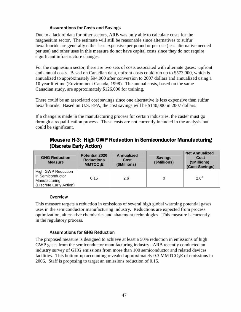
47
Assumptions for Costs and Savings
Due to a lack of data for other sectors, ARB was only able to calculate costs for the magnesium sector. The estimate will still be reasonable since alternatives to sulfur hexafluoride are generally either less expensive per pound or per use (less alternative needed per use) and other uses in this measure do not have capital costs since they do not require significant infrastructure changes. For the magnesium sector, there are two sets of costs associated with alternate gases: upfront and annual costs. Based on Canadian data, upfront costs could run up to $573,000, which is annualized to approximately $94,000 after conversion to 2007 dollars and annualized using a 10 year lifetime (Environment Canada, 1998). The annual costs, based on the same Canadian study, are approximately $126,000 for training. There could be an associated cost savings since one alternative is less expensive than sulfur hexafluoride. Based on U.S. EPA, the cost savings will be $140,000 in 2007 dollars. If a change is made in the manufacturing process for certain industries, the caster must go through a requalification process. These costs are not currently included in the analysis but could be significant.
Measure HMeasure HMeasure HMeasure H----3: High GWP Reductio3: High GWP Reductio3: High GWP Reductio3: High GWP Reduction in Semiconductor Manufacturing n in Semiconductor Manufacturing n in Semiconductor Manufacturing n in Semiconductor Manufacturing (Discrete Early Action)(Discrete Early Action)(Discrete Early Action)(Discrete Early Action)
GHG Reduction Measure
Potential 2020 Reductions MMTCO2E
Annualized Cost
($Millions)
Savings ($Millions)
Net Annualized Cost
($Millions) [Cost-Savings]
High GWP Reduction in Semiconductor Manufacturing (Discrete Early Action)
0.15 2.6 0 2.6∆
Overview
This measure targets a reduction in emissions of several high global warming potential gases uses in the semiconductor manufacturing industry. Reductions are expected from process optimization, alternative chemistries and abatement technologies. This measure is currently in the regulatory process.
Assumptions for GHG Reduction
The proposed measure is designed to achieve at least a 50% reduction in emissions of high GWP gases from the semiconductor manufacturing industry. ARB recently conducted an industry survey of GHG emissions from more than 100 semiconductor and related devices facilities. This bottom-up accounting revealed approximately 0.3 MMTCO2E of emissions in 2006. Staff is proposing to target an emissions reduction of 0.15.

48
Assumptions for Costs and Savings
The cost of the proposed measure is based on the assumption that abatement technologies are used for compliance. The $2.6 million total annualized cost estimate ($3.3 million in 2007 dollars) was derived from a June 2001 U.S. EPA report20. This value included the capital, operating and maintenance costs as a single figure for etch abatement systems. The annualized cost is calculated assuming $23.4 million in capital costs, a 5% discount rate, and a 9 year life for the abatement systems.
Measure HMeasure HMeasure HMeasure H----4: Limit High GWP Use in Consumer Products (Discrete 4: Limit High GWP Use in Consumer Products (Discrete 4: Limit High GWP Use in Consumer Products (Discrete 4: Limit High GWP Use in Consumer Products (Discrete Early Action)Early Action)Early Action)Early Action)
GHG Reduction Measure
Potential 2020 Reductions MMTCO2E
Annualized Cost
($Millions)
Savings ($Millions)
Net Annualized Cost
($Millions) [Cost-Savings]
Limit High GWP Use in Consumer Products (Discrete Early Action)
0.25 0.06 0.23 <0.1
Overview
The objective of this measure is to reduce the use of high GWP compounds in consumer products when alternatives are available. To achieve these reductions, consumer product formulations would need to be changed to reduce or eliminate the use of high GWP compounds.
Assumptions for GHG Reduction
The potential reductions for this measure for 2020 were estimated based on the perceived opportunities for reductions of GHG emissions from specific categories of Consumer Products. Emissions of GHG from the specific Consumer Products were determined from formal surveys of manufacturer’s sales and formulation data that were conducted for the 2001, 2003 and 2006 sales years. Further, in June 2008, the Board approved a measure to reduce the GHG emissions from Pressurized Gas Dusters. This measure achieved approximately 0.20 MMTCO2E in 2020. It is anticipated that the remainder of the emission reduction goal could be achieved by adopting GHG standards for other categories of Consumer Products in future rulemakings.
Assumptions for Costs and Savings
The estimated costs attributed to this measure were based on previous consumer products regulations affecting similar categories of products from which emission reductions were anticipated to occur. Specifically, for the Pressurized Gas Dusters, it was estimated that the total costs of the regulation will be approximately $450,000 over ten years or $45,000 a
20 U.S. EPA June 2001, U.S. High Global Warming Potential (High GWP) Emissions 1990-2010: Inventories, Projections, and Opportunities for Reductions, Chapter 6 Cost and Emission Reduction Analysis of PFC, HFC, and SF6 Emissions from the Semiconductor Manufacturing in the United States, pg. 6-6, June 2001.

49
year.21 Additional costs to manufacturers and consumers will likely occur for additional categories that are regulated for GHG emissions.
Measure HMeasure HMeasure HMeasure H----5: High GWP Reduction from Mobile Sources5: High GWP Reduction from Mobile Sources5: High GWP Reduction from Mobile Sources5: High GWP Reduction from Mobile Sources
GHG Reduction Measure
Potential 2020 Reductions MMTCO2E
Annualized Cost
($Millions)
Savings ($Millions)
Net Annualized Cost
($Millions) [Cost-Savings]
Low GWP Refrigerants for New Motor Vehicle Air Conditioning Systems
2.5 0 16
Air Conditioner Refrigerant Leak Test During Vehicle Smog Check
0.5 TBD TBD
Refrigerant Recovery from Decommissioned Refrigerated Shipping Containers
<0.1 TBD TBD
Enforcement of Federal Ban on Refrigerant Release During Servicing or Dismantling of Motor Vehicle Air Conditioning Systems
0.07 – 0.3
20.86∆
TBD TBD
Low GWP Refrigerants for New Motor Vehicle Air Conditioning SystemsLow GWP Refrigerants for New Motor Vehicle Air Conditioning SystemsLow GWP Refrigerants for New Motor Vehicle Air Conditioning SystemsLow GWP Refrigerants for New Motor Vehicle Air Conditioning Systems
Overview
This measure would reduce greenhouse gas emissions by replacing high GWP refrigerants used in California’s MVACs with lower GWP alternatives that also represent better lifecycle climate performance than the current refrigerant. This measure is meant to initially cover those classes of vehicles not included in the AB 1493 (Pavley) regulation: heavy duty and off-road vehicles. The principal benefit of this measure is the reduction of the GWP impact of refrigerant releases through direct and indirect emissions. The measure is fundamentally the same and as proposed in the Early Action Plan.
Assumptions for GHG Reduction
An estimate of the statewide emission inventory is under development for MVAC refrigerants in 2020. Anticipated reductions for 2020 are expected to be 0.7 MMTCO2E for light duty vehicles and 1.8 MMTCO2E for heavy duty vehicles for a total of 2.5 MMTCO2E for a universal phase out of HFC-134a in new and in-use MVACs in California. These projections were based on the current estimated annual leakage rate of R-134a for light duty vehicles and heavy duty trucks. These estimations will be refined as a more robust emission
21See “Initial Statement of Reasons for Proposed Amendments to the California Consumer Products Regulation, May 9, 2008. http://www.arb.ca.gov/regact/2008/cp2008/cp2008.htm.

50
inventory is developed and the likely replacement refrigerants are selected and the split in the market is predicted.
Assumptions for Costs and Savings
Only capital costs were considered in this cost estimate. Additional staff analysis is needed to determine operating costs, cost savings, and economic impacts. The life of potentially new air conditioning systems is expected to be the same as current systems. Capital costs for the introduction of new refrigerants in the California fleet were estimated to be on the order of $150 million by 2020 based on assumptions that changes begin to phase in around 2013. This estimate is based on a European incremental cost per vehicle of $23 to $28 (at an average exchange rate for the following mentioned year) per LDV in 2003 with a six percent annual increase in cost. The estimate includes several vehicle categories: light duty vehicles, heavy duty vehicles, and off-road vehicles. The detailed information for the intermediate years needs to be determined. Actual costs for maintenance will vary depending on the low GWP refrigerant selected. Significant additional analysis is needed to enable and improve cost and performance estimates of the various alternative technologies.
Air Conditioner Refrigerant Lead Test During Vehicle Smog CheckAir Conditioner Refrigerant Lead Test During Vehicle Smog CheckAir Conditioner Refrigerant Lead Test During Vehicle Smog CheckAir Conditioner Refrigerant Lead Test During Vehicle Smog Check
Overview
As originally conceived, the proposed measure may add a refrigerant leak check to the “pass” criteria for the California vehicular inspection and maintenance (I/M) program, Smog Check, for all vehicles that undergo the test. However, additional staff analysis indicates new issues associated with the technical feasibility of the measure that were not originally considered. Thus, further technical assessment is needed. If put in place, all vehicles that pass Smog Check would have motor vehicle air conditioning (MVAC) systems that either leak at or below natural leak rates (to be determined in the measure) or are empty and precluded from further use unless the identified excessive leak is repaired. Inspections of MVACs would be conducted by the Smog Check technician with a portable refrigerant “sniffer” that detects HFC leakage or other means to be determined in the measure. Protocols would be developed for the test, including use of equipment and identification of threshold values to establish repair criteria. Vehicle owners who choose not to repair a leaky MVAC can pass I/M by agreeing to have the remaining refrigerant recovered and their MVAC rendered inoperable.
Assumptions for GHG Reduction
The potential for annual reductions are thus estimated to be from 0.95 MMTCO2E/year as a standalone measure, to 0.48 MMTCO2E/year when considered as an addition to other measures. The estimates are preliminary; realistic values could range from one half to twice the estimates provided. The estimates are based on the following:
• The program would begin in 2011 • All vehicles will use HFC-134a (GWP=1300) in 2011.
Annual sales of R-134a refrigerant in California are assumed to be emitted into the atmosphere annually due to service losses and due to leaking vehicles. These sales are approximately 1.9 MMTCO2E per year.

51
To determine order of magnitude estimates, it assumed that implementation of an MVAC test and repair requirement would reduce leaks and service losses by 50% to an annual leak rate of 0.95 MMTCO2E/ year. (More detailed analyses of the potential reductions are currently underway). Refrigerant entering the state as OEM charge is not included in the emission rate; and refrigerant captured at end of life is not subtracted from the emission rate. (More detailed analyses of the potential reductions are currently underway). Reductions obtained by implementation of this measure might overlap with reductions obtained by other MVAC related measures. To determine order of magnitude estimates, it is assumed that 50% of the MVAC direct emissions will already have been mitigated by other measures, reducing the potential reduction from 0.95 MMTCO2E/year to 0.48 MMTCO2E/year. (More detailed analyses of the potential reductions are currently underway).
Assumptions for Costs and Savings
Each Smog Check station would have to spend about $200~$300 for each hand-held HFC detector. This assumes the hand-held detector approach proves to be the correct approach. Station owners or technicians would have to pay up to $280 per person to train the Smog Check technicians. The initial cost to Smog Check station owners and technicians would be $2M (Instrument costs) + $4M (Training costs) = $6M. These are one time start up costs. Continuing annual costs are not considered because they are assumed to be covered by increases in the consumer price of a smog check. Due to the increased time required by technicians to test MVAC systems, the consumer price of a Smog Check is expected to increase by an amount that has yet to be determined.
Refrigerant Recovery from Decommissioned Refrigerated Shipping ContainersRefrigerant Recovery from Decommissioned Refrigerated Shipping ContainersRefrigerant Recovery from Decommissioned Refrigerated Shipping ContainersRefrigerant Recovery from Decommissioned Refrigerated Shipping Containers
Overview
The purpose of this measure is to mitigate any impacts from releases, either intended or accidental, of refrigerant from decommissioned refrigerated shipping containers. Refrigerated shipping containers may accumulate in major ports and that the refrigeration systems on these containers may leak high-GWP refrigerants such as HFC-134a. In particular, the refrigerant remaining in the decommissioned containers, the leakage from these containers, and refrigerant disposal as the containers approach end-of-life (EOL).
Assumptions for GHG Reduction
It is essential that a needs assessment be performed to get an accurate estimate the annual amount of refrigerants that are available for recovery from decommissioned refrigerated shipping containers. It has been estimated that shipping container activity could double by 2020. If it is assumed that this applies to the decommissioned refrigerated shipping containers as well, then the bank becomes 160,000 to 320,000 MTCO2E based on staff

52
analysis. This estimate represents the upper bound for the possible reduction potential of this mitigation.
Assumptions for Costs and Savings
Very little information on costs and economic impacts is known today about this proposed measure. As part of measure development, an assessment will be performed in order to get a better understanding of the number of refrigerated shipping containers decommissioned each year, the amount of refrigerant remaining, whether there is refrigerant recovery, and the costs associated with the recovery and recycling processes for the remaining refrigerant.
Enforcement of Federal Ban on Refrigerant Release During Servicing or Enforcement of Federal Ban on Refrigerant Release During Servicing or Enforcement of Federal Ban on Refrigerant Release During Servicing or Enforcement of Federal Ban on Refrigerant Release During Servicing or Dismantling of Motor Vehicle Air Conditioning SystemsDismantling of Motor Vehicle Air Conditioning SystemsDismantling of Motor Vehicle Air Conditioning SystemsDismantling of Motor Vehicle Air Conditioning Systems
Overview
An existing federal regulation (40 CFR 82.154) bans the release to the atmosphere of high-GWP refrigerant substance at the end-of-life or during equipment servicing. The current degree of compliance with 40 CFR 82.154 is poorly documented but under review. The goal of this non-regulatory strategy is improved compliance with this regulation prohibiting the venting of certain types of refrigerant, including HFCs, to the atmosphere when MVACs equipment is serviced or dismantled. Venting is avoided by recovering refrigerants with specialized equipment before dismantling or servicing. The recovered refrigerant can be re-used by the owner or transferred to re-processors approved by U.S. EPA for proper disposal. The anticipated approach would emphasize enhanced enforcement of existing federal requirements for recovery via audits of activities and documentation. ARB will be involved in implementing the measure. The appropriate offices of the U.S. EPA, and the local air districts where dismantling activity is taking place will also participate in developing and enforcing the measure. The Department of Motor Vehicles and the Bureau of Automotive Repair will be involved because vehicle scrapping facilities are under their jurisdiction.
Assumptions for GHG Reduction
Reductions from dismantling operations could be expressed as a baseline emission rate times the fraction that is practically recoverable times a goal for fraction of vehicle dismantlers who would be prompted to comply with the federal regulation. None of these values is well known at present. A rough approximation of the potential reductions from dismantling (as presented in the March 2006 Climate Action Team Report and usable until a better alternative is developed) is 0.1 to 0.6 MMTCO2E per year in 2010 (assuming the program will be in effect then) and 0.07 to 0.3 MMTCO2E per year in 2020.
Assumptions for Costs and Savings
Some dismantlers may not have the latest compliant hardware for recovering refrigerants or any equipment at all. Each dismantler who must purchase the equipment would have to spend approximately $3000 to $5000 per unit. The number of units needed would depend on

53
the size of the operation (vehicle throughput). However, this would be an expense that the dismantler has so far avoided only through failure to comply with the existing federal regulation. Thus, this is not a cost burden associated with the proposed strategy. The same statements apply to obtaining certification for technicians who use the recovery equipment, but with minimal anticipated costs. Training for the U.S. EPA’s certification program is offered by various commercial schools. In addition, the Mobile Air Conditioning Society offers free training (a downloadable pamphlet) and a nominal exam fee, so the expense for operator certification should be minimal. There are costs for storage of recovered refrigerant, record-keeping, and the operators’ labor. Again, however, these are expenses already obliged by the federal regulation. Recovered HFC may have some salvage value, but it is slight.
Measure HMeasure HMeasure HMeasure H----6: High GWP Reduction from Stationary Sour6: High GWP Reduction from Stationary Sour6: High GWP Reduction from Stationary Sour6: High GWP Reduction from Stationary Sourcescescesces
GHG Reduction Measure
Potential 2020 Reductions MMTCO2E
Annualized Cost
($Millions)
Savings ($Millions)
Net Annualized Cost
($Millions) [Cost-Savings]
High GWP Recycling and Deposit Program 6.3 1.0 3.6 -2.6∆
Specifications for Commercial and Industrial Refrigeration
4.0 1.24 0.66 1∆
Foam Recovery and Destruction Program
1.0 94.8 0 95
SF6 Leak Reduction and Recycling in Electrical Applications
0.1 0.3 0.4 -0.1
Alternative Suppressants in Fire Protection Systems
0.1 2 0.2 2
Residential Refrigeration Early Retirement Program
0.1 18.9 24.8 -6
Stationary Equipment Refrigerant Management Program Stationary Equipment Refrigerant Management Program Stationary Equipment Refrigerant Management Program Stationary Equipment Refrigerant Management Program
The high-GWP Stationary Equipment Refrigerant Management Program integrates two AB 32 early action measures: High-GWP Recycling and Deposit Program and Specifications for New Commercial and Industrial Refrigeration Systems. These two measures, discussed below, target different areas of the refrigerant value chain for stationary equipment. The Stationary Equipment Refrigerant Management Program approaches the challenge of high-GWP gases management in a more holistic manner integrating all sectors of the value chain.

54
High GWP Recycling and Deposit ProgramHigh GWP Recycling and Deposit ProgramHigh GWP Recycling and Deposit ProgramHigh GWP Recycling and Deposit Program (also known as High GWP Refrigerant (also known as High GWP Refrigerant (also known as High GWP Refrigerant (also known as High GWP Refrigerant Tracking, Reporting, Repair, Deposit, and Recovery)Tracking, Reporting, Repair, Deposit, and Recovery)Tracking, Reporting, Repair, Deposit, and Recovery)Tracking, Reporting, Repair, Deposit, and Recovery)
Overview
The goal of this measure is to reduce leaks of high-GWP refrigerants from stationary refrigeration and air-conditioning systems and improve service practices that maximize reclamation and recycling of refrigerant. The proposed regulatory action would include facility registration; refrigerant leak detection, monitoring, reporting, and recordkeeping; refrigerant distributor, wholesaler, and reclaimer reporting and recordkeeping; refrigerant sales restrictions to only certified technicians; and a refrigerant cylinder deposit program.
Assumptions for GHG Reduction
Business as usual emissions are based on the U.S. EPA Vintaging Model adjusted to the California population, as provided below: Business As Usual Non-Kyoto Kyoto Total Statewide annual emission estimate: 2004 18 5.3 23.3 Statewide annual emission estimate: 2020 15.3 6.6 21.9
The determination of potential GHG emission reductions from business as usual is based on a year-by-year estimate of 1) compliance rates for leak repair and monitoring, and 2) system retrofitting or retirement. Because the refrigeration and air-conditioning industries are already regulated for ozone depleting substances (ODS), the compliance rates are assumed to be higher for these refrigerants. The range of assumptions for the compliance rates with monitoring, leak repair, and system retrofit and replacement are as follows:
• ODS compliance rates begin at 10% and increase from 5% to 15% each year to reach 100% in 2020.
• HFC compliance rates begin at 5% and increase from 5% to 20% each year to reach 100% in 2020.
The replacement rate for ODS systems is high due to the phase-out of use of ODS as a result of the Montreal Protocol. The incremental annual emission reduction would be the estimated BAU emissions multiplied by an incremental compliance rate. Take HFC as an example, the incremental annual emission reduction in 2011 is: 5.3 MMTCO2E x 5% = 0.26 MMTCO2E The incremental annual emission reduction in 2012 is also: 5.3 MMTCO2E x 5% = 0.26 MMTCO2E The total emission reduction for 2012 would be: 0.26 MMTCO2E + 0.26 MMTCO2E = 0.52 MMTCO2E The total emission reduction for 2019 would equal the sum of the incremental annual emission reductions for years 2011 through 2019 = 5.0 MMTCO2E

55
The incremental annual emission reduction in 2020 based on the 2020 BAU emissions is: 6.6 MMTCO2E x 20% = 1.3 MMTCO2E The total emission reduction for 2020 would be: Total 2019 emission reductions of 5.0 MMTCO2E + 1.3 MMTCO2E = 6.3 MMTCO2E
Assumptions for Costs and Savings
Labor and capital costs for monitoring and leak repair and equipment replacement vary for air-conditioning versus refrigeration equipment. The assumptions for cost and cost savings are as follows: Monitoring Costs Cost per Year / Installation General Cost for Monitoring $100 Monitoring Equipment $2,500 Leak Repair Costs Air Conditioning Refrigeration Labor $2,000 $3,000 Parts & Refrigerants $500 $8,000 Replacement $20,000 $500,000 Facility Inventory Air Conditioning Refrigeration Total Number of Systems 86,000 10,000 Assumes 10,000 facilities have both air condition and refrigeration.
Specifications for Commercial and Industrial RefrigerationSpecifications for Commercial and Industrial RefrigerationSpecifications for Commercial and Industrial RefrigerationSpecifications for Commercial and Industrial Refrigeration
Overview
The primary analysis to estimate possible direct emissions reductions was to assume new refrigeration systems installed would use secondary loop refrigeration technology, or technologies that meet the same performance standards as secondary loop technology. Additionally, ARMINES’ also reviewed the energy savings impact of technical options being applied in all installations, e.g., floating head pressure controls and closed display cases.
Assumptions for GHG Reduction
Although commercial and industrial refrigeration inventory research remains in progress, ARB’s refrigeration and air-conditioning (RAC) contractor, ARMINES’, preliminary work (available at: http://www.arb.ca.gov/cc/commref/armines_report_03_625.pdf) suggests that the Total Equivalent Warming Impact (TEWI) of current direct expansion refrigeration systems commonly used is 0.0307 MMTCO2E (approximately two to three times that of a secondary loop system). Based on literature review it is assumed that 250 new commercial refrigeration systems will be installed in California in the 2012 through 2020 time period – approximately 30 per year

56
from 2012 to 2016 and then 25 from 2017 to 2020. The potential emissions from these new stores are estimated as: Direct Expansion (BAU) = 250 stores * 0.0307 = 7.7 MMTCO2E Secondary Loop (Low Range) = 250 stores * 0.0085 = 2.1 MMTCO2E Secondary Loop (High Range) = 250 stores * 0.0126 = 3.1 MMTCO2E The range of potential emissions reductions are determined based on the difference between the total BAU emissions and the secondary loop systems, or similar technology, emissions – or 2.6 to 5.2 MMTCO2E. This range is averaged and rounded resulting in the potential GHG emission reductions of 4.0 MMTCO2E. In addition to installation of secondary loop systems, ARMINES’ also reviewed the energy savings impact of technical options being applied in installations of all commercial refrigeration equipment within a supermarket, e.g., floating head pressure controls and closed display cases. The preliminary estimation of energy savings is 1.6 TWh per year (1,600 GWh per year) or 30% below baseline. This energy savings impact is a component of the 4.0 MMTCO2E discussed above.
Assumptions for Costs and Savings
Based on literature review and discussions with industry stakeholders, the following assumptions were made: The installation costs increase for a secondary loop refrigeration system is 15-20%, or around $100,000, above current DX systems. Increased costs are due to contractor unfamiliarity with new technologies; installation costs are anticipated to reduce to equal installation costs of direct expansion systems after 2016. Operation and maintenance costs for a secondary loop refrigeration system are up to 40% lower than direct expansions systems (annual cost savings of approximately $25,400). Final Cost Estimates are determined as follows: Total Capital Cost per Year = 30 stores * $100,000 = $3,000,000 Total Cost Savings per Year = 30 stores * $25,400 = $762,000 (2012 to 2016) Total Cost Savings per Year = 25 stores * $25,400 = $635,000 (2017 to 2020)
FoamFoamFoamFoam Recovery and Destruction Program Recovery and Destruction Program Recovery and Destruction Program Recovery and Destruction Program
Overview
Plastic insulating foams containing high-GWP blowing agents are used in refrigerators, freezers, building insulation, transport refrigerated units, and miscellaneous sources. When the product or material has reached the end of its useful life, the insulating foam emits high-GWP GHGs after it is shredded or broken during recycling, or disposed of in landfills. The goal of the measure is to reduce these end-of-life emissions to as close to zero as possible, by recovering waste foam prior to disposal and landfilling, and destroying the high GWP GHGs within the foam.

57
Assumptions for GHG Reduction
Staff estimates for GHG reductions apply a best-case scenario that virtually all potential GHG emissions from waste insulating foam can be reduced at end-of-life by recovering waste foam and destroying the GHGs within the foam before it is recycled or landfilled. Based on literature review and discussions with industry stakeholders, the following assumptions were made: Based on the U.S. EPA Vintaging Model estimates, the estimated annual emissions in the U.S. in 2006 from insulating foam were 71.4 MMTCO2E, with 2.6 MMTCO2E from HFC, and the remaining from ODS. Estimated based on the percent of U.S. population residing in California, HFC emissions in California from foams are estimated as 0.3 MMTCO2E in 2006. 2.6 MMTCO2E * 12.2% = 0.3 MMTCO2E The amount of HFC-containing waste foam has increased about 9 percent per year. By 2020, the estimated emissions of HFCs from waste foam in California will be approximately 1 MMTCO2E annually. 0.3 MMTCO2E * (1 + 9%)14 = 1.1 MMTCO2E Staff assumes 100 percent foam recovery and destruction by 2020, or 1 MMTCO2E, rounded from 1.1 MMTCO2E.
Assumptions for Costs and Savings
Cost estimates are preliminary and will be known with greater precision by July 2010 when an ARB research study will be completed for lifecycle analysis cost of recovery and destruction of high-GWP GHGs. Based on literature review the following assumptions and determinations are made in the cost and savings estimate: Foam Processing Facility Investments 36 million pounds of waste appliance and building foam is generated each year; for every 10 pounds of foam there is 1 pound of foam blowing agent used. An appliance foam processing facility can process up to 2.1 million pounds of insulating foam. 17 foam processing facilities are required (36 million pounds foam / 2.1 million pounds per facility). There are currently three facilities in California, so 14 will be required. There are 14 facilities existing in California that could destroy waste foam (3 waste-to-energy plants, and 11 cement kilns); 8 of the existing destruction facilities will accept and destroy foam waste. As a great volume of building foam can go directly to destruction facilities, the need for foam processing facilities is reduced to six.
58
Six new facilities would have to be constructed, at an average cost of 3.6 million dollars each to process waste foam (6 Facilities * $3.6 = $21.6 million). Each facility would last about 20 years, for an annualized facility construction cost of about $1 million per year. Cost of HFC reduction is approximately $100/MTCO2E; annualized to $94/ MTCO2E. Annual cost is $94 million (1 MMTCO2E reduced * $94/ MTCO2E * 1,000 MT/MMT = $94 million). Total cost per year to reduce HFCs from waste insulating foam would be about $95 million ($1 million in facility construction costs + $94 million in foam collection, recovery, and destruction cost, which includes all recovery labor, transportation, and facility operating costs).
SFSFSFSF6666 Leak Reduction and Recycling in Electrical Applications Leak Reduction and Recycling in Electrical Applications Leak Reduction and Recycling in Electrical Applications Leak Reduction and Recycling in Electrical Applications
Overview
This measure will reduce emissions of SF6 within the electric utility sector and at particle accelerators by requiring the use of best achievable control technology for the detection and repair of leaks, and by the recycling of SF6.
Assumptions for GHG Reduction
Staff estimates an annual emission reduction of 0.07 MMTCO2E calculated from a U.S. EPA reduction estimate of 20% for leak detection and repair and 10% for recycling and recovery based on 2020 projected emissions of 0.22 MMTCO2E in California.
Assumptions for Costs and Savings
Annual operating cost is estimated to be $300,000 for leak detection and repair and recycling. It is assumed that all SF6 saved during leak detection and maintenance activities represents a cost savings because the facility SF6 purchase and consumption rate will decrease. The cost savings from reduced consumption and purchase is estimated at $420,000 annually, yielding a net cost savings of $120,000.
Alternative Suppressants in Fire Protection SystemsAlternative Suppressants in Fire Protection SystemsAlternative Suppressants in Fire Protection SystemsAlternative Suppressants in Fire Protection Systems
Overview
This measure will reduce greenhouse gas emissions from fire suppression systems through a variety of potential reduction options including a GWP threshold for fire suppression agents in new systems, leak reductions strategies, and end of life requirements.
Assumptions for GHG Reduction
The goal of the measure is to reduce emissions to less than 0.1 MMTCO2E by 2020 with an effort to ensure that HFC banks grow no more than about 10% between 2012 and 2020. Leak reduction efforts could address installed capacity while alternative suppressants may be used to address emissions from future banks. The impact on emission levels will be greatest once a large percentage of the systems have moved to low GWP agents.

59
Assumptions for Costs and Savings
Costs will differ depending on the implementation of this measure. Costs presented here will be for using low/no GWP alternatives in new total flooding systems instead of HFC-227. Portable systems and leak reduction strategies are expected to be less expensive. Based on U.S. EPA data and assuming replacement lower GWP agents in systems coming on-line between 2010 and 2015, one-time costs vary from $10 million to $12 million for 2012-2015 with annual costs ranging from $200,000 to a savings of $200,000, depending on the substitute gas. For systems coming online between 2015 and 2020 the one-time cost is approximately $3 to 4 million with annual costs ranging from $70,000 to a savings of $70,000. These estimates are in U.S. 2000 dollars. Converting these to 2007 dollars and annualizing the costs using a 15 year lifetime, the annualized capital costs are approximately $1.8 million. Annual operating costs are approximately $0.2 million and savings are approximately $0.2 million.
Residential Refrigeration Early Retirement ProgramResidential Refrigeration Early Retirement ProgramResidential Refrigeration Early Retirement ProgramResidential Refrigeration Early Retirement Program
Overview
This measure involves establishing a voluntary program to upgrade pre-2000, less energy efficient residential refrigeration equipment such as refrigerators and freezers and ensure proper recovery of refrigerants and blowing agents that have a high-GWP. The measure would include developing strategies to support appliance take-back/upgrade and early retirement programs such as the U.S. EPA Responsible Appliance Disposal (RAD) program and EnergyStar program, in addition to programs administered by local utilities to address direct and indirect GHG emission reductions from domestic appliances.
Assumptions for GHG Reduction
Based on literature review and data available through the U.S. EPA RAD Program the following assumptions and determinations are made in the GHG reductions estimate:
• Currently in California up to 1.2 million refrigerators and freezers are disposed of annually.
• Appliances manufactured prior to 1996 used CFC-12 as the refrigerant and CFC-11 as the blowing agent; appliances manufactured from 1996 to 2002 used HFC-134a as the refrigerant and HCFC-141b as the blowing agent; appliances manufactured after 2002 used HFC-134a as the refrigerant and HFC=245fa as the blowing agent
• For domestic appliances the average refrigerant charge is estimated to be 0.5 pound; the average foam blowing agent used is estimated to be 1.0 pound.
• The primary result of this measure is a 25% increase in recycling of appliances to total 1.5 million per year; an increase of 300,000 appliances per year.
• At an appliance end of life 90% of the original refrigerant charge is recovered. • At an appliance end of life 65% of the initial blowing agent is released – 25% during
shredding and an additional 40% after disposal; this GHG emission is mitigated by this measure.
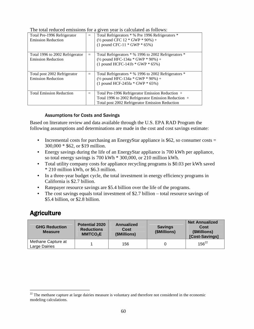
60
The total reduced emissions for a given year is calculated as follows: Total Pre-1996 Refrigerator Emission Reduction
= Total Refrigerators * % Pre 1996 Refrigerators * (½ pound CFC 12 * GWP * 90%) + (1 pound CFC-11 * GWP * 65%)
Total 1996 to 2002 Refrigerator Emission Reduction
= Total Refrigerators * % 1996 to 2002 Refrigerators * (½ pound HFC-134a * GWP * 90%) + (1 pound HCFC-141b * GWP * 65%)
Total post 2002 Refrigerator Emission Reduction
= Total Refrigerators * % 1996 to 2002 Refrigerators * (½ pound HFC-134a * GWP * 90%) + (1 pound HCF-245fa * GWP * 65%)
Total Emission Reduction = Total Pre-1996 Refrigerator Emission Reduction + Total 1996 to 2002 Refrigerator Emission Reduction + Total post 2002 Refrigerator Emission Reduction
Assumptions for Costs and Savings
Based on literature review and data available through the U.S. EPA RAD Program the following assumptions and determinations are made in the cost and cost savings estimate:
• Incremental costs for purchasing an EnergyStar appliance is $62, so consumer costs = 300,000 * $62, or $19 million.
• Energy savings during the life of an EnergyStar appliance is 700 kWh per appliance, so total energy savings is 700 kWh * 300,000, or 210 million kWh.
• Total utility company costs for appliance recycling programs is $0.03 per kWh saved * 210 million kWh, or $6.3 million.
• In a three-year budget cycle, the total investment in energy efficiency programs in California is $2.7 billion.
• Ratepayer resource savings are $5.4 billion over the life of the programs. • The cost savings equals total investment of $2.7 billion – total resource savings of
$5.4 billion, or $2.8 billion.
AgricultureAgricultureAgricultureAgriculture
GHG Reduction Measure
Potential 2020 Reductions MMTCO2E
Annualized Cost
($Millions)
Savings ($Millions)
Net Annualized Cost
($Millions) [Cost-Savings]
Methane Capture at Large Dairies
1 156 0 15622
22 The methane capture at large dairies measure is voluntary and therefore not considered in the economic modeling calculations.

61
Measure: Methane Capture at Large DairiesMeasure: Methane Capture at Large DairiesMeasure: Methane Capture at Large DairiesMeasure: Methane Capture at Large Dairies
Overview
This is a voluntary measure to encourage the installation of methane digesters to capture methane emissions from the decomposition of solid and liquid waste at large dairies. The methane could be used as an alternative to natural gas in combustion, power production, or as a transportation fuel.
Assumptions for GHG Reduction
1,781,799 Head Total California Herd6.55 Million Metric Tons Uncontrolled GHG emissions from California
Herd
1,392,888 Head Total SJVAPCD Herd*78% SJVAPCD percentage of total California Herd
330,028 Affected Head Assumes 73% of dairy cows at dairies with 1,000+ head will already be feeding digesters through voluntary action.
1,223,854 Head Dairy cows, heifers, calves, and bulls at dairies with 1,000+ head not feeding an existing digester
3.676 tonnes CO2e/head Includes CH4 and N2O1.2 Million Metric Tons Uncontrolled emissions from 330,028 head86% Control1.0 Million Metric Tons Reductions from 330,028 head330 Dairies with 1,000 or more dairy cows, heifers,
calves, and bulls not already feeding a digeser
1,628 Total dairies in California (2006 CDFA data)
*: Includes all cows in Kern County
Manure Management Emission Reduction Assumptions (dairies with 1,000 head or more)
Assumptions for Costs and Savings Assumptions for Costs and Savings Assumptions for Costs and Savings Assumptions for Costs and Savings
Staff estimates an operating cost of $33M and an annualized cost for installation of digesters at $123M for this measure based on an average capital cost of $3.9M per digester. No savings is assumed. However, the cost for this voluntary measure is not included in the economic modeling as the reduction is not required as part of the AB 32 GHG emissions reduction program.

62
Cost and Savings Calculation Cost per digester $3.9M # of large dairies (with more than 100 head) 330 Capital cost $1,280M Capital life 15 years 15-year CRF 0.09634 Annualized capital cost 2020 (capital cost x CRF) $123.3M Operating cost 2020 ($100k) $33M Total cost 2020 $156M
ForestsForestsForestsForests
GHG Reduction Measure
Potential 2020 Reductions MMTCO2E
Annualized Cost
($Millions)
Savings ($Millions)
Net Annualized Cost
($Millions) [Cost-Savings]
Sustainable Forest Target
5 50 0 50
Measure: Sustainable Forest TargetMeasure: Sustainable Forest TargetMeasure: Sustainable Forest TargetMeasure: Sustainable Forest Target
Overview
Reductions from this target will be achieved through conservation, forest management, reforestation, afforestation urban forestry and fuels management projects. The forest net flux, that is the balance between uptake and emissions, is currently -5 MMTCO2E.
Assumptions for GHG Reduction
A target reduction of 5 MMTCO2E is required forest sector to maintain the current net flux based on inventory projections.
Assumptions for Costs and Savings
Staff estimates a net cost of $50M to achieve a 5 MMTCO2E reduction based on the current voluntary offset price of approximately $10 per MTCO2E.