Climate change and heat-related mortality in six cities

ORIGINAL PAPER

Climate change and heat-related mortality in six citiesPart 1: model construction and validation

Simon N. Gosling & Glenn R. McGregor & Anna Páldy

Received: 5 October 2006 /Revised: 6 February 2007 /Accepted: 12 February 2007 / Published online: 9 March 2007# ISB 2007

Abstract Heat waves are expected to increase in frequencyand magnitude with climate change. The first part of astudy to produce projections of the effect of future climatechange on heat-related mortality is presented. Separate city-specific empirical statistical models that quantify significantrelationships between summer daily maximum temperature(Tmax) and daily heat-related deaths are constructed fromhistorical data for six cities: Boston, Budapest, Dallas,Lisbon, London, and Sydney. ‘Threshold temperatures’above which heat-related deaths begin to occur are identified.The results demonstrate significantly lower thresholds in‘cooler’ cities exhibiting lower mean summer temperaturesthan in ‘warmer’ cities exhibiting higher mean summertemperatures. Analysis of individual ‘heat waves’ illustratesthat a greater proportion of mortality is due to mortalitydisplacement in cities with less sensitive temperature–mortality relationships than in those with more sensitiverelationships, and that mortality displacement is no longer afeature more than 12 days after the end of the heat wave.Validation techniques through residual and correlation anal-yses of modelled and observed values and comparisons withother studies indicate that the observed temperature–mortalityrelationships are represented well by each of the models. Themodels can therefore be used with confidence to examinefuture heat-related deaths under various climate changescenarios for the respective cities (presented in Part 2).

Keywords Mortality . Climate change . Temperature .

Mortality displacement . Heat waves

Introduction

Both warm and cold extremes of temperature have adverseeffects on health. A non-monotonic ‘V-shaped’ relationshipis often observed between temperature and mortality—annually (Huynen et al. 2001) and for the separate warmand cold seasons (Ballester et al. 1997). Hajat et al. (2006)have shown that, although linear relationships exist be-tween temperature and mortality, during extreme heatevents mortality exceeds that expected from a linearassociation and is better represented non-linearly. Kalksteinand Davis (1989) describe a ‘threshold temperature’ beyondwhich mortality increases above the baseline level. Differ-ent thresholds have been identified for a variety of causesof death (Páldy et al. 2005; Huynen et al. 2001). Thresholdsmay be confounded by other meteorological variables, e.g.Saez et al. (2000) illustrated a 2°C higher threshold (23°C)on very humid days when the relative humidity was above85% in Barcelona, Spain, but there is also evidence thathumidity may have insignificant effects on mortality(Dessai 2002, 2003; Ballester et al. 1997; Braga et al.2001). Thresholds have also been found to vary temporallyfor a single location (Davis et al. 2003; Ballester et al.1997), and according to age, with elderly populations beingmost susceptible to changes in temperature (Conti et al.2005; Donaldson et al. 2003; Huynen et al. 2001).Interestingly, there is evidence that cardiovascular fitnessmay be more important than age in determining individualvulnerability to heat (Havenith 1997). Havenith et al.(1995) examined the response to heat stress across aheterogeneous sample of 56 individuals aged 20–73 years

Int J Biometeorol (2007) 51:525–540DOI 10.1007/s00484-007-0092-9

S. N. Gosling (*) :G. R. McGregorDepartment of Geography, King’s College,London WC2R 2LS, UKe-mail: [email protected]

A. PáldyJozsef Fodor National Institute of Environmental Health,Budapest, Hungary

in a warm humid climate of 80% relative humidity and35°C air temperature. The effect of age was negligiblecompared with effects related to fitness, which wasmeasured by maximum oxygen uptake. Comparativestudies have shown the occurrence of geographical varia-tion in thresholds. Heat-related/cold-related mortalitythresholds occur at higher/lower temperatures in locationswith a relatively warmer/colder climate, and the gradient (orsteepness) of the temperature–mortality relationship forincreasing/decreasing temperature is often found to belower in warmer/colder locations than colder/warmer ones(Donaldson et al. 2003; Pattenden et al. 2003; Keatinge etal. 2000; Eurowinter 1997). For example, Curriero et al.(2002) illustrated across 11 US cities that thresholdtemperatures were higher in warmer southern cities, wherethe temperature–mortality association was less sensitive,than in cooler northern cities. The variation of thresholdsand temperature–mortality gradients has led to inference onhow populations may acclimatise to changing climaticconditions (Donaldson et al. 2003; Curriero et al. 2002;Braga et al. 2001; Saez et al. 2000).

The direct effects of extreme temperature on health arenot always immediate—a lag is often observed between thetemperature event and resultant mortality whereby separateprevious days’ temperatures or lagged moving averages areassociated with the current day’s mortality. Lags of lessthan 3 days are most commonly associated with heat-related mortality (Hajat et al. 2002; Michelozzi et al. 2005;Conti et al. 2005) but different lags may be associated withdisease-specific mortalities (Gemmell et al. 2000; McGregor1999; Páldy et al. 2005; Ballester et al. 1997). Some studiespresent a negative relationship between hot temperaturesand mortality for lags above 3 days, which compensatessome of the deaths caused by heat during the initial days ofthe heat event (Hajat et al. 2002, 2005; Pattenden et al.2003; Braga et al. 2001). This is known as ‘mortality dis-placement’, whereby the heat principally affects individuals

whose health is already compromised and who would havedied shortly anyway, regardless of the weather. Estimates ofmortality displacement vary considerably—Sartor et al.(1995) estimated that 15% of total deaths during theBelgium 1994 heat waves were due to displacement.Gouveia and Fletcher (2000) estimate mortality displace-ment as about 50% during the 1994 heat waves in theCzech Republic. Estimates varied between 1% and 30% inFrance during the summer heat wave of 2003 (Le Tertre etal. 2006) and evidence from the United States estimates thevalue as between 25% and 50% (Kalkstein 1993).

A number of studies point to increases in heat-relatedmortality under climate change scenarios. Donaldson etal. (2001) estimate a 253% increase in annual heat-related mortality by the 2050s for the United Kingdom,and Dessai (2003) estimated the heat-related mortalityrate to increase from between 5.4 and 6.0 (per 100,000)for 1980–1998 to between 5.8 and 15.1 for the 2020s,and 7.3 to 35.6 for the 2050s for Lisbon. The range invalues was due to the combined uncertainties inherent inclimate change projections, potential acclimatisation, andmethodologies.

Assessments of the impacts of climate change on heat-related mortality need to be location specific because it hasbeen shown that the relationship is not evenly distributed inspace (Davis et al. 2004; Kalkstein and Davis 1989).Attention also needs to be paid to the inherent uncertaintiesin impact assessments, especially those arising from climateprojections, so that a range of possible impacts areillustrated. This paper summarises the first part of a studyaimed at producing projections of the effect of futureclimate change on heat-related mortality. The research ispublished in two parts (Fig. 1). In this paper (Part 1)separate empirical–statistical non-linear regression modelsbased on the aggregate dose-response relationship betweendaily maximum temperature (Tmax) and heat-related deaths(the difference between observed and expected deaths) are

Fig. 1 The adopted methodology for this research (adapted from Dessai 2002)

526 Int J Biometeorol (2007) 51:525–540

developed for six cities in order to model the currentrelationship between weather and heat-related mortality. InPart 2, climate change and population change scenarios areapplied to the models developed here to estimate the heat-related mortality burden attributable to climate change foreach city. This includes an exploratory uncertainty analysisto examine the uncertainties in the projections due toclimate modelling, which is considered as a major source ofuncertainty in climate-health modelling (Dessai 2003).Uncertainties concerning acclimatisation and those inherentin the temperature–mortality models are also included.Additional uncertainties such as population ageing and useof air-conditioning/heating units exist, but will not beexamined due to the added complexities in modelling them.

Materials and methods

Selection of cities

The cities selected for this study were Boston, Budapest,Dallas, Lisbon, London and Sydney (Table 1). The aim wasto include cities in different climates such as ContinentalCool Summer, Temperate, Humid Subtropical and Medi-terranean (McKnight and Hess 2000) so that any regionaldifferences in exposure–response could be examined.Another important consideration was that data for at least10 years was available to provide a reliable representationof the cities’ climates, and that it was available atreasonable cost.

Mortality data

Daily total deaths from all causes were obtained for eachcity to include both heat stroke and any possible comorbidfactors (Davis et al. 2003; Kilbourne 1997; Kunst et al.1993). The maximum available data record for each citywas examined because this gives a more reliable represen-tation of climate and any associations with mortality, andgives more precise regression coefficients than if shorterperiods were used (Davis et al. 2003; Horst 1966).Therefore this study assumes that exposure–responserelationships remain constant over time. Davis et al.(2004) state that this stationary nature is often assumed inassessments such as this, but it is noted that some evidencepoints to the possibility of non-stationarity in several UScities (Davis et al. 2003).

Mortality data was missing for Dallas 1990, which wasexcluded from the analysis. Any other missing data wasreplaced by linear interpolation. An anomaly resulting from137 extra deaths caused by an airliner accident at Dallas Fort-Worth International Airport on 2 August 1985 (Wikipedia2006) was excluded from the analysis. As the focus of theresearch is heat-related mortality, only the summer months[June, July, August (December, January, February forSydney); hereafter referred to as ‘summer’] were used foranalysis. For inter-city analysis and estimation of futuremortality burdens under climate- and population-changescenarios, mid-year population estimates were obtained orcalculated by linear interpolation between census years asdenominators for the computation of crude mortality rates

Table 1 Sources of data used for each city

City Köppen classification(McKnight andHess 2000)

Meteorologicalstation used

Meteorologicaldata source

Mortality andpopulation datasource

Population dataavailable

Periodof study

Boston (US) Cooler Humid(Continental CoolSummer)

Boston-LoganInternational Airport

US National ClimaticData Centre

US National Centrefor Health Statistics

Census Years1970, 1980,1990, 2000

1975–1998

Budapest(Hungary)

Warmer Humid(Temperate)

Kitaibel Pál Street Hungary NationalMeteorologicalService

Hungary NationalStatistical Office

Annual 1970–2000

Dallas (US) Warmer Humid(Humid Subtropical)

Dallas Fort-WorthInternational Airport

US NationalClimatic Data Centre

US National Centrefor Health Statistics

Census Years1970, 1980,1990, 2000

1975–1998

Lisbon (Portugal) Warmer Humid(Mediterranean)

LisboaGeofísico

PortugueseMeteorologyInstitute

Portuguese NationalInstitute of Statistics

Census Years1981, 1991

1980–1998

Greater London(UK)

Warmer Humid(Temperate)

HeathrowAirport

British AtmosphericData Centre

Office of NationalStatistics

Annual 1976–2003

Sydney (Australia) Warmer Humid(Humid Subtropical)

Observatory Hill Australian Bureauof Meteorology

Australian Bureauof Statistics

Annual 1988–2003

Int J Biometeorol (2007) 51:525–540 527

(per 100,000); unless otherwise stated, all results arepresented in these units.

Strong seasonal cycles in mortality rates could bias ananalysis of heat-related mortality. A common method toremove the inherent seasonality is to convert daily mortalitycounts into daily mortality anomalies or excess mortality bysubtracting from daily mortality counts a stable mortalitybaseline for each day (i.e. an ‘observed−expected’ method;Guest et al. 1999; Dessai 2002). Excess mortality wascalculated using a 31-day moving average (Rooney et al.1998; Dessai 2002), thus standardising the dependentvariable used in the analysis (excess mortality) by removingany long-term trends in death rates (Davis et al. 2003).Excess mortality approximates heat-related deaths fortemperatures above, or equal to, the threshold temperaturesidentified below (Davis et al. 2003; Dessai 2002; Páldy etal. 2005). Although the calculation of excess mortalityfacilitates the comparison of mortality between cities (Daviset al. 2004), strictly speaking the results of this study shouldbe considered as city-specific because the data was not age-standardised to account for differences in demographicsbetween cities. The data required for this was not availableat an affordable cost. Nevertheless, non-adjusted rates havepreviously been used in climate change–health impactassessments (Dessai 2002, 2003).

Meteorological data

Temperature has been shown to be the dominant climatepredictor of mortality (WISE 1999) so daily Tmax wasobtained for the weather stations in Table 1. Also, afterconsideration of the relatively lower reliability of projec-tions of other meteorological variables, such as humidity,from climate models (Covey et al. 2001; Sun et al. 2003)—with which the relationships would ultimately be used—itwas deemed appropriate to use only Tmax. Missing data wasreplaced by linear interpolation. Data for Dallas and Bostonwere converted from degrees Fahrenheit to degrees Celsius.It is acknowledged that outdoor temperature measurementsare not a direct representation of the climate conditions

within buildings, where the majority of deaths occur(Kilbourne 1997) but widespread data on this spatial scaleis non-existent. Table 2 presents the descriptive statistics foreach city’s temperature distribution.

Model construction and validation

Model construction and identification of threshold temper-atures followed the methodology of Dessai (2002), towhich the reader is referred for a detailed description. Theaggregate dose–response relationship between temperatureand mortality was examined by grouping excess mortalityinto 2°C Tmax class intervals and calculating the number ofexcess deaths per day for each interval; 2°C class intervalswere used (after Guest et al. 1999) instead of 1°C intervals(Dessai 2002) because this smoothes the high variability indaily mortality sometimes evident at higher temperatures.The observed threshold temperatures are illustrated inTable 2. It is acknowledged that using 2°C class intervalsreduced the resolution at which thresholds were identifiedbut this was not a major concern because the purpose wasto allow a comparison of thresholds across cities in arelative sense. Non-linear regression analyses were per-formed on the data above the city-specific thresholds. Alltemperature intervals were used in the regression forBudapest because there were only four intervals above thethreshold. Bootstrapped estimates of the 95% confidenceintervals were also calculated. No more than four additiveconstants were included as parameters in any of theregression models because they can be meaningless interms of physical interpretability and increase the risk ofover-fitting (Glick 1978).

Split-sample validation (Snee 1977) was undertaken bysplitting each city’s time-series in half to create respective‘calibration’ and ‘validation’ samples (Camstra andBoomsma 1992; MacCallum et al. 1994). The entireperiods available that were initially used for modelcalibration are hereafter referred to as the ‘whole periods’and the calibration/validation periods are preceded by theyears used for calibration/validation (e.g. Boston 1975–

Table 2 Descriptive statistics for summer maximum temperature (Tmax) and ‘threshold temperatures’ for each city over the periods of record. SDStandard deviation

City Mean(°C)

SD Minimum(°C)

Maximum(°C)

Range(°C)

Skewness Percentile Threshold(°C)

95th 5th

Boston 26.517 4.809 11.1 38.9 27.8 −0.225 33.889 18.333 26Budapest 26.536 4.203 12.7 37.2 24.5 −0.172 33.200 19.465 28Dallas 34.752 3.232 21.1 45.0 23.9 −0.582 39.444 28.889 34Lisbon 26.865 3.885 16.7 41.5 24.8 0.442 33.955 21.100 28London 22.347 3.937 12.4 37.9 25.5 0.395 29.400 16.300 24Sydney 26.130 3.349 16.1 40.9 24.8 0.843 32.275 21.225 26


1986 calibration). The calibration periods used can be seenin Tables 3 and 4. Non-linear regression was performed oneach city’s calibration dataset and the resultant modelsvalidated through correlation and residual analysis—aprocedure also performed on the whole periods. A detaileddescription of this method is provided by Dessai (2002).The calibration and validation samples were then swappedand the procedure repeated.

Lag effects and mortality displacement

To examine the possible influence of lag effects for eachcity, excess deaths per day were calculated as before, butfor different lags up to the 12th previous day’s Tmax

interval. Further lags were not examined because there is arisk of finding non-causal relationships due to chance orseasonal autocorrelation (Ballester et al. 1997). The lagperiod was limited to 12 because this is central in the broadrange of lags examined in the literature, e.g. up to amaximum of 3-day (Hajat et al. 2002), 14-day (Ballester etal. 1997), 20-day (Braga et al. 2001) and 25-day (Pattendenet al. 2003) lags have been examined. A local linearregression smoothing surface with a bandwidth multiplierof 1.00 and normal kernel (Simonoff 1996) was fitted to thelag data to illustrate the basic relationship.

Six ‘heat waves’ were selected, one from each city, toexamine mortality displacement. No formal internationaldefinition of a heat wave exists so these were defined asperiods lasting three or more consecutive days when the

daily Tmax was equal to, or greater than, the 95th percentileof summer Tmax over the whole period of record. Heatwaves lasting more than 2 weeks according to thisdefinition were excluded from the mortality displacementanalysis because it has been suggested that short-termmortality displacement can be obscured by such lengthyheat episodes (Rooney et al. 1998). The 95th percentile waschosen instead of the 99th because this allows the inclusionof warmer days surrounding the main extremes that mightstill be associated with increases in mortality. Defining heatwaves in this manner yielded several heat waves for eachcity although only one was observed for Sydney. For theremaining cities, the heat wave that included the highestdaily maximum temperature for all heat waves identifiedfor that city was selected for the mortality displacementanalysis.

Results

The non-linear regression analysis for each city yielded theassociations presented in Table 3 and Fig. 2. The associa-tions are all statistically significant (P<0.01). Very high R2

are observed due to the possibility of over-fitting and notincluding any other confounders in the model. However,adjusted R2 R2

a

� �were also calculated and remained high,

suggesting over-fitting was not a major problem.The threshold temperature at which heat-related deaths

become apparent tends to be lower in the cities with a lower

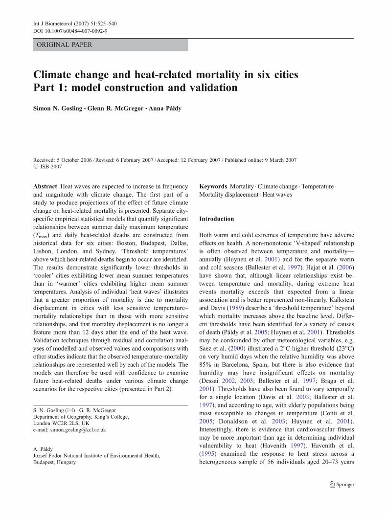
Table 3 Regression forms and coefficients, R2, adjusted R2 R2a

� �F-statistics, and statistical significance of city-specific non-linear regressions

City Regression* Period** a b c d F P R2 R2a

Boston y ¼ aebþ c=xð ÞWhole 1.838 18.062 −689.006 – 121.139 <0.01 0.984 0.9681975–1986 2.904 16.605 −651.199 – 44.337 <0.05 0.972 0.8881987–1998 0.854 9.269 −352.995 – 89.622 <0.05 0.982 0.928

Budapest y ¼ aebþ c=xð Þ þ d Whole 0.822 7.756 −283.200 −0.040 18.289 <0.01 0.887 0.8311970–1985 1.142 8.108 −299.200 −0.085 38.698 <0.01 0.941 0.9121986–2000 0.918 6.917 −252.381 −0.068 13.579 <0.01 0.859 0.789

Dallas y ¼ ebþ c=xð ÞWhole – 16.636 −760.631 – 39.705 <0.01 0.924 0.8731975–1986 – 21.089 −952.167 – 19.000 <0.05 0.878 0.6341987–1998 – 20.798 −952.107 – 13.174 <0.05 0.723 0.446

Lisbon y ¼ aebþ c=xð Þ þ d Whole 3.819 25.424 −1,011.922 0.096 91.691 <0.01 0.988 0.9641980–1988 7.653 34.778 −1,409.933 0.102 28.068 <0.05 0.963 0.8891989–1998 2.754 22.837 −899.971 0.140 600.368 <0.01 0.999 0.995

London y ¼ aebþ c=xð Þ þ d Whole 1.119 7.876 −283.613 −0.020 381.874 <0.01 0.996 0.9881976–1989 0.756 12.891 −429.200 0.000 26.971 <0.05 0.966 0.8301990–2003 1.000 14.248 −513.009 0.071 28.767 <0.01 0.954 0.862

Sydney y ¼ aebþ c=xð ÞWhole 1.000 4.898 −241.200 – 46.743 <0.01 0.917 0.8551988–1995 0.570 6.154 −263.176 – 29.589 <0.01 0.918 0.8361996–2003 0.950 6.275 −288.300 – 11.207 <0.05 0.737 0.474

*Where y is heat-related mortality per day (per 100,000); a, b, c, d are constants; x is the maximum temperature interval**Whole refers to where the entire data period available was used for model calibration, and year–year refers to the calibration periods used forthe split-sample validation


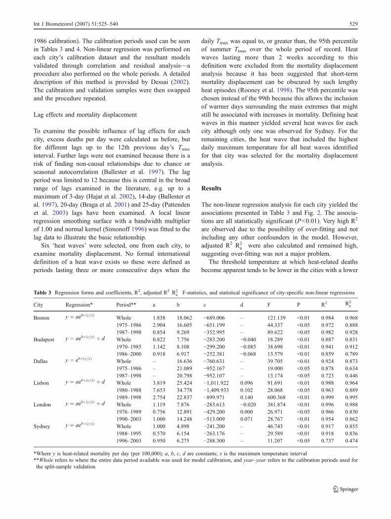
mean summer Tmax than cities with a high mean summerTmax. Plots of threshold temperature against summer meanTmax and variance for each city (Fig. 3) illustrate that meansummer temperature is strongly associated (P<0.01) withthreshold temperature. A weak inverse but statisticallyinsignificant relationship between threshold and summerTmax variance is also evident.

Above the city-specific threshold temperatures, thetemperature–mortality relationships are not homogenousacross cities. Boston is a city with one of the lowest meansummer Tmax values but the highest summer Tmax variance(Table 2) and presents one of the steepest curves. In contrast,Dallas and Sydney, which present the lowest summer Tmax

variances, exhibit the least steep curves. The curve forLisbon is surprising because, opposite to Boston, the city

presents one of the highest mean summer Tmax values andlowest summer Tmax variance. Lisbon’s temperature distri-bution was positively skewed (Table 2), such that the highertemperatures in the distribution were less common, as wasconfirmed by histograms (not shown). When the highertemperatures actually occurred, it is possible heat-relatedmortality was high because the population was lessacclimatised to the occurrence of these infrequent temper-atures. For example, the two highest Tmax intervals occurredonly five times over the whole period in Lisbon, but inBoston they occurred 33 times. The mean number of heat-related deaths per day for Lisbon during these intervals wasapproximately four times greater than for Boston.

For each city, summer Tmax mean and variance wereplotted against the difference between the modelled heat-

Fig. 2 Modelled temperature–mortality associations for each city with extrapolations of 2°C beyond the model calibration temperature with 95%confidence intervals (CI) to give an indication of model uncertainty

Table 4 The heat waves selected to examine mortality displacement in each city, total excess, deficit, net excess, and short-term mortalitydisplacement for the heat wave and following 12 days

City Heat wave date Total excess Deficit Net excess Short-term mortalitydisplacement (%)

Boston 31 July 1975–2 August 1975 329.39 −125.65 203.74 38Budapest 12 July 1991–14 July 1991 50.5 −35.85 14.65 71Dallas 23 July 1977–26 July 1977 62.53 −47.22 15.31 76Lisbon 12 June1981–16 June1981 356.66 −146.68 209.98 41London 3 August 2003–12 August 2003 471.13 −212.67 258.46 45Sydney 5 January 1994–8 January 1994 110.28 −65.28 45.00 59


related deaths for the two highest observed Tmax intervals,which was considered representative of the sensitivity ofthe temperature–mortality relationship (Fig. 3). Neither ofthe relationships were statistically significant.

There is evidence that the magnitude and variability oftemperature will increase with climate change (McGregor etal. 2005; Beniston 2004; Meehl and Tebaldi 2004; Schär etal. 2004), so the curves were extrapolated by 2°C toexamine the relationships beyond the temperature rangesfor which the respective models were calibrated (Fig. 2).The Lisbon model appeared extremely sensitive to anincrease in temperature, whereby a 2°C increase effectivelyincreased the number of heat-related deaths fourfold,relative to heat-related mortality at 40°C. The models forthe other cities were less sensitive, but it would beunreasonable to extrapolate beyond 2°C for use withclimate change scenarios, and caution would have to beexercised when applying the Lisbon model, perhaps notextrapolating beyond 1°C.

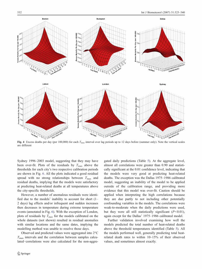
Figure 4 illustrates that the temperature–mortality rela-tionships become steeper with decreasing lag for each city,which justifies using unlagged data for model construction(following Donaldson et al. 2001, 2003). Interestingly, aninverse relationship between temperature and mortality at

lags beyond 3 days for the higher temperatures of thedistribution was apparent, most evidently for Dallas. This ismost likely mortality displacement. One ‘heat wave’ wasselected for each city to further examine this phenomenon.The heat waves are presented in Table 4 and wereconfirmed in the literature for Boston (CLIMB 2004),Lisbon (Dessai 2002), and London (Johnson et al. 2005).Time-series plots indicate mortality deficits (displacement)in the days after the heat waves (Fig. 5). Twelve days afterthe heatwave, daily excess mortality generally stabilizesaround the baseline. Therefore, for each heatwave and thefollowing 12 days, the total number of excess deaths,deficit deaths, the net effect, and short-term mortalitydisplacement contribution (deficit over excess) were calcu-lated, following Le Tertre et al. (2006). The results arepresented in Table 4. With the exception of Budapest, short-term mortality displacement was highest for Dallas andSydney and lowest for Boston and Lisbon—the cities withsome of the weakest and strongest temperature mortalityrelationships, respectively (Fig. 2).

Regarding validation, all the regression models werestatistically significant at the 0.05 or 0.01 level (Table 3).R2 values remained elevated but R2

a values were approxi-mately 30% less than R2 for the two Dallas models and the

Fig. 3 Associations betweensummer mean and standarddeviation (SD) of Tmax andthreshold temperature, and thedifference in modelled excessdeaths for the two highest Tmax

intervals for each city (anestimate of the sensitivity ofthe temperature–mortalityrelationship)


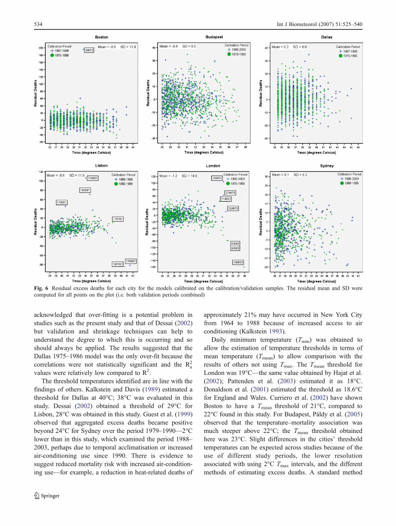
Sydney 1996–2003 model, suggesting that they may havebeen over-fit. Plots of the residuals by Tmax above thethresholds for each city’s two respective calibration periodsare shown in Fig. 6. All the plots indicated a good residualspread with no strong relationships between Tmax andresidual deaths, implying that the models were satisfactoryat predicting heat-related deaths at all temperatures abovethe city-specific thresholds.

However, a number of anomalous residuals were identi-fied due to the models’ inability to account for short (1–2 days) lag effects and/or infrequent and sudden increasesthen decreases in temperature during extreme temperatureevents (annotated in Fig. 6). With the exception of London,plots of residuals by Tmax for the models calibrated on thewhole datasets (not shown) resulted in residual anomalieswith similar locations and the same dates, implying themodelling method was unable to resolve those days.

Observed and predicted values were aggregated into 2°CTmax intervals and the correlation between samples calcu-lated−correlations were also calculated for the non-aggre-

gated daily predictions (Table 5). At the aggregate level,almost all correlations were greater than 0.90 and statisti-cally significant at the 0.01 confidence level, indicating thatthe models were very good at predicting heat-relateddeaths. The exception was the Dallas 1975–1986 calibratedmodel, suggesting an inability of the model to be appliedoutside of the calibration range, and providing moreevidence that this model was over-fit. Caution should beapplied when interpreting the high correlations becausethey are due partly to not including other potentiallyconfounding variables in the models. The correlations wereweak-to-moderate when the daily predictions were used,but they were all still statistically significant (P<0.01),again except for the Dallas’ 1975–1986 calibrated model.

Further validation involved examining how well themodels predicted the total number of heat-related deathsabove the threshold temperatures identified (Table 5). Allthe models performed well, generally predicting total heat-related death rates to within 10–15% of their observedvalues, and sometimes almost exactly.

Fig. 4 Excess deaths per day (per 100,000) for each Tmax interval over lag periods up to 12 days before (summer only). Note the vertical scalesare different


Discussion

Common epidemiological methods for modelling tempera-ture–mortality associations relate the log-expected deathcount to explanatory variables and confounders known tohave some association with mortality, including air-conditioning, air pollution, access to healthcare, and dayof the week for example (Páldy et al. 2005; O’Neill et al.2003; Pattenden et al. 2003; Curriero et al. 2002; Hajat etal. 2002). Such models are useful in that they adequatelyaddress confounding factors but if future climate scenariosare to be applied, reliable projections of confoundingvariables in line with the climate scenarios used (e.g. SRESscenarios; Nakićenović and Swart 2000) are required andmay be unavailable. Obtaining data on confoundingvariables is difficult and/or expensive, especially for severalcities at once. There is also evidence that potentialconfounders have little association with temperature-relatedmortality, e.g. socio-economic status (Gemmell et al. 2000;Guest et al. 1999) and air pollution (Pattenden et al. 2003;Páldy et al. 2005; Hajat et al. 2002). For this reason, severalclimate change–health impact studies have developedsimple temperature–mortality models with temperatureand mortality as the independent and dependent variables,respectively (Davis et al. 2004; Dessai 2002; Guest et al.1999)—a method that was also adopted here.

Application of this method meant the models wereconstructed from the aggregate dose-response relationship

between temperature and mortality, such that they werebased on a small sample of independent–dependentvariables or observations (less than 10) but in some casesused up to four constants to fit the model. It has beensuggested that 10–15 observations should exist for eachconstant or there is a risk of over-fitting the models to thedata (Green 1991; Peduzzi et al. 1996). The implicationsare that over-fitted models may perform extremely well onthe calibration data but not on non-calibration data.However, split-sample validation illustrated that the mod-eling techniques generally performed well outside of thecalibration range—evidence that over-fitting had not oc-curred. One exception was the Dallas 1975–1986 model.

The over-optimism associated with over-fit models canalso be better understood by using shrinkage techniquessuch as the adjusted R2 R2

a

� �; which is dependent on the

number of estimated parameters (p) as well as theproportion of total sum of squares explained (Dunn et al.2003). R2 remains constant or increases as p increases butR2a can decrease and so provides a better estimate of any

over-optimism. For example, note the respective differencesbetween the R2

a and R2 for the Dallas 1975–1986 andSydney 1996–2003 models in Table 3, which suggestssome over-fitting. The R2 values presented by Dessai(2002) are therefore an over-optimistic representation ofmodel quality and hide the possibility that the models wereover-fit. Bootstrapping (Efron and Tibshirani 2003) isanother shrinkage technique and was applied here. It is

Fig. 5 Daily excess mortality (primary y-axis) and Tmax (secondary y-axis) for the heat waves selected for each city. The dates of the last day ofeach heat wave and the 12th day after this are annotated


acknowledged that over-fitting is a potential problem instudies such as the present study and that of Dessai (2002)but validation and shrinkage techniques can help tounderstand the degree to which this is occurring and soshould always be applied. The results suggested that theDallas 1975–1986 model was the only over-fit because thecorrelations were not statistically significant and the R2

a

values were relatively low compared to R2.The threshold temperatures identified are in line with the

findings of others. Kalkstein and Davis (1989) estimated athreshold for Dallas at 40°C; 38°C was evaluated in thisstudy. Dessai (2002) obtained a threshold of 29°C forLisbon, 28°C was obtained in this study. Guest et al. (1999)observed that aggregated excess deaths became positivebeyond 24°C for Sydney over the period 1979–1990—2°Clower than in this study, which examined the period 1988–2003, perhaps due to temporal acclimatisation or increasedair-conditioning use since 1990. There is evidence tosuggest reduced mortality risk with increased air-condition-ing use—for example, a reduction in heat-related deaths of

approximately 21% may have occurred in New York Cityfrom 1964 to 1988 because of increased access to airconditioning (Kalkstein 1993).

Daily minimum temperature (Tmin) was obtained toallow the estimation of temperature thresholds in terms ofmean temperature (Tmean) to allow comparison with theresults of others not using Tmax. The Tmean threshold forLondon was 19°C—the same value obtained by Hajat et al.(2002); Pattenden et al. (2003) estimated it as 18°C.Donaldson et al. (2001) estimated the threshold as 18.6°Cfor England and Wales. Curriero et al. (2002) have shownBoston to have a Tmean threshold of 21°C, compared to22°C found in this study. For Budapest, Páldy et al. (2005)observed that the temperature–mortality association wasmuch steeper above 22°C; the Tmean threshold obtainedhere was 23°C. Slight differences in the cities’ thresholdtemperatures can be expected across studies because of theuse of different study periods, the lower resolutionassociated with using 2°C Tmax intervals, and the differentmethods of estimating excess deaths. A standard method

Fig. 6 Residual excess deaths for each city for the models calibrated on the calibration/validation samples. The residual mean and SD werecomputed for all points on the plot (i.e. both validation periods combined)


for calculating these parameters would therefore aid inter-study comparisons in the future. Nevertheless this study isadvantageous because it applied a common methodologyacross all six cities and the results largely corroborate thefindings of others that have used various methodologies.

Figure 3 illustrates that threshold temperatures werehigher in cities with a higher mean summer Tmax. It couldalso be inferred that temperature–mortality relationshipswere steeper in cooler cities but this would be based on avery weak relationship. Nevertheless, there is evidence tosupport these findings. Curriero et al. (2002) compared 11US cities, illustrating that threshold temperatures werehigher in warmer southern cities where the temperature–

mortality association was less sensitive than in coolernorthern cities. Donaldson et al. (2003) observed steepertemperature–mortality relationships coupled with lowerthresholds in cooler climates by examining southern Fin-land, south-east England, and North Carolina (USA).

The role of temperature variability was shown to beinsignificant. This is surprising given that Braga et al.(2001) observed that, at 30°C, the highest risk of mortalityacross 12 US cities was in cities with a higher variance ofsummertime temperature, and Chesnut et al. (1998)illustrated that summer temperature variability explainedmost of the variation in summer heat-related mortalityacross 44 US cities. These results suggest that acclimatisa-

Table 5 Pearson correlation coefficients and significance between observed (Obs) and predicted (Mod) mortality for mortality aggregated into2°C Tmax intervals (Agg) and non-aggregated values (Daily), respectively; and observed and predicted heat-related deaths for each city (summeronly; death rates are calculated using the mean population during the respective validation periods) with 95% confidence intervals shown inparenthesis

City Period Datalevel

Correlationcoefficient

P Datasource

Totaldeaths

Death rate (per 100,000)per year

Boston Whole Agg 0.995 0.000 Obs 3,668 4.1Daily 0.310 0.000 Mod 3,343 (2,008, 5,563) 3.7 (2.2, 6.2)

1975–1986 Agg 0.995 0.005 Obs 1,578 3.4Daily 0.280 0.000 Mod 1,650 (789, 3,451) 3.6 (1.7, 7.5)

1987–1998 Agg 0.962 0.009 Obs 1,997 4.5Daily 0.341 0.000 Mod 2,210 (1,970, 2,468) 5.0 (4.4, 5.6)

Budapest Whole Agg 0.989 0.001 Obs 3,874 6.2Daily 0.273 0.000 Mod 3,965 (596, 7,784) 6.4 (1.0, 12.5)

1970–1985 Agg 0.991 0.001 Obs 2,144 7.3Daily 0.297 0.000 Mod 2,351 (881, 3,878) 8.0 (3.0, 13.2)

1986–2000 Agg 0.978 0.004 Obs 1,730 5.3Daily 0.242 0.000 Mod 1,982 (792, 3,879) 6.0 (2.4, 11.8)

Dallas Whole Agg 0.954 0.003 Obs 731 1.3Daily 0.090 0.001 Mod 872 (534, 1,424) 1.5 (0.9, 2.5)

1975–1986 Agg 0.986 0.106 Obs 196 0.6Daily 0.046 0.632 Mod 159 (111, 228) 0.5 (0.4, 0.7)

1987–1998 Agg 0.959 0.002 Obs 312 1.3Daily 0.104 0.005 Mod 246 (131, 461) 1.0 (0.5, 1.9)

Lisbon Whole Agg 0.997 0.000 Obs 1,894 4.8Daily 0.465 0.000 Mod 2,114 (1,211, 3,302) 5.4 (3.1, 8.4)

1980–1988 Agg 0.993 0.000 Obs 962 4.7Daily 0.462 0.000 Mod 1,048 (720, 1,689) 5.1 (3.5, 8.2)

1989–1998 Agg 0.943 0.005 Obs 836 4.5Daily 0.502 0.000 Mod 875 (581, 1,520) 4.7 (3.1, 8.2)

London Whole Agg 0.995 0.000 Obs 4,723 2.4Daily 0.444 0.000 Mod 5,369 (1,257, 13,304) 2.8 (0.6, 6.8)

1976–1989 Agg 0.903 0.014 Obs 2,041 2.1Daily 0.344 0.000 Mod 2,521 (1,212, 5,229) 2.6 (1.2, 5.3)

1990–2003 Agg 0.986 0.000 Obs 2,408 2.5Daily 0.465 0.000 Mod 2,476 (1,005, 4,241) 2.6 (1.1, 4.4)

Sydney Whole Agg 0.948 0.000 Obs 1,089 1.8Daily 0.173 0.000 Mod 1,117 (682, 1,807) 1.8 (1.1, 2.9)

1988–1995 Agg 0.839 0.018 Obs 626 1.9Daily 0.169 0.000 Mod 629 (421,883) 1.9 (1.3, 2.7)

1996–2003 Agg 0.957 0.001 Obs 463 1.6Daily 0.173 0.002 Mod 408 (261, 606) 1.4 (0.9, 2.1)

Table 5 Pearson correlation coefficients and significance betweenobserved (Obs) and predicted (Mod) mortality for mortality aggregat-ed into 2°C Tmax intervals (Agg) and non-aggregated values (Daily),respectively; and observed and predicted heat-related deaths for each

city (summer only; death rates are calculated using the meanpopulation during the respective validation periods) with 95%confidence intervals shown in parenthesis


tion occurs in areas that are consistently hot, although it islikely that a higher summertime Tmax variance puts thepopulation at higher risk of heat-related mortality, perhapsdue to an inability to acclimatise to the fluctuatingtemperature, which manifests itself as a lower thresholdtemperature and a steeper temperature–mortality relation-ship. There is no physiological evidence to support this,although the conjecture is often used to explain therelationship between temperature variability and heat-related mortality (Chesnut et al. 1998; Kalkstein 2000). Itshould also be noted that acclimatisation to fluctuatingtemperatures may be less of an issue where high air-conditioning use is common.

Linear fits were applied in Fig. 3 because previousstudies have observed the relationships to be linear byBraga et al. 2001 and Chesnut et al. 1998. However, theselatter studies included 12 and 44 cities, respectively, in theiranalyses. Stronger relationships may have been observedhere if more cities were included in the analysis. It is alsopossible that the relationships may reflect differences inhousing conditions such as age, structure, air-conditioninguse, or prevalence of diseases associated with heat-relatedmortality that have not been controlled for. The role ofsummer mean- and temperature-variability on heat-relatedmortality receives little attention in the literature and furtherstudies would be beneficial, especially as future increases intemperature variability are projected from climate models(Meehl and Tebaldi 2004; Schär et al. 2004).

The models constructed focus on maximum temperatureand have not included diurnal temperature range orminimum temperature. There is evidence that elevatednight temperatures (minimum temperatures) do not allowthe body to recover from the high temperatures experiencedduring the day, increasing mortality risk (Besancenot 2002;Hajat et al. 2002). Minimum temperatures have increasedmore strongly than maximum temperatures over the last30 years (WHO 2003a); a pattern expected to continue withclimate change (Beniston and Diaz 2004). This suggests themodels may not be capturing the complete relationshipbetween temperature and mortality and this should beconsidered when interpreting the results from Part 2 of thisstudy. However, the importance of diurnal temperaturerange is not definitive—Curriero et al. (2002) demonstratedthat a daily diurnal temperature-range variable was unableto significantly predict mortality across 11 US cities.

The models have been constructed from time serieslasting at least 16 years, over which time improvements inhealthcare and infrastructure have occurred. These factorshave not been accounted for in the study, which means ithas been assumed that exposure–response relationshipshave remained constant over time. Davis et al. (2004) statethat such stationarity is often assumed in assessments suchas this. However Davis et al. (2003) have demonstrated that

the US population has become less sensitive to hot andhumid conditions over the past 35 years, despite increas-ingly ‘stressful’ weather. This has been due to improvedmedical care, increased air-conditioning use and betterpublic-awareness programs concerning heat stress. Factorssuch as these might explain why, with the exception ofSydney, the models calibrated on the data of the secondcalibration period often show a flatter increase in mortalitywith temperature or a higher threshold for the mortalityincrease (Table 3), suggesting that the population is lesssensitive to high temperatures. Considering this point, it ispossible the models constructed are not an exact represen-tation of present-day temperature–mortality associationsbecause the model calibration periods include historicaldata from when the population may have been moresensitive to heat.

Furthermore, some climate change may have alreadyoccurred over the calibration periods, especially when morerecent data was used for model calibration, as in the case ofSydney. Also, increased urbanisation will have increasedthe intensity of the urban heat island, the effect of whichwould be more apparent for city centre meteorologicalstations (e.g. Budapest) than those situated at airports (e.g.London). It was decided not to account for any increasingurbanisation or climate change that may have resulted in aclimatic bias over time because the temperature observa-tions for each city should represent the actual conditionsexperienced by their respective residents (Davis et al.2004). However, because the models were calibrated fromaggregated data, any acclimatisation that may have oc-curred due to these increased temperatures will be masked.An important issue concerning the scale of the temperaturemeasurements is that the models were calibrated frompoint-source measurements but the climate model dataapplied to them in Part 2 is gridded, i.e. it has a differentspatial resolution and is not influenced by urban heatislands. In Part 2, gridded observational data is comparedwith the point-source measurements used for modelcalibration here, and the implications of the comparisonsare discussed.

Mortality displacement is often observed during heatwaves but actual estimates of its contribution are not ascommon in the literature as perhaps they should be. Withthe exception of Budapest, short-term mortality displace-ment was highest in Dallas and Sydney—the cities with theweakest temperature mortality relationships—suggestingthat in these cities any heat effects were predominantlymortality displacement. It is conjectured this may bebecause the remaining ‘healthy’ population is well accli-matised to the heat. Supporting this conjecture is that thelowest short-term mortality displacements were for Bostonand Lisbon, the cities with the strongest temperaturemortality relationships, such that the heat significantly


effects the ‘healthy’ population too because it is lessacclimatised to the heat. However, there is no empiricalevidence to support this and the result for Budapest wouldbe contradictory. An explanation for the high displacementpresented by Budapest may be that the heat wave analysedwas preceded by seven other hot days when the temperaturewas above the 90th percentile of daily Tmax, meaning thedisplacement may be due not only to the 3-day heat waveidentified. Indeed, Hajat et al. 2002 showed that mortalitydisplacement for the London August 1995 heat wave mayhave been influenced by another heat wave 2 weeks earlier.Analysis of further heat waves with cooler preceding daysfor Budapest would help to illustrate whether high mortalitydisplacement is a common feature of heat waves inBudapest or whether it was due only to the antecedenttemperatures.

Analysis of the other heat waves identified for each citywould improve the reliability of the mortality displacementestimates. An extensive analysis of mortality displacementis not the focus of this study, however. Nevertheless,previous studies have estimated mortality displacement forone city based on only one heat wave (Gouveia andFletcher 2000; Le Tertre et al. 2006; Sartor et al. 1995). It isacknowledged that it is hazardous to make generalconclusions relating mortality displacement to the sensitiv-ity of temperature–mortality associations based solely onone heat wave for each city because the heat wave chosenfor analysis may not be typical of all heat wavesexperienced by that population. Also, factors other thantemperature may influence the degree of mortality displace-ment and have not been accounted for in this study. Forexample, Hajat et al. (2005) demonstrated that mortalitydisplacement was lowest in Delhi, higher in São Paulo andhighest in London. London included the oldest and richestpopulation; Delhi was the poorest and included the highestproportion of deaths among children. São Paulo’s demo-graphic and epidemiologic profile was between that ofLondon and Delhi.

The large range in short-term mortality displacementobserved in this study, between 38% for Boston and 76%for Dallas, is not unusual—estimates varied between 1%and 30% for nine French cities during the summer heatwave of 2003 (Le Tertre et al. 2006), and Kalkstein (1993)estimated the value as between 25% and 50% for theUnited States. Around 15% of total deaths during theBelgium 1994 heat waves were estimated to be due tomortality displacement (Sartor et al. 1995), and Gouveiaand Fletcher (2000) estimated mortality displacement toaccount for about 50% of total deaths during the 1994Czech Republic heat waves. Further research is required tounderstand what factors influence the differences in theestimates. To some extent, estimates will vary according tothe mortality baseline used to calculate excess deaths. The

results presented are likely to be overestimates because a31-day moving average of mortality was used to calculatethe excess, meaning it is influenced by extremes within thespan. Because displacement estimates are often based onpast events they are not representative of the contributionthat may occur in a present heat wave. Furthermore,estimates can be expected to change temporally becausemortality displacement theoretically depends on the epide-miologic profile of the population at risk (Hajat et al. 2006).

The models were validated by split-sample validation(Snee 1977). The statistical significance of the calibration/validation sample models, which were calibrated on half theavailable data and validated on the remaining half and viceversa, indicated that the regression techniques were validoutside of the calibration range for each city. The respectivemean and SD of residual deaths were generally within thevalues of −1.6 to 0.6 and 9.8 to 13.2 obtained by Dessai(2002). A more complex distributed lag model (Hajat et al.2005; Schwartz 2000) may have resolved the anomalies inFig. 6, as may have calibrating the models only on extremetemperatures such as those above the 99th centile. Howev-er, the inclusion of moderate temperatures is consideredadvantageous because many possible heat-related deathsmay be ignored if these are not included. For example,Hajat et al. (2006) have shown that the burden of heat-related deaths is larger during high-frequency periods whentemperatures are moderate, than during heat waves. Otherthan the anomalies highlighted, the residuals had a goodspread, indicating the models performed similarly well atall temperatures.

The models were able to estimate the moderate andextreme effects of heat on mortality for the whole period, aswell as the calibration/validation periods, with moderate-to-high accuracy. Accuracy is defined as the correlationbetween modelled and observed values (Stewart 2000).Similar to Dessai (2002), correlations on a daily basis werelower than at the aggregate level, but were still statisticallysignificant to at least the 0.05 level. The models were notintended to address the mechanisms affecting daily heat-related mortality—a limitation of many empirical statisticalmodels such as these (McMichael et al. 2001). Instead, theaim was to produce models that reproduced the effects thatclimate has on heat-related mortality as a whole, for whichaggregation was necessary (e.g. Davis et al. 2003; Guest etal. 1999). The lower correlations on a daily basis are aresult of not accounting for these mechanisms, but theeffects climate has on mortality are evident at an aggregatedlevel, for which the correlations were higher. Although thecorrelations are very high, it is important to understand thatthey are due partly to not including other potentiallyconfounding variables in the models.

It was examined how well the models predicted the totalnumber of heat-related deaths above the identified threshold


temperatures (Table 5). This, and the aggregated correla-tions are perhaps a more useful measure of model reliabilitythan the correlations based on daily predictions becausethey consider the total effect that the climate has on heat-related mortality rather than the effect of temperature onindividual days, for which an ‘episode analysis’ method ofassessment would be more appropriate (Páldy et al. 2005;Rooney et al. 1998). The modelled numbers of heat-relateddeaths were usually within 10–15% of the observed valuesfor the periods modelled, similar to that of Dessai (2002).The modelled summer heat-related death rates per yearwere similar to the observed values, and are supported byprevious studies. Kalkstein and Greene (1997) attributed3.5 and 1.2 summer deaths per year (per 100,000) to heatfor Boston and Dallas, respectively. Dessai (2002) attribut-ed between 4.9 and 6.2 for Lisbon. Keatinge et al. (2000)estimated 40 (95% CI, 13, 68) annual heat-related deaths(per million) per year for London—comparable to the 28(95% CI, 6, 68) estimated here.

Comparisons of modelled estimates with those publishedfor documented heat waves further validate the models.Rooney et al. (1998) attributed 184 deaths to heat during the1995 Greater London heat wave (30 July–3 August),representing a 23% excess. The London model predicted170 (95% CI 76, 352) heat-related deaths for the sameperiod, representing a 21% excess. Dessai (2002) showedthat mortality increased by 29% during the Lisbon 1991heat wave (9–18 July)—the Lisbon regression modelpredicted a 38% (95% CI 22, 66) increase over the sameperiod. For Budapest, Páldy et al. (2005) estimated anexcess mortality of 15% (95% CI 7, 23) for the August 1998heat wave (3–5th August), 12% (95% CI 5, 19) for theAugust 1994 heat wave (30 July–8 August), and 15% (95%CI 7, 22) for the August 2000 heat wave (20–22 August)—the Budapest regression model predicted the increases as14% (95% CI 4, 25), 13% (95% CI 4, 24), and 17% (95% CI5, 30) respectively, over the same periods.

The baseline selected to calculate excess deaths variesconsiderably across studies such that mortality estimates aresensitive to the methods used (WHO 2003b). For example,using the moving average of mortality as the baseline(Dessai 2002; Rooney et al. 1998) can result in under-estimates of excess mortality because extreme events areincluded in the span. Conversely, using mortality from theprevious year for the baseline (e.g. Conti et al. 2005) mayoverestimate excess if the previous year was mild. Suchdifferences make comparisons between studies less reliablethan if a standard methodology was employed. Johnson andGriffiths (2003) compared three methods of calculatingseasonal excess mortality for England and Wales andobserved a difference of over 10,000 excess deaths peryear depending upon which baselines were chosen. Com-parisons are also complicated by the length of period used

for analysis. The results of Rooney et al. (1998) and Páldyet al. (2005) are episode analyses based on individualextreme temperature events, which are often criticised foroverestimating mortality due to short-term mortality dis-placement. Although the comparisons made with otherstudies here indicate the developed models produce similarmortality estimates, it should be noted that the differentmethodologies used in different studies may have influ-enced the results.

The mortality estimates used for comparisons across theother studies cited above were calculated from the modelsthat used the whole periods available for calibration.However, extrapolating a model over the same data-rangethat was used to calibrate it may produce an unfair indicatorof model quality because it has been fine-tuned to thecalibration data. For this reason, less attention should beapplied to the correlations and mortality estimates obtainedfrom the whole models than to the calibration/validationmodels presented in Table 5. However, that the correlationsremained high and the mortality estimates were similar tothe observations for the calibration/validation models didsuggest the methodology could produce models that werevalid outside of their calibration range, implying the wholemodels could be applied under climate change scenarioswith confidence. Extreme temperature events will increasein frequency and magnitude with climate change, so, incommon with Dessai (2002), the whole models will be usedin Part 2 because they include all available extremes in thecalibration, which gives a better representation of howmortality varies under such conditions. This was consideredmore important than the inherent limitations associated withvalidating such a model. Ideally, the models used in Part 2would have been calibrated and validated on separatedatasets but until multiple long-term temperature–mortalitydatasets exist for a single, or several nearby locations, suchcompromises are necessary.

Conclusions

Significant relationships between maximum temperatureand heat-related mortality during the summer months havebeen observed and modelled for six cities. Thresholdtemperatures were significantly associated with meansummer Tmax but the role of summer temperature variabilitywas not clear. Estimates of mortality displacement for eachcity have been provided, which are greater in the cities withthe least sensitive temperature–mortality relationships. Theresearch is advantageous because, unlike other assessmentsof the effects of climate change on heat-related mortality(Donaldson et al. 2001; Guest et al. 1999), the models havebeen validated. Split-sample validation procedures andcomparisons with other published papers indicated that the


models reproduced the effects of temperature on heat-relatedmortality well. Furthermore, this highlights the high degreeof insight into temperature–mortality relationships that canbe gained by adopting the relatively simple methodologyapplied here, which excludes possible confounding factorsand concentrates purely on temperature and mortality. Themodels developed can be used reliably to examine thepotential effects of climate change on summertime heat-related mortality in the six cities studied here.

Acknowledgements This study was supported with funding fromthe UK Natural Environment Research Council (NERC) and a Co-operative Awards in Sciences of the Environment (CASE) award fromthe UK Met Office. Thank you to Laurence Kalkstein (University ofMiami), Scott Greene (University of Oklahoma), and Scott Sheridan(Kent State University) for the US data, Suraje Dessai (TyndallCentre) for the Lisbon data, and to Michael Bath (Australian SevereWeather Association) and Robert Van der Hoek (Australian Bureau ofStatistics) for the Sydney data. Thank you also to Allan Baker (Officefor National Statistics) for the London mortality data, and AndreaFulop (Hungary National Meteorological Service) for the BudapestMeteorological data. Jason Lowe is thanked for his comments on anearlier version of the paper.

References

Ballester F, Corella D, Perez-Hoyos S, Saez M, Hervas A (1997)Mortality as a function of temperature. A study in Valencia,Spain, 1991–1993. Int J Epidemiol 26:551–561

Beniston M (2004) The 2003 heat wave in Europe: a shape of things tocome? An analysis based on Swiss climatological data and modelsimulations. Geophys Res Lett DOI 10.1029/2003GL018857

Beniston M, Diaz HF (2004) The 2003 heat wave as an example ofsummers in a greenhouse climate? Observations and climate modelsimulations for Basel, Switzerland. Glob Planet Change 44:73–81

Besancenot JP (2002) Vagues de chaleur et mortalité dans les grandesagglomérations urbaines. Environ Risques Santé 1:229–240

Braga AL, Zanobetti A, Shwartz J (2001) The time course of weather-related deaths. Epidemiology 12:662–667

Camstra A, Boomsma A (1992) Cross-validation in regression andcovariance structure analysis. Sociol Methods Res 21:89–115

Chesnut LG, Breffle WS, Smith JB, Kalkstein LS (1998) Analysis ofdifferences in hot-weather-related mortality across 44 U.S.metropolitan areas. Environ Sci Policy 1:59–70

CLIMB (2004) Climate’s Long-term Impacts on Metro Boston(CLIMB)—Final Report. Civil and Environmental EngineeringDepartment, Tufts University

Conti S, Meli P, Minelli G, Solimini R, Toccaceli V, Vichi M, BeltranoC, Perini L (2005) Epidemiologic study of mortality during theSummer 2003 heat wave in Italy. Environ Res 98:390–399

Covey C, Joussaume S, Kattsov V, Kitoh A, Ogana W, Pitman AJ,Weaver AJ, Wood RA, Zhao Z-C (2001) Model evaluation. In:Houghton JT, Ding Y, Griggs DJ, Noguer M, van der Linden PJ,Xiaosu D (eds) Climate change 2001: the scientific basis-working group 1. Cambridge University Press, UK, pp 471–524

Curriero FC, Heiner KS, Samet JM, Zeger SL, Strug L, Patz JA(2002) Temperature and mortality in 11 cities of the easternUnited States. Am J Epidemiol 155:80–87

Davis RE, Knappenberger PC, Michaels PJ, Novicoff WM (2003)Changing heat-related morality in the United States. EnvironHealth Perspect 111:1712–1718

Davis RE, Knappenberger PC, Michaels PJ, Novicoff WM (2004)Seasonality of climate–human mortality relationships in US citiesand impacts of climate change. Clim Res 26:61–76

Dessai S (2002) Heat stress and mortality in Lisbon. Part 1. Modelconstruction and validation. Int J Biometeorol 47:6–12

Dessai S (2003) Heat stress and mortality in Lisbon. Part II. Anassessment of the potential impacts of climate change. Int JBiometeorol 48:37–44

Donaldson G, Kovats RS, Keatinge WR, McMichael AJ (2001) Heat-and cold-related mortality and morbidity and climate change. In:Maynard RL (ed) Health effects of climate change in the UK.Department of Health, London, pp 70–80

Donaldson GC, Keatinge WR, Näyhä S (2003) Changes in summertemperature and heat-related mortality since 1971 in North Carolina,South Finland, and Southeast England. Environ Res 91:1–7

Dunn G, Mirandola M, Amaddeo F, Tansella M (2003) Describing,explaining or predicting mental health care costs: a guide toregression models. Br J Psychiatry 183:398–404

Efron B, Tibshirani R (2003) An introduction to the bootstrap.Chapman and Hall, London

Eurowinter (1997) Cold exposure and winter mortality from ischaemicheart disease, cerebrovascular disease, respiratory disease, and allcauses in warm and cold regions of Europe. Lancet 349:1341–1346

Gemmell I, McLoone P, Boddy FA, Dickinson GJ, Watt GCM (2000)Seasonal variation in mortality in Scotland. Int J Epidemiol29:274–279

Glick N (1978) Additive estimators for probabilities of correctclassification. Pattern Recogn 10:211–222

Gouveia N, Fletcher T (2000) Time series analysis of air pollution andmortality: effects by cause, age and socioeconomic status. JEpidemiol Community Health 55:750–755

Green SB (1991) How many subjects does it take to do a regressionanalysis? Multivariate Behav Res 26:499–510

Guest CS, Willson K, Woodward AJ, Hennessy K, Kalkstein LS,Skinner C, McMichael AJ (1999) Climate and mortality inAustralia: retrospective study, 1979–1990, and predicted impactsin five major cities in 2030. Climate Res 13:1–15

Hajat S, Kovats RS, Atkinson RW, Haines A (2002) Impact of hottemperatures on death in London: a time series approach. JEpidemiol Community Health 56:367–372

Hajat S, Armstrong BJ, Gouveia N, Wilkinson P (2005) Mortalitydisplacement of heat-related deaths. A comparison of Delhi, SãoPaulo, and London. Epidemiology 16:613–620

Hajat S, Armstrong BJ, Baccini M, Biggeri A, Bisanti L, Russo A,Paldy A, Menne B, Kosatsky T (2006) Impact of high temper-atures on mortality. Epidemiology 17:632–638

Havenith G (1997) Individual heat stress response. Thesis, Springer,Heidelberg

Havenith G, Luttikholt VGM, Vrijkotte TGM (1995) The relativeinfluence of body characteristics on humid heat stress response.Eur J Appl Physiol 70:270–279

Horst P (1966) Psychological measurement and prediction. Wads-worth, England

Huynen MMTE, Martens P, Schram D, Weijenberg MP, Kunst AE(2001) The impact of heat waves and cold spells on mortality ratesin the Dutch population. Environ Health Perspect 109:463–470

Johnson H, Griffiths C (2003) Estimating excess winter mortality inEngland and Wales. Health Stat Q 20:19–24

Johnson H, Kovats RS, McGregor G, Stedman J, Gibbs M, Walton H(2005) The impact of the 2003 heat wave on daily mortality inEngland and Wales and the use of rapid weekly mortalityestimates. Eurosurveillance 10:7–8


http://dx.doi.org/10.1029/2003GL018857

Kalkstein LS (1993) Health and climate change—direct impacts incities. Lancet 342:1397–1399

Kalkstein LS (2000) Saving lives during extreme weather in summer.BMJ 321:650–651

Kalkstein LS, Davis RE (1989) Weather and human mortality: anevaluation of demographic and interregional responses in theUnited States. Ann Assoc Am Geogr 79:44–64

Kalkstein LS, Greene JS (1997) An evaluation of climate/mortalityrelationships in large U.S. cities and the possible impacts of aclimate change. Environ Health Perspect 105:84–93

Keatinge WR, Donaldson GC, Cordioloi E, Martinelli M, Kunst AE,Mackenbach JP, Nayha S (2000) Heat-related mortality in warmand cold regions of Europe: observational study. BMJ 321:670–673

Kilbourne EM (1997) Heatwaves and hot environments. In: Noji EJ(ed) The public health consequences of disasters. OxfordUniversity Press, Oxford, pp 245–269

Kunst AE, Looman CW, Mackenbach JP (1993) Outdoor airtemperature and mortality in The Netherlands: a time-seriesanalysis. Am J Epidemiol 137:331–341

Le Tertre A, Lefranc A, Eilstein D, Declercq C, Medina S,Blanchard M, Chardon B, Fabre P, Filleul L, Jusot J-F, PascalL, Prouvost H, Cassadou S, Ledrans M (2006) Impact of the2003 heatwave on all-cause mortality in 9 French cities.Epidemiology 17:75–79

MacCallum RC, Roznowski M, Mar CM, Reith JV (1994) Alternativestrategies for cross-validation of covariance structure models.Multivariate Behav Res 29:1–32

McGregor GR (1999) Winter ischaemic heart disease deaths inBirmingham, United Kingdom: a synoptic climatological analy-sis. Clim Res 13:17–31

McGregor GR, Ferro CAT, Stephenson DB (2005) Projected changesin extreme weather and climate events in Europe. In: Kirch W,Menne B, Bertollini R (eds) Extreme weather events and publichealth responses. Springer, Berlin, pp 13–23

McKnight TL, Hess D (2000) Physical geography: a landscapeappreciation. Prentice Hall, New Jersey

McMichael AJ, Haines A, Kovats S (2001) Methods to assess theeffects of climate change on health. In: Maynard RL (ed) Healtheffects of climate change in the UK. Department of Health,London, pp 55–69

Meehl GA, Tebaldi C (2004) More intense, more frequent, and longerlasting heatwaves in the 21st century. Science 305:994–997

Michelozzi P, de’Donato F, Bisanti L, Russo A, Cadum E, DeMariaM, D’Ovidio M, Costa G, Perucci CA (2005) Heat waves inItaly: cause specific mortality and the role of educational leveland socio-economic conditions. In: Kirch W, Menne B, BertolliniR (eds) Extreme weather events and public health responses.Springer, Berlin, pp 121–127

Nakićenović N, Swart R (2000) (eds) Special report on emissionscenarios. Cambridge University Press, Cambridge

O’Neill MS, Zanobetti A, Schwartz J (2003) Modifiers of thetemperature and mortality associations in seven US cities. Am JEpidemiol 157:1074–1082

Páldy A, Bobvos J, Vámos A, Kovats RS, Hajat S (2005) The effectof temperature and heat waves on daily mortality in Budapest,Hungary, 1970–2000. In: Kirch W, Menne B, Bertollini R (eds)Extreme weather events and public health responses. Springer,Berlin, pp 99–107

Pattenden S, Nikiforov B, Armstrong BJ (2003) Mortality andtemperature in Sofia and London. J Epidemiol CommunityHealth 57:628–633

Peduzzi PN, Concato J, Kemper E, Holford TR, Feinstein AR (1996)A simulation study of the number of events per variable inlogistic regression analysis. J Clin Epidemiol 49:1373–1379

Rooney C, McMichael AJ, Kovats RS, Coleman MP (1998) Excessmortality in England and Wales, and in Greater London,during the 1995 heatwave. J Epidemiol Community Health52:482–486

Saez M, Sunyer J, Tobias A, Ballester F, Antó JM (2000) Ischaemicheart disease and weather temperature in Barcelona, Spain. Eur JPublic Health 10:58–63

Sartor F, Snacken R, Demuth C, Walkiers D (1995) Temperature,ambient ozone levels and mortality during summer, 1994, inBelgium. Environ Res 70:105–113

Schär C, Vidale PL, Lüthi D, Frei C, Häberli C, Liniger MA,Appenzeller C (2004) The role of increasing temperaturevariability in European summer heatwaves. Nature 427:332–336

Schwartz J (2000) The distributed lag between air pollution and dailydeaths. Epidemiology 11:320–326

Simonoff JS (1996) Smoothing methods in statistics. Springer, BerlinSnee RD (1977) Validation of regression models: methods and

examples. Technometrics 415–428Stewart TR (2000) Uncertainty, judgment, and error in prediction. In:

Sarewitz D, Pielke RA, Byerly R (eds) Prediction: science, decision-making, and the future of nature. Island Press, Washington, pp 41–57

Sun DZ, Fasullo J, Zhang T, Roubicek A (2003) On the radiative anddynamical feedbacks over the equatorial pacific cold tongue. JClimate 16:2425–2432

WHO Regional Committee for Europe (2003a) Heatwaves: impactsand responses. Briefing note for the fifty-third session of theWHO regional committee for Europe, Vienna, 8–11 September2003. WHO, Geneva

WHO Regional Committee for Europe (2003b) Briefing note for thefifty-third session of the WHO regional committee for Europe,Vienna, 8–11 September 2003. WHO, Geneva

Wikipedia (2006) http://en.wikipedia.org. Accessed on 20th August 2006WISE (1999) Weather impacts on natural, social and economic

systems. Final report of work undertaken for the EuropeanCommission Directorate-General Research under contract ENV4-CT97-0448


http://en.wikipedia.org

Documents

Climate change and heat-related mortality in six cities