1

Climate Change and Agriculture in South Asia:

Alternative Trade Policy Options

David Laborde, Csilla Lakatos, Gerald Nelson,

Richard Robertson and Marcelle Thomas

(IFPRI)

in cooperation with Winston Yu and Hans G.P. Jansen

(World Bank)

Pub

lic D

iscl

osur

e A

utho

rized

Pub

lic D

iscl

osur

e A

utho

rized

Pub

lic D

iscl

osur

e A

utho

rized

Pub

lic D

iscl

osur

e A

utho

rized

Pub

lic D

iscl

osur

e A

utho

rized

Pub

lic D

iscl

osur

e A

utho

rized

Pub

lic D

iscl

osur

e A

utho

rized

Pub

lic D

iscl

osur

e A

utho

rized

2

0 Executive Summary

Climate change typically involves changes in water availability and temperature - and both of

these affect crop yields. Changes in crop yields in turn influence prices –of commodities as well

as production factors. Changes in relative factor prices will stimulate their reallocation in the

economy and result in changes in sectoral specialization. Sectoral incomes will be affected

which, together with changes in sectoral specialization, will result in adjustments in sectoral

demand and supply. These changes however, do not occur in a closed economy but at a global

level with heterogeneous effects across countries and commodities. Comparative advantages

evolve, trade patterns adapt and countries are affected by both the domestic effects of climate

change and by changes in relative prices in world markets (terms of trade effects). Over time,

considering income and current account constraints, production will be reallocated across

sectors and across regions to adapt to the exogenous changes in yields. General equilibrium

effects may mitigate or magnify the initial impacts.

Given the complex relationships described above, adequately modeling of the economy-wide

effects of climate change requires linking of climate models (Global Circulation Models) to

economy-wide models (computable general equilibrium or CGE models). In this paper we

combine climate models with a world-wide CGE model to analyze the economic impacts of

climate change in South Asia. First, we use IFPRI’s IMPACT (International Model for Policy

Analysis of Agricultural Commodities and Trade) framework to assess the effects of climate

change (i.e. changes in water availability and temperature) on crop yields under the assumption

of no changes in economic behavior. Subsequently we feed these exogenous changes in a

global computable general equilibrium model (MIRAGE – Modeling International Relationships

in Applied General Equilibrium) to assess the economic impact of climate change. For the

purposes of this paper MIRAGE was expanded to provide a more accurate description of land

use and long term dynamic issues. MIRAGE is also used to analyze the impact of different

climate change scenarios with different socio-economic baselines including alternative trade

policies.

At the global level, South Asia is an important player in terms of production and consumption

of key cereals and other staple foods such as pulses (an important element of South Asia

traditional diet). South Asia has managed to cope with increasing domestic demand for these

3

commodities by improving yields but the region as a whole is not a significant grain exporter. In

an attempt to maintain food security, most South Asian countries protect their domestic grain

markets from world markets through interventionist policies and do not rely on trade.

Nevertheless there exist differences between individual grain crops and across countries. For

example in the case of rice, increases in yields have allowed most South Asian countries to

improve their degree of self-sufficiency. For wheat on the other hand, while India has managed

to export wheat in some years, the smaller economies of the region (Sri Lanka, Nepal,

Bangladesh) remain dependent on large imports. While the overall situation for cereals remains

satisfactory, limited yield gains for pulses have increased the demand-supply gap over time and

made South Asia increasingly dependent on imports.

Continuing increases in crop yields are required in South Asia in order to ensure that supply

keeps up with demand. In this context the slowdown in yield increases seen in the region over

the past decade or so is worrisome and any further perturbation coming from climate change

can lead to a quick deterioration of the regional staple food balance.

The paper begins by investigating to what extent yield increases have impacted self sufficiency

ratios. The results show that while changes in yields may lead to improvement or

deterioration in the degree of domestic self sufficiency, the link is robust only in the case of

rice and depends on the origin of the change in yields - either of short term nature such as

climatic events or of more long term character such as technological change. Yield changes

can be expected to influence land allocation decisions by farmers making modeling such land

use changes important. Yield reductions can be expected to result in price increases which in

turn will translate into demand reductions and detrimental effects on the nutritional status of

especially the poor. Trade liberalization may help to mitigate such price increases and protect

consumers against nutritional shortfalls.

The paper further investigates the link between changes in domestic production and net exports

of South Asian countries. The findings show that countries use trade to balance disruptions in

domestic production in the case of pulses but hardly in the case of cereals. This is due to the

combination of a lack of large storage capacity for pulse crops and more liberal trade policies

compared to cereal crops. For example in Pakistan and India import tariffs on pulses are 50

percent or less compared to tariff on wheat, rice and maize imports.

4

General circulation models (GCMs) were used to translate different green house gas (GHG)

emission scenarios into varying temperature and precipitation outcomes. While the general

consequences of increasing atmospheric concentrations of GHGs are increasingly well known,

great uncertainty remains about how climate change will play out in specific locations.

Therefore this paper relies on 12 alternative climate change scenarios which together help

define the range of potential outcomes from climate change in South Asia. These 12 scenarios

result from combining alternative GHG paths and different GCM models. Yields changes

resulting from alternative climate change scenarios for selected crops (maize, wheat, rice,

soybeans and groundnuts) as estimated by the DSSAT model are discussed. Decreases in

average global yields across the different scenarios vary from 0.6 percent to 11 percent.

Wheat and maize yields are more affected than yields of rice (rainfed) and soybeans even

though the variance across scenarios is higher for the latter. For all crops average yield

changes weighted by initial production levels are larger than average changes weighted by area

–suggesting that high productivity regions will be relatively more affected by climate change

than less productive regions. This could in turn lead to significant changes in trade patterns to

the extent that high productivity regions are currently the main sources of exports. Yield

decreases are largest for wheat and soybean - 11.5 percent and 8.2 percent respectively

(weighted by area). Further decomposition shows that all four South Asian countries considered

in our analysis are negatively impacted, with Pakistan and India most severely affected (showing

average yield decreases of respectively 9.6 percent and 3.9 percent when weighted by initial

production).

The exogenous yield changes coming out of the climate models were fed into a modified

MIRAGE model. Since policy makers have a certain degree of control over trade measures, eight

alternative trade policy scenarios were analyzed that could be implemented between 2010 and

2024. These different trade policy scenarios involve potential tariff reductions from their

starting levels in 2007 with varying degrees of liberalization and regional integration. In this

manner a total of 124 different combinations of trade policies and climate change scenarios

were simulated.

The results confirm that South Asia will be significantly affected in terms of the impact of

climate change on crop yields. Climate change affects both the overall level of economic activity

and trade flows – resulting in an average 0.5 percent decrease in real income for the region as a

5

whole but with big differences across individual countries. For example whereas Pakistan may

suffer an income decrease of up to 4 percent, India is least affected – changes there vary

between a 0.6 percent income decrease to a 0.5 percent increase depending on the climate

change scenario.

Since the share of agriculture in world GDP is expected to continue to decline, and even more so

in a high-growth economy like India’s, the findings regarding the impact of climate change on

real incomes are perhaps not surprising. On the other hand it is important to keep in mind that

this paper models only part of the possible consequences of climate change, i.e. only changes in

crop yields due to changes in precipitation and temperature are taken into account. We do not

consider the possibility of new pest and diseases arising as a result of changes in climatic

conditions, the shift in cattle productivity due to temperature changes, or more generally any

negative productivity shocks associated with a warmer climate. Last but not least, extreme

events (flooding) or loss of agricultural area due to possible rises in sea levels are not taken into

account.

Uncertainty about the exact intensity of climate change and its exact geographical location,

embodied in the 12 SRES scenarios considered in the analysis, has significant impacts in terms of

variability of the results. Based on the simple average between SRES scenarios, it seems that

except for India all other South Asian countries should favor the status quo or the deepening

of regional integration focused on SAFTA. India may have a preference for more ambitious

trade policies consisting of a trade agreement agenda at the pan Asia level or even at a global

scale. Nonetheless, India would need to obtain access to foreign markets in order to choose this

path and unilateral trade liberalization is not an optimal strategy for managing the impact of

climate change since the exact nature, location and effects of climate change remain highly

uncertain.

The specific case of India warrants closer attention since it has implications for the South Asian

region as a whole. On the one hand, India is a large and fast growing country, and by 2050 can

be expected to have even larger market power. Unilateral trade liberalization by India may

expose the country to negative price shocks and large terms of trade losses. By maintaining

trade restrictions, India could use its market power and the traditional “optimal tariff argument”

to mitigate the impact of increases in world prices on domestic prices and limit the deterioration

of its terms of trade. At the same time, India would benefit from the opening of foreign

6

markets. But the strengths of India go even beyond its international market power. The size of

its domestic market enables India to reallocate production factors across crops while allowing

regions to redefine an optimal production pattern compatible with changing climatic conditions.

In particular, India may rely on vast amounts of land currently used for cotton to produce

additional food crops. For smaller countries, such an internal diversification strategy is much

less feasible. This stresses the importance for the region as a whole of having flexible

commodity as well as factor markets in order to ensure sufficient adaptation capacity and

efficient allocation resources.

Besides its effect on real GDP, it is important to consider the distributional impact of climate

change. Our analysis suggests that climate change has a negative impact on the real wage of

unskilled labor (a proxy for poor people’s income). This is not unexpected since unskilled labor

is directly impacted by the change in agricultural productivity. In the case of Pakistan, the losses

exceed 5.5 percent in real terms. For India, while on average the real wage of unskilled labor

increases by 1.6 percent under a status quo policy, the range of uncertainty is large: between

+8.2 percent and -9.1 percent depending on the climate change scenario. For the poor in India

unilateral trade liberalization may be the best strategy. But India is the exception also in this

respect – for the poor in other countries the status quo is preferred, with the exception of the

worst climate change scenario in which case unilateral trade liberalization is also the preferred

strategy for the poor in other South Asian countries.

Even if trade policies are unable to significantly mitigate the impacts of climate change, trade

liberalization can still play an important role in restoring market equilibrium. For example,

South Asia’s imports of major food crops are simulated to increase by 6 percent on average

across all SRES scenarios. Trade liberalization, especially at the world level, would mitigate the

price increases for these food imports. Uncertainties regarding the exact nature of climate

change again lead to widely diverging predictions: global trade in agriculture may increase or

decrease depending on how traditional exporters (e.g. countries belonging to the Cairns group)

would be affected and how traditional importers would need to find new trade partners or

develop domestic solutions. Indeed, agricultural trade liberalization would also lead to

important market opportunities for South Asia in other developed and developing markets.

When climate change occurs, exports can focus on sub regional markets, thus significantly

mitigating crop price increases driven by reductions in yields.

7

Finally, the analytical framework in this paper based on a large number of simulations has

generated valuable information, not only regarding average outcomes but also regarding the

risk driven by climate change of different trade policy options. Adopting a risk analysis approach

and assuming different levels of risk aversion among regional policy makers could provide

guidance regarding the choice of an “optimal” strategy, taking simultaneous account of levels

and variance of expected outcomes (as in a portfolio approach). The degree of hysteresis and

the sunk cost nature of some investments will be very important aspects in assessing the costs

of ex-post modification of trade policy options once they have been chosen ex-ante.

8

Table of Contents

0 Executive Summary ................................................................................................................. 2

1 Introduction ........................................................................................................................... 14

2 Methodology ......................................................................................................................... 17

2.1 Modeling the effects of Climate Change on Crop Yields ............................................... 18

2.1.1 The IMPACT framework ........................................................................................ 18

2.1.2 DSSAT Yield Projections ......................................................................................... 20

2.2 The MIRAGE model for Climate Change Analysis .......................................................... 23

2.2.1 Generic features of the MIRAGE model ................................................................ 25

2.2.2 Adapting MIRAGE for climate change analysis ...................................................... 27

3 Trade policies and patterns, and production and consumption ........................................... 34

3.1 Overview of current tariff barriers ................................................................................ 34

3.1.1 Tariffs on Agricultural Goods ................................................................................. 34

3.1.2 Tariffs on Food Products........................................................................................ 36

3.2 The evolution of trade flows by region ......................................................................... 42

3.2.1 The evolution of trade flows by sector .................................................................. 47

3.2.2 Regional and sectoral decomposition of SAFTA's trade flows .............................. 53

3.2.3 The composition of SAFTA's intra-regional trade .................................................. 58

3.3 The evolution of production, yields, and consumption of agricultural commodities ... 60

3.3.1 Current situation ................................................................................................... 60

3.3.2 Yield fluctuation and domestic demand coverage ................................................ 67

4 Climate change scenarios ...................................................................................................... 75

4.1 Yield impact of Climate Change ..................................................................................... 77

4.1.1 Impact of climate change on global yields ............................................................ 77

4.1.2 Impact on yields in South Asia ............................................................................... 82

5 Trade Policy Scenarios and Simulations Results .................................................................... 90

9

5.1 Trade policy alternatives as different baselines for climate change scenarios ............. 90

5.1.1 Description of trade policy alternatives ................................................................ 92

5.1.2 Baseline results ...................................................................................................... 94

5.2 Simulation Results ......................................................................................................... 95

5.2.1 Impact of climate change and trade policy on real income .................................. 95

5.2.2 Impact of climate change and trade policies on Agricultural Production ........... 100

5.2.3 Impact of climate change and trade policies on Poor People’s Income ............. 104

5.2.4 Impact of climate change and trade policies on Food consumption and Food

prices 106

5.2.5 Impact of climate change and trade policies on Trade ....................................... 112

5.3 Sensitivity analysis based on alternative economic and population growth .............. 121

5.3.1 Consequences of lower GDP growth ................................................................... 122

5.3.2 Consequences of higher population growth ....................................................... 122

6 Concluding Remarks ............................................................................................................ 124

7 References ........................................................................................................................... 129

8 Appendix .............................................................................................................................. 131

10

List of Figures

Figure 1 Modeling Framework ...................................................................................................... 18

Figure 2 Links leading to the incorporation of climate change in IMPACT ................................... 19

Figure 3 Average Tariffs on Agricultural products in 2007 for South Asian countries (Reference

group weighted) ............................................................................................................................ 36

Figure 4 Average Tariffs on Food products for South Asian countries (Reference group weighted)

....................................................................................................................................................... 37

Figure 5 Average Tariffs on Calories for South Asian countries .................................................... 38

Figure 6 Average Tariffs on Fats for South Asian countries .......................................................... 39

Figure 7 Average Tariffs on Proteins for South Asian countries.................................................... 41

Figure 8 Exports and Imports of Calories by Region (billions) ....................................................... 44

Figure 9 Exports and Imports of Proteins by Region (kilotons) ..................................................... 45

Figure 10 Exports and Imports of Fats by Region (kilotons).......................................................... 46

Figure 11 Exports and Imports by Sectors in 103 US dollars ......................................................... 48

Figure 12 Exports and Imports of Calories by Sector (103 metric tons) ........................................ 49

Figure 13 Exports and Imports of Proteins by Sector (103 metric tons) ........................................ 51

Figure 14 Exports and Imports of Fats by Sector (103 metric tons) .............................................. 52

Figure 15 Composition of Exports and Imports (value) ................................................................. 54

Figure 16 Composition of Exports and Imports of Calories ........................................................... 55

Figure 17 Composition of Exports and Imports of Proteins .......................................................... 56

Figure 18 Composition of Exports and Imports of Fats ................................................................. 57

Figure 19 Production, yields and coverage of consumption: Paddy rice ..................................... 62

Figure 20 Production, yields and coverage of consumption: Maize ............................................. 63

Figure 21 Production, yields and coverage of consumption: Wheat ............................................ 64

Figure 22 Production, yields and coverage of consumption: Pulses ............................................. 65

Figure 23 Correlation between variations in coverage and yield - by country ............................. 69

Figure 24 Correlation between variations in coverage and net exports ....................................... 73

Figure 25 Emissions scenarios: change in temperature ................................................................ 76

Figure 26 Changes in world yields (rainfed) due to climate change for different scenarios and

selected crops. Weighted by initial area and production. ............................................................ 78

Figure 27 Distribution of yield changes under alternative climate change scenarios. Weighted by

area (Rainfed). ............................................................................................................................... 80

11

Figure 28 Share of rainfed agriculture at the world level for selected crops................................ 81

Figure 29 Distribution of change in global yield of rice (weighted by production) for rainfed and

irrigated cultivation. ...................................................................................................................... 82

Figure 30 Changes in crop yields in South Asia (rainfed) due to climate change for different

scenarios and selected crops. Weighted by initial area and production. ..................................... 84

Figure 31 Distribution of yield changes under alternative climate change scenarios. Weighted by

area (Rainfed). ............................................................................................................................... 85

Figure 32 Distribution of yield changes across countries under alternative climate change

scenarios. Weighted by production (rainfed). .............................................................................. 87

Figure 33 Share of rainfed agriculture at the world level for selected crops................................ 88

Figure 34 Distribution of yield of selected crops in Pakistan for rainfed and irrigated production

(weighted by production) .............................................................................................................. 89

Figure 35 Annual changes in world real income by 2050 - by climate change scenario and trade

policy alternative ........................................................................................................................... 96

Figure 36 Changes in real incomes in SAFTA countries compared to other regions and countries

(simple averages across climate change scenarios) ...................................................................... 97

Figure 37 Real Income effects (simple averages and extreme values) of climate change in SAFTA

countries – by trade policy alternative .......................................................................................... 98

Figure 38 Average changes in food prices (% changes in 2050 relative to the baseline in each

trade policy alternative) .............................................................................................................. 107

Figure 39 Changes in domestic prices for local varieties of key commodities – averages across

climate change scenarios and trade policy alternatives (% changes relative to the Status quo

trade policy baseline in 2050) ..................................................................................................... 109

Figure 40 Changes in average per capita consumption (% changes relative to the baseline in

2050, simple average across climate change scenarios) for the BASE (status quo) and MULTI

(multilateral trade liberalization) trade policy alternatives ........................................................ 110

Figure 41 Changes in world trade of staple crops (%changes in volume relative to baselines of

trade policy alternatives in 2050) ................................................................................................ 113

Figure 42 Food imports in South Asia (% changes in volumes relative to the baseline for each

trade policy option by 2050) ....................................................................................................... 115

Figure 43 Sectoral composition of import changes for South Asia by trade policy alternative

(simple averages across climate change scenarios – constant 2004 US$ 109)............................ 116

12

List of Tables

Table 1 List of GCM used in our analysis as inputs for climate change effects on temperature and

precipitations ................................................................................................................................. 17

Table 2 Sectoral decomposition of the MIRAGE model ................................................................ 25

Table 3 Regional decomposition of the MIRAGE model ............................................................... 25

Table 4 Bilateral Exports of Calories (106 metric tons) ................................................................. 58

Table 5 Bilateral Exports of Proteins (106 metric tons) ................................................................ 59

Table 6 Bilateral Exports of Fats (106 metric tons) ....................................................................... 59

Table 7 Alternative GCM model results in terms of changes in temperature and precipitation .. 77

Table 8 Summary of trade policy alternatives ............................................................................... 94

Table 9 Baseline trade policy alternative: evolution of selected indicators ................................ 95

Table 10 Summary table of best options for trade policies. Real Income criteria ...................... 100

Table 11 Impact of climate change on agro-food and stale production (% changes in 2050

relative to the baseline in each trade policy alternative) ........................................................... 102

Table 12 Five most negatively affected agricultural commodities by country (% changes in 2050

relative to the baseline in each trade policy alternative) ........................................................... 104

Table 13 Changes in real Unskilled labor Wages (% changes in 2050 relative to the baseline in

each trade policy alternative) ...................................................................................................... 106

Table 14 Standard deviation in the % change of per capita food consumption across climate

change scenarios in 2050 ............................................................................................................ 111

Table 15 Changes in imports of staple and processed foods by country (% change in volumes

relative to the each trade policy option’s baseline by 2050) ...................................................... 118

Table 16 Changes in bilateral agricultural trade flows (% changes in volumes by 2050 compared

to the baseline of each trade policy option) ............................................................................... 119

Table 17 Changes in bilateral agricultural trade flows (in constant 109 2004 dollars by 2050

compared to the baseline of each trade policy option) .............................................................. 120

Table 18 Sensitivity analysis based on alternative assumptions regarding economic and

population growth: selected indicators. Simple averages across climate change scenarios for two

trade policy alternatives. Numbers represent percentage devations from each baseline. ........ 121

Table 19 Detailed real Income effects by country and scenarios. 109 constant USD (2004) ...... 131

13

List of Acronyms

AEZ Agro-Ecological Zone

ASEAN Association of Southeast Asian Nations

ANZCERTA Australia New Zealand Closer Economic Relations Trade Agreement

AVE Ad Valorem Equivalent

CGE Computable General Equilibrium Model

DSSAT Decision Support System for Agrotechnology Transfer

FDI Foreign Direct Investment

FPU Food Production Unit

FTA Free Trade Area

GCM General Circulation Models

GHG Greenhouse Gas

IMPACT International Model for Policy Analysis of Agricultural Commodities and Trade

IPCC Intergovernmental Panel on Climate Change

MIRAGE Modeling Interregional Relations in Applied General Equilibrium

NAFTA North American Free Trade Association

SAARC South Asian Association for Regional Cooperation

SAFTA South Asian Free Trade Area

SRES Special Report on Emissions Scenarios of the Intergovernmental Panel on Climate

Change

TFP Total Factor Productivity

14

1 Introduction

There is increasing evidence suggesting that climate change will negatively impact agricultural

production in South Asia. Decreased domestic production may make South Asian countries

more dependent on imports. Given that (i) world markets for some of the major agricultural

commodities consumed in South Asia are relatively thin (especially rice but also wheat and

pulses) and (ii) the size of domestic markets in South Asia is large and growing, increased import

demands of South Asian countries may result in substantial price increases in world markets and

bring renewed concerns regarding food security and welfare throughout the world.

The extent to which South Asia would need to increase its imports as a result of climate change

would presumably depend on the degree to which the latter would affect domestic output. The

capability of South Asia to import more, and the costs associated with these higher imports,

would in turn depend on the degree to which climate change might have a positive impact on

production elsewhere in the world and lead to higher exportable surpluses. Thus, modeling the

effect of climate change on agricultural production, both regionally in South Asia and worldwide,

is required to be able to assess its impact on global trade in agricultural commodities; and to

analyze the effect on world market prices. At the same time, the capacity of South Asia to tackle

the new situation will depend largely about how growth will increase income and help to

diversify economic activities. Indeed, at the macro level, if agriculture plays an important role in

total GDP for some countries, they will be particularly exposed in the case of negative

productivity shocks in this sector.

The effects of climate change on agriculture may well differ substantially for individual South

Asian countries and indeed for regions within a given country which can be approximated by

food production units (see next Chapter). Besides trade between South Asia as a region and the

rest of the world, intraregional trade between South Asian countries may be able to dampen the

effects of climate change on domestic supplies and prices at the level of the individual countries.

This calls for an analysis of climate change effects on trade flows under alternative trade policy

regimes both for agriculture and non agricultural sectors.

Substantial work has been carried out regarding the welfare benefits of worldwide trade

liberalization (e.g. World Bank DEC, IFPRI etc) using different global trade models. Recently

IFPRI completed a paper for the World Bank regarding the potential benefits of intra-regional

15

trade liberalization in South Asia (Bouet and Corong, 2009) and its effects on prices of

agricultural commodities within the region. The main result was that the effect on domestic

food prices in South Asia of the implementation of trade policies as stipulated in the South Asian

Free Trade Area (SAFTA) agreement would be quite limited.

However, no analytical work has been done so far that reconciles the effects of climate change

on agricultural production with its potential impact on trade flows of agricultural commodities

and corresponding prices. This is important because if climate change is going to substantially

increase South Asia’s import demand and exportable surpluses elsewhere in the world do not

match this increased demand, there is likely to be upward pressure on prices.

The specific objectives of the paper include the following:

Analyze the extent to which agricultural production in South Asia and elsewhere

in the world may be affected by different scenarios regarding climate change.

Analyze the extent to which changes in domestic production in South Asia

resulting from climate change would lead to increased demand for imports by

South Asian countries.

Analyze the effects of increased import demand in South Asia and changing

exportable surpluses elsewhere on world market prices of major agricultural

commodities consumed in South Asia.

To the extent that South Asian governments allow transmission of changes in

world market prices to domestic prices, analyze the potential welfare effects of

changes in the latter.

Analyze if, and to what extent, worldwide trade liberalization and

implementation of SAFTA would dampen the effects of climate change on

domestic agricultural prices in South Asia.

To answer these questions, Chapter II of the paper describes the methodology used - with

particular attention to how different models and modeling techniques are linked to produce an

as accurate as possible assessment based on state-of-the-art knowledge. Chapter III provides an

up-to-date analysis of trade flows, trade policies and production patterns for key food products

in South Asia to explain the context in which climate change is taking place. It also shows the

role of agricultural trade for the region for coping with growing demand, climatic shocks and

16

food security targets. Chapter III also justifies the regional and sectoral disaggregations used in

the paper. Chapter IV describes the climate change scenarios and illustrates their consequences

for crop yields at a global level and for South Asia - and in particular shows the vulnerability of

the region to these changes. Baseline design, simulations and results are discussed in Chapter V.

The final Chapter provides a short summary, discusses the limitations of the analysis and derives

suggestions and guidelines for future research.

17

2 Methodology

Modeling the economic impact of climate change on the agricultural sectors of South Asian

countries by 2050 is a challenging task and requires combining different models. The modeling

framework employed in this paper is depicted in Figure 1. Taking results from different climate

models (Global Circulation Models (GCM) listed in Table 1) regarding the probable evolution of

temperature and rainfall, a number of IFPRI tools that are part of the IMPACT (International

Model for Policy Analysis of Agricultural Commodities and Trade) framework are used to assess

the effects of changes in water availability and temperature on crop yields - while assuming

economic behavior as constant. These exogenous changes are subsequently plugged into the

MIRAGE (Modeling International Relationships in Applied General Equilibrium) global

computable general equilibrium model (CGE) to assess the overall economic consequences of

these evolutions. The CGE model is also used to analyze the different climate change scenarios

with different socio-economic baselines - including alternative trade policies.

Table 1 List of GCM used as inputs for determining climate change effects in terms of changes in temperature and precipitation

Label Description CNR(M) Centre National de Recherches Météorologiques (Météo-France); abbreviation for the CNRM-

CM3 general circulation model CSIRO Commonwealth Scientific and Industrial Research Organization; abbreviation for the CSIRO-

Mk3.0 general circulation model ECH(AM) Abbreviation for the ECHam5 general circulation model, developed by the Max Planck Institute

for Meteorology, Germany MIROC Abbreviation for the MIROC 3.2 medium resolution general circulation model - produced by the

Center for Climate System Research, University of Tokyo; the National Institute for Environmental Studies; and the Frontier Research Center for Global Change, Japan

18

Figure 1 Modeling Framework

2.1 Modeling the effects of Climate Change on Crop Yields

The guiding principle for linking biophysical characteristics into the economic model is that

climate change will affect the supply functions differently in different regions by altering the

trajectory of productivity growth. These effects are projected by calculating location-specific

yields for each of the crops modeled with DSSAT (currently maize, soybeans, rice, wheat, and

groundnuts) for both the year 2000 climate and future climates and calculating an annual

growth rate. The growth rate is used to alter the intrinsic productivity growth trajectories of

crops in economic models (IMPACT, MIRAGE).

2.1.1 The IMPACT framework

The adjustments caused by climate change that will affect intrinsic crop productivity growth

rates are needed for each Food Production Unit (FPU) in IMPACT.

The overall linkages and dependencies leading to the yield projections at the FPU level are

depicted in Figure 2. At the top of the diagram are the yields and areas that are used to

compute the adjustments to the growth rates. These immediately depend on the pixel level

yields projected by DSSAT which are aggregated up to the regional FPU level based on the

geographic boundaries of the FPUs and are weighted by the crop distribution found in the SPAM

Climate Change

•GCM results [4 models x 3 baselines=12 scenarios]

•IMPACT hydrology model

•Changes in temperature and rainfall by Food Production Units

Exogenous Yield

Response due to

Climage Change

•IMPACT DSSAT modeling (4 representative crops)

•Changes in yields due to climate change (changes in temperature and rainfall for rainfed agriculture, temperature only for irrigated agriculture)

Economic results

•MIRAGE simulations: economic and demographic baselines with alternative trade policy options

•Endogenous economic response of yields

•Results in terms of different economic indicators

19

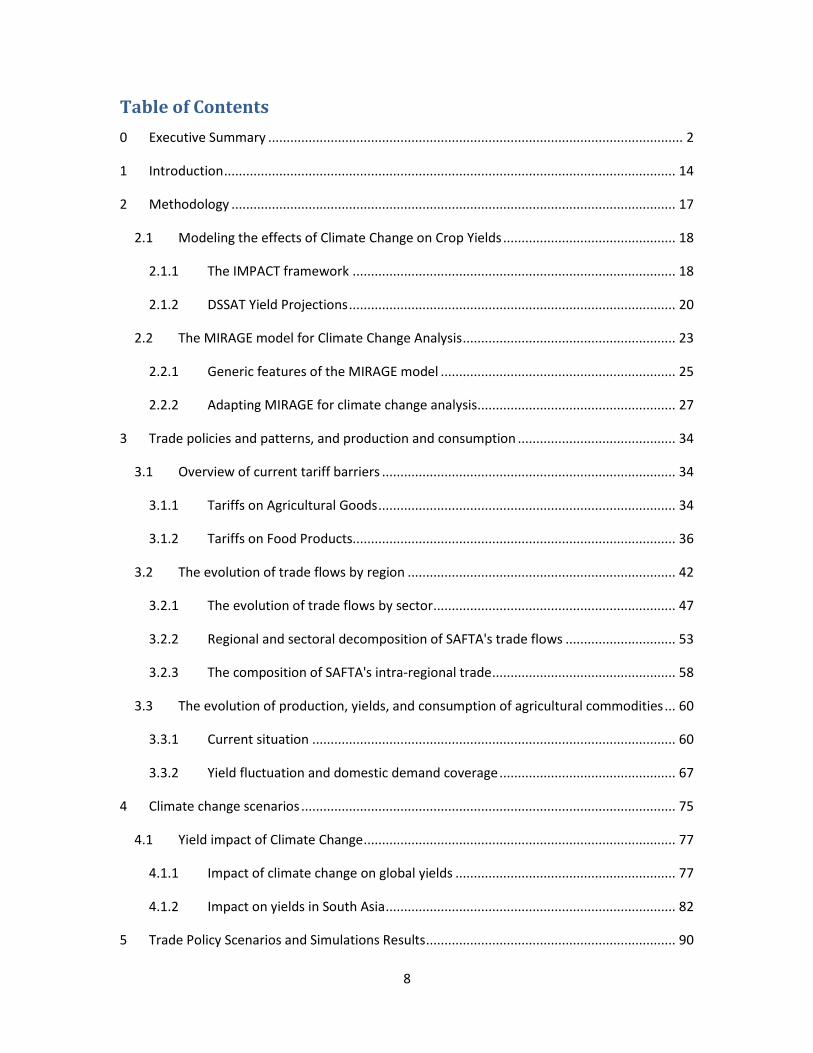
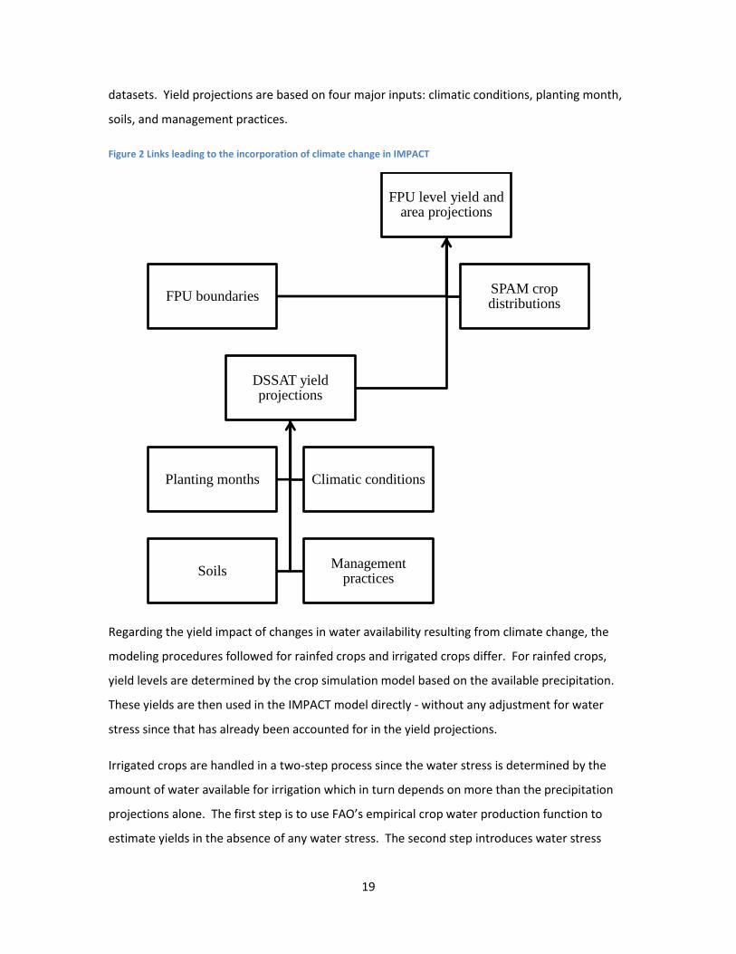
datasets. Yield projections are based on four major inputs: climatic conditions, planting month,

soils, and management practices.

Figure 2 Links leading to the incorporation of climate change in IMPACT

Regarding the yield impact of changes in water availability resulting from climate change, the

modeling procedures followed for rainfed crops and irrigated crops differ. For rainfed crops,

yield levels are determined by the crop simulation model based on the available precipitation.

These yields are then used in the IMPACT model directly - without any adjustment for water

stress since that has already been accounted for in the yield projections.

Irrigated crops are handled in a two-step process since the water stress is determined by the

amount of water available for irrigation which in turn depends on more than the precipitation

projections alone. The first step is to use FAO’s empirical crop water production function to

estimate yields in the absence of any water stress. The second step introduces water stress

FPU level yield and area projections

FPU boundaries SPAM crop distributions

DSSAT yield projections

Planting months Climatic conditions

Soils Management

practices

20

defined by climatic conditions. The stress is introduced through both a hydrologic model and a

water simulation model built into IMPACT. The hydrologic model is a semi-distributed macro-

scale module that covers the entire global land mass (except Antarctica). Based on the

precipitation projections (and other climatic factors), the hydrologic model determines water

availability and potential evapotranspiration under given climatic conditions. The water

simulation model then uses the output of the hydrologic model to determine how much water

would actually be available for irrigation - as compared to how much might be desired.

The economic portion of IMPACT works at a regional level known as the Food Production Unit

(FPU). The biophysical/crop modeling analyses are done in a grid based framework at a much

finer resolution. One of the more challenging aspects of developing the linkages between these

models is dealing with spatial aggregation issues to determine the appropriate typical values

when moving between resolutions. More specifically, the aggregation needs to take yield and

area outputs from the crop modeling process at a fine pixel level to the IMPACT FPUs regional

level.

This is done in the following manner: First, the FPU is chosen along with its geographic

boundary. This is a vector (not a pixel or raster) boundary that encompasses the region and

used to determine which pixels fall within the FPU. Next, the appropriate SPAM data set that

corresponds to the crop/management combination is chosen. The SPAM data come in raster

format, with a spatial resolution of 5 arc-minutes (approximately 10 km at the equator). The

physical area under cultivation in the SPAM data set is used as the weight to calculate the

average yield across the FPU. The areas for the baseline and future years are determined by

adding up the physical areas from SPAM over only the pixels for which it was possible to obtain

yield projections. The total production is computed by taking the SPAM physical area and

multiplying by the projected yield (pixel by pixel) and summing over all locations. The weighted

average yield is then simply calculated as total production divided by total area for the year.

2.1.2 DSSAT Yield Projections

Yield projections are generated using the DSSAT suite of crop simulation modeling tools (DSSAT

2009) on a regular grid covering the surface of the earth. The crop model numerically “grows”

the crop by providing a daily snapshot of how the plant is developing – e.g. number of leaves

that have come out, size of the grains, biomass accumulated etc. The most relevant

characteristic for the IMPACT model is the yield at the end of the season. The data needed to

21

run the crop simulation models can be grouped into four major categories: soil, management

practices, climatic conditions, and planting month (see also Fig. 2 above).

Soil types

DSSAT requires a characterization of the soil properties such as water holding capacity, root

penetration, and nutrient characteristics. This information is needed for several soil layers in

the top two meters of soil. The soil profiles currently used consist of 3×3×3 = 27 generic soil

profiles reflecting high/medium/low fertility, shallow/medium/deep root penetrability, and

sandy/loamy/clay predominant composition. The profiles for each location were assigned based

on interpretation of the FAO harmonized soil maps of the world (FAO 2009, Harmonized World

Soil Database 2009).

Management practices

The management practice category of inputs includes water source, fertilizer application details,

seed choice and planting density. The source of water can be either rainfall or irrigation. With

irrigation, there are several controls that can be specified to reflect how, when, and how much

water is delivered. The amount, type, and timing of fertilizer applications are additional

important considerations. The DSSAT system allows for different varieties or cultivars within

each crop. A major example of this is rice where both japonica and indica varieties are

considered - and separately assigning the results to the geographic locations where each

predominates.

While not a directly controllable management practice, the atmospheric CO2 concentration

would generally fall into this category of inputs. Even though DSSAT has the capability to

consider the CO2 concentration, it is unclear what the effect of CO2 fertilization would actually

be in the field. Additionally, the reliability of its representation in DSSAT is not clear. These

uncertainties led to the choice to run simulations under a “no carbon dioxide fertilization”

assumption where the same value is used in both baseline and future situations for the

atmospheric concentration. This is meant to reflect the case where CO2 fertilization ends up

being inconsequential.

22

Climatic conditions

Climate data are derived from downscaled GCM projections which provide monthly

precipitation, average minimum temperatures, and average maximum temperatures for each

location. Companion downscaling techniques provide the monthly average number of rainy

days and the average incident shortwave solar radiation flux. These techniques are still an area

of active research. The most recent developments and a more detailed description of the

process can be found online at the website listed in the references (Climate Projection Data

Download 2009).

The downscaled datasets are monthly averages, while the crop simulation models work on a

daily time-step requiring daily weather values. One of the tools in the DSSAT suite is a stochastic

weather generator. The generator takes a random seed along with the monthly averages and

generates daily weather profiles that are consistent with the averages using a Monte Carlo

process attuned to weather applications. Since weather is an extremely important determinant

of crop yields, the final yield used for analysis is the mean over the yields resulting from many

weather realizations.

Planting date

Planting date is a critical element of crop management practice. Modeling planting dates on a

global scale has proven to be challenging. Most of the readily available cropping calendar

information is anecdotal and not systematically georeferenced. Attempts have been made to

systematize much of this information into GIS formats (SAGE 2009), but it is still limited by the

underlying sparseness of the data. Furthermore, this information does not provide guidance for

use with future climate scenarios. To address this, rule-based methods were implemented

based on monthly climate data. The baseline rules were calibrated to mimic as closely as

possible the information available from the anecdotal evidence. Comparisons with the SAGE

data have been encouraging. The rules can then be applied to the future climate data to

determine likely planting dates under those conditions.

There are three sets of calendars that have been developed for use with IMPACT so far: general

rainfed crops, general irrigated crops, and spring wheat. For rainfed crops, the idea is to find a

block of months that are not excessively hot, avoid freezing, and have a reasonable amount of

monthly rainfall throughout the block. For those places in the tropics that meet these criteria

23

year-round, the planting month is keyed off of the rainy season. For irrigated crops, the first

choice is the rainfed planting month. When that is unavailable, then a series of special cases are

considered for South Asia, Egypt, and the rest of the northern hemisphere. Otherwise, the

planting month is keyed off of the dry season.

Spring wheat has a complicated set of rules. In the northern hemisphere, the planting month is

based on finding a block of months that are sufficiently warm but not excessively so. If all

months qualify, then the month is keyed off of the dry season. In the southern hemisphere,

spring wheat tends to be grown during the meteorological wintertime as a second crop. Hence,

the planting month does not depend so much on what is optimal for wheat, but rather when the

primary crop is harvested. Hence, the planting date is based on a shift from the rainfed planting

month. Failing that, the planting month is based on the rainy season.

Selected crops

To capture the different capacity of crops to react to climate change, based on their carbon

fixation and photosynthesis capacity, a mix of C3 and C4 plants have been simulated with

DSSAT. Currently, results for all SRES scenarios in the IMPACT framework include groundnut,

maize, rice, soybean and wheat. These crops cover directly, or indirectly, most of the nutritional

needs of animals and humans.

For other crops in the model, simple averages of the relevant C3 or C4 simulated crops based on

the plant category were used. This method is imperfect but at least offers a consistent

framework. In addition, assuming no change in yield for non-simulated crops would be an even

more challenging choice since it would assume that they perfectly adapt to climate change and

will expand strongly. By choosing a simple average, extreme behavior is ruled out and it is

ensured that these crops will follow the main trend.

2.2 The MIRAGE model for Climate Change Analysis

To assess the economy-wide effects of global climate changes, the CGE provides the most

appropriate framework. Climate change modifies agricultural productivity and will have a direct

impact on agricultural commodity prices and factor prices. Through the factor price channels,

factors will be reallocated in the economy and as a result sectoral specialization will change. In

addition, incomes will be affected and demand behavior will be modified. Demand will also be

24

affected by change in prices and food consumption, even if inelastic, will be impacted as well.

Since agricultural products (crops but also fibers and animal products) are important inputs for

many sectors, changes in their prices will affect other sectors. All these channels require the use

of a CGE model that is capable of tracking these changes. In addition, these changes do not

occur in a closed economy but at a global level with heterogeneous effects across countries and

commodities. Comparative advantages evolve, trade patterns adapt and countries are affected

by both the domestic effects of climate change and by the modifications of relative prices in

world markets (terms of trade effects). Over time, considering income and current account

constraints, production will be reallocated across sectors and across regions to adapt to

exogenous changes in yields. Depending on the specific situation, general equilibrium effects

will mitigate or magnify the initial impacts. For example, capital may leave agriculture due to

the negative shock on returns, accelerating the fall in the yields and production levels in one

country; or alternatively may move to this sector attracted by high prices thus compensating, at

least partially, for the exogenous reduction in yields. This is the reason why a multi country,

multi sector, dynamic CGE model is needed. The analysis in this paper uses an upgraded and

adapted version of the MIRAGE model. Below follows a description of the core MIRAGE model

as well as of the modifications that are required to enable to use the model for long term

projections.

In terms of trade analysis, the choice of the Armington assumption (differentiating goods by

country of origin) is important and a major difference when compared with most partial

equilibrium analysis frameworks, including the IMPACT model. The Armington assumption

implies imperfect price transmission between international and domestic markets, and specific

trade patterns at the bilateral level. On the contrary, partial equilibrium assuming perfect

substitution implies a single world market for each agricultural commodity, and unilateral net

trade flows (except for spatial trade models). Nevertheless, while the latter approach has

certain advantages in terms of ease of tracking quantities and simplifying the modeling

framework, the empirical literature (see Villoria 2009 for a recent analysis) strongly argue in

favor of the features that result from adopting the Armington assumption: price transmission is

imperfect, there is no such thing as a single world market, and geography, as well as history,

matter for explaining trade patterns.

25

The sectoral (20 sectors) and regional (20 countries and regions) disaggregations used in this

paper are listed in Table 2 and 3, respectively. They cover the most important trade blocks and

commodities for the purpose of this study. Chapter III provides further justifications for these

choices by discussing trade and production patterns.

Table 2 Sectoral decomposition of the MIRAGE model

Code Sector Description Code Sector Description

cattle Cattle ffl Fossil Fuels coarse Coarse Grains forestry Forestry cotton Cotton omn Other Minerals maize Maize crp Chemical rubbers and plastics oagr Other Ag. Products mmet Mineral and metals oilseed Oilseeds moto Motor vehicles pulses Pulses ome Machinery and equipment rice Rice omf Other manufacture products sugar Sugar p_c Petroleum & coal products veget Vegetables text Textiles wheat Wheat wap Wearing apparel dairymeat Dairy and Meat products wpp Wood and paper products ofood Other Processed Food serv Services vegoils Vegetal Oils trade Trade fishing Fishing trans Transportation

Table 3 Regional decomposition of the MIRAGE model

Code Region Description Code Region Description

ANZCERTA Aus, NZ NAFTA NAFTA

CHN China ARG Argentina

RAS Rest of Asia LAC Latin America

CEA Central Asia BRA Brazil

ASEAN ASEAN CAM Central America

BGD Bangladesh* EU27 EU27

IND India* XER Russia & Ukraine

PAK Pakistan* MED Mediterranean Region

SLK Sri Lanka* WAF Sub Saharan Africa

XAS Rest of South Asia* SAF South Africa

Note: An asterisk * indicates countries/regions belonging to South Asia.

2.2.1 Generic features of the MIRAGE model

MIRAGE is a multi-sector, multi-region Computable General Equilibrium (CGE) model for trade

policy analysis. The model operates in a sequential dynamic recursive way: it is solved for one

period, and then all variable values, determined at the end of a period, are used as the initial

26

values for the next period. Macroeconomic data and social accounting matrixes, in particular,

are derived from the GTAP 7 database (see Narayanan, 2008), which describes the world

economy in 2004. At the supply side, the production function in each sector is a Leontief

function of value-added and intermediate inputs: one output unit needs for its production x

percent of an aggregate of productive factors (labor, unskilled and skilled; capital; land and

natural resources) and (1 – x) percent of intermediate inputs. The intermediate inputs function

is an aggregate CES function of all goods: this means that substitutability exists between two

intermediate goods, depending on the relative prices of these goods. This substitutability is

constant and at the same level for any pair of intermediate goods. Similarly, in the generic

version of the model, value-added is a constant elasticity of substitution (CES) function of

unskilled labor, land, natural resources, and of a CES bundle of skilled labor and capital. This

nesting allows the modeler to introduce less substitutability between capital and skilled labor

than between these two and other factors. In other words, whenever the relative price of

unskilled labor increases, this factor is replaced by a combination of capital and skilled labor,

which are more complementary.1

Factor endowments are fully employed. The only factor whose supply is constant is natural

resources with a few exceptions detailed later. The supply of capital is modified each period

because of depreciation and investment. Growth rates of labor supply are fixed exogenously.

Land supply is endogenous; it depends on the real remuneration of land. In some countries land

is a scarce factor (for example, Japan and the EU) reflected in a low elasticity of supply. In

others (such as Argentina, Australia, and Brazil) land is more abundant and the supply elasticity

is higher.

Skilled labor is the only factor that is perfectly mobile. Installed capital and natural resources

are sector specific. New capital is allocated among sectors according to an investment function.

Unskilled labor is imperfectly mobile between agricultural and nonagricultural sectors according

to a constant elasticity of transformation (CET) function: unskilled labor’s remuneration in

agricultural activities is different to that in nonagricultural activities. This factor is distributed

1 In the generic version, the substitution elasticity between unskilled labor, land, natural resources, and

the bundle of capital and skilled labor is 1.1 - for all sectors except for agriculture where it is equal to 0.1. On the other hand, the substitution elasticity is only 0.6 between capital and unskilled labor.

27

between these two series of sectors according to the ratio of remunerations. Land is also

imperfectly mobile between agricultural sub-sectors.

In the MIRAGE model there is full employment of labor; more precisely, there is a constant

aggregate employment in all countries (wage flexibility). It is quite feasible to assume that total

aggregate employment is variable and that there is unemployment; but this choice greatly

increases the complexity of the model, so that simplifying assumptions have to be made in other

areas (such as the number of countries or sectors). This assumption could amplify the benefits

of trade liberalization for developing countries: in full-employment models, increased demand

for labor (from increased activity and exports) leads to higher real wages, such that the origin of

comparative advantage is progressively eroded; but in models with unemployment, real wages

are constant and exports increases are larger.

Capital (either domestic or foreign) in a given region is assumed to be obtained by combining

intermediate inputs according to a specific combination. The capital good is the same across

sectors. The version of the MIRAGE model used in this paper assumes that all sectors operate

under perfect competition, there are no fixed costs, and prices equal marginal costs.

The demand side is modeled in each region through a representative agent whose propensity to

save is constant. The rest of the national income is used to purchase final consumption.

Preferences between sectors are represented by a linear expenditure system – i.e. constant

elasticity of substitution (LES-CES) function. This implies that consumption has a non-unitary

income elasticity; when consumer’s incomes are augmented by x percent, consumption levels

are not systematically raised by the same percentage, other things being equal. The sectors’

sub-utility functions used in MIRAGE are a nesting of four CES-Armington functions that define

the origin of the goods. In this paper, Armington elasticities are drawn from the GTAP 7

database and are assumed to be identical across regions.

Macroeconomic closure is obtained by assuming that the sum of the balance of goods and

services and foreign direct investments (FDIs) is constant.

2.2.2 Adapting MIRAGE for climate change analysis

To be able to tackle issues related to climate change, the MIRAGE model was modified in several

respects. New crops were introduced, followed by land use modeling to integrate the change in

yields derived from the IMPACT model and adapted to operate at the water basin level,

28

matching the IMPACT FPUs. Finally numerous modifications were performed to reconcile the

dynamic aspect of long term projections.

Introduction of new crops

To consider the heterogeneous effects of climate change on different crops and the important

role of pulses in South Asia diet, two sectors were added to the GTAP7 database: maize and

pulses. The former has been “extracted” from the “other coarse grains” sector while pulses

have been taken from the “vegetable and fruits” GTAP sector. Information on their production

levels was obtained from FAOSTAT. Trade information and tariffs are based on ADEPTA

(Laborde, 2010).

Land use and yield impacts

The first important modification of the MIRAGE model consisted of a breakdown of land

allocation decisions by water basins. Each region / country in the model has a land market

operating at the infra-regional level, mimicking the FPUs in the IMPACT model. Using the FPU

and the underlying river basin decomposition appears to be more robust for climate change

analysis than using agro ecological zones (AEZ) as done in previous studies on medium term land

uses effects (see Al Riffai, Laborde and Dimaranan 2010 for an illustration). Indeed, the AEZ

classification incorporates elements regarding precipitation, water and cropping periods that are

highly endogenous to some of the main issues analyzed in this paper.

The model contains 161 land markets (region times basin) in which producers allocate land

among crops, through a CET function (elasticity of transformation of 0.5 for all basins),

mimicking the standard land supply representation in MIRAGE at the national level. The same

river basin can be shared by several countries. In such cases, markets are segmented by both

the river basin and political borders. Each segment will have its own land price and producers

will take independent decisions. However, crop yield patterns in these differentiated segments

may be correlated due to climatic events. At the national level, all sub-regional land supplies for

a given crop are aggregated through a CET function (with an elasticity of transformation equal to

6) and provide the aggregate land supply for the production function. This large but imperfect

substitution captures the fact that production can be redistributed among different regions of a

country in the long run while respecting biophysical yield.

29

This modeling approach is important for a number of reasons. First and by considering only one

national land market, the yield shifts coming from the crop models need to be aggregated at the

national level using certain weights. Using fixed weights, e.g. the initial area, would fix the link

between geographical distribution of production within a country and yield changes – in other

words would not allow the capture of endogenous reallocation effects. Furthermore, it would

not allow for distinguishing between geographical yield changes and sectoral yield changes. For

the sake of illustration, consider a country with two regions (A and B) and two crops (X and Y).

Yields are initially homogenous. Assume that A & B have the same area and A is specialized at

90 percent in X and B at 90 percent in Y; and that region A is strongly affected by climate change

resulting in a yield decrease of 50 percent, while region B remains unaffected. Operating with a

single land market and importing aggregated yield would lead to the conclusion that production

of crop X and Y decrease by respectively 45 percent and 5 percent. Except in the case of

extremely inelastic demand in a closed economy, substitution effects would dominate and

production factors (such as capital) would flow from X to Y. In addition, since the change in yield

is sector specific and with a standard MIRAGE closure, productivity of land moved from X to Y

would increase. However, this effect is erroneous since the new land taken from X comes from

region A which has lower yields for both crops. With the basin/FPU approach adopted in this

paper, the output from the crop model is expressed by river basin and for each specific crop.

A second important issue is the manner in which irrigation is treated in the model. Irrigation

expenditures or their effects are not modeled in the CGE. Even if agriculture can become more

intensive (more labor and/or capital per unit of land) and physical productivity of land will

increase, this is not necessarily associated with concrete investment projects in physical

infrastructure (irrigation, roads, drainage) or immaterial assets (R&D, new crop varieties). The

IMPACT framework provides the change in yield for irrigated and rainfed crops separately. It is

assumed that the ratio between rainfed and irrigated areas will remain constant for each crop,

and each FPU, for all years and all scenarios. Therefore, an average yield by crop, and its

changes, can be computed for each FPU using the initial ratio between irrigated and rainfed

production. Since irrigation activity is not modeled in the CGE, neither is the water market. A

limitation of this approach is that during expansion of crops that are initially highly irrigated, it is

assumed that the required infrastructure is provided for free, underestimating the real cost of

expansion. However, the problem is only significant when large areas initially occupied by a

rainfed crop are replaced by a strongly irrigated crop. With the lack of representation of the

30

water market and irrigation in the CGE, it also implies that expansion of an irrigated crop will

lead to an incremental demand of water is not considered a scarce resource. In other words,

this increased water demand will not be in competition with other sectors or crops and will not

generate water stress elsewhere.

Finally, it is important to properly model yield shocks. Indeed, the crop models provide

information regarding changes in yield - based on changes in temperature and water availability

- for a defined technology (fertilizers, other inputs) for each period. Therefore, there is a need

to calibrate the model, using the existing technologies (i.e. production functions and elasticities),

the shift in land productivity at the FPU level that will generate for each crop the same change in

physical yield (units produced per unit of land) estimated by the crop model. This procedure is

straightforward since the CES function can be used that defines value added and then rearrange

it to compute a parameter for each FPU and each crop that multiplies the amount of land used

in this sector generating the targeted yield assuming other factors constant. Then, during the

simulations, this parameter is fixed and producers will modify their factor demands to take into

account this factor-specific productivity shifter. This procedure amounts to assuming a non-

neutral productivity shock. Depending on the elasticities in the model, other production factors

can be used to compensate for the productivity loss of land and support production; or

alternatively leave the sector as result of a decline in their marginal productivity (positively

correlated with the exogenous productivity of other factors). For example for capital, new

investment would be avoided resulting in an erosion of the capital stock.

Dynamic perspectives

Projecting the world economy to 2050, in particular when focusing on a fast growing and large

region such as South Asia, is a challenging task that requires adapting the dynamic structure of

MIRAGE as well as making careful choices in terms of baseline assumptions. Dynamic modeling

choices significantly affect the comparative advantage in the baseline since they modify relative

factor endowments in the various economies. The following specific choices were made:

First, the model operates not on a yearly basis but in steps of five years. This solution saves

computational time and since no scenario information is provided with more accuracy - climate

impacts are estimated for 2050 and then backwardly interpolated linearly - there is no gain to

use a yearly frequency. In terms of factor supply, a number of modifications were introduced.

31

Physical investment decisions follow the same behavior as in the standard version of MIRAGE.

No foreign direct investment is allowed. Saving rates in the different economies are not

readjusted since these parameters are impacted by many different mechanisms, some of which

are known (demography) while other remain unknown (future social safety nets, pension

system reform etc.). The only exception in this regard is China that stands as an outlier in the

GTAP database (saving rate exceeding 40 percent) while all other important economies have

savings rates between 15 percent and 25 percent. In the model the saving rate of China is

decreased linearly to 30 percent by 2050 to avoid the explosive investment path that would

otherwise be generated. A more important modification is done for the labor accumulation.

The total number of workers is based on population projections (United Nations data) and an

activity rate (ILO data). The split between skilled and unskilled evolves through a wage gap

equation that is aimed to mimic incentives for education. The ratio between skilled and

unskilled labor of the representative household is an iso-elastic function of the ratio between

the last ten year moving average of skilled labor and unskilled labor. The elasticity has been

calibrated (0.9) for all countries in order to have a meaningful dynamic path in terms of catching

up by developing economies. Finally and to avoid an explosion of natural resource prices,

especially minerals, we consider an iso-elastic supply of natural resources (production factor) in

the mining sector, but not for fossil fuels. All these mechanisms are activated only during the

baseline calibration. These factor supplies remain constant between all alternative trade policy

baselines and climate change scenarios.

In terms of demand, two modifications were made to the standard MIRAGE model. First and

regarding final demand, a dynamic recalibration of the CES – LES was introduced which aims to

capture the evolution of the standard of living. Indeed without such a dynamic recalibration,

the CES LES displays an increase in the price elasticity for countries where the rise in income has

brought current levels of consumption, in particular for food products, far from their base levels.

The dynamic recalibration allows to redefine the minimum per capita consumption of the CES

LES and the elasticity of substitution, between each period in order to remain as close as

possible to the targeted income and price elasticity for each commodity and region. This

recalibration is only performed in the baseline and temporal values of parameters are used in

the simulations. This allows maintaining the same preference structure between the baseline

and the simulations, as well as performing welfare analysis. Second, an energy efficiency

parameter on the use of fossil fuels (oil and natural gas) was introduced. This parameter was

32

calibrated and applied homogenously on all demand, to reproduce the IEA energy price

projections.

Finally, to avoid explosion of cumulated current account imbalances, all current accounts were

forced to converge to zero by 2050. Consequently, in each country the real exchange rate

adjusts endogenously to adjust the trade balance.

In addition to the other dynamic calibration steps described above, additional assumptions and

mechanisms were introduced that allow building a dynamic baseline. The main target is a GDP

growth based on World Bank projections as used in the central scenario of IMPACT long term

projections (see Nelson et al., 2010). With the total labor force treated as exogenous

(population and activity rate assumptions), endogenous capital accumulation and endogenous

skilled / unskilled labor ratios, the model has only one degree of freedom by region to reach the

GDP target: the total factor productivity (TFP) for all sectors and factors. Therefore calibration

was performed endogenously following normal MIRAGE procedures. However, if this TFP is

applied to all factors, agricultural yields will grow quite fast, especially in India. Therefore, this

TFP was adjusted with an agriculture-specific TFP that reduces the generic term. This additional

term is country and sector specific and is freed during the calibration stage to target the

(exogenous) growth rate of physical yield in agriculture based on the IMPACT baseline that

provides detailed assumption for different crops and regions.

Using this procedure, a dynamic baseline was constructed that exhibits a number of desirable

features: evolution of the economic size of the different regions (GDP), per capita income,

relative prices between factors, relative productivity between sectors etc. Finally, it is important

to note three additional characteristics of the model. First, the baseline is independent of the

SRES scenarios in terms of emissions. Indeed, the same GDP growth can be achieved through

very different technological pathways in terms of GHG effects. Second, the calibration process

is implemented with a status quo assumption in terms of trade policy. This paper includes

different trade policy options to study the role of the trade environment on the consequences

of climate change. However, these trade policy modifications are implemented in the last stage

of the baseline, during the policy pre-experiment and not during the calibration stage. This

implies that while the GDP of countries will change between alternative trade policy baselines,

the TFP remains constant. Finally, demand of agricultural feedstock for biofuels is not taken into

account. Instead it is assumed that first-generation biofuels, and potentially the second

33

generation, will be phased out by 2050 and that bioenergy programs will not lead to increased

pressure on agricultural land.

34

3 Trade policies and patterns, and production and consumption

3.1 Overview of current tariff barriers2

This section provides a short overview of the structure of current tariff barriers in SAFTA

countries. Subsequent subsections describe the structure of protection on agricultural goods in

general, followed by a focus on food products and the structure of tariffs according to

respectively calorie, protein and fat contents of trade.

SAFTA countries have highly restrictive trade policies - tariffs applied on their imports are about

twice as high as the tariffs faced by their exports in 2006 (Bouet and Corong, 2009). Non-food

tariff barriers are the highest in Bangladesh while on the other extreme Sri Lanka's average

industrial protection rates do not exceed 7 percent. Tariffs on textiles and wearing apparel are

high in Bangladesh (30 percent) and Pakistan (24 percent) while Sri Lanka's tariffs in this sector

are the lowest among SAFTA countries. Whereas Sri Lanka is the least protectionist among the

SAFTA countries, India has by far the most protectionist trade regime – with an average tariff on

ag-food imports of 58 percent and even higher tariffs on rice imports (80 percent) and on

imports of wheat and processed sugar (100 percent). Note that despite the preferential access

granted by India to other SAFTA countries, tariff barriers are still high.

3.1.1 Tariffs on Agricultural Goods

SAFTA as a whole3 applies higher tariff rates on imported agricultural products from the rest of

the world (47.3 percent on average) than the tariff rates faced by SAFTA's agricultural exports

(23.9 percent on average). Average tariff rates applied on agricultural imports from the main

continents are fairly even: North American products face the highest import tariffs (52.2

percent), followed by European and South American products (49.7 percent each). On the other

hand, SAFTA's agricultural exports face the highest average import tariffs in Asia & Oceania (29.7

percent) and the lowest in North America (9.2 percent). These results are consistent with global

2 This section focuses on tariff barriers. Indeed, they are the primary policy instrument used in the model

scenarios. However, agricultural trade in South Asia is also subject to a wide array of non-tariff barriers and export policies (subsidies or restrictions based on conjectural needs). The distortive role of these policies should not be neglected as well as the potential for further trade liberalization that they represent. 3 Weighted average - SAFTA figures are largely driven by Indian policies.

35

protection patterns and do not display any sign of negative discrimination. Note that intra-

regional tariff rates among SAFTA member countries still pertain (13.7 percent in agriculture) –

mainly because a number of sensitive products (negative list) are excluded from full

liberalization under SAFTA's free trade agreement.

Among SAFTA's member countries, India applies the highest rates of protection on agricultural

products (62.7 percent), compared to 13 percent in Bangladesh which is the least protective

among SAFTA members. Interestingly, it is the LDC (Least Developed Countries) member

countries of SAFTA such as Maldives, Nepal and Pakistan that are relatively less protectionist

with respect to their agricultural imports originating from the rest of the world - their tariff rates

applied on imported agricultural products are lower than the tariffs faced by their agricultural

exports (see Figure 3).

36

Figure 3 Average Tariffs on Agricultural products in 2007 for South Asian countries (Reference group weighted)

Source: ADEPTA database (Laborde, 2010). Authors' computations.

3.1.2 Tariffs on Food Products

Average protection levels applied to imports and faced by exports of food products of SAFTA

countries do not differ all that much from those of agricultural commodities (Figure 4).

Nevertheless, average import tariffs on food imports of SAFTA are 4 percentage points higher

(51.1 percent) than average import tariffs on agricultural commodities, while in the rest of the

world food exports of SAFTA face slightly higher barriers (25.1 percent) than agricultural

products. Once again, India is the most protectionist country regarding food imports with 65.6

percent average tariff rates - and even higher tariffs (71.1 percent) on food imports originating

from Asia & Oceania. Note that among the highest tariffs applied on exports of SAFTA countries

65 55 45 35 25 15 5 5 15 25 35 45 55 65

World

SAFTA partners

Asia & Oceania

Africa

Europe

North America

South America

World

SAFTA partners

Asia & Oceania

Africa

Europe

North America

South America

World

SAFTA partners

Asia & Oceania

Africa

Europe

North America

South America

World

SAFTA partners

Asia & Oceania

Africa

Europe

North America

South America

SAFT

AB

angl

ades

hB

hu

tan

Ind

ia

Tariffs Applied on Imports Tariff faced on exports

65 55 45 35 25 15 5 5 15 25 35 45 55 65

World

SAFTA partners

Asia & Oceania

Africa

Europe

North America

South America

World

SAFTA partners

Asia & Oceania

Africa

Europe

North America

South America

World

SAFTA partners

Asia & Oceania

Africa

Europe

North America

South America

World

SAFTA partners

Asia & Oceania

Africa

Europe

North America

South America

Mal

div

esN

epal

Pak

ista

nSr

i lan

ka

Tariffs Applied on Imports Tariff faced on exports

37

are those in European countries which apply an average 73.1 percent tariff on food imports

from Nepal.

Figure 4 Average Tariffs on Food products for South Asian countries (Reference group weighted)

Source: ADEPTA database (Laborde, 2010). Authors' computation.

Note that the average tariff levels discussed above are computed using a trade value weighted

scheme. While average tariffs provide key messages in terms of overall economic distortions, it

is difficult to draw conclusions in terms of the nutritional consequences of these trade barriers.

100 80 60 40 20 0 20 40 60 80 100

World

SAFTA partners

Asia & Oceania

Africa

Europe

North America

South America

World

SAFTA partners

Asia & Oceania

Africa

Europe

North America

South America

World

SAFTA partners

Asia & Oceania

Africa

Europe

North America

South America

World

SAFTA partners

Asia & Oceania

Africa

Europe

North America

South America

SAFT

AB

angl

ades

hB

hu

tan

Ind

ia

Tariffs Applied on Imports Tariff faced on exports

100 80 60 40 20 0 20 40 60 80 100

World

SAFTA partners

Asia & Oceania

Africa

Europe

North America

South America

World

SAFTA partners

Asia & Oceania

Africa

Europe

North America

South America

World

SAFTA partners

Asia & Oceania

Africa

Europe

North America

South America

World

SAFTA partners

Asia & Oceania

Africa

Europe

North America

South America

Mal

div

esN

epal

Pak

ista

nSr

i lan

ka

Tariffs Applied on Imports Tariff faced on exports

38

Therefore Figure 5, Figure 6 and Figure 7 below provide a decomposition of average tariff rates

using as weights the calorie, fat and protein content of trade, respectively.4

Figure 5 Average Tariffs on Calories for South Asian countries

Source: ADEPTA database (Laborde, 2010). Authors' computation.

Figure 5 shows that overall across SAFTA members and their trading partners, average tariff

levels faced by SAFTA's exports weighted by the calorie content of trade are relatively low (10.7

percent). Notable exceptions include tariff rates faced by exports of calories of Nepal to Europe

4 Note that while average tariffs on agriculture and food have been built using the reference group weight

(Laborde, 2010), in the case tariffs on calories, fats and proteins the bilateral trade nutritional contents weighting scheme has been applied. Given the different weighting schemes, one cannot directly compare average protection rates in agriculture and food with that of calories, fats and proteins.

100 80 60 40 20 0 20 40 60 80 100

World

SAFTA partners

Asia & Oceania

Africa

Europe

North America

South America

World

SAFTA partners

Asia & Oceania

Africa

Europe

North America

South America

World

SAFTA partners

Asia & Oceania

Africa

Europe

North America

South America

World

SAFTA partners

Asia & Oceania

Africa

Europe

North America

South America

SAFT

AB

angl

ades

hB

hu

tan

Ind

ia

Tariffs Applied on Imports Tariff faced on exports

100 80 60 40 20 0 20 40 60 80 100

World

SAFTA partners

Asia & Oceania

Africa

Europe

North America

South America

World

SAFTA partners

Asia & Oceania

Africa

Europe

North America

South America

World

SAFTA partners

Asia & Oceania

Africa

Europe

North America

South America

World

SAFTA partners

Asia & Oceania

Africa

Europe

North America

South America

Mal

div

esN

epal

Pak

ista

nSr

i lan

ka

Tariffs Applied on Imports Tariff faced on exports

39

(126.1 percent) due to the role of sugar exports and the regime of tariff rate quotas which was

still in effect in 2007; and the exports of Bhutan to remaining SAFTA member countries (45.1

percent). On the other hand, average tariffs applied on imports by SAFTA countries weighted by

calorie content of trade (38.2 percent on average) are dominated by the high tariffs of India and

Bhutan. More specifically, India applies a 76.4 percent tariff rate on calorie imports from the

rest of the world, and an even higher rate (87.1 percent) on calorie imports originating from

Asian & Oceania. High tariffs on calorie imports in India are a particular burden for the poor

who spend a large proportion of their income on calorie-rich foods.

Figure 6 Average Tariffs on Fats for South Asian countries

Source: ADEPTA database (Laborde, 2011). Authors' computation.

100 80 60 40 20 0 20 40 60 80 100

World

SAFTA partners

Asia & Oceania

Africa

Europe

North America

South America

World

SAFTA partners

Asia & Oceania

Africa

Europe

North America

South America

World

SAFTA partners

Asia & Oceania

Africa

Europe

North America

South America

World

SAFTA partners

Asia & Oceania

Africa

Europe

North America

South America

SAFT

AB

angl

ades

hB

hu

tan

Ind

ia

Tariffs Applied on Imports Tariff faced on exports

100 80 60 40 20 0 20 40 60 80 100

World

SAFTA partners

Asia & Oceania

Africa

Europe

North America

South America

World

SAFTA partners

Asia & Oceania

Africa

Europe

North America

South America

World

SAFTA partners

Asia & Oceania

Africa

Europe

North America

South America

World

SAFTA partners

Asia & Oceania

Africa

Europe

North America

South America

Mal

div

esN

epal

Pak

ista

nSr

i lan

ka

Tariffs Applied on Imports Tariff faced on exports

40

Average tariff rates weighted by the fat content of trade are slightly higher than when weighted

by calories (Figure 6). On the one hand, SAFTA applies an average 44.4 percent tariff rate on fat

imports (4.2 percent higher than for calorie imports). India again proves to be the most

protectionist country in South Asia, with an average tariff rate on fat imports of 76.9 percent,

followed by Bhutan with 43.9 percent. On the other hand, fat exports of SAFTA to the rest of

the world face an average tariff of 12.6 percent, or only 1.9 percent higher than that on calories.

The highest average tariffs on fats are applied to exports of Bhutan (45 percent). This high

import duty is mainly defined by the high protection rate applied on Bhutan's exports to other

SAFTA member countries (45.2 percent) - an indication that the fact that Bhutan's exports to

other SAFTA members are intensive in fat content while the list of sensitive products is

dominated by products with high fat content.

41

Figure 7 Average Tariffs on Proteins for South Asian countries

Source: ADEPTA database (Laborde, 2011). Authors' computation.

When compared to calories and fats, proteins have the lowest import duties across SAFTA

member countries and their trading partners (see Figure 7). Average tariffs applied on imports

of proteins are only about half of those applied on fats, i.e. 22.2 percent for SAFTA as a whole,

while average tariffs faced by the exports of proteins of SAFTA are similarly lower (5.4 percent

overall).

In summary, the structure of protection applied on imports to SAFTA countries is mainly

dominated by high tariffs in India and Bhutan. LDC member countries of SAFTA are less

protective towards their imports than other SAFTA members, and in addition tend to apply

100 80 60 40 20 0 20 40 60 80 100

World

SAFTA partners

Asia & Oceania

Africa

Europe

North America

South America

World

SAFTA partners

Asia & Oceania

Africa

Europe

North America

South America

World

SAFTA partners

Asia & Oceania

Africa

Europe

North America

South America

World

SAFTA partners

Asia & Oceania

Africa

Europe

North America

South America

SAFT

AB

angl

ades

hB

hu

tan

Ind

ia

Tariffs Applied on Imports Tariff faced on exports

100 80 60 40 20 0 20 40 60 80 100

World

SAFTA partners

Asia & Oceania

Africa

Europe

North America

South America

World

SAFTA partners

Asia & Oceania

Africa

Europe

North America

South America

World

SAFTA partners

Asia & Oceania

Africa

Europe

North America

South America

World

SAFTA partners

Asia & Oceania

Africa

Europe

North America

South America

Mal

div

esN

epal

Pak

ista

nSr

i lan

ka

Tariffs Applied on Imports Tariff faced on exports

42

lower protection levels on their imports compared to protection levels faced by their exports.

Average protection rates that pertain among SAFTA member countries indicate that the list of

sensitive products is intensive in fat and calorie content, but less so in protein content.

3.2 The evolution of trade flows by region

Figure 8, Figure 9 and Figure 10 describe the evolution of trade flows of SAFTA decomposed by

respectively major geographical partners and calorie, protein and fat content. This

decomposition of trade flows by nutritional content compared to the more traditional

decomposition in value terms is essential in determining the role of trade in food security.

A number of clear patterns emerge. First and in line with the gravity model of trade, variables

such as geographical distance, trade costs or preferences highly influence trade patterns – as a

result intra-regional trade and trade with relatively close neighbors (rest of Asia, Australia and

New Zealand) represent a significant share of total trade. Second, Africa is an important

destination market for SAFTA ag-food exports. Last and not surprisingly, the Americas (North

and South) are net exporters of ag-food products to SAFTA given their strong comparative

advantage in producing such products. Thus, geography matters which justifies the use of the

Armington assumption (Armington, 1969) in the CGE model (Hertel and Villoria, 2009).

SAFTA as a whole has been a net importer of calories throughout the 1997 – 2007 period (see

Figure 8 - 1996 is an exception). During that period, the share of imports of calories in total

trade has increased faster than the share of calorie exports. The overall trade balance with

respect to calories deteriorated from 1997 to 1999, then improved slightly until 2004 and

followed by a further deterioration until 2007. Exports of calories have approximately doubled

from 62,227 billion in 1996 to 102,628 billion in 2007, while imports of calories have increased

more than three-fold from 59,244 billion in 1996 to 175,249 billion during the same period. In

per capita terms, the evolution of trade balances follows the general trend in the sense that the

increase of imports is not so much due to a population increase but rather the result of

increases in income and/or competitiveness of imports.

Asian & Oceania is SAFTA’s most significant trading partner, accounting for 50 percent of total

caloric exports of SAFTA in 2007 and 64 percent of caloric imports. Other significant export

markets are SAFTA's intra-regional market and Europe. While Africa in 2007 accounted for 15

percent of caloric exports of SAFTA, its share in total imports of calories of SAFTA is insignificant.

43

On the other hand, while imports of calories from North America and South America accounted

for about 10 percent each of SAFTA’s total caloric imports in 2007, these regions are not

important markets for SAFTA's caloric exports.

During the period 1996-2007 SAFTA was a net protein exporter (Figure 9). Exports of proteins

increased from 3,447 kilotons in 1996 to 4,770 kilotons in 2007, while imports grew from 1,015

kilotons in 1996 to 4,264 kilotons in 2007. As in the case of trade of calories, Asia & Oceania is

SAFTA’s most important protein trade partner - accounting for 73 percent of total protein

exports and 49 percent of total protein imports in 2007. North America is the second largest

import market (accounting for 20 percent of SAFTA’s total protein imports in 2007) but not a

significant export market; Africa is the third largest export market (accounting for 6 percent of

SAFTA’s total protein exports in 2007) but not an important import market for proteins.

The SAFTA region is a net fat importer (Figure 10). Between 1996 and 2007 fat exports

approximately doubled (from 991 kilotons to 1,865 kilotons) but fat imports increased three-

fold (from 3,754 kilotons in 1996 to 10,142 kilotons in 2007). Europe and SAFTA's intra-regional

markets are important export destinations, while North and South America are significant

sources of SAFTA's fat imports.

To conclude, SAFTA is a net importer of calories and fats and a net exporter of proteins. Asia &

Oceania constitutes by far the most important export and import market for SAFTA's exports

and imports of calories, proteins and fats. North and South America are important import

markets but their share in total exports of SAFTA is small. Africa on the other hand is an

important export market, but not an important source of imports. Finally, the regional

decomposition of trade has stayed rather constant over time.

44

Figure 8 Exports and Imports of Calories by Region (billions)

Note: Upper graph is exports, lower graph is imports.

-

20,000

40,000

60,000

80,000

100,000

120,000

140,000

160,000

180,000

200,000

1996 1997 1998 1999 2000 2001 2002 2003 2004 2005 2006 2007

-

20,000

40,000

60,000

80,000

100,000

120,000

140,000

160,000

180,000

200,000

1996 1997 1998 1999 2000 2001 2002 2003 2004 2005 2006 2007

Asia & Oceania (none SAFTA) South America North America SAFTA Europe Africa

45

Figure 9 Exports and Imports of Proteins by Region (kilotons)

Note: Upper graph is exports, lower graph is imports.

-

1,000

2,000

3,000

4,000

5,000

6,000

1996 1997 1998 1999 2000 2001 2002 2003 2004 2005 2006 2007

-

1,000

2,000

3,000

4,000

5,000

6,000

1996 1997 1998 1999 2000 2001 2002 2003 2004 2005 2006 2007

Asia & Oceania (none SAFTA) North America SAFTA Europe South America Africa

46

Figure 10 Exports and Imports of Fats by Region (kilotons)

Note: Upper graph is exports, lower graph is imports.

-

200

400

600

800

1,000

1,200

1,400

1,600

1,800

2,000

1996 1997 1998 1999 2000 2001 2002 2003 2004 2005 2006 2007

-

2,000

4,000

6,000

8,000

10,000

12,000

1996 1997 1998 1999 2000 2001 2002 2003 2004 2005 2006 2007

Asia & Oceania (none SAFTA) South America North America Europe SAFTA Africa

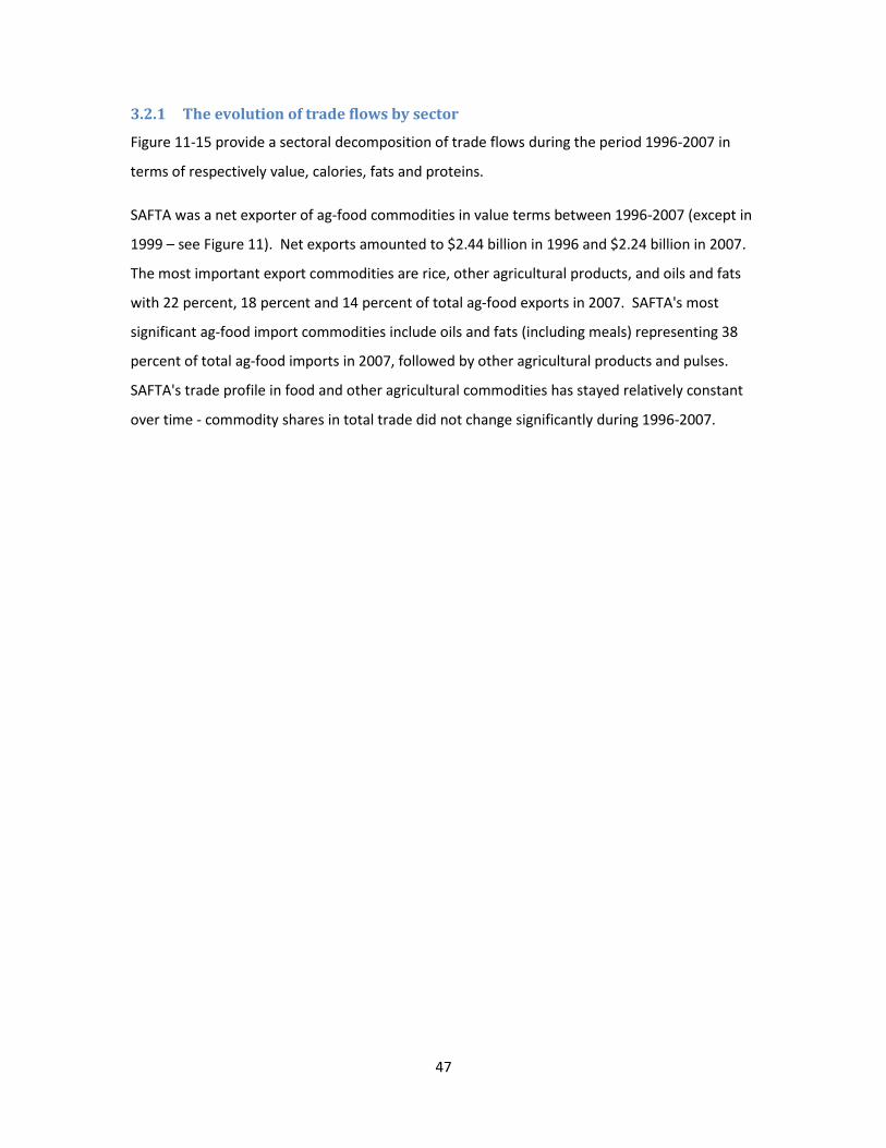
47

3.2.1 The evolution of trade flows by sector

Figure 11-15 provide a sectoral decomposition of trade flows during the period 1996-2007 in

terms of respectively value, calories, fats and proteins.

SAFTA was a net exporter of ag-food commodities in value terms between 1996-2007 (except in

1999 – see Figure 11). Net exports amounted to $2.44 billion in 1996 and $2.24 billion in 2007.

The most important export commodities are rice, other agricultural products, and oils and fats

with 22 percent, 18 percent and 14 percent of total ag-food exports in 2007. SAFTA's most

significant ag-food import commodities include oils and fats (including meals) representing 38

percent of total ag-food imports in 2007, followed by other agricultural products and pulses.

SAFTA's trade profile in food and other agricultural commodities has stayed relatively constant

over time - commodity shares in total trade did not change significantly during 1996-2007.

48

Figure 11 Exports and Imports by Sectors in 103 US dollars

Note: Upper graph is exports, lower graph is imports.

Figure 12 illustrates the evolution of SAFTA's ag-food commodity trade decomposed by the

calorie content of these sectors. Oils and fats are the most significant source of caloric imports

accounting for 44 percent of the total (compared to 38 percent of total import value), followed

by wheat with a 30 percent share. As far as caloric exports are concerned, rice has the highest

0

2,000,000

4,000,000

6,000,000

8,000,000

10,000,000

12,000,000

14,000,000

16,000,000

18,000,000

1996 1997 1998 1999 2000 2001 2002 2003 2004 2005 2006 2007

0

2,000,000

4,000,000

6,000,000

8,000,000

10,000,000

12,000,000

14,000,000

16,000,000

18,000,000

1996 1997 1998 1999 2000 2001 2002 2003 2004 2005 2006 2007

Oils and Fats Other Agric. Products Pulses

wheat Sugar Fruits & Vegetables

Oth. Processed Foods Dairy & Meat products Oilseeds

Rice cattle Maize

Other Coarse grains Fishing

49

share in the total (32 percent as compared to a 22 percent share in total export value). Whereas

the “other agricultural products” sector accounts for 18 percent of the value of total ag-food

exports of SAFTA, its share in total exports of calories is insignificant.

Figure 12 Exports and Imports of Calories by Sector (103 metric tons)

Note: Upper graph is exports, lower graph is imports.

-

20,000

40,000

60,000

80,000

100,000

120,000

140,000

160,000

180,000

200,000

1996 1997 1998 1999 2000 2001 2002 2003 2004 2005 2006 2007

-

20,000

40,000

60,000

80,000

100,000

120,000

140,000

160,000

180,000

200,000

1996 1997 1998 1999 2000 2001 2002 2003 2004 2005 2006 2007

Oils and Fats wheat Sugar

Pulses Oilseeds Rice

Oth. Processed Foods Dairy & Meat products Fruits & Vegetables

Maize Other Agric. Products Other Coarse grains

cattle Fishing

50

Exports of oils and fats account for the highest share (68 percent - see Figure 13) of total exports

of proteins (largely because oilseed meals are included in this sector) but represent only 14

percent of total exports in value terms (and 10 percent of total protein imports because

exported oils and fats are higher in protein content that imports). The share of wheat in total

protein exports increased between 1998 and 2002 (21 percent of total protein exports in 2002

compared to 1 percent in 1998), an increase commensurate with the increase in value of wheat

exports during the same period period. Wheat and pulses are the most important sources of

imported proteins, representing respectively 45 percent and 20 percent of total imports of

proteins in 2007.

Figure 14 describes the sectoral composition of SAFTA’s exports and imports of fats. Oils & fats

and oilseeds are clearly the two most important sources of fats in total trade, accounting for

respectively 56 percent and 16 percent of total exports of fats in 2007, and respectively 86

percent and 6 percent of total imports of fats.

51

Figure 13 Exports and Imports of Proteins by Sector (103 metric tons)

Note: Upper graph is exports, lower graph is imports.

-

1,000

2,000

3,000

4,000

5,000

6,000

1996 1997 1998 1999 2000 2001 2002 2003 2004 2005 2006 2007

-

1,000

2,000

3,000

4,000

5,000

6,000

1996 1997 1998 1999 2000 2001 2002 2003 2004 2005 2006 2007

wheat Pulses Oils and Fats

Oilseeds Dairy & Meat products Oth. Processed Foods

Rice Fruits & Vegetables Maize

Other Agric. Products cattle Other Coarse grains

Sugar Fishing

52

Figure 14 Exports and Imports of Fats by Sector (103 metric tons)

Note: Upper graph is exports, lower graph is imports.

-

200

400

600

800

1,000

1,200

1,400

1,600

1,800

2,000

1996 1997 1998 1999 2000 2001 2002 2003 2004 2005 2006 2007

-

2,000

4,000

6,000

8,000

10,000

12,000

1996 1997 1998 1999 2000 2001 2002 2003 2004 2005 2006 2007

Oils and Fats Oilseeds Dairy & Meat products

wheat Fruits & Vegetables Pulses

Oth. Processed Foods Other Agric. Products Maize

Rice cattle Other Coarse grains

Sugar Fishing

53

3.2.2 Regional and sectoral decomposition of SAFTA's trade flows

Figure 15-18 display a decomposition of trade flows in terms of value, calories, proteins and fats

- this time simultaneously by region and by sector.

Figure 15 represents exports and imports of ag-food commodities in value terms. Asia &

Oceania is SAFTA's most significant trading partner. For example it is the origin of 70 percent of

SAFTA's imports of oils and fats, and the destination for 67 percent of SAFTA's exports of other

coarse grains. Another significant export and import market is represented by SAFTA's intra-

regional market, in particular in the case of sugar (62 percent of total sugar exports) and maize

(66 percent of total imports). South America is not a significant market for SAFTA's ag-food

exports, even though it is an important source of sugar imports (38 percent of SAFTA’s total

imports of sugar).

Note: Upper graph is exports, lower graph is imports.

Figure 16 provides an overview of the composition of trade of calories by ag-food sector and

trading partners. Again Asia & Oceania comes to bear as an important source and destination

for SAFTA’s trade in ag-food products. For example and when expressed in calorie terms, Asia &

Oceania is the destination of 73 percent of SAFTA’s total cattle exports and 69 percent of its oils

and fats exports. When expressed in calorie terms, SAFTA sources respectively 90 percent and

84 percent of its rice and maize imports from inside the region.

The composition of SAFTA's trade flows by fat and protein content split out by region are

presented in respectively Figure 13 and Figure 14.

54

Figure 15 Composition of Exports and Imports (value)

Note: Upper graph is exports, lower graph is imports.

0% 10% 20% 30% 40% 50% 60% 70% 80% 90% 100%

Rice

Oth. Agric.

Oth. Processed Foods

Oils and Fats

Dairy & Meat products

Fruits & Vegetables

Sugar

Oilseeds

Pulses

wheat

cattle

Maize

Other Coarse grains

Fishing

0% 10% 20% 30% 40% 50% 60% 70% 80% 90% 100%

Oils and Fats

Oth. Agric.

Pulses

wheat

Sugar

Fruits & Vegetables

Oth. Processed Foods

Dairy & Meat products

Oilseeds

Rice

cattle

Maize

Other Coarse grains

Fishing

Africa Asia (none SAFTA) & Oceania Europe North America South America SAFTA

55

Figure 16 Composition of Exports and Imports of Calories

Note: Upper graph is exports, lower graph is imports.

0% 10% 20% 30% 40% 50% 60% 70% 80% 90% 100%

Rice

Oils and Fats

Sugar

Oth. Processed Foods

wheat

Oilseeds

Maize

Oth. Agric.

Pulses

Dairy & Meat products

Fruits & Vegetables

Other Coarse grains

cattle

Fishing

0% 10% 20% 30% 40% 50% 60% 70% 80% 90% 100%

Oils and Fats

wheat

Sugar

Pulses

Oilseeds

Rice

Oth. Processed Foods

Fruits & Vegetables

Dairy & Meat products

Oth. Agric.

Maize

Other Coarse grains

cattle

Fishing

Africa Asia (none SAFTA) & Oceania Europe North America South America SAFTA

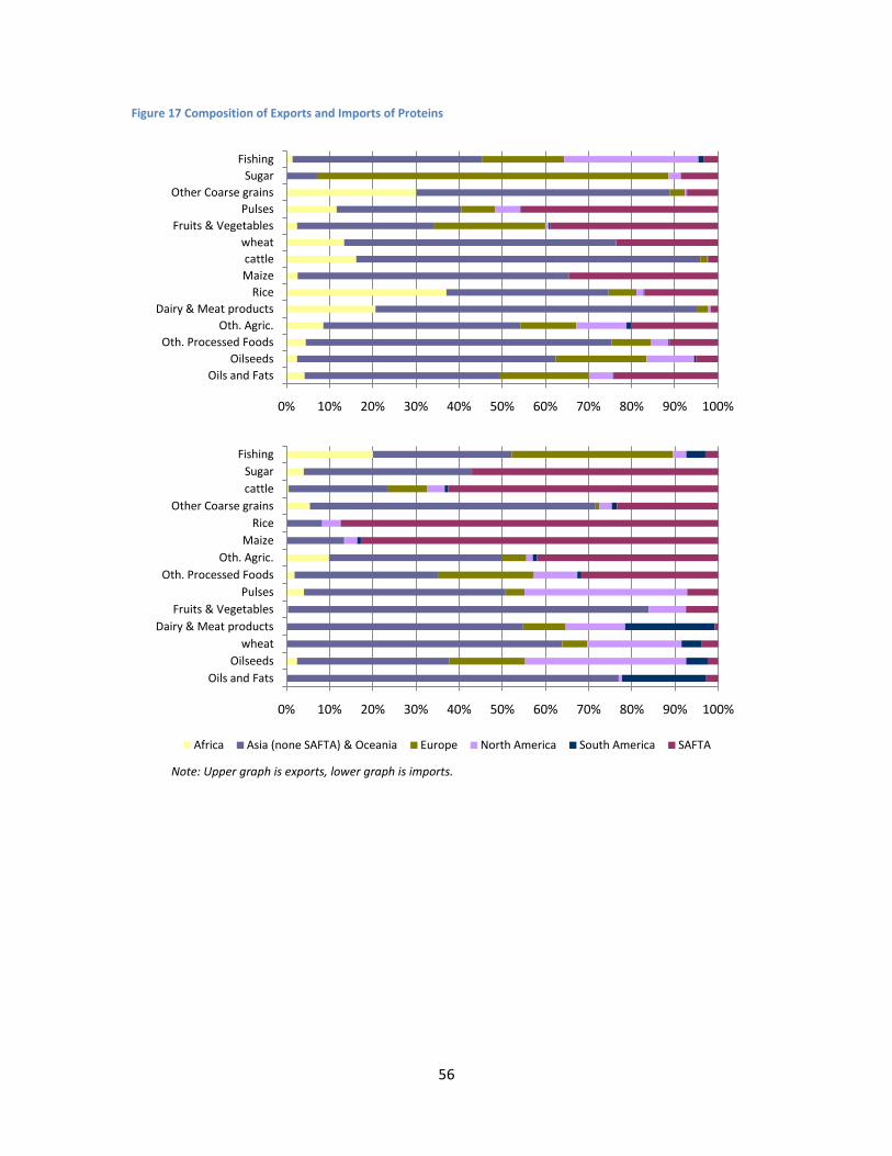
56

Figure 17 Composition of Exports and Imports of Proteins

Note: Upper graph is exports, lower graph is imports.

0% 10% 20% 30% 40% 50% 60% 70% 80% 90% 100%

Oils and Fats

Oilseeds

Oth. Processed Foods

Oth. Agric.

Dairy & Meat products

Rice

Maize

cattle

wheat

Fruits & Vegetables

Pulses

Other Coarse grains

Sugar

Fishing

0% 10% 20% 30% 40% 50% 60% 70% 80% 90% 100%

Oils and Fats

Oilseeds

wheat

Dairy & Meat products

Fruits & Vegetables

Pulses

Oth. Processed Foods

Oth. Agric.

Maize

Rice

Other Coarse grains

cattle

Sugar

Fishing

Africa Asia (none SAFTA) & Oceania Europe North America South America SAFTA

57

Figure 18 Composition of Exports and Imports of Fats

Note: Upper graph is exports, lower graph is imports.

0% 10% 20% 30% 40% 50% 60% 70% 80% 90% 100%

Oils and Fats

Rice

Oth. Processed Foods

wheat

Dairy & Meat products

Oilseeds

Pulses

Maize

Oth. Agric.

cattle

Fruits & Vegetables

Other Coarse grains

Fishing

Sugar

0% 10% 20% 30% 40% 50% 60% 70% 80% 90% 100%

wheat

Pulses

Oils and Fats

Oilseeds

Dairy & Meat products

Oth. Processed Foods

Rice

Fruits & Vegetables

Oth. Agric.

Maize

Other Coarse grains

cattle

Fishing

Sugar

Africa Asia (none SAFTA) & Oceania Europe North America South America SAFTA

58

3.2.3 The composition of SAFTA's intra-regional trade

Table 4-6- provide an overview of SAFTA's intra-regional trade weighted by the calorie, protein

and fat content of trade respectively. We find that India is by far the most significant trading

partner of all other SAFTA countries. Bhutan and Nepal only import from India and Pakistan,

while all SAFTA member countries export to Bangladesh, India and Pakistan.

In calorie terms (see Table 4), while India accounts for 78 percent of intra-regional exports of

calories, its share of total intra-regional imports is significantly lower at 19 percent. This finding

is consistent with the structure of average protection rates described above: the average tariff

level applied by India on imports of calories originating from the rest of SAFTA is 9.1 percent,

compared to a 4 percent average tariff faced by Indian exports.

India is the destination of 99 percent of Nepal's exports, 93 percent of Bangladesh's and 92

percent of Sri Lanka’s. On the other hand, India's most significant regional export markets

include Bangladesh (48 percent of total intra-regional caloric exports), Sri Lanka (20 percent) and

Pakistan (20 percent). This order changes when it comes to India's imports of calories: Sri Lanka

accounts for 40 percent of India's total caloric imports, followed by Nepal (27 percent) and

Pakistan (23 percent).

With respect to trade values weighted by the protein content (Table 5) and fat content of trade

(Table 6), the composition of trade does not change significantly when compared to that of

calories. However, India's imports from Sri Lanka are less intensive in protein content than

calorie content - but more intensive in fat content than in both calorie and protein content.

Table 4 Bilateral Exports of Calories (106 metric tons)

Importer/

Exporter

Bangladesh Bhutan Sri Lanka Maldives Nepal Pakistan India Total

Bangladesh 7,569 0 127,935 4,518,449 4,653,954

Bhutan 3,097 0 79,462 82,559

Sri Lanka 1,482 216 0 125,539 1,922,600 2,049,837

Maldives 0 19,512 0 8,087 123,563 151,162

Nepal 17 35 2,169 973,839 976,060

Pakistan 1,985 0 47,765 34 2,792 1,857,128 1,909,705

India 97,960 156,229 931,828 9 627,699 541,181 2,354,905

Total 104,541 156,229 1,006,708 259 630,491 804,913 9,475,041 12,178,182

59

Table 5 Bilateral Exports of Proteins (106 metric tons)

Importer/Exporter Bangladesh Bhutan Sri Lanka Maldives Nepal Pakistan India Total

Bangladesh 20 0 4,034 167,335 171,389

Bhutan 5 0 1,597 1,602

Sri Lanka 32 13 0 2,964 71,608 74,618

Maldives 0 670 0 153 1,969 2,792

Nepal 1 0 48 37,075 37,124

Pakistan 42 0 543 2 50 112,486 113,123

India 1,758 177 6,304 0 16,934 11,882 37,055

Total 1,839 177 7,537 15 16,984 19,082 392,070 437,704

Table 6 Bilateral Exports of Fats (106 metric tons)

Importer/Exporter Bangladesh Bhutan Sri Lanka Maldives Nepal Pakistan India Total

Bangladesh 829 0 1,058 27,344 29,231

Bhutan 354 0 938 1,292

Sri Lanka 16 3 0 1,415 19,987 21,420

Maldives 0 335 0 71 879 1,285

Nepal 1 3 120 11,606 11,730

Pakistan 60 0 4,224 0 117 9,750 14,152

India 8,114 16,886 99,761 0 47,841 3,663 176,266

Total 8,546 16,886 105,151 3 47,959 6,326 70,505 255,376

60

3.3 The evolution of production, yields, and consumption of

agricultural commodities After reviewing trade policies and trade patterns, it is useful to look at the production and

consumption structure of the South Asian agricultural economies. In particular, it is interesting

to see how technological progress and changes in yield have impacted the trade position and

capacity of these economies to cope with quick increases in demand.

3.3.1 Current situation

Except in Afghanistan and the Maldives, rice (paddy) ranks first or second in agricultural

production in all other South Asian countries. India and Bangladesh dominate regional rice

production, together accounting for more than 90 percent of the total. While India is by far the

largest rice producer in South Asia (131 million metric tons (t) of paddy in 2009) and second in

the world only after China, its share in regional production has been decreasing over the last

fifteen years. Bangladesh ranks fourth in the world in rice production and has been increasing

its share of regional production from17 to 23 percent in the past fifteen years - reaching 45

million t by 2009. Yields of paddy rice, ranging in 2009 from 2.35 t/ha in Afghanistan to 3.92

t/ha in Bangladesh have improved slightly but have remained below the world average of 4.20

t/ha (FAOSTAT 2010). Annual yield growth rates vary between 2.66 percent for countries with

low paddy yield (Bhutan, Afghanistan) to 1.7 percent for the initially most productive country

(Sri Lanka). The SAFTA region has been successful at satisfying domestic demand with domestic

production. While Bangladesh, India and Sri Lanka have seen coverage ratios (measured by the

ratio of domestic production over domestic consumption) hovering around 1, Pakistan has

managed to sustain a coverage ratio exceeding 2 and nearly 3 in 1998 and 2005 for most of the

past fifteen years (see Figure 19 below).

South Asia produces only 3 percent of the world’s maize production (817 million t in 2009). All

South Asian countries historically are net maize importers - with the notable exception of India

which accounts for nearly 75 percent of total SAFTA production (FAOSTAT 2010). Pakistan is a

distant second with a share in total regional production of just under 15 percent. Maize yields in

South Asia have historically been low by world standards. With the exception of Bangladesh

where yields reached nearly 6 t/ha in 2009, yields have remained below 3.7 t/ha in all other

countries in South Asia. On the other hand, yield growth has been substantial with an annual

average growth rate of more than 5 percent over the past 17 years. Improvement in yields in

Bangladesh were particularly impressive - during the period 2000-2003 yields grew by 50

61

percent (8.5 percent per year on average since 1992) and even after 2005 the growth of maize

yields in Bangladesh remained above the world average.5 In spite of this success in improving

yield performance, Bangladesh has fallen short in covering domestic maize consumption with

domestic production – even though the situation is gradually improving. Similarly the ratio

domestic production/domestic consumption in Sri Lanka has also remained below unity. On the

other hand, India has maintained a ratio that exceeds 2.5 since 2000 and Pakistan has seen the

ratio fluctuating between below 1 in 2002 to nearly 3 in 2007 (Figure 20). Overall, most SAFTA

countries have managed to improve their surplus or reduce their deficit in maize.

5 During this period in Bangladesh, seed companies imported and marketed hybrid maize in order to

promote production to respond to higher demand from a rapidly expanding domestic poultry sector. In 2001 Bangladesh was generating its own maize hybrids (Ali et al., 2008).

62

Figure 19 Production, yields and coverage of consumption: Paddy rice

Source: Authors’ computation based on FAOSTAT 2010. Note: No coverage data available for Afghanistan and Bhutan.

63

Figure 20 Production, yields and coverage of consumption: Maize

Source: Authors’ computation based on FAOSTAT 2010. Note: No coverage data available for Afghanistan and Bhutan.

64

Figure 21 Production, yields and coverage of consumption: Wheat

Source: Authors’ computation based on FAOSTAT 2010. Note: No coverage data available for Afghanistan and Bhutan.

65

Figure 22 Production, yields and coverage of consumption: Pulses

Source: Authors’ computation based on FAOSTAT 2010. Note: No coverage data available for Afghanistan and Bhutan.

66

Between 15 and 17 percent of the world’s total wheat production originates in South Asia. In

2009 India with a production of 80.6 million t and Pakistan with 24 million t accounted for 95

percent of regional production (FAOSTAT 2010). Wheat is the second most important grain

after rice in the region but production has stagnated in the period 1992-2009 - both at the

regional and country level (Figure 21). Yields have improved only very gradually, especially in

the case of India6 and Pakistan (average yearly growth rate in the order of 1.5 percent).

Recently wheat yields in Bangladesh have gone up substantially. But wheat yields in all three

countries remain below the world average. Yields in other SAFTA countries are lower but

catching up (e.g. the average yearly growth rate for wheat in Nepal is in the order of 5.5

percent). Coverage of domestic consumption is good for most producing countries – with the

exception of Bangladesh where the wheat coverage ratio has remained below 0.7 and is

decreasing (Figure 21); and Sri Lanka and the Maldives which rely totally on imports (mostly

from India) to meet their domestic demand.

South Asia accounts for about 25 percent of total world pulse production. During the period

1992-2009 regional production varied relatively little - ranging between 14 and 17 million t

(FAOSTAT 2010). Individual countries’ production reflects economic size hierarchy between

countries (Figure 22). Chick pea, beans and pigeon pea account for 80 percent of total pulse

production in the region. India expectedly dominates the market, followed by Pakistan and

Bangladesh. With the exception of Bhutan, Pakistan and Sri Lanka, average pulse yields have

largely stagnated, ranging between 0.5 and 1.0 t/ha. In India no significant yield increases have

been achieved in nearly 20 years. Coverage of domestic demand for pulses has historically been

a challenge: ratios are particularly low in the Maldives and Sri Lanka, they have been decreasing

in Bangladesh and barely reach unity in India, Nepal and Pakistan (Figure 4). Nepal was the only

net exporter of pulses in the region until 2005 when became a net importer - just like the other

South Asian countries (FAOSTAT 2010).

In summary, the region is an important player at the world level in terms of production and

consumption for key cereals and pulses. It has managed to cope with increased demand by

improving yields for most crops - but has not developed significant export surpluses. While the

6 Limited yield increases in India appear to be mainly the result of reduced and imbalanced input usage of

fertilizers in the Indo-Gangetic plain (Nagarajan, 2005).

67

situation regarding rice remains satisfactory, the wheat balance is more precarious and the

deficit in pulses has deepened. Yield gains in rice have allowed all SAFTA countries to maintain

or improve self-sufficiency ratios. The wheat situation paints a different and more variable

picture: while Nepal and Pakistan have increased yields and improved their production capacity,

other countries have seen their dependence on international trade grow. Regional equilibrium

still depends on the yearly fluctuations in Indian production and policies – e.g. export

restrictions aimed at stabilizing the Indian domestic market potentially involve large negative

externalities for the smaller countries - as became evident in 2008 during the food crisis.

Regarding maize, Bangladesh has managed to increase yields and production and reduce its

deficit. Other countries have followed this trend by reducing their imports or increasing their

export potential. While the overall situation for cereals remains satisfactory, this is not the case

for pulses where the relatively marginal or even zero yield increases have increased SAFTA’s

dependency on imports.7

While the poorest economies of the SAFTA region have performed a partial catch up in terms of

agricultural productivity with the main regional producers, yields in the region as a whole are

still lagging those in many other areas of the world (and not only developed but also some

developing countries e.g. South East and East Asia) . Yield increases are increasingly critical for

maintaining an adequate coverage ratio and that any perturbation coming from climate change

can lead to a quick deterioration in the regional food balance.

3.3.2 Yield fluctuation and domestic demand coverage

The production capacity in South Asia affects the region’s trade requirements. To identify this

relationship, a two step analysis was performed: first investigating whether changes in yields

generate changes in self sufficiency ratios, i.e. determining if short term yield fluctuations

involve a widening or a reduction in the gap between domestic supply and domestic demand.

Indeed, for a given planted area, production is directly proportional to yields so changes in the

self sufficiency ratio can be expected to be correlated with changes in yields if consumption

remains constant. Figure 23 illustrates this correlation for each country and commodity.8

7 This reflects the lack of R&D for these commodities but also the large gap for these traditional crops

between recommended best agronomic practices and currently prevailing farm practices. 8 Indicators for coverage and yields are expressed by the difference in the natural logarithms of their

respective annual values for the period 1992-2007.

68

The relationship between changes in self sufficiency ratio and changes in yield is strongest in the

case of rice for India, Nepal and Bangladesh (R2 values of 0.96, 0.93 and 0.73 respectively). For

these countries the expected results are obtained: short term yield variations explain the gap

between consumption and production - and therefore this gap has to be managed through

inventory changes or trade. For Sri Lanka however, this relation does not appear and

production and consumption remain closely correlated: in other words changes in yields induce

adjustments in consumption. As shown in Figure 1923, Sri Lanka maintains a high and rather

stable self-sufficiency ratio in rice (except for the 1996-1997 period).

69

Figure 23 Correlation between variations in coverage and yield - by country

Source: Authors’ computation based on FAOSTAT 2010. Note: Graphs represent the relationship between coverage and yields as a linear function: Ln(coverage t ) - Ln (coverage t-1 ) = f( Ln(yield t ) - Ln (yield t-1 )). t = 1992-2007.

Rice:y = 1.1571x - 0.0248

R² = 0.7328

Maize: y = -0.825x + 0.0834

R² = 0.038

Wheat: y = 1.3193x - 0.0195

R² = 0.3068

Pulses:y = -0.1057x - 0.0683

R² = 0.0005

-3

-2.5

-2

-1.5

-1

-0.5

0

0.5

1

1.5

2

2.5

-0.6 -0.4 -0.2 0 0.2 0.4 0.6

cove

rage

yields

Bangladesh

Rice(paddy) Maize Wheat Pulses

Rice:y = 1.2733x - 0.0159

R² = 0.9577

Maize:y = -0.3054x + 0.0452

R² = 0.0653

Wheat:y = 0.5595x - 0.0013

R² = 0.0701

Pulses:y = 0.1474x - 0.0114

R² = 0.0524

-0.3

-0.2

-0.1

0

0.1

0.2

0.3

-0.2 -0.15 -0.1 -0.05 0 0.05 0.1 0.15 0.2 0.25cove

rage

yields

India

Rice(paddy) Maize Wheat Pulses

70

Figure 23 (continued)

Source: authors’ computation based on FAOSTAT 2010. Note: Graphs represent coverage and yields in the a linear function: Ln(coverage t) - Ln (coverage t-1) = f( Ln(yield t) - Ln (yield t-1)). t = 1992-2007.

Rice:y = 2.304x - 0.0513

R² = 0.5516

Maize:y = 0.5055x + 0.0025

R² = 0.0198

Wheat:y = 1.291x - 0.0152

R² = 0.7728

Pulses:y = 0.2744x - 0.0226

R² = 0.1913

-0.8

-0.6

-0.4

-0.2

0

0.2

0.4

0.6

0.8

-0.4 -0.3 -0.2 -0.1 0 0.1 0.2 0.3 0.4cove

rage

yields

Pakistan

Rice(paddy) Maize Wheat Pulses

Rice:y = 0.4915x - 0.0014

R² = 0.0349

Maize:y = -0.483x + 0.1064

R² = 0.0096

Pulses:y = 1.1673x - 0.1127

R² = 0.2021

-1

-0.5

0

0.5

1

1.5

2

-0.1 -0.05 0 0.05 0.1 0.15 0.2 0.25 0.3 0.35 0.4

cove

rage

yields

Sri Lanka

Rice(paddy) Maize Pulses

71

In the case of wheat, only Pakistan displays a strong correlation between coverage and yields,

with the expected sign and a R2 of 0.77. No strong relationship is found in the cases of maize

and pulses for any of the SAFTA countries. In these cases changes in area planted and

fluctuations in food demand seem to contribute more than changes in yields to the variations in

coverage. For example in Bangladesh, the decline in wheat production between 2003 and 2007

is driven by the reduction in area harvested while maize production peaked in 2001 due to a

threefold increase in area harvested (FAOSTAT 2010). In India, changes in harvested wheat area

has fluctuated between -5 and +5 percent and changes in harvested maize area varied between

0 and 10 percent for the period 1992-2007 (FAOSTAT 2010). Depending on the situation, these

land use changes were correlated positively or negatively to yield changes. For example in the

case of maize production in Bangladesh, new technologies (e.g. hybrid seed) have permitted

large gains in yields and increased the profitability of this crop leading to large production

increases. On the other hand in India, area expansion takes place primarily in less favorable

regions where yields are lower - leading to increased production but lower average yields. In

addition, demand behavior can be also a dominant factor responsible for changes in the

coverage ratio. In India for example, the annual variation in total demand for wheat has varied

between -10 percent to +20 percent while production changes were much more limited.

Changes in consumption where driven by price fluctuations during the late nineties, a period

during which the price elasticity and cross price elasticities for wheat were larger than they are

now (mainly due to higher proportions of low income consumers) and the public food

distribution system underwent reform. More generally, an important factor responsible for the

large variations in production and consumption are the grain policies in South Asia which have

been strongly interventionist in nature in production, marketing as well as distribution (Ganesh-

Kumar, Roy, and Gulati 2010).

The above analysis has shown that changes in yields may lead to improvements or

deteriorations in domestic self sufficiency ratios - but also that this link is not systematic. Indeed

the correlation appears robust only in the case of rice. This relation is not analyzed further but it

is obvious that the origins of the change in yields (climatic event, technological change etc)

affect this relation through the correlation with changes in land use. These results are

important to anticipate the effects of climate change where one deals with long term yield shifts

that affect farmers’ cropping strategies and land allocation decisions. On the other hand,

focusing on self sufficiency ratios could lead to erroneous interpretations since price increases

72

will translate in demand reductions and may maintain production and consumption strongly

correlated even when yields are negatively affected (though at an important nutritional cost for

the poor). In this context, trade liberalization may help mitigating price increases and protecting

poor consumers.

To conclude this chapter, it is important to analyze how the largest countries in South Asia use

trade to make up for shortfalls in domestic production or dispose of production surpluses - while

also keeping in mind that in South Asia changes in self sufficiency rates are often handled

through public stock management. This relation is examined by correlating changes in

production surplus against changes in net exports. The results (see Figure 24) show that

countries are most likely to use trade to balance changes in the self sufficiency rate in the case

of pulses. This is demonstrated by R2 values of nearly one in the case of Bangladesh, 0.93 for

India, 0.77 for Pakistan, 0.68 for Nepal, and 0.64 in the case of Sri Lanka. These results can be

explained by a lack of large inventories for pulse crops combined with relatively low tariffs levels

(in particular in Pakistan and India where import tariffs on pulses are half or less of those applied

on wheat, rice and maize). On the other hand, trade seems to play a minor role in

supplementing shortfalls or surpluses in coverage of domestic rice and wheat consumption: for

these two commodities significant public intervention in domestic markets combined with trade

barriers largely disconnect national markets from international markets. In the case of maize

trade is used in some SAFTA countries in an effort to maintain coverage - for example in

Bangladesh and to a lesser extent in India.

73

Figure 24 Correlation between variations in coverage and net exports

Source: authors’ computation based on FAOSTAT 2010. Note: Graphs represent changes coverage and net exports in the a linear function: (Y t - C t - (Y t-1 - C t-1 )) = f (X t - M t - (X t -1 - M t -1 )) where Y, C, X, M represent production, consumption, exports, and imports respectively. t = 1992-2007.

Maize:y = 0.4706x - 82366

R² = 0.6403

Rice:y = -0.1223x + 696392

R² = 0.2861

Wheat:y = 0.039x - 93324

R² = 0.01

Pulses:y = 0.9509x - 57125

R² = 0.9343

-8000

-6000

-4000

-2000

0

2000

4000

6000

8000

-40000 -30000 -20000 -10000 0 10000 20000 30000

Ne

t e

xpo

rts

in '0

00

t

Coverage in '000t

India

Maize Rice (Paddy ) Wheat Pulses

Maize: y = 1.0884x - 8274.8

R² = 0.9765

Rice:y = 0.036x - 67818

R² = 0.0041

Wheat:y = 0.3983x - 78867

R² = 0.0837

Pulses:y = 1.0067x + 1301.2

R² = 0.9992

-2000

-1500

-1000

-500

0

500

1000

1500

2000

2500

3000

-6000 -4000 -2000 0 2000 4000 6000Ne

t e

xpo

rts

in '0

00

t

Coverage in '000t

Bangladesh

Maize Rice (Paddy ) Wheat Pulses

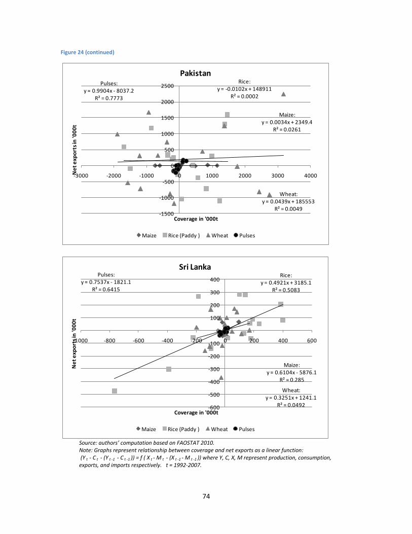
74

Figure 24 (continued)

Source: authors’ computation based on FAOSTAT 2010. Note: Graphs represent relationship between coverage and net exports as a linear function: (Y t - C t - (Y t -1 - C t -1 )) = f ( X t - M t - (X t -1 - M t -1 )) where Y, C, X, M represent production, consumption, exports, and imports respectively. t = 1992-2007.

Maize:y = 0.0034x + 2349.4

R² = 0.0261

Rice:y = -0.0102x + 148911

R² = 0.0002

Wheat:y = 0.0439x + 185553

R² = 0.0049

Pulses:y = 0.9904x - 8037.2

R² = 0.7773

-1500

-1000

-500

0

500

1000

1500

2000

2500

-3000 -2000 -1000 0 1000 2000 3000 4000Ne

t e

xpo

rts

in '0

00

t

Coverage in '000t

Pakistan

Maize Rice (Paddy ) Wheat Pulses

Maize:y = 0.6104x - 5876.1

R² = 0.285

Rice:y = 0.4921x + 3185.1

R² = 0.5083

Wheat:y = 0.3251x + 1241.1

R² = 0.0492

Pulses:y = 0.7537x - 1821.1

R² = 0.6415

-600

-500

-400

-300

-200

-100

0

100

200

300

400

-1000 -800 -600 -400 -200 0 200 400 600

Ne

t e

xpo

rts

in '0

00

t

Coverage in '000t

Sri Lanka

Maize Rice (Paddy ) Wheat Pulses

75

4 Climate change scenarios

Introducing the effects of different climate change scenarios into the overall food and

agriculture scenarios presents a particular challenge – in particular, how to take into account the

range of plausible pathways for greenhouse gas (GHG) emissions. The available global

circulation models (GCMs) translate those emission scenarios into varying temperature and

precipitation outcomes. While the general consequences of increasing atmospheric

concentrations of GHGs are increasingly well known, great uncertainty remains about how

climate change effects will play out in specific locations. Therefore this paper relies on 12

alternative climate change scenarios that will help provide the range of potential outcomes from

climate change for South Asia. These 12 SRES9 scenarios are the result of the combination of

GHG paths and alternative GCM models.

Figure 25 shows the range of average surface temperature outcomes for the GHG pathways in

the SRES scenarios of the IPCC. By 2050, global surface warming projections in the A1B, A2, and

B1 scenarios are approximately identical, at about 1°C above the reference period of the late

20th century. Temperature increases diverge significantly after 2050 however, with the A2

scenario resulting in the highest increase (about 3.5 °C) by the end of the 20th century. Because

the analysis in this paper stops in 2050, it does not capture the effects of the large increases

expected in the second half of the 21st century.

9 Special Report on Emissions Scenarios (SRES) of the Intergovernmental Panel on Climate Change (IPCC).

76

Figure 25 Emissions scenarios: change in temperature

Table 7 displays the consequences of different emission paths (GHG pathways) in terms of

precipitation and temperature. First, as average temperatures rise, so does annual

precipitation. A 1°C increase in average temperature typically results in less than a 1 percent

increase in average annual precipitation. Temperature increases of over 2°C result in 2–5

percent increases in precipitation. Second, with identical GHG emissions, the different GCM

differ substantially in their climate change predictions. The most extreme comparison is with

the outcomes of the B1 scenario. The CSIRO GCM has almost no increase in average annual

precipitation and the smallest temperature increase of any of the GCM/GHG scenario

combinations. The MIROC GCM has the second largest increase in precipitation (within the B1

scenario) and one of the largest increases in average temperature. So, it appears that the CSIRO

scenarios are relatively dryer and cooler while the MIROC results describe a warmer and more

humid future. The ECH and CNR models display intermediate pictures where the ECH GCM

appears to forecast a less wet future than the CNR models.10

10 See www.ipcc.ch/publications_and_data/ar4/wg1/en/suppl/chapter10/Ch10_indiv-maps.html for

detailed results and maps.

77

Table 7 Alternative GCM model results in terms of changes in temperature and precipitation

Source: From Nelson et al., 2010. Note: For an exhaustive discussion on the GCMs, see appendix II of Nelson et al., 2010. Model acronyms are explained in Chapter 2.

In the following sections, each scenario will be named by the three first letters of the GCM

followed by the two first letter of the SRES scenario (e.g. mir_a1 will stand for MIROC GCM,

SRES A1B).

4.1 Yield impact of Climate Change

This section discusses the impact of the different climate change scenarios on the yields of

maize, wheat, rice, soybeans and groundnuts as estimated by the DSSAT model.

4.1.1 Impact of climate change on global yields

The DSSAT simulations in Figure 26 show the change in yields driven by climate change for

different scenarios at the global level. Simple averages across scenarios are also displayed.

First, all scenarios show a decline in average yields (weighted by initial production) from -0.6

percent (csi_b1 scenario) to -11 percent (mir_a1 scenario). These extreme values match the

78

extreme temperature and precipitation scenarios discussed in Table 7 – with the wetter and

warmer scenario (mir_a1) having the most adverse effects.

The most affected crops are wheat and maize – and both show a yield decline of 5 percent or

more based on a simple average across scenarios. Heterogeneity among scenarios at the world

level is high – as expressed in coefficients of variation across scenarios of 45 percent and 75

percent for wheat and maize, respectively. Rice (rainfed) and soybeans are less affected on

average but the variance across scenarios are also higher (160 percent for rice).The extremes

(yield declines of 10 percent or more) are found for groundnut and wheat respectively in

scenarios cnr_a1 and cnr_a2I; and for maize and soybeans in scenarios mir_a1 and mir_a2,

respectively.

Second, a broad hierarchy can be defined across scenarios from the most adverse to the more

moderate: mir_a1, mir_a2, cnr_a1, mir_b1, cnr_a2, cnr_b1, ech_a1, csi_a1, ech_b1, ech_a2,

csi_a2, csi_b1. Of course, some crops display some special behavior: for example, groundnut

production is less affected by the mir scenarios than by other scenarios, even though the former

are on average more adverse.

Figure 26 Changes in world yields (rainfed) due to climate change for different scenarios and selected crops. Weighted by initial area and production.

-15.0%

-10.0%

-5.0%

0.0%

5.0%

10.0%

15.0%

20.0%

25.0%

30.0%

GroundNut Area weighted Maize Area weighted

Rice Area weighted Soybean Area weighted

Wheat Area weighted Selected crops Area weighted

79

Source: DSSAT model simulations. Note: Upper graph is weighed by area, lower graph is weighed by production.

A comparison of the lower and upper panels of Figure 26 shows that the average changes in

yields weighted by initial production are more pessimistic than the average changes weighted by

area (e.g. in scenario cnr_a1 the increase in average soybean yield is 6.7 percent whereas yield

is projected to decreases by 18 percent when weighted by production). This pattern is found for

all crops and all scenarios. The explanation is simple: the regions with the highest yield are

going to be relatively more affected by climate change than initially low productivity regions.

This may involve significant changes in trade patterns to the extent that high yield regions are

the source of traditional exports.

-30.0%

-25.0%

-20.0%

-15.0%

-10.0%

-5.0%

0.0%

5.0%

10.0%

GroundNut Production weighted Maize Production weighted

Rice Production weighted Soybean Production weighted

Wheat Production weighted Selected crops Production weighted

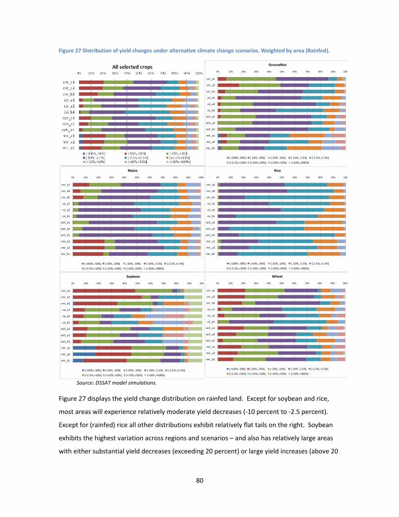
80

Figure 27 Distribution of yield changes under alternative climate change scenarios. Weighted by area (Rainfed).

Source: DSSAT model simulations.

Figure 27 displays the yield change distribution on rainfed land. Except for soybean and rice,

most areas will experience relatively moderate yield decreases (-10 percent to -2.5 percent).

Except for (rainfed) rice all other distributions exhibit relatively flat tails on the right. Soybean

exhibits the highest variation across regions and scenarios – and also has relatively large areas

with either substantial yield decreases (exceeding 20 percent) or large yield increases (above 20

0% 10% 20% 30% 40% 50% 60% 70% 80% 90% 100%

cnr_a1

cnr_a2

cnr_b1

csi_a1

csi_a2

csi_b1

ech_a1

ech_a2

ech_b1

mir_a1

mir_a2

mir_b1

GroundNut

]-100%,-50%[ [-50%,-20%[ [-20%,-10%[ [-10%,-2.5%[ [-2.5%,+2.5%[

[+2.5%,+10%[ [+10%,+20%[ [+20%,+50%[ [+50%,+400%[

0% 10% 20% 30% 40% 50% 60% 70% 80% 90% 100%

cnr_a1

cnr_a2

cnr_b1

csi_a1

csi_a2

csi_b1

ech_a1

ech_a2

ech_b1

mir_a1

mir_a2

mir_b1

Maize

]-100%,-50%[ [-50%,-20%[ [-20%,-10%[ [-10%,-2.5%[ [-2.5%,+2.5%[

[+2.5%,+10%[ [+10%,+20%[ [+20%,+50%[ [+50%,+400%[

0% 10% 20% 30% 40% 50% 60% 70% 80% 90% 100%

cnr_a1

cnr_a2

cnr_b1

csi_a1

csi_a2

csi_b1

ech_a1

ech_a2

ech_b1

mir_a1

mir_a2

mir_b1

Rice

]-100%,-50%[ [-50%,-20%[ [-20%,-10%[ [-10%,-2.5%[ [-2.5%,+2.5%[

[+2.5%,+10%[ [+10%,+20%[ [+20%,+50%[ [+50%,+400%[

0% 10% 20% 30% 40% 50% 60% 70% 80% 90% 100%

cnr_a1

cnr_a2

cnr_b1

csi_a1

csi_a2

csi_b1

ech_a1

ech_a2

ech_b1

mir_a1

mir_a2

mir_b1

Soybean

]-100%,-50%[ [-50%,-20%[ [-20%,-10%[ [-10%,-2.5%[ [-2.5%,+2.5%[

[+2.5%,+10%[ [+10%,+20%[ [+20%,+50%[ [+50%,+400%[

0% 10% 20% 30% 40% 50% 60% 70% 80% 90% 100%

cnr_a1

cnr_a2

cnr_b1

csi_a1

csi_a2

csi_b1

ech_a1

ech_a2

ech_b1

mir_a1

mir_a2

mir_b1

Wheat

]-100%,-50%[ [-50%,-20%[ [-20%,-10%[ [-10%,-2.5%[ [-2.5%,+2.5%[

[+2.5%,+10%[ [+10%,+20%[ [+20%,+50%[ [+50%,+400%[

81

percent). In several scenarios (cnr and mir types), maize and wheat have large areas where a

yield decrease of more than 20 percent is predicted.

The previous discussion was focused on rainfed agriculture which, at least for the crops

considered in this paper, represents more than 80 percent of cultivated area (see Figure 28). In

the DSSAT simulations, irrigated crops are only affected by changes in temperature – in other

words water availability is considered to be sufficient to maintain optimal level. However,

changes in yields are more important for irrigated than rainfed agriculture (between -6 percent

and -11 percent for the production weighted average for selected crops across all scenarios).

Compared to rainfed cultivation, yield decreases in irrigated agriculture are larger but less

variable across scenarios (standard deviation about 20 percent for most crops). Indeed, only

temperature variability across scenarios plays a role here. Among irrigated crops, changes in

temperature affect wheat yields most, with yield decreases of between 10 percent and 16

percent at the world level (versus less than 10 percent for rainfed wheat). As noted earlier, this

implies that the impact of climate change will be larger in regions with initially better yields

(driven by better conditions under rainfed management or by irrigation).11

Figure 28 Share of rainfed agriculture at the world level for selected crops

Source: IMPACT model database

The specific case of rice warrants separate discussion. As shown in Figure 26 and Figure 27,

rainfed rice is relatively little affected by climate change (yield changes of between +1 percent

and -3 percent). Figure 29 displays the average change in yields for rainfed and irrigated rice,

11 This also implies that in some regions the adverse effects of higher temperatures are compensated by

additional water for rainfed crops.

0% 20% 40% 60% 80% 100%

GroundNut

Maize

Rice

Soybean

Wheat

Irrigated Rainfed

82

showing that the effects on irrigated rice will be substantially larger (two to three times) than

for rainfed case. Therefore, the optimistic picture for rainfed rice changes when considering

overall rice production since most rice comes from irrigated land. More precisely, rice yields will

decrease by 6.6 percent on average when calculated over all scenarios (with production as

weights).

Figure 29 Distribution of change in global yield of rice (weighted by production) for rainfed and irrigated cultivation.

Source: IMPACT model database and DSSAT simulations.

4.1.2 Impact on yields in South Asia

While the previous section discussed the impact of different climate change scenarios on yields

on a global level, this section provides further details for the SAFTA region and the four SAFTA

countries that are explicitly represented in the model.

Figure 30 depicts changes in yields in South Asia for selected crops (rainfed) under different

climate change scenarios. Considering simple averages across crops and scenarios reveals that

contrary to earlier findings on the global level, the results weighted by area are slightly more

pessimistic (-3.5 percent decrease in yields on average) than those weighted by production (-2.8

percent decrease in yields on average). Across scenarios, scenarios cnr_a1 and cnr_a2 have

prominent negative effects on average yields (-8.6 percent and -9.1 percent area weighted

decline in yields, respectively) while scenarios mir_a1 and mir_a2 lead to slight increases in

average yields. The results weighted by area are relatively close to those weighted by

production, indicative of relatively similar productivity across SAFTA counties for the crops

under consideration. These results differ from those on the global level where heterogeneity in

-4.0%

-3.0%

-2.0%

-1.0%

0.0%

1.0%

-12.0% -10.0% -8.0% -6.0% -4.0% -2.0% 0.0%

Ra

infe

d

Irrigated

83

productivity across countries led to a more pronounced gap between the production and area

weighted results.

Average yield changes across different scenarios are negative for all crops irrespective of the

type of weights used (i.e. production or area). Wheat and soybeans are the most severely

impacted crops as their yields (weighted by area) are expected to decline by -11.5 percent and -

8.2 percent, respectively. On the other hand, groundnuts and rice are the least affected crops.

Nevertheless, a closer look at average yield change for groundnuts for different scenarios shows

very high coefficients of variation (779 percent using area weights and 352 percent using

production weights). More specifically, scenarios cnr_a1, cnr_a2 and cnr_b1 result in significant

decreases in groundnut yields, while mir_a1, mir_a2 and mir_b1 lead to significant yield

increases. With respect to wheat, all climate change scenarios lead to a decline in yields in

SAFTA countries, and are more pronounced in the ech_a1 and csi_a2 scenarios (-19.4 percent

and -14.2 percent using area weights, respectively).

84

Figure 30 Changes in crop yields in South Asia (rainfed) due to climate change for different scenarios and selected crops. Weighted by initial area and production.

Source: DSSAT model simulations.

The overall distribution of yield changes on rainfed land in SAFTA countries is presented Figure

31 - and turns out to be quite similar to the corresponding distribution on the global level. A

moderate (-10 percent to -2.5 percent) decrease in yields affects large areas across all scenarios.

Notable exceptions to this case are wheat and soybeans which exhibit a more pronounced

negative yield change (-20 percent to -10 percent). With respect to groundnuts there are large

areas with large yield increases (20 percent to 50 percent), while in the case of wheat more than

half of rainfed areas are impacted by significant yield decreases ranging from -50 percent to -10

percent.

-30.0%

-25.0%

-20.0%

-15.0%

-10.0%

-5.0%

0.0%

5.0%

10.0%

15.0%

20.0%

cnr_a1 cnr_a2 cnr_b1 csi_a1 csi_a2 csi_b1 ech_a1 ech_a2 ech_b1 mir_a1 mir_a2 mir_b1 SimpleAverage

GroundNut Area weighted Maize Area weighted Rice Area weighted

Soybean Area weighted Wheat Area weighted Selected crops Area weighted

85

Figure 31 Distribution of yield changes under alternative climate change scenarios. Weighted by area (Rainfed).

Source: DSSAT model simulations.

Figure 32 further decomposes yield changes in Bangladesh, India, Pakistan and Sri Lanka.

Considering average yield changes across all crops and scenarios, all four countries suffer from

decreasing yields, with Pakistan and India being affected most (suffering average yield decreases

of respectively 9.6 percent and -3.9 percent when weighted by production). In the case of

0% 10% 20% 30% 40% 50% 60% 70% 80% 90% 100%

cnr_a1

cnr_a2

cnr_b1

csi_a1

csi_a2

csi_b1

ech_a1

ech_a2

ech_b1

mir_a1

mir_a2

mir_b1

All Selected Crops

]-100%,-50%[ [-50%,-20%[ [-20%,-10%[ [-10%,-2.5%[ [-2.5%,+2.5%[

[+2.5%,+10%[ [+10%,+20%[ [+20%,+50%[ [+50%,+400%[

0% 10% 20% 30% 40% 50% 60% 70% 80% 90% 100%

cnr_a1

cnr_a2

cnr_b1

csi_a1

csi_a2

csi_b1

ech_a1

ech_a2

ech_b1

mir_a1

mir_a2

mir_b1

GroundNut

]-100%,-50%[ [-50%,-20%[ [-20%,-10%[ [-10%,-2.5%[

[-2.5%,+2.5%[ [+2.5%,+10%[ [+10%,+20%[ [+20%,+50%[

0% 10% 20% 30% 40% 50% 60% 70% 80% 90% 100%

cnr_a1

cnr_a2

cnr_b1

csi_a1

csi_a2

csi_b1

ech_a1

ech_a2

ech_b1

mir_a1

mir_a2

mir_b1

Maize

[-50%,-20%[ [-20%,-10%[ [-10%,-2.5%[ [-2.5%,+2.5%[

[+2.5%,+10%[ [+10%,+20%[ [+20%,+50%[ [+50%,+400%[

0% 10% 20% 30% 40% 50% 60% 70% 80% 90% 100%

cnr_a1

cnr_a2

cnr_b1

csi_a1

csi_a2

csi_b1

ech_a1

ech_a2

ech_b1

mir_a1

mir_a2

mir_b1

Rice

]-100%,-50%[ [-50%,-20%[ [-20%,-10%[ [-10%,-2.5%[

[-2.5%,+2.5%[ [+2.5%,+10%[ [+10%,+20%[ [+20%,+50%[

0% 10% 20% 30% 40% 50% 60% 70% 80% 90% 100%

cnr_a1

cnr_a2

cnr_b1

csi_a1

csi_a2

csi_b1

ech_a1

ech_a2

ech_b1

mir_a1

mir_a2

mir_b1

Soybean

[-50%,-20%[ [-20%,-10%[ [-10%,-2.5%[ [-2.5%,+2.5%[

[+2.5%,+10%[ [+10%,+20%[ [+20%,+50%[

0% 10% 20% 30% 40% 50% 60% 70% 80% 90% 100%

cnr_a1

cnr_a2

cnr_b1

csi_a1

csi_a2

csi_b1

ech_a1

ech_a2

ech_b1

mir_a1

mir_a2

mir_b1

Wheat

[-50%,-20%[ [-20%,-10%[ [-10%,-2.5%[ [-2.5%,+2.5%[

[+2.5%,+10%[ [+10%,+20%[ [+20%,+50%[ [+50%,+400%[

86

Pakistan there are particularly large decreases in average yields for scenarios ech_a1 (-25.1

percent) and ech_b1 (-16.3 percent).

The 9.6 percent decrease in average crop yield in Pakistan is mainly driven by significant drops in

rice productivity (-35.1 percent) and groundnut yield (-49 percent) – for these crops all scenarios

exhibiting yield decreases. Other crops in Pakistan including maize and wheat are less affected,

suffering average yield decreases of respectively -3.4 percent and -12.1 percent. In some

scenarios (cnr_a1, cnr_a2 and cnr_b1) maize yields in Pakistan even increase.

Average groundnuts yields decrease most significantly in Bangladesh (-12.8 percent). On the

other hand, groundnut productivity in India increases by 8.6 percent under scenario mir_a1. On

average across scenarios, rice yields in SAFTA suffer only moderately (except the case of

Pakistan discussed previously). Wheat yields decrease across all countries and scenarios, most

significantly so in scenario ech_a1. Finally, average soybean yields in Sri Lanka increase (by 9.2

percent).

87

Figure 32 Distribution of yield changes across countries under alternative climate change scenarios. Weighted by production (rainfed).

Source: DSSAT model simulations

The results discussed above concern only the impact of climate change scenarios on yields of

selected crops under rainfed conditions. However, the share of irrigated crops is significant in

SAFTA countries (see Figure 33). For example, Pakistan is one of the leading countries in the

world as far as irrigated agriculture is concerned. Irrigated land accounts for about 80 percent

of total cropland in that country - and about 90 percent of wheat and 100 percent of the rice

-30.0%

-25.0%

-20.0%

-15.0%

-10.0%

-5.0%

0.0%

5.0%

10.0%

cnr_a1 cnr_a2 cnr_b1 csi_a1 csi_a2 csi_b1 ech_a1 ech_a2 ech_b1 mir_a1 SimpleAverage

All Crops

Bangladesh India Pakistan Sri Lanka

-70.0%

-60.0%

-50.0%

-40.0%

-30.0%

-20.0%

-10.0%

0.0%

10.0%

20.0%

cnr_a1 cnr_a2 cnr_b1 csi_a1 csi_a2 csi_b1 ech_a1 ech_a2 ech_b1 mir_a1 SimpleAverage

GroundNut

Bangladesh India Pakistan Sri Lanka

-20.0%

-15.0%

-10.0%

-5.0%

0.0%

5.0%

10.0%

15.0%

20.0%

cnr_a1 cnr_a2 cnr_b1 csi_a1 csi_a2 csi_b1 ech_a1 ech_a2 ech_b1 mir_a1 SimpleAverage

Maize

Bangladesh India Pakistan Sri Lanka

-60.0%

-50.0%

-40.0%

-30.0%

-20.0%

-10.0%

0.0%

10.0%

20.0%

cnr_a1 cnr_a2 cnr_b1 csi_a1 csi_a2 csi_b1 ech_a1 ech_a2 ech_b1 mir_a1 SimpleAverage

Rice

Bangladesh India Pakistan Sri Lanka

-30.0%

-20.0%

-10.0%

0.0%

10.0%

20.0%

30.0%

40.0%

cnr_a1 cnr_a2 cnr_b1 csi_a1 csi_a2 csi_b1 ech_a1 ech_a2 ech_b1 mir_a1 SimpleAverage

Soybean

Bangladesh India Pakistan Sri Lanka

-35.0%

-30.0%

-25.0%

-20.0%

-15.0%

-10.0%

-5.0%

0.0%

cnr_a1 cnr_a2 cnr_b1 csi_a1 csi_a2 csi_b1 ech_a1 ech_a2 ech_b1 mir_a1 SimpleAverage

Wheat

Bangladesh India Pakistan Sri Lanka

88

and soybean crops receive irrigation. Furthermore, irrigation plays an important role in Indian

agriculture as well - 80 percent of wheat and 50 percent of rice is cultivated under irrigated

conditions. On the other hand, in Sri Lanka irrigated land is mostly used for rice with maize and

groundnuts completely rainfed.

Figure 33 Share of rainfed agriculture at the world level for selected crops

Source: IMPACT model database

Given the importance of irrigation in Pakistan, Figure 34 compares yield distributions for

selected crops under rainfed and irrigated conditions. Since in the case of irrigated crops

climate change does not change water availability (i.e. water is assumed to be sufficient and

maintained at an optimal level), the only driver of yield change in irrigated crops is changes in

temperature (as opposed to rainfed crops where both temperature and precipitation changes

are also considered). For groundnuts the results show similar patterns across all scenarios:

averega irrigated yield decreases (-25.3 percent) are smaller than average rainfed yield

decreases (-48.4 percent). The results are more variable in the cases of rice and wheat: in some

scenarios rainfed yields decrease more than irrigated yields while in other scenarios the

0% 20% 40% 60% 80% 100%

BAN

IND

PAK

SRL

BAN

IND

PAK

SRL

BAN

IND

PAK

SRL

BAN

IND

PAK

SRL

BAN

IND

PAK

SRL

Gro

un

dN

ut

Mai

zeR

ice

So

ybe

anW

he

at

Irrigated Rainfed

89

opposite holds. In the relatively cooler and drier climate change scenarios rainfed rice yields

decrease more than yields of irrigated rice, while in the relatively more humid and warm

scenarios irrigated wheat yields suffer more than rainfed wheat yields. In the case of maize

irrigated yields decline more than rainfed yields. In scenarios cnr_a1, cnr_a2 and cnr_b1 climate

change leads to an increase in yields of rainfed maize and a decrease in irrigated maize yields.

Figure 34 Distribution of yield of selected crops in Pakistan for rainfed and irrigated production (weighted by production)

Source: DSSAT model simulations.

-60%

-50%

-40%

-30%

-20%

-10%

0%

10%

20%

30%

-60% -50% -40% -30% -20% -10% 0%R

a

i

n

f

e

d

Irrigated

GroundNut

Maize

Rice

Wheat

90

5 Trade Policy Scenarios and Simulations Results

This Chapter presents the different trade policy scenarios considered and discusses the

simulation results. Due to the relatively high number of scenarios (124)12, it is not practical to

display detailed results for all simulations.13 Moreover, the goal in this paper is not to determine

what will be the detailed consequences of each potential climate scenario but rather to assess

how changes in trade policy might allow South Asia to mitigate the effects of an uncertain

future. For this reason, simple averages and their variation across climate scenarios are

displayed for each trade policy baseline in order to identify a potentially optimal policy. Indeed,

there is no a-priori bias with respect to the occurrence of one scenario or another. In addition,

the analysis places special emphasis on presenting the results by individual South Asian

countries, given that a single SAFTA aggregate would be dominated by India and give insufficient

attention to the other SAFTA countries.

The next section looks at the trade policy alternatives that constitute the different baselines,

followed by a discussion of simulation results in section 5.2. All simulation results will be

compared against the perfect mitigation case: the latter figures as the equivalent of a 13th SRES

scenario in which yields are not affected by climate change.

5.1 Trade policy alternatives as different baselines for climate change

scenarios As discussed earlier in Chapter 2, assumptions regarding trade policies14 are critical at different

levels. Since policy makers exert control over trade policy, this paper considers eight different

trade policy scenarios for possible implementation between 2010 and 2024 and which shape the

landscape in which climate change will occur. The potential role of trade policies (mainly tariffs

in this paper) in further shaping the effects of climate change can be summarized as follows:

Under the assumption that they are not endogenous to world prices, ad-valorem duties

amplify domestic price increases caused by climate change. Therefore, duties magnify

12 The 124 scenarios were derived as follows: (12 SRESxCGM scenarios + 1 perfect mitigation scenario) x 8

trade policy baselines. 13

All the results for each scenario are available from the authors upon request. 14

Other assumptions regarding the baseline are discussed in section ‎2.2.2.

91

the cost burden for consumers by applying an additional tax on the exogenous price

change. This is a direct effect.

Duties affect relative prices between sectors of an economy which in turn affects the

relative size distribution between sectors. Therefore, the size of the agricultural sector

(which is the sector that is directly affected by climate change) compared to the size of

other sectors (manufacturing and services) is to an important extent influenced by the

type of trade policy:

a. Since protection rates are higher for the agricultural sector compared to the

other sectors in all SAFTA countries, unilateral trade liberalization would lead to

a reallocation of production factors from agriculture to other sectors, thus

reducing the size of the agricultural sector. Since the impact of climate change

(i.e. changes in agricultural productivity) on overall GDP is lower for economies

whose GDP is less dependent on agriculture, unilateral trade liberalization may

facilitate compensating those in the agricultural sector who stand to lose from

climate change.

b. In case of multilateral trade liberalization, comparative advantages will play out

to their maximum. New market opportunities may arise for some sectors -

including the agricultural sector (e.g. for rice exports to Japan). The impact of

multilateral trade liberalization on the consequences of climate change (i.e. on

agricultural production and incomes) would depend on how climate change

affects the productivity of agricultural commodities in which South Asian

countries have a comparative advantage.

c. If some agricultural sub-sectors (commodities) are excluded from trade

liberalization, it will be important for the region to assess the extent to which

these sub-sectors are affected by climate change (relative to other less

protected sub-sectors). If the sub-sectors that continue to be protected are

also those which are affected most by climate change, then protectionist

policies will maintain artificial specialization (in contrast to comparative

advantage resulting from free trade) in activities that will face severe

productivity losses.

Trade liberalization changes the extent to which countries depend on world markets,

their degree of openness, and how they are exposed to different price shocks in world

92

markets through the terms of trade effect. Depending on the exposure to world prices

and the structure of trade, the cost to the domestic economy of a relative price shock

will vary. Relative prices exert their influence through two channels: i.e. relative prices

between domestic and foreign producers within a given sector, and relative prices

between exports and imports, across sectors. If trade liberalization leads to higher

imports of a commodity that increases in price as a result of climate change, the cost

for the importing economy will increase as well.

Discriminatory trade policies (e.g. preferential trade agreements) can play an important

role by shifting regional trade patterns into a particular direction. Assuming that policy

makers can correctly predict which countries will be more negatively affected by

climate change, it will be important that they get market access for their own exports

to these markets and that they develop trade relations with other regions to satisfy

their own demand. In other words, it may be optimal to use trade policy to diversify

trading partners in order to reinforce trade relations with regions for which climate

shocks will be negatively correlated with the domestic economy, as in a portfolio

management strategy. This can act as an incentive to pursue a non regional integration

strategy if the region does not provide enough diversification opportunities.

The previous explanations have made it clear that there is a need to analyze alternative trade

policy scenarios combining different mixes of sectoral and geographical trade liberalization.

5.1.1 Description of trade policy alternatives

A total of eight trade policy alternatives were considered, each involving a different mix of

potential tariff reductions compared to their starting levels in 2007 (see Table 8):

1. Baseline tariffs (BASE): In this alternative, tariffs are frozen at their 2007 levels.

2. SAFTA implementation (SAFTA): This alternative describes the full implementation of

SAFTA including sensitive products (see the SAFTA scenario description in Bouet and

Corong 2009).

3. SAFTA-plus alternative (SAFTAFULL): This alternative involves the full elimination of all

tariffs between South Asian countries.

4. Unilateral liberalization (UNISEN): SAFTA countries unilaterally liberalize trade in all

sectors (agriculture and non-agriculture) except for sensitive products. For each SAFTA

93

economy the list of sensitive products is identical to the one used in the SAFTA

agreement. This alternative involves keeping tariffs on most key agricultural imports.

5. Unilateral elimination of all tariffs in agriculture (UNIAGR): This alternative leads to a

sharp decline in agricultural prices relative to manufacturing prices and a reallocation of

resources towards the latter sector.

6. Full liberalization of SAFTA economies towards all partners for all sectors (UNIALL): This

alternative involves a complete unilateral liberalization of SAFTA economies. The

liberalization of the manufacturing sector dampens the shock on relative prices

compared to the UNIAGR alternative.

7. Free trade among all countries in Asia and Oceania (FTA): This alternative involves

strong regional integration alternative by abolishing any remaining tariff restrictions

between the South Asian countries and Central Asia, China, developed East Asian

economies, ASEAN countries, and Australia and New Zealand (ANZCERTA). For South

Asia this alternative creates both new market opportunities (e.g. in the initially highly

protected South Korea and Japanese markets) and increased competition in domestic

markets from other participating countries.

8. Complete trade liberalization (MULTI): This alternative involves tariff elimination at the

global level. This very ambitious alternative provides a benchmark for all other (less

ambitious) alternatives.

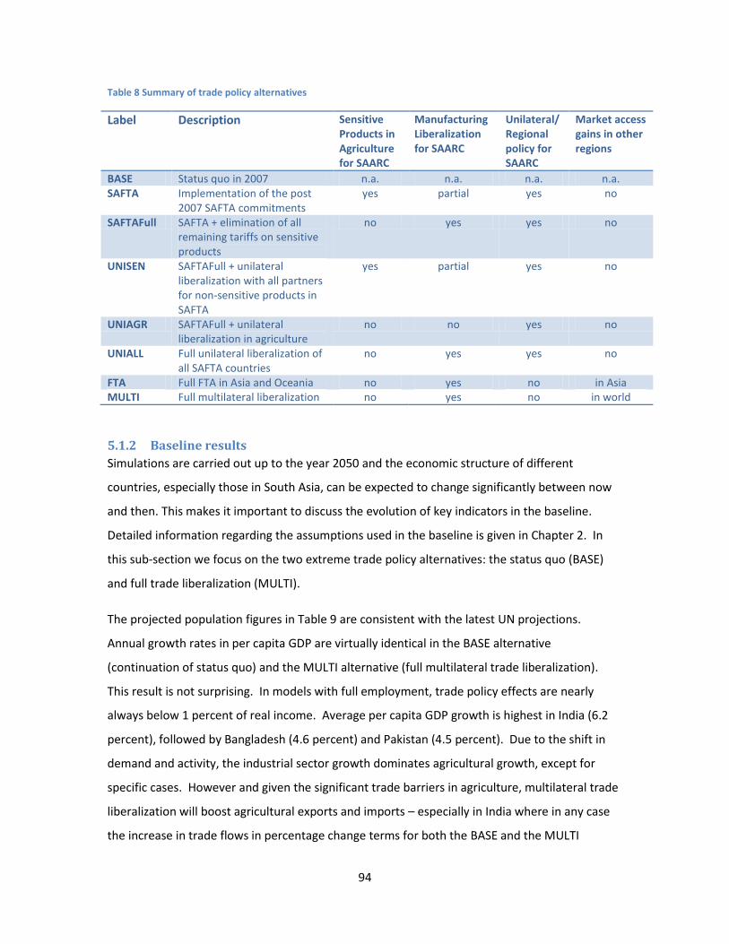
94

Table 8 Summary of trade policy alternatives

Label Description Sensitive Products in Agriculture for SAARC

Manufacturing Liberalization for SAARC

Unilateral/ Regional policy for SAARC

Market access gains in other regions

BASE Status quo in 2007 n.a. n.a. n.a. n.a. SAFTA Implementation of the post

2007 SAFTA commitments yes partial yes no

SAFTAFull SAFTA + elimination of all remaining tariffs on sensitive products

no yes yes no

UNISEN SAFTAFull + unilateral liberalization with all partners for non-sensitive products in SAFTA

yes partial yes no

UNIAGR SAFTAFull + unilateral liberalization in agriculture

no no yes no

UNIALL Full unilateral liberalization of all SAFTA countries

no yes yes no

FTA Full FTA in Asia and Oceania no yes no in Asia MULTI Full multilateral liberalization no yes no in world

5.1.2 Baseline results

Simulations are carried out up to the year 2050 and the economic structure of different

countries, especially those in South Asia, can be expected to change significantly between now

and then. This makes it important to discuss the evolution of key indicators in the baseline.

Detailed information regarding the assumptions used in the baseline is given in Chapter ‎2. In

this sub-section we focus on the two extreme trade policy alternatives: the status quo (BASE)

and full trade liberalization (MULTI).

The projected population figures in Table 9 are consistent with the latest UN projections.

Annual growth rates in per capita GDP are virtually identical in the BASE alternative

(continuation of status quo) and the MULTI alternative (full multilateral trade liberalization).

This result is not surprising. In models with full employment, trade policy effects are nearly

always below 1 percent of real income. Average per capita GDP growth is highest in India (6.2

percent), followed by Bangladesh (4.6 percent) and Pakistan (4.5 percent). Due to the shift in

demand and activity, the industrial sector growth dominates agricultural growth, except for

specific cases. However and given the significant trade barriers in agriculture, multilateral trade

liberalization will boost agricultural exports and imports – especially in India where in any case

the increase in trade flows in percentage change terms for both the BASE and the MULTI

95

alternatives is highest. A notable exception is formed by exports of staples where the

percentage growth in India’s trade flows is exceeded by those in Bangladesh, Pakistan and Sri

Lanka. Not surprisingly, trade growth under full multilateral trade liberalization is systematically

higher than that in the base trade policy scenario for all South Asian countries.

Table 9 Baseline trade policy alternative: evolution of selected indicators

Bangladesh India Pakistan Sri Lanka Rest of South Asia

World

Population in 2050 (Mil. inhabitants) 222 1,611 332 22 123 9,058

An

nu

al g

row

th r

ate

(Bas

e t

rad

e p

olic

y)

GDP per Capita 4.6% 6.2% 4.5% 4.1% 3.8% 3.9%

Imports (staple) 4.4% 9.8% 7.2% 4.5% 6.6% 5.4%

Imports (agrifood) 5.0% 7.0% 4.8% 3.0% 5.7% 4.5%

Imports (industrial) 5.9% 10.3% 8.4% 5.3% 7.0% 5.1%

Exports (staple) 7.9% 7.0% 7.4% 7.7% 7.0% 5.4%

Exports (agrifood) 5.3% 10.5% 9.9% 4.7% 3.7% 4.5%

Exports (industrial) 5.0% 11.1% 8.7% 6.1% 9.1% 5.1%

An

nu

al g

row

th r

ate

(Mu

ltila

tera

l fu

ll

libe

raliz

atio

n )

GDP per Capita 4.6% 6.2% 4.5% 4.1% 3.8% 3.9%

Imports (staple) 4.6% 11.6% 7.7% 5.5% 7.4% 5.9%

Imports (agrifood) 5.5% 8.4% 6.1% 3.9% 6.1% 5.4%

Imports (industrial) 6.6% 10.8% 8.9% 5.5% 7.5% 5.3%

Exports (staple) 9.4% 7.8% 8.1% 9.1% 9.0% 5.9%

Exports (agrifood) 6.0% 12.6% 10.4% 5.2% 4.2% 5.4%

Exports (industrial) 5.7% 11.5% 9.3% 6.5% 9.7% 5.3%

Source: Simulations with MIRAGE.

5.2 Simulation Results

5.2.1 Impact of climate change and trade policy on real income

Figure 35 displays the evolution of changes in real income by 2050 for the world across trade

policy alternatives and climate change scenarios. The impact of climate change on world GDP is

relatively small which is not unexpected given the steady decline in the share of agriculture in

GDP. However, even the small relative change in world GDP still represents between -$740

billion and +$1,015 billion (in 2004 constant USD). More interesting is the fact that there are

relatively large variations across climate change scenarios - with the largest increase seen in

scenario csi_b1 and the largest decrease obtained in scenario cnr_a (see Table 7 on page 76 for

climate change scenario definitions). Furthermore, trade policy options have only limited

effects on real world income. Full multilateral trade liberalization (the MULTI trade policy

alternative) leads to an increase in real income compared to the status quo (the BASE trade

96

policy alternative) only in 5 out of the 12 climate change scenarios – a testimony to the

complexity of the mechanisms at play. Nevertheless, trade liberalization does play a more

important role in certain specific cases: for example, full multilateral trade liberalization has

minimal effects on real income in the csi climate change scenarios but maximizes income gains

in the mir climate scenarios while limiting losses significantly in the ech_a1 scenario. The csi

climate scenarios, which will be discussed in greater detail in subsection 5.2.5 below, are the

most sensitive to trade policy. The full multilateral liberalization trade policy alternative (MULTI)

results in a relatively large expansion of trade in the baseline leads to more limited readjustment

and therefore, less important real income gains from trade.

Figure 35 Annual changes in world real income by 2050 - by climate change scenario and trade policy alternative

Source: Simulations with MIRAGE

SAFTA is one of the regions that are most negatively affected by climate change in terms of

income (see Figure 36), especially Pakistan (up to 4 percent income loss) followed by Bangladesh

and Sri Lanka. On the other hand, India benefits from a slight increase in real income and acts as

a stabilizer in the region. A decomposition by trade policy scenario across climate change

scenarios (Figure 37) illustrates that there is relatively high dispersion among countries with

respect to the impact of trade policy on real income. There is a clear negative correlation

between country size and the degree of dispersion, i.e. the impact of different trade

liberalization alternatives varies more significantly in the case of Sri Lanka than in that of India.

97

In addition, Sri Lanka and the Rest of South Asia experience bigger proportional declines in real

income as the degree of liberalization increases. Detailed results for each climate change

scenario and trade liberalization policy are presented in Table 19 in the Appendix.

Figure 36 Changes in real incomes in SAFTA countries compared to other regions and countries (simple averages across climate change scenarios)

Source: Simulations with MIRAGE.

98

Figure 37 Real Income effects (simple averages and extreme values) of climate change in SAFTA countries – by trade policy alternative

(continued on next page)

99

Note: Length of bars represent minima and maxima across climate scenarios. Source: Simulations with MIRAGE.

Table 10 is an attempt at summarizing the ranking (based on the real income criteria) of

different trade policy alternatives for SAFTA countries. Optimistic describes the highest real

income increase across climate scenarios, average the average change and pessimistic the most

adverse real income change. The results show that all countries except India would favor more

conservative trade liberalization scenarios. For India, full trade liberalization maximizes the

increase in real income, while a full FTA in Asia and Oceania leads to the average real income

change. On the other hand, Pakistan and Sri Lanka would favor the SAFTA trade policy

alternative while Bangladesh is best off with the UNIAGR alternative.

100

Table 10 Summary table of best options for trade policies. Real Income criteria

Bangladesh India Sri Lanka Pakistan Rest of South Asia

BASE Pessimistic, Average

Average Pessimistic

SAFTA Pessimistic Pessimistic, Optimistic

Average, Optimistic

SAFTAFULL Pessimistic All cases

UNIAGR Optimistic

UNIALL

UNISEN

FTA Average

MULTI Optimistic

Given that agriculture will represent a small share of world GDP by 2050, as well as for a

booming economy like India, our previous results on real income were not surprising. However,

it is important to keep in mind that we model only a small part of the consequences of climate

change, that is only the direct changes in crop yield due to water and temperature

modifications. We do not consider the possibility of new pest and diseases related to variation

in climatic conditions, the shift in cattle productivity due to temperature changes or more

generally any negative productivity shocks associated to warmer climate. Last but not least,

extreme events (flooding) or loss of agricultural area due to rise in the sea level are not taken

into account although may represent a key issue for the region.

5.2.2 Impact of climate change and trade policies on Agricultural Production

Beyond the macroeconomic consequences of changes in crop yields, it is important to focus on

the first order sectoral effects, i.e. changes in agricultural production. Table 11 describes

changes in production volumes of both staples (i.e. primary crops) and agro-foods (processed

food) across trade liberalization alternatives - and highlighting the extreme values and averages

across climate change scenarios. In order to better understand these changes it is useful to

refer back to the discussion on yield changes in section ‎4.1. As expected, the substantial yield

changes in Pakistan result in similar changes in production - on average ranging from -8.7

percent to -8.4 percent in the case of staple production and from -6.5 percent to -5.4 percent

for ag-foods, across the different liberalization scenarios. Bangladesh is the second most

adversely affected country in the SAFTA region – showing decreases of -5.1 percent and -4.1

percent in respectively staple production and agro-food production. In general, production in

the agri -food sectors is less affected by climate change than production of primary crops. In

101

India and Sri Lanka the expansion of the food processing sector can be explained by a shift to

higher value added goods (including exports).

Among SAFTA countries India seems the most resilient to climate change. Due to its high

economic growth rate and substantial expected productivity gains, India is expected to be able

to generate a large flow of savings and therefore investment capacity during the next forty years

or so. Sustained high agricultural prices will induce significant investment in agriculture and the

resulting productivity increases will be able to mitigate the exogenous yield decreases caused by

climate change. It is important to keep in mind that since the model closure used in this paper

does not allow for foreign direct investments and foreign aid is not taken into account, countries

only depend on their own income and savings for investment. Moreover and due to its size and

a large number of river basins/FPUs, India can reallocate production across crops and regions

more efficiently. For example when wheat production declines, the model indicates an increase

in production of maize corn and other coarse grains. These kinds of shifts in allocation of

production factors from one crop to the other will partially mitigate the overall shock of climate

change. Finally, from the point of view of policy makers it is important to ensure flexible

domestic markets and equitable social consequences of production relocation.

Last, note that the type of trade policy does matter in key cases: in Pakistan for example, a

higher degree of trade liberalization reduces the decline in agro-food production. Compared to

the BASE trade policy alternative, full SAFTA integration also reduces the negative effects on

staple food production by creating a larger (but still protected) regional market.

102

Table 11 Impact of climate change on agro-food and stale production (% changes in 2050 relative to the baseline in each trade policy alternative)

BASE SAFTA SAFTAFULL UNIAGR UNIALL UNISEN FTA MULTI Bangladesh

Agro-food Average -3.8% -3.9% -4.0% -4.0% -4.1% -4.1% -4.3% -4.0%

Maximum -1.3% -1.3% -1.4% -1.5% -1.6% -1.5% -1.7% -1.5% Minimum -6.3% -6.4% -6.4% -6.5% -6.6% -6.5% -7.1% -6.7%

Staple Average -5.1% -5.1% -5.0% -5.1% -5.0% -5.0% -5.1% -5.1%

Maximum -0.8% -0.8% -0.7% -0.7% -0.7% -0.7% -0.8% -0.8% Minimum -8.9% -8.9% -8.8% -8.8% -8.8% -8.8% -9.0% -8.9%

India Agro-food Average 4.6% 4.6% 4.6% 4.6% 4.3% 4.3% 4.6% 3.7%

Maximum 5.8% 5.7% 5.7% 5.3% 5.1% 5.5% 5.4% 4.2% Minimum 4.0% 3.9% 4.0% 4.1% 3.8% 3.7% 4.2% 3.3%

Staple Average -1.2% -1.2% -1.2% -1.3% -1.3% -1.2% -1.2% -1.3%

Maximum 0.3% 0.3% 0.3% 0.2% 0.2% 0.3% 0.2% 0.1% Minimum -3.0% -3.0% -3.0% -3.0% -3.0% -3.0% -3.0% -3.0%

Pakistan Agro-food Average -6.5% -6.1% -6.0% -6.2% -6.1% -6.1% -5.4% -5.4%

Maximum -4.6% -4.3% -4.4% -4.4% -4.3% -4.5% -4.0% -3.9% Minimum -9.4% -8.9% -8.7% -9.0% -8.9% -8.8% -7.6% -8.0%

Staple Average -8.5% -8.4% -8.6% -8.5% -8.6% -8.6% -8.7% -8.7%

Maximum -5.3% -5.2% -5.3% -5.3% -5.3% -5.3% -5.4% -5.4% Minimum -10.6% -10.6% -10.7% -10.6% -10.7% -10.7% -10.9% -10.9%

Sri Lanka Agro-food Average 1.4% 1.4% 2.7% 1.6% 1.7% 2.9% 2.7% 1.0%

Maximum 2.7% 2.6% 4.5% 2.7% 2.8% 4.8% 3.8% 2.2% Minimum -0.2% -0.2% 0.8% 0.5% 0.5% 0.8% 1.5% -0.3%

Staple Average -3.9% -3.8% -3.9% -4.2% -4.2% -3.9% -4.6% -4.4%

Maximum -2.6% -2.6% -2.6% -2.8% -2.8% -2.6% -3.1% -3.1% Minimum -5.1% -5.1% -5.1% -5.4% -5.4% -5.1% -5.9% -5.6%

Rest of South Asia Agro-food Average -2.5% -2.5% -2.6% -2.7% -2.7% -2.5% -2.6% -2.4%

Maximum -1.9% -2.0% -1.7% -2.2% -2.2% -1.6% -2.1% -1.8% Minimum -3.2% -3.3% -3.6% -3.4% -3.4% -3.6% -3.3% -3.1%

Staple Average -1.7% -1.7% -1.6% -1.7% -1.7% -1.6% -2.1% -2.1%

Maximum 0.5% 0.6% 0.7% 0.6% 0.5% 0.6% 0.5% 0.6% Minimum -3.3% -3.2% -3.1% -3.2% -3.3% -3.2% -3.8% -3.9%

Source: Simulations with MIRAGE.

Table 12 displays the five agricultural products whose domestic production is most negatively

affected in the South Asian countries analyzed in this paper. The results show that the largest

decreases in maize production occur in Bangladesh (ranging from -17.6 percent to -18.8 percent

across trade liberalization alternatives) followed by Sri Lanka (from -8.8 percent to -23.6

103

percent) and the Rest of South Asia (from -11.4 percent to -13.3 percent). These production

decreases are the result of not only the direct effect of yield declines in these countries but also

yield increases in India which put downward pressure on maize prices and crowd out other

producers. In India climate change affects wheat and vegetable oilseed production most, while

in Pakistan oilseeds and rice are most affected.

Simulated changes in crop production are the result of the combined impact of yield shocks,

trade relocation effects, inelastic demand, and competition for land between crops. To

illustrate this with a specific example, consider Indian wheat yields which will decrease as a

result of climate change. As a result Indian wheat production will decrease but Pakistan’s will

not (wheat is not among the five agricultural products whose supply is most negatively affected

in Pakistan). The wheat sector in Pakistan will start attracting resources (land) from other

agricultural sectors (rice, cotton, pulses). Meanwhile India increases its production of maize

(+89 percent on average, not shown in Table 12 that focuses only on crops that suffer

production losses) as well as that of other coarse grains – and starts serving other countries’

demand for maize as well (note the decline in maize production in other SAFTA countries).

Furthermore, intersectoral linkages come into play as well: the decline in oilseed yield (mainly

groundnut) in India leads to a (more than proportional) decline in vegetable oil production.

Commodities with higher demand elasticities such as cotton that can be easily substituted with

other fibers may decrease their land use and free up land for food production.

104

Table 12 Five most negatively affected agricultural commodities by country (% changes in 2050 relative to the baseline in each trade policy alternative)

BASE SAFTA SAFTAFULL UNIAGR UNIALL UNISEN FTA MULTI

Bangladesh Maize -18.8% -18.5% -18.3% -18.2% -17.9% -18.2% -17.6% -17.3%

Other Coarse Grains -17.6% -18.0% -17.9% -17.5% -17.3% -17.4% -18.0% -17.0% Cotton -13.7% -13.6% -13.5% -13.4% -13.5% -13.5% -13.4% -13.5% Oilseeds -13.1% -13.0% -12.9% -13.0% -12.8% -12.9% -12.9% -12.9% Wheat -12.5% -12.5% -12.3% -12.3% -12.3% -12.3% -12.4% -12.5%

India Wheat -7.2% -7.2% -7.2% -7.3% -7.3% -7.2% -7.4% -7.5%

Vegetal Oils -4.6% -4.7% -5.0% -6.3% -6.6% -5.2% -7.2% -4.8% Rice -4.8% -4.8% -4.8% -4.8% -4.9% -4.8% -4.9% -5.3% Cotton -3.5% -3.5% -3.5% -3.6% -3.6% -3.5% -3.6% -3.6% Oilseeds -2.0% -2.0% -2.0% -2.1% -2.1% -2.1% -2.0% -2.1%

Pakistan Oilseeds -35.1% -35.1% -35.0% -34.8% -34.8% -35.1% -34.7% -34.6%

Rice -32.7% -32.6% -32.6% -32.6% -32.6% -32.6% -33.2% -33.5% Cotton -27.6% -27.6% -27.6% -27.6% -27.7% -27.7% -27.6% -27.6% Pulses -27.2% -27.1% -27.4% -27.4% -27.3% -27.3% -27.4% -27.3% Vegetables and Fruits -22.2% -22.2% -22.2% -22.3% -22.3% -22.2% -22.6% -22.6%

Sri Lanka Maize -23.6% -23.3% -23.6% -23.4% -22.9% -23.3% -8.8% -12.3%

Other Coarse Grains -14.6% -14.5% -16.4% -15.0% -14.9% -16.2% -16.5% -15.4% Sugar -11.4% -11.4% -16.7% -11.5% -11.4% -16.5% -14.4% -8.1% Rice -8.4% -8.5% -10.5% -11.4% -11.6% -10.8% -13.5% -12.4% Cotton -11.2% -10.6% -10.4% -10.3% -10.3% -10.4% -10.5% -10.6%

Rest of South Asia Maize -12.9% -13.1% -13.3% -13.1% -12.8% -13.1% -12.0% -11.4%

Sugar -11.4% -11.7% -12.3% -11.8% -11.4% -11.9% -10.8% -9.5% Other Coarse Grains -10.1% -10.2% -10.3% -9.9% -9.7% -10.0% -9.2% -9.3% Wheat -6.3% -6.3% -5.6% -5.7% -5.6% -5.6% -5.3% -5.2% Vegetables and Fruits -4.1% -4.1% -4.0% -4.3% -4.2% -4.0% -3.8% -4.0%

Source: Simulations with MIRAGE.

5.2.3 Impact of climate change and trade policies on Poor People’s Income

Poor people’s income is approximated by the real rate of return to unskilled labor. To convert

nominal rates of return into real ones, country specific price indices were used, i.e. the fact that

poor people spend relatively larger proportions of their income on food was not considered.

Given the relatively long term time horizon of the analysis (up to 2050) and the possibility of

urban-rural migration, the focus is on the average unskilled labor wage in the economy. The

evolution of the unskilled labor wage thus reflects the combined impact of productivity shocks

in agriculture (a relatively large user of unskilled labor), the overall price index in the economy,

and the mobility of unskilled labor across sectors.

The results show that average real wages of unskilled labor decline in all SAFTA countries except

India. This decline is most significant in Pakistan (from -5.2 percent to -5.9 percent across trade

105

policy alternatives) followed by Sri Lanka and Bangladesh (each between -1.9 percent and -2.3

percent). On the other hand, real unskilled labor wages in India increase (between 0.4 percent

and 1.6 percent) across trade policy alternatives.

A comparison between changes in real income (discussed in section ‎5.2.1) and changes in the

real wage of unskilled labor yields interesting insights about the inequalities that result from the

impacts of climate change and/or trade liberalization. Indeed the results show that the negative

impact of climate change on unskilled labor wages systematically exceeds that on real incomes

across all trade liberalization alternatives in all countries. The only exception is India where the

increases in unskilled labor wages exceed real income gains. But even in India despite the

increases in unskilled labor wages, minimum wages show a significant decline (between -4.7

percent and -9.1 percent) – leading to a higher coefficient of variation in the wage of real

unskilled labor across climate change scenarios that any other SAFTA country.

The type of trade liberalization policy matters for the evolution of the unskilled labor wage, even

if the variation across trade policies is significantly lower than the variation across climate

change scenarios. Except for unskilled laborers in India, unilateral liberalization appear to be

attractive for unskilled workers. And interestingly, unilateral trade liberalization in SAFTA seems

to provide the best insurance for the worst case scenario, even for unskilled workers in India.

106

Table 13 Changes in real Unskilled labor Wages (% changes in 2050 relative to the baseline in each trade policy alternative)

BASE SAFTA SAFTAFULL UNIAGR UNIALL UNISEN FTA MULTI

Bangladesh Average -2.1% -2.1% -2.0% -2.0% -1.9% -2.0% -1.9% -1.9%

Maximum -0.4% -0.3% -0.3% -0.3% -0.3% -0.3% -0.3% -0.3% Minimum -3.6% -3.5% -3.4% -3.3% -3.3% -3.3% -3.3% -3.3%

India

Average 1.6% 1.5% 1.4% 0.8% 0.4% 0.8% 1.0% 0.8% Maximum 8.2% 8.1% 8.0% 6.1% 3.9% 4.9% 5.4% 4.3% Minimum -9.1% -9.1% -9.1% -7.8% -5.4% -6.0% -6.0% -4.7%

Pakistan

Average -5.9% -5.8% -5.7% -5.7% -5.3% -5.3% -5.4% -5.2% Maximum -3.3% -3.2% -3.1% -3.3% -2.8% -2.8% -2.8% -2.7% Minimum -8.2% -8.1% -8.0% -7.9% -7.4% -7.5% -7.5% -7.3%

Sri Lanka

Average -1.9% -1.9% -1.9% -2.0% -2.1% -1.9% -2.3% -2.3% Maximum -1.2% -1.2% -1.2% -1.3% -1.4% -1.2% -1.6% -1.6% Minimum -2.4% -2.4% -2.4% -2.5% -2.6% -2.4% -2.9% -2.8%

Rest of South Asia

Average -0.9% -0.9% -0.8% -0.9% -0.9% -0.8% -0.7% -0.7% Maximum -0.1% -0.2% -0.2% -0.2% -0.2% -0.2% 0.1% 0.0% Minimum -1.5% -1.4% -1.4% -1.4% -1.5% -1.5% -1.2% -1.2%

Source: Simulations with MIRAGE.

5.2.4 Impact of climate change and trade policies on Food consumption and Food

prices

The impacts of climate change on final consumers for each trade policy alternative are analyzed

with emphasis on average food prices and food consumption per capita (Figure 38).

107

Figure 38 Average changes in food prices (% changes in 2050 relative to the baseline in each trade policy alternative)

Source: Simulations with MIRAGE.

In Bangladesh, India and Pakistan the average prices of primary (food staple) products are more

affected than prices of agro-food (processed food) products. The increase in average food

staple prices is highest in India where the relatively small decreases in real incomes (or even

income increases) keep up demand. Figure 38 shows the important role of trade liberalization

in mitigating food price increase, in particular regional free trade (FTA) and multilateral trade

liberalization - markets need to be able to operate freely in order to absorb the climate change

shock. Unilateral trade liberalization in SAFTA countries will not be able to play a similar role in

mitigating food prices. It is important to keep in mind that these results compare the impact of

climate change on food prices under the different trade policy baselines – the results do not

represent the combined effects of trade liberalization and climate change relative to a full status

quo baseline. In other words, the price reduction effect of trade liberalization is the

consequence of less distorted markets and not the consequence of tariff reductions. The latter

are already included in the baseline of each trade policy alternative.

Depending on the country, the average price of agro-food (processed food) products either

decreases or increases only moderately. This result is obtained because this average price

represents a Fisher price index (the "true" price index on food products would pose

computational difficulties given the CES LES demand framework). In the computation of the

108

Fisher price index weights change and consequently product shares evolve. The only

commodities whose prices decrease include maize and other coarse grains (driven by area and

yield increases) and sugar. The effects of these price decreases on the Fisher price index is

through the direct price decrease and substitution effects with other crops. The result is nearly

perfect mitigation (in Bangladesh's case through the sugar channel) or even a slight overall price

decrease.

In order to complete the price picture, Figure 39 depicts changes in domestic market prices and

their variability for local varieties of selected commodities – as averages across all climate

change scenarios and trade policy options. Average prices of all commodities (except maize in

all countries but Pakistan) increase. Price increases are highest for rice, particularly in Pakistan

(27 percent). Wheat also increases significantly in price (10 percent). Pakistan is the country

most affected by price increases. The decrease in the price of maize is driven by large

production increases in India due to significant increases in both yield and area in that country.

In terms of variability in price changes across climate change scenarios and trade policy

alternatives, Sri Lanka and Pakistan show large uncertainties. Poor consumers will be most

adversely affected by these price changes given the large share of food in their total

expenditure.

109

Figure 39 Changes in domestic prices for local varieties of key commodities – averages across climate change scenarios and trade policy alternatives (% changes relative to the Status quo trade policy baseline in 2050)

Source: Simulations with MIRAGE.

110

Figure 40 Changes in average per capita consumption (% changes relative to the baseline in 2050, simple average across climate change scenarios) for the BASE (status quo) and MULTI (multilateral trade liberalization) trade policy alternatives

Source: Simulations with MIRAGE.

Per capita food consumption is calculated as an average that is determined by the combined

effects of changes in real income at the country level and changes in food prices. Only averages

across households are considered, i.e. household heterogeneity is ignored.

Since different trade policy alternatives lead to changes in income that are very similar across

climate change scenarios, Figure 40 depicts only the impact of the two ‘extreme’ trade

liberalization alternatives (status quo and full multilateral trade liberalization). Changes due to

price differences (discussed above) are therefore the main driver that differentiates per capita

consumption across sectors.

111

Considering the full liberalization trade policy alternative, the results show that average

consumption per capita of most food products declines across all countries. Notable exceptions

are maize and other coarse grains for which household demand increases in all countries except

Pakistan – the increase is most significant in India (39 percent) as a result of lower prices and

low initial consumption levels). As expected, consumption in Pakistan is severely (negatively)

affected, also because the average food basket in Pakistan is less diversified. Comparing the

two trade policy alternatives, some interesting new consumption patterns come to bear – e.g.

the increase in consumption of maize in Bangladesh and of other coarse grains in India.

Table 14 Standard deviation in the % change of per capita food consumption across climate change scenarios in 2050

Bangladesh India Pakistan Sri Lanka

Rest of South Asia

Cattle 0.5% 0.2% 0.2% 0.2% 0.3%

Dairy & Meat 0.7% 0.2% 0.7% 0.1% 0.2%

Fishing 0.1% 0.2% 0.4% 0.1% 0.1%

Maize 1.1% 1.3% 1.5% 0.8% 0.8%

Oilseeds 1.3% 0.8% 1.3% 1.9% 0.9%

Other Food 0.7% 1.0% 1.2% 0.2% 0.4%

Other Grains 1.2% 1.0% 1.4% 0.6% 0.8%

Pulses 1.1% 0.9% 0.9% 0.6% 0.6%

Rice 2.1% 0.1% 2.5% 0.5% 1.1%

Sugar 2.8% 0.2% 3.7% 0.4% 0.8%

Vegetables 2.5% 1.7% 2.7% 0.6% 0.8%

Vegetal Oils 1.3% 0.9% 0.8% 1.0% 0.7%

Wheat

1.2% 0.7% 0.6% 0.5% Source: Simulations with MIRAGE.

Instead of using minima and maxima across climate change scenarios, Table 14 represents the

variation of results expressed by the standard deviation in the percentage change of per capita

food consumption. Countries with the highest variation include Pakistan and Bangladesh – and

standard deviations are highest for rice, sugar and vegetables.

As discussed before, the adverse impact of climate change shocks will be particularly significant

for poor households given the decreases in unskilled labor wages combined with the relatively

high share of food in total expenditure. To take a concrete example, in Pakistan real income

falls on average by -4.25 percent while food prices increase by nearly 2 percent and the real

wage of unskilled labor falls by 5.6 percent.

112

Self sufficiency ratios (domestic production divided by domestic consumption) remain relatively

stable mainly due reductions in consumption following the production shocks. For example in

Pakistan, the self sufficiency ratio of staple commodities (whose production is most negatively

affected by climate change) deteriorates by a maximum of 0.5 percentage points. Beyond the

range of changes directly resulting from climate change, trade policy can significantly influence

the self sufficiency ratio: in Sri Lanka for example, the Asia-wide FTA trade policy option15 will

enhance the negative effects of climate change (by -0.3 percentage points in terms of coverage)

compared to the status quo (-0.1 percentage points). The stability of the self sufficiency ratio is

associated with relatively large decreases in production and consumption occurring

simultaneously (via price and income effects). At the individual commodity level, the self

sufficiency ratio for rice and pulses decreases by more than 5 percentage points in Pakistan.

5.2.5 Impact of climate change and trade policies on Trade

There are a number of factors that can explain the expansion or contraction of trade. First,

income and trade are generally positively correlated - lower income results in less trade and vice

versa. Second, substitution effects vary either positively or negatively with trade, depending on

who is impacted. For example, if climate change affects yields of traditional large scale farmers

that produce for export (as is the case for South American producers in the mir climate change

scenarios), traditional export flows will decrease and domestic production may replace previous

imports.

15 In the most pessimistic scenario, the decline in coverage ratio can reach 1.1 percentage points for staple

foods and 2.6 percentage points for agro-food commodities.

113

Figure 41 Changes in world trade of staple crops (% changes in volume relative to baselines of trade policy alternatives by 2050)

Source: Simulations with MIRAGE.

Figure 41 depicts changes in overall world trade of staple crops in volume terms in 2050 relative

to the baseline for selected trade liberalization alternatives. The results show significant

changes in world trade of staples (ranging from -3 percent +5 percent), implying a large variation

across different climate change scenarios. Indeed the simple average of world staple trade

growth is 0.5 percent with a coefficient of variation of 500 percent. Developed countries'

imports will rise when imports in the developing world decrease for both staples and processed

food products.

Once again the type of trade policy option has a far smaller impact on the trade volumes than

does the type of climate change scenario. On the other hand and compared to the status quo

trade policy option, the full liberalization option may reduce the impact of climate change on

trade volumes by up to one-third, especially when world trade decreases. Therefore, global

trade liberalization seems to provide a framework that provides increased stability to world

trade whatever the climate change scenario may be. Interestingly, this result holds for both

developed and developing country imports for both staple and processed food trade: the

standard deviation across climate scenarios is always lower for the MULTI baseline than for the

status quo trade policy option (BASE).

114

The impact of climate change on trade volumes in South Asia are depicted in Figure 42 and are a

magnitude larger than the impact at the global level (Figure 41) – even though the extreme

scenarios differ a bit. South Asian imports of food staples show a consistent increase across

virtually all trade liberalization and climate change scenarios. The impact differs significantly

between the various trade policy options. Adopting a trade policy characterized by higher

distortions such as unilateral liberalization but with sensitive products included (the UNISEN

trade policy option which involves product discrimination) or a full FTA within SAFTA (the

UNIALL trade policy option which involves sub regional discrimination) will limit the imports of

the region, especially by discouraging imports from the rest of the world or/and for needed

products. On the other hand, the largest increases in imports are linked to more liberal trade

policies: from USD 40 to 250 billion with MULTI to USD 27 to190 billion with the full Asia FTA.

With respect to agro-food commodities and for a given climate change shock, trade policies

that imply lower distortions such as full liberalization (MULTI) or unilateral liberalization

(UNIAGR orUNIALL) lead to relatively larger import reductions than is the case under more

protectionist trade policy regimes – even though it should be realized that the baseline values

in these trade policy alternatives were also higher. In this sense climate change will “claim

back” part of the market share given to outsiders during the liberalization process under either

of these two trade policy options.

115

Figure 42 Food imports in South Asia (% changes in volumes relative to the baseline for each trade policy option by 2050)

Source: Simulations with MIRAGE.

The sectoral composition of changes in South Asian imports resulting from climate change in is

depicted in Figure 43. Imports may displace significant portions of domestic production of fruits

and vegetables, oilseeds and (especially) cotton. Imports of pulses may decrease. Imports of

sugar and oilseeds also decrease but only if liberalized in the baseline. Trade liberalization

policies such as SAFTAFULL andUNISEN that maintain sensitive products (among which cotton)

limit the extent changes in imports. The lower part of Figure 43 shows the standard deviation of

these flows across climate change scenarios. For many trade policy options the coefficient of

116

variation of changes in import values exceeds 100 percent, implying that different climate

change scenarios have widely diverging effects given a particular trade policy.

Figure 43 Sectoral composition of import changes for South Asia by trade policy alternative (simple averages across climate change scenarios – constant 2004 US$ 10

9)

Source: Simulations with MIRAGE.

Table 15 further decomposes the overall changes caused by climate change in SAFTA's imports

of food staples and processed food by country. Not surprisingly, Pakistan is most affected. The

type of trade policy option matters most in Sri Lanka and India. In general the more liberal trade

117

policy options (UNIALL, MULTI) reduce the need to increase imports. While for these more open

trade policies the base is larger in percentage terms, the market is already more open and

reallocation of production factors can take place more easily.

118

Table 15 Changes in imports of staple and processed foods by country (% change in volumes relative to the each trade policy option’s baseline by 2050)

Agro-food Staple

Average Maximum Minimum Average Maximum Minimum

Bangladesh BASE 7% 12% -1% 3% 12% -1%

SAFTA 6% 10% -1% 3% 12% -1% SAFTAFULL 8% 13% 1% 2% 11% -2% UNIAGR 7% 11% 0% 3% 11% -2% UNIALL 7% 11% 0% 2% 11% -2% UNISEN 8% 13% 2% 2% 11% -2% FTA 7% 11% 0% 1% 10% -3% MULTI 6% 10% -1% 3% 12% -2%

India BASE -2% 4% -8% 5% 12% -2%

SAFTA -3% 3% -8% 5% 12% -2% SAFTAFULL -3% 2% -8% 3% 10% -3% UNIAGR -8% -5% -10% 6% 14% 0% UNIALL -7% -4% -10% 6% 13% 0% UNISEN -2% 3% -7% 3% 9% -3% FTA -3% 0% -6% 5% 15% -2% MULTI -8% -5% -10% 6% 13% 0%

Pakistan BASE 6% 12% 2% 14% 23% 7%

SAFTA 6% 11% 2% 17% 25% 10% SAFTAFULL 7% 12% 3% 17% 25% 11% UNIAGR 2% 8% -3% 14% 23% 8% UNIALL 3% 8% -3% 14% 22% 7% UNISEN 7% 11% 4% 15% 22% 10% FTA 2% 7% -3% 13% 20% 8% MULTI 2% 6% -2% 15% 22% 10%

Sri Lanka BASE 5% 6% 5% -1% 1% -4%

SAFTA 5% 5% 4% -1% 1% -3% SAFTAFULL 11% 11% 10% -2% 0% -5% UNIAGR 6% 6% 5% -2% 0% -4% UNIALL 5% 6% 5% -2% 0% -5% UNISEN 11% 11% 10% -2% 1% -5% FTA 9% 9% 8% -6% -4% -8% MULTI 4% 4% 3% -3% -1% -6%

Rest of South Asia BASE 7% 7% 6% -12% -9% -17%

SAFTA 7% 7% 6% -12% -9% -17% SAFTAFULL 7% 8% 6% -12% -9% -18% UNIAGR 6% 7% 5% -12% -9% -17% UNIALL 6% 7% 5% -12% -9% -17% UNISEN 7% 7% 6% -11% -9% -17% FTA 6% 6% 5% -16% -13% -20% MULTI 4% 5% 3% -14% -11% -18%

Source: Simulations with MIRAGE.

Table 16 depicts percentage changes in bilateral agricultural trade in volumes while Table 17

does the same in constant 2004 billion USD. A number of import categories show significant

increases (in percentage terms) including ag-food imports from other SAFTA countries, and

119

some staples from other developing countries. In absolute terms these changes are different.

SAFTA's exports of agro-food go to all destinations and despite very large percentage changes

remain limited in absolute terms. SAFTA can benefit strongly in terms of agro-food exports once

the developed countries have opened their markets (as in the MULTI trade policy option).

Table 16 Changes in bilateral agricultural trade flows (% changes in volumes by 2050 compared to the baseline of each trade policy option)

BASE SAFTA SAFTAFULL UNIAGR UNIALL UNISEN FTA MULTI

SAFTA importers SAFTA exporters Staple -5% -1% -6% -5% -4% -8% -4% -6%

Agro-food 87% 4% 16% 99% 95% 19% 35% 55% Non Food Agricultural

products -13% -13% -11% -12% -12% -11% -11% -12% Developed Countries exporters

Staple 5% 5% 5% 6% 5% 5% 3% 6% Agro-food -51% -52% -65% -66% -66% -64% -71% -55% Non Food Agricultural

products 20% 20% 20% 15% 15% 19% 17% 14% Developing Countries exporters (excl. SAFTA)

Staple 11% 11% 11% 10% 10% 9% 12% 10% Agro-food -47% -47% -54% -71% -70% -53% -53% -65% Non Food Agricultural

products 13% 13% 13% 7% 7% 13% 12% 10% Developed Countries importers

SAFTA exporters Staple -23% -23% -23% -22% -22% -22% -25% -24%

Agro-food 122% 122% 121% 110% 109% 124% 109% 364% Non Food Agricultural

products -8% -7% -7% -7% -8% -7% -8% -6% Developing Countries importers

(excl. SAFTA) SAFTA exporters Staple 0% -1% 0% -1% -1% -1% -2% -5%

Agro-food 772% 786% 790% 621% 594% 761% 655% 371% Non Food Agricultural

products -15% -15% -15% -13% -13% -15% -11% -13%

Source: Simulations with MIRAGE.

The choice of trade policy is important from both the point of view of regional integration and

climate change. When regional markets are relatively open, climate shocks lead to a moderate

reduction in intra-regional SAFTA trade in staples. But the effect of climate change is much

stronger (and positive) on intra-regional SAFTA trade in agro-food commodities. Once markets

have been liberalized on a unilateral (without exceptions, i.e. UNIAGR or UNIALL) or on a

multilateral basis (MULTI), there is strong growth of intra-regional SAFTA trade since regional

producers (India) capture market share held by developed and other developing countries in the

baseline. In the case of the MULTI trade policy option where global liberalization increases

120

SAFTA's exports to other developing economies, the (negative) shock to potential exports of

staples of SAFTA to the rest of developing countries is stronger: global market liberalization

allows SAFTA to expand its production and when adverse climate change occurs, SAFTA will

increase production for domestic consumption and reduce exports (see cells highlighted in

green). This also illustrates the difference between levels and percentages.

Table 17 Changes in bilateral agricultural trade flows (in constant 109 2004 dollars by 2050 compared to the

baseline of each trade policy option)

BASE SAFTA SAFTAFULL UNIAGR UNIALL UNISEN FTA MULTI

SAFTA importers 2.5 2.4 2.3 2.7 2.5 2.3 2.5 3.1

SAFTA exporters -0.7 -0.8 -1.2 -0.8 -0.7 -1.2 -0.9 -1.0 Staple -0.7 -0.1 -1.5 -1.1 -0.9 -1.7 -0.9 -1.3 Agro-food 0.7 0.1 0.3 1.1 1.1 0.4 0.7 0.7 Non Food Agricultural

products -2.1 -2.5 -2.4 -2.3 -2.3 -2.3 -2.3 -2.4 Developed Countries exporters 5.9 5.9 6.0 8.0 7.6 6.1 5.4 7.9

Staple 2.4 2.1 2.4 4.3 3.8 2.7 1.7 5.1 Agro-food -0.3 -0.3 -0.3 -0.8 -0.7 -0.2 -1.0 -0.8 Non Food Agricultural

products 15.7 15.7 15.7 20.5 19.6 15.7 15.4 19.5 Developing Countries exporters (excl. SAFTA) 5.4 5.4 5.5 4.2 4.0 5.5 6.4 6.4

Staple 5.0 5.0 5.0 8.1 7.5 5.1 7.7 9.6 Agro-food -1.0 -0.9 -1.0 -7.0 -6.3 -0.9 -1.4 -6.7 Non Food Agricultural

products 12.1 12.2 12.3 11.3 10.8 12.4 13.1 16.3 Developed Countries importers 0.2 0.2 0.2 0.2 0.2 0.2 -0.1 6.1

SAFTA exporters 0.2 0.2 0.2 0.2 0.2 0.2 -0.1 6.1 Staple -1.8 -1.8 -2.0 -2.0 -2.0 -1.9 -2.6 -3.5 Agro-food 2.5 2.6 2.6 2.7 2.7 2.7 2.4 22.0 Non Food Agricultural

products -0.1 -0.1 -0.1 -0.1 -0.1 -0.1 -0.1 -0.1 Developing Countries importers

(excl. SAFTA) 1.0 1.0 1.0 1.0 0.9 1.0 1.7 -0.9

SAFTA exporters 1.0 1.0 1.0 1.0 0.9 1.0 1.7 -0.9 Staple -0.4 -0.7 -0.4 -0.7 -1.5 -0.8 -3.1 -6.3 Agro-food 4.8 4.8 4.7 5.2 5.5 5.2 9.6 5.2 Non Food Agricultural

products -1.3 -1.2 -1.2 -1.4 -1.5 -1.3 -1.5 -1.6

Source: Simulations with MIRAGE

In terms of standard deviations within climate change scenarios (not displayed here), there exist

substantial variations for non-food agricultural products (e.g. cotton) and high variations

regarding the potential of SAFTA exports of staple foods to other developing countries (can be

strongly negative or positive).

121

5.3 Sensitivity analysis based on alternative economic and population

growth This section focuses on alternative assumptions regarding economic and population growth.

The first assumption path consists of weaker growth– i.e. world GDP in 2050 is set at 55 percent

of the previous target, driven by an accelerated increase in total factor productivity at the global

level. This growth path is inspired by the pessimistic scenario developed by Nelson et al. (2010).

India’s GDP is the most affected (69 percent decrease) followed by Pakistan (32 percent

decrease) and Sri Lanka (5 percent decrease). The second assumption is based on a

modification of demographic trends. This assumption uses the upper projections provided by

the UN – specifically world population is projected to reach 10.5 billion by 2050 which implies

290 million additional people in South Asia in addition to the standard demographic

assumptions. This translates into 13 percent more people in India, 9 percent more in Pakistan,

and 22 percent more in Sri Lanka. Since GDP targets are not modified under the second

assumption, income per capita will decrease. Table 18 displays the changes for the two extreme

tariff baselines with the central and these new assumptions for selected indicators.

Table 18 Sensitivity analysis based on alternative assumptions regarding economic and population growth: selected indicators. Simple averages across climate change scenarios for two trade policy alternatives. Numbers represent percentage devations from each baseline.

BASE MULTI Central

case Reduced

GDP Larger

Population Central

case Reduced

GDP Larger

Population

Real Income South Asia -0.4% -0.5% -0.5% -0.4% -0.5% -0.5% Bangladesh -1.5% -1.2% -1.5% -1.5% -1.2% -1.5% India 0.0% 0.0% 0.0% 0.0% 0.0% 0.0% Pakistan -4.1% -2.6% -4.4% -4.3% -2.6% -4.6% Sri Lanka -0.4% -0.3% -0.4% -0.6% -0.4% -0.6% Rest of South Asia -0.5% -0.3% -0.5% -0.6% -0.4% -0.6%

Unskilled worker real wage

Bangladesh -2.1% -2.0% -1.9% -1.9% -1.9% -1.8% India 1.6% 0.1% -0.3% 0.8% 0.2% -0.1% Pakistan -5.9% -3.4% -8.0% -5.2% -2.9% -6.7% Sri Lanka -1.9% -1.5% -1.5% -2.3% -1.7% -1.8% Rest of South Asia -0.9% -0.6% -0.8% -0.7% -0.6% -0.7%

Imports (volume) South Asia

Agro-food 0.1% 1.2% -1.9% -5.1% -3.0% -1.9% Staple 6.1% 12.6% 6.4% 6.6% 12.3% 6.4%

Source: Simulations with MIRAGE.

122

5.3.1 Consequences of lower GDP growth

Lower GDP growth limits relative real income losses from climate change – this is because lower

growth makes the reduction in yield apply to a lower base (lower productivity in the baseline).

The effect of lower GDP growth is quite strong for Pakistan, reducing the relative income loss

from climate change by about one-third. However, the absolute level of GDP after climate

change losses under the regular GDP growth assumption remains significantly higher than the

absolute GDP level under the lower GDP growth assumption. Unskilled workers are affected in

similar ways as the overall economy. This is consistent with the modeling choice made in this

paper where reductions in TFP are neutral across production factors.

Multilateral trade liberalization (MULTI) under the lower GDP growth baseline leads to a

substantial increase in imports of staple foods in SAFTA countries but a significant reduction of

in agro-food imports. Following a reduction the size of the SAFTA economy (in absolute and in

relative compared to the world) and lower agricultural production in the region, food imports

need to increase given that population growth remains unchanged.

5.3.2 Consequences of higher population growth

The effects of lower per capita GDP through accelerated population growth are quite distinct

from lower per capita GDP resulting from lower economic growth. For overall real income, no

significant differences appear between the standard population growth baseline and the one

with higher population growth. However, countries with a large population will face larger

employment challenges under the high population growth rate baseline. The larger size of the

population will decrease the price of labor (resulting from the model’s full employment

assumption) and provide an incentive to use relatively labor intensive production technologies

and tilt the production structure towards more labor intensive activities/sectors. The negative

climate change shock on crop yields will translate into a significant decline in the marginal labor

productivity due to the concavity of the production functions in the model. This will lead to a

decline in real wages making higher population growth an even more adverse situation for the

poor.

Overall, the sensitivity analyses performed in this section do not change the previous qualitative

assessment in terms of trade policy options - but they do show that changes in GDP per capita,

depending on their origin, could change the cost of adjusting to climate change. More dynamic

economies that have recorded large TFP growth are likely to suffer higher losses from climate

123

change simply because their initial economic potential is higher. But they also have larger

domestic markets and better capacity to adapt internally and they are less dependent on trade.

On the other hand, countries that face serious econoic growth problems and slow productivity

gains will need to use international markets to deal with the yield shock caused by climate

change. Except if the productivity gap would particularly affect unskilled workers, no particular

anti-poor biases are likely to occur. On the other hand even if the overall economy would be

exhibiting steady economic growth but demographic growth is not controlled, climate change

will exacerbate the problems for the poor.

124

6 Concluding Remarks Besides providing the traditional summary, this final Chapter centers on the following two

questions: (i) Given the analyses performed in this paper, which policy recommendations

regarding the optimal trade policy to follow can be considered as robust? (ii) What are the

limitations of the analyses performed and how should these limitations be addressed in the

future?

This paper suggests that South Asia will be one of the most adversely affected regions in terms

of the impact of climate change on agricultural yields and incomes. At the regional level the

average decrease in GDP is estimated at 0.5 percent but with wide variance between individual

countries. Whereas for India the change in GDP is estimated at between -0.6 percent and +0.5

percent depending on the climate change occurrence, Pakistan may lose up to 4 percent of its

GDP as result of climate change. Indeed, uncertainty about the intensity of climate change and

its exact geographical location, embodied in the 12 SRES scenarios considered in this paper,

leads to a high degree of variability regarding its impact. This makes it difficult to pinpoint

exactly which trade policies South Asian countries should follow in an attempt to mitigate the

negative impact of climate change. Climate change and trade interact through rich and complex

mechanisms and it is difficult to provide ex-ante standard recommendations. However, the

quantitative assessment done in this paper based on a large number of (uncertain) scenarios has

generated a wide menu of possible outcomes which in turn provide policy makers with useful

guidance for trade policy decisions.

Based on a simple average of climate change scenarios (i.e. assuming equal probability of each

scenario and without consideration of volatility - no risk aversion of policy makers), it seems that

except for India all other South Asian countries should favor the status quo or the deepening of

regional integration focused on SAFTA. India may have a preference for more ambitious trade

policies consisting of a trade agreement agenda at the pan Asia level or even at a global scale.

Nonetheless, India would need to obtain access to foreign markets in order to choose this path

and unilateral trade liberalization is not an optimal strategy for managing the impact of climate

change since the exact nature, location and effects of climate change remain highly uncertain.

The specific case of India warrants closer attention since it has implications for the South Asian

region as a whole. On the one hand, India is a large and fast growing country, and by 2050 can

125

be expected to have even larger market power. Unilateral trade liberalization by India may

expose the country to negative price shocks and large terms of trade losses. By maintaining

trade restrictions, India could use its market power and the traditional “optimal tariff argument”

to mitigate the impact of increases in world prices on domestic prices and limit the deterioration

of its terms of trade. At the same time, India would benefit from the opening of foreign

markets. But the strengths of India go even beyond its international market power. The size of

its domestic market enables India to reallocate production factors across crops while allowing

regions to redefine an optimal production pattern compatible with changing climatic conditions.

In particular, India may rely on vast amounts of land currently used for cotton to produce

additional food crops. For smaller countries, such an internal diversification strategy is much

less feasible. This stresses the importance for the region as a whole of having flexible

commodity as well as factor markets in order to ensure sufficient adaptation capacity and

efficient allocation resources.

Besides the effects on real GDP, the distributional effects of climate change are also important.

Unskilled workers’ real wages, a proxy for poor people’s incomes, are mostly negatively

impacted by climate change. This is to be expected since wages are directly impacted by

changes in agricultural productivity. In the case of Pakistan, the decrease in the wage of

unskilled labor exceeds 5.5 percent in real terms (using the country wide price deflator). In the

case of India, even if on average unskilled laborers’ wages show an increase (of about 1.6

percent) under a policy of status quo, the range of uncertainty is large: the change in unskilled

workers’ real wages varies between +8.2 percent and -9.1 percent depending on the climate

change scenario. For the poor in India unilateral liberalization, including liberalization of

sensitive products in some cases, may be the preferred trade liberalization strategy. But this is

not the case for the poor in countries other than India where unilateral liberalization is the best

strategy only in the most adverse climate change case.

In spite of the above trade liberalization, especially on a global scale, would mitigate increases in

the prices of key food products and contribute to price stability. Again uncertainties regarding

climate change lead to diverging forecasts: global agricultural trade may increase or decrease

depending how traditional exporters (e.g. countries belonging to the Cairns group) would be

affected and how traditional importers would need to find new partners or to develop domestic

solutions. Indeed and in addition to developing global markets, agricultural trade liberalization

126

would also lead to important market opportunities for South Asia in other developed and

developing markets. When climate change will occur, South Asian exports can focus on intra-

regional markets, in this way mitigating (in some cases by half) the price increases driven by

reductions in yields.

Beyond the uncertainty inherent in climate change analysis, this paper has its own limits that

should lead to a cautious interpretation of the results and conclusions:

First, the determination of the effects of climate change on crop yields is incomplete. The

approach followed in this paper consists of the use of crop models to measure the effects of

changes in temperature and water availability on yields. But climate change affects yields not

only via water and temperature - for example, yields are also determined by the optimal

planting season which may well change as a result of climate change. The latter may also lead

to changes in pest and disease frequencies which are not taken into account (and new ones are

not introduced), and carbon fertilization is also not considered. Thus, better measurements of

the yield impacts of climate change are required for all crops in the CGE model – and this holds

in particular for other coarse grains, cotton, pulses and vegetables. Moreover and as shown in

the results, changes in production patterns, land allocation, and expansion of initially minor

crops (e.g. maize in India) can also play a major role in the climate change adaptation strategy.

Second and perhaps even more importantly, explicit modeling of endogenous irrigation

investment strategies is not part of this paper. In the current version of the CGE model, the

ratio of irrigated to non-irrigated land is constant, thus basically ignoring the possibility to

improve existing irrigation systems and/or building new ones. The costs associated with

maintaining irrigation systems are also not taken into account. The model predicts movement

of capital in and out of agriculture - but how this private and public capital will be put to use

remains a modeling challenge. Concerning water and water availability for agriculture, the issue

of energy production in the region (nuclear and hydroelectric) warrants consideration as well.

Indeed, at this stage only crude assumptions have been made and no consistency has been

ensured between water demand for energy (which is not modeled) and increases in energy

demand caused by economic growth. Land availability is another aspect that requires

improvement in the model. In the simulations performed in this paper, land suitability affects

crop yields but increasing demand for land caused by continuing urbanization (e.g. in India an

estimated 78 percent of the total population is expected to live in urban areas by 2050) is not

127

modeled but could well become a significant limitation to agricultural production for South Asia

in the coming decades. The same may hold regarding the effects of rising sea levels on land

availability.

Third and in terms of capital accumulation, the modeling framework adopted in this paper does

not account for foreign direct investment (FDI) or new flows of public aid. This implies that all

investments have to be financed out of domestic savings. As a result in the model India, being

the largest economy with the highest income growth, has the largest capacity to invest and

adapt to climate change (by reallocating investment across sectors). Accounting for foreign

flows of capital (public and private) in the model would increase the adaptive capacity of the

smaller economies in the region.

Fourth, the dynamic setting embodied in the modeling framework employed in this paper has

only two types of irreversibility: investments decisions in terms of human capital and physical

capital. Since only the latter is a sunk cost and sector specific, it is the only source of

irreversibility and leads to potential path-dependent effects. This in turn leads to the following

question: do trade policies lead to long term costs if they have been erroneously adopted and to

what extent do they drive specialization in domestic sectors that would be negatively affected

by climate change? In general terms, the model displays “weak memory” towards the end of the

simulation period (2050). This may partially explain the relatively limited variance in the results

obtained under different trade policy baseline scenarios. In reality alternative trade policy

scenarios may lead to more diverging results based on the following concepts: fixed sunk costs

in trade (based on the growing literature on international trade on this issue); decisions

regarding R&D investment and other related infrastructure; and political economy locking

mechanisms (i.e. the notion that once support or protection is given to a sector, it may be

virtually impossible to eliminate it at a later stage even if the sector’s comparative advantage

improves).

Finally, the analytical framework in this paper based on a large number of simulations has

generated valuable information, not only regarding average outcomes but also regarding the

risk driven by climate change of different trade policy options. Adopting a risk analysis approach

and assuming different levels of risk aversion among regional policy makers could provide

guidance regarding the choice of an “optimal” strategy, taking simultaneous account of levels

and variance of expected outcomes (as in a portfolio approach). The degree of hysteresis and

128

the sunk cost nature of some investments will be very important aspects in assessing the costs

of ex-post modification of trade policy options once they have been chosen ex-ante.

129

7 References

Ali et al. 2008.

Al-Riffai, D. Laborde and B. Dimaranan. 2010. Global trade and environmental impact study of

the EU biofuels mandate. IFPRI report for the EC.

Armington. 1969.

Bouet A. and E. Corong. 2009. Regional Trade Cooperation and Food Prices: An Assessment for

South Asia. IFPRI report for the World Bank.

Climate Projection Data Download. 2009.

FAO. 2009.

Ganesh-Kumar A., D. Roy and A. Gulati. 2010. Liberalizing Foodgrains Markets: Experience,

Impacts and Lessons from South Asia. Oxford University Press.

Harmonized World Soil Database 2009.

Hertel and Villoria. 2009.

Laborde D. 2010. ADEPTA: an Analytical Database for Economists on Protection and Trade. IFPRI

mimeo.

MIRAGEwiki. 2010. http://www.mirage-model.eu/miragewiki/index.php?title=Accueil

Nagarajan, S. 2005. Can India produce enough wheat even by 2020? Current Science, Vol. 89,

No. 9, 10 November 2005.

Narayanan. 2008.

Nelson, G., M. Rosegrant, A. Palazzo, I. Gray, C. Ingersoll, R. Robertson, S. Tokgoz, Z. Tinju, T.

Sulser, C. Ringler, S. Msangi, and L. You. 2010. Food Security, Farming, and Climate Change to

2050. IFPRI monograph research.

Sage. 2009.

130

Villoria, N. 2009. The Role of Geography in Determining the Global Land Use Impacts of

Biofuels. Purdue University mimeo.

131

8 Appendix

Table 19 Detailed real Income effects by country and scenarios. 109 constant USD (2004)

BASE SAFTA SAFTAFULL UNIAGR UNIALL UNISEN FTA MULTI

Bangladesh

cnr_a1 -48.6 -48.6 -47.5 -46.8 -46.1 -46.9 -48.2 -47.7

cnr_a2 -51.5 -51.7 -50.6 -49.9 -49.1 -49.9 -51.3 -50.8

cnr_b1 -30.6 -30.9 -30.3 -29.8 -29.4 -29.8 -30.8 -30.6

csi_a1 -38.8 -39.2 -38.3 -37.6 -37 -37.7 -38.6 -38.4

csi_a2 -53.4 -54 -52.8 -52.2 -51.2 -51.7 -53.3 -53.4

csi_b1 -30.3 -30.9 -30.2 -29.4 -29.1 -29.7 -30.4 -30.4

ech_a1 -46 -46.2 -45.1 -44.5 -43.8 -44.5 -45.6 -45.2

ech_a2 -28.3 -28.6 -27.9 -27.4 -27 -27.5 -28.2 -28.2

ech_b1 -28.8 -29 -28.3 -27.8 -27.4 -27.9 -28.6 -28.5

mir_a1 -16.6 -16.8 -16.3 -16 -15.8 -16 -16.6 -16.4

mir_a2 -11.4 -11.7 -11.3 -11 -10.9 -11 -11.5 -11.3

mir_b1 -23.1 -23.4 -22.9 -22.4 -22 -22.4 -23.1 -22.8

India

cnr_a1 -316.1 -315.9 -315.4 -330 -339.4 -328.6 -321.5 -325.6

cnr_a2 -290.2 -289.9 -289.3 -303.9 -312.9 -301.3 -295.5 -304.9

cnr_b1 -165.9 -165.4 -164.8 -180.2 -186.8 -173.2 -165 -171.1

csi_a1 67.5 68.3 70.4 55.2 50.1 65.6 73.8 73.2

csi_a2 63.8 65 67.5 44 41.1 66.8 67.4 57.5

csi_b1 147.3 148.4 150.4 132.6 132.4 146.5 156.5 149

ech_a1 -314.5 -314.1 -312.6 -324.9 -333 -324.3 -321 -322.9

ech_a2 34.6 35.3 37.1 21.5 16.6 32 41.6 36.3

ech_b1 173.8 174.7 176.9 162.3 157.6 173.6 185.4 182.9

mir_a1 225.2 225.9 227.5 215 211.4 224.1 246.8 246.9

mir_a2 280.2 281.1 282.7 271.3 267 279.1 304.5 308.8

mir_b1 250.8 251.7 252.9 241.8 238.5 250.7 271.4 272.5

Pakistan

cnr_a1 -235 -235.9 -239.1 -238.8 -232.1 -236.2 -244.2 -245.3

cnr_a2 -201.1 -201.9 -204.9 -205 -199.1 -202.6 -208.6 -210.8

cnr_b1 -154.3 -155 -157.5 -158.4 -153.6 -156 -161.2 -162.1

csi_a1 -238.8 -239.9 -244.2 -243.3 -235.5 -240.4 -248.6 -248.9

csi_a2 -249.7 -250.8 -255.6 -255.6 -247 -251.6 -260.8 -261.3

csi_b1 -177.3 -178.2 -181.9 -184 -175.7 -179.3 -185.8 -185.4

ech_a1 -304.3 -305.6 -310.1 -309.1 -300 -305.7 -316.4 -316.4

ech_a2 -233.2 -234.3 -238.1 -237.1 -229.6 -234.3 -242.5 -243

ech_b1 -238.5 -239.7 -243.9 -242.2 -234.5 -239.8 -247.7 -248.1

mir_a1 -305.4 -307 -311.6 -310.1 -300 -305.9 -317.8 -316.9

mir_a2 -291.3 -292.8 -297.4 -295.9 -286.3 -292.1 -303.4 -302.1

132

mir_b1 -228.3 -229.7 -233.4 -232.2 -224.6 -229 -238.1 -236.9

Sri Lanka

cnr_a1 -1.3 -1.2 -1.3 -1.8 -1.8 -1.3 -2.4 -2.5

cnr_a2 -1.7 -1.7 -1.8 -2.2 -2.2 -1.8 -2.7 -3

cnr_b1 -1.7 -1.7 -1.8 -2.2 -2.2 -1.8 -2.7 -2.9

csi_a1 -1.9 -1.9 -2.1 -2.3 -2.2 -2 -2.8 -3

csi_a2 -3.1 -3.1 -3.4 -3.5 -3.5 -3.3 -4.2 -4.3

csi_b1 -2.2 -2.3 -2.4 -2.5 -2.6 -2.4 -3.2 -3.4

ech_a1 -2.2 -2.1 -2.2 -2.5 -2.6 -2.2 -3 -3.4

ech_a2 -1.6 -1.5 -1.7 -1.9 -1.9 -1.6 -2.4 -2.7

ech_b1 -1.3 -1.3 -1.5 -1.6 -1.6 -1.4 -2 -2.3

mir_a1 -2 -2 -2.5 -2.8 -2.8 -2.4 -3.3 -3.5

mir_a2 -1.8 -1.8 -2.2 -2.7 -2.6 -2.1 -3.4 -3.4

mir_b1 -1.4 -1.4 -1.8 -2.1 -2.1 -1.7 -2.7 -2.8

Rest of South Asia

cnr_a1 -3.7 -3.7 -3.7 -3.7 -3.7 -3.6 -4.8 -4.8

cnr_a2 -3 -2.9 -2.9 -2.9 -3 -2.9 -3.9 -3.9

cnr_b1 -1.3 -1.3 -1.2 -1.3 -1.3 -1.2 -2 -2

csi_a1 -5.2 -5.3 -5.4 -5.3 -5.2 -5.2 -6.7 -6.5

csi_a2 -4.4 -4.5 -4.5 -4.6 -4.5 -4.4 -5.7 -5.6

csi_b1 -1.4 -1.4 -1.3 -1.5 -1.5 -1.3 -2.3 -2.3

ech_a1 -5.5 -5.6 -5.6 -5.7 -5.6 -5.5 -6.8 -6.6

ech_a2 -4.6 -4.7 -4.7 -4.7 -4.6 -4.6 -5.8 -5.8

ech_b1 -4.2 -4.3 -4.4 -4.3 -4.2 -4.2 -5.4 -5.2

mir_a1 -2 -2.1 -1.9 -2 -1.9 -1.8 -2.2 -2.3

mir_a2 -1.6 -1.7 -1.5 -1.6 -1.5 -1.4 -1.9 -1.9

mir_b1 -3.7 -3.8 -3.8 -3.8 -3.7 -3.6 -4.6 -4.5