Groundwater noble gas, age, and temperature signatures in an

Alpine watershed: Valuable tools in conceptual model development

Andrew H. Manning1 and Jonathan Saul Caine1

Received 19 July 2006; revised 7 November 2006; accepted 22 November 2006; published 4 April 2007.

[1] Bedrock groundwater in alpine watersheds is poorly understood, mainly because of ascarcity of wells in alpine settings. Groundwater noble gas, age, and temperature datawere collected from springs and wells with depths of 3–342 m in Handcart Gulch, analpine watershed in Colorado. Temperature profiles indicate active groundwatercirculation to a maximum depth (aquifer thickness) of about 200 m, or about 150 m belowthe water table. Dissolved noble gas data show unusually high excess air concentrations(>0.02 cm3 STP/g, DNe > 170%) in the bedrock, consistent with unusually largeseasonal water table fluctuations (up to 50 m) observed in the upper part of the watershed.Apparent 3H/3He ages are positively correlated with sample depth and excess airconcentrations. Integrated samples were collected from artesian bedrock wells near thetrunk stream and are assumed to approximate flow-weighted samples reflecting bedrockaquifer mean residence times. Exponential mean ages for these integrated samples areremarkably consistent along the stream, four of five being from 8 to 11 years. The tracerdata in combination with other hydrologic and geologic data support a relatively simpleconceptual model of groundwater flow in the watershed in which (1) permeability isprimarily a function of depth; (2) water table fluctuations increase with distance from thestream; and (3) recharge, aquifer thickness, and porosity are relatively uniformthroughout the watershed in spite of the geological complexity of the Proterozoiccrystalline rocks that underlie it.

Citation: Manning, A. H., and J. S. Caine (2007), Groundwater noble gas, age, and temperature signatures in an Alpine watershed:

Valuable tools in conceptual model development, Water Resour. Res., 43, W04404, doi:10.1029/2006WR005349.

1. Introduction

[2] A growing number of studies indicate that ground-water with an age �1 year can be a significant componentof the hydrologic system in headwater catchments, includ-ing high-elevation alpine catchments that have limited soilcover and are at least partly above tree line [e.g., Liu et al.,2004; Sueker et al., 2000; Uhlenbrook et al., 2002; Soulsbyet al., 2000; Mau and Winter, 1997; Herrmann and Stichler,1980; Bossong et al., 2003]. Several of these studiesidentify bedrock groundwater, specifically, as an importantcontributor (20–50%) to annual surface water discharge[Uhlenbrook et al., 2002; Kosugi et al., 2006; Tiedeman etal., 1998; Bossong et al., 2003; Mulholland, 1993]. Thesestudies imply that bedrock groundwater potentially exerts amajor influence on surface water chemistry in mountainwatersheds, and some studies have in fact observed thisinfluence [Kimball et al., 2001, 2002; Burns et al., 1998].Economies in mountain regions often directly rely upon thechemistry and quality of mountain surface waters [e.g.,Todd and McKnight, 2003]. Aside from its potential influ-ence on surface water, mountain bedrock groundwater isitself an important resource because of its increasing directutilization by growing mountain communities [Bossong et

al., 2003; Caine and Tomusiak, 2003], and its role inrecharging adjacent basin aquifers as ‘‘mountain-blockrecharge’’ in some regions [Wilson and Guan, 2004;Manning and Solomon, 2005].[3] However, mountain and alpine bedrock aquifers are

poorly understood. They are potentially highly complexsystems, commonly involving structurally complicatedrocks, extreme head gradients (ground slope angles 10�–40�), and dramatically fluctuating recharge due to seasonalsnowmelt. Head data are rare, particularly from upperportions of watersheds. Studies attempting to characterizemountain aquifers are limited (especially for alpine set-tings), and rely largely on lumped parameter modeling [e.g.,Maloszewski et al., 1983; Uhlenbrook et al., 2002], stream-flow recession modeling [e.g., Mendoza et al., 2003;Zecharias and Brutsaert, 1988], and environmental tracerdata collected from springs and tunnels [e.g., Rademacher etal., 2001, 2003; Marechal and Etcheverry, 2003]. Lumpedparameter and streamflow recession modeling provide sin-gle aquifer parameter values for the entire watershed, and noinformation on the degree to which they might vary spa-tially. Further, aquifer parameters determined from reces-sion modeling are inherently nonunique because the derivedparameter is actually aquifer diffusivity, a combined param-eter that is a function of aquifer thickness, hydraulicconductivity, and storage. Springs provide only a limitedwindow into the groundwater system; flow pathways lead-ing to a spring are seldom known with any confidence, so

1U.S. Geological Survey, Denver, Colorado, USA.

Copyright 2007 by the American Geophysical Union.0043-1397/07/2006WR005349$09.00

W04404

WATER RESOURCES RESEARCH, VOL. 43, W04404, doi:10.1029/2006WR005349, 2007ClickHere

for

FullArticle

1 of 16

the depth intervals represented in a spring sample aregenerally unknown. Tunnels provide direct access to differ-ent depths within the flow system, but they can severelyperturb natural flow paths and rates, drawing near-surfacewater to depths well below where it normally circulates[Polyakov et al., 1996]. Few watershed-scale numericalgroundwater flow models have been constructed [Tiedemanet al., 1998; VanderBeek, 2003], and the lack of wellslocated in upper portions of the watershed and/or thatpenetrate to depths below the aquifer raise questions aboutassumed basal boundary conditions and derived hydraulicconductivity values.[4] A need clearly exists for strategically located wells in

an alpine watershed that allow direct observation of thegroundwater at different depths. The Handcart Gulch Studysite in the Colorado Front Range was developed by the U.S.Geological Survey (USGS) to address this research need,with an emphasis on better understanding solute transportprocesses in mountain groundwater systems that naturallygenerate acid rock drainage [Caine et al., 2006]. Wells withdepths ranging from 3 to 342 m were installed along thetrunk stream and in upper parts of the watershed, the highestwell being located directly on the Continental Divide at3688 m above sea level (asl). This paper presents ground-water temperature, age, and dissolved gas data collectedfrom both wells and springs at the site. The data addressfour fundamental questions about alpine groundwaterflow systems in fractured crystalline bedrock: (1) Whatis the depth to which groundwater actively circulates, andhow much does that depth vary throughout the watershed?(2) What is the mean residence time of groundwater in thewatershed, and how does it vary between different sectionsof the watershed in response to spatial variations in rechargerate, porosity, and aquifer thickness? (3) What are charac-teristic dissolved noble gas signatures, and do they provideuseful information about recharge dynamics? (4) Is model-ing watershed-scale groundwater flow with an equivalentporous media model justifiable using data from a limitednumber of wells, or is the system too heterogeneous on awatershed scale? The tracer data play an important role in thedevelopment of a defensible conceptual model of thegroundwater flow system, without which any future numer-ical modeling would be of limited value.

2. Approach

[5] One objective of research in Handcart Gulch is tobuild a numerical coupled heat and fluid flow model of thewatershed that will provide insights into processes control-ling the natural generation and transport of acidic and metal-rich waters. In order to do so, a reasonably well supportedconceptual model is required. A host of other data typeswere collected from the site in addition to the data presentedin this paper, including head measurements, aquifer tests,core logging, outcrop mapping, borehole geophysical log-ging, etc. [Caine et al., 2006]. These data suggest that thegroundwater flow system has the following basic character-istics: (1) Groundwater flow occurs in bedrock and overly-ing surficial materials; (2) the bedrock, consisting ofcomplexly fractured crystalline metamorphic rocks, hassufficient hydraulic conductivity (>10�8 m/s) to transmit asubstantial fraction of precipitation, given observed headgradients of about 0.2; (3) heads generally mimic topogra-

phy, meaning that groundwater flow is directed toward thetrunk stream, which gains throughout the site; (4) thegroundwater system is highly dynamic, with seasonal headvariations of up to 50 m in upper portions of the watershed;and (5) bedrock permeability is primarily a function ofdepth rather than being controlled by a few discrete geo-logic structures, given that the bedrock is pervasivelyfractured and few individual water-bearing fractures couldbe identified in boreholes. In this paper, permeability andhydraulic conductivity refer to the bulk permeability andbulk hydraulic conductivity, applicable to a watershed scaleflow model. Two important characteristics of the flowsystem not addressed by these data include (1) the depthto which groundwater flow actively occurs (aquifer thick-ness); and (2) the degree to which aquifer thickness,recharge rate (probably controlled in part by permeability),and porosity vary throughout the watershed. The latter isparticularly uncertain given the limited well coverage andthe fact that groundwater flow in fractured crystalline rockscan be highly heterogeneous and complex at a variety ofscales. Note that by aquifer thickness we do not mean thedepth to a discrete, well-defined aquifer bottom, but insteadthe depth to some level within a continuum of decreasingpermeability below which relatively little groundwater flowoccurs.[6] The concept that bedrock groundwater flow in moun-

tains dominantly occurs in a shallow higher-permeabilityzone (‘‘active’’ or ‘‘decompressed’’ zone) that overlies adeeper lower-permeability zone hosting little flow (‘‘inac-tive’’ or ‘‘passive’’ zone) has been described by severalworkers [e.g., Snow, 1973; Robinson et al., 1974; Marechal,1999; Caine and Tomusiak, 2003; Mayo et al., 2003]. Weprefer the terms ‘‘active’’ and ‘‘inactive,’’ and will use thesehenceforth. It is important to understand, however, thatsome amount of flow does occur in the inactive zone andcan be significant on a geologic timescale. Higher perme-ability at shallower depths is generally attributed to a greaterdegree of weathering and/or smaller overburden loadsallowing more fractures to remain open.[7] Active and inactive zones have been delineated using

multiple approaches, including (1) groundwater ages deter-mined from environmental tracers [e.g., Mayo et al., 2003;Marechal and Etcheverry, 2003]; (2) discrete-interval aqui-fer tests, fracture observations, and production informationfrom wells [e.g., Dekay, 1972; Rahn, 1981]; (3) tunnelinflow observations [e.g., Desbarats, 2002; Mayo et al.,2003]; (4) temperature data, mainly from tunnels within theinactive zone [e.g., Robinson, 1978; Mayo and Koontz,2000]; and (5) seismic velocity contrasts [Robinson et al.,1974]. In this study we employ temperature data but movebeyond previous applications by measuring temperatureprofiles from borings that transect the active zone andpenetrate into the inactive zone below.[8] Because ground temperatures are sensitive to ground-

water flow rates, temperature profiles serve as a direct andcontinuous measure of the change in flow rate with depth ina mountain mass. The transition between linear temperatureprofiles with gradients similar to the local conductivegeothermal gradient (conductive profiles) and nonlineartemperature profiles associated with advective heat trans-port from groundwater flow (disturbed profiles) is associ-ated with Peclet numbers in the 0.1–0.4 range [Bredehoeft

2 of 16

W04404 MANNING AND CAINE: GROUNDWATER SIGNATURES IN AN ALPINE WATERSHED W04404

and Papadopulos, 1965; Ferguson et al., 2006]. Simplecalculations performed using Peclet number definitions byBredehoeft and Papadopulos [1965] and Domenico andPalciauskas [1973], and assuming reasonable parametersfor an alpine bedrock aquifer, indicate that conductiveprofiles can only be maintained in such aquifers if verticalgroundwater Darcy flow velocities are of the order ofcentimeters per year or less. These calculations do not takeinto account the pronounced decrease in mean annualsurface ground temperature with elevation expected inmountain settings. Conductive profiles in these settingstherefore probably indicate maximum vertical flow veloci-ties closer to 1 cm/yr than 10 cm/yr. This is supported bynumerical modeling of heat and fluid transport in moun-tainous terrain performed by Forster and Smith [1989]indicating that disturbance of the conductive geothermoccurs at infiltration rates greater than about 1 cm/yr.Because estimated recharge rates in alpine watersheds aretypically tens of centimeters per year [e.g., Hely et al., 1971;Wasiolek, 1995; Guan, 2005] and topographic gradients aregenerally steep, vertical flow velocities in the active zone

generally should be high enough to result in disturbedprofiles. Further, conductive profiles typically should indi-cate vertical flow rates <10% of the recharge rate. Webelieve that flow rates on this scale constitute a sensibledefinition of the inactive zone, and therefore we usetemperature profiles to distinguish active from inactivezones in this study. One concern with this approach is thatboreholes can disturb the natural groundwater flow systemby connecting previously unconnected zones of permeabil-ity and enhancing vertical groundwater flow. However,these disturbances are likely to be considerably smaller thanthose caused by tunnels, and at worst this approach providesa robust maximum depth for the bottom of the active zone.[9] Haitjema [1995] demonstrated that the mean age of

groundwater discharging to a stream should be constantthroughout a watershed if aquifer thickness (z), recharge rate(R), and porosity (n) are constant throughout that watershed.Haitjema’s [1995] work is essentially a three-dimensionalextension of the classical two-dimensional exponential flowmodel [Vogel, 1967; Maloszewski and Zuber, 1982; Cookand Bohlke, 2000], a lumped-parameter model in which theage distribution of discharging groundwater has an expo-nential form (exponentially more young water than oldwater). The results of Haitjema [1995] present a methodfor evaluating the assumption that z, R, and n are relativelyconstant throughout a watershed. If these parameters areindeed constant, and if groundwater samples can be col-lected at multiple locations along a stream such that eachsample integrates all groundwater discharging to the streamat that location (flow-weighted sample), then the mean ageof these different flow-weighted samples should be con-stant. Conversely, if z, R, and n vary significantly on awatershed scale due to major fault zones intersectecting thestream, lithologic changes, and so forth, then the mean ageof flow-weighted samples should also vary significantly(Figure 1). Henceforth the former case shall be referred to asa ‘‘uniform flow system’’ (Figure 1a) and latter case shall bereferred to as a ‘‘complex flow system’’ (Figure 1b). It isimportant to understand that in alpine fractured crystallinerock aquifers, recharge is probably permeability-limitedbecause permeabilities are relatively low and rechargeoccurs in large seasonal bursts due to spring snowmelt.This means that significant watershed scale variations inpermeability (other than depth-dependent) should also resultin variations in the mean age of flow-weighted samples.Note that groundwater flow may be largely parallel to thetwo tributaries in the uppermost part of the watershedshown in Figure 1 (rather than perpendicular to them, aswith the trunk stream) if they have gradients similar to thetopographic gradients of surrounding slopes (as is the casein Handcart Gulch).[10] Observing uniform mean ages of flow-weighted

samples along a stream of course does not prove thepresence of a uniform flow system because it is possiblethat effects of variations in these parameters could happen tocancel each other out. Furthermore, such uniform agescould also occur if these parameters varied uniformly withdepth or with distance from the stream (for example, if Rincreased with elevation, which uniformly increased withdistance from the stream). Nonetheless, such uniform meanages would still serve as supporting evidence that theseparameters are either relatively constant or vary in a

Figure 1. Schematic diagrams illustrating two differentconceptual models of groundwater flow in an alpinewatershed underlain by fractured crystalline rock. (a)Uniform flow system in which aquifer thickness (z),recharge rate (R), and porosity (n) are relatively uniformthroughout the watershed. Mean residence times (t) fromsamples from wells along the creek that integrate all flowpaths to the creek (flow-weighted samples) are uniform andequal to zn/R [Haitjema, 1995]. (b) Complex flow system inwhich z, R, and n vary throughout the watershed, resultingin variations in t along the creek.

W04404 MANNING AND CAINE: GROUNDWATER SIGNATURES IN AN ALPINE WATERSHED

3 of 16

W04404

systematic way on a watershed scale, and that a relativelysimple equivalent porous media model might represent thegroundwater flow system sufficiently well to provideuseful information about watershed-scale flow and trans-port processes.[11] Collecting a true flow-weighted sample poses a

significant sampling challenge and actually may be nearlyimpossible. However, the fact that alpine fractured rockaquifers generally have low permeabilities and steep hy-draulic gradients means that pronounced upward gradientsshould exist under the trunk stream. Wells installed in thebedrock under the stream to even a modest depth shouldtherefore produce artesian flow and thus serve as a drainthat intercepts groundwater flow paths that otherwise wouldhave flowed to the stream. This artesian flow shouldprovide a good approximation of a flow-weighted sample.This subject is discussed further in section 4.

3. Site Description

[12] Handcart Gulch is a 4.7-km2 alpine watershed locatedin the Colorado Rocky Mountain Front Range (Figure 2).Elevations range from 3300 to 3900 m asl. Meteorologicalstations in the area (none is located in Handcart Gulch)

suggest that average annual precipitation is about 85 cm,and about 65% of this falls as snow. Vegetation is subalpine toalpine, dominantly mixed spruce and fir forest, or tundra. Thestream draining the watershed is perennial, and monthlyaverage stream discharge ranges from about 3 L/s to about120 L/s [Kahn, 2005]. A tracer dilution study performed inthe summer of 2003 indicates that the stream gains contin-ually throughout the site [Runkel et al., 2003].[13] Handcart Gulch is located in the southeastern portion

of the Montezuma mining district of the Colorado MineralBelt (Figure 2). The stream draining Handcart Gulch isnaturally acidic (pH 2.6–4.6) with elevated metal concen-trations due to the presence of a small, unmined, porphyry-related deposit that consists primarily of pyrite. The depositlies within complexly fractured and tightly folded Precam-brian metavolcanic and metasedimentary bedrock [Lovering,1935]. Geologic structures include a few brittle, small-displacement (of the order of meters to a few tens of meters)faults and high-intensity joint networks. In addition tovarious tectonic deformation events of regional scale, intru-sion of Tertiary porphyry stocks and dikes caused extensivefracturing spatially associated with pervasive and dissemi-nated hydrothermal alteration that is the source of the pyrite.Along the valley floor, the bed of the trunk stream alongmost of its course is lined by ferricrete (iron-oxide cementedalluvial and colluvial deposits) that can be over 10 m thick.A rock glacier is present in the northeastern part of thewatershed which shows evidence of recent motion.[14] In the summers of 2001 and 2002, the four deep

observation wells located in the upper part of the watershed(WP1–WP4, Figure 2) were originally drilled as mineralexploration boreholes with recovery of full drill cores by aprivate company. These boreholes are 7.5–10 cm in diam-eter and range in depth from 480 to 1070 m. They weresubsequently donated to the USGS and reconditioned foruse as observation wells. Unfortunately, casing could not beinstalled to the total depth of each borehole due to cavedintervals, so total depths of the completed WP wells are 91–342 m [Caine et al., 2006]. WP wells are either screenedcontinuously or open within the bedrock. In the fall of 2003the WP wells were supplemented with nine new shallowobservation wells clustered in five different locations adja-cent to the trunk stream (HC1–HC5, Figure 2). HC wellscompleted exclusively in the bedrock (HCBW1–HCBW4)have total depths of 30–52 m (Table 1), and are henceforthreferred to as ‘‘bedrock HC wells.’’ HC wells completedexclusively in overlying colluvium (HCCW3), ferricrete(HCFW3), or both (HCSW1 and HCSW2) have total depthsof 3–9 m (Table 1) and are henceforth referred to as‘‘shallow wells.’’ The single well at HC5 (HCFW5) has atotal depth of 7 m and is completed in both the upper 1.5 mof bedrock and overlying materials. Significant artesianflow was encountered during drilling of HCFW5 whenthe bedrock was penetrated, meaning that the majority offlow from the well is probably from the bedrock. HCFW5 istherefore considered a bedrock HC well in further discus-sions. All HC wells are continuously screened (Table 1) andare 5 or 6.4 cm in diameter [Caine et al., 2006].[15] Downhole televiewer data indicate pervasive and

high-intensity fracture networks at all depths logged (0–335 m). Downhole flow metering performed in concert withthe televiewer logging revealed few discrete features con-

Figure 2. Location of Handcart Gulch study area, deepwells (WP1–WP4), well clusters near trunk stream (HC1–HC5), and springs (S1–S10).

4 of 16

W04404 MANNING AND CAINE: GROUNDWATER SIGNATURES IN AN ALPINE WATERSHED W04404

Table

1.Sam

ple

Inform

ationandDissolved

Gas

Concentrationsa

Sam

ple

Site

Elevation,

masl

Screen

Top,

m

Screen

Bottom,

mSam

ple

Nam

eSam

ple

Type

Sam

ple

Depth,

mSam

ple

Method

Field

Param

eters

Dissolved

Gas

Concentrations

T,

�CDO,

ppm

TGP,

atm

He,

cm3STP/g

Ne,

cm3STP/g

N2,

cm3STP/g

Ar,

cm3STP/g

Kr,

cm3STP/g

S1

3378

NA

NA

HCS1

spring

NA

DS

2.2

8.75

0.673

3.32E-08b

1.51E-07

1.20E-02

3.24E-04

8.09E-08

S2

3331

NA

NA

HCS2

spring

NA

DS

4.8

6.71

0.681

3.10E-08

1.37E-07

1.15E-02

3.14E-04

7.75E-08

S3

3303

NA

NA

HCS3

spring

NA

DS

12.2

2.93

0.656

3.59E-08

1.56E-07

1.14E-02

2.98E-04

7.14E-08

S4

3394

NA

NA

HCS4

spring

NA

DS

5.0

0.57

0.727

3.39E-08

1.54E-07

1.48E-02

3.88E-04

9.36E-08

S5

3413

NA

NA

HCS5

spring

NA

DS

5.5

5.26

0.692

3.26E-08

1.52E-07

1.22E-02

3.28E-04

8.05E-08

S6

3416

NA

NA

HCS6

spring

NA

DS

6.0

5.00

0.647

3.42E-08

1.57E-07

1.14E-02

2.98E-04

7.34E-08

S7

3469

NA

NA

HCS7

spring

NA

DS

0.5

6.00

0.660

3.34E-08

1.52E-07

1.21E-02

3.28E-04

8.26E-08

S8

3313

NA

NA

HCS8

spring

NA

DS

8.1

0.64

0.684

3.99E-08

1.78E-07

1.30E-02

3.21E-04

7.64E-08

S9

3408

NA

NA

HCS9

spring

NA

DS

0.2

5.5

0.673

3.39E-08

1.58E-07

1.24E-02

3.34E-04

8.91E-08

S10

3457

NA

NA

HCS10

spring

NA

DS

5.4

7.24

0.677

3.28E-08

1.48E-07

1.13E-02

3.01E-04

7.60E-08

HCSW1

3416

0.9

4.0

HCSW1–5ft

Swell

1.5

DS

3.2

0.19

0.935

6.28E-08

2.76E-07

2.01E-02

4.68E-04

NM

HCBW1

3416

7.3

30.5

HCBW1–25ft

IBwell

7.6

DS

3.2

0.5

1.240

1.19E-07

4.32E-07

2.67E-02

5.39E-04

NM

HCBW1–82ft

DBwell

25.0

DS

3.3

0.05

1.282

1.53E-07

4.63E-07

2.76E-02

5.48E-04

NM

HCSW2

3394

1.5

7.6

HCSW2–6ft

Swell

1.8

DS

2.8

0.22

0.960

5.37E-08

2.25E-07

2.08E-02

4.77E-04

1.13E-07

HCBW2

3394

11.7

40.4

HCBW2–38ft

IBwell

11.6

DS

2.4

0.20

1.474

1.41E-07

5.78E-07

3.24E-02

6.28E-04

NM

HCBW2–121ft

DBwell

36.9

B/CCT

NM

NM

NM

1.83E-07

5.05E-07

4.24E-02

7.34E-04

NM

HCCW3

3378

0.0

3.0

HCCW3–5ft

Swell

1.5

DS

1.2

9.7

0.660

3.43E-08

1.55E-07

1.22E-02

3.29E-04

8.00E-08

HCFW3

3378

4.3

9.1

HCFW3–17ft

Swell

5.2

DS

2.2

0.26

1.080

9.45E-08

3.65E-07

2.38E-02

5.18E-04

NM

HCBW3

3378

16.2

52.5

HCBW3–47ft

IBwell

14.9

DS

2.7

0.0

1.198

1.09E-07

4.02E-07

2.61E-02

5.42E-04

NM

HCBW3–157ft

DBwell

47.9

B/CCT

NM

NM

NM

1.30E-07

3.42E-07

3.16E-02

5.96E-04

NM

HCBW4

3361

16.8

45.7

HCBW4-Int

IBwell

21.3

P/CCT

4.1

0.18

NM

7.81E-08

2.96E-07

1.98E-02

4.23E-04

NM

HCBW4–76ft

DBwell

23.2

DS

2.3

5.25

1.194

9.91E-08

4.08E-07

2.53E-02

5.01E-04

1.05E-07

HCBW4–145ft

DBwell

44.2

B/CCT

NM

NM

NM

9.84E-08

3.22E-07

2.77E-02

5.29E-04

NM

HCFW5

3303

0.6

6.9

HCFW5–5ft

IBwell

1.5

DS

3.0

0.0

1.080

9.23E-08

3.62E-07

2.33E-02

5.32E-04

NM

WP2

3508

4.6

236.3

WP2–15m

DBwell

14.9

B/CCT

5.6

4.5

NM

3.87E-08

1.73E-07

1.45E-02

3.60E-04

NM

WP2–100ft

DBwell

30.5

B/CCT

10.1

6.04

NM

4.79E-08

2.07E-07

1.58E-02

3.67E-04

NM

WP2–60m

DBwell

60.1

B/CCT

4.7

2.5

NM

4.63E-08

1.95E-07

1.63E-02

3.94E-04

NM

WP2–475ft

DBwell

144.8

B/CCT

9.8

3.53

NM

4.40E-08

1.96E-07

1.38E-02

3.40E-04

NM

WP2–650ft

DBwell

198.2

B/CCT

9.5

0.88

NM

4.66E-08

1.78E-07

1.44E-02

3.77E-04

NM

WP2–220m

DBwell

220.1

B/CCT

4.9

0.5

NM

5.09E-08

2.02E-07

1.25E-02

3.16E-04

NM

WP4

3571

open

copen

cWP4–55m

DBwell

54.9

B/CCT

15.4

0.0

NM

2.97E-07

4.40E-07

3.07E-02

6.27E-04

NM

WP4–110m

DBwell

110.1

B/CCT

12.0

0.5

NM

8.05E-07

7.44E-07

5.04E-02

8.38E-04

NM

aAbbreviationsareT,temperature;DO,dissolved

oxygen;TGP,totaldissolved

gas

pressure;atm,atmospheres;cm

3STP/g,cubiccentimetersper

gram

ofwater

atstandardtemperature

andpressure;Swell,shallow

well;IB

well,integratedbedrock

well;DBwell,discretebedrock

well;NA,notapplicable;DS,diffusionsampler;B/CCT,bailedclam

ped

copper

tube;

P/CCT,pumped

clam

ped

copper

tube;

NM,notmeasured.

bRead3.32E-08as

3.32�

10�8.

cHole

open

to123m.

W04404 MANNING AND CAINE: GROUNDWATER SIGNATURES IN AN ALPINE WATERSHED

5 of 16

W04404

tributing flow. Aquifer test results indicate K values are inthe 10�6–10�5 m/s range for the surficial deposits and inthe 10�9–10�6 m/s range for the bedrock [Caine et al.,2006]. Artesian conditions exist in the bedrock near thetrunk stream. Measured static water levels in the bedrockHC wells are up to 3 m above ground surface. Sustained orseasonal artesian flow occurs in all of the bedrock HC wells(maximum of 1.3 L/s) except HCBW4, which is set backabout 60 m from the stream. Water levels are generally 30–130 m below land surface and vary up to 50 m/yr in theupper part of the watershed. Close to the stream, waterlevels are near or above land surface and vary by <3 m/yr[Caine et al., 2006]. Assuming the water table mimicstopographic throughout the watershed, the dominantgroundwater flow direction should be toward the trunkstream given that the topographic gradient is about 5 timesgreater perpendicular to the trunk stream than parallel to it.

4. Sample Collection and Analysis

[16] Temperature profiles were measured in 2003 and2004 using a standard downhole temperature/conductivitylogging tool manufactured by either Auslog, Mount Sopris,or Century, having a rated precision of �0.01�C. The toolwas field-calibrated using two standards straddling therange of anticipated temperature measurements. Temper-atures of the standards were determined using two handheldprobes, each with rated accuracy of 0.1�C. Temperatureswere recorded every 0.5–3.0 cm, depending on the tool.Logging rates were 1.5–3.0 m/min, and the tool wasstopped for several minutes immediately after submersionat the water table to allow complete thermal equilibration.[17] Thirty-two samples for dissolved gas and tritium

were collected from 10 springs and 11 wells (Table 1) inlate summer and fall of 2003. Dissolved gas samples werecollected using multiple techniques (Table 1). Passivediffusion samplers similar to those described by Sanfordet al. [1996] were used in combination with a total dissolvedpressure probe [Manning et al., 2003] for spring samplesand well samples from depths <30 m. For springs, diffusionsamplers were placed directly in the spring orifice to ensurethat sampled waters had not reequilibrated with the atmo-sphere. An approximately 2.5-m-long Kemmerer samplingbottle was used to collect discrete samples from depths>30 m, along with one sample from a depth of 15 m in wellWP2. Immediately after the bottle was hauled to the surface,it was drained through a valve in the bottom and a clampedcopper tube sample was collected as described by Stute andSchlosser [2000]. A submersible pump was used to collectone sample (clamped copper tube) from well HCBW4 in anattempt to collect a flow-weighted sample (see below)because this well is not artesian. Tritium samples werecollected either as grab samples (springs) or with theKemmerer bottle (wells), except for the one pumped samplefrom well HCBW4.[18] Samples can be divided into four types: (1) spring

samples; (2) shallow well samples; (3) discrete bedrock wellsamples; and (4) integrated bedrock well samples (Table 1).Spring samples were collected from perennial (in 2003)springs located next to the stream (Figure 2). Spring andshallow well samples were collected to characterize ground-water in materials overlying the bedrock. Discrete bedrockwell samples were collected from different depths in wells

WP2 and WP4 in an attempt to identify age profiles in theupper part of the watershed. Wells WP1 and WP3 were notsampled because they were obstructed above the water tablein 2003. Well WP1 was reopened in 2004 but not sampledbecause of potential drilling water contamination. Discretebedrock samples were also collected from near the bottomof bedrock HC wells (except HCFW5) in order to charac-terize groundwater at deeper levels of the bedrock aquifernear the stream.[19] Integrated bedrock well samples were collected from

the top of the screen in bedrock HC wells. The fact that fourof five of these wells has artesian flow means that thesesamples should integrate a broad spectrum of flow paths inthe bedrock en route to the stream, thereby approximating aflow-weighted sample. To evaluate this assumption, asimple two-dimensional (2-D) finite element model of thebedrock aquifer was constructed using FEFLOW [Diersch,1998]. The 2-D vertical section is oriented perpendicular tothe stream, z = 100 m, and K = 5 � 10�7 m/s (homogeneousand isotropic). Boundary conditions are constant head equalto the land surface at the stream, R = 10 cm/yr along the topof the model, and no-flow elsewhere. Steady state andtransient model runs were performed with and without wellsinstalled next to the stream with depths of 8, 28, and 52 m(similar to bedrock HC wells). This modeling exerciserevealed the following. First, 2–3 weeks after well instal-lation (when samples were collected), the 8-, 28-, and 52-mdeep wells captured 83%, 93%, and 94% of the aquiferdischarge, respectively, i.e., the considerable majority.Second, although the flow system requires about a year toreequilibrate to a new steady state, the relative flow distri-bution in the wells 2–3 weeks after installation is nearlyidentical to that at steady state. These results support theassumption that the integrated samples do indeed approxi-mate flow-weighted samples. They also suggest that wellspenetrating only the upper part of the bedrock aquiferintegrate groundwater flow nearly as effectively as deeperwells. This modeling exercise does not take into accountgroundwater flow parallel to and underneath the stream.However, the volume of this underflow is presumably smallin comparison with the volume of groundwater flowingtoward and discharging into the stream, given the narrow-ness of the drainage bottom and the fact that the topographicgradient is considerably steeper perpendicular to the streamthan parallel to it.[20] The integrated sample from well HCBW4 was col-

lected using a submersible pump and pumping at a rela-tively high flow rate because this well is not artesian. Theintegrated sample from HCBW4 is therefore probablybiased toward the younger part of the age spectrum in thebedrock aquifer and is thus a poorer approximation of aflow-weighted sample than the other integrated samples.However, the fact that the well screen is long (29 m) and thewell is still relatively close to the stream (60 m away) meansthat it should still roughly approximate a flow-weightedsample.[21] Tritium analyses were performed at the USGS Noble

Gas Laboratory in Denver, Colorado. Tritium analyses wereperformed using the 3He in-growth method [Bayer et al.,1989]. The detection limit is approximately 0.05 tritiumunits (TU). Analytical uncertainty ranges from 0.05 TU atlow concentrations (�1 TU) to 0.2 TU at higher concen-

6 of 16

W04404 MANNING AND CAINE: GROUNDWATER SIGNATURES IN AN ALPINE WATERSHED W04404

trations (�5 TU). Dissolved gas samples collected inclamped copper tubes were analyzed at the USGS NobleGas Laboratory for He, Ne, Ar, and N2 concentrations andthe 3He/4He ratio. Dissolved gases were extracted fromsamples on an ultrahigh vacuum extraction line. Nitrogenwas measured on a quadrupole mass spectrometer in dyna-mic operation mode, and then reactive gases were removedusing a Ti/Zr sponge. Noble gases were separated cryo-genically and then measured using separate aliquots on amagnetic sector mass spectrometer run in static operationmode. Measurement uncertainties (1s) are 1% for He, 3%for Ne, 2% for Ar, 2% for N2, and 1% for 3He/4He ratio.Dissolved gas samples collected in diffusion samplers wereanalyzed at the University of Utah Noble Gas Laboratoryfor He, Ne, Ar, Kr, and N2 concentrations and the 3He/4Heratio using procedures described by Manning and Solomon[2004]. Krytpon concentrations could not be determined forsamples with high gas concentrations (Table 1). Measure-ment uncertainties (1s) are 1% for He, 2% for Ne, 2% forAr, 5% for Kr, 2% for N2, and 1% for 3He/4He ratio.

5. Results

5.1. Temperature Profiles

[22] Temperature profiles from WP1 and WP2 are rela-tively smooth and do not suggest the presence of large,discrete inflows and outflows (Figure 3a). Both profileshave an upper curved segment and a lower linear segment.

Curved segments are concave upward, indicative of down-ward flow (recharge) and/or lateral flow from higher ele-vations. Linear segments have slopes of 21�–28�C/km,consistent with expected conductive geotherms for the FrontRange (20�–25�C/km) [Birch, 1950; Decker, 1969]. InWP1, the profile becomes conductive at a depth of about210 m, or about 100 m below the water table. Flowmeterresults from WP1 under ambient conditions show nodetectable flow. The detection limit of the heat pulse flowmeter is 6 � 10�3 L/s, well above expected ambientdownward flow rates in the formation, assuming rechargeis of the order of 10 cm/yr. Therefore the absence ofdetectable flow using the flowmeter is expected; the pres-ence of detectable flow suggests that the borehole isdisturbing the flow field by focusing vertical flow. InWP2, the September 2003 and June 2004 profiles becomeconductive at about 140 and 160 m, respectively, or atdepths of about 110 and 140 m, respectively, below thewater table. The higher water table in June appears to driveflow slightly deeper. Flowmeter data collected in September2003 indicate downflow to a depth of 127 m, suggestingthat the borehole probably is enhancing downflow, and maylocally increase the depth of the active zone. In summary,the WP1 and WP2 profiles are consistent with diffuseflow in the active zone associated with pervasive fracturesand suggest a general maximum circulation depth of about200 m, or about 150 m below the water table. A maximumactive zone thickness of about 200 m is consistent with

Figure 3. Temperature profiles from bedrock wells. All start at the water table. (a) WP wells. Dashedline is conductive geothermal gradient inferred from the lower linear portion of the profile. (b) BedrockHC wells. Only a point measurement was collected at the surface from HCFW5 (flowing well) because itis only 7 m deep.

W04404 MANNING AND CAINE: GROUNDWATER SIGNATURES IN AN ALPINE WATERSHED

7 of 16

W04404

estimates by Robinson et al. [1974] for a nearby area ofthe Front Range (80–160 m), and with most estimates(100–200 m) for bedrock aquifers in other mountainousareas [e.g., Tiedeman et al., 1998; Desbarats, 2002; Mayoet al., 2003].[23] The profile from WP4 is also relatively smooth

(Figure 3a). However, it is gently convex upward through-out, indicative of upward flow. This is unexpected, given itsposition high in the watershed. Flowmeter data indicateupflow from 80 to 120 m, the maximum depth that could belogged due to an obstruction. This upflowing water is olderthan any other sampled in the watershed (see section 5.3),including water at depth under the stream. We thereforesuspect that WP4 penetrated a pressurized, permeablefracture or fracture network in the inactive zone, inducingthe upward flow of water that was relatively stagnant priorto drilling. The WP4 profile therefore cannot be used fordetermining the depth of the active zone.[24] Thermal profiles from HCBW1, HCBW2, and

HCBW3 (Figure 3b) are overall very steep below the zoneof seasonal temperature oscillation (depth >10 m), asexpected for artesian wells. Warmer temperatures in theupper 10 m of HCBW1 are probably due to the lowerartesian flow rates in this hole compared with HCBW2,HCBW3, and HCFW5 (allowing some near-surface thermalequilibration), and/or some contribution of warmer near-surface groundwater to the artesian flow (flowmeter data doindicate more upflow at shallower depths). The profile fromHCBW4 is also overall very steep. Flow metering inHCBW4 indicates downflow to a depth of 29 m, and flowabove the detection range (in an unknown direction) below29 m where the thermal profile becomes essentially vertical.Only a point temperature measurement was made of waterdischarging from HCFW5 because of its shallow depth. Themost noteworthy characteristic of these profiles is thattemperatures in the bedrock aquifer from HC2 downstreamto HC5 are very similar, only ranging from 2.4� to 3.1�C.Temperatures in the bedrock (depth >10 m) at HC1 arewarmer, ranging from 3.7� to 3.9�C, suggesting longerresidence times due to either a larger z, a smaller R, or alarger n in this part of the watershed.

5.2. Dissolved Gas Data

[25] Tables 1 and 2 show dissolved gas concentrationsand derived recharge parameters. Recharge parameters werederived assuming the closed-system equilibration (CE)model [Aeschbach-Hertig et al., 2000] in which noble gasconcentrations are controlled by four parameters: rechargeelevation (Hr); recharge temperature (Tr); entrapped air atthe water table (Ae); and the fractionation factor (F). Hr andTr are the elevation and temperature of the water table,respectively, at the point of recharge. Ae and F controlexcess air entrainment, excess air being the component ofdissolved atmospheric gases in excess of solubility levels[Heaton and Vogel, 1981]. Excess air is ubiquitous ingroundwater and is believed to result from the entrapmentand subsequent dissolution of air bubbles during water tablerises [Kipfer et al., 2002]. Ae is the amount of air trappedwhen the water table rises, and F describes the degree towhich the atmospheric gases become fractionated duringdissolution. Solving for all four of these parameters simul-taneously is not possible given current levels of analytical

precision because some of them are highly correlated[Aeschbach-Hertig et al., 1999], so a value is typicallyassumed for Hr. In this study, Hr was assumed to be theapproximate mean elevation of the portion of the watershedup-gradient from the sample location (assuming the watertable mimics topography) and has an uncertainty of about±150 m.[26] Values for Tr, Ae, and F were derived from mea-

sured concentrations of Ne, Ar, Kr, and N2 using a chi-square minimization method similar to those described byAeschbach-Hertig et al. [1999] and Ballentine and Hall[1999]. Unfortunately, Kr concentrations could not bemeasured for most samples due to high gas concentrations.Chi-square (c2) is a measure of the misfit between measuredand modeled parameters, and its magnitude indicates theprobability that the model indeed describes the data. The c2

distribution is only defined for cases where the number ofmeasured gases exceeds the number of parameters; if thenumber of parameters and measured gases is the same, thenc2 minimization can still be used to derive parameters, butthe c2 value essentially provides no information on theacceptability of the fit (probability that the model des-cribes the data). Therefore a value was assumed for Trwhen Kr concentrations were not available. Temperaturesin the bedrock aquifer under the stream where most of thehigh gas samples were collected are dominantly 2�–3�C(Figure 3b), and water table temperatures in the watershedin locations where recharge is occurring range from 1� to3�C (WP1, WP2, and HCBW4 in Figure 3). Accountingfor the possibility of rapid infiltration of snowmelt, therange of possible Tr values is therefore only 0�–3�C,leading us to assume Tr = 1.5�C when Kr was unavailable.The resulting uncertainty in Tr of ±1.5�C is similar to thatof derived Tr values when an adequate number of gases canbe measured.[27] Dissolved oxygen (DO) concentrations are com-

monly low (Table 1), raising the possibility that N2

concentrations have been affected by denitrification.This possibility was evaluated for samples with DO levels<1 mg/L by deriving recharge parameters both with andwithout N2. Resulting differences in derived parameterswere nontrivial for five samples (Table 2), four of thesebeing the deepest discrete sample from the respective well.These four samples all had an apparent N2 excess, and N2

was excluded in the derivation of recharge parameters.Spring samples HCS2 and HCS4 were apparently stripped,having low Ne and He concentrations resulting in unaccept-ably high c2 values (probability < 5%). Ne was not includedin the derivation of recharge parameters for these samples,and its exclusion resulted in an acceptable c2 value. He wasincluded in the derivation of recharge parameters for samplesHCS6, WP2–15m, and WP2–475ft because excluding itresulted in a modeled He concentration >2% above themeasured concentration, which is unlikely.[28] Only five of 32 samples have unacceptably high c2

values (probability < 5%), and three of these are from WP2and are potentially problematic for other reasons explainedin section 5.3. Derived Tr values range from 0.0� to 7.1�C,with most being in the expected range of 0.0�–3.0�C. Thethree warmer Tr values (4.4�–7.1�C) are all from springsand probably reflect the influence of water with a residencetime of weeks to months. Excess air (EA) in Table 2 is the

8 of 16

W04404 MANNING AND CAINE: GROUNDWATER SIGNATURES IN AN ALPINE WATERSHED W04404

Table

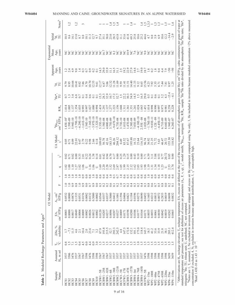
2.Modeled

RechargeParam

etersandAges

a

Sam

ple

Nam

eAssumed

Hr,m

asl

CEModel

UA

Model

c2

4He terr,

cm3STP/g

R/R

a

3He*,

TU

3H,

TU

Apparent

Age,

years

Exponential

Mean

Age,

years

Initial

3H,

TU

Notesb

Tr, �C

DNe,

%solubility

EA,

cm3STP/g

Ae,cm

3

STP/g

Fv

qc2

HCS1

3537

0.8

1.7

0.0003

0.0532

1.0

1.0

1.02

0.02

0.05

1.43E-10c

1.014

0.7

9.79

1.2

NC

10.5

HCS2

3506

1.5

�7.1

0.0000

0.0000

1.0

1.0

1.00

0.71

0.71

1.59E-09

1.005

1.3

8.95

2.4

NC

8.6

1,2

HCS3

3476

7.1

11.5

0.0017

0.0874

0.9

1.0

1.10

0.02

0.09

5.94E-10

1.137

3.4

10.66

4.9

NC

14.1

HCS4

3537

1.5

4.6

0.0049

0.1335

0.8

1.0

1.27

0.00

22.01

�3.79E-10

1.354

6.8

10.41

9.0

NC

13.0

1,2

HCS5

3567

0.4

2.1

0.0004

0.0531

1.0

1.0

1.02

0.33

0.47

�6.29E-10

1.035

0.7

8.02

1.4

NC

8.7

HCS6

3567

4.5

10.4

0.0009

0.0156

0.9

0.9

1.06

2.01

2.79

�1.61E-10

0.993

0.1

7.86

0.3

NC

8.0

3HCS7

3598

0.0

2.0

0.0002

0.0002

0.0

0.0

U0.22

0.22

1.54E-10

0.997

0.4

9.70

0.7

NC

10.1

HCS8

3476

4.4

23.6

0.0026

0.0132

0.7

0.8

1.16

0.24

0.98

�7.16E-10

1.027

0.6

10.70

0.9

NC

11.3

HCS9

3598

0.9

7.1

0.0012

0.5000

0.9

1.0

1.06

1.38

2.66

�3.97E-10

1.000

0.1

12.55

0.2

NC

12.7

HCS10

3598

3.0

3.2

0.0002

0.0002

0.0

0.0

U0.14

0.14

�3.32E-10

0.994

0.1

9.61

0.1

NC

9.7

HCSW1–5ft

3567

1.5

87.9

0.0120

0.0544

0.5

0.8

1.69

0.01

109.05

5.33E-10

1.419

15.3

12.17

14.5

NC

27.4

1HCBW1–25ft

3567

1.5

193.8

0.0205

0.0357

0.2

0.4

2.20

0.42

56.78

1.58E-08

1.291

28.3

6.87

29.0

16.7

35.1

1HCBW1–82ft

3567

1.5

215.5

0.0217

0.0337

0.2

0.4

2.28

0.94

42.16

4.00E-08

1.127

32.9

5.06

35.9

NC

38.0

1HCSW2–6ft

3537

1.5

52.7

0.0096

0.5000

0.6

1.0

1.52

0.70

183.13

3.75E-09

1.277

10.7

12.32

11.1

NC

23.0

1,4

HCBW2–38ft

3537

1.5

292.3

0.0287

0.0412

0.1

0.3

2.69

4.17

46.26

�9.67E-10

1.223

17.2

11.28

16.5

8.2

28.5

1,5

HCBW2–121ft

3537

1.5

242.5

0.0327

0.1001

0.2

0.7

2.87

0.00

204.12

6.73E-08

1.156

52.7

11.09

31.1

NC

63.8

1,4

HCCW3–5ft

3537

1.5

4.8

0.0009

0.1594

1.0

1.0

1.05

0.25

0.49

3.73E-10

1.048

1.5

9.59

2.5

NC

11.1

HCFW3–17ft

3537

1.5

147.5

0.0171

0.0404

0.3

0.6

1.99

1.29

83.52

1.01E-08

1.311

22.2

11.41

19.2

NC

33.6

1HCBW3–47ft

3537

1.5

172.8

0.0198

0.0421

0.2

0.5

2.15

0.15

87.67

1.47E-08

1.361

30.3

11.51

22.9

10.9

41.8

1HCBW3–157ft

3537

1.5

132.1

0.0200

0.1184

0.4

0.8

2.12

0.00

195.88

5.38E-08

1.351

54.9

14.40

27.9

NC

69.3

1,4

HCBW4–Int

3537

1.5

101.1

0.0106

0.0196

0.3

0.5

1.62

0.43

16.72

7.03E-09

1.241

14.5

11.33

14.6

7.6

25.8

1HCBW4–76ft

3537

1.0

175.0

0.0177

0.0273

0.2

0.4

2.03

0.10

23.64

�4.18E-10

1.024

1.5

9.12

2.7

NC

10.6

HCBW4–145ft

3537

1.5

118.4

0.0164

0.0690

0.4

0.8

1.93

0.00

116.35

2.55E–08

1.043

16.5

8.65

19.0

NC

25.2

1,4

HCFW5–5ft

3476

1.5

143.7

0.0171

0.0452

0.3

0.6

1.98

5.71

96.74

1.02E-08

1.451

29.0

15.56

18.7

9.0

44.6

1,5

WP2–15m

3598

1.5

18.5

0.0035

0.1603

0.8

1.0

1.19

6.39

36.92

�1.76E-10

1.014

0.5

4.23

1.8

NC

4.7

1,3,5

WP2–100ft

3598

1.5

41.2

0.0053

0.0212

0.6

0.8

1.31

3.11

21.25

�9.03E-11

0.998

0.1

7.92

0.2

NC

8.0

1WP2–60m

3598

1.5

33.6

0.0061

0.0815

0.7

0.9

1.34

5.88

71.72

1.12E�09

0.990

0.6

5.35

1.8

NC

5.9

1,5

WP2–475ft

3598

1.5

33.9

0.0030

0.0072

0.5

0.6

1.18

0.53

5.63

�6.45E-11

0.997

0.1

6.71

0.4

NC

6.9

1,3

WP2–650ft

3598

1.5

21.8

0.0042

0.2833

0.8

1.0

1.23

0.77

46.47

6.71E-09

0.973

3.2

7.44

6.4

NC

10.6

1WP2–220m

3598

1.5

38.1

0.0019

0.0019

0.0

0.0

U20.72

20.72

8.64E-09

0.981

4.3

7.81

7.9

NC

12.2

1,5

WP4–55m

3659

1.5

203.1

0.0262

0.0698

0.2

0.6

2.53

0.85

155.30

1.94E-07

0.258

�15.4

0.97

>50

NC

�14.4

1WP4–110m

3659

1.5

412.4

0.0465

0.0832

0.1

0.4

3.74

0.00

118.82

6.26E-07

0.228

�4.1

1.25

>50

NC

�2.9

1,4

aAbbreviationsareHr,rechargeelevation;Tr,rechargetemperature;EA,excess

airdefined

asthesum

oftheexcess

componentsofallatmosphericgases

(exceptHe);cm

3STP/g,cubiccentimeterspergram

ofwater

atstandardtemperature

andpressure;seetextfordefinitionofexcess

airparam

eters(A

e,F,v,

q);c2,model

misfit;

4He terr,terrigenic

4He;

R/R

a,sample

3He/4Heratiodivided

bytheatmospheric

3He/4Heratio;3He*,

tritiogenic

3He;

TU,tritium

unit;U,undefined;NC,notcomputed.

bNotesare1,Trassumed;2,Neexcluded

ininversionbecause

stripped,andexcess

airHecomponentcomputedusingNeonly;3,Heincluded

ininversionbecause

modeled

concentration>2%

abovemeasured

concentrationifexcluded;4,N2excluded

ininversionbecause

apparentdenitrification;5,c2unacceptably

high.

cRead1.43E-10as

1.43�

10�10.

W04404 MANNING AND CAINE: GROUNDWATER SIGNATURES IN AN ALPINE WATERSHED

9 of 16

W04404

sum of all modeled excess atmospheric gas components(including O2). Note that the EA composition is approxi-mately that of air, but not exactly because the CE model wasused instead of the unfractionated excess air (UA) model[Kipfer et al., 2002]. The Ne excess above solubility,expressed as DNe, traditionally has been used as a measureof excess air when the excess air is fractionated (as with theCE model) [Stute and Schlosser, 2000], so DNe is alsopresented for reference in Table 2. However, we believe thatEA is a more complete expression of excess air, and will useit henceforth. Excess air concentrations range from 0 to0.0465 cm3 STP/g, and consistently exceed 0.02 cm3 STP/g(DNe > 170%) in the bedrock HC wells and WP4. TheseEA concentrations are unusually high; typical concentra-tions are <0.01 cm3 STP/g (DNe < 100%) [Wilson andMcNeill, 1997; Stute and Schlosser, 2000]. The fact thatmany of the samples were collected with diffusion samplersrules out the possibility that the high EA concentrations aremerely the result of bubbles stuck in sampling tubes. Ingeneral, EA levels are lowest in the spring samples, higherin the shallow well samples, and highest in the bedrock wellsamples, suggesting a general trend of increasing EA withdepth (Figure 4), but this could be due in part to poorer gasconfinement in the shallower samples (see section 6).[29] Derived Ae values for bedrock samples are mainly

0.02–0.1 cm3 STP/g, similar to other reported values[Aeschbach-Hertig et al., 2000]. Unusually high EAvalues for the bedrock samples are due to unusually lowF values. The F parameter in the CE model is defined as F =v/q, where v is the fraction of the initial trapped gas volumeat the water table remaining after excess air entrainment(after equilibrium conditions are reestablished), and q is theratio of the dry gas pressure in the trapped gas to that inthe local atmosphere. The q parameter therefore indicatesthe magnitude of the water table rise responsible for theEA. The low F values are due primarily to unusually highq values that range mainly from 1.9 to 3.7, compared with1.1–1.6 for normal q values [Aeschbach-Hertig et al.,2000]. This range of modeled q values indicates watertable fluctuations of 3–15 m, which are large but well

within the range of observed water table fluctuations in theupper part of the watershed. The unusually large EAvalues observed in the bedrock aquifer are thereforeconsistent with the unusually large water table fluctuationsobserved in Handcart Gulch.[30] The large bedrock EA concentrations make this data

set an especially robust test of the CE model. Differencesbetween gas concentrations calculated using the UA and CEmodels generally become larger with increasing EA con-centrations, increasing the magnitude of misfit valuesresulting from application of an inappropriate model. Forbedrock samples, c2 values for the UA model are com-monly >40 (essentially 0% probability), whereas c2 valuesfor the CE model are generally acceptable (Table 2). Thepartial reequilibration (PR) model [Stute et al., 1995;Aeschbach-Hertig et al., 2000] was also applied to bedrockwell samples for comparison. Resulting c2 values weregenerally acceptable as with the CE model. Derived Ad

values (the amount of excess air initially dissolved) weremainly 0.05–0.10 cm3 STP/g, indicating water table fluc-tuations of 50–100 m. This range exceeds observed watertable fluctuations in the watershed but cannot be ruled out.Yet the PR model demands that 70–90% of the Ne initiallydissolved subsequently escaped by diffusion across thewater table for most of the bedrock samples. A simplecalculation was performed using Fick’s law to evaluate theplausibility of this scenario. Assumptions included (1) adiffusion distance of 10 m, a minimum based on Ad valuesand observed water table fluctuations; (2) a constant Neconcentration at the water table equal to solubility; and(3) a constant Ne concentration at 10 m below the water tableequal to the initial concentration indicated by Ad (an impos-sibility, but this results in maximum diffusion velocity).Under these conditions, about 100 years would be requiredto lose about 70% of the initial excess air Ne by diffusion,which is clearly problematic given downward average linearflow velocities �10 m/yr.[31] In contrast to the rest of the bedrock samples, EA

values for WP2 samples are not unusually high. This isunexpected given that the largest water table fluctuationswere observed in WP2. The well was drilled using streamwater (probably with low EA) 2 years prior to sampling. Itis probable that the well is still contaminated, particularly atdepths >160 m where thermal profiles indicate very lowflow rates (also see age results in section 5.3). However, thisseems unlikely at shallower depths where thermal profilesand flowmeter data indicate active flow, particularly at<50 m in the zone of annual water table fluctuation.Resampling the well in the future might help explain theapparent conflict.

5.3. 3H/3He Ages

[32] Apparent 3H/3He ages [Schlosser et al., 1988, 1989]range from 0.1 to 35.9 years (Table 2) and generally have anuncertainty of 0.5–2.0 years. Initial 3H values (measured3H + measured tritiogenic 3He) were compared with theprecipitation 3H record (input curve) to evaluate the possi-bility that the samples contain a significant fraction of waterrecharge prior to 1950 (prebomb water) (Figure 5a). On aplot of initial 3H versus apparent 3H/3He recharge year,samples should plot close to the input curve; samplesplotting significantly below it probably have a significant

Figure 4. Box-whisker plot comparing excess air con-centrations in spring samples, shallow well samples, andbedrock well samples. Excess air is the sum of the modeledexcess atmospheric gas components.

10 of 16

W04404 MANNING AND CAINE: GROUNDWATER SIGNATURES IN AN ALPINE WATERSHED W04404

component of prebomb water [Stute et al., 1997; Aeschbach-Hertig et al., 1998; Manning et al., 2005]. For samplesplotting below the input curve, the apparent 3H/3He age isonly representative of the fraction of the sample rechargedafter 1950 (modern fraction). The three closest availableprecipitation 3H records were from Denver, Colorado, SaltLake City, Utah, and Albuquerque, New Mexico [Interna-tional Atomic Energy Agency, 2006]. The Denver record wastoo short (1963–1968) to allow construction of a reliablecomplete record by correlation. Complete records wereconstructed for Salt Lake City and Albuquerque by correla-

tion with Ottawa and Vienna records as described byManning et al. [2005] (Figure 5a).[33] Although both records are shown on Figure 5a for

comparison, we believe precipitation 3H at the site moreclosely matches the Salt Lake City record than the Albu-querque because (1) initial 3H values for samples withapparent ages <5 years (least likely to contain prebombwater) plot closer to the Salt Lake City record (Figure 5b);and (2) for those years in which Denver precipitationconcentrations are available, they are closer to Salt LakeCity concentrations. The Salt Lake City record was there-fore used to evaluate the presence of prebomb water and tocompute exponential ages and will be henceforth referred toas the input curve for the site. Most samples plot relativelyclose to the input curve (Figure 5a), indicating that theycontain little prebomb water. The exceptions are the threesamples with the oldest apparent ages, HCBW1–82ft,HCBW1–25ft, and HCBW2–121ft. Of these, HCBW1–82ft probably contains the most prebomb water (and thushas the oldest residence time), followed by HCBW1–25ftand then HCBW2–121ft. Samples from WP2 are excludedfrom Figure 5 and from all following figures in whichapparent age is plotted because of previously mentionedconcerns about drilling water contamination. Notably absentin Figure 5 are mixtures of very old and very young waterthat might be expected in a highly heterogeneous flowsystem.[34] Mean groundwater ages for the integrated bedrock

well samples were computed from their apparent ages usingthe 3H input curve assuming that these samples contain anexponential age distribution [Vogel, 1967; Cook and Bohlke,2000] (Table 2). A curve indicating expected initial 3Hvalues for samples with exponential age distributions wasalso computed (Figure 5a). This curve is close to asmoothed version of the input curve but is slightly aboveit for recharge years in the 1980s. Initial 3H values for fourof the five integrated samples, all with recharge years in the1980s, also plot slightly above the input curve, relativelyclose to the exponential curve. HCBW1–25ft is the excep-tion, plotting well below the exponential curve. 3H and 3Heconcentrations in four of the five integrated samples aretherefore consistent with exponential age distributions.[35] Apparent ages from springs and HC wells are plotted

relative to distance down the stream in Figure 6. Springsample ages are the youngest (mainly <3 years), followed byshallow well samples (11–19 years) and then bedrock wellsamples (mainly 15–36 years). Discrete bedrock samplescollected from near the bottom of the bedrock HC wellshave the oldest apparent ages in each location. The apparentages along with initial 3H (Figure 5a) and terrigenic Heconcentrations (Table 2) all indicate that groundwater agesin the vicinity of the stream increase with depth. TerrigenicHe (Heterr) is the component of He, other than tritiogenic He,with a nonatmospheric source, most likely some combina-tion of U-Th series decay in crustal rocks and diffusion fromthe mantle. Because of its subsurface source, Heterr typicallyincreases with age [Solomon, 2000]. Exponential mean agesfor the integrated samples are also shown. Exponential meanages from HC2 to HC5 are remarkably uniform, rangingfrom 8 to 11 years. The 3H and He data are thereforegenerally consistent with a uniform flow system down-stream of HC2, which includes most of the site. Note that

Figure 5. Apparent recharge year (from apparent 3H/3Heage) versus sample initial 3H concentration (measured 3H +tritiogenic 3He). Precipitation 3H records for Salt Lake City,Utah (SLC precip) and Albuquerque, New Mexico (Albprecip), constructed from mean annual average concentra-tions, are shown for comparison. (a) All samples. A curverepresenting expected initial 3H concentrations for sampleswith an exponential age distribution (SLC exp), calculatedfrom the Salt Lake City record, is also shown for comparisonwith integrated bedrock well samples (int BR sample).Labeled samples are 1, HCBW1–82ft; 2, HCBW2–121ft;3, HCBW1–25ft. (b) Samples with apparent ages <5 years.A point representing the average of these samples is alsoshown.

W04404 MANNING AND CAINE: GROUNDWATER SIGNATURES IN AN ALPINE WATERSHED

11 of 16

W04404

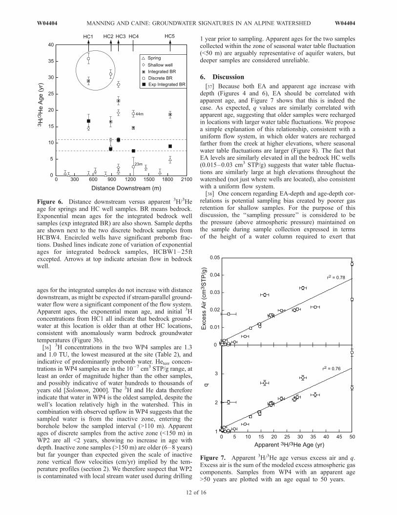
ages for the integrated samples do not increase with distancedownstream, as might be expected if stream-parallel ground-water flow were a significant component of the flow system.Apparent ages, the exponential mean age, and initial 3Hconcentrations from HC1 all indicate that bedrock ground-water at this location is older than at other HC locations,consistent with anomalously warm bedrock groundwatertemperatures (Figure 3b).[36] 3H concentrations in the two WP4 samples are 1.3

and 1.0 TU, the lowest measured at the site (Table 2), andindicative of predominantly prebomb water. Heterr concen-trations in WP4 samples are in the 10�7 cm3 STP/g range, atleast an order of magnitude higher than the other samples,and possibly indicative of water hundreds to thousands ofyears old [Solomon, 2000]. The 3H and He data thereforeindicate that water in WP4 is the oldest sampled, despite thewell’s location relatively high in the watershed. This incombination with observed upflow in WP4 suggests that thesampled water is from the inactive zone, entering theborehole below the sampled interval (>110 m). Apparentages of discrete samples from the active zone (<150 m) inWP2 are all <2 years, showing no increase in age withdepth. Inactive zone samples (>150 m) are older (6–8 years)but far younger than expected given the scale of inactivezone vertical flow velocities (cm/yr) implied by the tem-perature profiles (section 2). We therefore suspect that WP2is contaminated with local stream water used during drilling

1 year prior to sampling. Apparent ages for the two samplescollected within the zone of seasonal water table fluctuation(<50 m) are arguably representative of aquifer waters, butdeeper samples are considered unreliable.

6. Discussion

[37] Because both EA and apparent age increase withdepth (Figures 4 and 6), EA should be correlated withapparent age, and Figure 7 shows that this is indeed thecase. As expected, q values are similarly correlated withapparent age, suggesting that older samples were rechargedin locations with larger water table fluctuations. We proposea simple explanation of this relationship, consistent with auniform flow system, in which older waters are rechargedfarther from the creek at higher elevations, where seasonalwater table fluctuations are larger (Figure 8). The fact thatEA levels are similarly elevated in all the bedrock HC wells(0.015–0.03 cm3 STP/g) suggests that water table fluctua-tions are similarly large at high elevations throughout thewatershed (not just where wells are located), also consistentwith a uniform flow system.[38] One concern regarding EA-depth and age-depth cor-

relations is potential sampling bias created by poorer gasretention for shallow samples. For the purpose of thisdiscussion, the ‘‘sampling pressure’’ is considered to bethe pressure (above atmospheric pressure) maintained onthe sample during sample collection expressed in termsof the height of a water column required to exert that

Figure 6. Distance downstream versus apparent 3H/3Heage for springs and HC well samples. BR means bedrock.Exponential mean ages for the integrated bedrock wellsamples (exp integrated BR) are also shown. Sample depthsare shown next to the two discrete bedrock samples fromHCBW4. Encircled wells have significant prebomb frac-tions. Dashed lines indicate zone of variation of exponentialages for integrated bedrock samples, HCBW1–25ftexcepted. Arrows at top indicate artesian flow in bedrockwell.

Figure 7. Apparent 3H/3He age versus excess air and q.Excess air is the sum of the modeled excess atmospheric gascomponents. Samples from WP4 with an apparent age>50 years are plotted with an age equal to 50 years.

12 of 16

W04404 MANNING AND CAINE: GROUNDWATER SIGNATURES IN AN ALPINE WATERSHED W04404

pressure. Downhole total dissolved gas pressure probereadings from bedrock HC wells (Table 1) indicate thatsampling pressures of at least 5 m are generally required toassure full gas retention for bedrock groundwaters. There-fore several samples may have lost gas, including springsamples (sampling pressure essentially = 0 m), bailedsamples (sampling pressure = 1–2 m), and samples collectedwith diffusion samplers at depths <5 m (Table 1). The firstscenario of concern is that all samples originally had highEA levels, but samples collected at progressively shallowerdepths (lower sampling pressures) lost progressively moregas, leading to an apparent EA-depth correlation. Thisscenario cannot be ruled out for the spring samples; theyhave both the lowest sampling pressures and the lowestaverage EA (Figure 9). Bubbles were observed in the springpool during collection of sample HCS4, the spring withthe highest modeled EA, indicating that gas was indeedprobably lost from this sample. However, well sampleswith low sampling pressures, including bailed samples anddiffusion samplers collected at depths <2 m, are notconsistent with this scenario. If EA values were mainlycontrolled by sampling pressure, then these samples shouldall have similar EA values that fall mainly between thoseof spring samples and those of well samples having highsampling pressures (>5 m). Instead, they have EA valuesthat span nearly the entire range for the site (Figure 9). Ittherefore appears that although spring samples are probablyincapable of preserving high EA levels like those in thebedrock aquifer, sample pressures >1 m are (at leastpartially), and the EA-depth correlation cannot be com-pletely explained by sampling bias.[39] The second scenario of concern is that all samples

originally had apparent ages similar to the bedrock wellsamples (>15 years), and samples collected at shallowerdepths have younger ages only due to gas loss. Gas loss willdecrease apparent ages through the loss of tritiogenic 3Heand by decreasing measured 3He/4He ratios as a result offractionation between exsolved bubbles and the remaining

fluid. Potential changes in apparent ages due to gas losswere computed for the integrated bedrock samples assum-ing loss of the entire excess air component of He (worst-case scenario). Apparent ages do drop significantly to the5- to 10-year range but still remain above the apparent agesof most spring samples (<2 years) because their consistentlyhigher 3He/4He ratios (R/Ra in Table 2) are largely pre-served. Therefore the age-depth correlation can be onlypartly explained by degassing.[40] If varying degrees of gas loss were the main cause of

observed variations in EA and age, and thus the EA-agecorrelation, then samples with similar sampling pressuresshould exhibit little or no correlation between EA andapparent age. Figure 10 demonstrates that this is not thecase for spring samples and well samples with low samplingpressures, both sample types exhibiting a clear EA-agecorrelation. A final argument against significant gas lossis the fact that gas concentrations generally fit the CE modelwell. If degassing had occurred, one would expect afractionation pattern that could not be described by theCE model.[41] The most distinctive characteristics of dissolved

gases in the Handcart Gulch bedrock aquifer are theunusually high EA concentrations and the correlationbetween EA and age. An important question is whetheror not these characteristics are typical of alpine bedrockaquifers. Other dissolved gas data collected in the moun-tains exhibit normal EA concentrations of <0.01 cm3 STP/g[Manning et al., 2003; Rademacher et al., 2001; Holocheret al., 2001; Plummer et al., 2001; Rauber et al., 1991;Zuber et al., 1995; Mazor et al., 1983], with only a fewexceptional samples [Rademacher et al., 2001; Mazor et al.,

Figure 8. Cross section showing proposed explanation forcorrelation between q and apparent 3H/3He age.

Figure 9. Box-whisker plot comparing excess air con-centrations in spring samples, samples with low samplingpressure (<5 m), and samples with high sampling pressure(>5 m). Sampling pressure is the pressure (above atmo-spheric pressure) maintained on the sample during samplecollection expressed in terms of the height of a watercolumn required to exert that pressure. P means pressure.Excess air is the sum of the modeled excess atmospheric gascomponents.

W04404 MANNING AND CAINE: GROUNDWATER SIGNATURES IN AN ALPINE WATERSHED

13 of 16

W04404

1983]. However, these data have generally been collectedfrom (1) springs, which probably cannot preserve high EAconcentrations; (2) shallow alluvial wells, which may notintercept bedrock waters; or (3) environments that aremountainous but not alpine. Dissolved gas data presentedby Johnson et al. [2007] are an important exception. Thesedata were collected from Prospect Gulch, an alpine water-shed in the San Juan Mountains of Colorado at elevations>3100 m asl. Samples were collected from springs and wellscompleted at different depths, including a bedrock welllocated near the trunk stream at the bottom of the watershed.As in Handcart Gulch, the bedrock well is artesian, andsamples from different depths in the well (27–41 m) haveunusually high EA (DNe > 200%). Bedrock wells higher inthe watershed also show large water table fluctuationssimilar to those observed at Handcart Gulch. We thereforesuspect that the high EA levels found in Handcart Gulch maybe typical for alpine bedrock aquifers, and the primaryreason they have not been found elsewhere is a lack ofbedrock wells in alpine watersheds.[42] A correlation between apparent tracer age and EA

has been observed in other mountain settings [Plummer etal., 2001; Manning et al., 2003, Figure 4b]. Figure 11shows modeled EA (expressed as DNe) plotted versusapparent 3H/3He ages for the previously described alpinegroundwater samples presented by Johnson et al. [2007].Samples with low sampling pressures (<1 m) and samples

with higher sampling pressures (>2 m) are plotted separatelybecause gas loss is a concern, as at Handcart Gulch. EA andapparent age are clearly correlated, and the fact they arecorrelated for both sample types demonstrates that thecorrelation is not due to gas loss alone. Therefore we suspectthat higher EA concentrations are commonly associated witholder waters in alpine watersheds.[43] In Handcart Gulch, the exponential mean ages for the

integrated samples and the apparent ages of the springsamples imply a mean residence time of 8–11 years formost of the bedrock groundwater and <2 years for most ofthe shallow groundwater system feeding the springs. Thesemean residence times are similar to those calculated fordeep/bedrock groundwater (5–9 years) and shallow ground-water (1–3 years) in other mountain watersheds usinglumped parameter modeling [Uhlenbrook et al., 2002;Maloszewski et al., 1983; Soulsby et al., 2000]. It shouldbe understood that all mean residence times for fracturedbedrock aquifers calculated from environmental tracer datamay be older than the true mean residence time of the waterdue to diffusive exchange of the tracer between mobilefracture water and more immobile matrix water [e.g., Cooket al., 2005]. For the purposes of this paper, however,relative age, not absolute age, is of primary importance.

7. Conclusions

[44] 1. Temperature profiles indicate active groundwatercirculation to a maximum depth (aquifer thickness) of about200 m, or about 150 m below the water table. Boreholetemperature logging is a reliable method of identifyingaquifer thickness in alpine watersheds underlain by frac-tured crystalline rock because linear profiles with slopessimilar to the conductive geothermal gradient are reliable

Figure 10. Apparent 3H/3He age versus excess air for(a) spring samples and (b) samples with low samplingpressures (<5 m). Excess air is the sum of the modeledexcess atmospheric gas components. Samples from WP4with an apparent age >50 years are plotted with an age equalto 50 years.

Figure 11. Apparent 3H/3He age versus excess airexpressed as DNe for samples from Prospect Gulch,Colorado, from Johnson et al. [2007]. Separate linearregression lines are shown for samples with samplingpressures <1 m (dashed line) and >1 m (solid line).

14 of 16

W04404 MANNING AND CAINE: GROUNDWATER SIGNATURES IN AN ALPINE WATERSHED W04404

indicators of very low flow velocities characteristic of theunderlying inactive zone.[45] 2. Dissolved noble gas data show unusually high

excess air concentrations (>0.02 cm3 STP/g, DNe > 170%)in the bedrock, consistent with unusually large seasonalwater table fluctuations (up to 50 m) observed in the upperpart of the watershed. Dissolved gases are fractionated andsupport the CE model of excess air formation.[46] 3. Apparent 3H/3He ages are positively correlated

with sample depth and excess air concentrations. Althoughspring samples have probably experienced gas loss, thecorrelation cannot be attributed mainly to sampling bias.Most of the EA-age correlation is probably due to watertable fluctuations increasing with distance from the stream.[47] 4. Exponential mean ages for integrated bedrock well

samples, assumed to be approximately flow weighted due toartesian flow, are remarkably consistent along the stream,four of five being from 8 to 11 years. This result incombination with other hydrologic and geologic data sup-ports a simple watershed-scale conceptual model of ground-water flow in which permeability is primarily a function ofdepth and where recharge, aquifer thickness, and porosityare relatively uniform throughout most of the watershed.This result is surprising given the complexity of the bedrockgeology. A flow system of this sort could be reasonably wellrepresented with an equivalent porous media model cali-brated with limited data, and such a model may yield usefulinformation about solute transport and chemical mass bal-ance within the watershed.

[48] Acknowledgments. This work was funded by the U.S. Geolog-ical Survey’s Mendenhall Post-doctoral Research Fellowship Program,Mineral Resources Program within the Geologic Discipline, and ToxicsProgram within the Water Resources Discipline. We thank CharlesRobinson of Mineral Systems, Inc., for graciously donating the deepboreholes to the USGS. We also thank the U.S. Forest Service and theColorado Geological Survey for their cooperation. Reviews by WernerAeschbach-Hertig, Peter McMahon, and Bert Stolp were very helpful andimproved the manuscript.

ReferencesAeschbach-Hertig, W., P. Schlosser, M. Stute, H. J. Simpson, A. Ludin, andJ. F. Clark (1998), A 3H/3He study of ground water flow in a fracturedbedrock aquifer, Ground Water, 36, 661–670.

Aeschbach-Hertig, W., F. Peeters, U. Beyerle, and R. Kipfer (1999), Inter-pretation of dissolved atmospheric noble gases in natural waters, WaterResour. Res., 35, 2779–2792.

Aeschbach-Hertig, W., F. Peeters, U. Beyerle, and R. Kipfer (2000), Paleo-temperature reconstruction from noble gases in ground water taking intoaccount equilibration with entrapped air, Nature, 405, 1040–1043.

Ballentine, C. J., and C. M. Hall (1999), Determining paleotemperature andother variables by using an error-weighted, nonlinear inversion of noblegas concentrations in water, Geochim. Cosmochim. Acta, 63, 2315–2336.

Bayer, R., P. Schlosser, G. Bonisch, H. Rupp, F. Zaucker, and G. Zimmek(1989), Performance and blank components of a mass spectrometric sys-tem for routine measurement of helium isotopes and tritium by the 3Heingrowth method, in Sitzungsberichte der Heidelberger Akademie derWissenschaften, Mathematisch-Naturwissenschaftliche Klasse, vol. 5,pp. 241–279, Springer, New York.

Birch, F. (1950), Flow of heat in the Front Range, Colorado, Geol. Soc. Am.Bull., 61, 567–630.

Bossong, C. R., J. S. Caine, D. I. Stannard, J. L. Flynn, M. R. Stevens, andJ. S. Heiny-Dash (2003), Hydrologic conditions and assessment of waterresources in the Turkey Creek Watershed, Jefferson County, Colorado,1998–2001,U.S. Geol. Surv. Water Resour. Invest. Rep., 03-4034, 140 pp.

Bredehoeft, J. D., and I. S. Papadopulos (1965), Rates of vertical ground-water movement estimated from the Earth’s thermal profile, Water Re-sour. Res., 1, 325–328.

Burns, D. A., P. S. Murdoch, G. B. Lawrence, and R. L. Michel (1998),Effect of groundwater springs on NO3

� concentrations during summer inCatskill Mountain streams, Water Resour. Res., 34, 1987–1996.

Caine, J. S., and S. R. A. Tomusiak (2003), Brittle structures and their rolein controlling porosity and permeability in a complex Precambrian crys-talline-rock aquifer system in the Colorado Rocky Mountain FrontRange, Geol. Soc. Am. Bull., 115, 1410–1424.

Caine, J. S., A. H. Manning, P. L. Verplanck, D. J. Bove, K. G. Kahn, andS. Ge (2006), Well construction information, lithologic logs, water leveldata, and overview of research in Handcart Gulch, Colorado: An alpinewatershed affected by metalliferous hydrothermal alteration, U.S. Geol.Surv. Open File Rep., 06-1189, 14 pp.

Cook, P. G., and J. K. Bohlke (2000), Determining timescales for ground-water flow and solute transport, in Environmental Tracers in SubsurfaceHydrology, edited by P. G. Cook and A. L. Herczeg, pp. 1–30, Springer,New York.

Cook, P. G., A. J. Love, N. I. Robinson, and C. T. Simmons (2005),Groundwater ages in fractured rock aquifers, J. Hydrol., 308, 284–301.

Decker, E. R. (1969), Heat flow in Colorado and New Mexico, J. Geophys.Res., 74, 550–559.

Dekay, R. H. (1972), Development of ground-water supplies in ShenandoahNational Park, Virginia,Rep. 10, Va.Div. ofMiner. Resour., Charlottesville.

Desbarats, A. J. (2002), A lumped-parameter model of groundwater influxto a mine adit in mountainous terrain, Water Resour. Res., 38(11), 1256,doi:10.1029/2001WR001058.

Diersch, H.-J. D. (1998), FEFLOW: Reference manual—Release 4.7,WASY, Berlin.

Domenico, P. A., and V. V. Palciauskas (1973), Theoretical analysis offorced convective heat transfer in regional ground-water flow, Geol.Soc. Am. Bull., 84, 3803–3814.

Ferguson, G., H. Beltrami, and A. D. Woodbury (2006), Perturbation ofground surface temperature reconstructions by groundwater flow?, Geo-phys. Res. Lett., 33, L13708, doi:10.1029/2006GL026634.

Forster, C., and L. Smith (1989), The influence of groundwater flow onthermal regimes in mountainous terrain: A model study, J. Geophys.Res., 94, 9439–9451.

Guan, H. (2005), Water above the mountain front—Assessing mountain-block recharge in semiarid regions, Ph.D. thesis, N. M. Inst. of Miningand Technol., Soccoro.

Haitjema, H. M. (1995), On the residence time distribution in idealizedgroundwatersheds, J. Hydrol., 172, 127–146.

Heaton, T. H. E., and J. C. Vogel (1981), ‘‘Excess air’’ in groundwater,J. Hydrol., 50, 201–216.

Hely, A. G., R. W. Mower, and C. A. Harr (1971), Water resources of SaltLake County, Utah, Tech. Publ. 31, Utah Dep. of Nat. Resour., Salt LakeCity.

Herrmann, A., and W. Stichler (1980), Groundwater-runoff relationships,Catena, 7, 251–264.

Holocher, J., V. Matta, W. Aeschbach-Hertig, U. Beyerle, M. Hofer,F. Peeters, and R. Kipfer (2001), Noble gas and major element constraintson thewater dynamics in an alpine floodplain,GroundWater, 39, 841–852.

International Atomic Energy Agency (2006), Isotope Hydrology Sectiondatabase, Vienna. (Available at http://isohis.iaea.org)

Johnson, R. H., L. Wirt, R. R. McDougal, A. H. Manning, D. B. Yager,D. L. Fey, and K. J. Leib (2007), Geochemistry of surface and groundwater in Cement Creek from Gladstone to Georgia Gulch and in Pro-spect Gulch, San Juan County, Colorado, U.S. Geol. Surv. Open File.Rep., 07-1004.

Kahn, K. G. (2005), Analysis of the shallow groundwater system in analpine basin: Handcart Gulch, Colorado, M.S. thesis, 148 pp., Univ. ofColo., Boulder.

Kimball, B. A., R. L. Runkel, and L. J. Gerner (2001), Quantification ofmine drainage inflows to Little Cottonwood Creek, Utah, using a tracer-injection and synoptic-sampling study, Environ. Geol., 40, 1390–1404.

Kimball, B. A., R. L. Runkel, K. Walton-Day, and K. Bencala (2002),Assessment of metal loads in watersheds affected by acid mine drainageby using tracer injection and synoptic sampling: Cement Creek, Color-ado, USA, Appl. Geochem., 17, 1183–1207.

Kipfer, R., W. Aeschbach-Hertig, F. Peeters, and M. Stute (2002), Noblegases in lakes and ground waters, in Reviews in Mineralogy and Geo-chemsitry, vol. 47, Noble Gases in Geochemistry and Cosmochemistry,edited by D. Porcelli et al., pp. 615–700, Mineral. Soc. of Am.,Chantilly, Va.

Kosugi, K., S. Katsura, M. Katsuyama, and T. Mizuyama (2006), Waterflow processes in weathered granitic bedrock and their effects on runoffgeneration in a small headwater catchment, Water Resour. Res., 42,W02414, doi:10.1029/2005WR004275.

W04404 MANNING AND CAINE: GROUNDWATER SIGNATURES IN AN ALPINE WATERSHED

15 of 16

W04404

Liu, F., M. W. Williams, and N. Caine (2004), Source waters and flow pathsin an alpine catchment, Colorado Front Range, United States, WaterResour. Res., 40, W09401, doi:10.1029/2004WR003076.

Lovering, T. S. (1935), Geology and ore deposits of the Montezuma Quad-rangle, Colorado, U.S. Geol. Surv. Prof. Pap., 178, 119 pp.

Maloszewski, P., and A. Zuber (1982), Determining the turnover time ofgroundwater systems with the aid of environmental tracers: 1. Modelsand their applicability, J. Hydrol., 57, 207–231.

Maloszewski, P., W. Rauert, W. Stichler, and A. Herrmann (1983), Appli-cation of flow models in an alpine catchment area using tritium anddeuterium data, J. Hydrol., 66, 319–330.

Manning, A. H., and D. K. Solomon (2004), Constraining mountain-blockrecharge to the eastern Salt Lake Valley, Utah, with dissolved noble gasand tritium data, in Groundwater Recharge in a Desert Environment: TheSouthwestern United States, Water Sci. Appl. Ser., vol. 9, edited by J. F.Hogan et al., pp. 139–158, AGU, Washington, D. C.

Manning, A. H., and D. K. Solomon (2005), An integrated environmentaltracer approach to characterizing groundwater circulation in mountainblock, Water Resour. Res., 41, W12412, doi:10.1029/2005WR004178.

Manning, A. H., D. K. Solomon, and A. L. Sheldon (2003), Applications ofa total dissolved gas pressure probe in ground water studies, GroundWater, 41, 440–448.

Manning, A. H., D. K. Solomon, and S. A. Thiros (2005), 3H/3He age datain assessing the susceptibility of wells to contamination, Ground Water,43, 353–367.

Marechal, J. C. (1999), Observation des massifs cristallins alpins au traversdes ouvrages souterrains: 2. Definition du role hydrogeologique de lazone decomprimee, Hydrogeologie, 2, 33–42.

Marechal, J. C., and D. Etcheverry (2003), The use of 3H and 18O tracers tocharacterize water inflows in Alpine tunnels, Appl. Geochem., 18, 339–351.

Mau, D. P., and T. C. Winter (1997), Estimating ground-water recharge andbaseflow from streamflow hydrographs for a small watershed in NewHampshire, Ground Water, 35, 291–304.

Mayo, A. L., and W. Koontz (2000), Fracture flow and groundwater com-partmentalization in the Rollins Sandstone, Lower Mesaverde Group,Colorado, USA, Hydrogeol. J., 8, 430–446.

Mayo, A. L., T. H. Morris, S. Peltier, E. C. Petersen, K. Payne, L. S.Holman, D. Tingey, T. Fogel, B. J. Black, and T. D. Gibbs (2003), Activeand inactive groundwater flow systems: Evidence from a stratified,mountainous terrain, Geol. Soc. Am. Bull., 115, 1456–1472.

Mazor, E., R. O. van Everdingen, and H. R. Krouse (1983), Noble-gasevidence for geothermal activity in a karstic terrain: Rocky Mountains,Canada, Geochim. Cosmochim. Acta, 47, 1111–1115.

Mendoza, G. F., T. S. Steenhuis, M. T. Walter, and J. Y. Parlange (2003),Estimating basin-wide hydraulic parameters of a semi-arid mountainouswatershed by recession-flow analysis, J. Hydrol., 279, 57–69.

Mulholland, P. J. (1993), Hydrometric and stream chemistry evidence ofthree storm flowpaths in Walker Branch Watershed, J. Hydrol., 151,291–316.

Plummer, L. N., E. Busenberg, J. K. Bohlke, D. L. Nelms, R. L. Michel,and P. Schlosser (2001), Groundwater residence times in ShenandoahNational Park, Blue Ridge Mountains, Virginia, USA: A multi-tracerapproach, Chem. Geol., 179, 93–111.

Polyakov, V. A., S. A. Medvedev, and N. V. Pyatnitskij (1996), An isotopicand hydrochemical study of the groundwater inflow into the north-Muyatunnel, in Isotopes in Water Resource Management: Proceedings of aSymposium on Water Resources Management, Int. At. Energy Agency,Vienna.

Rademacher, L. K., J. F. Clark, G. B. Hudson, D. C. Erman, and N. A.Erman (2001), Chemical evolution of shallow groundwater as recordedby springs, Sagehen basin, Nevada County, California, Chem. Geol., 179,37–51.

Rademacher, L. K., J. F. Clark, and J. R. Boles (2003), Groundwaterresidence times and flow paths in fractured rock determined using en-vironmental tracers in the Mission Tunnel, Santa Barbara County, Cali-fornia, USA, Environ. Geol., 43, 557–567.

Rahn, P. H. (1981), Ground water stored in the rocks of western SouthDakota, in Geology of the Black Hills, South Dakota and Wyoming, FieldTrip Guide Book, Geological Society of America, edited by F. J. Rich,pp. 154–173, Am. Geol. Inst., Alexandria, Va.

Rauber, D., H. H. Loosli, H. Schmassmann, and J. N. Andrews (1991),Noble gases in groundwater, in Applied Isotope Hydrogeology: A CaseStudy in Northern Switzerland, Stud. Environ. Sci. Ser., vol. 43, edited byF. J. Pearson et al., pp. 117–149, Elsevier, New York.

Robinson, C. S. (1978), Hydrology of fractured crystalline rocks, Hender-son Mine, Colorado, Min. Eng., 30, 1185–1194.

Robinson, C. S., F. T. Lee, J. H. Scott, R. D. Carroll, R. T. Hurr, D. B.Richards, F. A. Mattei, B. E. Hartmann, and J. F. Abel (1974), Engineer-ing geologic, geophysical, hydrologic and rock-mechanics investigationsof the Straight Creek Tunnel site and pilot bore, Colorado, U.S. Geol.Surv. Prof. Pap., 815, 134 pp.

Runkel, R. L., B. A. Kimball, K. Walton-Day, and P. L. Verplanck (2003),When good tracers go bad: Tracer-dilution sausage recipes revealed, EosTrans. AGU, 84(46), Fall Meet. Suppl., Abstract H51C-1044.

Sanford, W. E., R. G. Shropshire, and D. K. Solomon (1996), Dissolved gastracers in groundwater: Simplified injection, sampling, and analysis,Water Resour. Res., 32, 1635–1642.

Schlosser, P., M. Stute, H. Dorr, C. Sonntag, and K. O. Munnich (1988),Tritium/3He dating of shallow groundwater, Earth Planet. Sci. Lett., 89,353–362.

Schlosser, P., M. Stute, C. Sonntag, and K. O. Munnich (1989), Tritiogenic3He in shallow groundwater, Earth Planet. Sci. Lett., 94, 245–256.

Snow, D. T. (1973), Mountain groundwater supplies, Mountain Geol., 10,19–24.

Solomon, D. K. (2000), 4He in groundwater, in Environmental Tracers inSubsurface Hydrology, edited by P. G. Cook and A. L. Herczeg, pp. 425–439, Springer, New York.

Soulsby, C., R. Malcolm, and I. Malcolm (2000), Groundwater in head-waters: Hydrological and ecological significance, Geol. Soc. Spec. Publ.,182, 19–34.

Stute, M. and P. Schlosser (2000), Atmospheric noble gases, in Environ-mental Tracers in Subsurface Hydrology, edited by P. G. Cook and A. L.Herczeg, pp. 349–377, Springer, New York.

Stute, M., M. Forster, H. Frischkorn, A. Serejo, J. F. Clark, P. Schlosser,W. S. Broeker, and G. Bonani (1995), Cooling of tropical Brazil (5�C)during the Last Glacial Maximum, Science, 269, 379–383.

Stute, M., J. Deak, K. Revesz, J. K. Boehlke, E. Deseoe, R. Weppernig, andP. Schlosser (1997), Tritium/3He dating of river infiltration: An examplefrom the Danube in the Szigetkoez area, Hungary, Ground Water, 35,905–911.

Sueker, J., J. N. Ryan, C. Kendall, and R. D. Jarrett (2000), Determinationof hydrologic pathways during snowmelt for alpine/subalpine basins,Rocky Mountain National Park, Colorado, Water Resour. Res., 36,63–75.

Tiedeman, C. R., D. J. Goode, and P. A. Hsieh (1998), Characterizing aground water basin in a New England mountain and valley terrain,Ground Water, 36, 611–620.

Todd, A., and D. McKnight (2003), Abandoned mines, mountain sports,and climate variability: Implications for the Colorado tourism economy,Eos Trans. AGU, 84(38), 377386.

Uhlenbrook, S., M. Frey, C. Leibundgut, and P. Maloszewski (2002), Hy-drograph separations in a mesoscale mountainous basin at event andseasonal timescales, Water Resour. Res., 38(6), 1096, doi:10.1029/2001WR000938.

VanderBeek, G. A. (2003), Estimating recharge and storage coefficient in afractured rock aquifer, Turkey Creek Basin, Jefferson County, Colorado,M.S. thesis, 115 pp., Colo. School of Mines, Golden.

Vogel, J. C. (1967), Investigation of groundwater flow with radiocarbon,in Isotopes in Hydrology, Rep. IAEA-SM-83/7, pp. 355–369, Int. At.Energy Agency, Vienna.

Wasiolek, M. (1995), Subsurface recharge to the Tesuque Aquifer systemfrom selected drainage basins along the western side of the Sangre deCristo Mountains near Santa Fe, New Mexico, U.S. Geol. Surv. WaterResour. Invest. Rep., 94–4072, 57 pp.

Wilson, J. L., and H. Guan (2004), Mountain-block hydrology and moun-tain-front recharge, in Groundwater Recharge in a Desert Environment:The Southwestern United States, Water Sci. Appl. Ser., vol. 9, edited byJ. F. Hogan et al., pp. 113–137, AGU, Washington, D. C.

Wilson, G. B., and G. W. McNeill (1997), Noble gas recharge temperaturesand the excess air component, Appl. Geochem., 12, 747–762.

Zecharias, Y. B., and W. Brutsaert (1988), Recession characteristics ofgroundwater outflow and baseflow from mountainous watersheds, WaterResour. Res., 24, 1651–1658.

Zuber, A., S. M. Weise, K. Osenbruck, J. Grabczak, and W. Ciezkowski(1995), Age and recharge area of thermal waters in Ladek Spa (Sudeten,Poland) deduced from environmental isotope and noble gas data,J. Hydrol., 167, 327–349.

����������������������������J. S. Caine and A. H. Manning, U.S. Geological Survey, P.O. Box

25046, Mail Stop 964, Denver, CO 80225, USA. (amanning@usgs.gov)

16 of 16

W04404 MANNING AND CAINE: GROUNDWATER SIGNATURES IN AN ALPINE WATERSHED W04404