CLASSIFICATIONS OF ACCURACY AND STANDARDS … · performed by Caltrans or others on all Caltrans-involved transportation improvement projects will be classified according to the standards

CLASSIFICATIONS OF ACCURACY AND STANDARDS April 2015

5 Classifications of Accuracy and Standards

Contents 5.1 Introduction ....................................................................................................................3

5.1-1 Policies and Procedures ..........................................................................................4 Figure 5.1 Caltrans Orders of Accuracy ........................................................................5 5.2 Accuracy and Precision............................................................................................7

5.2-1 Positional and Relative Closure Ratio Accuracy ....................................................7 5.2-1(a) Positional Accuracy .....................................................................................8 5.2-1(b) Network and Local Accuracy ......................................................................9 5.2-1 (c) Vertical Accuracy ......................................................................................10 5.2-1(d) Relative Closure Ratio Accuracy ...............................................................10

5.2-2 Significant Figures ...............................................................................................10 5.3 Caltrans Orders of Accuracy ..................................................................................13

5.3-1 Geodetic Control Accuracy ..................................................................................13 5.3-1(a) 5 millimeter Network Accuracy .................................................................14 5.3-1(b) 1-centimeter (0.03 ft) Network Accuracy .................................................14 5.3-1(c) Two Centimeter (0.07 ft) Network Accuracy ..............................................15 5.3-1(d) 0.07 ft (Two Centimeter) – Local Accuracy ................................................15 5.3-1(e) 0.2 Foot (5 cm) Local Accuracy ................................................................16 5.3-1(f) 0.3 Ft (10 cm) Local Accuracy .................................................................16 5.3-1(h) 3 Ft (1 m) Resource Grade .........................................................................17 5.3-1(i) 33 ft (10 m) Resource Grade ......................................................................17

5.3-2 Relative Closure Ratio Accuracy ........................................................................17 5.3-2(a) Second Order, Class I (1: 50,000) ..............................................................18 5.3-2(b) Second Order, Class II (1: 20,000) ............................................................18 5.3-2(c) Third Order (1: 10,000)..............................................................................19 5.3-2(d) General Order (1: 1,000) ............................................................................19

5.4 Errors......................................................................................................................21

5.4-1 Types of Errors .....................................................................................................21

© 2015 California Department of Transportation CALTRANS • SURVEYS MANUAL 5-1


5.5 Least Squares Adjustment......................................................................................23 5.5-1 Data Preparation ...................................................................................................23 5.5-2 Unconstrained or Minimally Constrained Adjustment ........................................24

5.5-2(a) Unconstrained Procedure ...........................................................................25 5.5-3 Constrained Adjustment .......................................................................................27

5.5-3(a) Constrained Procedure ...............................................................................27 5.6 Compass Rule Adjustment .....................................................................................29 5.7 Azimuth Pairs.........................................................................................................31 5.8 Monumentation ......................................................................................................33

5.8-1 Primary Control Monuments ................................................................................33 5.8-2 Project Control Monuments .................................................................................33 5.8-3 Supplemental Monuments ....................................................................................34

5.9 Glossary of Terms ..................................................................................................35 5.10 References ..............................................................................................................39



5 Classifications of Accuracy and Standards

5.1 Introduction Survey standards may be defined as the minimum accuracies deemed necessary to meet specific objectives. Specifications are the procedural requirements that will achieve the required accuracy, proving that the survey results weren't a matter of chance, but an indication of the survey's precision. This document provides a common methodology for reporting the accuracy of horizontal and vertical coordinate values for clearly defined features where the location is represented by a point. Examples are active survey monuments, such as Continuously Operating Reference Stations (CORS) or VLBI1; passive survey monuments, such as brass disks and rod marks; and temporary points, such as photogrammetric control points or construction stakes. It provides equivalent methods to achieve project requirements, using either positional or proportional methods. Modern Geographic Information Systems (GIS) allow us to store more, possibly duplicate information. It is increasingly important for users to know the coordinate values and the accuracy of those values, so users can decide which coordinate values represent the best estimate of the true value for their application.

The Caltrans standards for survey accuracy are based on the standards set by the Federal Geographic Data Committee’s Geospatial Positioning Accuracy Standards, specifically FGDC-STD-007.1-1998 (Part 1: Reporting Methodology), FGDC-STD-007.2-1998 (Part 2: Standards for Geodetic Networks), and FGDC-STD-007.4-2002 (Part 4: Architecture, Engineering, Construction, and Facilities Management). The federal standards have been modified to create the Caltrans standards, which do not have as many classifications as the federal ones, and are based on the U.S. Survey Foot. However, an understanding of the federal standards2 will provide a basis for following the Caltrans standards.

The Standards for Geodetic Networks use metric units as the standards of accuracy, and GNSS surveys can be measured and adjusted in metric units before being converted to U.S. Survey feet. This chapter will use both units, with the required units first, and the equivalent units shown in parenthesis.

1 See Chapter 4 for definitions 2 Relevant Tables from FGDC-STD-007.2-1998, FGDC-STD-007.4-2002, and Standards and Specifications for Geodetic Control Networks (1984) FGCC are in Section 5.10 - References © 2015 California Department of Transportation CALTRANS • SURVEYS MANUAL

5-3

http://www.fgdc.gov/standards/projects/FGDC-standards-projects/accuracy/part1/chapter1


http://www.fgdc.gov/standards/projects/FGDC-standards-projects/accuracy/part4/FGDC-endorsed-standard


5.1-1 Policies and Procedures All surveys3 performed by Caltrans or others on all Caltrans-involved transportation improvement projects will be classified according to the standards shown on the charts in Figures 5-1(A) and 5-1(B). Standards shown are minimum standards for each order of survey. Where practical and allowable, the positional accuracy standards in Figure 5-1(A) will be used instead of the proportional standards described in Figure 5-1(B).

Orders of accuracy classified as “Resource Grade” are shown for the purpose of providing metadata for low order mapping purposes, primarily Geographic Information Systems (GIS) and other database applications. They do not require the use of precision equipment typically used by a survey party. Tolerance requirements for setting construction stakes are provided in Chapter 12, “Construction Surveys.” Tolerance requirements for collecting terrain data are provided in Chapter 11, “Engineering Surveys.”

In addition to conforming to the applicable standards, surveys must be performed using field procedures that will meet the required order of accuracy. Specifications for field procedures are provided in Chapter 6, “Global Positioning System (GPS) Survey Specifications,” Chapter 7, “Total Station Survey System (TSSS) Survey Specifications” and Chapter 8, “Differential Leveling Survey Specifications”. Without the use of proper procedures, chance or compensating gross and systematic errors can produce results that indicate a level of accuracy that has not been met.

After standards and specifications, the third requirement that must be met is monument stability. Primary control monuments should have an indefinite life span, while project control monuments need to last at least the life of a project. Supplemental monuments are set as needed for specific purposes, and don't have a specific life span.

Figures 5.1A and 5.1B on the following pages define the Orders of Accuracy, their typical applications, and procedures for Caltrans surveys.

3 As defined by §8726 of the Business and Professions Code (LS Act) © 2015 California Department of Transportation CALTRANS • SURVEYS MANUAL

5-4


Figure 5.1 Caltrans Orders of Accuracy

(Replace with 11" x 17" Figure 5-1A)



(Replace with 11" x 17" Figure 5-1B)



5.2 Accuracy and Precision Accuracy is the degree of conformity with a standard or a measure of closeness to a true value. Accuracy relates to the quality of the result obtained when compared to the standard. The standard used to determine accuracy can be:

• An exact value, such as the sum of the three angles of a plane triangle is 180 degrees.

• A value of a conventional unit as defined by a physical representation thereof, such as the US Survey Foot or international meter.

• A survey or map deemed sufficiently near the ideal or true value to be held constant for the control of dependent operations.

Precision is the degree of refinement in the performance of an operation (instrumentation and procedures) or in the statement of a result. The term precise also is applied, by custom, to methods and equipment used in attaining results of a high order of accuracy, such as using 3-wire leveling methods or a one second theodolite. The more precise the survey method, the higher the probability that the survey results can be repeated. Survey observations can have a high precision, but be inaccurate. For example, observing with a precise theodolite on a day with poor visibility due to heat waves.

Precision is indicated by the number of decimal places to which a computation is carried and a result stated. However, calculations are not necessarily made more precise by the use of tables or factors of more decimal places. The actual precision is governed by the accuracy of the source data and the number of significant figures rather than by the number of decimal places.

5.2-1 Positional and Relative Closure Ratio Accuracy There are two types of survey accuracies that may be specified in Caltrans projects: (1) Positional accuracy or (2) Relative closure ratio (Proportional) accuracy4. Positional accuracy standards will be used instead of relative standards when practical and allowable. Surveys conducted by GNSS techniques are always evaluated by positional accuracy. There is no simple correlation between relative closure ratio accuracies and 95% radial positional accuracies; thus, determining a closure order based on a specified feature accuracy requirement is, at best, only an approximation. Figure 5.5 has guidelines for setting azimuth pairs using GNSS techniques that meet relative accuracy standards.

4 See Ghilani, C. D. and P. R. Wolf. 2014. Elementary Surveying: An Introduction to Geomatics. Prentice Hall Publishers, Upper Saddle River, NJ. Chapter 3, Theory of Errors in Observations © 2015 California Department of Transportation CALTRANS • SURVEYS MANUAL

5-7


5.2-1(a) Positional Accuracy The standard for reporting positional accuracy is defined in two components: horizontal and vertical. The standard for the horizontal component as published by the NGS is the radius of a circle of uncertainty, such that the true or theoretical location of the point falls within that circle 95% of the time (1.96σ). Caltrans standards are based on Table 2.1 of FGDC-STD-007.2-1998 (Part 2: Standards for Geodetic Networks). Most survey adjustments performed for projects will not yield a confidence circle, but an ellipse. The standard for the vertical component is a linear uncertainty value, such that the true or theoretical location of the point falls within +/- of that uncertainty value 95% of the time. 95% Confidence Circle “The 95% confidence circle representing a local accuracy can be derived from the major and minor semi-axes of the standard relative ellipse between two selected points. The 95% confidence circle is closely approximated from the major (a) and minor (b) semi-axis parameters of the standard ellipse and a set of coefficients (Fig. 5-2). For circular error ellipses, the circle coincides with the ellipse.” 5 A circle with a diameter equal to the major semi-axis may be used as the 95% confidence circle, without performing the additional calculations described below. For elongated error ellipses, the radius of the circle will be slightly shorter than the major semi-axis of the ellipse. The radius r of the 95% confidence circle is approximated by: r = Kp a Where Kp = 1.960790 + 0.004071(C) + 0.114276 (C2)

+ 0.371625(C3) C = b/a. a= major semi-axis b= minor semi-axis

Figure 5.2

5 Standards and Guidelines for Cadastral Surveys, USDA Forest Service and BLM, May 9, 2001 © 2015 California Department of Transportation CALTRANS • SURVEYS MANUAL

5-8


5.2-1(b) Network and Local Accuracy Monuments positions published in NGS datasheets are evaluated using both local and network accuracy values. According to NOAA Technical Memorandum NOS NGS-58, Guidelines for Establishing GPS-Derived Ellipsoid Heights: Network Accuracy - The network accuracy of a control point is a value expressed in cm that represents the uncertainty in the coordinates of the control point with respect to the geodetic datum at the 95 percent confidence level. For National Spatial Reference System (NSRS) network accuracy classification, the datum is considered to be best supported by NGS. By this definition, the local and network accuracy values at CORS sites are considered to be infinitesimal, i.e., to approach zero. Local Accuracy - The local accuracy of a control point is a value expressed in cm that represents the uncertainty in the coordinates of the control point relative to the coordinates of the other directly connected, adjacent control points at the 95 percent confidence level. The reported local accuracy is an approximate average of the individual local accuracy values between the published control point and the other observed control points used to establish the coordinates of the subject control point. This indicates how accurately a point is positioned with respect to other adjacent points in the local network. Based upon computed relative accuracies, local accuracy provides practical information for users conducting local surveys between control monuments of known position. When developing local accuracy for datasheets, the NGS uses all measured baselines. In some cases, that can mean baselines over 30 miles long measured many years ago. For this reason, local accuracies in datasheets are often larger than network accuracies at the 95% confidence level. Caltrans Policy - Corridor and project horizontal control monuments must have their locations determined with ties to California Spatial Reference Network (CSRN) or NSRS monuments, and the final coordinates are the network accuracy of the monuments. All surveys that are constrained to corridor and project control monuments are considered adjusted to local accuracy. For example, any real time GNSS surveys that use project control for a site calibration, fast static surveys based on project control, or conventional traverses between azimuth pairs, are considered local adjustments.



5.2-1 (c) Vertical Accuracy The NAVD 88 vertical adjustment has a network accuracy of 5 cm. It was originally based on geodetic quality First Order leveling surveys. In short, the accuracies of the individual surveys that comprise the NAVD 88 realization are more accurate than the final adjustment. Therefore, all vertical surveys performed for project control are considered local accuracy, as they are based on the nearest NAVD 88 monuments, and not part of a national adjustment.

See Section 5.3-2 for more information on vertical accuracies.

5.2-1(d) Relative Closure Ratio Accuracy “The accuracy of …surveys may be evaluated, classified, and reported based on closure ratios for the horizontal point or vertical elevation difference, as obtained in the field when points are redundantly occupied”.6 This proportional accuracy standard is applicable to most types of terrestrial survey equipment and practices (e.g., total station traverses and differential leveling). It is the traditional method for evaluating the accuracy of boundary surveys and traverses. All total station and differential leveling surveys will be performed to the specifications for the expected proportional accuracy7, even if the intention is to perform a least squares adjustment that will result in a positional accuracy. The most common way to express proportional accuracy is as the ratio between the overall length of a traverse and the misclosure of the closing course. This can be for a single measurement (i.e. 200 ft, +/- 0.01 ft is a precision ratio of 1:20,000), or for multiple measurements (such as the vertical accuracy expressed as closure times the square root of the traverse distance). Caltrans standards for relative accuracy are based upon Tables A-1 and A-2 of Appendix A, FGDC-STD-007.4-2002 (Part 4: Architecture, Engineering, Construction, and Facilities Management).

5.2-2 Significant Figures The significant figures of a measurement are those digits which are known plus one estimated digit following the known digits.

Recorded numerical values, both measured and computed, must contain only those digits which are known, plus one estimated digit. When performing calculations, it is common

6 Federal Geographic Data Committee, Geospatial Positioning Accuracy Standards, Part 4: Standards for Architecture, Engineering, Construction (A/E/C) and Facilities Management, FGDC-STD-007.4-2002 7 See Chapter 7, Total Station Survey System Specifications, and Chapter 8, Differential Leveling Survey Specifications © 2015 California Department of Transportation CALTRANS • SURVEYS MANUAL

5-10


to carry more significant figures than required, and then round off to the proper number of digits for the final answer. If the final digit is "5", the number will be rounded up or down to the nearest even value. A calculated value of 123.415 would be rounded up to a final number of 123.42, while 123.485 would be rounded down to 123.48.

When reducing a slope distance to a horizontal distance, the calculator can display many more decimal places than are usually significant, but the final product is never more accurate that the original measurement with the fewest significant digits.

Recorded field measurements should never indicate a precision greater than that used in the actual survey. For example, digital levels measure to the nearest 1 millimeter (0.003 ft.). When converting to the U.S. Survey Foot, the numbers are rounded to nearest whole increment of one hundredth (0.01) of a foot, never converted to the nearest one thousandth (0.001), which would indicate a level of precision the instrument doesn’t meet.



This Page Left Intentionally Blank



5.3 Caltrans Orders of Accuracy The Orders of Accuracy described in this chapter are based on FGDC-STD-007.2-1998, Geospatial Position Accuracy Standards Part 2: Standards Geodetic Networks, and FGDC-STD-007.4-2002, Geospatial Position Accuracy Standards Part 4: Standards for Architecture, Engineering, Construction (A/E/C) and Facilities Management, published by the Federal Geographic Data Committee. Both of these standards supersede the earlier horizontal standards set in the Geometric Geodetic Accuracy Standards and Specifications for Using GPS Relative Positioning Techniques, Revised 1989, and Standards and Specifications for Geodetic Control Networks, 1984, published by the Federal Geodetic Control Committee (FGCC). The vertical control network specifications in the 1984 FGCC document are still in force.

The Caltrans orders of accuracy are based upon the federal standards, but do not always require the same specifications. Surveys performed to NGS or FGCC specifications will meet or exceed Caltrans specifications.

The standards are divided into two sections. The first section is the positional standards used for Caltrans project control, cadastral (land net), engineering, and construction surveys. These are based on the FGDC-STD-007.2-1998 standards. The second are the proportional standards for projects, based on FGDC-STD-007.4-2002. Both are acceptable for Caltrans projects.

Included within the positional standards are the mapping standards for use in GIS asset management. They are to be used for the metadata when using resource-grade GNSS receivers to locate environmentally sensitive areas, signs, trees, or other topographic features.

5.3-1 Geodetic Control Accuracy Geodetic control surveys are performed to establish a basic control network from which supplemental surveying and mapping work are performed. They are distinguished by redundant, interconnected, and permanently monumented control points. Geodetic control surveys are measured according to their network accuracy. All horizontal project control surveys must have a minimum network accuracy of 2 cm. or better. The reference datum for Geodetic Control in the United States, NAD 83, is best expressed by the geodetic values of the Continuously Operating Reference Stations (CORS). Surveys performed to each level of accuracy must be based on monument positions established to an equal or higher order than the survey being performed. © 2015 California Department of Transportation CALTRANS • SURVEYS MANUAL

5-13


Regardless of the procedures used, the accuracy of the resulting network can never be greater than that of the original control. A monument may have different orders of accuracy for horizontal and vertical control. Positional vertical standards are based on the propagated standard deviation of elevation difference between survey control points obtained from the least squares adjustment. All vertical surveys must also conform to the proper specifications and procedures for each order of accuracy. The formula8 for a vertical least squares adjustment is:

𝑏 = 𝑆/√𝑑 Where: d = the approximate horizontal distance in kilometers between control points traced along existing level routes. S = the propagated standard deviation of elevation difference in millimeters between survey points obtained from the least squares adjustment. Note that the units of b are (mm) / √ (km). When performing a least squares adjustment for vertical control, the field specifications and procedures must conform to the Chapter 7 – Differential Leveling or the Federal Geodetic Control Subcommittee, 1995, Specifications and Procedures to Incorporate Electronic Digital/Bar-Code Leveling Systems, Version 4.1, 27 May 2004.

5.3-1(a) 5 millimeter Network Accuracy Most monuments with a horizontal network accuracy of 5-millimeters (0.016 ft) 95% confidence are CORS or other active stations, such as Continuous GPS (CGPS). Some may be passive marks, such as HPGN monuments. All are considered Primary control stations (see Chapter 9). Caltrans usually won’t perform surveys to meet the 0.5 cm standard, but CGPS stations owned or operated by Caltrans may meet this standard. The Caltrans 5 cm standard supersedes any references to the previous “Order B” or better in other chapters of this manual. The 5 mm standard for vertical control is equivalent to First Order, Class I vertical standards9, when proper field procedures are followed.

5.3-1(b) 1-centimeter (0.03 ft) Network Accuracy These stations have a network accuracy (95% confidence) of 1 centimeter (0.01 meter, or 0.03 ft) or better. The Caltrans 1-cm standard network supersedes any references to the previous “First Order” for GNSS surveys in other chapters of this manual.

8 Standards and Specifications for Geodetic Control Networks (1984), Federal Geodetic Control Committee, Section 2.2. 9 Ibid, Table 2.2 – Elevation Accuracy Standards. © 2015 California Department of Transportation CALTRANS • SURVEYS MANUAL

5-14

http://www.ngs.noaa.gov/FGCS/tech_pub/Fgcsvert.v41.specs.pdf


http://www.ngs.noaa.gov/FGCS/tech_pub/1984-stds-specs-geodetic-control-networks.htm


This is the preferred accuracy for project control surveys. Project Control Surveys that establish new coordinates based on CORS or CGPS10 control should meet the 1-cm standard. This is also the preferred accuracy for azimuth pairs, as it reduces the minimum distance required between monuments (see Fig. 5-5). The 1 –cm standard for vertical control is equivalent to Second Order, Class I vertical standards.

5.3-1(c) Two Centimeter (0.07 ft) Network Accuracy These stations have a network accuracy (95% confidence) of 2 centimeters (0.02 meter, or 0.07 ft) or better. The Caltrans 2-cm Network Accuracy standard supersedes any references to the previous “Second Order” for GNSS surveys in other chapters of this manual. This is acceptable accuracy for project control surveys. Surveys that establish new coordinates based on CORS or CGPS control and the latest datum tag should meet the 1-cm standard. When holding existing passive monuments for control, the 2-cm standard may be used. Best practice is to perform a primary control survey using 1-cm. GNSS techniques (See Chapter 6), and then determine the accuracy of the final adjustment. This accuracy can also be achieved using total stations, traversing between azimuth pairs, and following second order specifications (See Chapter 7). A GNSS survey can be used to establish 2-cm vertical accuracy using NGS standards (NOS NGS-58 and NOS NGS-59). This is equivalent to the proportional Third Order vertical accuracy standards. This is the minimum level of accuracy that would be required for the vertical control of a state highway project. All 2-cm Network Accuracy monuments and above that are used or set during a project will be included in the Project Control Sheet (see Plans Preparation Manual), or any Record of Survey filed for the project control.

5.3-1(d) 0.07 ft (Two Centimeter) – Local Accuracy Surveys that are calibrated or directly tied to passive project control monuments are classified as local accuracy. Local accuracy is the relative accuracy between local control points and represents the repeatability of measurements relative to other directly connected, adjacent control points at the 95-percent confidence level.

10 See Chapter 4.2-4 for a description of CGPS stations. © 2015 California Department of Transportation CALTRANS • SURVEYS MANUAL

5-15


These stations have a local accuracy (95% confidence) of 0.07 ft (Two centimeters) or better. The Caltrans 0.07 ft Local accuracy standard supersedes any references to the previous “Third Order” for GNSS surveys in other chapters of this manual. Rather than a network adjustment directly tied to the NSRS, local accuracy is based on a site calibration or other adjustment tied to passive project control monuments. This level of accuracy is achievable using real time kinematic (RTK) or post processed kinematic surveys (PPK)11, and is primarily used for horizontal photogrammetric control, cadastral (land net) surveys, and temporary control points for terrestrial DTM and construction surveys. It can also be achieved using total stations following third order specifications (See Chapter 7). A 0.07 ft vertical accuracy (2 -cm) is the minimum accuracy for photogrammetric control points. All supplemental vertical control points must meet proportional Third Order vertical standards (see Chapter 12). This standard can be met using differential leveling, trigonometric leveling, or static/ fast-static GNSS12. There are no current specifications for achieving 2-cm vertical local accuracy using RTK techniques.

5.3-1(e) 0.2 Foot (5 cm) Local Accuracy The 0.2 ft (5-cm) LA standard is for locating terrain or topographical features that don’t need engineering survey accuracy, but may be used for various mapping products. It doesn’t require multiple occupations, but does require a GNSS receiver with geodetic antenna13. 0.2 ft surveys are the equivalent of General Order proportional standards.

5.3-1(f) 0.3 Ft (10 cm) Local Accuracy The 0.3 ft local accuracy can be used for as-built horizontal and vertical utility location. This will meet the requirements for Quality Level A of the Standard Guidelines for the Collection and Depiction of Existing Subsurface Utility Data. Standard ASCE/CI 38-02. American Society of Civil Engineers, 2002. This is lowest accuracy for surveys that will be used for engineering design, but may also be used for Geographic Information System (GIS) products.

11 See User’s Guide for Single Base Real Time GNSS Positioning, Ver. 2.1, August 2011, National Geodetic Survey, for more information on Real Time Positioning 12 Per Specifications in Guidelines for Establishing GPS-Derived Ellipsoid Heights(1997) NOAA Technical Manual NOS NGS-58, Zilkoski, et al, and Guidelines for Establishing GPS-Derived Orthometric Heights (2008) NOAA Technical Manual NOS NGS-59, Zilkoski, et al. 13 An antenna model that has been approved by NGS for use in all its products and services. A complete

list can be found at http://www.ngs.noaa.gov/ANTCAL/ © 2015 California Department of Transportation CALTRANS • SURVEYS MANUAL

5-16

http://www.ngs.noaa.gov/PUBS_LIB/pub_GPS.shtml




5.3-1(h) 3 Ft (1 m) Resource Grade This grade can determine location of points with an accuracy of 3 feet (1 m), usually better. The data can be collected with a hand-held GNSS receiver with an internal antenna and a satellite-based augmentation system (SBAS). The receiver must be capable of converting WGS-84 satellite signals to the NAD 83 datum, otherwise the data is considered to be 33 ft accuracy. Resource grade accuracy is considered “network”, as the positions aren’t tied to project control points. This order is usually used for locating features such as trees, signs, or culverts for a GIS database. Resource grade surveys are for horizontal locations only.

5.3-1(i) 33 ft (10 m) Resource Grade This grade can determine the location of points with an accuracy of 33 feet (10 m). Objects can be located by measuring from a known point(s), or by a GNSS receiver. The GNSS position is usually not corrected from the broadcast WGS-84 signal to the NAD 83 datum. This accuracy is acceptable to determine the rough location of a site of interest, approximately equal to locating a site by post miles (± 0.01 mile).

5.3-2 Relative Closure Ratio Accuracy Relative closure ratio accuracy is the relationship between the length of a measurement and the closure distance to a known point. It can apply to both horizontal and vertical surveys. Traverses within a project are typically performed using total stations and can be analyzed using relative closure techniques. If the traverse includes redundant measurements, the traverse should be adjusted using least squares techniques.

"The relative precision of a traverse is expressed by a fraction that has the linear misclosure as its numerator and the traverse perimeter or total length as its denominator, or

relative precision =linear misclosure

traverse length

The fraction that results from (the equation) is then reduced to reciprocal form…"14

14 Ghilani, C. D. and P. R. Wolf. 2014. Elementary Surveying: An Introduction to Geomatics. Prentice Hall Publishers, Upper Saddle River, NJ. © 2015 California Department of Transportation CALTRANS • SURVEYS MANUAL

5-17


For vertical surveys, the relative accuracy is the allowable error times the square root of the distance between control points, or

e= m√M, where: e is the allowable misclosure, in feet. m is a constant. M is the length of a section or loop, in miles.

5.3-2(a) Second Order, Class I (1: 50,000) The FGDC divides Second Order horizontal surveys into Class I (1: 50,000) and Class II (1, 20,000). Class I surveys are not required by Caltrans for most surveys, but may be used as a specification when high-precision is required, such as for settlement studies, or bridge and tunnel control. The Second Order, Class I vertical closure is: 𝑒 = 0.025√𝑀 where e is the allowable closure error (in feet) and M is the traverse distance in miles. Second Order, Class I vertical is the equivalent to a 1-cm network accuracy, if the required specifications for field procedures and monument spacing are met.

5.3-2(b) Second Order, Class II (1: 20,000) Second Order, Class II is used for a horizontal control traverse or network when GNSS survey techniques can’t be used to meet required accuracy. This is typically a traverse within the project to establish horizontal control for boundary, engineering, and construction surveys. Any references in other chapters of this manual that refer to “Second Order” mean the Second Order, Class II standard unless specifically stated otherwise. Class II has a horizontal relative accuracy of 1:20,000, and a vertical closure of: 𝑒 = 0.035√𝑀. When site constraints or weak control make it difficult to meet 2-cm network accuracy standards, a Second Order, Class II traverse may be the only viable method to establish control for a project. Typically, this is when site conditions such as steep terrain, dense foliage, or tall buildings make GNSS surveys impractical. Such control surveys are based on azimuth pairs or other passive higher order monuments.



Vertical Class II surveys can use multiple techniques, but the final adjustment results must meet the required standards. Differential leveling is preferred, although trigonometric leveling can meet the standards. Class II vertical surveys are used for sites where high relative precision is required, such as structures.

Caltrans may use either Class I or Class II vertical specifications as required.

All monuments meeting second order standards and above that are used or set during a project will be included in the Project Control Sheet (see Plans Preparation Manual), or any Record of Survey filed for the project control.

5.3-2(c) Third Order (1: 10,000) This is the temporary, supplemental control set within a project. The primary use is traverse points for photogrammetric and cadastral (right of way) surveys, or control for radial data collection (engineering surveys) and stakeout (construction staking).

Third Order has a horizontal relative accuracy of 1:10,000, and a vertical closure of: 𝑒 = 0.05√𝑀.

Accuracy can be achieved by differential or trigonometric leveling methods. Third order vertical control monuments are shown on Project Control Sheets, but not on Records of Survey, unless they have a 2-cm or better horizontal network accuracy, or are an existing NSRS monument.

5.3-2(d) General Order (1: 1,000) The General Order standard is for locating terrain or topographical features that don’t need engineering survey accuracy. General order surveys are the lowest accuracy surveys that will be used for engineering design, but may also be used for Geographic Information System (GIS) products. This is the approximate horizontal accuracy of cloth or fiberglass tapes and the vertical accuracy of hand levels. Used to gather additional topographical data based on previously located points, or checking general construction layout. Can be used in lieu of 0.2 ft (5-cm) Local Accuracy.






5.4 Errors Field measurements are never perfectly exact. Observations contain various types of errors. Often some of these errors are known and can be eliminated by applying appropriate corrections. Even after all known errors are corrected, all measurements are in error by some unknown value (See Figure 5.3). It is the responsibility of the Surveys Branch to perform surveys so that errors fall within the acceptable standards for each order.

5.4-1 Types of Errors Blunders

Blunders, which are unpredictable human mistakes, are not technically errors. Examples of blunders are: reading and recording mistakes, transposition of numbers, and neglecting to level an instrument. Blunders are generally caused by carelessness, misunderstanding, confusion, or poor judgment. Blunders can often be detected by computing survey closures, careful checking of recorded and computed values, and checking observations. Blunders must be found and eliminated from the work before other types of errors are identified and minimized by adjustment procedures. They can be minimized by proper procedures, checklists, and taking other reasonable steps to decrease the frequency of human mistakes.

Systematic Errors:

Systematic errors, given the same conditions, are of the same magnitude and algebraic sign. Because systematic errors have the same sign, they tend to be cumulative. Thermal contraction and expansion of a steel tape and refraction of angular observation are examples of systematic errors. Systematic errors can be eliminated by procedures such as balancing foresights and backsights in a level loop or by applying a correction, such as a temperature correction to a taped measurement. All detected systematic errors must be eliminated before adjusting a survey for random error.

Random Errors:

Random errors do not follow any fixed relationship to conditions or circumstances of the observation. Their occurrence, magnitude and algebraic sign, cannot be predicted. An example of random error is instrument pointing. Because of the equal probability of algebraic sign, random errors tend to be compensating. Random errors also tend to be small in magnitude. Procedures and corrections cannot compensate for random error. Random errors must be distributed throughout the survey based on most probable values by adjustment procedures.

Some systematic errors, if undetected, act like random errors. For instance, centering error caused by an optical plummet mis-adjustment is a systematic error, but the error appears random because the orientation of the tribrach to the line of sight is random. In



actuality, even a well-adjusted instrument has some amount of systematic error that is treated as a random error.

In statistics, the error is the difference between the measured value and the most likely, or calculated value. If the location of a point is measured more than once, the average of the measurements is considered the most likely value, and the differences between the measured values and the most likely value is the error for each measurement. Generally, the smaller the errors, the more precise the measurement. The more symmetrically the errors are located about the most likely value, the more accurate the measurement.



5.5 Least Squares Adjustment The least squares method of observation adjustment should be used for the adjustment of most types of Caltrans survey data, whether collected by levels, total stations, or GPS receivers. To be performed correctly, the adjustment is a two-part procedure. First, an unconstrained or free adjustment is done allowing the new observations to be analyzed, their quality determined, and errors detected. Second, a constrained adjustment is performed, which fits the observations to the reference system, thereby determining the coordinate values of the points observed.

5.5-1 Data Preparation Coordinates:

In order to perform a least squares adjustment, positional values must be assigned to each control point in a two- or three-dimensional network. These values can be approximate if their true values are unknown, but the true values must be inserted later in the adjustment. However, the closer the approximate values are to the true positions the quicker the adjustment can be solved. Also, the chances that a solution cannot be calculated increases as the amount of error in the approximate values increases. Some adjustment programs have the ability to use the network observations to calculate approximate values.

Observation Weights:

Each observation used in the network adjustment should have an associated weight. The weight of an observation indicates how much influence the observation should have on the final solution. Most programs allow the user to assign an accuracy or precision value, called the “observation standard error” (σ), to each observation. For example, total stations are typically manufactured with published angular accuracies of 1, 3, or 5 seconds. Electronic distance meters use an a+b formula, with a being the minimum accuracy, and b being a part per million (distance) factor, i.e., 2mm ± 2ppm. The program then calculates the observation weight using the following equation: Weight = 1.0/ σ

2.

Obviously, the smaller the standard error, the higher the weight.

There are two ways weights can be assigned to an observation. The initial method is to assign weights to observational groups. For example, weighting all angular observations to the accuracy of the total station used, and all distances to the accuracy of the electronic distance measuring device. This is usually called a priori15 weighting. This method is employed if no other information is available.

15 Latin, "from that which precedes" © 2015 California Department of Transportation CALTRANS • SURVEYS MANUAL

5-23


The second method is to weight each observation individually. This is normally done by calculating the standard deviation (standard error) of the observation. A better procedure combines both methods. First, the standard deviation of all individual observations are calculated. Next, the calculated standard deviations are compared with the a priori error values for each type of observation from the specifications of the instrument used for the observations. The larger of these two values is then used in the least squares adjustment.

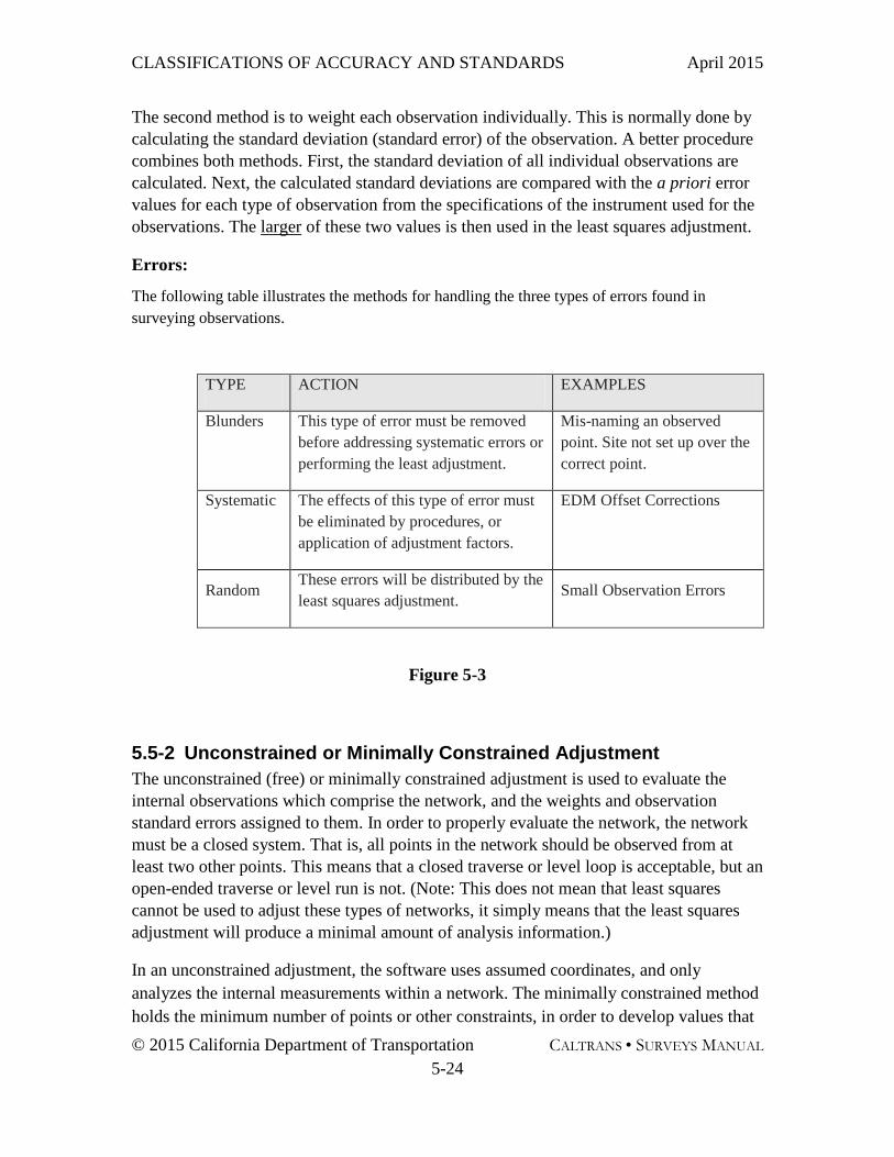
Errors:

The following table illustrates the methods for handling the three types of errors found in surveying observations.

TYPE ACTION EXAMPLES

Blunders This type of error must be removed before addressing systematic errors or performing the least adjustment.

Mis-naming an observed point. Site not set up over the correct point.

Systematic The effects of this type of error must be eliminated by procedures, or application of adjustment factors.

EDM Offset Corrections

Random These errors will be distributed by the least squares adjustment. Small Observation Errors

Figure 5-3

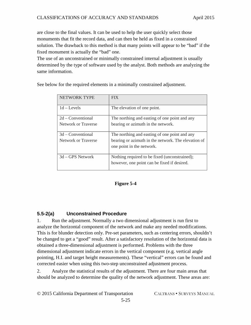
5.5-2 Unconstrained or Minimally Constrained Adjustment The unconstrained (free) or minimally constrained adjustment is used to evaluate the internal observations which comprise the network, and the weights and observation standard errors assigned to them. In order to properly evaluate the network, the network must be a closed system. That is, all points in the network should be observed from at least two other points. This means that a closed traverse or level loop is acceptable, but an open-ended traverse or level run is not. (Note: This does not mean that least squares cannot be used to adjust these types of networks, it simply means that the least squares adjustment will produce a minimal amount of analysis information.)

In an unconstrained adjustment, the software uses assumed coordinates, and only analyzes the internal measurements within a network. The minimally constrained method holds the minimum number of points or other constraints, in order to develop values that © 2015 California Department of Transportation CALTRANS • SURVEYS MANUAL

5-24


are close to the final values. It can be used to help the user quickly select those monuments that fit the record data, and can then be held as fixed in a constrained solution. The drawback to this method is that many points will appear to be “bad” if the fixed monument is actually the “bad” one. The use of an unconstrained or minimally constrained internal adjustment is usually determined by the type of software used by the analyst. Both methods are analyzing the same information. See below for the required elements in a minimally constrained adjustment.

NETWORK TYPE FIX

1d – Levels The elevation of one point.

2d – Conventional Network or Traverse

The northing and easting of one point and any bearing or azimuth in the network.

3d – Conventional Network or Traverse

The northing and easting of one point and any bearing or azimuth in the network. The elevation of one point in the network.

3d – GPS Network Nothing required to be fixed (unconstrained); however, one point can be fixed if desired.

Figure 5-4

5.5-2(a) Unconstrained Procedure 1. Run the adjustment. Normally a two dimensional adjustment is run first to analyze the horizontal component of the network and make any needed modifications. This is for blunder detection only. Pre-set parameters, such as centering errors, shouldn’t be changed to get a “good” result. After a satisfactory resolution of the horizontal data is obtained a three-dimensional adjustment is performed. Problems with the three dimensional adjustment indicate errors in the vertical component (e.g. vertical angle pointing, H.I. and target height measurements). These “vertical” errors can be found and corrected easier when using this two-step unconstrained adjustment process. 2. Analyze the statistical results of the adjustment. There are four main areas that should be analyzed to determine the quality of the network adjustment. These areas are:



• Standard Deviation of Unit Weight: (Also called Standard Error of Unit Weight, Error Total, Network Reference Factor, etc.) The closer this value is to 1.0, the better your network is weighted. The acceptable range is 0.8 to 1.2. In general, if all blunders have been removed, a value greater than 1.0 indicates that the observations are not as good as their assigned weights, while a value less than 1.0 indicates that the observations are better than their weights.

• Observation Residuals: Usually the adjustment output will include a listing which includes observations, residuals, standard errors, and a warning value or factor. The residual is the amount of adjustment applied to the observation to allow it to best fit the network. Many programs compare the residual to the observation standard error and then flag excessively large residuals. Some programs will flag observations when the residual is greater than three times the standard error. Large residuals may indicate blunders which were not previously identified and eliminated, or excessive noise in the GNSS data.

• Coordinate Standard Deviations and Error Ellipses: A network with a good Standard Deviation of Unit Weight and well weighted observations with no flagged residuals can still produce points with high standard deviations and large error ellipses (due to the effect, for instance, of network geometry). These values should be examined to determine if the point accuracies are high enough for their intended application.

• Relative Errors: These values are often shown as parts per million, and predict the amount of error which can be expected to be found between adjacent points in the network. However, values can also be shown as directional and distance errors in seconds and feet, respectively.

3. If necessary, make modifications as determined from the analysis of the adjustment statistical results. If justified, these modifications could include: (1) adding, deleting, or editing observations, (2) changing observation standard errors, and (3) modifying centering and standard H.I. errors.

• Adding, Deleting, or Editing Observations: At times, it is necessary to add observations to a network. If all other statistical indicators look good but some of the points have excessively large standard deviations, it is probably necessary to add additional observations to those points. Deleting observations may be required if they are proven to include blunders, that is, the observation simply does not fit the network. Sometimes, a good observation is listed using the wrong point names, in which case, editing the point names will remove the blunder.

• Changing Observation Standard Errors: Observation standard errors should not be changed without a good reason. The only justification for changing a standard error is special field conditions noted in the field notes. Normally, if an observation fits poorly and its standard error was calculated individually, it is a blunder. Justifying changing standard errors is more reasonable when the standard



errors were assigned on a group basis. However, if changes are made they should be made for the whole group, not for an individual observation.

• Modifying Centering and H.I. Standard Errors: Mistakes in assigning centering and H.I. errors is often misinterpreted as poor observation errors, especially if the standard errors were developed for observation groups. This problem is easier to detect when standard errors are developed individually. Always select the proper error for each instrument. A properly adjusted tribrach has a 2 mm centering error, while a standard GNSS rod usually has a 3 mm error.

4. Readjust the network. The unconstrained adjustment is an iterative process. It may be necessary to adjust and modify the network several times until an acceptable solution is determined. Once this has occurred, a report of the adjustment results should be stored for filing and labeled as being the unconstrained adjustment.

Note: Once the unconstrained/ minimally constrained adjustment has been accepted, no modifications of any type should be made to the network with the exception of fixing the coordinates of the control points.

5.5-3 Constrained Adjustment When performing control surveys, it is assumed that the existing control is superior to that which is performed later. The original control monuments are held fixed, and all adjustments are made to the new observations. Adjusting the network by holding it to fixed points is known as the constrained adjustment. This is the final step of a least squares adjustment, after the unconstrained/ minimally constrained adjustment.

5.5-3(a) Constrained Procedure 1. Fix the coordinates of the known control points. 2. Run the adjustment. 3. Analyze the effects of the fixed control on the network adjustment. This is done to determine the validity of the coordinates of the control points. The validity of the network observations was proven in the unconstrained adjustment phase. Depending on the quality of the reference system used to constrain the network, the Standard Deviation of Unit Weight of the final adjustment may not be close to 1.0 and many of the observation residuals may be flagged as being excessively large. This situation is acceptable if it has been determined that there are no blunders in the control. The surveyor in charge of the adjustment must decide if this degradation in quality is significant. If the survey network meets required accuracies, the adjustment is complete. If accuracy standards are not met, then modifications of the fixed points and readjustments may be appropriate. In cases where the coordinates of the control monuments are based on a superseded datum tag or epoch, and the accuracy standards for the adjustment can’t be met, it will be necessary to use a more recent datum tag in order to met specifications. © 2015 California Department of Transportation CALTRANS • SURVEYS MANUAL

5-27


4. Modify the fixed points as appropriate. There are two modification options available. First, check the fixed coordinates for errors transpositions, and mis-identifications. If required, edit the coordinates and readjust. If this is not the problem, then one or more of the control points is not in its published position. An analysis of the relationship of the control points can help determine which point or points are unacceptable.

A procedure, which can be used to analyze the control, is as follows:

• Calculate the inverse distance between the published positions of all the fixed control points.

• Calculate the inverse distance between the unconstrained positions of all the fixed control points.

• Calculate the difference between the published inverse distances and the unconstrained inverse distances.

• Using these differences and the published inverse distances calculate a ppm value for each inverse.

• Examine the ppm values. High ppm values indicate problems with the associated control. A control point which shows up in several of the inverses with high ppm values is probably not in its published position. Run the adjustment again with this point free.

• Alternatively, control points can be held free or fixed on a trial and error basis until the problem has been detected. Once a determination about the control is made the final adjustment is performed. After the final adjustment, a listing of the adjustment results should be printed out, labeled as the constrained adjustment, and filed along with a note about any control problems.

5. Re-adjust network, if necessary.

One commonly used least squares component is a statistical test called the Chi-Square test, used to give a pass/fail grade to the adjustment. This test compares the actual statistical results to the expected theoretical results (that is a standard deviation of unit weight of 1.0) given the number of degrees of freedom in the network. (Degrees of freedom equal the number of observations minus the number of unknowns in the network.) Obviously, it is desirable to pass this test; however, it is not an absolute requirement. If a network has a standard error of unit weight close to 1.0, no high observation residuals, and still does not pass the Chi-square test, the network should be accepted and the failure of the Chi-square test disregarded.



5.6 Compass Rule Adjustment A least squares adjustment is the preferred adjustment method, and can be used for GNSS, traverse, or level adjustments, whenever there are redundant measurements. For traverses without any redundant measurements, the compass rule adjustment is an acceptable method. The traverses can be either a closed traverse, which begins and ends on the same point; or a connecting traverse, which begins and finishes on two known points with an independent source of higher accuracy. The use of a closed loop is discouraged, as azimuth or scaling errors will not be detected. Open traverses, which begin on a known point, but end on an unknown, are not acceptable. Whenever possible, connecting traverses will not end just on a known point, but also with a turned angle along a known azimuth.

A compass adjustment will yield a closure ratio, which is the distance between the calculated and known closing coordinates, divided by the length of the traverse. The ratio is then used to determine the order of accuracy. A traverse can never have a higher order of accuracy than that of the initial control points. That is, a traverse between two azimuth pairs set with Second Order, Class II accuracy (1:20,000) cannot be considered a Second Order, Class I traverse, even with a closure ratio greater than 1:50,000.






5.7 Azimuth Pairs In order to provide control for total station surveys, intervisible monuments are set at each end of a project, to provide points with known coordinates and bearings. Additional pairs are spaced as needed within the project. These points are referred to as azimuth pairs. These pairs must meet requirements for both positional and relative accuracy. The accuracy of the azimuth of a baseline is a function of the length of the baseline and its relative error. To meet Caltrans standards, the minimum relative accuracy of a baseline between azimuth pairs is Second Order, Class II: either 1: 20,000, or ± 10" of arc.

The relative accuracy of the azimuth baseline in reciprocal form is 1: 𝑑𝑒

where: e is the linear error of the baseline as determined by the constrained adjustment. d is the distance between azimuth points.

You can use the ratio 𝑒𝑑

to find the maximum azimuth error, such that θ = arctan(𝑒𝑑).

This method assumes that the vector between azimuth points has been directly measured.

Example: A baseline has a distance of 521.50 meters, and the constrained adjustment has a linear error of ± 0.024 m.

1: 521.50.024

= 1: 21,729 θ = arctan (0.024521.5

) = ± 9 seconds

For network planning purposes, Table 3 of Geometric Geodetic Accuracy Standards and Specifications for Using GPS Relative Positioning Techniques (Reprinted 1989) uses the square root of the sum of the square of the two point 95% positional accuracies to determine the 95% error of the baseline, and then divide by the length of the line to determine the baseline azimuth (θ) accuracy.

Then the proposed accuracy of the baseline is 1: 𝑑𝑒

and 𝑒 = √𝑎2 + 𝑏2

Where: e is the estimated linear error of a baseline. a is the positional accuracy at the first station. b is the positional accuracy at the second station. d is the distance between azimuth points.





Example: If two points are 566 meters apart, and the planned network accuracy is 2 cm, then: 𝑒 = √0.022 + 0.022 = 0.0283

The estimated relative accuracy of the baseline length is 1: 𝑑𝑒 = 566

0.0283 = 1: 20,000

The relative accuracy of the baseline azimuth is θ = arctan (0.0283566

) = ± 10 seconds,

which is the Second Order, Class II standards of 1:20,000 or 10 seconds of arc. Using the above formulas for 95% network accuracies of 1 cm and 2 cm, the following table shows the minimum distances calculated to meet required azimuth accuracies.

Minimum Baseline Length

Order Relative Ratio

Azimuth Accuracy in Seconds

1 cm 95% Network Accuracy

2 cm 95% Network Accuracy

Second, Class I16 1: 50,000 ≤ 4" 707 m (2320 ft) 1414 m (4640 ft) Second, Class II 1: 20,000 ≤ 10" 283 m (928 ft) 566 m (1856 ft) Third 1: 10,000 ≤ 21" 141 m (464 ft) 283 m (928 ft)

Figure 5.5

This table is for planning purposes only. The linear error of the baseline and the distance between points will determine the final baseline accuracy. If the minimum distances in Figure 5.5 cannot be met in the field, more precise measurements may still allow a baseline to meet the required accuracy standards. Conversely, poor accuracy may result in a baseline that fails standards, even if the minimum distance requirements are met.

16 NGS Second Order, Class I is not generally required by Caltrans. If an azimuth pair does meet the Class I requirements, it should be documented as such in the Project Control Report (see Chapter 9). © 2015 California Department of Transportation CALTRANS • SURVEYS MANUAL

5-32


5.8 Monumentation For each level of accuracy, there is a corresponding requirement for the stability of the monument. Frost heave, moisture content, and stability of the surrounding soil all affect the lifespan of the published coordinates for each monument. If the requirements for monument stability aren’t met, a monument measured to a given order of accuracy should be published at a lower order that matches the monument stability. The monument descriptions below are the minimum requirements for each level. Monuments set to a higher level are acceptable for lower order surveys. Most monuments described in this Chapter are based on the following documents:

• NGS Bench Mark Reset Procedures, Curtis L. Smith, September 2010 (Referred to as “NGS 2010” in future references)

• USACE Manual EM 1110-1-1002, Survey Markers and Monumentation, March 2012 (Referred to as USACE Manual in future references)

• Caltrans Standard Plans 2010, Plan sheet A74. (Referred to as Standards Plans in future references

• Caltrans Surveys Manual, Chapter 10, Right of Way Surveys

5.8-1 Primary Control Monuments These monuments are set for primary control, usually to meet NGS standards (0.5 cm or better). There are only a few monument types that meet the strict requirements for horizontal and vertical accuracy. The first is a bronze/ brass disk set into a rock outcrop, large boulder, or massive concrete structure. The next is the NGS 3-D rod monument. Both types are described in NGS 2010. For vertical bench marks, a 12” dia. X 48” h concrete monument as shown in NGS 2010 is also acceptable. Existing NGS or USGS17 monuments may also be used as primary control points. All disks must be stamped with a unique identifier. Monuments without disks, such as NGS 3-D rods, must have the lid stamped. In addition to the stamping, a permanent witness post (metal or fiberglass) will be set nearby with the monument information affixed.

5.8-2 Project Control Monuments These monuments are required for all horizontal surveys with 1-cm or 2-cm network accuracies, or second order traverses. They are also required for all vertical project control surveys. Monuments are expected to remain stable for the life of a project, with a minimum service life of five years. They must be set at least one foot below frost depth, at a minimum of 30 inches total in depth. They must also remain stable when heavy equipment is operating nearby. Monument marking and witness post requirements are the same as above.

17 United States Geological Survey http://www.usgs.gov/ © 2015 California Department of Transportation CALTRANS • SURVEYS MANUAL

5-33

http://www.usgs.gov/


The following monuments are acceptable for project control:

• Primary Control Monuments as described above • Monument Types A, B, C and G as described in the USACE Manual, generalized

as: o Type A - Deep rod with 3-foot finned section o Type B - Stainless steel Deep rod with sleeve o Type C – Disk in rock or concrete o Type G – Cast-in- place concrete and disk

• Monument Types A, B, and D, or equivalent, as shown in the Caltrans Standard Plans, generalized as:

o Type A - Cast-in- place concrete monument and disk o Type B – Concrete monument and disk in well o Type D - Concrete monument and disk in well

• Manufactured control monuments, at least 30” long, such as: o Bernsten® Top Security Rod Monuments o Surv-Kap® Aluminum Rod Monuments o FENO® Survey Monuments

• Galvanized iron pipes with brass or aluminum disks. Pipes must be either 1” x 30”, or 2” x 24”, with the bottom of the pipes set a minimum of 30” below grade. Disks must be at least the same diameter as the pipe, and cemented or epoxied in place.

• For vertical control only, a 5/8” x 30” steel rebar with metal cap, with the bottom of the rebar set a minimum of 30” below grade.

5.8-3 Supplemental Monuments These monuments are used to densify control as needed within a project. They are typically temporary control set for engineering, right of way, or construction surveys. As supplemental control, they may not last the life of a project, and may be set using lesser quality materials. Typically they are 18” pipes or rebars, P.K. nails in paving, chiseled crosses in concrete, or similar materials. It’s up to the Party Chief to determine the expected life of the monument, and select the proper material accordingly. Plastic caps or plugs should only be used for horizontal points. Vertical points should have metal caps, or if made of steel or concrete, none at all. Permanent witness posts are not required.



5.9 Glossary of Terms18 The following are definitions of various terms used throughout the Geospatial Positioning Accuracy Standards. accuracy - closeness of an estimated (e.g., measured or computed) value to a standard or accepted [true] value of a particular quantity. (National Geodetic Survey, 1986). NOTE: Because the true value is not known, but only estimated, the accuracy of the measured quantity is also unknown. Therefore, accuracy of coordinate information can only be estimated (Geodetic Survey Division, 1996).

accuracy testing - process by which the accuracy of a data set may be checked.

check point - one of the points in the sample used to estimate the positional accuracy of the data set against an independent source of higher accuracy.

component accuracy - positional accuracy in each x, y, and z component.

confidence level - the probability that the true (population) value is within a range of given values. NOTE in the sense of this standard, the probability that errors are within a range of given values.

dataset - identifiable collection of related data.

datum - any quantity or set of such quantities that may serve as a basis for calculation of other quantities. (National Geodetic Survey, 1986)

elevation - height of a point with respect to a defined vertical datum.

ellipsoidal height - distance between a point on the Earth’s surface and the ellipsoidal surface, as measured along the perpendicular to the ellipsoid at the point and taken positive upward from the ellipsoid. NOTE also called geodetic height (National Geodetic Survey, 1986)

horizontal accuracy - positional accuracy of a dataset with respect to a horizontal datum. (Adapted from Subcommittee for Base Cartographic Data, 1998)

18 This glossary is copied from FGDC-STD-007.1-1998 (Part 1: Reporting Methodology) Appendix 1-A. © 2015 California Department of Transportation CALTRANS • SURVEYS MANUAL

5-35


horizontal error - magnitude of the displacement of a feature's recorded horizontal position in a dataset from its true or more accurate position, as measured radially and not resolved into x, y.

independent source of higher accuracy - data acquired independently of procedures to generate the dataset that is used to test the positional accuracy of a dataset. NOTE the independent source of higher accuracy shall be of the highest accuracy feasible and practicable to evaluate the accuracy of the data set.

local accuracy - The local accuracy of a control point is a value that represents the uncertainty in the coordinates of the control point relative to the coordinates of other directly connected, adjacent control points at the 95-percent confidence level. The reported local accuracy is an approximate average of the individual local accuracy values between this control point and other observed control points used to establish the coordinates of the control point. For Caltrans, surveys constrained to the passive project control are considered local accuracy.

network accuracy - The network accuracy of a control point is a value that represents the uncertainty in the coordinates of the control point with respect to the geodetic datum at the 95-percent confidence level. For NSRS network accuracy classification, the datum is considered to be best expressed by the geodetic values at the Continuously Operating Reference Stations (CORS) supported by NGS. By this definition, the local and network accuracy values at CORS sites are considered to be infinitesimal, i.e., to approach zero.

orthometric height - distance measured along the plumb line between the geoid and a point on the Earth’s surface, taken positive upward from the geoid. (Adapted from National Geodetic Survey, 1986).

positional accuracy - describes the accuracy of the position of features (adapted from ISO Standard 15046-13)

precision - in statistics, a measure of the tendency of a set of random numbers to cluster about a number determined by the set. (National Geodetic Survey, 1986). NOTE: If appropriate steps are taken to eliminate or correct for biases in positional data, precision measures may also be a useful means of representing accuracy. (Geodetic Survey Division, 1996).

root mean square error (RMSE) - square root of the mean of squared errors for a sample.



spatial data - information that identifies the geographic location and characteristics of natural or constructed features and boundaries of earth. This information may be derived from, among other things, remote sensing, mapping, and surveying technologies (Federal Geographic Data Committee, 1998). NOTE also known as geospatial data.

vertical accuracy - measure of the positional accuracy of a data set with respect to a specified vertical datum (adapted from Subcommittee for Base Cartographic Data, 1998).

vertical error - displacement of a feature's recorded elevation in a dataset from its true or more accurate elevation.

well-defined point - point that represents a feature for which the horizontal position is known to a high degree of accuracy and position with respect to the geodetic datum.






5.10 References Federal Geodetic Control Subcommittee, 1995, Specifications and Procedures to

Incorporate Electronic Digital/Bar-Code Leveling Systems, Version 4.1, 27 May 2004.

Federal Geographic Data Committee, Part 1, Reporting Methodology, Geospatial Positioning Accuracy Standards, FGDC-STD-0007.1-1998, Washington, D.C., 1998.

Federal Geographic Data Committee, Part 2, Standards for Geodetic Networks, Geospatial Positioning Accuracy Standards, FGDC-STD-007.2-1998: Washington, D.C., 1998.

Federal Geographic Data Committee, Part 3., National Standard for Spatial Data Accuracy, Geospatial Positioning Accuracy Standards, FGDC-STD-007.3-1998: Washington, D.C., 1998.

Federal Geographic Data Committee, Part 4: National Standards for Spatial Data Accuracy, Standards for Architecture, Engineering, Construction (A/E/C) and Facilities Management, FGDC-STD-007.4-2002, Washington, D.C., 2002

Geometric Geodetic Accuracy Standards and Specifications for Using GPS Relative Positioning Techniques (1989), Federal Geodetic Control Committee

Ghilani, C. D. and P. R. Wolf. 2014. Elementary Surveying: An Introduction to Geomatics. Prentice Hall Publishers, Upper Saddle River, NJ.

Guidelines for Establishing GPS-Derived Ellipsoid Heights (1997) NOAA Technical Manual NOS NGS-58, Zilkoski, et al.

Guidelines for Establishing GPS-Derived Orthometric Heights (2008) NOAA Technical Manual NOS NGS-59, Zilkoski, et al.

Bench Mark Reset Procedures, Smith, C.L., NGS, September 2010 Standards and Guidelines for Cadastral Surveys Using Global Positioning System

Methods (2001), USDA Forest Service, Dept. of the Interior, Bureau of Land Management

Standards and Specifications for Geodetic Control Networks (1984), Federal Geodetic Control Committee

TM 11-D1, Methods of Practice and Guidelines for Using Survey Grade GNSS to Establish Vertical Datum in the United States Geological Survey (2012), Rydlund, Paul H., and Densmore, Brenda K.

U.S. Army Corps of Engineers, Engineer Manual EM 1110-1-1002, Survey Markers and Monumentation, 1 March 2012








http://www.fgdc.gov/standards/standards_publications/





http://www.ngs.noaa.gov/PUBS_LIB/Benchmark_4_1_2011.pdf

http://www.fs.fed.us/database/gps/gpsusfs.htm

http://www.fs.fed.us/database/gps/gpsusfs.htm

http://www.ngs.noaa.gov/FGCS/tech_pub/1984-stds-specs-geodetic-control-networks.htm

http://pubs.usgs.gov/tm/11d1/


U.S. Army Corps of Engineers, Engineer Manual EM 1110-1-1003, NAVSTAR Global Positioning System Surveying , 28 February 2011

U.S. Army Corps of Engineers, Engineer Manual EM 1110-1-1005, Control and Topographic Surveying, 1 January 2007

User Guidelines for Single Base Real Time GNSS Positioning, Version 2.1(2011), William Henning, National Oceanic and Atmospheric Administration, National Geodetic Survey

USGS Global Positioning Application and Practice, United States Geological Survey (Website)


http://www.publications.usace.army.mil/Portals/76/Publications/EngineerManuals/EM_1110-1-1005.pdf

http://www.publications.usace.army.mil/Portals/76/Publications/EngineerManuals/EM_1110-1-1005.pdf

http://www.ngs.noaa.gov/PUBS_LIB/NGSRealTimeUserGuidelines.v2.1.pdf

http://water.usgs.gov/osw/gps/


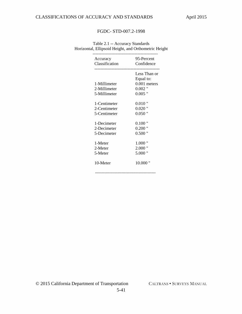
FGDC- STD-007.2-1998

Table 2.1 -- Accuracy Standards Horizontal, Ellipsoid Height, and Orthometric Height

--------------------------------------------- Accuracy 95-Percent Classification Confidence ---------------------------------------------

Less Than or Equal to:

1-Millimeter 0.001 meters 2-Millimeter 0.002 " 5-Millimeter 0.005 "

1-Centimeter 0.010 " 2-Centimeter 0.020 " 5-Centimeter 0.050 "

1-Decimeter 0.100 " 2-Decimeter 0.200 " 5-Decimeter 0.500 "

1-Meter 1.000 " 2-Meter 2.000 " 5-Meter 5.000 "

10-Meter 10.000 "

----------------------------------------------



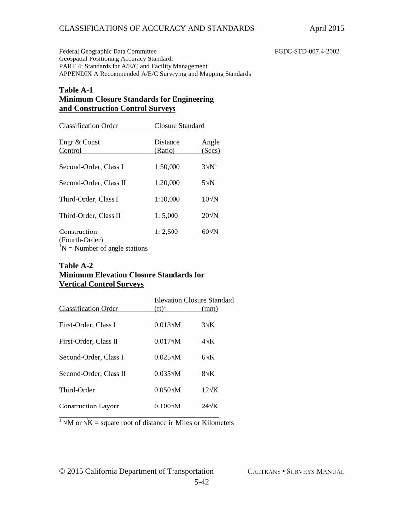
Federal Geographic Data Committee FGDC-STD-007.4-2002 Geospatial Positioning Accuracy Standards PART 4: Standards for A/E/C and Facility Management APPENDIX A Recommended A/E/C Surveying and Mapping Standards Table A-1 Minimum Closure Standards for Engineering and Construction Control Surveys Classification Order Closure Standard

Engr & Const Distance Angle Control (Ratio) (Secs)

Second-Order, Class I 1:50,000 3√N1

Second-Order, Class II 1:20,000 5√N

Third-Order, Class I 1:10,000 10√N

Third-Order, Class II 1: 5,000 20√N

Construction 1: 2,500 60√N (Fourth-Order)________________________________ 1N = Number of angle stations Table A-2 Minimum Elevation Closure Standards for Vertical Control Surveys

Elevation Closure Standard Classification Order (ft)1 (mm)

First-Order, Class I 0.013√M 3√K

First-Order, Class II 0.017√M 4√K

Second-Order, Class I 0.025√M 6√K

Second-Order, Class II 0.035√M 8√K

Third-Order 0.050√M 12√K

Construction Layout 0.100√M 24√K ____________________________________________ 1 √M or √K = square root of distance in Miles or Kilometers



Standards and Specifications for Geodetic Control Networks, Federal Geodetic Control Committee (1984)


Documents

CLASSIFICATIONS OF ACCURACY AND STANDARDS … · performed by Caltrans or others on all Caltrans-involved transportation improvement projects will be classified according to the standards