Classification of the Natural Gas Leak - Stanford …web.stanford.edu/class/cs231a/prev_projects_2016/report (5).pdf · Natural gas leak is a rising problem resulting in global warming

1

Abstract

Natural gas leak is a rising problem resulting in global

warming. Optical imaging technology is widely used for the leak detection, however, it lacks of the intelligence of knowing how big the leak is. The researcher comes up with a novel and interdisciplinary concept, making full use of the computer vision advances to automatically classify the natural gas leak. In this project, a support vector machine classifier with liner kernel, a support vector machine classifier with polynomial kernel and classification and regression trees (CART) are built to classify the natural gas leak happening in 20 meters, 30 meters away based on the extracted features after image enhancement and optical flow analysis. Sensitivity analysis were performed to examine the effect of feature selection, training and testing data size, noise threshold for optical flow calculation, number of frames which histogram of gradients (HOG) performs on. In conclusion, CART model with elastic net feature selection method is robust and has high accuracy when constructing a binary classification model for classifying the leak in different distances. Moreover, features can be HOG on enhanced images, HOG on orientation from optical flow and HOG on binary plume image. HOG can be calculated on the average of several frames in order to reduce the negative effect of the noise.

1. Introduction Natural gas leaks waste money, reduce energy

availability, and result in both local air quality and global climate impacts. The climate impacts of leaked gas are particularly important due to the high global warming potential of methane (a key component of natural gas).

Emissions of other hydrocarbons from natural gas also affect human health, because natural gas contains smog-forming and health-damaging organic compounds. In addition to environmental concerns, the economic impacts of gas leakage are clear: lost natural gas in the US costs nearly $2 billion per year at current prices.

Current EPA estimates suggest that about 1.5% of the natural gas produced in the US is lost in leaks, while recent studies suggest that potential emissions from the

gas system may be higher [1-3]. Currently many natural gas leak detection and repair (LDAR) technologies exist. These methods include manually operated flame ionization detectors and manually operated infrared (IR) video cameras for real-time optical gas imaging. EPA has recently released proposed regulations that codify the use of IR optical gas imaging as the standard leak detection technique (see Figure 1) [4]. The IR camera (owned by Brandt lab) measures IR radiation that that is strongly absorbed by methane and other natural gas components, so pollution plumes look black in the camera.

The researcher proposes an interdisciplinary project that expands upon EPA-approved IR imaging and will harness the potential for computer vision advances to allow for rapid automatic classification of methane leaks in order to solve the problem that now the infrared camera cannot tell the operator how big the leak is in the real time. There is a recent study conducted by my advisor Prof. Brandt illustrating the importance of classification: the top 5% of leaks in a given population can be expected to emit over 50% of total methane emissions [5]. In the future, this project will be further performed and join industry-standard imaging equipment to pollution dispersion models for rapid impact assessment for real-world leaks.

Fig. 1: Example methane plume visualized using IR camera I collected on Apr 18th.

2. Related Work There is few related work, which have been done to

classify the natural gas leak.

Classification of the Natural Gas Leak

Jingfan Wang

PhD student in Energy Resources Engineering [email protected]

2

Some researchers came up with great methodology to detect the leak, or the object, which preserves the unique shape as the plume, like smoke and wave.

Researchers from Providence Photonics, LLC, a U.S. based firm, achieves autonomous remote detection of plumes using computer vision and infrared optical gas imaging. The algorithm make use of the difference between a plume and the background in an IR image, discovers that the temporal change is because of the plume behavior, and reduce the possibility of detecting steam as plume [6].

Plume has distinct moving features than other objects. Green’s theorem explained the unique characteristic of plume motion, which is average upward motion above the source and divergence around the source [7]. Thus this will help examine whther the dynamic regions contain the plume.

DongKeun Kim, et al. performed connected component analysis to locate of interest (ROIs). Then the researchers decide whether the detected ROI is smoke by using the k- temporal information of its color and shape extracted from the ROI [8].

The researchers from UCLA vision lab discovered a novel definition of dynamic texture that is general and precise, and developed a new dynamic texture modeling method, which have already successfully used to detect fountain, ocean waves, fire and water [9].

For constructing feature descriptors used in computer vision and image processing, histogram of oriented gradients (HOG) is widely used for object detection [10].

For this project, the researcher successfully built up a binary classification model, resulting in a great contribution to the corresponding academic field, which few people have explored in.

3. Problem Statement and Technical Part In Apr 18th, 12 videos were collected in one field near

Sacramento. Each video stream has 240 * 320 resolution and was taken by FLIR researchIR software, which was connected to the IR camera when taking videos of the leak. More details about the collected videos can be found in Table 1. Six videos were taken either 20 meters or 30 meters away from the leak source. Leak size which unit is volume per time is an important metric to be used to compare different leaks of natural gas, not concentration. Totally there are 6 levels of leak size in all the collected videos. In this project, the researcher is trying to develop a accurate binary classification algorithm for classifying small leak and big leak, where the small leak is defined as any leak with leak size which is below 50 MSCF/day, however, the big leak is defined as any leak with leak size which is not less than 50 MSCF/day. The following are the steps of the technical solutions.

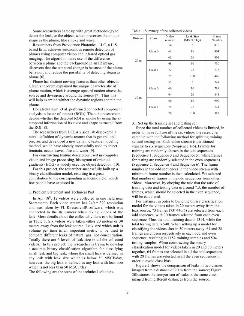
Table 1. Summary of the collected videos

3.1 Set up the training set and testing set Since the total number of collected videos is limited, in order to make full use of the six videos, the researcher came up with the following method for splitting training set and testing set. Each video stream is partitioned equally to six sequences (Sequence 1-6). Frames for training are randomly chosen in the odd sequences (Sequence 1, Sequence 3 and Sequence 5), while frames for testing are randomly selected in the even sequences (Sequence 2, Sequence 4 and Sequence 6). The frame number in the odd sequences in the video stream with minimum frame number is then calculated. We selected that number of frames in the odd sequences from other videos. Moreover, by obeying the rule that the ratio of training data and testing data is around 7:3, the number of frames, which should be selected in the even sequence, will be calculated.

For instance, in order to build the binary classification model for the videos taken in 20 meters away from the leak source, 73 frames (73≈440/6) are selected from each odd sequence, with 30 frames selected from each even sequence. Thus the total training data is 1314, while the total testing data is 540. When setting up a model for classifying the videos shot in 30 meters away, 64 and 28 frames are chosen respectively in each odd and even sequence, resulting in 1152 training samples and 504 testing samples. When constructing the binary classification model for videos taken in 20 and 30 meters together, 64 frames are selected in all the odd sequences with 28 frames are selected in all the even sequences in order to avoid class bias.

Figure 2 shows the comparison of leaks in two classes imaged from a distance of 20 m from the source; Figure 3illustrates the comparison of leaks in the same class imaged from different distances from the source.

Distance Class Video number

Leak Size (MSCF/Day)

Frame Number

20 m

Class 0

54 5 816

61 10 904

63 20 801

Class 1

68 50 730

72 75 738

79 100 440

30 m

Class 0

55 5 749

60 10 789

64 20 843

Class 1

69 50 999

71 75 721

78 100 385

3

Fig 2. (a) A single frame of a controlled leak corresponding to 20 MSCF/day (class 0) imaged from a distance of 20 m from the source (Video No. 63). (b) A single frame of a controlled leak corresponding to 100 MSCF/day (class 1) imaged from a distance of 20 m from the source (Video No. 79).

Fig 3. (a) A single frame of a controlled leak corresponding to 20 MSCF/day (class 0) imaged from a distance of 20 m from the source (Video No. 63). (b) A single frame of a controlled leak corresponding to 20 MSCF/day (class 0) imaged from a distance of 30 m from the source (Video No. 64).

3.2 Preprocess the training and testing data

Instead of preprocessing all the collected videos, it saves a great deal of time to just preprocess the training and testing data. By looking at the collected data on Apr 18th, the natural gas leak sometimes cannot be easily differentiated from the background. Thus before developing the classification algorithm, contrast enhancement should be performed. The frame is initially filtered using a ‘top-hat’ transform with a disk structural element of size 10. Top-hat filtering is used to correct uneven background illumination when the background is darker than the foreground [11]. The contrast between the background and the plume is further enhanced using adaptive histogram equalization. By effective spreading out the most frequent intensity values, this method works well when the backgrounds and foregrounds are both bright or both dark [6]. This technique works better than simple histogram equalization in terms of preserving the size and shape of the plume as shown in the videos. Moreover, the researcher also removed the pipe out of the every frame in order to have a better view of just the plume. An example illustrating the preprocessed image is shown in Fig 4.

Fig. 4: Example of the preprocessed image.

3.3 Extraction of features

Extraction of features of training and testing data is performed based on the preprocessed frames.

The natural gas leak can be detected via its unique motion. Optical flow can help to select the dynamic regions of the plume and eliminate the stationary areas, and accurately measure the motions of the plume. Specifically, Pyramidal Lucas-Kanade optical flow method is implemented [6]. The optical flow of the plume, the magnitude and direction of plume pixels, is computed using an appropriate noise threshold that captures the shape and size of the plume. The greater the noise threshold is, the less movement affects the optical flow calculation, however, the less the noise threshold is, the more motion can be captured and calculated. The following way shows the steps for choosing the noise threshold in the analysis. Firstly the researcher set a relatively large threshold. Secondly the value is decreasing until the arrows just can capture the shape of the plume. The resultant image is converted to a binary image by counting pixels with non-zero flow as part of the plume to obtain approximate pixel coverage values. The original frame, optical flow data in the plume and the extracted plume coverage are shown in Fig. 5. From Fig 5, it is clear that the shape of the plume in the binary image resulted from the optical flow analysis is almost the same as that in the raw image.

4

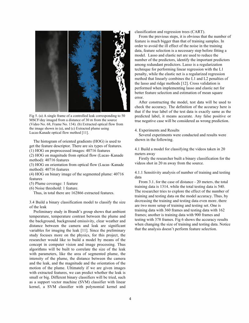
Fig 5. (a) A single frame of a controlled leak corresponding to 50 MSCF/day imaged from a distance of 30 m from the source (Video No. 68, Frame No. 134). (b) Extracted optical flow from the image shown in (a), and (c) Extracted plume using Lucas-Kanade optical flow method [11].

The histogram of oriented gradients (HOG) is used to get the feature descriptor. There are six types of features. (1) HOG on preprocessed images: 40716 features (2) HOG on magnitude from optical flow (Lucas–Kanade method): 40716 features (3) HOG on orientation from optical flow (Lucas–Kanade method): 40716 features (4) HOG on binary image of the segmented plume: 40716 features (5) Plume coverage: 1 feature (6) Noise threshold: 1 feature.

Thus, in total there are 162866 extracted features. 3.4 Build a binary classification model to classify the size of the leak

Preliminary study in Brandt’s group shows that ambient temperature, temperature contrast between the plume and the background, background emissivity, clear weather and distance between the camera and leak are significant variables for imaging the leak [11]. Since the preliminary study focuses more on the physics, for this project, the researcher would like to build a model by means of the concept in computer vision and image processing. Thus algorithms will be built to correlate the size of the leak with parameters, like the area of segmented plume, the intensity of the plume, the distance between the camera and the leak, and the magnitude and the orientation of the motion of the plume. Ultimately if we are given images with extracted features, we can predict whether the leak is small or big. Different binary classifiers will be tried, such as a support vector machine (SVM) classifier with linear kernel, a SVM classifier with polynomial kernel and

classification and regression trees (CART). From the previous steps, it is obvious that the number of

feature is much bigger than that of training samples. In order to avoid the ill effect of the noise in the training data, feature selection is a necessary step before fitting a model. Lasso and elastic net are used to reduce the number of the predictors, identify the important predictors among redundant predictors. Lasso is a regularization technique for performing linear regression with the L1 penalty, while the elastic net is a regularized regression method that linearly combines the L1 and L2 penalties of the lasso and ridge methods [12]. Cross validation is performed when implementing lasso and elastic net for better feature selection and estimation of mean square error.

After constructing the model, test data will be used to check the accuracy. The definition of the accuracy here is that if the true label of the test data is exactly same as the predicted label, it means accurate. Any false positive or true negative case will be considered as wrong prediction.

4. Experiments and Results

Several experiments were conducted and results were shown in the following. 4.1 Build a model for classifying the videos taken in 20 meters away

Firstly the researcher built a binary classification for the videos shot in 20 m away from the source. 4.1.1 Sensitivity analysis of number of training and testing data

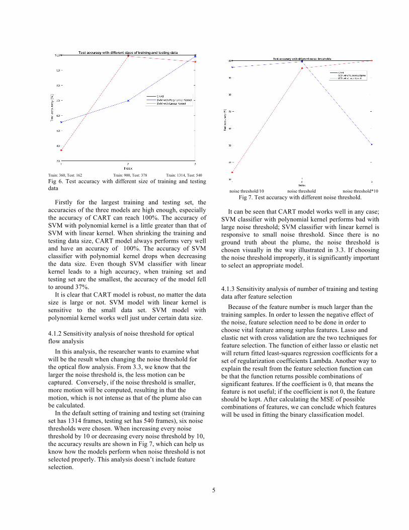
From 3.1, for the case of distance - 20 meters, the total training data is 1314, while the total testing data is 540. The researcher tries to explore the effect of the number of training and testing data on the model accuracy. Thus, by decreasing the training and testing data even more, there are two more setup of training and testing set. One is training data with 360 frames and testing data with 162 frames; another is training data with 900 frames and testing with 378 frames. Fig 6 shows the accuracy results when changing the size of training and testing data. Notice that the analysis doesn’t perform feature selection.

5

Train: 360, Test: 162 Train: 900, Test: 378 Train: 1314, Test: 540 Fig 6. Test accuracy with different size of training and testing data

Firstly for the largest training and testing set, the accuracies of the three models are high enough, especially the accuracy of CART can reach 100%. The accuracy of SVM with polynomial kernel is a little greater than that of SVM with linear kernel. When shrinking the training and testing data size, CART model always performs very well and have an accuracy of 100%. The accuracy of SVM classifier with polynomial kernel drops when decreasing the data size. Even though SVM classifier with linear kernel leads to a high accuracy, when training set and testing set are the smallest, the accuracy of the model fell to around 37%.

It is clear that CART model is robust, no matter the data size is large or not. SVM model with linear kernel is sensitive to the small data set. SVM model with polynomial kernel works well just under certain data size.

4.1.2 Sensitivity analysis of noise threshold for optical flow analysis

In this analysis, the researcher wants to examine what will be the result when changing the noise threshold for the optical flow analysis. From 3.3, we know that the larger the noise threshold is, the less motion can be captured. Conversely, if the noise threshold is smaller, more motion will be computed, resulting in that the motion, which is not intense as that of the plume also can be calculated.

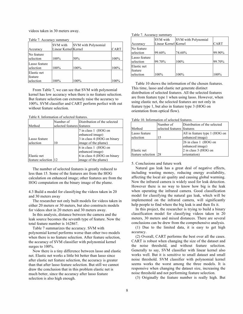
In the default setting of training and testing set (training set has 1314 frames, testing set has 540 frames), six noise thresholds were chosen. When increasing every noise threshold by 10 or decreasing every noise threshold by 10, the accuracy results are shown in Fig 7, which can help us know how the models perform when noise threshold is not selected properly. This analysis doesn’t include feature selection.

noise threshold/10 noise threshold noise threshold*10

Fig 7. Test accuracy with different noise threshold.

It can be seen that CART model works well in any case; SVM classifier with polynomial kernel performs bad with large noise threshold; SVM classifier with linear kernel is responsive to small noise threshold. Since there is no ground truth about the plume, the noise threshold is chosen visually in the way illustrated in 3.3. If choosing the noise threshold improperly, it is significantly important to select an appropriate model.

4.1.3 Sensitivity analysis of number of training and testing data after feature selection

Because of the feature number is much larger than the training samples. In order to lessen the negative effect of the noise, feature selection need to be done in order to choose vital feature among surplus features. Lasso and elastic net with cross validation are the two techniques for feature selection. The function of either lasso or elastic net will return fitted least-squares regression coefficients for a set of regularization coefficients Lambda. Another way to explain the result from the feature selection function can be that the function returns possible combinations of significant features. If the coefficient is 0, that means the feature is not useful; if the coefficient is not 0, the feature should be kept. After calculating the MSE of possible combinations of features, we can conclude which features will be used in fitting the binary classification model.

6

Fig 8.Test MSE with different combination of features after running Lasso function on training data with 1314 frames and testing data with 540 frames.

From Fig 8, we can see that the combination of features based on the 37th Lambda value will result in the lowest MSE. Thus, this combination of features can be further used as predictors when building the model. Table 2 summarizes the accuracy of different models after feature selection.

Table 2. Model accuracy after feature selection

From the table above, we found that after feature selection, the accuracy improves a lot. Previously the accuracy results of SVM with linear kernel and polynomial kernel for any case are not 100%. Especially SVM classifier with polynomial kernel performs extremely bad when the training set has 900 frames and the testing set has 378 frames. Now the accuracy results all increase to 100%. Feature selection chooses the most

important features and reduces the ill influence of the noise. In this analysis, there is no difference between lasso and elastic net.

It is very interesting to examine what the selected features are and which feature type the selected features belong to. If we found that some type of feature is not selected, in the future, we may not include that type of feature when fitting the model. Table 3 summarizes the information of the selected features. Table 3. Information of the selected features.

Case Method

Number of selected features

Distribution of the selected features

Train: 900, Test: 378

Lasso Feature Selection 17

All in feature type 1 (HOG on enhanced image)

Elastic net feature selection 19


Train:1314, Test: 540

Lasso feature selection 14




Originally there are 162866 features. After feature selection, there are only less than 25 features. Moreover all the selected features are from feature type 1, which is HOG on the enhanced image.

In the future, if the data is still limited, we can firstly try to only use HOG on enhanced images as predictors. The accuracy could be good enough.

One advantage of feature selection is that fitting the classification model by means of the selected features greatly saves the calculation time a lot.

4.1.4 Sensitivity analysis of noise threshold for optical flow analysis after feature selection

From Fig 5, it is concluded that SVM classifier with polynomial kernel is sensitive to large noise threshold, while SVM classifier with linear kernel is sensitive to small noise threshold. But after implementing feature selection, from Table 4, it is clear that the accuracy is significantly improved. Now it seems neither model is responsive to small or large noise threshold. Feature selection can help avoid the negative effect of not choosing noise threshold properly.

Accuracy

SVM with Linear Kernel

SVM with Polynomial Kernel CART


No feature selection 99.21% 69.84% 100% Lasso feature selection 100% 100% 100% Elastic net feature selection 100% 100% 100%


No feature selection 95.56% 99% 100% Lasso feature selection 100% 100% 100% Elastic net feature selection 100% 100% 100%

7

Table 4. Sensitivity analysis of noise threshold for optical flow analysis after feature selection

Train: 1314, Test: 540 Accuracy

SVM with Linear Kernel


Noise threshold/10

No feature selection 34.07% 96.11% 100% Lasso feature selection 100% 100% 100% Elastic net feature selection 99% 100% 100%

Noise threshold*10

No feature selection 100% 50.56% 100% Lasso feature selection 100% 100% 100% Elastic net feature selection 100% 100% 100%

The analysis of the selected features can be found in

Table 5. Firstly, feature selection reduces the feature number to less than 35. When the noise threshold is small, the selected features after either lasso or elastic net are not only from feature type 1 (HOG on enhanced image), but also from feature type 2 (HOG on magnitude from optical flow) and feature type 4 (HOG on binary image of the plume). However, when the noise threshold is big, all the chosen features are from feature type 1. The result is also illustrative for future modeling. Features from HOG on enhanced image can be fed in the model when the noise threshold is large. If the noise threshold is small, more features from other class, like class 2 and 4, should also be calculated and included. Table 5. Summary of selected features

Case: Train: 1314, Test: 540 Method

Number of selected features


Noise threshold/10


4 in class 1 (HOG on enhanced image) 3 in class 2 (HOG on magnitude from optical flow ) 9 in class 4 (HOG on binary image of the plume)


10 in class 1 (HOG on enhanced image) 10 in class 2 (HOG on magnitude from optical flow ) 12 in class 4 (HOG on binary image of the plume)

Noise threshold*10

Lasso feature selection

14 All in feature type 1 (HOG on enhanced image)



4.1.5 Sensitivity analysis of number of frames which HOG performs on Previously when extracting features from training and testing data, HOG was calculated on every frame. There is a thought came up with Prof. Savarese. If HOG was performed on the average of several consecutive frames and then the resultant features are fed into the model, how does the accuracy change? Because the accuracy results of three models for the default dataset (Train: 1314, Test: 540) are high enough, and feature selection also results in great accuracy, in order to see the change of the accuracy, the sensitivity analysis of number of frames which HOG performs on was conducted with the dataset including 900 training frames and 378 testing frames and without feature selection. In the analysis, HOG is computed on the average of every five frames. Table 6 shows the accuracy comparison with the change of the number of frames HOG works on. Table 6. Accuracy comparison when changing the number of frames HOG works on

Accuracy SVM with Linear Kernel


HOG on every frame 99.21% 69.84% 100% HOG on the average of every five frames 95.83% 95.83% 100%

From Table 6, it is clear that when the number of frames HOG performs on increases and changes to five, the accuracy of SVM with polynomial kernel greatly increases. Even though the accuracy of the SVM with linear kernel decreases a little bit, but still the accuracy is high enough for a binary classification model. If HOG works on more frames, not only one frame, it can significantly reduce the bad effect of some noise, like a bird flying over, or a man walking by in some frames. Notice that this is the only section talking about changing number of frames HOG works on. In all other analysis, HOG feature is calculated on every frame. 4.2 Build a model for classifying the videos taken in 30 meters away

Similarly, a binary classification can be built on the

8

videos taken in 30 meters away. Table 7. Accuracy summary



No feature selection 100% 50% 100% Lasso feature selection 100% 100% 100% Elastic net feature selection 100% 100% 100%

From Table 7, we can see that SVM with polynomial kernel has low accuracy when there is no feature selection. But feature selection can extremely raise the accuracy to 100%. SVM classifier and CART perform perfect with out without feature selection. Table 8. Information of selected features.

Method Number of selected features



7 in class 1 (HOG on enhanced image) 3 in class 4 (HOG on binary image of the plume)


6 in class 1 (HOG on enhanced image) 6 in class 4 (HOG on binary image of the plume)

The number of selected features is greatly reduced to

less than 15. Some of the features are from the HOG calculation on enhanced image; other features are from the HOG computation on the binary image of the plume. 4.3 Build a model for classifying the videos taken in 20 and 30 meters away

The researcher not only built models for videos taken in either 20 meters or 30 meters, but also constructs models for videos shot in 20 meters and 30 meters away. In this analysis, distance between the camera and the leak source becomes the seventh type of feature. Now the total feature number is 162867. Table 7 summarizes the accuracy. SVM with polynomial kernel performs worse than other two models when there is no feature selection. After feature selection, the accuracy of SVM classifier with polynomial kernel surges to 100%. Now there is a tiny difference between lasso and elastic net. Elastic net works a little bit better than lasso since after elastic net feature selection, the accuracy is greater than that after lasso feature selection. But still we cannot draw the conclusion that in this problem elastic net is much better, since the accuracy after lasso feature selection is also high enough.

Table 7. Accuracy summary



No feature selection 99.60% 74.60% 99.90% Lasso feature selection 99.70% 100% 99.70% Elastic net feature selection 100% 100% 100%

Table 10 shows the information of the chosen features. This time, lasso and elastic net generate distinct distribution of selected features. All the selected features are from feature type 1 when using lasso. However, when using elastic net, the selected features are not only in feature type 1, but also in feature type 3 (HOG on orientation from optical flow). Table 10. Information of selected features.

Method Number of selected features





26 in class 1 (HOG on enhanced image) 2 in class 3 (HOG on orientation)

5. Conclusions and future work

Natural gas leak has a great deal of negative effects, including wasting money, reducing energy availability, affecting the local air quality and causing global warming. Now the infrared camera is widely used for leak detection. However there is no way to know how big is the leak when operating the infrared camera. Good classification model for classifying the natural gas leak, which will be implemented on the infrared camera, will significantly help people to find where the big leak is and then fix it.

In this project, the researcher is trying to build a binary classification model for classifying videos taken in 20 meters, 30 meters and mixed distances. There are several conclusions can be drew from the comprehensive analysis.

(1) Due to the limited data, it is easy to get high accuracy.

(2) Overall, CART performs the best over all the cases. CART is robust when changing the size of the dataset and the noise threshold, and without feature selection. Generally to say, SVM classifier with linear kernel also works well. But it is sensitive to small dataset and small noise threshold. SVM classifier with polynomial kernel seems works the worst among the three models. It is responsive when changing the dataset size, increasing the noise threshold and not performing feature selection.

(3) Originally the feature number is really high. But

9

feature selection can significantly reduce the feature number, choose the meaningful features among redundant data for fitting the model and remove noise. Lasso and elastic net are the techniques for feature selection in the analysis. It works out that these two methods perform well, greatly reducing the feature number and increasing the accuracy. It seems elastic net works a little bit better than lasso. But further analysis should be conducted in order to find which is the most suitable for this kind of analysis.

(4) After the feature selection, the feature number is extremely reduced. When building up a model based on the selected features, the calculation time reduces a lot. It is helpful to implement in the infrared camera in the future for analyzing the leak in the real time.

(5) The selected features are always from the HOG calculation on the enhanced images. Thus if people just calculate HOG on the enhanced images and use the calculation results as features, the model could result in high accuracy. Other features like HOG on orientation from optical flow and HOG on binary image showing the plume are also helpful for fitting the model.

(6) Increasing the number of frames HOG is calculated on can greatly shrink the negative effect of noise, and increase the accuracy.

(7) In general, if building up a binary classification model for classifying the leak in different distances, CART model with elastic net feature selection method can be chosen. Moreover, features can be HOG on enhanced images, HOG on orientation from optical flow and HOG on binary plume image. HOG can be calculated on the average of several frames.

Since this project is a part of my PhD topic, in the future I will definitely go on working on this project. There are several directions I will work on.

(1) Collect more data of natural gas leak. The videos will taken in different distances, camera views, and atmospheric conditions.

(2) Develop more robust detection algorithm of the plume (3) Instead of conducting a binary classification problem, a regression model will be built in order to predict the leak size. (4) Try to use CNN and RNN. Code https://www.dropbox.com/sh/9jy2pjq8bfhwknw/AABFPjPbSNynWhQ1UaB-EDFNa?dl=0 Acknowledgement Recently I was awarded the Stanford Interdisciplinary Graduate Fellowship since I am working on automatic detection and quantification of the natural gas leak as my PhD topic. This project is a part of my PhD topic. Since this quarter is my first quarter in PhD life, actually this

class project is the fundamental brick for my future PhD research. Even though this class is my first CS class with letter grade, I think I did relatively good job on the project. Thus I feel happy that I made progress on the PhD project. I almost went to every office hour of Prof. Savarese and my project advisor, Kenji Hata. Thank you so much for your kind support and patience. I should also say thank you to other TAs, since they really did an extremely good job. Moreover, recently I submitted a paper which is 11th in the references, talking about whether the optical gas imaging is effective for methane detection. In the paper, I used the results of optical flow analysis and counted the plume coverage based on the binary image of the plume. The plume coverage from optical flow analysis is close to the result from the simulation we developed in our lab. Thus, this class project helps me a lot. Thank you so much!

References [1] Brandt, A. R., Heath, et al. (2014). Methane leaks from North American natural gas systems. Science, 343(6172), 733-735. [2] Miller, S. M., Wofsy, S. C., et al. (2013). Anthropogenic emissions of methane in the United States. Proceedings of the National Academy of Sciences,110(50), 20018-20022. [3] Zavala-Araiza, D., Lyon, D. R., Alvarez, R. A., Davis, K. J., Harriss, R., Herndon, S. C., ... & Marchese, A. J. (2015). Reconciling divergent estimates of oil and gas methane emissions. Proceedings of the National Academy of Sciences, 112(51), 15597-15602. [4] Environmental Protection Agency, Oil and Natural Gas Sector: Emissions Standards for New and Modified Sources, Federal Register, 40 CFR Part 60, 21023 (2015). [5] Brandt, A. R., et al. Super-Emitting natural gas leaks: implications for solving the methane challenge. (In review) [6] H. M., Morris, J. M., Ruan, Y., & Zeng, Y. (2013, September). Remote Gas Detection System Using Infrared Camera Technology and Sophisticated Gas Plume Detection Computer Algorithm. In SPE Annual Technical Conference and Exhibition. Society of Petroleum Engineers. [7] Altun, M., & Celenk, M. (2013, January). Smoke Detection in Video Surveillance Using Optical Flow and Green's Theorem. In Proceedings of the International Conference on Image Processing, Computer Vision, and Pattern Recognition (IPCV) (p. 1). The Steering Committee of The World Congress in Computer Science, Computer Engineering and Applied Computing (WorldComp) [8] Kim, D., & Wang, Y. F. (2009, March). Smoke detection in video. InComputer Science and Information Engineering, 2009 WRI World Congress on (Vol. 5, pp. 759-763). IEEE. [9] Gianfranco Doretto / Research / Project. Dynamic Texture Modeling. URL: http://vision.ucla.edu/~doretto/projects/dynamic-textures.html#results [10] Dalal, N. and B. Triggs. "Histograms of Oriented Gradients for Human Detection", IEEE Computer Society Conference on Computer Vision and Pattern Recognition, Vol. 1 (June 2005), pp. 886–893.

10

[11] Ravikumar, P.A., Wang J, Brandt, A. R. Are Optical Gas Imaging Technologies E ective For Methane Leak Detection? . (In review) [12] Lasso. Mathworks. . URL: http://www.mathworks.com/help/stats/lasso.html

Documents

Classification of the Natural Gas Leak - Stanford …web.stanford.edu/class/cs231a/prev_projects_2016/report (5).pdf · Natural gas leak is a rising problem resulting in global warming