1/24

Classification of Classification of Random ProcessesRandom Processes

2/24

There are several different ways to Classify Random Processes:

1) Type of Time Index* Continuous–Time: x(t) t∈(-∞,∞)* Discrete-Time: x[k] k∈ integers

2) Type of Values* Continuous-Value: x(t) takes values over an

interval, possibly (-∞,∞)* Discrete-Value: x(t) takes values from a

discrete set (e.g. the integers)

3/24

3) Type of Time Dependence of PDFs

When discussing a RP’s PDF above we have allowed for the most general time dependence. However, in practice many RP’s have Restricted Time-Dependence (e.g., WSS).

Ergodic

All Random Processes

Wide Sense Stationary (WSS)

Strictly Stationary (SS)

Ergodic ⊂ SS ⊂ WSS ⊂ All RPs

“Nonstationary RP” = One that is not WSS

4/24

(Strictly) Stationary ProcessesRough Definition : A RP whose entire statistical

characterization doesn’t change with time

)(),...,(,;,...(

),...,,;,...,(

12112,1

2121

nn

nn

tttxxxp

tttxxxp

Δ+Δ+=Depends on t1, Δ2,…Δn

Absolute Time Relative Times

To Get A More Precise Definition….First consider the nth order PDF and re-write it as :

5/24

(Strictly) Stationary ProcessesPrecise Definition : A Process is (strictly) stationary if, for all orders of n,

p(x1,x2,…,xn; t1, t1+ Δ2,…,t1+Δn)

does not depend on t1 but only on Δ2,…Δni.e. it depends only on relative time between points

NOTE 1: Since the 1st Order PDF p(x1;t1) does not depend on any relative time, a SS process must have a time-independent 1st Order PDF:

p(x1;t1) =p(x1)

6/24

Time-Invariant 1st Order PDF

0100

200300

400

-50

0

500

0.01

0.02

0.03

0.04

k (time index) x (value)

PDF: p(x;k) = p(x)

7/24

Stationary ProcessesThus a Stationary process must have:

Constant Mean :

Constant Variance :

∫∞

∞−

==⋅ constant);( xmdxtxpx= p(x) for stationary

process

constant )()(

);())((

2 ==⋅−=

⋅−

∫

∫∞

∞−

∞

∞−

xx

x

dxxpmx

dxtxptmx

σ

<<These are “necessary” but not “sufficient” conditions for SS>>

8/24

Stationary ProcessNote 2 : A Stationary process’s 2nd Order PDF depends only on the difference t = t2 - t1: P(x1,x2; τ)

Thus a stationary process must have : Autocorrelation Function that depends only on τ = t2 - t1

Rx (t1,t2) = Rx(t1, t1 + τ)= E{ x(t1) x(t1 + τ)}

Does not depend on t1 if x(t) is stationary

)(

);,( 212112

τ

τ

x

x

R

dxdxxxpxx

=

⋅⋅= ∫ ∫∞

∞−

∞

∞−

9/24

Stationary ProcessNote : As a 2-D function, Rx(t1 – t2) for a stationary

process looks like this: (t2 – t1) = +1 ……….. (τ = 1)

(t2 - t1) = 0 ……. (τ = 0)(t2 - t1) = -1 …. (τ =-1)

Rx(t1- t2) is constanton each of these lines Only a Function of τ = t2 – t1

t1

t2τ

10/24

An ACF That Depends Only On t2 – t1

-10 -5 0 5 10

-10-5

05

100

0.2

0.4

0.6

0.8

1

t1t2

Rx(t2 - t1)

11/24

Stationary Process

Now, A stationary process must have these 3 properties BUT BUT … must also have the similar properties for all the higher Order PDF’s!

That’s a lot to ask of a process in practice!

In Practice we “lower our standards” and we are mostly interested in so-called “wide-sense stationary” (WSS) processes.

12/24

Wide-Sense Stationary

A Process X(t) is said to be wide-sense stationary (WSS) if both of the following conditions are satisfied:

1) E{X(t)} = Constant

2) RX(t1, t2) = RX(τ)

ACF depends only on a time Difference

Constant Mean

Where τ = t1- t2

13/24

Wide-Sense StationaryNOTE : A WSS Process has a constant Variance

Proof By Definition :

22

22

22

)}({2)}({

})(2)({

}))({(

xtxExtxE

xtxxtxE

xtxEx

+−=

+−=

−=σ

RX(0)

2x−

x

14/24

Wide-sense Stationary

22 )0( xR xx −=σTrue for Stationary or WSS process

Passing Comment:Alot of the analysis DSP engineers do centers around Specifying an Appropriate Model for a random signal expected to be encountered and Determining if the Model is WSS.

Thus we have proved:

15/24

Example of RP ModelX(t) = A COS ( ωC t + θ)

Good model for a received sinusoid since we have no idea what Phase the transmitter used

…thus phase could be anything ⇒ each value is equally likely

So… Model θ as a RV uniformly distributed between 0 & 2π

Not Random Random Variable

16/24

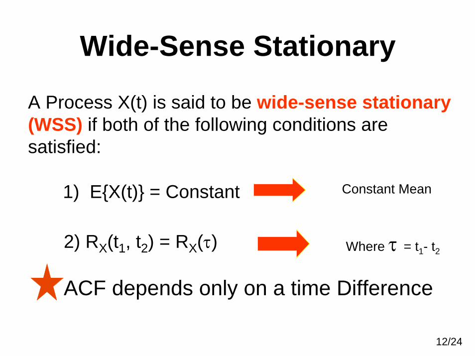
Example of RP Model (cont.)

PDF of θ :

Q : What does this Model Say ?

p(θ)

θ

Needed to give a unit area for PDF

0 2π

π21

⎪⎩

⎪⎨

⎧ ≤≤=

otherwise,0

20,21

)(πθ

πθp

17/24

Example of RP Model (cont.)

A : Transmitter (Tx) randomly “picks” a single phase value from 0 to 2π and generates a realization

A COS (ωCt + θ)

Each time the Tx is turned on we randomly get a new phase

Note : Once picked, θ doesn’tchange with time

18/24

Example of RP Model (cont.)Q: Which of our two “view points” is easier to think of for this example?

1. Sequence of RVs???2. Collection of Waveforms & Pick One???

A : Clearly it is easier to view this random processas a collection of waveforms from which you randomly pick one

Remember!!! – Both Views are Still Correct

19/24

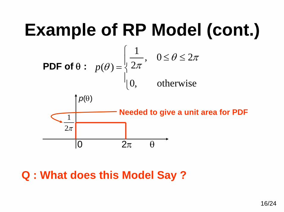
Example of RP Model (cont.)Here are 4 realizations (sample functions) of the ensemble of this process

Each one has a different Phase

Which signal you get is randomly chosen according to the PDF of Phase

A

-A

t

A

-A

t

A

-A

t

A

-A

t

20/24

Example of RP Model (cont.)Looking at any one sample function doesn’t give the appearance of being a random process !

BUT IT IS RANDOM! You don’t know ahead of time which you were going to get.In this case, randomness is best viewed as “notknowing which of the infinite possible sample functions you will get”

So… now we have a model for a practical signal scenario. Now What???

Do analysis to characterize the model !!!!

21/24

Example of RP Model (cont.)Task : Find the mean and the ACF of this process

& Ask: Is It WSS?Mean = E{x(t)} = E{A cos (ωct + θ ) }

= A E{ cos(ωct + θ )}

∫

∫

+=

+=

π

π

θθωπ

θπ

θω

2

0

2

0

)cos(2

21)cos(

dtA

dtA

c

c

Integrating over one fullcycle for each fixed t value:

= 0

So Far We’ve Shown:MEAN = CONSTANT!

Exp. Val. of Function of a RVIf Z is a RV w/ PDF P(z)

then W = f(Z) is a new RV w/

∫== dzzPzfZfEWE z )()()}({}{

22/24

Example of RP Model (cont.)Auto-Correlation Function (ACF)

Until you know that the process is at least WSS you must start with the general form of RX(t1,t2). Then work tosee if you can reduce it to RX(τ) Form

{ }{ }

{ } { }[ ]θωω

θωθω

2)(cos()(cos(2

)cos()cos(

)()(),(

1212

221

22121

+++−=

++=

=

ttEttEA

ttEA

txtxEttR

cc

cc

xPlug in x(t); pull out deterministic A²

Nothing randominside E{.} !

Similar to analysis for mean

Trig. identity

=cos(ωc(t2-t1) =0

23/24

Example of RP Model (cont.)

][ cos 2

A)(

)]t-(t[ cos 2

A)t,(t R

2

12c

2

21x

τωτ

ω

cxR =

= Depends only onτ = t2 - t1

Have shown that this process is WSS, i.e.

Mean = constantACF = function of τ only

24/24

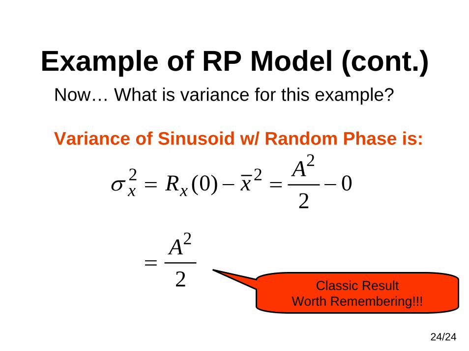
Example of RP Model (cont.)Now… What is variance for this example?

Variance of Sinusoid w/ Random Phase is:

2

02

)0(

2

222

A

AxRxx

=

−=−=σ

Classic Result Worth Remembering!!!