CLASSIFICATION OF MRI DATA USING DEEP LEARNING AND GAUSSIANPROCESS-BASED MODEL SELECTION

Hadrien Bertrand?† Matthieu Perrot† Roberto Ardon† Isabelle Bloch?

? LTCI, Telecom ParisTech, Universite Paris-Saclay, Paris, France†Philips Research, France

ABSTRACTThe classification of MRI images according to the anatomical

field of view is a necessary task to solve when faced with the in-creasing quantity of medical images. In parallel, advances in deeplearning makes it a suitable tool for computer vision problems. Us-ing a common architecture (such as AlexNet) provides quite goodresults, but not sufficient for clinical use. Improving the model isnot an easy task, due to the large number of hyper-parameters gov-erning both the architecture and the training of the network, and tothe limited understanding of their relevance. Since an exhaustivesearch is not tractable, we propose to optimize the network first byrandom search, and then by an adaptive search based on GaussianProcesses and Probability of Improvement. Applying this methodon a large and varied MRI dataset, we show a substantial improve-ment between the baseline network and the final one (up to 20% forthe most difficult classes).

Index Terms— Deep Learning, Convolutional Neural Net-works, MRI, Classification, Model Selection, Gaussian Process

1. INTRODUCTION

In daily clinical practice, automatic analysis of medical images so asto determine the observed anatomy would produce significant ben-efits in terms of time and cost, given the large number of imagesacquired each day. This anatomical knowledge can 1) produce re-liable search tools on ever increasing datasets (currently based onmanually defined tags), supporting follow up of a specific patient’sanatomy or finding similar anatomies or pathologies; 2) automate theproduction of reports on findings (e.g. transcribing tumors location);3) automatically enrich exams to render an augmented visualizationto ease communication between clinicians and patients.

While the imaging modality (CT, MR, US, etc.) is reliably pro-vided by the acquisition systems, the information on the imagedanatomical region (chest, abdomen, spine, etc.) is given by man-ual annotations. Under the pressure of maximizing equipment ex-ploitation, this information is very prone to errors. Yet, for any otherfurther anatomical analysis, the reliability of this information is cru-cial. Thus, in the present work, we aim to automatically determinethe imaged anatomical region from the image content. Solving thisproblem within the whole variability of medical imaging (modalities,protocols, patient anatomy, pathologies, etc.) would require a datasetcurrently inaccessible. Thus, we choose to restrict our study to MRImodality which already encompasses many aspects of the variabil-ity of the initial problem (high variability of protocols, anatomies,etc.). Moreover, our target space is limited to four anatomical re-gions: spine, head, abdomen and pelvis.

The recent surge of popularity and successes of deep learning forcomputer vision tasks has led to a wealth of applications, including

in medical imaging [1]. The commonly adopted approach for clas-sification tasks is to retrain a popular network model (AlexNet [2],VGG [3], etc.) on a specific dataset (sometimes just retraining thelast few layers). While this strategy provides often correct results onsmall and controlled datasets, it reveals insufficient when confrontedto the high variability of actual clinical data. This is the case of ourdataset, which is only built from such day to day clinical images.Given the high number of degrees of freedom and their correlatedimpact on network model performances, handcrafting better modelsoften proves very time consuming and inefficient.

In this paper, starting from a baseline network (Section 2.1), wepresent an automatic strategy to find better architectures given ourclinical context. We constrain our search to a space of networksrepresented by a specific parametrization (Section 2.2) that includesenough diversity and, at the same time, promising models (includingAlexNet-like, VGG-like). Inspired by the work in [4], we devise anautomatic optimization process (Section 2.3) to produce an ensembleof successful models (Section 2.4). The interest and efficiency of thisstrategy are demonstrated on our application in Section 3.

2. METHOD

Under the condition that each MRI volume can be classified as oneof our targeted anatomies (separating a volume into several ones ifit covers several parts of the anatomy), and since MRI data are ac-quired in a slice by slice approach, we reduce the anatomical re-gion prediction problem to a two dimension classification task (intoabdomen, pelvis, head and spine). Assuming that information con-tained in a slice is rich enough, we effectively augment our datasetsize. At the cost of loosing 3D information, we tend to a standard2D-image classification problem, a good candidate for Deep Learn-ing standard techniques.

2.1. Handcrafted Baseline Architecture

Several successful deep learning experiments in medical imaging areobserved using architectures inspired by AlexNet [2] or VGG [3] (re-fer in particular to this special issue of TMI: [1]). Following thesesteps, after tedious parameter tuning, we converged to a model pre-senting a quite satisfactory behavior on our problem, but, at the sametime, very difficult to further improve. Using the standard terms usedby the deep learning community [5], this baseline model consists of 5blocks, each comprising a convolution layer of 64 filters of size 3×3,followed by a rectified linear unit (ReLu) activation function and amax-pooling layer. The network ends with 2 fully-connected layers(resp. 4096 and 1024 units) interleaved with ReLU activations andterminated with a softmax decision layer. This network was trainedby minimizing the categorical cross-entropy loss weighted by class

978-1-5090-1172-8/17/$31.00 ©2017 IEEE 745

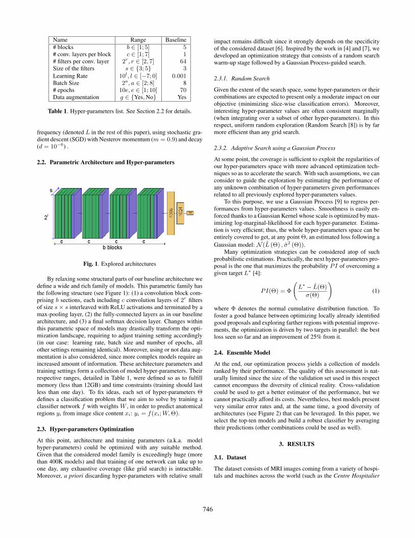
Name Range Baseline# blocks b ∈ [1; 5] 5# conv. layers per block c ∈ [1; 7] 1# filters per conv. layer 2r, r ∈ [2, 7] 64Size of the filters s ∈ {3; 5} 3Learning Rate 10l, l ∈ [−7; 0] 0.001Batch Size 2a, a ∈ [2; 8] 8# epochs 10e, e ∈ [1; 10] 70Data augmentation g ∈ {Yes,No} Yes

Table 1. Hyper-parameters list. See Section 2.2 for details.

frequency (denoted L in the rest of this paper), using stochastic gra-dient descent (SGD) with Nesterov momentum (m = 0.9) and decay(d = 10−6) .

2.2. Parametric Architecture and Hyper-parameters

Fig. 1. Explored architectures

By relaxing some structural parts of our baseline architecture wedefine a wide and rich family of models. This parametric family hasthe following structure (see Figure 1): (1) a convolution block com-prising b sections, each including c convolution layers of 2r filtersof size s× s interleaved with ReLU activations and terminated by amax-pooling layer, (2) the fully-connected layers as in our baselinearchitecture, and (3) a final softmax decision layer. Changes withinthis parametric space of models may drastically transform the opti-mization landscape, requiring to adjust training setting accordingly(in our case: learning rate, batch size and number of epochs, allother settings remaining identical). Moreover, using or not data aug-mentation is also considered, since more complex models require anincreased amount of information. These architecture parameters andtraining settings form a collection of model hyper-parameters. Theirrespective ranges, detailed in Table 1, were defined so as to fulfillmemory (less than 12GB) and time constraints (training should lastless than one day). To fix ideas, each set of hyper-parameters Θdefines a classification problem that we aim to solve by training aclassifier network f with weights W , in order to predict anatomicalregions yi from image slice content xi: yi = f(xi;W,Θ).

2.3. Hyper-parameters Optimization

At this point, architecture and training parameters (a.k.a. modelhyper-parameters) could be optimized with any suitable method.Given that the considered model family is exceedingly huge (morethan 400K models) and that training of one network can take up toone day, any exhaustive coverage (like grid search) is intractable.Moreover, a priori discarding hyper-parameters with relative small

impact remains difficult since it strongly depends on the specificityof the considered dataset [6]. Inspired by the work in [4] and [7], wedeveloped an optimization strategy that consists of a random searchwarm-up stage followed by a Gaussian Process-guided search.

2.3.1. Random Search

Given the extent of the search space, some hyper-parameters or theircombinations are expected to present only a moderate impact on ourobjective (minimizing slice-wise classification errors). Moreover,interesting hyper-parameter values are often consistent marginally(when integrating over a subset of other hyper-parameters). In thisrespect, uniform random exploration (Random Search [8]) is by farmore efficient than any grid search.

2.3.2. Adaptive Search using a Gaussian Process

At some point, the coverage is sufficient to exploit the regularities ofour hyper-parameters space with more advanced optimization tech-niques so as to accelerate the search. With such assumptions, we canconsider to guide the exploration by estimating the performance ofany unknown combination of hyper-parameters given performancesrelated to all previously explored hyper-parameters values.

To this purpose, we use a Gaussian Process [9] to regress per-formances from hyper-parameters values. Smoothness is easily en-forced thanks to a Gaussian Kernel whose scale is optimized by max-imizing log-marginal-likelihood for each hyper-parameter. Estima-tion is very efficient; thus, the whole hyper-parameters space can beentirely covered to get, at any point Θ, an estimated loss following aGaussian model: N (L (Θ) , σ2 (Θ)).

Many optimization strategies can be considered atop of suchprobabilistic estimations. Practically, the next hyper-parameters pro-posal is the one that maximizes the probability PI of overcoming agiven target L∗ [4]:

PI(Θ) = Φ

(L∗ − L(Θ)

σ(Θ)

)(1)

where Φ denotes the normal cumulative distribution function. Tofoster a good balance between optimizing locally already identifiedgood proposals and exploring farther regions with potential improve-ments, the optimization is driven by two targets in parallel: the bestloss seen so far and an improvement of 25% from it.

2.4. Ensemble Model

At the end, our optimization process yields a collection of modelsranked by their performance. The quality of this assessment is nat-urally limited since the size of the validation set used in this respectcannot encompass the diversity of clinical reality. Cross-validationcould be used to get a better estimator of the performance, but wecannot practically afford its costs. Nevertheless, best models presentvery similar error rates and, at the same time, a good diversity ofarchitectures (see Figure 2) that can be leveraged. In this paper, weselect the top-ten models and build a robust classifier by averagingtheir predictions (other combinations could be used as well).

3. RESULTS

3.1. Dataset

The dataset consists of MRI images coming from a variety of hospi-tals and machines across the world (such as the Centre Hospitalier

746

Fig. 2. Architecture of the 5 best models. Height represents the number of filters per layer, depth the size of the filters.

Fig. 3. A selection of axial and coronal abdomen slices showing thediversity and the complexity of our dataset.

Body Part # Volumes # SlicesAbdomen 282 11532Head 301 9032Pelvis 225 8854Spine 386 7732

Table 2. Content of the dataset.

Lyon-Sud, France or Johns Hopkins University, USA). As a conse-quence our images display a large variety of protocols (see Figure 3)as well as resolution and number of slices per volume. In this paper,the considered regions are limited to: abdomen, head, pelvis andspine (table 2 sums up the content of our dataset).

Our dataset is splitted in a training set for the optimization of theweights W , a validation set for model selection (optimization w.r.thyper-parameters) and a test set for model evaluation (resp. 50%,25%, 25%). The separation is done volume-wise to take into ac-count intra-subject slices correlations. Volumes containing multipleclasses are split by anatomical regions and can end up in differentsets. This raises the difficulty of the task since, in case of overfit-ting, predictions will be wrong at validation or testing phases. Wealso stratified classes across sets, giving us a proportion of slices perclass close to the proportion of volumes per class.

Finally, each slice is subject to a unique step of preprocessing: itis resized to 64×64 pixels, a good trade-off between time constraintsand quality of information.

Data augmentation consists in generating 80 000 images perepoch, which is 4 times as many images as the training set. The aug-mentation is done by applying translations, shearing and rotations,zooming, and adding noise.

3.2. Hyper-parameters Optimization

The hyper-parameters were optimized in two steps, 47 iterations ofrandom search followed by an adaptive search (as described in Sec-tion 2.3.2). The entire process is depicted in Figure 4. Adaptive

Fig. 4. Loss (left) and error rates (right) on validation dataset infunction of the number of models considered so far by the optimiza-tion process. In green: running median, in solid red: running min,in dashed red: baseline performance, in dashed black: iteration fromwhich random search is stopped in favor of adaptive search.

search presents quickly an important increase of the proportion ofmodels with good performance (supported by the decreasing run-ning median of the loss). Thus, selected combinations are on averagebetter than random search.

Many proposals present both a high loss and a high error rate.These correspond to models that put all images in the same class, inthis case: abdomen, which accounts for around 30% of the dataset(implying 70% of error rate).

3.3. Test Accuracy

Figure 2 shows the architecture of some of the best models chosenfor our ensemble. Despite the first two differing only in the num-ber of blocks, others display variations across all hyper-parametersexcept data augmentation, which is always turned on. The learningrate is in a small range, either 0.0001 or 0.001, and the batch size issmall (less than 16). Those networks tend to be deep (min. 8 convo-lutional layers) and the other hyper-parameters use a wide range ofvalues.

In terms of accuracy, the ensemble is slightly better than the bestmodel alone, however the ensemble benefits from a reduced bias.

Figure 5 shows the confusion matrices on the test set of the base-line and the ensemble of the 10 best models, demonstrating a sub-stantial improvement on the classification of all anatomical regions.Most of the errors come from pelvis and abdomen, which was ex-pected since the delimitation between those regions is ill-defined. Inboth cases pelvis is the class with the highest error.

For the volume classification, the choice of class is done by amajority vote on all slices of the volume. This gives us a higheraccuracy. The ensemble misclassifies 444 slices from 71 volumes,but only 7 volumes produce errors. The misclassified slices usually

747

Fig. 5. Confusion matrices on the test set, for the baseline network(left) and the ensemble (right), computed on slices (first row) and onvolumes (second row).

correspond to the first or last one of a volume, containing little infor-mation or being nearly part of another anatomical region.

3.4. Slice by slice analysis of a volume

Fig. 6. Slice by slice classification on a full body volume. Top:Class probabilities. Filled areas correspond to decision made whenthe probability is higher than 0.7. Bottom: Volume and ground truth.

As an interesting example, we analyzed a full body volume byclassifying each of its slices through our ensemble model. For eachslice, the predicted class is the one with a probability higher than0.7, and if no class meets this criterion, then we do not choose any.As we can see in Figure 6, the network is doing well at identifyingthe abdomen and the head. It also identifies correctly the pelvis,with some uncertainty. No class is dominant for most of the legs,however the feet are considered as spine with high probability. Italso mistakenly identifies the neck as pelvis.

Those mistakes could be corrected by using a more complex de-cision criterion than a simple probability cutoff. We also expect thatadding more anatomical regions to our dataset will allow for a betterlocalization of the present regions.

4. DISCUSSION AND CONCLUSION

To the problem of finding more accurate networks than handcraftedones, we have answered with two viable strategies. Random searchis as easy to implement as grid search and quickly improves onthe baseline, which makes it perfect for time-constrained situations.Without this constraint and at a higher cost in implementation, anadaptive search based on Gaussian Processes explores a range ofhighly accurate models suited for ensembling.

For the hyper-parameters where there is a “correct” answer, suchas the learning rate (0.001) and the presence of data augmentation,the guided search quickly converges and most models inherit theirvalues. We should remove them on further analysis and instead ex-plore a wider range of architectures by adding hyper-parameters con-trolling the fully-connected layers, such as the number of units, thenumber of layers, adding new types of layers such as dropout andbatch normalization placed across the network or even explore otherlearning method such as RMSProp or Adadelta.

One limitation of the current system is that some hyper-parameters depend on the value of others. For example we areunable to choose a different number of filters per layer as thenumber of layers is not fixed. We also limited the range of somehyper-parameters such as the filter size so as to have networks thatwould fit in memory and be trained in a reasonable amount of time.Only a subset of values combinations would cause a failure. Furtherwork could incorporate constraints on time and memory either byprecise estimations when possible or by measures during training toproduce estimations with a GP.

Results on volume classification were very satisfactory. Sinceit is done at slice level, we have obtained a decent localization toolwhich shows the robustness of our ensemble. Further work will fo-cus on adding more anatomical regions, which might require split-ting slices in patches to identify smaller regions such as organs.

5. REFERENCES

[1] “Special Issue on Deep Learning in Medical Imaging,” IEEETransactions on Medical Imaging, vol. 35, no. 5, 2016.

[2] A. Krizhevsky, I. Sutskever, and G. E. Hinton, “ImageNet Clas-sification with Deep Convolutional Neural Networks,” in Ad-vances in Neural Information Processing Systems 25, pp. 1097–1105. 2012.

[3] K. Simonyan and A. Zisserman, “Very Deep Convolutional Net-works for Large-Scale Image Recognition,” arXiv, 2014.

[4] D. R. Jones, “A Taxonomy of Global Optimization MethodsBased on Response Surfaces,” Journal of Global Optimization,vol. 21, no. 4, pp. 345–383, 2001.

[5] I. Goodfellow, Y. Bengio, and A. Courville, “Deep learning,”The MIT Press, 2016.

[6] J. Bergstra and Y. Bengio, “Random Search for Hyper-parameter Optimization,” The Journal of Machine Learning Re-search, vol. 13, pp. 281–305, 2012.

[7] J. Snoek, H. Larochelle, and R. P. Adams, “Practical BayesianOptimization of Machine Learning Algorithms,” in Advances inNeural Information Processing Systems, 2012, pp. 2951–2959.

[8] R. L. Anderson, “Recent advances in finding best operating con-ditions,” Journal of the American Statistical Association, vol.48, no. 264, pp. 789–798, 1953.

[9] C. E. Rasmussen and C. K. I. Williams, Gaussian Processes forMachine Learning, The MIT Press, 2005.

748