Embed Size (px)
Citation preview

CLASSIFICATION OF ELECTROENCEPHALOGRAM
(EEG) SIGNAL BASED ON FOURIER TRANSFORM
AND NEURAL NETWORK
PULOMA PRAMANICK (109EE0640)
Department of Electrical Engineering
National Institute of Technology Rourkela

CLASSIFICATION OF ELECTROENCEPHALOGRAM
(EEG) SIGNAL BASED ON FOURIER TRANSFORM
AND NEURAL NETWORK
A Thesis submitted in partial fulfillment of the requirements for the degree of
Bachelor of Technology in “Electrical Engineering”
By
PULOMA PRAMANICK (109EE0640)
Under guidance of
Prof. SUBHOJIT GHOSH
Department of Electrical Engineering
National Institute of Technology
Rourkela-769008 (ODISHA)
May-2013

DEPARTMENT OF ELECTRICAL ENGINEERING
NATIONAL INSTITUTE OF TECHNOLOGY, ROURKELA
ODISHA, INDIA-769008
CERTIFICATE
This is to certify that the thesis entitled “Classification of Electroencephalogram(EEG) signal
based on Fourier transform and neural network”, submitted by Puloma Pramanick(Roll
No. 109EE0640) in partial fulfilment of the requirements for the award of Bachelor of
Technology in Electrical Engineering during session 2012-2013 at National Institute of
Technology, Rourkela, is a bonafide record of research work carried out by her under my
supervision and guidance.
The candidate has fulfilled all the prescribed requirements.
The Thesis which is based on candidate’s own work, has not submitted elsewhere for a
degree/diploma.
In my opinion, the thesis is of standard required for the award of a bachelor of technology degree
in Electrical Engineering.
Place: Rourkela
Dept. of Electrical Engineering Prof. Subhojit Ghosh
National institute of Technology Assistant Professor
Rourkela-769008

ACKNOWLEDGEMENTS
I am very thankful to my guide Prof. Subhojit Ghosh for his valuable help. He is always there to
show the right track, when needed his help. It is with the help of his valuable suggestions,
guidance and encouragement, that I am able to perform this project work.
Puloma Pramanick
B.Tech (Electrical Engineering)

ABSTRACT
Human normal and epileptic electroencephalogram (EEG) signals have been analysed
using Fourier Transform (FT). The area under the spectrum of both normal and epileptic EEG is
calculated as feature for classification. The classification is done with the help of neural network
(Levenberg - Marquardt algorithm).Our final goal of the study is the automatic detection of the
epileptic disorders in the EEG in order to support the diagnosis and care of the epileptic
syndromes and related seizure disorders.

CONTENTS
Abstract
Contents
List of Figures
List of Tables
CHAPTER 1
INTRODUCTION
1.1 Introduction
1.1.1 Activities of the neuron
1.1.2 Recording of the EEG signals
1.1.3 Frequency bands of the EEG signal
1.2 Objective
1.3 Organisation of Thesis
CHAPTER 2
DATASET AND FEATURE EXTRACTION
2.1 Dataset
2.2 Pre-processing
2.3 Fourier Analysis
2.4 Feature Extraction
CHAPTER 3
ARTIFICIAL NEURAL NETWORK
3.1 Background
3.2 Feed-forward Neural Network

3.3 Back-propagation Training
3.4 Data Series Partitioning
CHAPTER 4
RESULTS
4.1 Results
CHAPTER 5
CONCLUSIONS

LIST OF FIGURES
Fig. No Name of the Figure
1.1 Structure of a neuron
2.1 EEG signal for the sets F, N, O, S and Z (magnitude in microvolts).
2.2 Frequency spectrum of the EEG signals for the sets F, N, O, S and Z
3.1 Neural network architecture
3.2 Sigmoid activation function
4.1 Iterative variation of the mean square error between the actual output and a
trained network with a single hidden layer of 20 neurons
4.2 Iterative variation of the mean square error between the actual output and a
trained network with two hidden layers, each of 20 and 5 neurons
4.3 Iterative variation of the mean square error between the actual output and a
trained network with three hidden layers, each of 20, 10 and 5 neurons

LIST OF TABLES
Table. No. Name of the Table
2.1 Area under different sub-bands of the frequency spectrum (Z set)
2.2 Area under different sub-bands of the frequency spectrum (O set)
2.3 Area under different sub-bands of the frequency spectrum (F set)
2.4 Area under different sub-bands of the frequency spectrum (N set)
2.5 Area under different sub-bands of the frequency spectrum (S set)
4.1 Structure of the neural network and accuracy achieved with the trained network

CHAPTER 1
Introduction

1.1 INTRODUCTION
The electroencephalogram (EEG) consists of a time series data of evoked potentials
resulting from the systematic neural activities in a brain. The recording data of the human EEGs
are carried out by placing the electrodes [1] on the scalp, and plotted as voltage magnitude
against time. The voltage of the EEG signal corresponds to its amplitude. The general voltage
range of the scalp EEG lie between 10 and 100 µV, and in adults more frequently in the range of
10 and 50µV. In the frequency spectrum range of the EEG, the frequency range extends from
ultraslow to ultra-fast frequency components. The extreme frequency ranges play no significant
role in the clinical EEG. The general frequency range of interest lies between 0.1Hz and 100Hz
for the classification purpose. The frequency range is generally classified into several frequency
components, or delta rhythm (0.5 - 4Hz), theta rhythm (4 -8Hz), alpha rhythm (8 - 13Hz) and
beta rhythm (13- 30Hz). For normal adults, the slow ranges (0.3 -7Hz) and the very fast range
(>30Hz) are sparsely represented, and medium (8 - 13Hz) and fast (14 - 30Hz) components
predominate [2].
Since 1970, research in the automated seizure detection began [3] and various
algorithms are proposed for this problem [4]. These algorithms for automated detection of
epileptic seizures depend on the identification of various patterns such as an increase in
amplitude [5], sustained rhythmic activity [6], or EEG flattening [7]. Many of the algorithms
have been developed based on spectral features [8-11] or wavelet features [12- 16], amplitude
relative to background activity [17] and spatial context [17, 18]. Other features of chaotic [19,
20] include correlation dimension [21], entropy [22] and Lyapunov exponents [16,22] also
characterize the EEG signal. These features is used to classify the EEG signal using nearest
neighbor classifiers [24], decision trees [10], ANNs [16, 22], support vector machines (SVMs)
[11,16] or adaptive neuro-fuzzy inference systems [14,15,22] in order to identify the occurrence
of seizures.
We have analyzed the human normal and epileptic EEG signals from the waveform
and periodicity using the Fourier transform (FT) in order to test their abilities to detect localized
characteristic frequency component in EEG and extract features from them. Then, these features
are used to classify the segments concerning the presence or absence of epileptic seizures.

1.1.1 Activities of the Neuron
There are two types of cells in the Central Nervous System (CNS), nerve cells and
glia cells. The nerve cell consists of axons, dendrites and cell bodies. The cylindrical shaped
axon transmits the electrical impulse. Dendrites are connected to the axons or dendrites of other
inside cells and receive the electrical impulse from other nerves cells. Each nerve of human is
approximately connected to 10000 other nerves [25]. The electrical activity is mainly due the
current flow between the tip of dendrites and axons, dendrites and dendrites of cells. The level of
these signals is in V range and its frequency is less than 100Hz [25].
Figure 1.1 Structure of a neuron [25]
1.1.2 Recording of EEG signals
EEG is recorded from many electrodes arranged in a particular pattern or montage. A
common standard called the International 10/20 System is used here. These methods are cheap
and give a continuous record of brain activity with better than millisecond resolution. This tool
can achieve the high temporal resolution and for this reasons the detailed discoveries of dynamic
cognitive processes have been reported using EEG and ERP (Event Related Potentials) methods.

1.1.3 Frequency bands of the EEG signal
Most of EEG waves range from 0.5-500Hz, however the following four frequency
bands are clinically relevant: (i) delta, (ii) theta, (iii) alpha and (iv) beta
Delta waves: Delta waves frequency is up to 3 Hz. It is slowest wave having highest amplitude.
It is dominant in infants up to one year and adults in deep sleep.
Theta waves: It is a slow wave with frequency range from 4 Hz to 7 Hz. It emerges with closing
of the eyes and with relaxation. It is normally seen in young children and in adults.
Alpha waves: Alpha has frequency range from 7 Hz to 12 Hz. It is most commonly seen in
adults. Alpha activity occurs rhythmically on both sides of the head. Alpha wave appears with
closing eyes (relaxation state) and disappears normally with opening eyes/stress. It is treated as a
normal waveform.
Beta waves: Beta activity is fast with small amplitude. It has frequency range from 14 Hz to 30
Hz. It is dominant in patients who are alert or anxious or who have their eyes open. Beta waves
usually seen on both sides in symmetrical distribution and is most evident frontally. It is a
normal rhythm and observed in all age groups. These mostly appear in frontal and central portion
of the brain. The amplitude of the beta wave is less than 30μV [25].
1.2 OBJECTIVE
The objective is to analyse the human normal and epileptic EEG signals using signal
processing tools and classify them into different classes. To achieve this,
(i) Fourier analysis is done on both normal and epileptic EEG signals,
(ii) Features are extracted based on area under the spectrum,
(iii) Signals are classified with the help of Artificial Neural Network classifier.
1.3 ORGANISATION OF THESIS
Chapter 1 outlines the basic theory of the EEG signals.
Chapter 2 discusses about the data collected, pre-processing, feature extraction and classification
of the EEG signals.
Chapter 3 discusses the results obtained.
Chapter 4 summarizes the conclusion and references.

CHAPTER 2
Dataset and Feature Extraction

2.1 DATASET
We used the dataset described in reference [26]. The complete dataset consists of five
sets (denoted as Z, O, N, F and S) each containing 100 single-channel EEG segments each
having 23.6 sec duration. Sets Z and O have been taken from surface EEG recordings of five
healthy volunteers with eye open and closed, respectively. Signals in the two sets have been
measured in seizure-free intervals from five patients in the epileptogenic zone (F) and from the
hippocampal formation of the opposite hemisphere of the brain (N). Set S contains seizure
activity. Here, all the sets are used.
Figure 2.1: EEG signal for the sets F, N, O, S and Z [26] (magnitude in microvolts).

Figure 2.2: Frequency spectrum of the EEG signals for the sets F, N, O, S and Z [26].
2.2 PRE-PROCESSING
The application of a FIR [27] filter of 30 Hz, is regarded as the first step of analysis.
Signal pre-processing is necessary to maximize the signal-to-noise ratio (SNR) because there are
many noise sources encountered with the EEG signal. Noise sources can be non-neural (eye
movements, muscular activity, 50Hz power-line noise) or neural (EEG features other than those
used for control). Further pre-processing was not performed because the purpose is to be as close
as possible for real-time applications and pre-processing would slowdown the process of data
analysis. Moreover, data recorded outside the laboratory are likely to be noisier than those
recorded inside. So it is assumed that processing noisier data would have better generalization
properties.

2.3 FOURIER ANALYSIS
Discrete fourier transform:
( ) ∑ ( ) ( )( )
(2.1)
( ) ( )∑ ( ) ( )( )
(2.2)
where = ( )
is the Nth
root of unity.
The Fast Fourier Transform (FFT) is simply a fast (computationally efficient) way to
calculate the Discrete Fourier Transform (DFT) which reduces the number of computations
needed for N points from 2N2 to 2NlgN, where lg is the base-2 logarithm.
To compute an N-point DFT when N is composite (that is, when N=N1N2 ), the
problem is sovled using the Cooley-Tukey algorithm [28], which first computes N1 transforms
of size N2 , and then computes N1 transforms of size N2 . The decomposition is to be applied
recursively to both the N1- and N2 -point DFTs until the problem is solved using one machine-
generated fixed-size "codelets". The codelets then use several algorithms in combination, such as
a variation of Cooley-Tukey [30], a prime factor algorithm [31], and a split-radix algorithm [29].
The particular factorization of N is chosen heuristically.
When N is a prime number, an N-point problem is decomposed into three (N-1)-point
problems using Rader's algorithm [32]. It then uses the Cooley-Tukey decomposition described
above to compute the (N-1)-point DFT. For most N, real-input DFTs require roughly half the
computation time of complex-input DFTs. The execution time for FFT depends on the length of
the transform. It is fastest for powers of two.
2.4 FEATURES EXTRACTION
Features are extracted for different bands. The feature used here is area under the
spectra. The area is calculated using the trapezoidal rule. In numerical analysis, the trapezoidal

rule (also known as the trapezoid rule or trapezium rule) is a technique for approximating
the definite integral
∫ ( )
(2.3)
The trapezoidal rule works by approximating the region under the graph of the
function f(x) as a trapezoid and calculating its area. It follows that
∫ ( ) ( )(( ( ) ( )) )
(2.4)
Area of the frequency bands (delta, theta, alpha, beta) are calculated for each EEG segments.
There are 100 EEG segments in each set.
For example, only ten values for each set are shown.
Frequency Bands
Sl. No.
of
EEG data
1 1.6090 0.0968 0.0697 2.0751
2 2.1102 0.1515 0.1014 2.6351
3 1.6851 0.1152 0.0790 2.2138
4 2.1054 0.2680 0.1650 3.7274
5 1.6558 0.1632 0.1090 2.1241
6 1.8004 0.1133 0.0711 2.3644
7 2.0154 0.1357 0.0989 3.4960
8 1.3267 0.0781 0.0499 1.9388
9 1.0111 0.1119 0.0765 1.4273
10 1.2582 0.0911 0.0640 1.6643
Table 2.1: Area under different sub-bands of the frequency spectrum (Z set).

Frequency Bands
Sl. No.
of
EEG data
1 1.8023 0.1475 0.0972 2.1722
2 1.7660 0.1001 0.0659 1.9112
3 2.0737 0.1131 0.0814 2.5793
4 2.4891 0.1218 0.0889 2.8784
5 2.2747 0.0976 0.0686 2.2707
6 2.0332 0.1948 0.1274 2.3489
7 2.3861 0.1227 0.0809 1.9850
8 1.8757 0.1065 0.0786 2.3671
9 1.9817 0.1015 0.0681 1.9499
10 3.5417 0.1478 0.1005 3.6591
Table 2.2: Area under different sub-bands of the frequency spectrum (set O).
Frequency Bands
Sl. No.
of
EEG data
1 0.6675 0.0736 0.0459 0.7107
2 1.9032 0.0913 0.0590 1.5143
3 2.4944 0.0829 0.0554 1.6491
4 0.9838 0.0787 0.0479 0.6794
5 2.7019 0.1897 0.1178 3.2943
6 0.6508 0.0587 0.0351 0.5404
7 1.2585 0.1329 0.0789 1.2961
8 2.0523 0.0713 0.0460 0.9778
9 8.8239 0.4322 0.3265 3.9499
10 2.5738 0.1035 0.0742 1.9110
Table 2.3: Area under different sub bands of the frequency spectrum (set F).

Frequency Bands
Sl. No.
of
EEG data
1 1.1659 0.0640 0.0420 0.7205
2 1.5301 0.0942 0.0647 1.1614
3 1.2224 0.1034 0.0648 1.1079
4 1.1150 0.1012 0.0670 0.9082
5 4.1540 0.4466 0.2776 5.2455
6 1.2557 0.0853 0.0545 1.0953
7 0.9313 0.0872 0.0559 0.9377
8 0.8588 0.0776 0.0499 .7275
9 1.5266 0.1274 0.0829 1.3612
10 0.9322 0.0623 0.0399 0.8706
Table 2.4: Area under different sub-bands of the frequency spectrum (set N).
Frequency Bands
Sl.No.
of
EEG data
1 20.3300 0.9862 0.7205 20.6770
2 21.7060 1.2177 0.8595 21.8050
3 17.4810 0.7699 0.5015 22.6240
4 6.36170 0.1828 0.1241 4.03300
5 12.2130 0.5927 0.3809 9.32790
6 4.98120 0.1557 0.1097 4.19029
7 9.17380 1.4740 1.1305 21.8920
8 14.4450 0.4538 0.3218 7.92038
9 14.4860 0.5674 0.3932 10.9850
10 27.5000 1.6397 1.1746 43.0630
Table 2.5: Area under different sub-bands of the frequency spectrum (set S).

CHAPTER 3
Artificial Neural Network
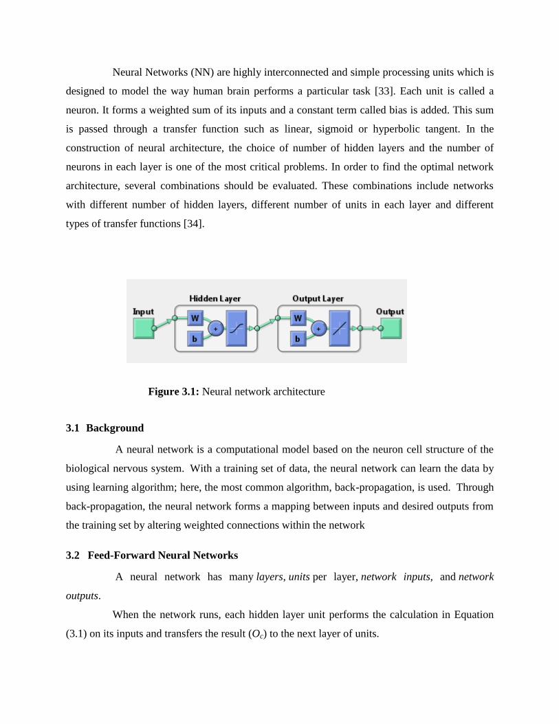
Neural Networks (NN) are highly interconnected and simple processing units which is
designed to model the way human brain performs a particular task [33]. Each unit is called a
neuron. It forms a weighted sum of its inputs and a constant term called bias is added. This sum
is passed through a transfer function such as linear, sigmoid or hyperbolic tangent. In the
construction of neural architecture, the choice of number of hidden layers and the number of
neurons in each layer is one of the most critical problems. In order to find the optimal network
architecture, several combinations should be evaluated. These combinations include networks
with different number of hidden layers, different number of units in each layer and different
types of transfer functions [34].
Figure 3.1: Neural network architecture
3.1 Background
A neural network is a computational model based on the neuron cell structure of the
biological nervous system. With a training set of data, the neural network can learn the data by
using learning algorithm; here, the most common algorithm, back-propagation, is used. Through
back-propagation, the neural network forms a mapping between inputs and desired outputs from
the training set by altering weighted connections within the network
3.2 Feed-Forward Neural Networks
A neural network has many layers, units per layer, network inputs, and network
outputs.
When the network runs, each hidden layer unit performs the calculation in Equation
(3.1) on its inputs and transfers the result (Oc) to the next layer of units.

Activation function of a hidden layer unit is given by
= (∑ ) (3.1)
where
( ) ( )
Oc = the output of the current hidden layer unit c,
P = either the number of units in the previous hidden layer or number of network inputs,
ic,p = an input to unit c from either the previous hidden layer unit p or network input p,
wc,p = the weight modifying the connection from either unit p to unit c or from input p to unit c,
and
bc = the bias.
In Equation (3.1), hHidden(x) is the sigmoid activation function of the unit and is shown
in Figure 3.2. The training data must be scaled appropriately to avoid saturation which can make
the training of the network difficult. Similarly, the weights and biases are initialized to
appropriately scaled values before training.
Figure 3.2: Sigmoid activation function.
3.3 Back-propagation Training
The neural network has to be trained on data series. <input, output> pairs are
extracted from data series, where input and output are vectors equal in size to the number of
network inputs and outputs, respectively. Back-propagation training has three steps:
1. Present an input vector to the network inputs and run the network: activation
functions are sequentially computed in the forward direction from the first hidden
layer to the output layer

2. Compute the difference between the desired output for that data series, output,
and the actual network output (output of unit(s) in the output layer). The error is
sequentially propagated backward from the output layer to the first hidden layer
3. For every connection, change the weight modifying that connection in
proportion to the error.
3.4 Data Series Partitioning
The method for training a network is to first divide the data series into three disjoint
sets: training set, validation set, and test set. The network is trained (e.g., with back-
propagation) with training set, its generalization ability is monitored on the validation set, and its
ability to forecast is tested on the test set. Network should avoid overfitting. Overfitting occurs
when the network is blindly trained. A network that has overfit the training data is said to have
poor generalization ability.

CHAPTER 4
Results

4.1 RESULTS
In the classification stage, the area under the spectrum features are applied as input to
feed-forward neural network. The feed-forward back-propagation network has been implemented
using Lavenberg-Marquardt optimization algorithm. The algorithm involves minimization of the
error by updating the network and bias using damped least squares. It interpolates between the
Gauss Newton algorithm and the method of gradient descent. The total dataset consisting of 500
patterns has been divided into training and testing set of 400 and 100 patterns respectively. In the
present work, the network with four input and one output neurons is created using the newff
command in MATLAB. The accuracy of the network trained in correctly classifying the test
patterns into two groups i.e., seizure and healthy.
Different combination of network structures (hidden layer and neurons) was tested
through pilot runs. Table 4.1 reports the accuracy of ANN with three different combinations of
hidden layer and neurons. The vector corresponding to the structure in the first column refers to
the number of hidden neurons in each hidden layer i.e. [20,5] refers to the two hidden layer each
with twenty and five neurons. Since the training phase involves initialization with random
weights, different execution of the training algorithm leads to different network and hence
different accuracy. The results reported in Table 4.1 refer to the best accuracy obtained for five
runs of algorithm. The corresponding iterative variation of the mean square error between the
network and actual output is displayed in figures 4.1-4.3 respectively.
Table 4.1: Structure of the neural network and accuracy achieved with the trained network
Structure of the neural network Accuracy
[20] 98
[20,5] 99
[20,10,5] 99

Figure 4.1 Iterative variation of the mean square error between the actual output and a trained
network with a single hidden layer of 20 neurons.
Figure 4.2 Iterative variation of the mean square error between the actual output and a trained
network with two hidden layer of each of 20 and 5 neurons.

Figure 4.3 Iterative variation of the mean square error between the actual output and a trained
network with three hidden layer, each of 20, 10 and 5 neurons

CHAPTER 5
Conclusion
Epileptic seizures are manifestations of epilepsy. The detection of epileptiform
discharges in the EEG is an important component in the diagnosis of epilepsy. The present
works aim at classifying the EEG pattern into two groups (seizure and healthy), based on the
area of the frequency spectrum under different sub-bands. After feature extraction, the
classification of the patterns based on the frequency spectrum features is carried out using a
neural network. The network based on the back-propagation algorithm is able to achieve an
accuracy of 99%. The algorithm is found to be highly sensitive to initial weight and network
structure. Future work in this direction is planned on the use of optimization algorithms for
determining the optimal structure of the neural and network.

REFERENCES:
[1] Sinha RK, EEG power spectrum and neural network based sleephypnogram analysis for a
model of heat stress. J Clin Monit Comput 2008; 22:261–268
[2] E. Niedermeyer, “Epileptic seizure disorders” Chapter 27, in E. Niedermeyer and F.L. da
Silva ed. “Electroencephalography: Basic principles, Clinical applications, and Related
fields”, Fourth edition. Lippincott Willams & Wilkins, Philadelphia (1999).
[3] Alexandros T. Tzallas, Markos G. Tsipouras, Dimitrios I. Fotiadis, “A Time-Frequency
Based Method for the Detection of Epileptic Seizures in EEG Recordings”, Twentieth IEEE
International Symposium on Computer-Based Medical Systems (CBMS'07).
[4] J. Gotman, “Automatic detection of seizures and spikes,” J. Clin. Neurophysiol, vol. 16,
1999, pp. 130-40.
[5] P.F. Prior, R.S.M. Virden, and D.E. Maynard, “An EEG device for monitoring seizure
discharges,” Epilepsia, vol. 14 (4), 1973, pp. 367-72.
[6] W.R. S. Webber, R.P. Lesser, R.T. Richardson, and K. Wilson, “An approach to seizure
detection using an artificial neural network (ANN),” Electroenceph. Clin. Neurophysiol., vol.
98 (4), 1996, pp. 250-72.
[7] G.W. Harding, “An automated seizure monitoring system for patients with indwelling
recording electrodes”,Electroenceph. Clin. Neurophysiol., vol. 86 (6), 1993, pp. 428-37.
[8] V. Srinivasan, C. Eswaran, and N. Sriraam, “Artificial Neural Network Based Epileptic
Detection Using Time- Domain and Frequency Domain Features”, J. Med. Syst., vol.29 (6),
2005, pp. 647-60.
[9] V.P. Nigam, and D. Graupe, “A neural-network-based detection of epilepsy”, Neurol.
Res., vol. 26 (6), 2004, pp. 55-60.
[10] K. Polat, and S. Güneş, “Classification of epileptiform EEG using a hybrid system based
on decision tree classifier and fast Fourier transform”, Appl. Math. Comput., vol. 32 (2),
2007, pp 625-31.
[11] B. Gonzalez-Vellon, S. Sanei, and J.A. Chambers, “Support vector machines for seizure
detection”, in Proc. Of the 3rd IEEE Intern. Symp. on Sign. Proc. and Inf. Technol., 14-17
Dec. 2003, Germany, pp. 126- 29.
[12] H. Adeli, Z. Zhou, and N. Dadmehr, “Analysis of EEG records in an epileptic patient
using wavelet transform”, J. Neurosc. Meth., vol. 123 (1), 2003, pp. 69-87.
[13] A. Subasi, “Signal classification using wavelet feature extraction and a mixture of expert
model”, Exp. Syst. Appl., vol. 32 (4), 2007, pp. 1084-93.

[14] N. Sadati, H.R. Mohseni, and A. Magshoudi, “Epileptic Seizure Detection Using Neural
Fuzzy Networks”, in Proc. of the IEEE Intern. Conf. on Fuzzy Syst., 16-21 Jul. 2006,
Canada, pp. 596-600.
[15] İ. Güler and E.D. Übeyli, “Adaptive neuro-fuzzy inference system for classification of
EEG signals using wavelet coefficients”, J. Neurosc. Meth., vol. 148 (2), 2005, pp 113-21.
[16] I. Güler, and E.D. Übeyli, “Multiclass Support Vector Machines for EEG Signals
Classification”, IEEE Trans. Inform. Τechn. Biomed., in Press.
[17] A.A. Dingle, R.D. Jones, G.J. Caroll, and W.R. Fright, “A Multistage System to Detect
Epileptiform Activity in the EEG”, IEEE Trans. Biomed. Eng., vol. 40 (12), 1993, pp. 1260-
68.
[18] F.I. Argoud, F.M. De Azevedo, J.M. Neto, and E. Grillo, “SADE3: an effective system
for automated detection of epileptiform events in long-term EEG based on context
information”, Med. Biol. Eng. Comput., vol. 44 (6), 2006, pp. 459-70.
[19] L.D. Iasemidis, and J.C. Sackellares, “Chaos theory and epilepsy”, The Neurosc., vol. 2,
1996, pp. 118-26.
[20] N. Kannathal, U.R. Acharya, C.M. Lim, and P.K. Sadasivan, “Characterization of EEG-
A comparative study”, Comp. Meth. Prog. Biomed., vol. 80 (1), 2005, pp. 17-23.
[21] D.E. Lerner, “Monitoring changing dynamics with correlation integrals: case study of an
epileptic seizure”, Physica D, vol. 97 (4), 1996, pp. 563-76.
[22] N.F. Güler, E.D. Übeyli, and İ. Güler, “Recurrent neural networks employing Lyapunov
exponents for EEG signals classification”, Exp. Syst. Appl., vol. 29 (3), 2005, pp. 506-14.
[23] N. Kannathal, M.L. Choo, U.R. Acharya, and P.K. Sadasivan, “Entropies for detection
of epilepsy in EEG”, Comput. Meth. Prog. Biomed., vol. 80 (3), 2005, pp. 187-94.
[24] H. Qu, and J. Gotman, “A patient-specific algorithm for the detection of seizure onset in
long-term EEG monitoring: possible use as a warning device”, IEEE Trans. Biomed. Eng.,
vol. 44 (2), 1997, pp. 115-22.
[25] Saeid Sanei and J.A. Chambers, EEG Signal Processing, John Wiley and Sons Ltd,
England, 2007
[26] R.G. Andrzejak, K. Lehnertz, F. Mormann, C. Rieke, P. David, and C. E. Elger,
“Indications of nonlinear deterministic and finite-dimensional structures in time series of
brain electrical activity: Dependence on recording region and brain state,” Phys. Rev. E, vol.
64, 2001, pp. 061907 (1-8).
[27] Programs for Digital Signal Processing, IEEE Press, New York, 1979. Algorithm 5.2
[28] Cooley, J. W. and J. W. Tukey, "An Algorithm for the Machine Computation of the

Complex Fourier Series, "Mathematics of Computation, Vol. 19, April 1965, pp. 297-301.
[29] Duhamel, P. and M. Vetterli, "Fast Fourier Transforms: A Tutorial Review and a State
of the Art," Signal Processing, Vol. 19, April 1990, pp. 259-299.
[30] Oppenheim, A. V. and R. W. Schafer, Discrete-Time Signal Processing, Prentice-Hall,
1989, p. 611.
[31] Oppenheim, A. V. and R. W. Schafer, Discrete-Time Signal Processing, Prentice-Hall,
1989, p. 619.
[32] Rader, C. M., "Discrete Fourier Transforms when the Number of Data Samples Is
Prime," Proceedings of the IEEE, Vol. 56, June 1968, pp. 1107-1108.
[33] S. Haykin, Neural Networks: A Comprehensive Foundation, Prentice-Hall, New Jersey,
1999.
[34] Neural Network Toolbox; Users’ Guide (R2011b), Mathswork,2011.