Embed Size (px)
Citation preview

Classical Mechanics
Joseph Conlon
April 9, 2014

Abstract
These are the current notes for the S7 Classical Mechanics course as of 9thApril 2014. They contain the complete text and diagrams of the notes. Therewill be no more substantive revisions of these notes until Hilary 2014-15 (smalltypographical revisions may occur inbetween).

Contents
1 Course Summary 3
2 Calculus of Variations 5
3 Lagrangian Mechanics 103.1 Lagrange’s Equations . . . . . . . . . . . . . . . . . . . . . . . . . 103.2 Rotating Frames . . . . . . . . . . . . . . . . . . . . . . . . . . . 163.3 Normal Modes . . . . . . . . . . . . . . . . . . . . . . . . . . . . . 223.4 Particle in an Electromagnetic Field . . . . . . . . . . . . . . . . . 253.5 Rigid Bodies . . . . . . . . . . . . . . . . . . . . . . . . . . . . . . 273.6 Noether’s Theorem . . . . . . . . . . . . . . . . . . . . . . . . . . 30
4 Hamiltonian Mechanics 334.1 Hamilton’s Equations . . . . . . . . . . . . . . . . . . . . . . . . . 334.2 Hamilton’s Equations from the Action Principle . . . . . . . . . . 354.3 Poisson Brackets . . . . . . . . . . . . . . . . . . . . . . . . . . . 364.4 Liouville’s Theorem . . . . . . . . . . . . . . . . . . . . . . . . . . 394.5 Canonical Transformations . . . . . . . . . . . . . . . . . . . . . . 42
5 Advanced Topics 505.1 The Hamilton-Jacobi Equation . . . . . . . . . . . . . . . . . . . 505.2 The Path Integral Formulation of Quantum Mechanics . . . . . . 555.3 Integrable systems and Action/Angle Variables . . . . . . . . . . 60
2

Chapter 1
Course Summary
This course is the S7 Classical Mechanics short option (for physicists) and alsothe B7 Classical Mechanics option for those doing Physics and Philosophy.
It consists of 16 lectures in total, and aims to cover advanced classical me-chanics, and in particular the theoretical aspects of Lagrangian and Hamiltonianmechanics. Approximately, the first 12 lectures cover material that is examinablefor both courses, whereas the last four lectures (approximately) cove material thatis examinable only for B7.
General Comments
Why be interested in classical mechanics and why be interested in this course?Classical mechanics has a beautiful theoretical structure which is obscured simplyby a presentation of Newton’s laws along the lines of F = ma. One of the aimsof this course is to reveal this structure.
Another good reason for taking this course is to understand quantum me-chanics better.
‘What do they know of quantum mechanics who only quantum me-chanics know?’
The Lagrangian and Hamiltonian formulations of classical mechanics provide theclassical structures that map across to the different formulations of quantummechanics. Understanding advanced classical mechanics therefore allows you tounderstand quantum mechanics better, and to see how it differs and how it issimilar to classicla mechanics.
In particular, Lagrangian mechanics and the action principle translate nat-urally to the Feynman path integral formulation of quantum mechanics, andHamiltonian mechanics turns into the ‘canonical’ treatment of quantum mechan-ics, as for example taught in the second year quantum mechanics course.
3

Books
Classical mechanics is an old subject and there are many books on the topic, witha range of styles and quality. Here are some possibilities
1. Hand + Finch (Analytical Mechanics) - this has plenty of details and ex-amples, while not being short on the number of words.
2. Kibble + Berkshire (Classical Mechanics) - a decent book which is maybeslightly lower than the level of the course, as it takes a while to get toLagrangians
3. Landau + Liftshitz - vol I (Mechanics) - everyone should be exposed toLandau and Liftshitz at some point. It is quite terse, and with no verbosity,but a classic text.
4. Arnold - Mathematical Methods of Classical Mechanics - A mathemticallysophisticated approach to mechanics, above the level of the course.
5. Goldstein - a standard text for American graduate courses.
It is also worth consulting the lecture notes by the previous lecturers, John Magor-rian and James Binney, for a similar if different take on the precise material withinthe course.
Errata
Please send corrections to [email protected]. I thank Guillermo Vallefor corrections to an earlier version of these notes.
4

Chapter 2
Calculus of Variations
A function takes a number as input and gives (usually) a number as output.A functional takes a function as input and gives (usually) a number as output.We start with a well-defined mathematical problem. Suppose we have a set of
n coordinates, q1, q2, . . . qn, which are functions of time t. At any time there arealso the first derivatives of these coordinates, q1, q2, . . . qn. In classical mechanicsthe state of the system is set by the position and velocities: we need to knowboth to be able to predict the future evolution.
Now suppose we have a function (the notation L anticipates this being theLagrangian)
L(qi, qi, t). (2.1)
Given this function, we can define the functional S[f ] through
S =
∫ B
A
L(qi, q,t)dt (2.2)
S is called the action. Here A and B refer to initial and final conditions: Acorresponds to t = t0, qi = qi(t0) and B refers to t = tf , qi = qi(tf ).
We require that the path qi(t) between A and B be an extremum of theaction. This means that under a change in path of first order in smallness,qi(t) → qi(t) + δqi(t), the first order change in the action δS vanishes. Whatequations does this generate for qi(t)?
Suppose we vary the path slightly:
S + δS =
∫ B
A
L(qi(t) + δqi(t), qi(t) + δqi(t), t)
=
∫ B
A
L(qi(t), qi(t), t) +∑i
δqi(t)∂L∂qi
+∑i
δqi(t)∂L∂qi
dt. (2.3)
Now, we can write∑i
δqi(t)∂L∂qi
=d
dt
(∑i
δqi(t)∂L∂qi
)−∑i
δqi(t)d
dt
(∂L∂qi
).
5

This enables us to write
S + δS =
∫ B
A
L(qi(t), qi(t), t) +∑i
δqi(t)
(∂L∂qi
− d
dt
(∂L∂qi
))+
[δqi(t)
∂L∂qi
]BA
.
(2.4)However, by definition δqi(t) = 0 at A and B, and so we have
δS =
∫ B
A
∑i
δqi(t)
(∂L
∂qi− d
dt
(∂L
∂qi
))dt. (2.5)
This vanishes for arbitrary δqi(t) if and only if
d
dt
(∂L
∂qi
)− ∂L
∂qi= 0. (2.6)
Why? If ∫ x1
x0
f(x)g(x)dx = 0 (2.7)
for arbitrary f(x), then g(x) = 0.
To see this, prove it by contradiction. Suppose g(x) = 0 at some point x′. Then by making f(x) approach
the δ-function δ(x− x′), you should be able to see that we can make the integral continuously approach∫ x1
x0
δ(x− x′)g(x)dx = g(x
′) = 0. (2.8)
Therefore if g(x) is ever non-zero, we can find a form of f(x) that leads to a non-zero result for the integral.
This establishes the contradiction and explains the result.
It follows that paths qi(t) extremising S are those satisfying
d
dt
(∂L
∂qi
)− ∂L
∂qi= 0. (2.9)
Note that S is a geometric quantity: to specify it, you specify a path in coordinatespace. Given this path, S returns a number.
One source of confusion in the calculus of variations if how the Lagrangian can be an independent function
of q and q; surely once you specify the path, you specify both q and q, and so these are not independent? To
resolve this confusion, it is useful to think carefully about the difference between the action and the Lagrangian.
The action S is indeed a functional: it takes as arguments paths q(t), and returns a number. It would not make
sense to talk about the action between an independent function of q(t) and q(t). You specify the path, which
encompasses both positions and velocities, and feed this to the action. The Lagrangian however is a regular
function, that takes as input numbers and return numbers. This function can perfecly sensibly take positions
and velocities as independent quantities. For example, in classical mechanics, to know the energy of a particle,
you need to know both its position and its velocity: you have to specify both, and knowing the position does
not tell you the velocity (and vice-versa).
We can extend these ideas to extremisation subject to constraints.Suppose we want to extremise the function
S =
∫ B
A
L(qi, qi, t)dt (2.10)
6

subject to a constraint G(qi, qi) = 0. (We can also generalise this to the constraintG(qi, qi, t) = 0). To do so, we use a Lagrange multiplier. Consider the integral
S′=
∫ B
A
L(qi, qi, t) + λG(qi, qi)︸ ︷︷ ︸L′
dt (2.11)
now considered as a function of (qi, qi, λ, λ). As ˙lambda does not enter the inte-grand explicitly, variation with respect to λ is straightforward, and we have
d
dt
(∂L
′
∂λ
)=∂L
∂λ(2.12)
turning into0 = G(qi, qi). (2.13)
The Euler-Lagrange equations for L′therefore give rise to the constrain equa-
tion G(qi, qi) = 0. The variation equations for L′then turn into
d
dt
(∂L
′
∂qi
)− ∂L
′
∂qi= 0, (2.14)
G(qi, qi) = 0. (2.15)
If G(qi, qi) = G(qi) (so there is no q dependence), then we have
d
dt
(∂L
∂qi
)− ∂L
∂qi= λ
∂G
∂qi, (2.16)
G(qi) = 0. (2.17)
Variation subject to constraints is performed by solving these equations.Let us now do some examples.
Example: Find the shortest distance between the points (x0, y0, z0) and
(x1, y1, z1).
This is an example where we know the answer (a straight line) by other means.To do this by the calculus of variations, we note that the distance between twopoints is the path length ∫
ds (2.18)
whereds =
√dx2 + dy2 + dz2 = ds
√x2 + y2 + z2, (2.19)
where for the purpose of this example x = dxds. We therefore need to extremise
L =
∫ B
A
ds√x2 + y2 + z2. (2.20)
7

As L has no explicit dependence on x, the Euler-Lagrange equation for the xcoordinate turns into
∂L
∂x= constant (2.21)
and likewise we also obtain∂L
∂y= constant, (2.22)
∂L
∂z= constant. (2.23)
These equations turn into
x√x2 + y2 + z2
= constant, (2.24)
y√x2 + y2 + z2
= constant, (2.25)
z√x2 + y2 + z2
= constant. (2.26)
Taking ratios, we see that x : y : z is a constant ratio, and therefore the gradientis constant and the path describes a straight line.
Note that it does not follow that x is a constant, only that the ratio x : y : zis constant along the path. The reason is that s is simply a parameter along thepath. Although the linear parametrisation is the simplest, it is not necessary andother parametrisations of the straight line are equally good. The extremisationequations cannot distinguish between these different parametrisations: this iswhy the Euler-Lagrange equations tell us that x : y : z is constant and not thatx is constant.
Example 2: Find the shortest distance between (x0, y0) and (x1, y1),
subject to the constraint x2 + y2 = R2.
The relevant extremisation integral is now∫ B
A
ds
√x2 + y2 + λ
x2 + y2 −R2︸ ︷︷ ︸constraint
(2.27)
This generates the Euler-Lagrange equations as
d
ds
(x√
x2 + y2
)= 2λx, (2.28)
d
ds
(y√
x2 + y2
)= 2λy, (2.29)
x2 + y2 = R2, (2.30)
8

It is easiest to solve these by making the substitution x = R cos θ, y = R sin θ.Then x = −R sin θθ and y = R cos θθ, giving
d
ds
(−R sin θθ√
R2θ2
)= 2λR cos θ, (2.31)
d
ds
(R cos θθ√R2θ2
)= 2λR sin θ, (2.32)
giving
− cos θθ = 2λ cos θ, (2.33)
− sin θθ = 2λ sin θ. (2.34)
and soθ = −2λ. (2.35)
Note that the above holds for the case θ > 0, as we have taken√R2θ2 = Rθ. If
θ < 0, then the sign of the final equation is changed.Note that this solution includes both the shortest path, and also paths that
go the other way around the circle (change the sign of λ). It also includes pathsthat multi-wrap the circle, and go round several times. This is in fact as mustbe the case, because we solve for extremal path lengths, and all of these paths docount as extremal path lengths.
A
B
A
B
Figure 2.1: Different extremal paths around a circle.
9

Chapter 3
Lagrangian Mechanics
3.1 Lagrange’s Equations
Let us make the transition from Newtonian mechanics, and Newtonian waysof thinking about mechanical system, to Lagrangian mechanics and Lagrange’sequations. We start with a Newtonian mechanical system, where we have asystem of N particles with coordinates (xi, yi, zi), moving under an interactionpotential U(xi, yi, zi). The equations of motion for this system are
mxi = −∂U∂xi
, (3.1)
myi = −∂U∂yi
, (3.2)
mzi = −∂U∂zi
, (3.3)
where U = U(xi, yi, zi) is the potential (for explicitness, this is a function of allN sets of coordinates).
Consider the function
L = T − U =∑i
1
2mi
(x2i + y2i + z2i
)− U(xi, yi, zi). (3.4)
If we apply the Euler-Lagrange equations to extremise the quantity
S =
∫ t1
t0
Ldt, (3.5)
we obtaind
dt
(∂L
∂xi
)=∂L
∂xi, (3.6)
10

which givesd
dt(mxi) = −∂U
∂xi. (3.7)
These are precisely the Newtonian equations of motion we encountered in equa-tions (3.1) to (3.3).
This tells us that we can reformulate the Newtonian mechanics problem ofparticles moving under a potential U as the extremisation of the action S:
S =
∫ t1
t0
Ldt =
∫ t1
t0
T − Udt. (3.8)
We also see that the Lagrangian for this system is given by the difference of thekinetic and potential energy. Note that as extremals of minus something is alsoan extremal of something, we could have written L = U − T and obtained thesame equations of motion. However by well-established convention, L = T − U .
The fact that we can obtain equations of motion from extremising an action,S, given as the integral of the Lagrangian with time, S =
∫Ldt is a very general
result. Its usefulness will not go away however long you study physics. However,writing the Lagrangian as T − U is a specific feature of classical mechanics sys-tems: it is not helpful for describing particles coupled to electromagnetism or fordescribing the dynamics of fields.
Let us also make a philosophical aside. What is the deep structure of physics? Is physics teleological or
just the blind motion of particles under forces?
In early modern physics, physics was Aristotleian and avowedly teleological. The behaviour of objects was
formulated in terms of final causes. Solid bodies fell to the ground because they partook of the element earth,
and the end purpose of the element earth was to move towards the centre of the globe. In contrast, objects
partaking of the element fire tried to rise up into the sky and separate out from the baser elements. This
picture of physics then vanished and was replaced by Newtonianism: bodies move blindly under the influence
of whatever forces act on them at the time. They are not striving for anything, they just do what the forces
tell them.
Action principles can be viewed as merging these two descriptions. The action principle can be formulated
teleologically (‘the motion of bodies, always and everywhere, is with the purpose of extremising the action of
the universe’.). As we have seen however, the equations it produces are completely equivalent to viewing the
motion of bodies as set purely by the forces at any one instant. As they produce the same equations, neither
way of viewing physics is wrong. Instead, they carry different intuitions which are useful at different times.
This (the action principle) is called Hamilton’s principle: motions of mechan-ical systems obeying Newton’s equations
d
dt(miri) = −∂U
∂ri, (3.9)
conicide with extremals of the functional
S =
∫ t1
t0
Ldt, (3.10)
11
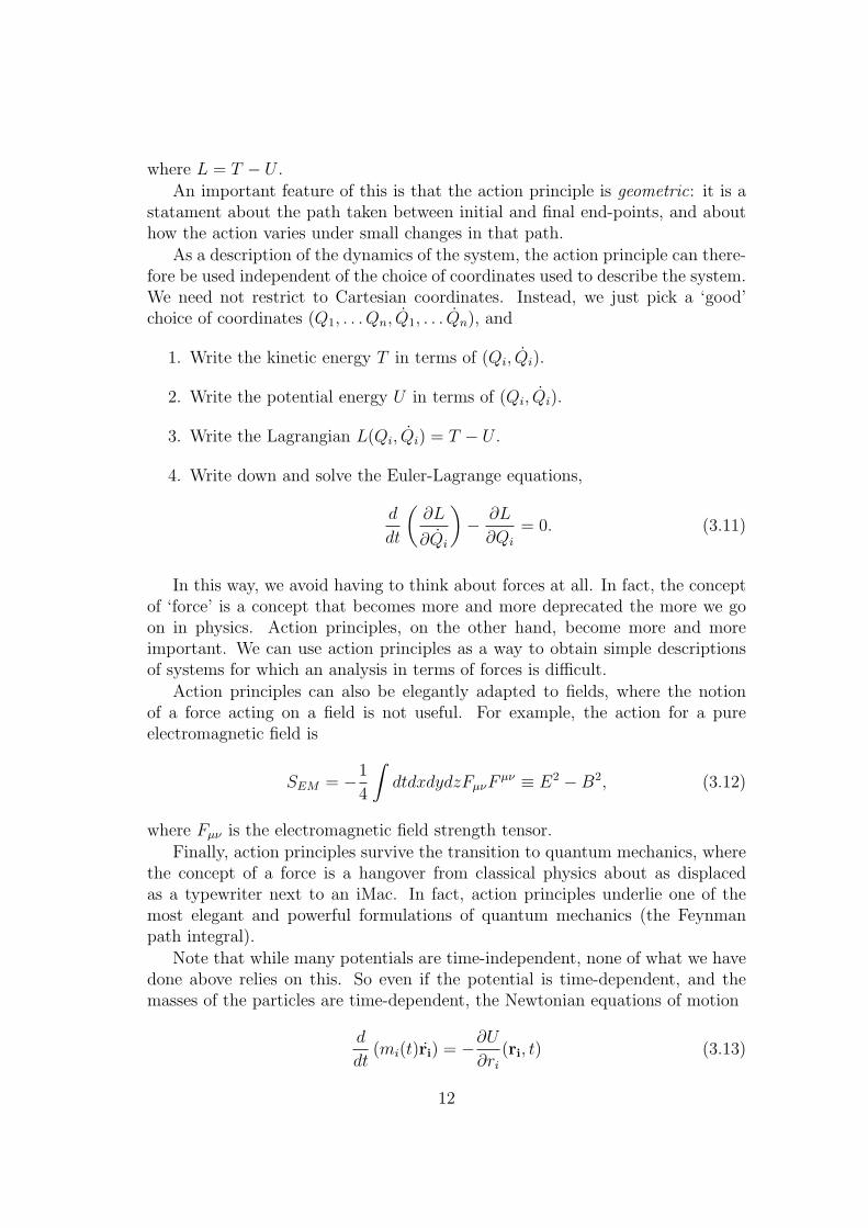
where L = T − U .An important feature of this is that the action principle is geometric: it is a
statament about the path taken between initial and final end-points, and abouthow the action varies under small changes in that path.
As a description of the dynamics of the system, the action principle can there-fore be used independent of the choice of coordinates used to describe the system.We need not restrict to Cartesian coordinates. Instead, we just pick a ‘good’choice of coordinates (Q1, . . . Qn, Q1, . . . Qn), and
1. Write the kinetic energy T in terms of (Qi, Qi).
2. Write the potential energy U in terms of (Qi, Qi).
3. Write the Lagrangian L(Qi, Qi) = T − U .
4. Write down and solve the Euler-Lagrange equations,
d
dt
(∂L
∂Qi
)− ∂L
∂Qi
= 0. (3.11)
In this way, we avoid having to think about forces at all. In fact, the conceptof ‘force’ is a concept that becomes more and more deprecated the more we goon in physics. Action principles, on the other hand, become more and moreimportant. We can use action principles as a way to obtain simple descriptionsof systems for which an analysis in terms of forces is difficult.
Action principles can also be elegantly adapted to fields, where the notionof a force acting on a field is not useful. For example, the action for a pureelectromagnetic field is
SEM = −1
4
∫dtdxdydzFµνF
µν ≡ E2 −B2, (3.12)
where Fµν is the electromagnetic field strength tensor.
Finally, action principles survive the transition to quantum mechanics, wherethe concept of a force is a hangover from classical physics about as displacedas a typewriter next to an iMac. In fact, action principles underlie one of themost elegant and powerful formulations of quantum mechanics (the Feynmanpath integral).
Note that while many potentials are time-independent, none of what we havedone above relies on this. So even if the potential is time-dependent, and themasses of the particles are time-dependent, the Newtonian equations of motion
d
dt(mi(t)ri) = −∂U
∂ri(ri, t) (3.13)
12
follow from the Lagrangian
L =∑i
1
2mi(t)ri
2 − U(ri, t) (3.14)
asd
dt
(∂L
∂ri
)=∂L
∂ri(3.15)
As we have said, Newton’s laws apply naturally in Cartesian coordinate systemsri, i = 1 . . . N . However we can use the action principle for any coordinate system
qj(ri), qj(ri, ri), ı, j = 1 . . . 3N.
There 3N corresponds to the fact that there are x, y, z coordinates for each par-ticle.
qi are then called generalised coordinates, and the qi are called generalisedvelocities. The 3N-dimensional space parametrised by the qi is called configurationspace. In analogy to dp
dt= F, we have
d
dt
(∂L
∂qi
)=∂L
∂qi. (3.16)
We therefore call pi =∂L∂qi
the generalised momentum and Fi =∂L∂qi
the generalisedforce.
There are two important conservation laws we can now derive. First, if theLagrangian does not depend on a coordinate, then the corresponding generalisedmomentum is conserved. Such a coordinate is called cyclic or ignorable. This
follows easily, as if ∂L∂qi
= 0, then ddt
(∂L∂qi
)= 0, and so pi =
∂L∂qi
is conserved.
An appropriate choice of generalised coordinates can make such conservationlaws obvious, and allows us to identify conserved quantities.
Example: motion in a spherical potential
Consider motion in a spherically symmetric potential V = V (r), where r =√x2 + y2 + z2. Then
T =1
2m(x2 + y2 + z2
), (3.17)
U = V (r). (3.18)
Let us transform to spherical polar coordinates. In these coordinates,
T =1
2m(r2 + r2θ2 + r2 sin2 θϕ2
), (3.19)
U = V (r). (3.20)
13

Therefore, as L = T − U ,
L = T − U =1
2m(r2 + r2θ2 + r2 sin2 θϕ2
)− V (r). (3.21)
The generalised momenta are
pr = mr, (3.22)
pθ = mr2θ, (3.23)
pϕ = mr2 sin2 θϕ. (3.24)
As ϕ does not appear explicitly in L, pϕ is a constant of motion and is thereforea conserved quantity.
In fact, as this system is spherically symmetric, we can go further. We canalways orient the sphere so that the initial conditions are θ = π/2, θ = 0. In thiscase, the equations of motion
d
dt(pθ) =
∂L
∂θ(3.25)
gived
dt
(mr2θ
)= mr2 sin θ cos θϕ2, (3.26)
and somr2θ = −2mrrθ +mr2 sin θ cos θϕ2 (3.27)
Initial conditions of sin θ = 0, θ = 0 then imply θ = 0. This implies that the initialconditions are then preserved, and so θ = π/2, θ = 0 remains true throughoutthe entire motion.
This shows that the motion of a particle under a radial force can be reduced toplanar motion, with pϕ = mr2ϕ a conserved quantity - this last quantity being ofcourse the angular momentum. This corresponds to the fact that motion under aradial potential can be reduced to motion in a plane: this should be familiar fromthinking about planetary orbits, where we can reduce a 3-dimensional problemto a 2-dimensional one.
Our intuition for mechanics tells us that there is normally another constantof the motion, the total energy.
Suppose the Lagrangian does not depend explicitly on time, and consider thefunction
H =∑i
q
(∂L
∂qi
)− L. (3.28)
(We will late introduce this as the Hamiltonian.)Suppose we have some function of the generalised coordinates and velocities,
f = f(qi, qi, t). Along a path of the system in configuration space, we have
df
dt=∑i
∂f
∂qi
dqidt
+∑i
∂f
∂qi
dqidt
+∂f
∂t. (3.29)
14

We therefore find that
d
dt
[∑i
q
(∂L
∂qi
)− L
]=
∑i
qi
(∂L
∂qi
)+∑i
qid
dt
(∂L
∂qi
)− dL
dt(3.30)
=∑i
qi
(∂L
∂qi
)+∑i
qid
dt
(∂L
∂qi
)−∑i
qi∂L
∂qi−∑i
qi
(∂L
∂qi
)=
∑i
qi
[d
dt
(∂L
∂qi
)− ∂L
∂qi
](3.31)
= 0, (3.32)
using the Euler-Lagrange equations. We therefore see that if the Lagrangian isindependent of time, then
H =∑i
qi
(∂L
∂qi
)− L (3.33)
is a constant of motion.
We can also check that if L = T−U , with U the potential energy independentof qi, and T a homogeneous function of degree 2 in qi (T =
∑ij cij qiqj), then∑
i
qi∂L
∂qi=∑i
qi∂T
∂qi= 2T. (3.34)
As a consequence,
H = (2T )− (T − U) = T + U. (3.35)
The conservation of H is therefore equivalent to the conservation of total energy.
The above results have all originated in familiar mechanical systems, but it isimportant to realise that they follow from more general principles.
1. The absence of a coordinate qi from the Lagrangian implies the conservationof the corresponding momentum ∂L
∂qi.
2. The independence of the Lagrangian on time t implies that the Hamiltonianis a constant of motion.
The relationship between spatiotemporal symmetries and conserved quantities isa deep one, which we shall further discuss in Noether’s theorem.
This relationship is also a relationship that extends to quantum mechanics,where you should make the connection with the fact that symmetries of theHamiltonian give rise to operators that commute with the Hamiltonian and arethus simultaneously diagonalisable.
15

3.2 Rotating Frames
One important and classic application of Lagrsngian mechanics is to describe themotion of a particle in a rotating frame of reference. Such a frame is not inertial,and so the coordinates used are rotating relative to those in an inertial frame.
Examples of rotating frames include
1. Coordinates fixed on a merry-go-round on a fair.
2. North-South-East-West coordinates on the earth, as the earth is rotatingdaily about its own axis.
Rotating frames are characterised by the existence of fictitious forces, of whichcentrifugal force is the best known example. We intend now to derive the formof, and equations for, these forces.
Let us start with the Lagrangian for particle motion in an inertial frame,
L = T − U =1
2mv2 − U. (3.36)
Now transform to a frame with the same origin as the inertial frame, but whichis rotating with respect to it with an angular velocity Ω.
Figure 3.1: Rotating about an axis with angular velocity Ω.
The velocities in the two frames are then related by
vinertial = vrotating +Ω× rrotating. (3.37)
This is an equation which is correct, but is easy to get confused by. So let usspend a little bit of time explaining this. First, it is a vector equation. It meansthat the velocity vector in the inertial frame is related to the velocity vector inthe rotating frame by an addition of a term Ω× rrotating. It states the identity ofthe two vectors. However, what it does not mean is that the x-component of thisvector using inertial frame x-coordinates is the same as the x-component of this
16

vector using rotating frame x-coordinates. That is, a vector V can be expandedas
V = Vi,rei,r = Vi,inertialei,inertial (3.38)
where ei,r are basis vectors for the rotating frame and ei,inertial are basis vectorsfor the inertial frames.
Returning to the main track, the significance of the action principle is that weknow we can obtain the equations of motion in the rotating frame by substitutingthe expression for vinertial into the expression for the Lagrangian.
We therefore have (the subscript r denotes ‘rotating frame’).
Lrotating =1
2m(vr +Ωr) · (vr +Ω× rr)− U (3.39)
=1
2mvr · vr +mv · (Ω× rr) +
1
2m(Ω× rr) · (Ω× rr)− U.(3.40)
We now evaluate the Euler-Lagrange equations for these coordinates
dLr = mvr · dvr +mdvr · (Ω× rr) +mvr · (Ω× drr)
+m (Ω× drr) · (Ω× rr)−∂U
∂rrdrr. (3.41)
We can use the vector triple product a · (b×c) = b · (c×a) = c · (a×b) to writethis as
dLr = mvr · dvr +mdvr · (Ω× rr) +mdrr · (vr ×Ω)
+mdrr · ((Ω× rr)×Ω)− ∂U
∂rr· drr. (3.42)
From this we can extract the derivatives
∂L
∂rr= m(vr ×Ω) +m ((Ω× rr)×Ω)− ∂U
∂rr, (3.43)
∂L
∂vr
= mvr +m(Ω× rr). (3.44)
The Euler-Lagrange equations ddt
(∂L∂vr
)− ∂L
∂rr= 0 then give︷ ︸︸ ︷
mdvr
dt+m
(Ω× rr
)+m (Ω× vr)
ddt(
∂L∂vr
)
=
−m(vr ×Ω)−m ((Ω× r)×Ω) +∂U
∂rr= 0. (3.45)
Rearranging this, we obtain
mdvr
dt= −∂U
∂rr+mrr × Ω+ 2mvr ×Ω+mΩ× (r×Ω). (3.46)
17

In addition to the ‘standard’ ∂U∂rr
force, there are three additional ‘fictitious’ forces.
The adjective ‘fictitious’ arises because these terms do not arise in inertial frames.1
1. mrr × Ω : this force depends on the non-uniformity of rotation.
2. 2mvr×Ω: this force is called the Coriolis force, and depends on the velocityof the particle.
3. mΩ× (r×Ω): this is the centrifugal force.
What is the physical origin of these forces? The first two follow from conservationof angular momentum.
For the first case, suppose you have a particle at fixed position rr in therotating frame. In the inertial frame, this therefore has a certain amount ofangular momentum as it rotates. Suppose we now increase the rotation rate ofthe rotating frame. If we keep the position rr fixed, then the angular momentumin the inertial frame will increase, and so to conserve angular momentum theparticle must experience a new ‘backwards’ force, which is rr × Ω.
rr
Figure 3.2: Particle at fixed position in a rotating frame.
The second case of the Coriolis force 2mvr × Ω is similar. If a particle hasa non-zero velocity in the rotating frame, then the effect of this is to change itsangular momentum in the inertial frame. The Coriolis force acts to counter this,ensuring that angular momentum is conserved in the inertial frame.
The final case of the centrifugal force mΩ × (r ×Ω) is similar. By thinkingin the inertial frame, it is clear that a particle with no forces on it will move ata constant velocity and thereby increase its radial separation from the origin. Ittherefore follows that in the rotating frame there should be a force which acts
1Note that under a more advanced understanding, the gravitational force is also a ‘fictitious’
force, arising because we do not use a frame moving along the geodesics of spacetime.
18

rv
Figure 3.3: Particle with fixed velocity in a rotating frame.
to increase the radial separation from the origin. This force is the centrifugalforce, with a constant tendency to expel bodies radially outwards in the planeperpendicular to the angular velocity vector.
vi
Figure 3.4: Particle with fixed velocity in an inertial frame.
Let us illustrate these fictitious forces with some examples.
1. A cylindrical glass beaker filled with liquid is rotated on a turntable at aconstant angular velocity ω. Find the equation of its surface.
We wait for the liquid to come to an equilibrium and go to coordinates thatare rotating with the turntable. The relevant force is then the centrifugalforce, as once everything has settled down there are no velocities withinthe rotating frame. In the rotating frame, the liquid is then subject to anadditional centrifugal force
F = mω2r (3.47)
19

directed radially outwards in cylindrical coordinates. We can regard thisforce as arising from a potential energy
U = −1
2mω2(x2 + y2). (3.48)
There is in addition the standard gravitational potential energy
V = mgz. (3.49)
We obtain the equation of the surface of the liquid from the equipotentialsurface, which is at
mgz − 1
2mω2(x2 + y2) = mgh0. (3.50)
Here the constant h0 is fixed as the height of the liquid at the centre of thebeaker.
2. (Foucault’s pendulum) For a plane pendulum, determine how the plane ofrotation changes due to the rotation of the earth.
This is a famous experiment that can be used to demonstrate the rotation ofthe earth. It involves a long pendulum that makes small angle oscillationsin the (x, y) plane, which are standard axes horizontal in the frame of thelaboratory. Naively one would think that the oscillation direction of thependulum would remain unchanged: if the pendulum is oscillating at anangle θ = tan−1(y/x) to the x-axis, it would continue to do so. The pointhowever is that, due to the rotation of the earth, the (x, y)-axes are notinertial. Instead they are actually a rotating frame, inherited from therotation of the earth.
The angular velocity vector of the earth points out of the north pole. Inthe above (x, y) coordinates, the z-axis points vertically out of the earth.The relevant component of the earth’s angular velocity vector is the partthat we resolve onto the z-axis (note that this component vanishes at theequator). This gives a Coriolis force within the (x, y) plane.
There is also a component of the earth’s angular velocity vector that points in the (x, y) plane. The
effect of the Coriolis force induced by this is vertical, and thus gives a tiny (and insignificant) change to
the effective value of g.
The overall effect of the Coriolis effect is to modify the equations of motionto
x+ ω2x = 2Ωzy, (3.51)
y + ω2y = −2Ωzx. (3.52)
20

z
Figure 3.5: Rotation with respect to the x-y plane.
We can solve this by writing z = x + iy. Multiplying equation (3.52) by iand combining, we get
(x+ iy) + ω2(x+ iy) = −2iΩz(x+ iy). (3.53)
We therefore havez + 2iΩz z + ω2z = 0. (3.54)
For the limit Ωz ≪ ω, this is solved by
z = exp(−iΩzt)[A1e
iωt + A2e−iωt]. (3.55)
The term exp(−iΩzt) corresponds to a slow rotation of the plane of oscil-lation.
For an angle Θ from the North Pole, then |Ωz| = ΩcosΘ, where Ω = 2π24 hours
.This rotation of the plane of oscillation then allows a direct demonstrationof the rotation of the earth.
3. A Fake Example A good story that you will read in several mechanicstextbooks involves the 1914 Battle of the Falkland Islands. Two Britishbattlecruisers headed down from the North Atlantic to engage a Germancruiser squadron; they subsequently caught and, after an extended battle,sunk them.2
According to the story, however, the British ships spent quite a while miss-ing early on in the battle. The reason? The guns were calibrated for theNorthern Hemisphere, where the Coriolis effect causes a systematic deflec-tion in one direction. In the Southern Hemisphere, the Coriolis effect acts
2The Germans had their revenge; one of the battlecruisers was later sunk at Jutland.
21

Figure 3.6: The angle with respect to the North Pole.
the other way, and so the guns were out by taking the wrong sign for theCoriolis effect.
However, while a nice story with correct physics, it is sadly an urban myththat has found its way into many textbooks.
4. Cyclones and hurricanes
Cyclones are caused by regions of low air pressure. This low pressure regioncauses air to flow in from the outer, high pressure regions. However the flowis not purely radial (as seen from above the earth), but instead modifies bythe Coriolis force into an angular flow that gives the characteristic spiralshapes of hurricanes as seen by satellites.
The direction of rotation is reversed in northern and southern hemispheres.As the angular velocity vector is inherited from the earth, in the northernhemisphere the angular velocity vector points out of the surface of the earth,and in the southern hemisphere the angular velocity vector points inwards,towards the centre of the earth. This reversal of the angular velocity vectorreverses the direction of the Coriolis force, and therefore cyclones rotateanticlockwise in the northern hemisphere and clockwise in the southernhemisphere.
3.3 Normal Modes
Our discussion of normal modes will be relatively brief as it is a topic that hasbeen treated previously in the first year classical mechanics course and also inthe dedicated first year Normal Modes and Waves course.
Suppose we have a mechanical system described by generalised coordinates(q1, . . . , qn) and a Lagrangian L(qi, qi) = T − U .
22
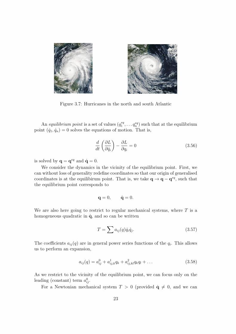
Figure 3.7: Hurricanes in the north and south Atlantic
An equilibrium point is a set of values (qeq1 , . . . qeqn ) such that at the equilibrium
point (q1, qn) = 0 solves the equations of motion. That is,
d
dt
(∂L
∂qi
)− ∂L
∂qi= 0 (3.56)
is solved by q = qeq and q = 0.
We consider the dynamics in the vicinity of the equilibrium point. First, wecan without loss of generality redefine coordinates so that our origin of generalisedcoordinates is at the equilibirum point. That is, we take q → q− qeq, such thatthe equilibrium point corresponds to
q = 0, q = 0.
We are also here going to restrict to regular mechanical systems, where T is ahomogeneous quadratic in q, and so can be written
T =∑
aij(q)qiqj. (3.57)
The coefficients aij(q) are in general power series functions of the qi. This allowsus to perform an expansion,
aij(q) = a0ij + a1ij,kqk + a2ij,klqkql + . . . (3.58)
As we restrict to the vicinity of the equilibrium point, we can focus only on theleading (constant) term a0ij.
For a Newtonian mechanical system T > 0 (provided q = 0, and we can
23
diagonalise, rotating coordinates so that we have
T = ( q1 q2 . . . qn ) (D)
q1
q2
. . .
qn
(3.59)
with D a diagonal matrix. In terms of the new q′coordinates, we can then write
T =1
2
∑i
q′,2i (3.60)
U = U(q′). (3.61)
Again, by expanding U(q′) about q′= 0, we can extract the quadratic terms as
the leading non-constant contribution of the potential energy.
U = U0 +∑i,j
1
2Uijq
′
iq′
j. (3.62)
Note that all the linear terms vanish as q′= 0 is an equilibrium point. The
equations of motion then become
q′= Uq
′. (3.63)
We have neglected here any higher order terms. This neglect is a good approxi-mation sufficiently close to the equilibrium point. What is meant by ‘sufficiently’close will vary from example to example depending on the numerical factors.However the beauty of an equilibrium point is that we can always find valuesthat are ‘sufficiently’ close.
The equations are now standard second order differential equations which wecan solve using very standard techniques. We solve these equations by findingthe eigenvalues and eigenvectors of U. The eigenvectors give the normal modes.These are the directions in coordinate space away from the equilibrium pointalong which small oscillations behave as a linear simple harmonic oscillator: θ =(±)λ2θ.
The signs of the eigenvalues determine whether the mode is stable or unstable.If all eigenvalues are negative (θ = −λ2θ in all directions), then the equilibriumpoint is stable.
Otherwise, the equilibrium point is unstable (as it only takes a single unstabledirection to make the entire equilibrium point unstable).
Expanding general mechanical systems about their equilibrium points anddetermining the normal modes allows the stability of a system to be determined.
24

3.4 Particle in an Electromagnetic Field
One way to approach mechanics is to take the action principle as axiomatic. Wewrite down different Lagrangians, and derive the different equations of motionthat follow from these Lagrangians and compare with experiment. In this waywe do not ask ‘What forces act on a particle?’ but instead ’What Lagrangiandescribes the system?’
This approach is actually the most fruitful in terms of understanding moreadvanced physical systems. Lagrangians remain useful long after forces disappear.
In this vein, let us consider the Lagrangian
L =1
2mr2 + qr ·A(r, r)− qϕ(r, t), (3.64)
where r is the ordinary (x, y, z) position vector for a particle. At the level ofwriting this Lagrangian down, ϕ(r, t) and A(r, t) are just background scalar andvector functions of r. We will subsequently interpret these as the scalar andvector potentials of electromagnetism, but to start with these are just arbitraryfunctions.
Note also that if we regard the Lagrangian approach as fundamental, then eq.(3.64) is something completely natural to write down. We have simply extendedour previous Lagrangians, which had terms quadratic in r and terms with nodependence on r, to include a term that is linear in r. From this perspective,eq. (3.64) is the simplest possible way to extend the Lagrangians previouslyconsidered.
From this Lagrangian, we can then derive
px =∂L
∂x= mx+ qAx, (3.65)
and generallyp = mr+ qA. (3.66)
The equations of motion for this Lagrangian are
d
dt
(∂L
∂r
)− ∂L
∂r= 0 (3.67)
and so
d
dt(mx+ qAx) = q (x∂xAx(r, t) + y∂xAy(r, t) + z∂xAz(r, t)− q∂xϕ)(r, t))
(3.68)where we have written out the equations of motion for the x-coordinate. Now,
dAx(r, t)
dt=∂Ax(r, t)
∂t+ x∂xAx(r, t) + y∂yAx(r, t) + z∂zAx(r, t) (3.69)
25

and so we have
mx+ q∂Ax(r, t)
∂t+ qx∂xAx(r, t) + qy∂yAx(r, t) + qz∂zAx(r, t)
= q (x∂xAx(r, t) + y∂xAy(r, t) + z∂xAz(r, t))− q∂xϕ(r, t).
Cancelling terms and rearranging, this gives the equation of motions
mx = q
(−∂xϕ(r, t)−
∂Ax(r, t)
∂t
)+qy (∂xAy − ∂yAx) + qz (∂xAz − ∂zAx) . (3.70)
Now, we recall from electromagnetism that the E and B fields are related to thescalar potential ϕ(r, t) and the vector potential A(r, t) by
E = −∇ϕ− ∂A
∂t, (3.71)
B = ∇×A. (3.72)
and so we havemx = qEx + q (yBz − zBy) , (3.73)
givingmx = q (Ex + (v ×B)x) (3.74)
Generalising now to the equations of motion for all coordinates, we see that theparticle Lagrangian
L =1
2mr2 + qr ·A(r, r)− qϕ(r, t), (3.75)
gives equations of motion
mr = q (E+ (v ×B)) , (3.76)
which is precisely the Lorenz force law. This Lagrangian therefore gives theequations of motion for, and this describes, the motion of a particle in an externalelectromagnetic field.
Let us make some general comments on this.
1. The Lagrangian cannot be written as T − U : the ‘potential energy’ termhas a linear factor of r, and so the T − U structure is not valid here.
2. Note that the coupling
q
∫dt r ·A(r, t)− ϕ(r, t) (3.77)
26

is already relativistic. If we consider 4-vectors, we have
dt (r, 1) = dt
(dr
dt,dt
dt
)= dt
(dτ
dt
dr
dτ,dτ
dt
dt
dτ
)(3.78)
= dτ
(dr
dτ,dt
dτ
)= dτUµ, (3.79)
where Uµ is the 4-velocity. We therefore see that we can write this couplingin the manifestly relativistic form,∫
dtr ·A(r, t)− ϕ(r, t) =
∫dτUµAµ (3.80)
with Aµ = (ϕ,A) the 4-potential.
3. Note that this Lagrangian gives the dynamics of a particle coupled to abackground electromagnetic field. It does not give the dynamics of theelectromagnetic field itself. This is given by
S =1
4
∫d4xFµνF
µν (3.81)
=1
2
∫d4x
(E2 −B2
). (3.82)
Here Fµnu = ∂µAν − ∂νAµ is the electromagnetic field strength tensor.
4. The Lagrangian formulation allows us to easily work out the dynamics of aparticle coupled to electromagnetism in more general coordinate systems.We simply re-express the Lagrangian in the new coordinates, and thenevaluate the Euler-Lagrange equations.
3.5 Rigid Bodies
We next want to consider the dynamics of a rigid body. A rigid body is a systemof very many particles where the distances between each pair of particles do notvary. This is an idealisation, but one that serves to capture many real systems.
A little bit of thought should be sufficient to convince oneself that rigid bodiesare described by six degrees of freedom. These correspond to
• three position coordinates
• three angular coordinates: two to choose an axis, and one to rotate aboutthat axis.
27

This is one of these results that is best proved by thinking about it until youconvince yourself that it is correct.
For regular Newtonian mechanical systems, the dynamics of a rigid body canbe described by the standard Lagrangian,
L = T − U. (3.83)
In working with rigid bodies, our first goal is to find an expression for T for arigid body that is both moving translationally and also rotating about its ownaxis. Now,
T =∑i
1
2miv
2, (3.84)
where the sum over i is a sum over all possible constituent elements of the rigidbody. Now if the body has centre of mass velocity V, and ri is the displacementvector of the element i from the centre of mass, then
vi = Vi +Ω× ri, (3.85)
as per our previous calculations for the case of rotating frames. We can expandthis to give
T =∑i
1
2mi (V ·V + 2V · (Ω× ri) + (Ω× ri) · (Ω× ri)) . (3.86)
Now,
V · (Ω×∑i
miri) =∑i
miri · (V ×Ω)
and∑miri = 0, as ri is the displacement vector from the centre of mass, and by
definition of the centre of mass∑miri = 0. We also have
(Ω× ri) · (Ω× ri) = ϵαβγΩα(ri)βϵγδϵΩδ(ri)ϵ
= (δαδδβϵδαϵδβδ) Ωα(ri)βΩδ(ri)ϵ
= ΩαΩδ
(δαδ(ri)
2 − (ri)α(ri)δ). (3.87)
We can therefore write
T =1
2MV ·V +
1
2ΩαΩδ
(∑i
mi(δαδ(ri)2 − (ri)α(ri)δ)
)︸ ︷︷ ︸
Iαδ
. (3.88)
Here Iαδ is called the inertia tensor and can be directly evaluated for any givenshape of a rigid body.3 We can then write
T =1
2MV ·V︸ ︷︷ ︸
LinearKEof CoM
+1
2IαδΩαΩδ︸ ︷︷ ︸
RotationalKEaboutCoM
, (3.89)
3If you are frightened by the name ‘tensor’, you might like to call this the inertia matrix
instead. It will be equivalent for all purposes here.
28

and also
L = T − U =1
2MV ·V +
1
2IαδΩαΩδ︸ ︷︷ ︸
function of generalised velocities
−U. (3.90)
The inertia tensor Iαδ is a symmetric tensor. In the above equation, Ωα gives theangular velocities about (x, y, z) coordinate axes. We can obtain the correspond-ing angular momentum,
Lα =∂L
∂Ωα
= IαδΩδ. (3.91)
You can check that this is equivalent to the more conventional definition of L =∑imiri × vi.
The relationship between L and Ω in equation (3.91) shows that the angularmomentum vector Lα is not in general parallel to the angular velocity vector Ωα,except in the case that Ωα lies along one of the eigenvectors of the inertia tensorI. The eigenvectors of I are called the principal axes :
IΩ = λΩ, (3.92)
with three eigenvalues denoted by I1, I2, I3. There are three cases:
I1 = I2 = I3 : the asymmetric top (3.93)
I1 = I2 = I3 : the symmetric top (3.94)
I1 = I2 = I3 : the spherical top (3.95)
The equations of motion for a rigid body are then found as the Euler-Lagrangeequations for
L =1
2MV ·V +
1
2IαδΩαΩδ︸ ︷︷ ︸
function of generalised velocities
−U, (3.96)
in terms of the six generalised coordinates (three translational and three rota-tional) that are required to specify the state of the system.
Some ways of choosing generalised coordinates are more equal than others.For problems of rotating bodies, a standard choice are the so-called Euler angles.However we will not go into detail here.
In certain cases of rigid bodies, there may also be constraint equations. Forexample, when a rigid body rolls on a rough surface, the velocity at the pointof contact with the ground is required to vanish. This gives rise to constraintequations of the form ∑
i
Cαi(q)qi = 0. (3.97)
These constraints fall into two kinds.
29
1. Holonomic constraints, where the constrain can be integrated so as to reducesolely to a relationship between coordinates.
An example is a cylinder rolling on a rough plane, where the translationalcoordinate x and the rotational coordinate θ are related by
x = Rθ, (3.98)
and so we can integrate this to x = Rθ + c.
2. Non-holonomic constraints, which are not integrable.
The classic example of this is a sphere rolling on a rough plane. In this casethe extra degrees of freedom of the sphere means that it is not possible tointegrate the constraint equation: the addition of the axis of rotation of thesphere about its pole means that we cannot use the fact that the velocityof the sphere at the point of contact with the ground vanishes to derive arelationship between coordinates.
For non-holonomic constraints, we have to include the constraint explicitlyin the extremisation procedure through use of a Lagrange multiplier.
3.6 Noether’s Theorem
To conclude our discussion of Lagrangian mechanics, we now discuss Noether’stheorem. This is a general theorem relating symmetries of the Lagrangian toconserved quantities.
Suppose we have a continuous set of coordinate transformations parametrisedby a continuous parameter s,
Ts : qi → Qi(s), with Qi(0) = qi,
such thatL(qi(t), qi(t), t) = L(Qi(s, t), Qi(s, t), t). (3.99)
These transformation are then a map of coordinate space onto coordinate space.This map then also induces a map on velocity vectors as well.4 The map onvelocity vectors should be intuitive: as you map coordinates to coordinates, youmap old trajectories to new trajectories, and thus you can evaluate the velocityvectors of the new trajectories at each point. This defines the map from oldvelocities to new velocities.
The information content lies in the statement that under this map the valueof the Lagrangian at each point is the same, and thus we say that this map is
4In mathematics texts, you will see this stated in the form that a map on a manifoldM → M
induces a map on the tangent bundle, TM → TM .
30

a symmetry of the Lagrangian. To keep out intuition in order, it is helpful tokeep in mind that the simplest examples of such transformations are rotations ortranslations.
The fact that L is, by construction, invariant under these transformationstells us that
d
ds
[L(Qi(s, t), Qi(s, t), t)
]= 0, (3.100)
and so by the chain rule ∑i
∂L
∂Qi
dQi
ds+
∂L
∂Qi
dQi
ds= 0. (3.101)
Now, as the coordinate mapping preserves the Lagrangian, it will also take so-lutions of Lagrange’s equations to solutions of Lagrange’s equations. (We cansee this by thinking about the action principle; as the action for any path isunchanged, extremals of the action remain extremals of the action) Therefore,
∂L
∂Qi
=d
dt
(∂L
∂Qi
),
and so we get ∑i
d
dt
(∂L
∂Qi
)∂Qi
∂s+
∂L
∂Qi
d
ds
(∂Qi
dt
)= 0 (3.102)
and therefored
dt
[∑i
(∂L
∂Qi
)dQi
ds
]= 0. (3.103)
This is true for all s. However it is useful to evaluate this at the value s = 0corresponding to the original coordinates. We then get
d
dt
[∑i
pidQi
ds|s=0
]= 0. (3.104)
The reason for evaluating these at s = 0 is that this is the point in which co-ordinate space we imagine examining the evolution of the system. We thereforeobtain Noether’s theorem:
If a continuous coordinate mapping qi → Qi(s, t), s ∈ R, preserves the La-grangian:
L(qi(t), qi(t), t) = L(Qi(s, t), Qi(s, t), t)
then ∑i
pidQi
ds|s=0
is a constant of the motion.
31

Noether’s theorem gives the general version of the statement that linear mo-mentum is conserved as a consequence of translational invariance, and angularmomentum is conserved as a consequence of rotational invariance.
It makes the deep connection between space-time symmetries and conservedquantities: this is a connection that holds for both classical and quantum me-chanics.
32

Chapter 4
Hamiltonian Mechanics
4.1 Hamilton’s Equations
We now introduce a new approach to classical mechanics. Whereas Lagrangianmechanics tends to be more useful for solving practical calculational problems,Hamiltonian mechanics allows more of the global structure and conceptual prop-erties of classical mechanics to be understood. It is also the approach to mechanicsthat transitions naturally to the canonical approach to quantum mechanics.
In Lagrangian mechanics a system is described as a motion through (qi, qi)space as a function of t, and the state of the system is viewed as set by the valuefor (qi, qi) at any one time.
The essence of Hamiltonian mechanics is to choose new coordinates (qi, pi)on this space. These coordinates are an equally good description as the orig-inal (qi, qi) coordinates: one can move freely back and forth between the twodescriptions. The coordinates are
(qi, pi) ≡(qi,
∂L
∂qi
). (4.1)
Here pi = pi(qi, qi) and qi = qi(qi, pi).To get the equations of motion, note that along a trajectory of the motion
dL =∑i
∂L
∂qidqi +
∑i
∂L
∂qidqi +
∂L
∂tdt
=∑
pidqi +∑
pidqi +∂L
∂tdt
=∑
pidqi + d(∑
piqi
)=∑
qidpi +∂L
∂t. (4.2)
Now we have
d (piqi − L) =∑
qidpi −∑
pidqi −∂L
∂t. (4.3)
33

We can then define a quantity
H(qi, pi, t) =∑
piqi − L, (4.4)
so
dH =∑
qidpi −∑
pidqi −∂L
∂tdt (4.5)
along trajectories of the motion. In terms of H(qi, pi), the equations of motionare then
qi =∂H
∂pi, (4.6)
pi = −∂H∂qi
. (4.7)
These equations are called Hamilton’s equations or less commonly the canonicalequations. Written in this form, the equations of motion are far more symmetricalthan in the treatment of Lagrangian mechanics.
Let us make some comments on this.
1. Although we write H(qi, pi) =∑piqi − L, we must read this as
H(qi, pi) =∑
piqi(qi, pi)− L(qi, pi). (4.8)
That is, H is a function of qi and pi alone, and any explicit appearance ofqi must be eliminated in favour of qi and pi.
2. The coordinate space (qi, pi) described by (q, p) coordinates is often denotedas phase space.
3. For qi = qi(qi, pi) to be well defined, we need ∂2L∂qi∂qj
to be positive definite.
In practice, this does not tend to be an issue.
4. We also see that (∂H
∂t
)q,p
= −(∂L
∂t
)q,q
. (4.9)
Let us give some examples of Hamiltonians.
1. A particle moving in a plane described by Cartesian coordinates has
L =1
2m(x2 + y2
)− U(x, y). (4.10)
andpx = mx, py = my.
The Hamiltonian is then
H =p2x2m
+p2y2m
+ U(x, y). (4.11)
34

2. A particle in a plane in plane polars,
L =1
2m(r2 + r2ϕ2
)− U(r, ϕ), (4.12)
haspr = mr, pϕ = mr2ϕ.
The Hamiltonian is
H =p2r2m
+p2ϕ
2mr2+ U(r, ϕ). (4.13)
3. A particle in an electromagnetic field has
L =1
2mx2 + q (x ·A− ϕ) . (4.14)
It then hasp = mx+ qA. (4.15)
The Hamiltonian is
H = p · x− L
= mx2 + qA · x− qx ·A+ qϕ
=(p− qA)2
2m+ qϕ. (4.16)
4.2 Hamilton’s Equations from the Action Prin-
ciple
We here provide a brief standalone derivation of Hamilton’s equations directlyfrom the action principle. We can write the action as
S =
∫Ldt =
∫ ∑pidqi −Hdt, (4.17)
where we have used the relationship L =∑piqi − H. Instead of extremising
through independent variations with respect to q and q, we now extremise treatingqi and pi as the independent variables, although for simplicity we present theargument where there is just a single conjugate (q, p) pair. Then
δS =
∫δpdq + pd(δq)−
(∂H
∂qδq
)dt−
(∂H
∂p
)δpdt
= =
∫δp
(dq −
(∂H
∂p
)dt
)+ δq
(−dp− ∂H
∂qdt
)+ d (pδq) . (4.18)
35

As∫d [pδq] = 0 as the δq variations are constrained to vanish at the endpoints,
we directly recover Hamilton’s equations,
q =∂H
∂p, (4.19)
p = −∂H∂q
. (4.20)
4.3 Poisson Brackets
We now want to introduce a topic that should help make the map from Hamilto-nian mechanics to quantum mechanics clear. Indeed, we will make the equationsof classical mechanics look almost the same as the equations of quantum mechan-ics!
Let f = f(q,p, t) be some general function on phase space. Then along thetrajectories of motion,
df
dt=
∑i
∂f
∂qi
dqidt
+∂f
∂pi
dpidt
+∂f
∂t
=∑i
(∂f
∂qi
∂H
∂pi− ∂f
∂pi
∂H
∂qi
)+∂f
∂t. (4.21)
We define the quantity
[H, f ] =∑i
(∂H
∂qi
∂f
∂pi− ∂H
∂pi
∂f
∂qi
), (4.22)
as the Poisson bracket of H and f (NB: the sign (which is entirely a matter ofconvention) has been reversed as to the presentation in the lectures). Generally,we define the Poisson bracket of f and g as
[f, g] =∑i
(∂f
∂qi
∂g
∂pi− ∂f
∂pi
∂g
∂qi
). (4.23)
Note [f, g] = − [g, f ]. If f is not an explicit function of t, we then have
df
dt= [f,H] . (4.24)
and therefore f is a conserved quantity if the Poisson bracket ofH and f vanishes.This should ring bells with your knowledge of quantum mechanics, where
conserved quantities in quantum mechanics are those which commute with theHamiltonian, and also with Ehrenfest’s theorem:
d
dt⟨O⟩ = ⟨[O,H]⟩+ ⟨∂O
∂t⟩, (4.25)
36

where these are now the commutators of quantum mechanics.Let us enumerate some properties of Poisson brackets:
[f, g] = − [g, f ] , (4.26)
[f1 + f2, g] = [f1, g] + [f2, g] , (4.27)
[f1f2, g] = f1 [f2, g] + f2 [f1, g] , (4.28)
∂
∂t[f, g] =
[∂f
∂t, g
]+
[f,∂g
∂t
]. (4.29)
Also note that
[qk, f ] =∂f
∂pk, (4.30)
[pk, f ] =∂f
∂qk. (4.31)
We therefore have
[qi, qj] = [pi, pj] = 0, (4.32)
[qi, pj] = δij, (4.33)
relationships which should look very familiar from quantum mechanics. It canalso be shown that (the proof is not difficult, just a little fiddly)
[f, [g, h]] + [g, [h, f ]] + [h, [f, g]] = 0. (4.34)
This relationship is called Jacobi’s identity.If it is not already blindingly obvious, then let us state explicitly that in
Poisson brackets you see the classical precursors of the commutators of quantummechanics.
Poisson brackets play an important role in constructing conserved quantitiesin Hamiltonian mechanics. Suppose f and g are constants of the motion, so
df
dt= [f,H] +
∂f
∂t= 0, (4.35)
dg
dt= [g,H] +
∂g
∂t= 0. (4.36)
Then [f, g] is also a conserved quantity. To prove this, note that
d
dt[f, g] = [[f, g] , H] +
∂
∂t[f, g] . (4.37)
From the Jacobi identity,
[[f, g] , H] = [f, [g,H]] + [g, [H, f ]] , (4.38)
37
and from the general properties of Poisson brackets ∂∂t[f, g] =
[∂f∂t, g]+[f, ∂g
∂t
].
It then follows that
d
dt[f, g] =
[∂f
∂t, g
]+
[f,∂g
∂t
]+ [f, [g,H]] + [g, [H, f ]]
=
[∂f
∂t− [H, f ] , g
]+
[f,∂g
∂t− [H, g]
]=
[df
dt, g
]+
[f,dg
dt
](4.39)
= 0, (4.40)
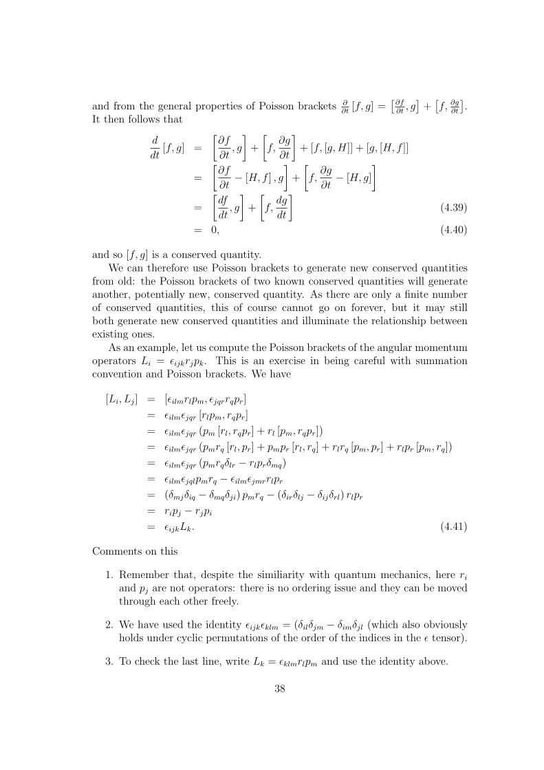
and so [f, g] is a conserved quantity.We can therefore use Poisson brackets to generate new conserved quantities
from old: the Poisson brackets of two known conserved quantities will generateanother, potentially new, conserved quantity. As there are only a finite numberof conserved quantities, this of course cannot go on forever, but it may stillboth generate new conserved quantities and illuminate the relationship betweenexisting ones.
As an example, let us compute the Poisson brackets of the angular momentumoperators Li = ϵijkrjpk. This is an exercise in being careful with summationconvention and Poisson brackets. We have
[Li, Lj] = [ϵilmrlpm, ϵjqrrqpr]
= ϵilmϵjqr [rlpm, rqpr]
= ϵilmϵjqr (pm [rl, rqpr] + rl [pm, rqpr])
= ϵilmϵjqr (pmrq [rl, pr] + pmpr [rl, rq] + rlrq [pm, pr] + rlpr [pm, rq])
= ϵilmϵjqr (pmrqδlr − rlprδmq)
= ϵilmϵjqlpmrq − ϵilmϵjmrrlpr
= (δmjδiq − δmqδji) pmrq − (δirδlj − δijδrl) rlpr
= ripj − rjpi
= ϵijkLk. (4.41)
Comments on this
1. Remember that, despite the similiarity with quantum mechanics, here riand pj are not operators: there is no ordering issue and they can be movedthrough each other freely.
2. We have used the identity ϵijkϵklm = (δilδjm − δimδjl (which also obviouslyholds under cyclic permutations of the order of the indices in the ϵ tensor).
3. To check the last line, write Lk = ϵklmrlpm and use the identity above.
38

4. This relation should look very similar to the quantum mechanical angularmomentum commutation relations, e.g. [Lx, Ly] = i~Lz.
We therefore see that the algebra of Poisson brackets is thus also very similar tothe algebra of quantum mechanical operators.
4.4 Liouville’s Theorem
We now want to describe another aspect of Hamiltonian mechanics, which givesthe closest classical version of the uncertainty principle (lots of quantum me-chanics has classical avatars - quantum mechanics was revolutionary, but not astotally revolutionary as it might first appear).
As we have said, Hamiltonian mechanics describes systems as trajectories(qi(t), pi(t)) in phase space. This we can view as a flow in phase space, analogousto the flow of a fluid. Now suppose we have a certain volume in phase space.
q
p
i
i
Figure 4.1: Flow in phase space
This volume we view in the same way as we view a volume of fluid that movesalong with the flow of the fluid: it is enclosed by a surface, and as the surface iscarried along by the flow then the volume enclosed is also carried along the flow.
We consider the flow of this volume(defined as the volume enclosed by theboundary surface as it moves along under Hamilton’s equations). Liouville’stheorem is the statement that
Volume in phase space is conserved during the motion of a Hamiltonian sys-tem.
To prove this, let us think about how the volume changes under a motion.We let S be the surface enclosing the volume. Near any element of hypersurface
39

q
p
i
i
Figure 4.2: Flow of a volume in phase space
dS, with a normal vector n,the instantaneous change in volume is
dV = v · ndS (4.42)
where v is the velocity vector of the flow at that point on the surface. This iseasiest to visualise for 3-dimensions, but a little thought should convince you thatit holds for an arbitrary number of dimensions.
The change in the overall volume along the flow is then
dV
dt=
∫S
v · ndS. (4.43)
By Gauss’s law (the divergence theorem), which holds for higher dimensions inexactly the same way as it holds for three dimensions, this can be rewritten as
dV
dt=
∫S
v · ndS =
∫V
∇ · vdV. (4.44)
Expressed in terms of coordinates (qi, pi), however,
∇ · v =
(∂
∂qi,∂
∂pi
)· (qi, pi)
=∂
∂qi(qi) +
∂
∂pi(pi)
=∑i
∂
∂qi
(∂H
∂pi
)− ∂
∂pi
(∂H
∂qi
)= 0. (4.45)
It therefore follows thatdV
dt= 0, (4.46)
40

and volume in phase space does not change under a Hamiltonian flow.Why is Liouville’s theorem the classical equivalent of the uncertainty prin-
ciple? Let us focus on a simple mechanical system with a single pair of (Q,P )coordinates (no index).
For simplicity we are going to focus on rectangular distributions. Suppose weinitially know that a system has |Q − Q0| < ∆Q0 and |P − P0| < ∆P0, and wethen allow it to evolve under a Hamiltonian flow. As volume in phase space isconserved, there is no way it can evolve to allow us arbitrarily good knowledgeof both Q and P .
In fact, the better our subsequent knowledge of Q, the worse our subsequentknowledge of P and vice-versa. If we stick for simplicity with rectangular distri-butions, then if at a time tf , |Q−Qf | < ϵ∆Q0, the constraint on P can only be|P − Pf | < ∆P0
ϵ, as volume in phase space is conserved.
q
p
i
i
P
Q
0
0
Figure 4.3: Initial ‘uncertainty’ in phase space
q
p
i
i
P
Q
f
f
Figure 4.4: Final ‘uncertainty’ in phase space
Note that Liouville’s theorem is a however a theorem about the total volume
41

of phase space. It is not a theorem about the individual pairs of conjugate coor-dinates. There are (more advanced) results involving these pairs of coordinates- these results involve what are called the Poincare integral invariants. Howeverthat is beyond the scope of this course.
Note also that Liouville’s theorem holds for any set of variables (Qi, Pi) suchthat
Qi =∂H
∂Pi
, Qi = − ∂H
∂Qi
. (4.47)
It therefore applies for all variables that are related by the canonical transforma-tions we are about to discuss.
4.5 Canonical Transformations
We have seen how to get Hamilton’s equations,
qi =∂H
∂pi, (4.48)
pi = −∂H∂qi
. (4.49)
So far, we have regarded the coordinates qi as originating as spatial coordinates,with pi their conjugate momenta. However we now want to think of more generalcoordinate transformations on phase space,
(qi, pi) → (Qi(qi, pi), Pi(qi, pi)) , (4.50)
which preserve Hamilton’s equations: we want the transformation to be such thatthe equations of motion for (Qi, Pi) are
Qi =∂H
′
∂Pi
, (4.51)
Pi =∂H
′
∂Qi
. (4.52)
for some Hamiltonian H′(Qi, Pi). This implies that (Qi, Pi), as coordinates on
phase space, retain the Hamiltonian structure. It is not true that general co-ordinate choices on phase space will keep the Hamiltonian structure - so this isrestricting to special possible choices of coordinates.
Note that under such a transformation, Qi is no longer necessarily a spatialcoordinate: (Qi, Pi) are now just some pair of coordinates on phase space thatretain the Hamiltonian structure, and Qi need no longer have an interpretationas a spatial coordinate.
42

Example: A very simple example of a canonical transformation is
Qi = −pi, Pi = qi, H′= H. (4.53)
This simply exchanges position and momentum coordinates, and it is easy to seethat the new coordinates also obey Hamilton’s equations.
What are the general conditions for a canonical transformation? We define atransformation to be canonical if[∑
k
PkdQk −H′(Qk, Pk, t)dt
]−
[∑k
pkdqk −H(qk, pk, t)dt
]= dG, (4.54)
where G is some function on phase space.To see this, recall that as H =
∑k pkqk − L, L =
∑pkqk − H. It therefore
follows that ∫ tf
ti
Ldt =
∫ ∑k
pkdqk −H′dt. (4.55)
If the above equation holds, we then have∫ (qf ,tf )
(qi,ti)
Ldt =
∫ (qf ,tf )
(qi,ti)
[∑k
PkdQk −H′dt
]− dG, (4.56)
and so
G(qf )−G(qi) +
∫ (qf ,tf )
(qi,ti)
Ldt =
∫ (qf ,tf )
(qi,ti)
[∑k
PkdQk −H′dt
]. (4.57)
We therefore see that extremisation of∫Ldt carries the same information as
extremisation of∫L
′dt =
∫ ∑k PkdQk−H
′dt, as the G total derivative drops out.
It therefore also follows that the (Q,P ) coordinates obey Hamilton’s equations,
Qi =∂H
′
∂Pi
, (4.58)
Pi = −∂H′
∂Qi
, (4.59)
and so (Qi, Pi) do indeed represent a set of canonical coordinates.Let us make a side comment. As the extermisation of
∫Ldt and
∫λLdt, for λ a constant, give the same
result, we could have instead considered
λ
[∑k
PkdQk −H′(Qk, Pk, t)dt
]−
[∑k
pkdqk −H(qk, pk, t)dt
]= dG, (4.60)
and we would also have found that (Q,P ) obey Hamilton’s equations. By convention, only the case with λ = 1
is called a canonical transformation (λ = 1 is called an extended canonical transformation).
We can construct canonical transformations (implicitly) through the choiceof a generating function G. The different possibilities are when the function Gdepends on
43
1. Old and new coordinates G(q,Q) - ‘type 1 generating function’
2. Old coordinates and new momenta G(q, P ) - ‘type 2 generating function’
3. New coordinates and old momenta G(Q, p) - ‘type 3 generating function’
4. Old and new momenta G(p, P ) - ‘type 4 generating function’
We first consider the case where the generating function is G1(q,Q). It thenfollows that
dG =∂G1
∂tdt+
∂G1
∂qdq+
∂G1
∂QdQ. (4.61)
We then have∑PkdQk −H
′(Qk, Pk, t)dt =
(−H(qk, pk, t) +
∂G1
∂t
)dt (4.62)
+∑k
(pk +
∂G1
∂qk
)dqk +
∑k
∂G
∂Qk
dQk.
As we can vary q and Q independently, we then have
∂G
∂qk= −pk, (4.63)
∂G
∂Qk
= Pk, (4.64)
H′
= H − ∂G1
∂t. (4.65)
These equations give, implicitly, the relationship between the coordinates (q,p)and the coordinates (Q,P).
This all sounds a bit abstract, and so let us illustrate with an example. Wetake a simple case: G = q ·Q. Then these equations give
p = −Q,q = P, H′= H. (4.66)
This is the same example as we saw earlier.We now consider the second type of canonical transformation. Here we gen-
erally write G = Q ·P +G2(q,P, t). (The use of the additional Q ·P is to givea convenient set of equations below)
We then have∑k
PkdQk −H′(Qk, Pk, t)dt =
(−H(qk, pk, t) +
∂G2
∂t
)dt+
∑k
PkdQk +QkdPk
+∑k
(pk +
∂G2
∂qk
)dqk +
∑k
∂G2
∂Pk
dPk. (4.67)
44

In this case we get the implicit equations
∂G2
∂qk= −pk,
∂G2
∂Pk
= −Qk, H = H′+∂G2
∂t. (4.68)
Again, we must solve these equations implicitly to obtain the coordinate trans-formation
Canonical transformations are general transformations on phase space. Theyare therefore rather far removed from the direct positional interpretation of co-ordinates. They are useful for revealing the general structure of mechanics, butwe have now moved away from pendula hanging from rotating tops.
Note that with the canonical transformation of the second kind, it is easy forus to recover the identity transformation. If we take
G = Q ·P− q ·P (4.69)
(i.e. G2 = −q ·P), then we have from
∂G2
∂qk= −pk,
∂G2
∂Pk
= −Qk, H = H′+∂G2
∂t. (4.70)
the relations Pk = pk, Qk = qk. We have therefore recovered the identity trans-formation. We could therefore construct infinitesimal canonical transformationsby starting with the above transformation, and considering infinitesimal modifi-cations to it.
We now want to analyse the behaviour of Poisson brackets under canonicaltransformations. We are going to restrict here to time-independent transforma-tions, where the function G in the definition of a canonical transformation isindependent of time. In this case, we have already seen that H
′= H.
We are going to see that Poisson brackets are invariant under canonical trans-formations. To do so, we first of all introduce a slightly more compact notationfor Hamilton’s equations. We write X = (q,p). That is, X is a 2n-dimensionalvector covering all of phase space. We also introduce the symplectic matrix
I =
(0 I−I 0
). (4.71)
Using this, we can write Hamilton’s equations as
X = I∂H
∂X, (4.72)
where we read this as a matrix equation. Using this notation, we then denotethe canonical transformation (q,p) → (Q,P) as X → Y.
45

We can write the Y equations of motion using the chain rule. We have
Yi =∂Yi∂Xj
Xj =∂Yi∂Xj
Ijk∂H
∂Xk
=∂Yi∂Xj
Ijk∂H
∂Yl
∂Yl∂Xk
. (4.73)
We have used here the fact that Xj obeys Hamilton’s equations. We can thereforewrite
Yi =
(∂Yi∂Xj
Ijk∂Yl∂Xk
)∂H
∂Yl. (4.74)
However, if X → Y is a canonical transformation, we also know that
Yi = Iil∂H
∂Yl, (4.75)
and therefore that (∂Yi∂Xj
Ijk∂Yl∂Xk
)= Iil. (4.76)
Writing this out explicitly, we have∑j
∂Qi
∂qj
∂Ql
∂pj− ∂Ql
∂qj
∂Qi
∂pj= 0, i, l ∈ 1, . . . , n, (4.77)
∑j
∂Qi
∂qj
∂Pl
∂pj− ∂Pl
∂qj
∂Qi
∂pj= δil, i ∈ 1, . . . , n, j ∈ n+ 1, . . . , 2n.
We therefore see that[Qi, Qj]q,p = [Pi, Pj]q,p = 0. (4.78)
[Qi, Pj]q,p = δi,j. (4.79)
where the brackets have been evaluated with respect to (q, p) coordinates.We therefore see that a canonical transformation preserves the fundamental
Poisson brackets:[Q,P ]Q,P = [Q,P ]q,p. (4.80)
We can now use this to show that canonical transformations preserve all Poissonbrackets:
[f, g]Q,P = [f, g]q,p (4.81)
where f and g are some arbitrary functions on phase space.To show this, we again use the notation Y = (Q,P) and X = (q,p). Then
[f, g]Q,P =∑j,k
∂f
∂YiIjk
∂g
∂Yk
46

=∑
j,k,α,β
∂f
∂Xα
∂Xα
∂YjIjk
∂Xβ
∂Yk
∂g
∂Xβ
=∑α,β
∂f
∂Xα
[∑j,k
(∂Xα
∂YjIjk
∂Xβ
∂Yk
)]∂g
∂Xβ
=∑α,β
∂f
∂Xα
Iαβ∂g
∂Xβ
= [f, g]q,p. (4.82)
This therefore shows that the Poisson bracket is invariant under canonical trans-formations.
We can therefore also interpret canonical transformations as transformationsthat preserve the Poisson bracket structure on phase space. In some approaches,you can start here and give this as the definition of canonical transformations.
We now want want to discuss an example of a flow of canonical transforma-tions; a continuous family of canonical transformations. This family comes fromshifting coordinates along the Hamiltonian flow lines in phase space. If we evolvefrom time t to time t+ τ , then we take
(qi(t), pi(t)) → (qi(t+ τ), pi(t+ τ)), (4.83)
with
qi(t+ τ) =∂H(t+ τ)
∂pi(t+ τ), pi(t+ τ) = −∂H(t+ τ)
∂qi(t+ τ). (4.84)
We can use this to define a map from (q,p) → (Q,P), indeed a family of maps
Qτ (q0, p0) = q(q0, p0, τ). (4.85)
Pτ (q0, p0) = p(q0, p0, τ), (4.86)
where q(q0, p0, τ) denotes evolving (q0, p0) forward in time by τ , and then extract-ing the q coordinate.
This map just involves sliding coordinates back (or forward) along the Hamil-tonian flow lines. Because of this, it is clear that the new coordinates
1. Obey Hamilton’s equations (with the Hamiltonian also shifted to H(t) →H(t+ τ) if necessary).
2. And therefore preserve the Poisson bracket structure.
Therefore motion along the flow lines of the Hamiltonian generates a family ofcanonical transformations.
47

We can extend these ideas towards conserved quantities in quantum mechan-ics. First, note that the Hamiltonian generated a flow in phase space via
qi = [qi, H] =∂H
∂pi, (4.87)
pi = [pi, H] = −∂H∂qi
. (4.88)
We can extend this to generate a flow on phase space for any function G(q,p).We could always view G(q,p) as a ‘fake’ Hamiltonian, for a mechanical systemon phase space.
This therefore generates a flow
dqidλ
= [qi, G] =∂G
∂pi, (4.89)
dpidλ
= [pi, G] = −∂G∂qi
, (4.90)
in terms of a parameter λ which takes the place of time. This flow generates amapping (qi(0), pi(0)) → (qi(λ), pi(λ)), defining the integral curves of G.
Let us give some examples.
1. G = qi generates the flow q → q,p → p− λ
2. G = pi generates the flow qi → qi + λ, pi → pi.
(note the quantum connection between −i~ ∂∂x
and translations x→ x+ ϵ)
3. Consider a system with (q1, q2, q3, p1, p2, p3) and consider G = q1p2 − q2p1.Then
q1 → q1 − ϵq2 p1 → p1 − ϵp2,
q2 → q2 + ϵq1 p2 → p2 + ϵp1,
q3 → q3 p3 → p3. (4.91)
This is precisely recognised as a rotation about the z-axis, and the close con-nection of G to the quantum mechanical angular momentum operator Lz =
−i~(x ∂∂y
− y ∂∂x
). We can therefore see the close relationship between trans-
formation generating operators and induced flows in phase space.We can also show that, given a general function F (q,p), its derivative along
the integral curves of G isdF
dλ= [F,G]. (4.92)
To prove that, suppose G is a Hamiltonian. Then this follows immediately fromour previous results on evolution in Hamiltonian systems.
48

It follows from the G flow equations that an infinitesimal transformation gen-erated by G is
q → q+ ϵ∂G
∂p,
p → p− ϵ∂G
∂p. (4.93)
G is called a symmetry of the Hamiltonian if H is invariant under the map. Thisrequires
0 = δH =∂H
∂q· δq+
∂H
∂p· δp
= ϵ
(∂H
∂q· ∂G∂p
− ∂H
∂p
∂G
∂q
)= ϵ[H,G]. (4.94)
Therefore, a symmetry of the Hamiltonian has a vanishing Poisson bracket withit. As
G = [G,H], (4.95)
we also see that a symmetry of the Hamiltonian is conserved (cf QM).We are familiar with the relationship between symmetries and conserved quan-
tities from Noether’s theorem.In this case however, we see that conserved quantities also generate symme-
tries. Given a conserved quantity G, we can use this to generate a flow in phasespace that preserves the Hamiltonian. While Noether’s theorem only went in onedirection, from symmetries to conserved quantities, here the result goes in twodirections.
49

Chapter 5
Advanced Topics
This part of the notes contains the topics that are examinable for the B7 Physicsand Philosophy course but are non-examinable for the S7 Classical Mechanicscourse.
5.1 The Hamilton-Jacobi Equation
The first part of this course made a lot of use of the action. We originallyintroduced the action as an integral along a path from (qi, ti) to (qf , tf ) as
S =
∫ qf
qi
Ldt. (5.1)
In this way of thinking, the action was defined as a functional : S = S[q(t)].We now extend this to provide a new perspective on the action. We can
use the above to give us a way of thinking instead of the action as a function:S = S(qi, ti,qf , tf ).
What do we mean by this? Suppose we start by fixing the initial conditionsqi and ti. Then, given a final time tf and final coordinates qf , the least ac-tion principle determines for us the true trajectory from (ti,qi) to (tf ,qf ) - andtherefore it also determines for us the action evaluated along the true trajectory.We can then define the action function S(qi, ti,qf , tf ) as the value of the actionevaluated along the true path that starts at qi at time ti and ends at qf at timetf .
Although the action function is properly a function of both initial and finalconditions, we shall often regard the initial conditions as fixed and focus only onthe dependence on the final coordinates and time: so notation S(q, t) is short-handfor q = qf and t = tf .
Having defined the action function, let us work out its partial derivatives.We start with the spatial variation. We know from our study of Lagrangian
50

mechanics that the variation of action with a path is
δS =
[∂L
∂qiδqi
]qfqi
+
∫ tf
ti
(d
dt
∂L
∂qi− ∂L
∂qi
)δqidt. (5.2)
Along a true path, we know that the latter part will always vanish - as Lagrange’sequations are always satisfied along a true path.
However, if we now allow δq(qf ) to vary, then δS is no longer zero. In factwe have
δS =∂L
∂qiδqi, (5.3)
and so we see that∂S(q, t)
∂qi= pi. (5.4)
We can also work out the variation with respect to time. To do so, we considera true trajectory in configuration space (i.e. one satisfying the equations ofmotion). Then, as S =
∫Ldt, we know that
dS
dt= L, (5.5)
where this involves the total derivative of the action along a true trajectory.However, we can of course also write
dS
dt=∂S
∂t+∑i
∂S
∂qi
dqidt, (5.6)
and so
∂S
∂t= L−
∑j
pj qj
= −H. (5.7)
We therefore derive the partial derivatives of S(q, t):
∂S
∂t= −H, (5.8)
∂S
∂q= p. (5.9)
Here H and pi should be viewed as evaluated at (q, t) for the unique true pathsuch that qf = q and tf = t. We can then also write
dS =∑j
pjdqj −Hdt. (5.10)
51

What does this then tell us about the function S(q, t)? Note that this is a functionpurely on configuration space: in contrast to the Lagrangian, it does not dependon generalised velocities at all. From the above, it also satifies the equation
∂S
∂t= −H(qf , pf ) = −H(qf ,
∂S
∂qf, t). (5.11)
We can therefore write this as
∂S(q, t)
∂t+H(q,
∂S
∂q, t) = 0. (5.12)
This equation, satisfied by S(q, t) is called the Hamilton-Jacobi equation.Let us make one comment about the Hamilton-Jacobi equation before we
proceed to discuss it further. The Hamilton-Jacobi equation is not so usefulfor actually solving mechanical problems. If you want to understand how anellipsoid rolls on a rotating sphere, this is not the place to start. Rather, justlike Hamiltonian mechanics, its importance is in the conceptual insights it givesus. In particular it will prove fruitful in making more connections to quantummechanics and in particular to the Schrodinger equation.
Let us set off on our path of understanding the Hamilton-Jacobi equation.Suppose we have obtained some solution W (q, t) to the Hamilton-Jacobi equa-tion, so
∂W
∂t= −H(q,
∂W
∂q, t). (5.13)
Given this solution, we can then construct evolution equations
qi =∂H
∂p|pi= ∂W
∂qi
. (5.14)
This therefore provides a set of first order equations of motion on configurationspace. That is, given a particular solution W (q, t) of the Hamilton-Jacobi equa-tions, we can use this solution to construct first order equations of motion onconfiguration space.
This is interesting, as we recall that Lagrangian mechanics gave rise to secondorder equations of motion on configuration space. What has happened to theextra n degrees of freedom? These have disappeared into the particular choiceof solution of the Hamilton-Jacobi equation. Recall that the action function isreally S(qi, ti,qf , tf ), but we then suppressed the first coordinates (qi, ti) andfocused only on the dependence on (qf , tf ). Solutions to the Hamilton-Jacobiequation come in continuous families, which we could parametrise by the choiceof qi, and it is by just looking at one particular solution that we have effectivelyreduced the dimensionality of the system.
Another way of thinking of this is to say that the particular solution W (q, t)to the Hamilton-Jacobi equation that we focus on is a bit like a choice of a
52

wavefunction, and the Hamilton-Jacobi equation is a bit like the Schrodingerequation: by picking a particular solution, we are specifying a lot of informationabout the state of the system.
We can also check that the evolution equations set by eq. (5.14) also obeythe other Hamilton’s equation pi = −∂H
∂qi.
We have
pi =d
dt
(∂W
∂qi
)=∑j
∂2W
∂qi∂qj
dqjdt
+∂2W
∂qi∂t. (5.15)
However, we know that∂W
∂t= −H(q,
∂W
∂q, t), (5.16)
and so
∂2W
∂qi∂t= −∂H
∂qi−∑j
∂H
∂pj
∂2W
∂qi∂qj(5.17)
= −∂H∂qi
−∑j
qj∂2W
∂qi∂qj. (5.18)
We therefore see that pi = −∂H∂qi
, as required.In the case that the Hamiltonian has no explicit dependence on time, we can
find a particularly simple and special solution of the Hamilton-Jacobi equation.In this case, we take
W (q, t) = W 0(q)− Et. (5.19)
The Hamilton-Jacobi equation then becomes
E = H(q,∂W 0
∂q). (5.20)
You should see hints in the above of the time-independent Schrodinger equation,and the way that solutions of the time-independent Schrodinger equations evolvewith the simple time-dependence,
ψ(r, t) = ψ0(r)e−iEt. (5.21)
We can now make this even more precise. We consider the Schrodinger equationfor a simple Hamiltonian,
H =p2
2m+ V (q). (5.22)
and so
i~∂ψ
∂t= Hψ = − ~2
2m
∂2ψ
∂q2+ V (q)ψ. (5.23)
53

We consider solutions of this, and decompose the wavefunction into modulus andphase:
ψ(q, t) = R(q, t) exp
(iW (q, t)
~
). (5.24)
The use of W here is deliberate. Let us now plug this form for ψ(q, t) into theSchrodinger equation. We have
i~∂ψ
∂t=
(−~2
2m
∂2
∂q2+ V (q)
)ψ (5.25)
This becomes
i~(∂R
∂t+iR
~∂W
∂t
)=
−~2
2m
(∂2R
∂q2+
2i
~∂R
∂q
∂W
∂q− R
~2
(∂W
∂q
)2
+iR
~∂2W
∂q2
)+V (q)R.
(5.26)
We now take a limit where ~(
∂2W∂q2
)≪ |∂W
∂q|2. This is a limit that may be familiar
to you from the A3 Further Quantum course. This approximation corresponds tothe case of a potential that varies slowly with respect to the de Broglie wavelengthof the particle. That is, the phase frequency of the particle is approximatelyconstant with position. At constant potential, a particle wave behaves as ei
√E−V x.
Provided V varies slowly, then the phase frequency is approximately constantwith position, and the scale of oscillations set by the de Broglie wavelength ismuch smaller than the scale of variation of the potential.
V
de Broglie waves
Figure 5.1: The WKB limit: de Broglie wavelength is much shorter than the
scale of variation of the potential.
If we take this approximation, we have
i~(∂R
∂t+iR
~∂W
∂t
)=
−~2
2m
(∂2R
∂q2+
2i
~∂R
∂q
∂W
∂q− R
~2
(∂W
∂q
)2)
+ V (q)R.
(5.27)If we now take the classical limit ~ → 0 and focus on terms of lowest (~0) orderin ~, we have
−R∂W∂t
=R
2m
(∂W
∂q
)2
+ V (q)R, (5.28)
54

and so∂W (q, t)
∂t+
1
2m
(∂W
∂q
)2
+ V (q) = 0, (5.29)
giving∂W (q, t)
∂t+H
(q,p =
∂W
∂q
)= 0. (5.30)
We therefore see that in a semi-classical limit the phase of the quantum wave-function obeys the Hamilton-Jacobi equation.
This makes the case that one should think of solutions to the Hamilton-Jacobiequation as phases. Having done this we can then make a further connection, tooptics, through the optico-mechanical analogy.
Suppose that we have a conventional Newtonian mechanical system, so thatp = mv. Then ∂S
∂q= p implies that we have
mq =∂S
∂q, (5.31)
and so the direction of motion is always orthogonal to the stationary surfaces ofS. We can therefore view the motion in configuration space as one orthogonal tothe wavefronts defined by S[q, t] = constant.
In the case when the Hamiltonian does not depend explicitly on time, we canpush this even further. Here we have
S[q, t] = S0(q)− Et,
E = H
(q,∂S0
∂q
). (5.32)
Then p = ∂S∂q
= ∂S0
∂q, and so motion for all times is determined to be orthogonal
to the ‘constant phase’ wavefronts of S0 = constant.The magnitude of the momentum at each point is set by the requirement that
H(q,p) = E at any point.This formulation is similar to the motion of light waves in media of varying
refractive index: light moves along directions orthogonal to stationary phase.This analogue between light wave propagation and the motion of mechanicalsystems is the optico-mechanical analogue.
5.2 The Path Integral Formulation of Quantum
Mechanics
We now want to describe another quantum/classical connection. This refers tothe origin of Hamilton’s least action principle from the path integral formulationof quantum mechanics.
55
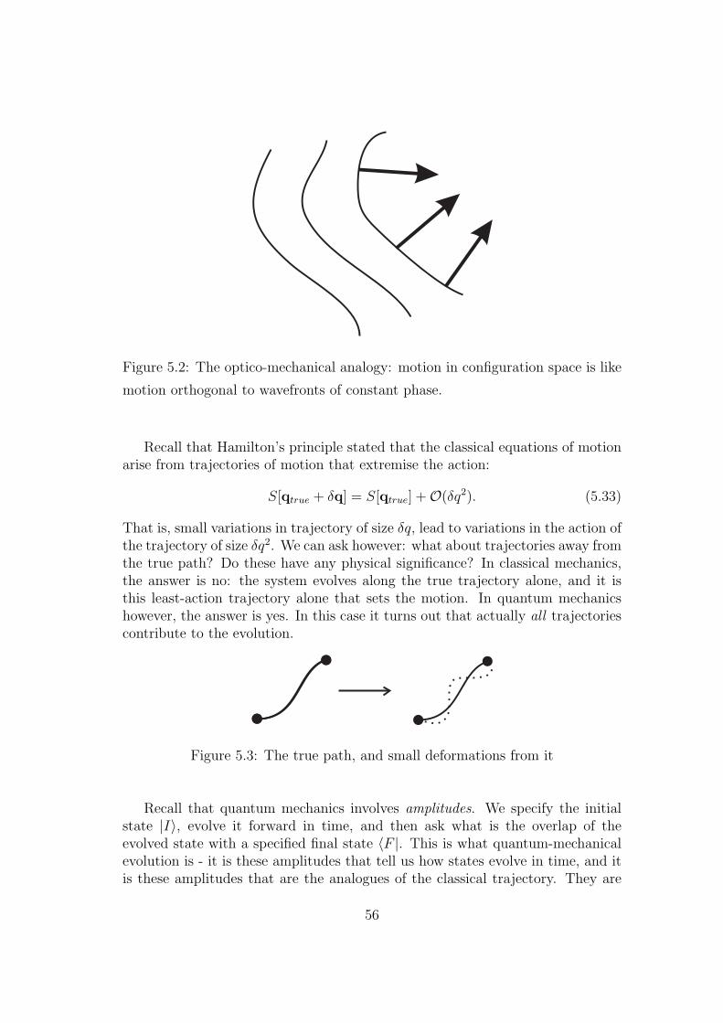
Figure 5.2: The optico-mechanical analogy: motion in configuration space is like
motion orthogonal to wavefronts of constant phase.
Recall that Hamilton’s principle stated that the classical equations of motionarise from trajectories of motion that extremise the action:
S[qtrue + δq] = S[qtrue] +O(δq2). (5.33)
That is, small variations in trajectory of size δq, lead to variations in the action ofthe trajectory of size δq2. We can ask however: what about trajectories away fromthe true path? Do these have any physical significance? In classical mechanics,the answer is no: the system evolves along the true trajectory alone, and it isthis least-action trajectory alone that sets the motion. In quantum mechanicshowever, the answer is yes. In this case it turns out that actually all trajectoriescontribute to the evolution.
Figure 5.3: The true path, and small deformations from it
Recall that quantum mechanics involves amplitudes. We specify the initialstate |I⟩, evolve it forward in time, and then ask what is the overlap of theevolved state with a specified final state ⟨F |. This is what quantum-mechanicalevolution is - it is these amplitudes that tell us how states evolve in time, and itis these amplitudes that are the analogues of the classical trajectory. They are
56
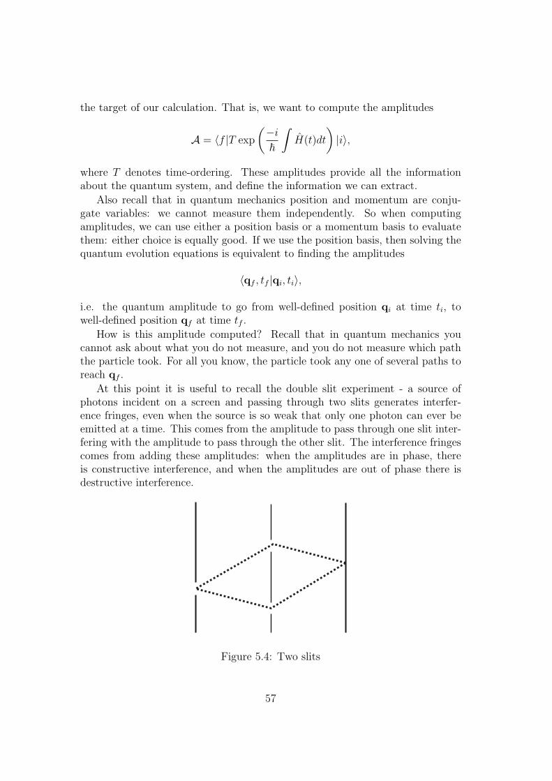
the target of our calculation. That is, we want to compute the amplitudes
A = ⟨f |T exp
(−i~
∫H(t)dt
)|i⟩,
where T denotes time-ordering. These amplitudes provide all the informationabout the quantum system, and define the information we can extract.
Also recall that in quantum mechanics position and momentum are conju-gate variables: we cannot measure them independently. So when computingamplitudes, we can use either a position basis or a momentum basis to evaluatethem: either choice is equally good. If we use the position basis, then solving thequantum evolution equations is equivalent to finding the amplitudes
⟨qf , tf |qi, ti⟩,
i.e. the quantum amplitude to go from well-defined position qi at time ti, towell-defined position qf at time tf .
How is this amplitude computed? Recall that in quantum mechanics youcannot ask about what you do not measure, and you do not measure which paththe particle took. For all you know, the particle took any one of several paths toreach qf .
At this point it is useful to recall the double slit experiment - a source ofphotons incident on a screen and passing through two slits generates interfer-ence fringes, even when the source is so weak that only one photon can ever beemitted at a time. This comes from the amplitude to pass through one slit inter-fering with the amplitude to pass through the other slit. The interference fringescomes from adding these amplitudes: when the amplitudes are in phase, thereis constructive interference, and when the amplitudes are out of phase there isdestructive interference.
Figure 5.4: Two slits
57
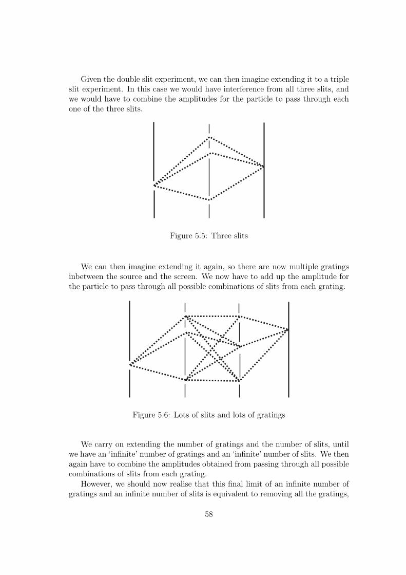
Given the double slit experiment, we can then imagine extending it to a tripleslit experiment. In this case we would have interference from all three slits, andwe would have to combine the amplitudes for the particle to pass through eachone of the three slits.
Figure 5.5: Three slits
We can then imagine extending it again, so there are now multiple gratingsinbetween the source and the screen. We now have to add up the amplitude forthe particle to pass through all possible combinations of slits from each grating.
Figure 5.6: Lots of slits and lots of gratings
We carry on extending the number of gratings and the number of slits, untilwe have an ‘infinite’ number of gratings and an ‘infinite’ number of slits. We thenagain have to combine the amplitudes obtained from passing through all possiblecombinations of slits from each grating.
However, we should now realise that this final limit of an infinite number ofgratings and an infinite number of slits is equivalent to removing all the gratings,
58

so that we now have photon propagation in free space, and summing over allpossible paths from initial position to final position.
Figure 5.7: An infinite number of slits and an infinite number of gratings
In this limit, the physics of the double slit experiment (different paths in-terfere) compel us to find the amplitude by summing over the amplitude of allpossible paths,
A =
∫D(paths) Amplitude(path). (5.34)
Feynman realised that the correct prescription here was that the amplitude for
any individual path q(t) is exp(
iS[q(t)]~
).
We can then obtain the quantum amplitude as
A = ⟨qf , tf |qi, ti⟩
=
∫Dq(t) exp
(iS[q(t)]
~
), (5.35)
where we have restricted to paths that start at qi and end at qf . We will statethat this works (a derivation is beyond the scope of this course), and that thisdoes indeed fully reproduce ‘conventional’ Hamiltonian quantum mechanics in itsentirety. In fact, for many advanced applications such as quantum field theory theFeynman path integral above is far more useful than the Hamiltonian approach.
The Feynman path integral requires that we sum over all possible paths frominitial to final state, weighting each path by exp
(iS~
). The biggest subtlety in
this tends to be the measure factor: when we say summing overall paths, whatdoes the measure factors
Dq(t)
actually mean? How do we actually compute with this? What does it mean tosum over an infinite number of possible paths? Although this is a bit confusing atfirst, this issue can be understood, eventually making the Feynman path integralone of the most powerful tools in theoretical physics.
59
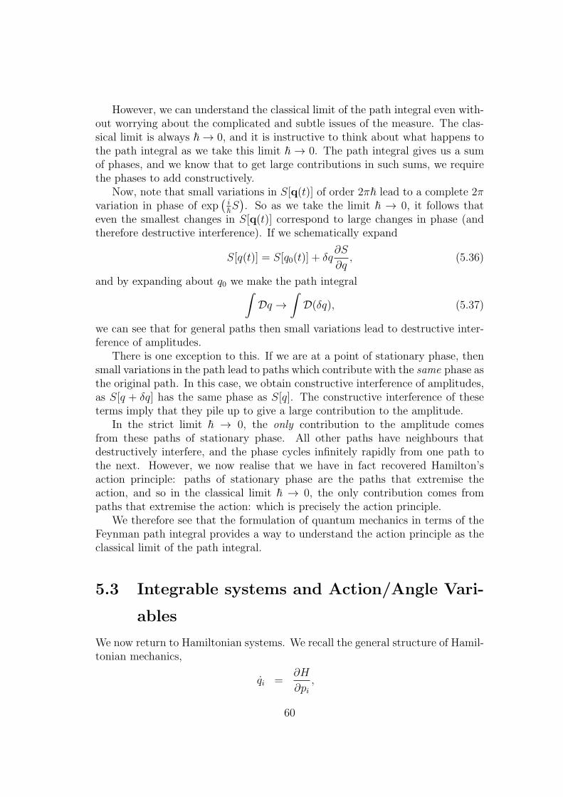
However, we can understand the classical limit of the path integral even with-out worrying about the complicated and subtle issues of the measure. The clas-sical limit is always ~ → 0, and it is instructive to think about what happens tothe path integral as we take this limit ~ → 0. The path integral gives us a sumof phases, and we know that to get large contributions in such sums, we requirethe phases to add constructively.
Now, note that small variations in S[q(t)] of order 2π~ lead to a complete 2πvariation in phase of exp
(i~S). So as we take the limit ~ → 0, it follows that
even the smallest changes in S[q(t)] correspond to large changes in phase (andtherefore destructive interference). If we schematically expand
S[q(t)] = S[q0(t)] + δq∂S
∂q, (5.36)
and by expanding about q0 we make the path integral∫Dq →
∫D(δq), (5.37)
we can see that for general paths then small variations lead to destructive inter-ference of amplitudes.
There is one exception to this. If we are at a point of stationary phase, thensmall variations in the path lead to paths which contribute with the same phase asthe original path. In this case, we obtain constructive interference of amplitudes,as S[q + δq] has the same phase as S[q]. The constructive interference of theseterms imply that they pile up to give a large contribution to the amplitude.
In the strict limit ~ → 0, the only contribution to the amplitude comesfrom these paths of stationary phase. All other paths have neighbours thatdestructively interfere, and the phase cycles infinitely rapidly from one path tothe next. However, we now realise that we have in fact recovered Hamilton’saction principle: paths of stationary phase are the paths that extremise theaction, and so in the classical limit ~ → 0, the only contribution comes frompaths that extremise the action: which is precisely the action principle.
We therefore see that the formulation of quantum mechanics in terms of theFeynman path integral provides a way to understand the action principle as theclassical limit of the path integral.
5.3 Integrable systems and Action/Angle Vari-
ables
We now return to Hamiltonian systems. We recall the general structure of Hamil-tonian mechanics,
qi =∂H
∂pi,
60
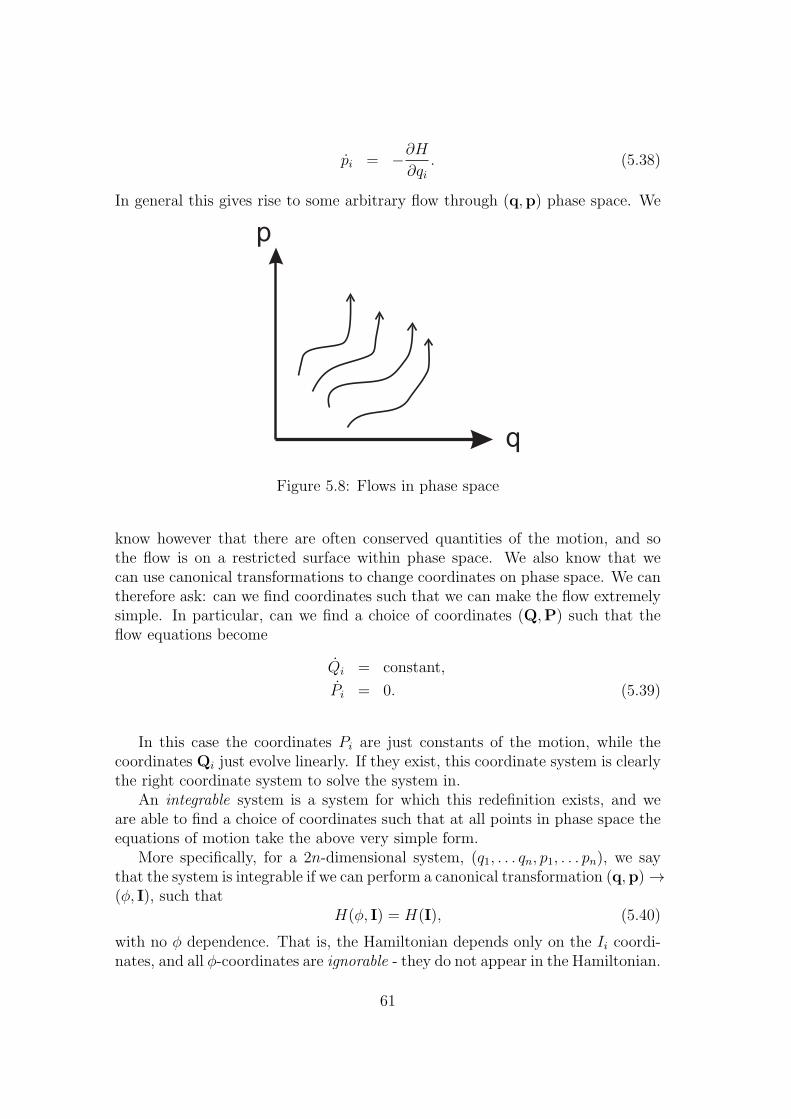
pi = −∂H∂qi
. (5.38)
In general this gives rise to some arbitrary flow through (q,p) phase space. We
p
q
Figure 5.8: Flows in phase space
know however that there are often conserved quantities of the motion, and sothe flow is on a restricted surface within phase space. We also know that wecan use canonical transformations to change coordinates on phase space. We cantherefore ask: can we find coordinates such that we can make the flow extremelysimple. In particular, can we find a choice of coordinates (Q,P) such that theflow equations become
Qi = constant,
Pi = 0. (5.39)
In this case the coordinates Pi are just constants of the motion, while thecoordinates Qi just evolve linearly. If they exist, this coordinate system is clearlythe right coordinate system to solve the system in.
An integrable system is a system for which this redefinition exists, and weare able to find a choice of coordinates such that at all points in phase space theequations of motion take the above very simple form.
More specifically, for a 2n-dimensional system, (q1, . . . qn, p1, . . . pn), we saythat the system is integrable if we can perform a canonical transformation (q,p) →(ϕ, I), such that
H(ϕ, I) = H(I), (5.40)
with no ϕ dependence. That is, the Hamiltonian depends only on the Ii coordi-nates, and all ϕ-coordinates are ignorable - they do not appear in the Hamiltonian.
61

Q
P
Figure 5.9: What we would like the flow in phase space to look like
In this case we call the ϕ coordinates angle variables and the I coordinatesaction variables. When can we do this? We state the following theorem dueto Liouville (we do not call this Liouville’s theorem to avoid confusion with theprevious Liouville’s theorem on conservation of volume in phase space).
Suppose we have a Hamiltonian system with n constants of motion Ii, i =1, . . . , n, such that their Poisson brackets all mutually vanish:
[Ii, Ij] = 0.
Then the system is integrable and a set of action/angle variables exist.The proof of this is beyond the scope of the course. It can be found for
example in the book by Arnold.If we can succeed in finding action/angle variables, then the evolution equa-
tions are
ϕi =∂H
∂Ii= ωi, (5.41)
Ii = −∂H∂ϕi
= 0. (5.42)
and so we have
ϕi = ωit+ Ai, (5.43)
Ii = Bi, (5.44)
where ωi, Ai and Bi are constants.For bound systems with a finite range (generally due to energy conservation),
the ϕi are periodic with a conventional range of 2π (this explains the origin ofthe name ‘angle’ variable).
62

I
Figure 5.10: The global transformation to action/angle variables
Note that integrability, or the existence of action/angle variables, is a globalproperty of the system. Locally we can always do a transformation of variablesto make the system look integrable. The difficulty is in extending this localtransformation to a global transformation. Roughly, you can always straightenout a set of flow lines locally - the problem is always to extend this to do thisglobally.
Figure 5.11: The local transformation to action/angle variables: always possible!
You might want to think here about similarities to the problem of combing all the hair on a surface flat.
You can do this on a cylinder, but not on a sphere. Locally of course the two surfaces are the same - the
difference is global. In a similar way integrability is a global property of a system, not a local one.
We now focus on 1-dimensional systems with a time-independent Hamiltonian.In this case H is a conserved quantity, and so by the above theorem action/anglevariables always exist. How do we find them?
q
p
Figure 5.12: A general potential giving rise to periodic motion
Suppose we have periodic motion in a general potential. What are the ac-tion/angle variables? We know that I, as a conserved quantity, must be somefunction of energy, I = I(H).
63

We will state the correct answer, and then show why it is correct.
I =1
2π
∮p dq, ϕ =
∂
∂I
∫ q
0
p dq. (5.45)
That is, I(E) is the phase space area enclosed by an orbit of energy E. To verifythat this is the correct expression for I, we want to show that ∂H
∂I= ω, where ω
is the frequency of the orbit.To prove this, we note that for a classical mechanical system
p =√2m√E − V (q), (5.46)
and as we also have p = mq, we can write
dt =
√m
2
dq√E − V (q)
. (5.47)
If we integrate over one period of the motion, we have
2π
ω= T =
√m
2
∮dq√
E − V (q)
=
∮ √2m
(d
dE
√E − V (q)
)dq
=d
dE
∮ √2m
∫ √E − V (q) dq
=d
dE
∮p dq
= 2πdI
dE. (5.48)
We therefore have ω = dEdI, as required for action/angle variables.
Let us illustrate the calculation of action/angle variables by calculating ac-tion/angle variables for the 1-dimensional simple harmonic oscillator. The orbitsof the harmonic oscillator are well known: they correspond to ellipses in phase
space, with a maximal range of q of√
2Ek
and a maximal range for p of√2mE.
We first want to determine the action variable. This is given by the areaenclosed under this ellipse, and so
2πI = π
√2E
k
√2mE = 2πE
√m
k, (5.49)
which we can write as
I =E
ω0
. (5.50)
64

q
p
2mE
2E
k
Figure 5.13: Orbits for the simple harmonic oscillator
To determine ϕ, we have
ϕ =∂
∂I
∫ q
0
p dq =∂
∂I
∫ q
0
√2mω0I − kmq2 dq
= mω0
∫ q
0
dq√2mω0I − kmq2
= arcsin
(q
√mω0
2I
). (5.51)
This angle variable ϕ then evolves as
ϕ = ω0t+ β, (5.52)
as an angle variable should.
65


![Classical Mechanics - people.phys.ethz.chdelducav/cmscript.pdf · References [1]LandauandLifshitz,Mechanics,CourseofTheoreticalPhysicsVol.1., PergamonPress [2]Classical Mechanics,](https://img.dokumen.tips/doc/110x75/5e1e9832bac1ea74484e9601/classical-mechanics-delducavcmscriptpdf-references-1landauandlifshitzmechanicscourseoftheoreticalphysicsvol1.jpg)


![[Kibble] - Classical Mechanics](https://img.dokumen.tips/doc/110x75/552056344a79596f718b4715/kibble-classical-mechanics.jpg)