Class 28 Get Ready….. Height and Weight Is CM or Inches the better predictor of KG? – Whichever has the lower standard error Will also have a variety

Class 28

Get Ready….

Height and Weight• Is CM or Inches the better predictor of KG?

– Whichever has the lower standard error• Will also have a variety of better stats

– NOT whichever has the bigger coefficient• A multiple regression lets you test

– H0: all b’s = 0 (nothing in the model matters)– H0: b1=0 given all the other b’s

• When using both CM and INCHES– We reject H0 b1=b2=0– We fail to reject H0 b1=0 given b2– We fail to reject H0 b2=0 given b1

• You need either CM or INCHES but not both– Because they are highly correlated

• Regressions ALWAYS go thru the sample averages

Things I expect you will know

• How to interpret a regression using p-1 dummy variables– The p possible forecasts will equal the sample average Y

for each of the p groups– The intercept is the average of the left-out group– The coefficients are differences in group averages.– The p-value/significance F will match that from ANOVA

single factor


• How to interpret a residual (error)– It is Y - – It is the distance each Y is from the line.– Positive means above the line.– They measure the difference between actual Y

and expected Y (based on the X’s)– The most over-weight girl (for her height) is the

girl with the largest positive residual.• Check the box to get residuals.

• How to interpret a coefficient in a multiple regression.– It measures the change in expected Y for a unit change

in that X keeping all other Xs constant.• If I keep miles and stops constant and change from williams

to spencer, expect 0.97 hours less.• If I change from Williams to Spencer, expect 0.33 hours more.

– It is the easy way to answer some questions.• If the previous rating goes from 17.5 to 20, how will the

expected ratings change? (by 0.18571 per point)


• How to use a regression model to calculate a point forecast.– Plug and chug.

• I use SUMPRODUCT• You must know what Xs to plug in.• It is a package deal….you must know and plug in ALL

the Xs.


• How to use a regression model to calculate a probability.– The question gives you the Y.– You Plug and chug to get the .– You calculate t = (Y - )/ standard error– Use t.dist.rt( t , dof)

• Dof is n – total number of regression terms.

– Requires the FOUR assumptions.


• If the coefficient of X1 changes when X2 is included in the model…..– You know X1 and X2 are correlated.– You can use the two regression results to tell whether

X1 and X2 are positively or negatively correlated.• Ds was positively correlated with Miles• Fact was negatively correlated with Stars• Nobel was positively correlated with Yanks• Speed was positively correlated with Dcorporate• Exam 1 was negatively correlated with Exam 2.


UNDERSTANDING

CoefficientRegression Table

Constant 13.24615

Fact 1.40107


Constant 12.568Fact 1.799Stars 1.259

Oh…Fact Movies had fewer Stars!


Constant 13.24615

Fact 1.40107




Secret Formula

�̂�=�̂�−𝑏1

𝑏2

Regress Y on X1

Regress Y on X1 and X2


Regress X2 on X1

Secret Formula


Constant 13.24615

Fact 1.40107



�̂�=1.40 −1.80

1.26

Regress Y on X1



�̂�=− 0.32Regress X2 on

X1

UNDDERSTANDING


Constant 13.24615

Fact 1.40107




UNDERSTANDING


Constant 13.24615

Fact 1.40107



Fact Movies averaged 0.32 fewer Stars!

Secret Formula

• Scatter-plot the cloud• It is up to YOU to interpret the results.• Don’t assume X causes Y

– Y might be causing X– Both might be caused by Z

• Don’t assume better fitting lines are better at forecasting– They usually are not…..too good a fit means too

complicated a model…..means poorer performance.

Regression is the line through a cloud of points

Class 28 AssignmentVariable School

Graduation Rate

% of Classes Under 20

Student/Faculty Ratio

Alumni Giving Rate

Description The name of theUniversity

Percentage of enrollees who graduate

Percentage of Classes offered with <= 20 students.

Number of students enrolled divided by total number of faculty

Percentage of living alumni who gave to the University in 2000

Mean 83.042 55.729 11.542 29.271Median 83.5 59.5 10.5 29Mode 92 65 13 13Standard Deviation

8.607 13.194 4.851 13.441

Skewness -0.282 -0.501 0.582 0.370Minimum 66 29 3 7Maximum 97 77 23 67Count 48 48 48 48

1. Test the hypothesis that graduation rate and alumni giving rate are (linearly) independent. We expect universities with higher graduation

rates to have higher mean giving rates. [15 points]

• Regress Giving Rate on Grad Rate• Check if coeff is positive• Divide reported p-value (found in two places)

by 2.• Reject if less than 0.05.

CoefficientsStandard

Error t Stat P-value

Intercept -68.76 12.58 -5.46 1.82E-06

Graduation Rate 1.18 0.15 7.83 5.24E-10

2. If the graduation rate of school A is 5 percentage points higher than that of school B, how much higher do we expect school A’s giving rate to be? [10 points]

• Using the above regression (graduation rate is all we know), the expected giving rate will be 1.18*5 = 5.9 percentage points higher for school A.

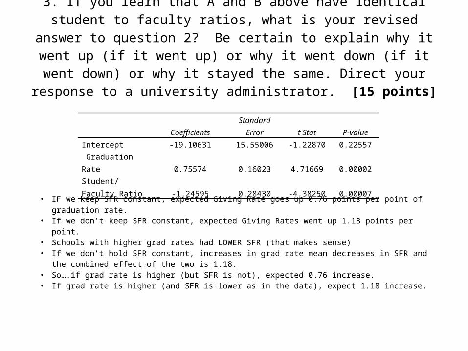
3. If you learn that A and B above have identical student to faculty ratios, what is your revised answer to question 2? Be certain to explain why it went up (if it went up) or why it went down (if it went down) or why it stayed the

same. Direct your response to a university administrator. [15 points]

Coefficients Standard Error t Stat P-valueIntercept -19.10631 15.55006 -1.22870 0.22557 Graduation Rate 0.75574 0.16023 4.71669 0.00002Student/Faculty Ratio -1.24595 0.28430 -4.38250 0.00007

• IF we keep SFR constant, expected Giving Rate goes up 0.76 points per point of graduation rate.

• If we don’t keep SFR constant, expected Giving Rates went up 1.18 points per point.

• Schools with higher grad rates had LOWER SFR (that makes sense)• If we don’t hold SFR constant, increases in grad rate mean decreases in SFR

and the combined effect of the two is 1.18.• So….if grad rate is higher (but SFR is not), expected 0.76 increase.• If grad rate is higher (and SFR is lower as in the data), expect 1.18 increase.

4. Provide a point forecast of alumni giving rate for a university with graduation rate of 80, 65 percent of its classes with 20 or fewer students, and a student/faculty ratio of 20. [25 points]

• The best model includes Grad Rate and SFR (% classes <20 not needed)

Coefficients Standard Error t Stat P-valueIntercept -20.7201 17.5214 -1.1826 0.2433 Graduation Rate 0.7482 0.1660 4.5082 0.0000% of Classes Under 20 0.0290 0.1393 0.2084 0.8358Student/Faculty Ratio -1.1920 0.3867 -3.0823 0.0035

CoefficientsIntercept -19.10631 Graduation Rate 0.75574Student/Faculty Ratio -1.24595 Intercept 1 Graduation Rate 80Student/Faculty Ratio 20POINT FORECAST 16.43

Don’t Use this variable.

Use this model.

Plug and Chug.

5. Of the 48 universities in the data set, which one has the most surprisingly low alumni giving rate? [10 points]

• The university with the most negative residual.

• Use the best model, ask for residuals, find the minimum.

• MICHIGAN!

6. Bo notices that some of the 48 have “university” in their names, some have “college” and the rest have “institute”. Bo wonders whether these names are predictive of student/faculty ratio?

(Formulate and test a relevant hypothesis.) [25 points]

• Three groups (p=3)• ANOVA or Regression of SFR on 2

dummies.

SUMMARY OUTPUT

ANOVA

df SS MS FSignificance

FRegression 2 103.7348 51.8674 2.3290 0.1090Residual 45 1002.1818 22.2707Total 47 1105.9167

Coefficients Standard Error t Stat P-valueIntercept 11.8636 0.7114 16.6754 0.0000Dcollege -0.3636 3.4120 -0.1066 0.9156Dinstitute -7.3636 3.4120 -2.1582 0.0363

Get Ready…..

• More practice problems (answers) on website.

• I’ll host Sunday night Office Hours.• I am available Monday and Tuesday until

2pm.– Email [email protected]– Check the website to see where I am…you

are welcome to join us.

mailto:[email protected]

Documents

Class 28 Get Ready….. Height and Weight Is CM or Inches the better predictor of KG? – Whichever has the lower standard error Will also have a variety