CIVIL ENGINEERING STUDIES

UILU-ENG-88-2006

CIVIL ENGINEERING STUDIES STRUCTURAL RESEARCH SERIES NO. 542

ISSN: 0069-4274

NUMERICAL EVALUATION OF DOMAIN AND CONTOUR INTEGRALS FOR NONLINEAR FRACTU E MECHANICS:

FORMULATION AND IMPLE ENTATION ASPECTS

By ROBERT H. DODDS, JR .

. and .. . PEDRO M. VARGAS

A Report on a Research Project Sponsored by the DAVID TAYLOR RESEARCH CENTER METALS AND WELDING DIVISION

ANNAPOLIS, MARYLAND

DEPARTMENT OF CIVIL ENGINEERING UNIVERSITY OF ILLINOIS AT .

. URBANA-CHAMPAIGN ,.; .. URBANA, ILLINOIS AUG.UST 1988

50212-101 REPORT DOCUMENTATION /.1 .. ./;,REPORT NO. .

PAGE UILU-ENG-88-2006 3. Recipient's ACCHlion No.

4. Title and Subtitle Numerical Evaluation of Domain and Cont·our Integrals for

5. Repo"rt Date

August 1988 Nonlinear Fracture Mechanics: Formulation and Implementation Aspect

~--~-------------------.. ------------------ .. --------------~----------- t----------------------~ 7. Author{s)

R. H. Dodds, Jr. and P. M. Vargas 9. Performing Organization Name and Address

University of Illinois at Urbana-Champaign Department of Civil Engineering 205 N. Mathews Avenue Urbana, Illinois 61801

12. Sponsoring Organization Name lind Address

David Taylor Research Center Annapolis, MD 21402

15. Supplementary Notes

8. Performing Organization Rept. No.

SRS 542 10. Project/Task/Work Unit No.

11. Contract(C) or Grant(G) No.

(C)

CG)

13. Type of Report & Period Covered

~--------------------------~

1------------------------------------_. ------_. . .. -----.----.-----.-..... - .. . - ._" ----._.--------------1 ·16. Abstract (Limit: 200 words)

The crack tip flux integral, denoted J, for local translations (Mode I) of a planar, curved crack front has potential application as a characterizing parameter in three-dimensional, nonlinear fracture mechanics. The integral, defined over a vanishingly small contour in a normal plane to the crack front, provides the pointwise value of the mechanical energy release rate. Arbitrary loading and material behavior are accommodated in the limit of a vanishing contour shrunk onto the crack front. Numerical evaluation of the integral in the context of finite element analysis necessarily leads to the development of computational procedures for non-vanishing, finite-sized contours. Such developments have proceeded along two lines with the corresponding introduction of "Domain Integral" (integrals over element volumes) and "Contour Integra1 1l (line integrals and area integrals) methods. Each approach leads to identical numerical values; selection of a procedure thus becomes a matter of convenience in element meshing and problem specification. This report describes the theoretical basis of each computational procedure, associated numerical algorithms, and details of the implementation in the general purpose analysis system POLO-FINITE. Example problems addressing 2-D and 3-D cracked structures for linear and nonlinear response under thermomechanical loading are presented to illustrate the general applicability of the procedures.

~-------------------------------------------------------------------------------------------------~ 17. Document Analysis a. Descriptors

Inelastic Fracture, Finite Elements, J-Integrals, Crack-Tip Fields, Numerical Techniques, Computer Software.

b. Identifiers/Open·Ended Terms

c. COSATI Field/Group

18. Availability Statement

Release Unlimited

(See ANSI-Z39.18)

19. Security Class (This Report)

UNCLASSIFIED 21. No. of Pages

50 r--------------------------~-------------------

20. Security Class (This Page)

UNCLASSIFIED See Instructions on Reverse

22. Price

OPTIONAL FORM 272 (4-77) (Formerly NTIS-35) Department of Commerce

NUME ICAl EVALUATION OF DOMAIN AND CONTOUR INTEGRALS FOR NONLINEAR FRACTURE MECHANICS:

FORMULATION AND IMPLEMENTATION ASPECTS

By

Robert H. Dodds, Jr.

and

Pedro M. Vargas

A Report on a Research Project Sponsored by the

DA VID TAYLOR RESEARCH CENTER

Annapolis, Maryland

University of Illinois Urbana, Illinois

August 1988

ABSTRACT

The crack tip flux integral, denoted J, for local translations (Mode 1) of a planar, curved crack front has potential application as a characterizing parameter in threedimensional, nonlinear fracture mechanics. The integral, defined over a vanishingly small contour in a normal plane to the crack front, provides the pointwise value of the mechanical energy release rate. Arbitrary loading and material behavior are accommodated in the limit of a vanishing contour shrunk onto the crack front. Numerical evaluation of the integral in the context of finite element analysis necessarily leads to the development of computational procedures for non-vanishing, finite,-sized contours. Such developments have proceeded along two lines with the corresponding introduction of Domain Integrals (integrals over element volumes) and Contour Integrals (line integrals and area integrals) methods. Each approach leads to identical numerical values; selection of a procedure thus becomes a matter of convenience in element meshing and problem specification. This report describes the theoretical basis of each computational procedure, associated numerical algorithms, and details of the implementation in the general purpose analysis system POLO-FINITE. Example problems addressing 2-D and 3-D cracked structures for linear and nonlinear response under thermomechanical loading are presented to illustrate the general applicability of the procedures.

-ii-

ACKNOWLEDGMENTS

This work was supported by the David Taylor Research Center, Annapolis, Maryland, Metals and Welding Division, Fracture and Fatigue Branch (Code 2814), through the ONR-ASEE Summer Faculty Research program. Computational support was provided by the Department of Civil Engineering Apollo Network made possible, in part, by grants from Apollo Computers, Inc. Graphical modeling software, PATRAN, was provided by PDA Engineering, Inc. The contribution of these organizations in support of this research is gratefully acknowledged.

-iii-

TABLE OF CONTENTS

Section No. Page

1. Introduction . . . . . . . . . . . . . . . . . . . . . . . . . . . . . . . . . . . . . . . . . . . . . . . . . .. 1

2. Crack Tip and Domain Integrals ................................. 3

2.1 Domain Integral Formulation ........................... ' ..... 4

2.2 Contour Integral Formulation. . . . . . . . . . . . . . . . . . . . . . . . . . . . . . .. 6

3. Numerical Procedures ......................................... 10

3.1 Domain Integral Procedures ................................ 10

3.1.1 Definition of the q-Function ......................... 10

3.1.2 Volume Integrals .. ~ ................................ 10

3.1.3 Crack Face Traction Integral. . . . . . . . . . . . . . . . . . . . . . . .. 11

3.1.4 Coincident Crack Front Nodes ....................... 12

3.1.5 Computation of f . .................................. 13

3.1.6 2-D Specialization ................................. 13

3.1.7 Output from Computations .......................... 14

3.2 Contour Integral Procedures ................................ 14

3.2.1 Definition of the Contours and Areas ................. 14

3.2.2 Contour Integral Evaluation. . . . . . . . . . . . . . . . . . . . . . . . .. 15

3.2.3 Area Integral Evaluation ............................ 15

3.2.4 Output from Computations .......................... 15

4. Commands For J-integral Processing ............................ 17

4.1 Outline of Process ........................................ 17

4.2 Input Error Correction .................................... 18

4.3 Initiating a Domain or Path Definition ....................... 18

4.4 Domain Definition. . . . . . . . . . . . . . . . . . . . . . . . . . . . . . . . . . . . . . .. 19

4.4.1 Crack Front Nodes ................................. 19

- iv-

4.4.2 q-Function Nodal Values ............................ 20

4.4.3 Element List ...................................... 20

4.4.4 Example.......................................... 20

4.5 Path (Area) Definition .................................... 21

4.5.1 Examples ......................................... 21

4.6 Domain and Path Maintenance ............................. 22

4. 7 Computational Requests ..... . . . . . . . . . . . . . . . . . . . . . . . . . . . . .. 22

4.7.1 Examples ...................................... " .. 23

5. Example Problems ............................................ 24

5.1 Domain Integral Example. . . . . . . . . . . . . . . . . . . . . . . . . . . . . . . . .. 24

5.1.1 Definition of Domains .............................. 27

5.1.2 Remote Axial and Crack Face Loadings ............... 28

5.1.3 Thermal Loading .................................. 29

5.2 Contour Integral Example ................................. 37

6. References ................................................... 42

-v-

LIST OF TABLES

Table No. Page

1 Current Capabilities for J-Integral Computation in POLO-FINITE . . . . .. 17

2 Domain Integral Results for Remote Tensile Loading ................. 29

3 Domain Integral Results for Crack Face Loading .................... 30

4 Domain Integral Results for Thermal Loading . . . . . . . . . . . . . . . . . . . . . .. 30

5 Summary of Computed I-values for Center-Crack Panel Example ..... 41

-vi-

LIST OF FIGURES

Figure No. Page

1 Infinitesimal Tubular Shaped Surface and Contour Enclosing Portion of Crack Front . . . . . . . . . . . . . . . . . . . . . . . . . . . . . . . . . . . . . . . . . . . . . . . . . . . . .. 4

2 Finite Volume for Use in Domain Integral Formulation ................. 5

3 Variation of Weight Function q Over Volume at Crack Front . . . . . . . . . . .. 6

4 Subregion of Infinitesimal Thickness Enclosing the Crack Front . . . . . . . . .. 7

Sa Isoparametric Element Showing Valid Contour Segments and Gauss Point Surfaces . . . . . . . . . . . . . . . . . . . . . . . . . . . . . . . . . . . . . . . . . . . . . . . . . . .. 9

Sb View of Element Mesh Near a Surface Flaw Showing Gauss Plane Used for Contour and Area Integral Evaluation ........................ 9

6 Thick Wall Cylinder with Internal Circumferential Crack ............... 24

7 Finite Element Mesh for Thick-Wall Cylinder with Internal Crack ....... 25

8 Partial Listing of FINITE Input for Tube Crack Analysis . . . . . . . . . . . . . .. 26

9 q-Function Along Crack-Front for First 5 Domains ................... 27

10 q-Function for Domain RING_ 4 ................................... 28

. 11 FINITE Input to Define Domains for 3--D Analysis . . . . . . . . . . . . . . . . . . .. 31

12 FINITE Generated Output for Crack Face Loading . . . . . . . . . . . . . . . . . . .. 32

13 Center-Crack Panel Geometry and Finite Element Model .............. 38

14 Near-Tip Mesh Refinement and Contours for J Computation ........... 39

15 FINITE Input to Define Contours for Center-Crack Panel .............. 39

-vii-

NUMERICAL EVALUATION OF DOMAIN AND CONTOUR INTEGRALS FOR NONLINEAR FRACTURE MECHANICS:

FORMULATION AND IMPLEMENTATION ASPECTS

1. Introduction

Finite element methods are especially powerful for computing the displacement, strain, and stress fields near crack-like defects in 2-D and 3-D structural configurations under general loading and material behavior. While the material response remains linear at the crack tip, numerical values of the stress-intensity factor, KJ , are readily obtained from asymptotic displacement substitution techniques using the computed near-tip nodal displacements. Alternatively, various conservation (line) integrals [20,21,24]' which generalize to surface and volume integrals in 3-D, may be evaluated to obtain the potential energy release rate, often denoted G, from which the stress-intensity factor is directly computed from the relation KJ = jE . G/(l - v2

) .

In most practical applications, material near crack-like defects experiences nonlinear deformation sufficient to invalidate the use of linear elastic fracture mechanics. The intensity of deformation along the crack front in such cases is often characterized by a pointwise value of the J-integral, derived by generalizing the conservation line integral to admit inelastic material behavior [1,4,7]. However, the penalty of generalization is the theoretical requirement for vanishingly small contours (or enclosing tubular-shaped surfaces) at the crack front and the associated requirement for accurate resolution of field variables near the crack front. The resulting crack tip flux integral defines the release rate of mechanical energy for local translations (Mode I) of a planar, curved crack front. This J-integral has potential application as a characterizing parameter in three-dimensional, nonlinear fracture mechanics. In two-dimensional approximations where plane stress-plane strain conditions prevail, the J-integral directly controls the amplitude of the singular field near a sharp crack tip, as given by the HRR solutions [14,23], under certain limiting conditions involving material constitutive behavior and the extent of plastic deformation relative to the uncracked ligament size [1 7]. For large scale plasticity in two dimensions and for all situations in three-dimensions, there exists no direct theoretical connection between the value of the I-integral as defined above and the nature of the asymptotic near tip fields. Researchers are beginning to undertake computational studies, especially in 3-D, with the level of finite element mesh required to examine the nature of the crack tip fields and the relationship to J [3,5,10,11,12,16,22]. The increasing availability of supercomputers is making these studies possible.

Numerical evaluation of the I-integral in the context of finite element analysis necessarily leads to the development of computational procedures applicable for non-

1

vanishing, finite-sized contours. Such developments have proceeded along two lines with the corresponding introduction of Domain Integrals (integrals over element volumes) [10,11, 12,16] and Contour Integrals (line integrals and area integrals) [1,3,9,15] methods. Each approach -leads to identical numerical values; selection of a procedure thus becomes a matter of convenience in element meshing and problem specification.

This report describes the capabilities implemented in the POLO-FINITE structural mechanics system [23] for computation of I-integral values. Facilities are provided to compute J for Mode I conditions following a linear or nonlinear analysis for both 2-D and 3-D structural configurations. Two formulations and corresponding methods of numerical evaluation are provided: (1) Domain Integrals (D!) applicable in 2-D and 3-D; and (2) Contour Integral (CI) applicable in 2-D and 3-D. The Contour Integral method requires that the user specify a contour (integration path) enclosing the crack tip. For 3-D configurations, an integral defined over the planar area enclosed by the contour is required to maintain path independence unless contours are defined very near the crack tip. The Domain Integral method is a variant of the Virtual Crack Extension (VCE) technique [8,13]; it is more general and simpler for the analyst to specify. The analyst defines nodal values of a weight function which may be interpreted as the motion of material near the crack front due to a virtual crack extension. The numerical computations then involve the evaluation of an area integral in 2-D and a volume integral in 3-D. With the Domain Integral approach the analyst is relieved of the detailed specification of Gauss points and element orientations required with the Contour Integral method. For these reasons, the Domain Integral procedure i~ implemented for the niost general case and is the preferred method of I-integral evaluation.

The following section provides a more extensive discussion of Domain and Contour Integrals for 2-D and 3-D applications. The numerical procedures needed in the finite element evaluation of the integrals are developed in Section 3. Commands newly implemented in POLO-FINITE to support the computation of Domain and Contour Integrals are described in Section 4. Example problems addressing 2-D and 3-D cracked structures for linear and nonlinear response under thermomechanical loading are presented in Section 5 to illustrate the general applicability of the procedures.

2

2. Crack Tip and Domain Integrals

A local value of the mechanical energy release rate, denoted I (n), at each point 11 on a planar, stationary crack front under quasi-static loading is given by

lim ~ aUi 1(11) = [Wnl - G··-n·] dr '/ € ~ 0 f€ 1) aXl J

(2-1)

where W is the stress-work density, r is a vanishingly small contour which lies in the principal normal plane at 11, and n is the unit vector normal to r (see Fig. 1). All field quantities are expressed in the local orthogonal coordinate system, X1-X2-X3, at location 11 on the crack front.

This important result was first derived by Eshelby [7] and independently by Cherepanov [4], and later by others considering only mechanical energy balance for a local translation of the crack front in the X 1 direction (Mode 1). Any form of loading and arbitrary material behavior is permitted, provided that the limiting process is imposed on the contour r. Dynamic effects may be introduced by including the kinetic energy (1) with W in the first term of the integral. All proposed forms of path independent integrals (contour, area, volume) for application in fracture mechanics derive from Eq. (2-1) by specialization of the loading and material behavior.

Nakamura, et al. [19] have proven the local path independence of I on the actual shape of r in the limit as r --iIt 0+. To have both path independence and a non-vanishing, finite value (the integrability condition), the integrand of Eq. (2-1) must have order 1/rn, where n < 2. It is especially important to note that the quantity I defined by Eq. (2-1) has no direct relationship to the form of the near-tip strain-stress fields, except for very limited circumstances. For plane-stress and plane-strain conditions, with nonlinear elastic material response and small-scale yielding, I of Eq. (2-1) simplifies to the well-known I-integral due to Rice that controls the amplitude of the HRR singular fields and that exhibits global path independence. The role of I as a single parameter characterizing the near tip strain-stress fields for arbitrary loading (static, thermal, dynamic) in 2-D and 3-D configurations is the topic of much current research.

Limiting consideration to quasi-static loading in the context of infinitesimal strain theory (at least outside a finitely deformed process zone), the total strain, fij, is additively decomposed into elastic (e), inelastic (P), and thermal (t) components as

(2-2)

with the stress-work density defined as the stress work through the mechanical strains

(2-3)

3

Eqs. (2-1) to (2-3) form the basis of both the Domain and Contour Integral methods.

X2

Crack Front ~ ~

Fig. 1, Infinitesimal Tubular Shaped Surface and Contour Enclosing Portion of Crack Front

2.1 Domain Integral Fonnulation

The Domain Integral method is derived by considering a vanishingly small tube of length !:l. and radius E that encloses the crack front at point II (see Fig. 1). The contour r in Eq. (2-1) lies on the surface of the tube at point ll. Then, in the limiting case of vanishing il, Eq. (2-1) may be rewritten as

(2-4)

where the integration is now performed over the surface of the tube rather than along the contour. To obtain a volume integral over a finite domain, the vanishingly small tube is surrounded by a finite size, tubular shaped surface having enclosed ends (see Fig. 2).

Nikishkov and Atluri [11,12] suggested that an equivalent form of Eq. (2-4) may

be constructed as

J(1])/= f [Wnl-ai' aUi n,] q dA JA-AE J aXl J

(2-5)

where q = q(Xl' X2, X3) is an arbitrary but continuous function which is equal to zero on the enclosing tubular area, A, and is non-zero on Ae-; and f is the area under the q-function along the segment of the crack front, .L1 (see Fig. 3). The q-function is readily interpreted as the Virtual Crack Extension (VCE) although the formulation does not require such interpretation; the q-function is a mathematical device which allows the generation of an equivalent volume integral more naturally suited to finite-

4

Fig. 2, Finite Volume for Use in Domain Integral Formulation.

element computations. The divergence theorem is applied to recast Eq. (2-5) as a volume integral which yields (including applied crack face tractions),

J(t]) f= - f [W~i - ajj~~ ~i] dV JV-VfaXl aXl aXj

(2.,..6a)

- f [~~ -~-(aij~~)] q dV Jv-v£ aXl aXj aXl

(2-6b)

- f ti~L!i q dA JA1+A2 aXl

(2-6c)

+ f [Wnl-aij~l!.!.nj] q dS Sl-S2 aXl

(2-6d)

where all quantities are expressed in· the local Cartesian system at point ". This finite domain integral expression yields a weighted average value for J along the crack front over which f is non-zero. A 1 and A2 are the loaded portions of the crack faces on each side of the crack plane (X1-X3). S1 and S2 denote the end surfaces of the volume~ V, and may be taken to lie in the X1-X2 plane for convenience. Since this formulation is derived from purely mechanical energy balance, the effects of inelastic strains (thermal, creep, non-proportional plasticity) may be introduced through VI. In most instances, the volume Vf coincides with the crack front and is zero; thus the volume V

5

includes the crack tip elements (several cases in 2-D and 3-D exist for which integration over the crack tip elements can be avoided).

The last integral in Eq. (2-6) is omitted in this implementation without loss of generality by requiring that q vanish over the end areas 81 and 82 when they correspond to internal surfaces. On symmetry planes and traction free (external) surfaces, the integrand of Eq. (2-6d) vanishes independently of q. The integrand of Eq. (2-6c) vanishes if the crack faces are not loaded or if q = 0 on the loaded portions of the crack faces. Similarly, the integrand of Eq. (2-6b) vanishes for q = 0 or if the material is elastic and thermal loading in V is absent. By assuming the existence of an elastic potential function, W, such that the stresses are defined by Oij = a W / aEij , Eq. (2-6b) simplifies to

i aw a aUi i awP aEf/ [---(oij-)] q dV= [--Oij-] q dV v-v£ aXl aXj aXl v-v£ aXl aXl

(2-7)

where the equilibrium equations in the absence of body forces have been employed. For a nonlinear elastic material the terms wP and f!ij vanish.

q(Xl, XZ,X3) is most often de-fined to vary line- q ('I]) arly in the X1-X2 plane as shown

f = r q(TJ) dTJ See notes about q on S1 and 81

Fig. 3, Variation of Weight Function q Over Volume at Crack Front

2.2 Contour Integral Formulation

Extension of Eq. (2-1) to allow a finite, rather than vanishingly small, contour in the X1-X2 plane is accomplished by considering the fundamental definition of the conservation integral [24,26]

6

j = ( [Wnl - Ti aUj] d'L J~ aX1

(2-8)

where ~ denotes the complete surface enclosing a portion of the crack front of differentiallength d1J as illustrated in Fig. 4. Assuming that the crack faces r+, r are free of applied tractions, the above integral may be written as a contour integral over r (multiplied by d1J) and surface integrals over the planar areas denoted A+, A-. Noting that the outward normals to these two surfaces are parallel and in opposite directions, the sum of the two area integrals is given by the X3 derivative of integrand multiplied by d1J. Division of both sides of Eq. (2-8) by d1J yields the pointwise value for the integral as

Fig. 4, Subregion of Infinitesimal Thickness Enclosing the Crack Front

~ . aUj i aUj J = [Wnl - Tj- ] dr + a[Wnl - Ti-)]/aX3 dA

r aXl A aXl (2-9)

Re-writing the above expression as a separate contour and area integral yields

(2-10)

where Jc is a line integral evaluated over a remote contour and JA is an area integral evaluated over the planar surface enclosed by the contour. Substituting for the traction vector with the stress components, the final form of the contour integral is given by

( au-Jc = Jr [Wnl - aij ni ax~] dr (2-11)

The area integral is given by

7

f aw adt/ a aUi IA=- [--aij-+-(ai3-)] dA

A aXl aXl aX3 aXl (2-11)

where W has been separated into an elastic and inelastic component. The existence of an elastic potential from which total stresses are derived from the elastic· component of total strain is also assumed in reaching the above result. Equilibrium equations in the absence of crack face loadings and body forces are also employed. This form, proposed by Carpenter, et al. [3], includes the various special cases obtained in earlier 3-D contour formulations which imposed restrictions on material behavior. The first two terms of the area integral arise from the explicit partial derivative of the work density and should be retained for path-dependent (incremental) plasticity. The third term of the area integral vanishes as the contour shrinks to the crack tip as the integrand is nonsingular. If the material is homogeneous and nonlinear elastic, then aW/aXl = Gij(a€ij/axl)and the first and second terms of Eq. (2-11) vanish. Rice's 2-D,

path-independent I is easily recovered from Eqs. (2-9) by requiring a nonlinear elastic material and either plane-stress or plane-strain conditions.

The Contour Integral formulation implemented in POLO-FINITE is based on Eqs. (2-10) and (2-11) without the thermal loading capability. In the 2-D specialization only the contour integral is currently implemented. For 3-D evaluations, the near tip element mesh must be constructed such that element faces are normal to the generally curved crack front as illustrated in Fig. 5b. Contours and corresponding areas for integration are prescribed to lie in planes of Gauss points which are then normal or nearly normal to the crack front. Integration over Gauss point planes allows the most accurate values to be used in the computations. However, there is a mismatch between contours and the corresponding enclosed area since the area integration is performed over a complete Gauss plane within an element. The errors in this approximation are considered to be small especially when meshes are constructed with semi-circular shaped rings of elements enclosing the crack front. In such cases, the contour and area integrals may be individually generated and plotted as functions of radial distance from

.the crack tip, then summed to provide the total I-value at each radial distance (such computations provide confirming evidence of the path-independence of the computed I-values).

8

Valid Contour Segment

III Gauss Point

• Element Node

Gauss Point Plane

Fig. Sa, Isoparametric Element Showing Valid Contour Segments and Gauss Point Planes

Crack Front

-------. Gauss Plane Normal to Crack Front Thru Element Centers

Fig. 5b, View of Element Mesh Near a Surface Flaw Showing Gauss Plane Used for Contour and Area Integral Evaluation

9

3. Numerical Procedures

This section describes the numerical procedures developed to evaluate the Domain and Contour Integrals described previously. An understanding of these procedures is necessary for the correct use of the commands described in following sections.

3.1 Domain Integral Prncedures

3.1.1 Definition of the q-Function

Consistent with the isoparametric formulation, the q-function within an element is assumed to have the form

(3-1) i = }

where Qi are the specified values of the q-function at the element nodes. The user specifies: (1) nodes along the crack front included in the computations needed to evaluate f, (2) elements over which integrations are to be performed, (3) Qi at nodes over the volume, V, and (4) orientation of the crack front coordinate axes at the point T)

under consideration. To considerably simplify this process, linear interpolation of the q-function between values defined at the element corner nodes is available. Also, when collapsed elements are defined along the crack front with multiple coincident nodes, only one of the coincident nodes at each location needs to be specified; the computational routines locate the remaining coincident nodes and assign them the same value of q. Several options to provide the orientation of the crack front axes are available.

3.1.2 Volume Integrals

Noting that the integrand in Eq. (2-6d) always vanishes under the restriction on the q-function for areas S1 and S2, the remaining two volume integrals are numerically evaluated using the same Gaussian quadrature procedures adopted for element stiffness generation. The integral in Eq. (2-6a) presents no difficulties as both Wand the stresses are available at the Gauss point locations and the q-function derivative is readily computed from specified nodal values and Eq. (3-1). Gauss quadrature applied to Eq. (2-6a), denoted DM1, yields the expression for numerical computations as

~ aq aUi aq aXm DM} = - L [W--oij--]p det [-]p wp

p ax} ax} aXj arJm (3-2)

where the summation extends over all Gauss quadrature points (P) and wp denotes the

Gauss weight values. Cartesian derivatives of q and the displacements are obtained in the usual manner using the chain rule

(3-3)

10

and,

au; = ± ± aNI arJm Uil

aXl I m ar;m aXl (3-4)

where N is the number of element nodes.

The integrand in Eq. (2-6b) contains derivatives of quantities for which numerical values of the quantities themselves are known at the Gauss point locations. The quadrature requires that the derivatives of these quantities also be available at the integration points. To obtain the needed derivatives, the inelastic component of W, W, and the inelastic and thermal components of the total strain, Ett , are extrapolated to the element nodes using Lagrangian polynomials of the order corresponding to the numerical quadrature order. In 3-D, for example, the bi-linear Lagrangian polynomials are used for an integration order of 2x2x2 (this corresponds to the well-known Barlow extrapolation procedure [25]). Given nodal values of the functions, derivatives at the integration points are obtained using expressions similar to those of Eqs .. (3-3,4). The volume integral is then numerically evaluated using an expression of the form given in Eq. (3-2). Numerical tests have demonstrated that the procedure works very well for thermal strains which are non-singular at the crack tip and generally vary smoothly over the near-tip region. Insufficient tests have been conducted to verify the adequacy of the procedure for inelastic components of the work density and strain ..

For wedge elements, the total strains and work density are evaluated at the integration points and directly at the element nodes by the element strain-stress routines. The extrapolation procedure described above is unnecessary for these elements.

3.1.3 Crack Face Traction Integral

The crack face traction integral, Eq. (2-6c), may be evaluated directly using standard element face integration procedures if the components of the applied tractions are available at the element nodes. However, this data is not readily accessible during post-processing, especially for nonlinear analyses. Rather the equivalent nodal loads corresponding to the applied crack face tractions are available during post-processing for both linear and nonlinear analyses. The crack face integral is thus evaluated numerically using the expression

i ti aUi q dA =- .I I qz {auJ aXl}! {PilI Al+AZ aXl k z

(3-5)

where k is taken over elements with non-zero crack face tractions; I is taken over all element nodes on the loaded face; {P} is the vector of equivalent nodal loads at element node I due to the surface traction. Displacement derivatives at the element nodes needed in Eq. (3-5) are obtained by extrapolating derivatives computed at Gauss point locations. Lagrangian polynomials are again adopted for the extrapolation. Not only is

11

this technique more accurate than directly evaluating derivatives at the element nodes, the difficulty in computing derivatives at nodes on the crack front due to the singularity is avoided (extrapolated derivatives are not singular). Numerical tests demonstrate that the approximate expression given in Eq. (3-5) works very well.

For wedge elements the extrapolation procedure is not utilized since displacement derivatives are computed directly at the element nodes by the strain-stress routines. However,' if quarter-point wedge elel?1ents are defined along the crack front, derivatives for the crack front nodes cannot be computed due to the vanishing determinant of the coordinate Jacobian. This case is detected by the element routines and a zero value for the derivative is computed. Contributions to the crack face integral by nodes along the crack front are thus not included in the summation of Eq. (3-5). The error should be negligible.

The computational routines determine which element faces are loaded by examining the equivalent nodal load vectors for the complete element. If an element vector indicates that more than one face is loaded, the lowest numbered element face is processed and a warning message is issued to the user. Because this procedure was adopted (thereby eliminating the need to respecify crack face loads during J computation) , crack face loads and thermal loads should not be specified in the same loading condition -- the computational routines will mistake the equivalent nodal loads due to the thermal loading for crack face loading.

Users must include in the list of elements to process, all elements with crack face loading if any node on the face has a non-zero q value.

3.1.4 Coincident Crack Front Nodes

The use of degenerated brick-type elements along the crack front leads to multiple, coincident nodes. To simplify specification of the q-function over the domain volume, the q-value for only one of the coincident nodes at such crack front positions is required. The remaining coincident nodes at corresponding crack front positions are located and assigned the same value for q. The procedure followed to. locate coincident nodes is outlined below.

For each user specified node along the crack front, the numerical procedure constructs coordinates for a rectangular prism centered at the node, then locates all other nodes of the model that lie within the prism. Such nodes are treated as coincident with the specified node and assigned the same q-value. Dimensions for the rectangular prism are defined as follows:

a. if only one node on the crack front is specified by the user (a 2-D model), the box sides extend ± R x tol where R is the distance from the coordinate system origin to the specified node. If the specified node is at the origin (R = 0), the box extends ± 10-~

12

b. for 2 or more nodes specified along the crack front (3-D models), the prism extends ± R x tal about the node, where R is the distance between the first two listed nodes on the crack front.

In both cases, the value 0.001 is currently specified for tal.

3.1 .5 Computation of f

The area under the q-function along the crack front, denoted J, is required to normalize J for arbitrary magnitudes of the specified q-function in Eq. (2-5), see also Fig.3. Thus, f may be interpreted as area of crack extension represented by a virtual crack extension q. The value of f is defined by

(3-6)

which is numerically evaluated using Gauss quadrature as

f = I I N/(1]p) q/ [jdxi + dx~ ]p Wp (3-7) p /

where the functional form of q over the segment of crack front under consideration, a :::; 1] :::; c, is specified by the user to vary in a piecewise linear, parabolic or cubic manner. Lagrangian interpolating functions, N/(1]) , are used to construct the piecewise functions for q along the crack front. The length of crack front over a :::; 1] ~ c is computed with the expression

L = L [jdxi + dx~ ]p wp (3-8) p

and is displayed for checking purposes.

3.1.6 2-D Specialization

For plane-stress and plane-strain models, the volume integrals simplify to area integrals and the area integral for the face traction integral simplifies to a line integral. The g-function needs to be specified at only one crack tip node; the same value will be assigned automatically to the other coincident nodes at the tip. The area under the q-funct~on along the crack front, J, is replaced by the specified q-value at the crack tip node.

Integration over crack tip elements can be avoided if there are no inelastic strains and no crack face loading. Nodes on crack tip elements (and surrounding elements if desired) are specified to have a constant q-value with q diminishing to zero at some remote ring of nodes enclosing the tip. The crack tip elements make no contribution to the integrals since the q-derivative vanishes. The element list can thus omit them. A similar procedure may be followed to obtain a thickness average J for through cracks

13

modeled in 3-D, i.e., where the local crack front axes have identical or very nearly identical orientation along the front.

3.1.7 Output from Computations

The printed output displayed during Domain Integral computations is organized in a hierarchial manner by loading condition (load step in a nonlinear analysis), then by each user specified domain. For each domain, the integral values are displayed for each element of the domain. The values printed for each element in a domain are labeled DM1 through DM5 and correspond to the terms in Eqs. (2-6) as follows

(3-9)

(3-10)

(3-11)

(3-12)

DMs = - I I qz {aUi/aX l}T {Pi}z (3-13) " z

The sum of these integrals over all elements of the domain is displayed followed by f, the area under the q-function along the crack front. The I-integral value is printed as the sum of the integrals divided by f The units of I are F - L/L2.

For 2-D specializations, the element thicknesses are not included in the integrals of Eqs. (3-9 to 3-13). The value of f is thus the specified value of q at the crack tip. The thickness effect cancels in the printed value of the total integrals divided by f and the units of J remain F - L/ L 2 •

For each loading condition, the average, maximum, and minimum I values are summarized in tabular form.

3.2 Contour Integral Procedures

3.2.1 Definition of the Contours and Areas

Numerical evaluation for the contour integral is performed in a piecewise fashion over the portion of the total path within each element. To enable the use of Gauss integration, paths are restricted to follow lines of constant ~,1] or ~ within each element ( ~,1] for 2-D elements). The Gauss points are numbered sequentially in ~ ~ 1] ~ ~ . The ordering of Gauss points on the path defines the positive direction of the contour. The positive contour direction should be specified counterclockwise about

14

the local X3 axis on the crack front (otherwise J will have a negative value). For 2-D, the integration orders of 2x2 and 3x3 are supported; for 3-D the uniform integration orders of 2x2x2 and 3x3x3 are supported.

For 3-D, the area enclosed by the contour must also be defined. This is accomplished by specifying Gauss point surfaces (planes) over which one of the three isoparametric coordinates ~,1] or ~ remains constant. This is illustrated in Fig. Sa. Thus, for the 2x2x2 integration order, there are six (6) surfaces of Gauss points. The surfaces 1 and 2 correspond to ~ = 0.577, - 0.577, respectively. Gauss surfaces 3 and 4 correspond to 1] = 0.577, - 0.577, and Gauss surfaces 5 and 6 are defined by S = 0.577, -0.577. Similarly, for the 3x3x3 integration order, there are nine (9) sur-faces of Gauss points. Surfaces 1, 2, and 3 are defined by ~ = 0.778,0.0, - 0.778, respectively. Tl:J.e remaining six surfaces are numbered according to this pattern.

Note that contour and area integration schemes are not available for wedge elements in 3-D.

3.2.2 Contour Integral Evaluation

Each term of the integrand in Eq. (2-11) is directly available at the Gauss points on the contour segment within an element. The quadrature scheme thus adopted is a 2 or 3 point Gauss rule for the path segment in an element.

3.2.3 Area Integral Evaluation

The area integral in Eq. (2-12) vanishes for the 2-D capabilities currently implemented. In 3-D, each term of the integrand involves derivatives of functions for which the values of the functions themselves are known at the Gauss quadrature points. This area integral is thus analogous to the second volume integral in the Domain Integral formulation, see Eq. (2-6b). The procedure of extrapolating the integrand to the element nodes using Lagrangian polynomials is also used for generation of the area integrand. Once nodal values of the integrand are known, the required derivatives at the Gauss points are obtain using standard isoparametric techniques.

The third term of the area integral in Eq. (2-12) is non-singular at the crack tip and vanishes for contours defined very near the crack tip, i.e., just outside the singularity elements. The first two terms of the integrand are identical to those of the second volume integral in the Domain Integral formulation and are unbounded at the crack tip. As for the Domain Integral, the numerical procedures for these two terms must be considered suspect until further evaluations of the performance can be conducted.

3.2.4 Output from Computations

The printed output displayed during Contour Integral computations is organized in a hierarchial manner by loading condition (load step in a nonlinear analysis), then by

15

each user specified contour (area). For each contour (area), the integral values are displayed for each element. The values printed for each element are labeled IC1, IC2, IA1, IA2, fA3 and correspond to the terms in Eqs. (2-11 and 2-12) as follows

~ au·

fC2 == - a .. n·-' df r IJ I a

e Xl

IAl == - f awP dA JAe aXl

L ad:·t

IA2 == aij_I_J dA Ae aXl

IA3 = - f ~ (ai3 aUi) dA

JAe aX3 ax!

(3-14)

(3-15)

(3-16)

(3-17)

(3-18)

In addition, the length of the contour segment or Gauss plane area is provided for each element as well as total lengths or areas.

Totals of the contour and area integrals are provided for each path. Similarly, average values, minimums, and maximums are provided for each loading condition.

16

4. Commands For J-Integral Processing

4.1 Outline of Process

The computational procedures described in the previous section may be invoked following a linear or nonlinear analysis of a structure modeled with isoparametric elements. Data describing the contours or weight functions for domain integrals are provided by the analyst and computations requested. This process may occur immediately following the analysis in the same program execution or through any number of restarts. For linear analysis, the structure containing elements and nodes that define the crack may appear at any level in a structural hierarchy; for nonlinear analysis all nonlinear elements must appear in the highest level structure as usual. Table 1 summarizes the currently implemented capabilities of the Domain Integral and Contour Integral methods.

Capability Domain Integral Contour Integral

2-D 3-D 2-D 3-D

Nonlinear Elastic Deformation Yes Yes Yes Yes

Inelastic Deformation Yes Yes No Yes

Thermal Loading Yes Yes Yes No

Crack Face Loading Yes Yes No No

Body Forces No No No No

Thermo-Plastic Deformation No No No No

Brick Elements Yes Yes Yes Yes

Wedge Elements N.A. Yes N.A. No

Table 1, Current Capabilities for I-Integral Computation in POLO-FINITE

The I-integral computation subsystem is entered via the sequence of two FINITE commands

POST( -PROCESS)

I( -INTEGRAL)

The POST-PROCESS command requests that FINITE initiate post-processing activities; the J-INTEGRAL command indicates which type of secondary analysis results are to be computed. To exit the post-processing system, enter the command

EXIT

which returns control of execution to 'the usual FINITE processors. Commands to request output, displacement/strain/stress· computation, to define/modify structures, etc.

17

may then be given. A STOP command may also be entered in the post-processing subsystem to terminate execution without a prior EXIT command.

At the completion of a linear analysis or a nonlinear analysis (for at least one load step), the sequence of actions listed below is usually followed to define the additional data for I-integral computations and to request results.

1. During the same execution as the analysis or during a restart execution, enter the postprocessing J-integral subsystem using the two commands described above.

2. Define any number of domains for Domain Integral computations or paths for Contour Integral computations. The DEFINE DOMAIN and DEFINE PATH commands are used for this purpose. Domains and paths are not associated with the definition of a structure and as such may be referenced to compute J for any structure as appropriate.

3. Issue a COMPUTE J-INTEGRAL command to request the computation of J for any number of specified domains/path and loading conditions/steps for a structure. Tabular results are printed automatically to the current output device during the computations.

4. Define new domains/paths, delete existing domains/paths, display domain/path definitions, and repeat (3) as desired.

5. Terminate J-integral processing with the EXIT command and issue additional FINITE structural processing commands or STOP.

4.2 Input Error Correction

When an invalid I-integral command is entered during execution, an internal error flag is set by the command interpreters. Numerical computations will not be attempted if an uncanceled error flag exists when the COMPUTE J -INTEGRAL command is encountered. Users executing FINITE interactively may cancel the error flag with a RESET command prior to issuing a COMPUTE command (which implies that the incorrect data has been re-entered correctly).

4.3 Initiating a Domain or Path Definition

New domains and paths may be defined at any point during I-integral processing. The command to initiate the definition is

{DOMAIN}

DEFINE <id> PATH

( <orientation> )

where <id> is either a <label> or a <string>. The <orientation> option is defined by

ROTATE [{~} <angle in degrees:numr> ]

(USE) POINTS ORIGIN <point> X <point> Y <point>

where <point> is a structure node or coordinate point number.

18

Each domain/path defined must have a unique identifier. Identifiers may not exceed 16 characters in length. A domain and a path with identical names are not permitted.

By default, the structure X-Y-Z coordinate axes are assumed to coincide with the local crack-tip axes, X1-X2-X3. In such cases the <orientation> part of the command may be omitted. In other cases, the <orientation> option specifies the relationship between the structure and crack-tip axes. The orientation may be specified in one of two ways. First, the ROTATE option· defines a Y-Z-X sequence of rotations about the structure axes necessary to align them with the local crack-tip axes corresponding to some location on the crack front. The second option uses the three-point method with three nodes (or a combination of nodes and coordinate points) to orient the crack-tip axes. The directionfrom the ORIGIN point to the X point defines the local crack-tip X1 axis. Similarly, the direction from the ORIGIN point to the Y point defines the local crack-tip X2 axis. The X3 axis is then computed from the vector cross product to form a right handed orthogonal system.

Several examples of the DEFINE command are

DEFINE DOMAIN PHEE_90 ROTATE Y 86.23

DEFINE PATH LOCAL_ONE ORIGIN 123 X 43 Y 98

4.4 Domain Definition

The domain definition consists of: (1) nodes on the portion of the crack front under consideration and the order of q-function interpolation along the front, (2) the list of structure nodes with non-zero q-function values and an optional flag requesting linear interpolation of q within each element from corner node values, and (3) the list of elements to be included in the computations. The commands to specify this information may be given in any convenient order following the DEFINE DOMAIN command. The domain definition terminates with the END OF DOMAIN command.

4.4.1 Crack Front Nodes

The command to define structure nodes on the crack front for the domain has the form

( LINEAR } FRONT (NODES) <node list:integerlist> ~ QUADRATIC (VERIFY)

\ CUBIC

where the ordering of nodes must follow increasing X3. The specified interpolation order defines the variation of q and the coordinates along the crack front for computation of the f term. The default order is LINEAR if a keyword is not specified. For the

19

QUADRATIC order, the number. of front nodes must follow the sequence 3, 5, 7, 9, etc.; for the CUBIC order the number of crack front nodes must follow the sequence 4, 7, 10, 13, etc. The interpolation order indicated with this command is not checked for compatibility with the interpolation order of the adjacent crack-tip elements. Only one (1) node number is required input for 2-D analyses and the keyword may be omitted.

When the crack is modeled with collapsed elements, there are multiple coincident nodes at locations along the front. Only one of the coincident nodes should be specified at such points in this command. The remaining coincident nodes are located automatically and included in subsequent processing. A list of the other nodes coincident with each front node specified in this command is printed if the keyword VERIFY appears as the last item of the command.

4.4.2 q-Function Nodal Values

Non-zero nodal values of q over the domain are defined with the command

Q( - V ALUES) [<nOde list:integerlist> <q :real> ] (LINEAR)

where the nodal q-values must be of class <real> to be distinguished from the list of node numbers. The LINEAR flag is passed to element computational routines to request linear interpolation of q-values from specified corner node values. Except for crack front nodes, mid-side nodes and mid-face nodes (Lagrangian elements) may thus be omitted from the above list. The LINEAR flag does not apply to nodes (and associated coincident nodes) appearing in the list of crack front nodes. The computational routines are informed of the nodes along the crack front such that LINEAR interpolation may be omitted as appropriate.

4.4.3 Element List

The list of all elements to be included in the computations is defined with the command

ELEMENTS <inte g er list>

Elements that should be included are: (1) those over which q is not constant, (2) those with loaded crack faces or thermal loading over which q is not zero everywhere.

4.4.4 Example

The following example illustrates the complete definition of a domain named A.

DEFINE DOMAIN A ROTATE Y -35.8 FRONT NODES 24 87 45 QUADRATIC VERIFY Q-VALUES 87 1.0 45 1.5 23 28 95 0.5 48 56 2.5,

120-140 BY 2 1.2 LINEAR ELEMENTS 1-30 BY 2

END OF DOMAIN

20

4.5 Path (Area) Deimition

The specification of paths (contours) and areas for integration are combined into one command of the form

ELE11ENTS <integerlist> {POINTS} <integerlist> FACE

«keyword:label or string»

Any number of ELEMENTS commands of this form may be used to complete the definition. The ordering of elements in each command is immaterial. The POINTS option implies the definition of a path segment through the list of elements; FACE implies a plane of Gauss points for area integration in the list of elements. The <integerlist> following POINTS or FACE defines the Gauss point numbers for a path segment or the single plane of Gauss points for an area integral.

The Gauss point list provided for a path segment is checked for consistency during computations by the element dependent routines. The implied order of integration indicated by the number of Gauss points listed in the path segment must agree with the integration order used in the element for the analysis (2x2, 3x3x3, etc.). Gauss points listed in the path segments must follow a counterclockwise pattern about the positive crack-tip X3 axis. The 2-D elements currently process only contour integrals and ignore the keyword.

For 3-D configurations, the contour integrals are specified in the same manner as for 2-D problems. The <keyword> is passed to the element dependent routines which examine it's content to determine the type of computation. The keyword to indicate the definition is a path segment for contour integration is CONTOUR. Similarly, the keyword to indicate the definition is an area segment for area integration is AREA. The keyword cannot be omitted for 3-D computations. The ordering of Gauss point planes is described earlier in section 3.2.

4.5.1 Examples

The following examples of complete path and area definitions illustrate the command syntax

DEFINE PATH RING_INSIDE ROTATE Z -90 ELEMENTS 1-15 BY 2 POINTS 1-3 ELEMENTS 26 28 33-40 POINTS 9 8 7

END OF PATH DEFINE PATH TWO ORIGIN 120 X 223 Y 300

ELEMENTS 2-30 BY 2 POINTS 7 8 9 ~CONTOUR~ END OF PATH DEFINE PATH AREA_ONE ROTATE Y 43 Z 120 X 54 _

ELEMENTS 1-36 BY 6 FACE 5 ~AREA~ ELEMENTS 50-80 BY 3 FACE 1 ~AREA~

END OF PATH

21

4.6 Domain and Path Maintenance

The current definition of domains and paths may be displayed with the command

{ DOMAIN} [{ <id:label or string>} ]

DISPLAY PATH ALL

Similarly, domains and paths may be deleted with the command

DELE1E {~:;:m} [Cd:1ab::r string> } ] Examples of these commands are

DISPLAY DOMAINS ONE TWO ABC DELETE PATHS ALL DELETE DOMAINS ONE , 123_ABC'

4~'7 Computational Requests

A C01\1PUTE command for i-integrals requests the system to perform the necessary computations and to output results in tabular form. For linear analysis, the command has the following form

COMPUTE I( -INTEGRAL) <domain/path list> «structure id>

«substructure list» ) «loading list»

where the <path/domain list> has the syntax listed below

The default options in this command are:

1. Omission of the <path/domain id list> implies ALL paths/domains currently defined.

2. Omission of the <structure id> implies the last structure mentioned in a COMPUTE, ACCESS, or STRUCTURE command.

3. Omission of the <loading list> implies all loadings that have results available for use.

The syntax of the <structure id>, the subordinate <substructure list>, and the <loading list> are as described in Chapter 2. The following restrictions also apply when the CO:MPU1E command is specified:

1. If individual domain/path names are specified, each one must be supplied as a class <string> data item to prevent ambiguities in the command syntax. For example, domains/ paths with the names 'ALL', 'STRUCTURE_DMA', etc. are thus valid.

22

2. A COMPUTE command which contains a <substructure list> implies that domain/path definitions refer to elements/nodes in the last structure appearing in the <substructure list>. Separate COMPUTE commands are required for each substructure - the J processing system does not automatically traverse the substructure hierarchy as does the OUTPUT command.

3. The COMPUTE J command does not automatically jorce the generation oj required analysis results as does the OUTPUT command. Users are responsible for insuring that displacements, strains, and stresses for those structures (and substructures) and loading conditions necessary for J evaluation have been computed. When needed but missing results are encountered, computations for the loading condition are omitted. This procedure is adopted to minimize computational effort for recovery of strains and stresses since only those elements directly involved in J computations must have strains and stresses available.

The J processing subsystem performs extensive diagnostics prior to and during computations. When missing data, invalld data, or inconsistencies are encountered, the order of processing is modified to allow continued execution. Error messages are issued to the user describing the problem and action taken. For example, an invalid domain having an element number out of range is simply deleted from the list of those processed.

For nonlinear analysis, the keyword NONLINEAR and a <step list> are required as shown below

CO:MPUTE NONLINEAR I( -INTEGRAL) <domain/path list>

«structure id> «substructure list» ) «loading id> ) «step list»

where <domain/path list> and <structure id> are the same as described above for linear analysis. Only one-loading name may be specified and it must have been declared as type NONLINEAR during the structural definition process. The <step list> follows the syntax described in Chapter 3 for CO:MPUTE and OUTPUT commands. The same restrictions and defaults listed above for linear analysis also apply for nonlinear analysis except that displacement, strain, and stress results for all elements are always available if the nonlinear analysis for the load step has been completed.

4.7.1 Examples

The following examples illustrate the various forms of the CO:MPUTE J-INTEGRAL command.

COMPUTE J-INTEGRAL FOR DOMAINS ALL STRUCTURE A/I, LOADINGS ABC D

COMPUTE J PATHS 'ONE' 'TWO'

COMPUTE NONLINEAR J FOR DOMAINS 'A' 'B', STRUCTURE X LOADING TENSION STEPS 3-6, 20-25

23

5. Example Problems

Two example problems are presented to demonstrate the I-integral capabilities including input commands and generated output. The first example illustrates the use of Domain Integral procedures for 3-D linear analysis including crack face and thermal loadings. The second example considers the nonlinear analysis of a tensile panel containing a center-crack modeled with 2-D plane strain conditions. The I-value is computed using the Contour Integration procedures. Details of the problem descriptions, FINI1E input data, and computed results are provided in the remainder of this section.

5.1 Domain Integral Example

The problem considered in this example is a thick wall cylinder containing a complete internal circumferential crack as shown in Fig. 6. The separately applied loads include a remote uniform tension, a uniform crack face traction (compression) equal in magnitude to the remote tensile loading, and a linear temperature gradient through the wall thickness. Although the structure and loadings are axisymmetric, a 3-D model is used for illustrative purposes.

Ro = 2.25 in._

Ri = 1.0 in.

Crack Length, a = 0.625in.

-..--

Modelled Segment

Fig. 6, Thick Wall Cylinder with Internal Circumferential Crack

The finite element mesh represents a 10 0 segment of the cylinder using one layer of 20-node isoparametric (Q3DISOP) elements. Details of the element mesh are given in Fig. 7. The crack front is enclosed by 6, 20-node elements each collapsed into a wedge .. Coincident nodes at the 00

, 50 and 10 0 positions along the crack front are free to displace in the crack plane (X-Z) , except for symmetry conditions on the 0 0 ,10 0

24

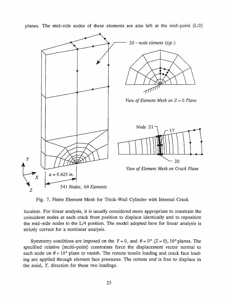
planes. The mid-side nodes of these elements are also left at the mid-point (L/2)

20 - node element (typ.)

View of Element Mesh on Z = 0 Plane

Y

View of Element Mesh on Crack Plane

2 541 Nodes, 64 Elements

Fig. 7, Finite Element Mesh for Thick-Wall Cylinder with Internal Crack

location. For linear analysis, it is usually considered more appropriate to constrain the coincident nodes at each crack front position to displace identically and to reposition the mid-side nodes to the L/4 position. The model adopted here for linear analysis is strictly correct for a nonlinear analysis.

Symmetry conditions are imposed on the Y = 0, and () = 0° (2 = 0), 10 0 planes. The specified relative (multi-point) constraints force the displacement vector normal to each node on () = 10 0 plane to vanish. The remote tensile loading and crack face loading are applied through element face pressures. The remote end is free to displace in the axial, Y, direction for these two loadings.

25

*RUN FINITE C

STRUCTURE TUBE NUMBER OF NODES 541 NUMBER OF ELEMENTS 64

COORDINATES X Y Z

1 1. 625000 0.000000 0.000000 2 1.618719 0.000000 0.000000

C INCIDENCES

1 11 56 51 6 12 57 52 7 9, 55 49 3 1 48 50 4 8 10,

5 2 64 525 529 538 524 527 530 539 526 523,

528 534 522 531 540 541 535 533 537, 536 532

C

ELEMENTS ALL TYPE GQ3DISOP NIX 2 NIY 2 NIZ 2 E 30000 NU 0.3 C

C

C

C

c

CONSTRAINTS

SYMMETRY CONDITIONS ON THETA = a FACE

1 W = 0.0 2 W = 0.0

538 W = 0.0 540 W = 0.0

C SYMMETRY CONSTRAINTS ON THETA = 10 DEGREES FACE (DISPLA. C NORMAL TO FACE MUST VANISH). C

4 0.1736482 U + 4 0.984808 W =0.0 541 0.1736482 U + 541 0.984808 W =0.0

C

LOADING REMOTE_TENSION '100 KSI REMOTE TENSION LOADING' ELEMENT LOADS FOR TYPE GQ3DISOP

58 63 UNIFORM GLOBAL FORCE Y P 100 FACE 3 C

C

LOADING CRACK_FACE '100 KSI COMPRESSION ON CRACK FACE' ELEMENT LOADS FOR TYPE GQ3DISOP

45 44 43 37 31 25 19 13 7 1 UNIFORM GLOBAL FORCE Y P 100 FACE 3

TRACE LINEAR DETAIL COMPUTE DISPLACEMENTS COMPUTE STRESSES STOP

Fig. 8, Partial Listing of F1NITE Input for Tube Crack Analysis

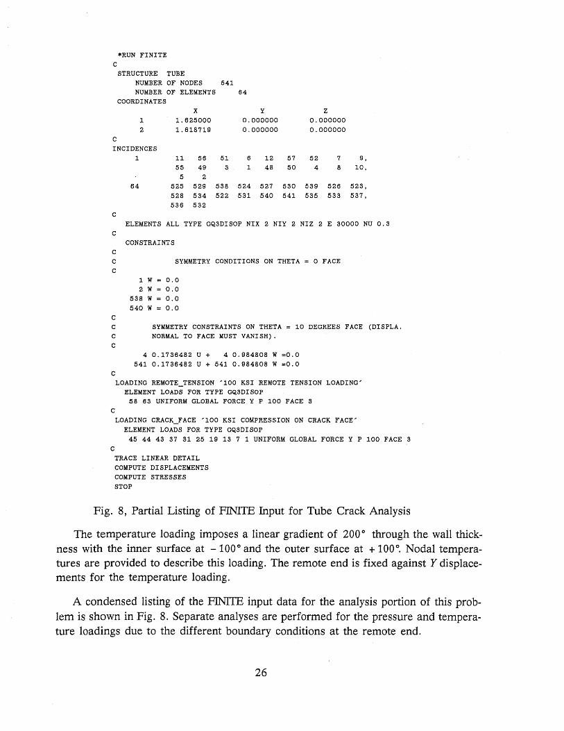
The temperature loading imposes a linear gradient of 200 ° through the wall thickness with the inner surface at -100° and the outer surface at + 100°. Nodal temperatures are provided to describe this loading. The remote end is fixed against Y displacements for the temperature loading.

A condensed listing of the F1NITE input data for the analysis portion of this problem is shown in Fig. 8. Separate analyses are performed for the pressure and temperature loadings due to the different boundary conditions at the remote end.

26

\

5.1.1 Definition of Domains

A total of 6 domains are defined to evaluate J for each loading condition. The variation of the weight function, q, along the crack front for the first 5 domains is illustrated in Fig. 9. These domains include only elements incident on the crack front and are typical of those employed to obtain pointwise J values along a generally curved crack front. For this axisymmetric problem, the exact J is constant along the crack front for each loading condition. Thus the sensitivity to the different q functions may be assessed. The three domains identified with the prefix SET_2 correspond directly to the usual nodal repositioning associated with traditional VeE procedures.

(21) (17) (20) (21) (17) (20) ........ 11--- Crack Front Nodes

SET 1 A SET 1 B

SET 2 A SET 2 B SET 2 C

Fig. 9, q-Function Along Crack-Front for First 5 Domains, Example 1

The last domain, denoted RING _ 4, typifies those used for J evaluation in throughcrack configurations (2-D and 3-D) to determine an average value over the complete crack front. In domain RING_ 4, all nodes associated with the inner most three rings of elements enclosing the crack front are specified to have identical q function values of 10. Nodes on the outer surface of the 4 th ring have q = 0, see Fig. 10. Thus, for the remote axial loading, the inner three rings of elements make zero contribution to J. For the crack face loading, elements of the inner three rings that lie on the crack face make non-zero contributions to the DM5 term while for the thermal loading all elements of the domain make non-zero contributions to the DM4 term.

For this element mesh, the global Yaxis of the structure corresponds to the local crack front X2 axis. Consequently, only rotations about the global Yaxis are required to align the structure and crack front axes.

27

Note: Only Corner Shown for Simplicity

q = 0 all nodes this ring & outer rings

q = 10 all nodes this ring & inner rings

Crack Front Nodes Are 21,17,20

Fig. 10, q-Function for Domain RING _ 4

5.1.2 Remote Axial and Crack Face Loadings

The Domain Integral results for J are employed to compute the corresponding stress-intensity factor using the plane strain conversion

K = /f!I-(2 x 1) I 1 2 -v (5-1)

where the finite element J value is multiplied by 2 to account for symmetry of the model about the crack plane. From superposition, both loadings cause identical near tip opening displacements and stress-intensity factors. The exact value (see Tada, et al. [18]) of the stress-intensity factor is

(5-2)

where the correction factor F has the value 1.089 for the alt of 0.5 in this problem. For both a remote tensile stress of 100 and a crack face loading in compression Qf 100, the exact stress-intensity factor is 152.6.

Results of the Domain Integral computations for the remote axial loading are summarized in Table 2. Table 3 summarizes results for the crack face loading. A listing of the input data to define the domains and to request computations is shown in Fig. 11. Sample output generated during the actual computations for the face loading is provided in Fig. 12 to illustrate the format of the results.

J ~e

J(fe Kexact Domain Id - I - I x 100%

2 Kjxact

SET 1 A 0.3361 149 -2.4 - -SET 1 B 0.3361 149 -2.4 - -SET 2 A 0.3375 149.2 -2.3 - -SET_2_B 0.3367 149.2 -2.3

SET 2 C 0.3375 149.2 -2.3 - -RING 4 0.3582 153.7 +0.7

Table 2, Domain Integral Results for Remote Tensile Loading (Kjxact = 152.6)

Table 2 shows that results for the remote loading are symmetric about (J = 50 and exhibit very small differences between domains. For the first 5 domains which involve only the crack tip elements, the results appear to be insensitive to the specified q-function variation along the crack front. The resulting stress-intensity factors for these 5 domains are consistently 2.4% below the exact value. For the last domain, RING_ 4, which avoids computations over elements at the crack tip, the J value is slightly larger and yields the exact stress-intensity factor. Results for crack tip domains 1-5 are lower than the exact value since the mid-side nodes of the crack tip elements are located at the mid-point (L/2) position, not the L/4 point position. Placement of the mid-side nodes at the 114 position introduces a more severe strain singularity in these elements and increases the stress-intensity factor.

Table 3 shows that results for the crack face loading are also symmetric about (J = 5 ~ The numerical values for 3 of the 5 domains agree exactly with results for the remote axial loading. The two domains which have negative values of the q-function (SET _2_ A and SET _2_ C) over a portion of the crack front yield considerably lower J

values. The last domain, RING_ 4, also predicts the exact J and stress-intensity factor for this loading. Additionally, numerical tests have shown that domain integral computations for crack face loadings exhibit larger errors when the quarter-point elements are employed.

5.1.3 Thermal Loading

Table 4 summarizes the results for the linear temperature gradient. The exact value of the stress-intensity factor is not known for this loading but a good estimate is available from the comp~ted displacements of nodes on the crack face singularity element. The stress-intensity factor from the displacements is given by

29

J ~e

Jte Kexact Domain Id - I - I x 100% 2 Kjxact

SET 1 A 0.3362 149 -2.4

SET 1 B 0.3362 149 -2.4 - -SET 2 A 0.2947 139.4 -7 - -SET 2 B 0.3588 153.8 0.8

SET 2 C 0.2936 139.4 -7 - -RING 4 0.3553 153.1 +Q.3

Table 3, Domain Integral Results for Crack Face Loading (Kjxact = 152.6)

J ~e

Kfe K!isPl Domain Id - x 100 I - I

2 KjiSPl x 100%

SET 1 A 0.6434 20.6 -3.3

SET 1 B 0.6434 20.6 -3.3 - -SET 2 A 0.6460 20.6 -3.3

SET 2 B 0.6445 20.6 -3.3

SET 2 C 0.6460 20.6 -3.3 - -RING 4 0.6857 21.3 0.0

Table 4, Domain Integral Results for Thermal Loading (Kjispl = 21.3)

K - E (ii 1 (y. - V ) I - 2(1 _ v2) V L fi _ 1 C B (5-3)

where Vc and VB are the opening mode displacements of the corner and mid-side nodes respectively (nodes 51 and 2 for example in this element mesh). This expression is obtained by substituting the known nodal displacements into the 2-D singular field (plane strain) and solving for the stress-intensity factor. Using the computed nodal displacements, the stress-intensity factor is found to be 21.3.

The Domain Int~gral results for the 5 domains involving only crack front elements predict identical values for the stress-intensity factor which are 3.3% less than the

30

*RUN FINITE FILE=20,,22 C

POST_PROCESS J-INTEGRAL

DEFINE DOMAIN SET_1_A ROTATE Y 10 FRONT NODES 21 17 20 QUADRATIC VERIFY Q-VALUES 21 10. 17 5.0 20 0.0 LINEAR

ELEMENTS 1-6 END

DEFINE DOMAIN SET_1_B ROTATE Y 5 FRONT NODES 21 17 20 QUADRATIC Q-VALUES 21 10.0 17 10. 20 10.0 LINEAR

ELEMENTS 1-6 END

DEFINE DOMAIN SET_1_C ROTATE Y 0 FRONT NODES 21 17 20 QUADRATIC Q-VALUES 21 0.0 17 5.0 20 10.0 LINEAR

ELEMENTS 1-6 END

DEFINE DOMAIN SET_2_A ROTATE Y 10 FRONT NODES 21 17 20 QUADRATIC VERIFY Q-VALUES 21 10. 17 0.0 20 0.0 LINEAR

ELEMENTS 1-6 END

DEFINE DOMAIN SET_2_B ROTATE Y 5 FRONT NODES 21 17 20 QUADRATIC Q-VALUES 21 0.0 17 10.0 20 0.0 LINEAR

ELEMENTS 1-6 END

DEFINE DOMAIN SET_2_C FRONT NODES 21 17 20 QUADRATIC Q-VALUES 21 0.0 17 0.0 20 10.0 LINEAR

ELEMENTS 1-6 END

DEFINE DOMAIN RING_4 ROTATE Y 5 FRONT NODES 21 17 20 QUADRATIC Q-VALUES 21 17 20 10.0,

145 146 150 151 164 165 179 181 180 182, 171 172 159 160, 98 103 117 132 133 124 112 51 56 70 85 86 99 104 118 134 135 125 113 52 57 71 87 88 66 10.0 LINEAR

ELEMENTS 1-24 END

77 65, 78,

COMPUTE J FOR DOMAINS ALL STRUCTURE TUBE LOADING FACE_PRESSURE

Fig. 11, FINITE Input to Define Domains for 3-D Analysis

nodal displacement value. The last domain, RING_ 4, predicts the same stress-intensity factor as the value derived from the nodal displacements at the crack tip.

31

J-INTEGRAL POST-PROCESSING

STRUCTURE: TUBE

LOADING: CRACK_FA TITLE: 100 KSI COMPRESSION ON CRACK FACE

CURRENT CPU TIME: 00:00:21.00

COINCIDENT NODES ON CRACK FRONT:

LISTED NODE

21 17 20

4

3

1

--- COINCIDENT NODES

7

9

6

12 23 11

14 30 13

18 38 15

26 39 25

28

27

33

32

DOMAIN INTEGRAL COMPONENTS

ELEMENT DM1 DM2 DM3 DM4

1 -0.5345E-02 0.1075E-Ol O.OOOOE+OO O.OOOOE+OO

2 -0.2183E-Ol 0.1187E+00 O.OOOOE+OO O.OOOOE+OO

3 0.2715E-Ol -0.1638E-Ol O.OOOOE+OO O.OOOOE+OO

4 -O.1340E-Ol 0.1631E+OO O.OOOOE+OO O.OOOOE+OO

5 O.2395E-Ol O.1524E-Ol O.OOOOE+OO O.OOOOE+OO

6 0.1190E-Ol O.8965E-Ol O.OOOOE+OO O.OOOOE+OO

TOTALS: O.2244E-Ol 0.3811E+00 O.OOOOE+OO O.OOOOE+OO

TOTAL OF DOMAIN INTEGRALS: 0.4767E+OO

AREA UNDER Q-FUNCTION ALONG CRACK FRONT: 0.1418E+Ol

LENGTH ALONG CRACK FRONT FOR THIS DOMAIN: O.2836E+OO

EDI / Q-FUNCTION AREA: 0.3362E+OO

35 44 45

34 42 43

DM5

0.73l6E-Ol

O.OOOOE+OO

O.OOOOE+OO

O.OOOOE+OO

O.OOOOE+OO

O.OOOOE+OO

0.73l6E-Ol

Fig. 12, FINITE Generated Output for the Crack Face Loading

32

47

46


STRUCTURE: TUBE




ELEMENT DM1 DM2 DM3 DM4 DM5 -------

1 -0.1067E-Ol 0.2153E-01 O.OOOOE+OO O.OOOOE+OO 0.1468E+00

2 -0.4350E-01 0.2377E+00 O.OOOOE+OO O.OOOOE+OO O.OOOOE+OO

3 0.5455E-Ol -0.3278E-Ol O.OOOOE+OO O.OOOOE+OO O.OOOOE+OO

4 -0. 2646E-Ol 0.3267E+00 O.OOOOE+OO O.OOOOE+OO O.OOOOE+OO

5 0.4820E-Ol O.S053E-Ol O.OOOOE+OO O.OOOOE+OO O.OOOOE+OO

6 0.2417E-Ol 0.l795E+00 O.OOOOE+OO O.OOOOE+OO O.OOOOE+OO

TOTALS: 0.4629E-Ol 0.7632E+00 O.OOOOE+OO O.OOOOE+OO 0.1468E+00

TOTAL OF DOMAIN INTEGRALS: 0.9563E+00

AREA UNDER Q-FUNCTION ALONG CRACK FRONT: O.2836E+Ol

LENGTH ALONG CRACK FRONT FOR THIS DOMAIN: 0.2836E+00

EDI / Q-FUNCTION AREA: 0.3372E+00


STRUCTURE: TUBE




ELEMENT DM1 DM2 DMS DM4 DM5

1 -0.5S45E-02 0.1076E-Ol O.OOOOE+OO O.OOOOE+OO 0.7368E-Ol

Fig. 12 cont'd, FINITE Generated Output for the Crack Face Loading

33

2 -0.2183E-01 0.1187E+00 O.OOOOE+OO O.OOOOE+OO O.OOOOE+OO

3 0.2715E-01 -0.1638E-01 O.OOOOE+OO O.OOOOE+OO O.OOOOE+OO

4 -0. 1340E-01 0.1631E+00 O.OOOOE+OO O.OOOOE+OO O.OOOOE+OO

5 0.2395E~01 0.1524E-Ol O.OOOOE+OO O.OOOOE+OO O.OOOOE+OO

6 0.1190E-01 0.8965E-01 O.OOOOE+OO O.OOOOE+OO O.OOOOE+OO

TOTALS: 0.2243E-01 0.3811E+OO O.OOOOE+OO O.OOOOE+OO 0.7368E-01


AREA UNDER Q-FUNCTION ALONG CRACK FRONT: 0.1418E+01

LENGTH ALONG CRACK FRONT FOR THIS DOMAIN: O.2836E+00



STRUCTURE: TUBE



COINCIDENT NODES ON CRACK FRONT:

LISTED NODE

ELEMENT

21 17 20

DM1

4 3

1

~-- COINCIDENT NODES

7 9

6

12 23 11

14 30 13

18 38 15

26 39 25


DM2 DM3

28 33 35

27 32 34

DM4

44 45

42 43

DM5

1 -0.1791E-02 0.3604E-02 O.OOOOE+OO O.OOOOE+OO O.4260E-02

2 -0. 7312E-02 0.3976E-01 O.OOOOE+OO O.OOOOE+OO O.OOOOE+OO


4 -0.4489E-02 0.5466E-01 O.OOOOE+OO O.OOOOE+OO O.OOOOE+OO

5 O.8026E-02 0.5106E-02 O.OOOOE+OO O.OOOOE+OO O.OOOOE+OO

6 O.3988E-02 O .. 3003E-01 O.OOOOE+OO O.OOOOE+OO O.OOOOE+OO

TOTALS: O.7519E-02 O.1277E+OO O.OOOOE+OO O.OOOOE+OO O.4260E-02


34

47

46




EDI I Q-FUNCTION AREA: 0.2947E+00


STRUCTURE: TUBE




ELEMENT DMl DM2 DM3 DM4 DM5 -------

1 -0.7136E-02 O.1436E-Ol O.OOOOE+OO O.OOOOE+OO 0.1394E+00

2 -0. 2914E-Ol 0.1585E+OO O.OOOOE+OO O.OOOOE+OO O.OOOOE+OO

3 0.3625E-Ol -0.2186E-01 O.OOOOE+OO O.OOOOE+OO O.OOOOE+OO

4 -0.178 9E-01 O.2178E+00 O.OOOOE+OO O.OOOOE+OO O.OOOOE+OO

5 0.3198E-Ol 0.2034E-01 O.OOOOE+OO O. OOOOE+OO, O.OOOOE+OO

6 O.1589E-Ol O.1197E+OO O.OOOOE+OO O.OOOOE+OO O.OOOOE+OO

TOTALS: 0.2995E-01 O.5088E+00 O.OOOOE+OO O.OOOOE+OO 0.1394E+00




EDI I Q-FUNCTION AREA: 0.3588E+00


STRUCTURE: TUBE




35

DOMAIN INTEGRAL COMPONENTS --------------------------

ELEMENT DM1 DM2 DM3 DM4 DM5 -------

1 -0.1791E-02 0.3605E-02 O.OOOOE+OO O.OOOOE+OO 0.3720E-02





6 0.3988E-02 0.3004E-Ol O.OOOOE+OO O.OOOOE+OO O.OOOOE+OO

TOTALS: 0.7515E-02 0.1277E+00 O.OOOOE+OO O.OOOOE+OO 0.3720E-02






STRUCTURE: TUBE




ELEMENT DMl DM2 DM3 DM4 DM5 -------

1 -0.7082E-18 -0.1014E-16 O.OOOOE+OO O.OOOOE+OO 0.2281E+00






7 0.1124E-18 0.8263E-17 O.OOOOE+OO O.OOOOE+OO 0.1335E+OO


36



10 -0.6646E-18 -0.1758E-16 O.OOOOE+OO O.OOOOE+OO O.OOOOE+OO

11 0.9713E-18 -0.S391E-17 O.OOOOE+OO O.OOOOE+OO O.OOOOE+OO

12 O.6308E-17 0.2573E-16 O.OOOOE+OO O.OOOOE+OO O.OOOOE+OO

13 0.2571E-17 -0.3095E-16 O.OOOOE+OO O.OOOOE+OO 0.1454E+00


15 0.1376E-16 -O.7613E-17 O.OOOOE+OO O.OOOOE+OO O.OOOOE+OO

16 -0.4425E-17 -0.5832E-17 O.OOOOE+OO O.OOOOE+OO O.OOOOE+OO



19 -0.1859E-Ol -0. 1470E-Ol O.OOOOE+OO O.OOOOE+OO 0.5586E-01

20 -0.2578E-Ol 0.5645E-Ol O.OOOOE+OO O.OOOOE+OO O.OOOOE+OO

21 O.4466E-01 -0.3096E-Ol O.OOOOE+OO O.OOOOE+OO O.OOOOE+OO

22 -0. 1500E-Ol 0.1620E+00 O.OOOOE+OO O.OOOOE+OO O.OOOOE+OO

23 0.4127E-Ol 0.6390E-01 O.OOOOE+OO O.OOOOE+OO O.OOOOE+OO

24 O.1714E-Ol 0.1643E+OO O.OOOOE+OO O.OOOOE+OO O.OOOOE+OO

----------- ----------- ----------- ----------- -----------TOTALS: 0.4370E-Ol 0.4010E+00 O.OOOOE+OO O.OOOOE+OO 0.5629E+OO



LENGTH ALONG CRACK FRONT FOR THIS DOMAIN: O.2836E+00


SUMMARY OF INTEGRATIONS FOR LOADING: CRACK_FA

AVERAGE OF DOMAIN INTEGRALS: 0.3303E+00

MINIMUM DOMAIN INTEGRAL: 0.2936E+OO

MAXIMUM DOMAIN INTEGRAL: 0.3588E+OO

»»> J-INTEGRAL COMPUTATIONS COMPLETED 00:00:36.00

STOP


5.2 Contour Integral Example.

The problem considered in this example is a flat panel containing a center throughcrack loaded by a remotely applied tensile stress. The geometry, loading, and finite

37

element mesh are shown in Fig. 13. Only one-quarter of· the panel is modeled due to the presence of two symmetry planes. Plane-strain response is prescribed for this 2-D

model. The material is characterized with an incremental plasticity model (J2 flow theory). The uniaxial stress-strain curve for the material has a yield point of 50 ksi and a Young's modulus of 30,000 ksi. A linear isotropic hardening model is employed with a tangent modulus following yield of 300 ksi.

A ~ A ~ A ~ ~ ~ A ~ ~

~ ofY

~ 8-node ele-\ ment (typ) H = 15.

~

o in.

'¥'" \ -

~

AI..

~ 1-./

~ \\ ... ~~ • 4 '-

a = 1.0 in.

W = 9.0 in.

79, 8-node elements, 282 nodes

Fig. 13, Center-Crack Panel Geometry and Finite Element Model, Example 2

38

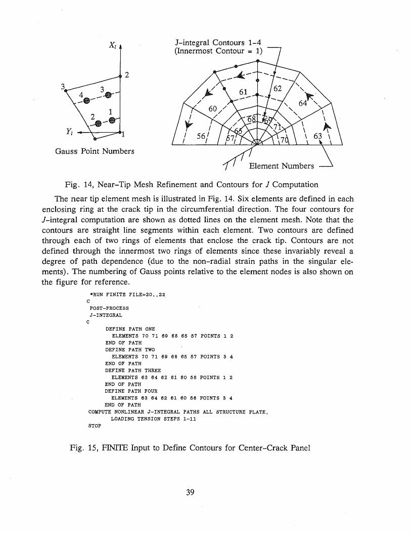
J-integral Contours 1-4 (Innermost Contour = 1)

2

Gauss Point Numbers

Element Numbers

Fig. 14, Near-Tip Mesh Refinement and Contours for J Computation

The near tip element mesh is illustrated in Fig. 14. Six elements are defined in each enclosing ring at the crack tip in the circumferential direction. The four contours for I-integral computation are shown as dotted lines on the element mesh. Note that the contours are straight line segments within each element; Two contours are defined through each of two rings of elements that enclose the crack tip. Contours are not defined through the innermost two rings of elements since these invariably reveal a degree of path dependence (due to the non-radial strain paths in the singular elements). The numbering of Gauss points relative to the element nodes is also shown on the figure for reference.

*RUN FINITE FILE=20, ,22 C

POST-PROCESS J-INTEGRAL

C

DEFINE PATH ONE ELEMENTS 70 71 69 68 65 57 POINTS 1 2

END OF PATH DEFINE PATH TWO

ELEMENTS 70 71 69 68 65 57 POINTS 3 4 END OF PATH DEFINE PATH THREE

ELEMENTS 63 64 62 61 60 56 POINTS 1 2 END OF PATH DEFINE PATH FOUR

ELEMENTS 63 64 62 61 60 56 POINTS 3 4 END OF PATH

COMPUTE NONLINEAR J-INTEGRAL PATHS ALL STRUCTURE PLATE, LOADING TENSION STEPS 1-11

STOP

Fig. 15, F1NITE Input to Define Contours for Center-Crack Panel

39

The remote stress is increased to 52.5 ksi in 10 steps of 5 ksi and a final step of 2.5 ksi. The solution does not converge at a remote stress of 55 ksi indicating that the plane-strain limit load lies between 52.5 and 55 ksi. Convergence in each load step is achieved within 2-3 iterations for the specified tolerance on the residual loads.

An input listing for definition of the contour integrals is shown in Fig. 15. The computed I values are summarized for each load step in Table 5. The results reveal very small variations between the four contours at each load step. To indicate the level of plastic deformation, the last column provides the average I-value at each load step scaled by the linear-elastic value of the energy release-rate, G = KJ(l - v2

) / E , at the same level of applied stress. The uniaxial yield stress of 50 ksi is adopted for scaling purposes. The results clearly show negligible variations of I among the four contours for the full range of loading. In the first load step, plastic deformation is confined to the crack tip elements and the computed I-value is only 1.4% larger than the linearelastic value derived from the stress intensity factor.

40

0 I p. - 11 12 13 14 lavg -

1 Oy G

1 0.10 0.002 0.002 0.002 0.002 0.002 1.014

2 0.20 0.010 0.010 0.010 0.010 0.010 1.016

3 0.30 0.022 0.022 0.022 0.022 0.022 1.022

4 0.40 0.039 0.039 0.039 0.039 0.039 1.033

5 0.50 0.062 0.063 0.062 0.063 0.063 1.051

6 0.60 0.092 0.093 0.093 0.093 0.093 1.082

7 0.70 0.129 0.132 0.131 0.132 0.131 1.121

8 0.80 0.177 0.181 0.180 0.182 0.180 1.179

9 0.90 0.245 0.250 0.250 0.253 0.249 1.292

10 1.00 0.381 0.384 0.381 0.385 0.383 1.607

11 1.05 1.406 1.402 1.391 1.391 1.398 4.848

Table 5, Summary of Contour J-Values for Center-Crack Panel

41

6. References

1. Amestoy, H.D., Bui" and Labbens, "On the definition of local path independent integrals in 3-D crack problems," Mechanics Research Communications, Vol. 8, (1981), 231-236.

2. Atluri, S.N. and Nakagaki, M., "Incremental path-independent integrals in inelastic and dynamic fracture mechanics," Engineering Fracture Mechanics, Vol. 20, (1984), 209-244.

3. Carpenter, w.e., Read, D.T., and Dodds, R.H., "Comparison of several path independent integrals including plasticity effects," International Journal of Fracture, Vol. 31, (1986), 303-323.

4. Cherepanov, G.P., "The propagation of cracks in a continuous medium," Journal of Applied Mathematics and Mechanics, Vol. 31, (1967) 503-512.

5. de Lorenzi, H.G., "On the energy release rate and the I-integral for 3-D," International Journal of Fracture, Vol. 19, (1982), 183-193.

6. Dodds, R.H., "Finite element evaluation of J parameters in 3-D," International Iournal of Fracture, Vol. 33, (1987), R7-R15.

7. Eshelby, J.D., "Energy relations and the energy momentum tensor in continuum mechanics," in Inelastic Behavior of Solids, M.F. Kanninen, et al. (eds), Mc GrawHill, NY, (1970).

Hellen, T.K., "On the method of virtual crack extension," International Iournal for Numerical Methods in Engineering, Vol. 9, (1975), 187-207.

9. Kishimoto, K., Aoki, S., and Sakata, M., "On the path independent j -integral," Engineering Fracture Mechanics, Vol. 13, (1980), 841-850.

10. Li, F.Z., Shih, C.F., and Needleman, A., "A comparison of methods for calculating energy release rates," Engineering Fracture Mechanics, Vol. 21, (1985), 405-421.

11. Nikishkov, G.P. and Atluri, S.N., "An equivalent domain integral method for computing crack-tip integral parameters in non-elastic, thermo-mechanical fracture," Engineering Fracture Mechanics, Vol. 26, (1987), 851-867.

12. Nikishkov, G.P. and Atluri, S.N., "Calculation of fracture mechanics parameters for an arbitrary three-dimensional crack, by the 'Equivalent Domain Integral' method," International Journal for Numerical Methods in Engineering, Vol. 24, (1987), 1801-1827.

42

13. Parks, D.M., "The virtual crack extension method for nonlinear material behavior," Computer Methods in Applied Mechanics and Engineering, Vol. 12, (1977), 353-364.

14. Rice, J., and Rosengren, G.F., "Plane Strain Deformation Near a Crack. Tip in a Power Law Hardening Material," J. Mech. Phys. Solids, Vol. 16, (1968), pp. 1-12.

15. Sakata, M., Aoki, S., and Kishimoto, K, "Distribution of crack extension force, the j -integral, along a through-crack-front in a plate," Engineering Fracture Mechanics, Vol. 23, (1983), 187-200.

16. Shih, C.F., Moran, B., and Nakamura, T. "Energy release rate along a threedimensional crack front in a thermally stressed body," International Journal of Fracture, Vol. 30! (1986), 79-102.

17. Shih, C.F. and German, M.D., "Requirements for a One Parameter Characterization of Crack Tip Fields by the HRR Singularity," International Journal of Fracture, Vol. 17, (1981), 27-43.

18. Tada, H., Paris, P., and Irwin, G.,"The Stress Analysis of Cracks Handbook," 2nd Ed., 1985, Del Research Corp., St. Louis, Mo.

19. Moran, B., and Shih, C.F., "A General Treatment of Crack Tip Contour Integrals," International Journal of Fracture, Vol. 35, (1987), 295-310.

20. Knowles, J., and Sternberg, E., "On a Class of Conservation Integrals," Arch. Rationale Mech. Analysis, Vol. 44, (1972), 187-211.

21. Moran, B., and Shih, C.F., "Crack Tip and Associated Domain Integrals from Momentum and Energy Balance," Engineering Fracture Mechanics, Vol. 27, (1987), 615-642.

22. Parks, D.M., and Yang, Y.Y., "Elastic-Plastic Analysis of Part-Through Surface Cracks," in Analytical, Numerical, and Experimental Aspects of Three Dimensional Fracture Processes, ASME/SES, 19-32, 1988.

23. Hutchinson, J., "Singular Behavior at the End of a Tensile Crack in a Hardening Material," 1. Mech. Phys. Solids, Vol. 16, (1968), pp. 13-31.

24. Budiansky, B., and Rice, J., "Conservation Laws and Energy Release Rates," J. Appl. Mech., Vol. 40, (1973), pp. 201-203.

25. Barlow, J., "Optimal Stress Locations in Finite Elements," International Journal for Numerical Methods in Engineering, Vol. 10, (1976), pp. 243-251.

26. Bakker, A., "The Three-Dimensional I-Integral: An Investigation into Its Use for Post-Yield Fracture Assessment," WTHD No. 167, Laboratory for Thermal Power Engineering, Delft University of Technology, Mekelweg 2, 2628 CD, Delft., 1984.

43

Documents

CIVIL ENGINEERING STUDIES