Embed Size (px)
Citation preview
City, University of London Institutional Repository
Citation: Moenter, V. M. (2016). Reclaiming the periphery: Kinetic perimetry in patients with glaucoma. (Unpublished Doctoral thesis, City University London)
This is the accepted version of the paper.
This version of the publication may differ from the final published version.
Permanent repository link: http://openaccess.city.ac.uk/15073/
Link to published version:
Copyright and reuse: City Research Online aims to make research outputs of City, University of London available to a wider audience. Copyright and Moral Rights remain with the author(s) and/or copyright holders. URLs from City Research Online may be freely distributed and linked to.
City Research Online: http://openaccess.city.ac.uk/ [email protected]
City Research Online
1
Reclaiming the periphery:
Kinetic perimetry in patients with
glaucoma
Vera Maria Mönter
A thesis submitted for the degree of
Doctor of Philosophy
Division of Optometry and Visual Science
January 2016

THE FOLLOWING PARTS OF THIS THESIS HAVE BEEN REDACTED FOR COPYRIGHT REASONS: p. 64: Fig. 11. Image of the Goldmann Perimeter. Fig. 12. Goldmann visual field chart. p. 66: Fig. 13. Image of the Octopus 900. p. 211: Appendix 2. Fear of Falling Questionnaire: Prof. Lucy Yeardley and
Prof. Chris Todd.

2
Table of Contents
LIST OF TABLES ...................................................................................................................... 8
LIST OF FIGURES ................................................................................................................... 10
LIST OF EQUATIONS ............................................................................................................. 14
ABBREVIATIONS .................................................................................................................. 15
ACKNOWLEDGEMENTS ........................................................................................................ 17
DECLARATION ...................................................................................................................... 19
ABSTRACT ............................................................................................................................ 20
0. PREFACE ..................................................................................................................... 21
0.1 MOTIVATION AND AIMS OF THE THESIS ................................................................................. 21
0.2 OVERVIEW ...................................................................................................................... 22
I. Background .......................................................................................................... 22
II. Experiments ......................................................................................................... 25
III. Appendix .............................................................................................................. 28
I. BACKGROUND ............................................................................................................ 29
1. THE GLAUCOMAS ....................................................................................................... 29
1.1 DEFINITION ..................................................................................................................... 29
1.2 CLASSIFICATION ............................................................................................................... 29
1.3 EPIDEMIOLOGY ................................................................................................................ 31
1.3.1 Prevalence ......................................................................................................... 31
1.3.2 Incidence ............................................................................................................ 32
1.3.3 Risk factors ........................................................................................................ 32
1.3.3.1 Age ....................................................................................................................... 32
1.3.3.2 Intraocular pressure ............................................................................................. 33
1.3.3.3 Myopia ................................................................................................................. 34
1.3.3.4 Family history ....................................................................................................... 34
1.3.3.5 Ethnicity ............................................................................................................... 34
1.4 PATHOPHYSIOLGY ............................................................................................................. 35
1.5 CLINICAL MANAGEMENT .................................................................................................... 36
1.5.1 Detection and diagnosis .................................................................................... 36
1.5.2 Monitoring and treatment ................................................................................. 37
2. THE VISUAL FIELD ....................................................................................................... 39

3
2.1 THE NORMAL VISUAL FIELD ................................................................................................. 39
2.1.1 The hill of vision ................................................................................................. 39
2.1.2 The decibel scale ................................................................................................ 40
2.1.3 The psychometric function ................................................................................. 41
2.1.4 Factors affecting contrast sensitivity ................................................................. 42
2.1.4.1 Background illumination – the Weber law ........................................................... 43
2.1.4.2 Stimulus size – Ricco’s law and Piper’s law ........................................................... 43
2.1.4.2.1 Ricco’s area ..................................................................................................... 44
2.1.4.2.2 Goldmann stimuli ............................................................................................ 45
2.1.4.3 Stimulus duration – Bloch’s law ............................................................................ 47
2.1.4.4 Observer dependent factors ................................................................................. 47
2.2 VISUAL FIELD DAMAGE IN GLAUCOMA ................................................................................... 49
2.2.1 Diffuse visual field loss ....................................................................................... 49
2.2.2 Localised visual field loss ................................................................................... 50
3. PERIMETRY ................................................................................................................. 51
3.1 A BRIEF HISTORY OF PERIMETRY ........................................................................................... 51
3.2 STATISTICAL PROPERTIES OF THRESHOLD ESTIMATES ................................................................ 53
3.3 STATIC AUTOMATED PERIMETRY .......................................................................................... 53
3.3.1 Threshold estimation procedures ...................................................................... 54
3.3.1.1 Method of constant stimuli .................................................................................. 54
3.3.1.2 Adaptive procedures ............................................................................................ 55
3.3.2 Threshold estimation strategies in perimetry .................................................... 55
3.3.2.1 Full-threshold ....................................................................................................... 56
3.3.2.2 SITA Standard ....................................................................................................... 57
3.3.2.3 GATE ..................................................................................................................... 58
3.3.3 Interpretation of test results .............................................................................. 58
3.3.4 Suprathreshold perimetry .................................................................................. 61
3.4 KINETIC PERIMETRY ........................................................................................................... 61
3.4.1 Kinetic test strategies......................................................................................... 63
3.4.1.1 Goldmann manual kinetic perimetry .................................................................... 63
3.4.1.1 Semi-automated and automated kinetic perimetry ............................................. 66
3.4.2 Interpretation of test results .............................................................................. 68
3.5 PRACTICAL APPLICATION OF STATIC AND KINETIC PERIMETRY ..................................................... 69
3.5.1 Statokinetic dissociation .................................................................................... 69
3.5.2 Examination of the central versus peripheral visual field .................................. 70
4. VISUAL DISABILITY IN GLAUCOMA .............................................................................. 72
4.1 DRIVING ......................................................................................................................... 74
4
4.2 READING ........................................................................................................................ 76
4.3 MOBILITY, BALANCE AND RISK OF FALLING ............................................................................ 77
4.3.1 Balance .............................................................................................................. 78
4.3.2 Mobility and visual field loss .............................................................................. 78
4.3.3 Mobility and glaucoma medication ................................................................... 80
4.3.4 Mobility and peripheral visual field loss ............................................................ 80
4.4 DISCUSSION .................................................................................................................... 81
II. EXPERIMENTS ............................................................................................................. 83
5. RECLAIMING THE PERIPHERY: AUTOMATED KINETIC PERIMETRY FOR MEASURING THE
PERIPHERAL VISUAL FIELDS IN PATIENTS WITH GLAUCOMA. ............................................... 83
5.1 INTRODUCTION ................................................................................................................ 83
5.2 METHODS ...................................................................................................................... 86
5.2.1 Participants ........................................................................................................ 86
5.2.2 Examinations ..................................................................................................... 86
5.2.2.1 Visual Field Tests .................................................................................................. 87
5.2.2.1.1 Kinetic automated perimetry of the peripheral visual field ............................ 87
5.2.2.1.2 Static automated perimetry of the central visual field ................................... 89
5.2.3 Analyses ............................................................................................................. 89
5.3 RESULTS ......................................................................................................................... 90
5.3.1 Test-retest variability of static and kinetic perimetry ........................................ 92
5.3.2 Relationship between peripheral and central visual fields. ............................... 94
5.3.3 Fear of falling ..................................................................................................... 95
5.3.4 Case examples ................................................................................................... 96
5.4 DISCUSSION .................................................................................................................... 99
6. SIMULATING RESPONSE BEHAVIOUR TO KINETIC STIMULI ....................................... 103
6.1 INTRODUCTION .............................................................................................................. 103
6.2 METHODS .................................................................................................................... 106
6.2.1 Kinetic visual field test: .................................................................................... 106
6.2.2 Analyses ........................................................................................................... 106
6.3 RESULTS ....................................................................................................................... 108
6.3.1 Dependencies of response variability .............................................................. 108
6.3.1.1 Sequential dependency of scatter ...................................................................... 108
6.3.1.2 Relation between response variability and eccentricity .................................... 109
6.3.1.3 Relation between response variability and meridian ......................................... 110
6.3.2 Estimation of the distribution of responses around the isopter location ......... 111

5
6.3.3 Simulating kinetic responses ............................................................................ 113
6.3.3.1 Simulating isopters based on kinetic response behaviour ................................. 113
6.3.3.2 Accuracy and precision of isopter estimation with increasing number of measures
per meridian.. .......................................................................................................................... 115
6.4 DISCUSSION .................................................................................................................. 117
7. FREQUENCY-OF-SEEING FOR STATIC PERIMETRY ON ESTIMATED ISOPTER LOCATIONS
IN THE PERIPHERAL VISUAL FIELD ...................................................................................... 121
7.1 INTRODUCTION .............................................................................................................. 121
7.1.1 Stimulus size in static perimetry ...................................................................... 122
7.1.2 Response variability to static stimuli ............................................................... 124
7.1.3 Relation between static and kinetic measurements ........................................ 125
7.1.4 Study design ..................................................................................................... 126
7.1.5 Octopus 900: Static versus kinetic measurement mode .................................. 128
7.2 METHODS ..................................................................................................................... 129
7.2.1 Participants ...................................................................................................... 129
7.2.2 Data collection ................................................................................................. 129
7.2.2.1 Frequency-of-seeing test: ................................................................................... 129
7.2.3 Analyses ........................................................................................................... 131
7.3 RESULTS ....................................................................................................................... 131
7.3.1 Frequency-of-seeing to Goldmann III versus Goldmann V stimuli ................... 134
7.3.1.1 Contrast sensitivity with Goldmann sizes III and V ............................................. 134
7.3.1.2 Response variability with Goldmann sizes III and V ............................................ 137
7.3.2 Relation between response variability and sensitivity in the central versus
peripheral visual field ..................................................................................................... 138
7.3.3 Relation between static and kinetic measurements ........................................ 141
7.4 DISCUSSION .................................................................................................................. 143
7.4.1 Influence of stimulus sizes (III and V) on contrast sensitivity and response
variability ....................................................................................................................... 143
7.4.2 Response variability to static stimuli in the central versus peripheral visual
field........ ........................................................................................................................ 146
7.4.3 Relation between static and kinetic measurements ........................................ 147
8. USING EYE TRACKING TO ASSESS READING PERFORMANCE IN PATIENTS WITH
GLAUCOMA: A WITHIN-PERSON STUDY ............................................................................. 150
8.1 INTRODUCTION .............................................................................................................. 150
8.2 METHODS ..................................................................................................................... 153
8.2.1 Participants ...................................................................................................... 153
6
8.2.2 Standard vision testing .................................................................................... 153
8.2.3 Experimental setup and eye-tracking .............................................................. 154
8.2.4 Analysis of Eye-Tracking data .......................................................................... 155
8.2.4.1 Preprocessing ..................................................................................................... 155
8.2.5 An automated algorithm for classifying the reading eye movements ............. 159
8.2.6 Data analysis ................................................................................................... 161
8.3 RESULTS ....................................................................................................................... 162
8.4 DISCUSSION .................................................................................................................. 166
9. CONCLUSIONS AND FUTURE RESEARCH .................................................................... 172
9.1 KEY FINDINGS ................................................................................................................ 172
9.1.1 Automated kinetic perimetry in the peripheral visual field ............................. 172
9.1.2 Threshold estimation with static stimuli in the peripheral visual field ............ 173
9.1.3 Reading performance in patients with glaucoma ............................................ 174
9.2 IMPLICATIONS OF FINDINGS AND FUTURE RESEARCH .............................................................. 174
9.2.1 Development of a fully automated test strategy for the peripheral visual
field........ ........................................................................................................................ 174
9.2.1.1 Kinetic perimetry in the peripheral visual field .................................................. 174
9.2.1.2 Threshold estimation with static stimuli in the peripheral visual field .............. 176
9.2.1.3 Combined static kinetic automated perimetry .................................................. 178
9.2.2 Functional relevance of measuring the peripheral visual field ........................ 179
9.2.2.1 Does an examination of the peripheral visual field beyond 30˚ add
information?............................................................................................................................ 179
9.2.2.1 Which functional abilities are related to peripheral vision? .............................. 180
REFERENCES ....................................................................................................................... 183
III. APPENDIX ................................................................................................................. 200
1. VISUAL FIELD RESULTS (CHAPTER 5) ......................................................................... 200
2. FEAR OF FALLING QUESTIONNAIRE (CHAPTER 5) ...................................................... 211
3. HOW TO ESTIMATE BLAND-ALTMAN RETEST INTERVALS IN LONG-TAILED
DISTRIBUTIONS .................................................................................................................. 212
3.1 PURPOSE ...................................................................................................................... 212
3.2 METHODS .................................................................................................................... 217
3.3 RESULTS ....................................................................................................................... 218
3.3.1 Efficiency in normal distributions ..................................................................... 218
3.3.2 Robustness of efficiency depending on sample size and outlier proportion .... 219
3.4 CONCLUSIONS ............................................................................................................... 220
7
4. POWER TO DETECT A DIFFERENCE IN DEPENDENT CORRELATIONS .......................... 222
4.1 PURPOSE ...................................................................................................................... 222
4.2 METHODS ..................................................................................................................... 223
4.3 RESULTS ....................................................................................................................... 223
4.3.1 Power to detect a correlation between two samples ...................................... 223
4.3.2 Power to detect a difference between two dependent correlations ................ 224
4.3.3 Influence of noise in samples on power of detecting a difference between two
dependent correlations .................................................................................................. 226
4.4 CONCLUSIONS ............................................................................................................... 226
5. ARVO POSTER (PILOT DATA TO CHAPTER 7) ............................................................. 228
8
List of Tables
Table 1: Range of Goldmann sizes with details on area in mm2 and
diameter in degrees of visual angle. The area in mm2 is correct for the
Goldmann perimeter with a bowl radius of 330 mm. ............................ 46
Table 2: Sets of Goldmann filters used for attenuation of the stimulus
contrast. The level of attenuation is given in dB. .................................. 46
Table 3: Descriptive statistics of the patient’s age, visual acuity and
contrast sensitivity in the study eye. ..................................................... 92
Table 4: Descriptive statistics for peripheral kinetic visual field
examinations in the study eye. ............................................................. 92
Table 5: Descriptive statistics for central static visual field examinations
with GATE in the study eye. ................................................................. 92
Table 6: Relation of visual measures with fear of falling questionnaire
(FES-I) scores ...................................................................................... 96
Table 7: Mean contrast sensitivity (50% of seeing threshold) and
response variability (slope) for patients with glaucoma and participants
with normal vision to size III and size V stimuli. Values are given for
central (≤ 30˚) and peripheral test locations (> 30˚). Standard deviations
are given in brackets. ......................................................................... 133
Table 8: Parameters of the linear models fitted to visual field eccentricity
and the difference in contrast sensitivity to size III and size V stimuli
(ΔCSV,III ) in patients with glaucoma and participants with normal vision.
........................................................................................................... 136
Table 9: Parameters of the linear models fitted to visual field eccentricity
and the difference in contrast sensitivity to size III and size V stimuli
(ΔSDIII,V) in patients with glaucoma and participants with normal vision
........................................................................................................... 138
Table 10: Parameters of the linear models between contrast sensitivity
and response variability to size III stimuli in Henson et al.’s data and
patients with glaucoma and participants with normal vision ............... 140

9
Table 11: Descriptive statistics (median and interquartile range [IQR])
for key measured variables in the worse and better eye. ................... 162
Table 12: Spearman’s rho correlations comparing the difference in
reading duration between the worse eye and the better eye and the
difference in saccade rate between the worse eye and the better eye,
with key measured variables relating to age and vision. .................... 164
Table 13: Proportion of saccades that were forward, between lines,
regressions or unknown when reading with the best eye and worse eye,
respectively. ....................................................................................... 165
10
List of Figures
Figure 1: The drainage of aqueous humor. .......................................... 30
Figure 2: Prevalence of open-angle glaucoma in the major ethnic
groups (Quigley and Broman, 2006). ................................................... 33
Figure 3: Anatomy of the optic nerve head. .......................................... 35
Figure 4: The island or hill of vision. ..................................................... 40
Figure 5: The psychometric function. ................................................... 42
Figure 6: Ricco’s area versus visual field eccentricity for achromatic
stimuli (Anderson, 2006, Wilson, 1970). ............................................... 45
Figure 7: Various types of glaucomatous visual field defects as found
with static perimetry of the central 30˚ of the visual field (Broadway,
2012). ................................................................................................... 50
Figure 8: Visual field test patterns. ....................................................... 54
Figure 9: Full threshold staircase technique. ........................................ 56
Figure 10: Representation of background lighting effect on the hill of
vision (Calixto et al., 2006). .................................................................. 62
Figure 11: The Goldmann Perimeter. ................................................... 64
Figure 12: Goldmann visual field chart. ................................................ 64
Figure 13: The Octopus 900 (Haag-Streit, Koeniz, Switzerland). ......... 66
Figure 14: Quality of life research in glaucoma. ................................... 74
Figure 15: Kinetic automated perimetry. .............................................. 88
Figure 16: Test-retest variability of kinetic automated perimetry. ........ 93
Figure 17: Test-retest variability of static automated perimetry. ........... 93
Figure 18: Central versus peripheral visual field damage. .................... 95
Figure 19: Visual field damage and fear of falling. ................................ 96
Figure 20: Case examples of test and retest of the peripheral and
central examination in one eye of six patients [patients u, e, z, f, B and
C]. ......................................................................................................... 98
Figure 21: Sequential dependency of scatter of responses to kinetic
stimuli. ................................................................................................ 108

11
Figure 22: Response variability versus eccentricity. .......................... 109
Figure 23: Scatter of responses to kinetic stimuli on each of the 16 test
meridians. .......................................................................................... 110
Figure 24: Distribution of response variability over all patients. ......... 111
Figure 25: Scatter of responses around the estimated isopter location
for each participant. ........................................................................... 112
Figure 26: Distribution of normalised scatter of responses for all
patients. ............................................................................................. 113
Figure 27: Examples for simulated isopters. ...................................... 114
Figure 28: Precision of isopter location estimation with increasing
number of measures per meridian. .................................................... 116
Figure 29: The deviations between the estimated and true isopter
locations in different conditions. ......................................................... 117
Figure 30: Psychometric functions fitted to frequency-of-seeing data of
a glaucoma patient. ........................................................................... 132
Figure 31: Contrast sensitivity for stimulus sizes III and V. ................ 135
Figure 32: Dependence of the change in contrast sensitivity for size III
and V stimuli on visual field eccentricity. ............................................ 136
Figure 33: Dependence of the change in response variability for size III
and V stimuli on visual field eccentricity. ............................................ 137
Figure 34: Relationship between response variability and contrast
sensitivity for size III stimuli. .............................................................. 139
Figure 35: Relationship between response variability and contrast
sensitivity for size V stimuli. ............................................................... 141
Figure 36: Statokinetic dissociation versus visual field eccentricity. .. 142
Figure 37: Estimated contrast sensitivity (probit model) on isopter
locations to size III stimuli compared to the kinetic stimulus contrast (21
dB). .................................................................................................... 143
Figure 38: Four examples of reading scanpaths from four different
glaucoma patients with their visual fields on the left. ......................... 158

12
Figure 39: Scatterplots showing the amplitude and angle of saccades
made across the 50 sentences for four examples of patients reading
with the better eye. ............................................................................. 160
Figure 40: Between eye differences in reading duration and saccade
rate. .................................................................................................... 163
Figure 41: Relationship of between eye differences in saccade rate with
differences in contrast sensitivity and visual acuity. ........................... 164
Figure 42: Relationship of between eye reading duration with the
proportion of regression and “unknown” eye movements. .................. 166
Figure 43: Example of kinetic automatic perimetry illustrating response
behaviour. The single responses are marked by red circles. “Outlier”
responses are highlighted by arrows. ................................................. 213
Figure 44: Q-Q plots of test-retest distribution for central (MD) and
peripheral test (MIR) respectively. Data points deviating from the grey
line indicate a non-normal distribution. ............................................... 214
Figure 45: Standard error of mean and median and relative efficiency of
median depending on sample size in a normal distribution. ............... 216
Figure 46: Example of normal distribution with SD and MAD and scaling
factor to scale the MAD to the same range as one standard deviation.
........................................................................................................... 217
Figure 47: Q-Q plots of samples with n = 30 and 0%, 10% and 20% of
outliers. ............................................................................................... 218
Figure 48: Standard error of SD and MADsc (upper plot) and relative
efficiency of the MADsc in relation to SD (lower plot) with increasing
sample size of normally distributed data. The standard deviation is more
efficient than the MADsc. In small samples both SD and MAD have large
standard errors. .................................................................................. 219
Figure 49: Standard error of SD and MADsc depending on outlier rates
for sample sizes n = 30 (left) and n = 200 (right). The percentage of
outliers ranged from 0 to 20%. ........................................................... 220
13
Figure 50: Relative efficiency of SD and MADsc depending on outlier
rate for sample sizes of n = 30 (left) and n=90 (right). The percentage of
outliers ranged from 0 to 20%. ........................................................... 220
Figure 51: Power to detect significant correlations with increasing
sample size using Spearman correlations. ........................................ 224
Figure 52: Power of finding a significant difference between two
dependent correlation r12 and r13 (with α=0.05) depending on sample
size. ................................................................................................... 225
Figure 53: Power of finding a significant difference between two
dependent correlation r12 and r13 (with α=0.05) depending on sample
size. ................................................................................................... 225
Figure 54: Influence of noise on detecting the difference between two
dependent correlations with increasing sample size. ......................... 226

14
List of Equations
Equation 1: Conversion of arithmetic differences in luminance into
logarithmic scale of contrasts ............................................................... 40
Equation 2: Weber’s law ....................................................................... 43
Equation 3: Ricco’s law ........................................................................ 44
Equation 4: Piper’s law ......................................................................... 44
Equation 5: Bloch’s law ........................................................................ 47
Equation 6: Circular linear correlation ((Zar, 1999), Equation 27.47 cited
in Berens 2009) .................................................................................. 107
Equation 7: Relative efficiency of estimates ....................................... 215
Equation 8: Significance test for dependent correlations: Steiger’s z . 223
15
Abbreviations
Asb: Apostilbs (unit)
ACG: Angle Closure Glaucoma
CS: Contrast Sensitivity
cd: candela (unit)
dB: decibels (unit)
ETDRS: Early treatment diabetic retinopathy (chart for VA)
FES-I: Falls Efficacy Scale-Interational
FN: False Negative
FP: False Positive
GHT: Glaucoma Hemifield Test
GMM: Gaussian Mixture Model
HFA: Humphrey Field Analyser
IOP: Intraocular Pressure
KAP: Kinetic automated perimetry
MAD: Median Absolute Deviation
MD: Mean Deviation (summary measure in SAP)
MIR: Mean Isopter Radius (summary measure in KAP)
NTG: Normal Tension Glaucoma
OCT: Optical Coherence Tomography
OHT: Ocular Hypertension
16
POAG: Primary Open Angle Glaucoma
PR log CS: Pelli-Robson logarithmic contrast sensitivity
PSD: Pattern Standard Deviation
QoL: Quality of Life
RGC: Retinal ganglion cells
SAP: Static Automated Perimetry
SKP: Semikinetic Perimetry
VA: Visual Acuity
VF: Visual Field

17
Acknowledgements
First and foremost, I would like to express my profound gratitude to my
supervisors David P. Crabb, Paul H. Artes, Nick D. Smith and Haogang
Zhu for their endless support and dedication. A special thank you goes
to my 1st and 2nd supervisors David P. Crabb and Paul H. Artes for their
guidance, encouragement and inspiration and for helping me through
difficult times.
I also want to thank my lab-mates Luke Saunders, Robyn Burton, Fiona
Glen, Steffano Ceccon, Trishal Boodna, Bruno Fidalgo, Nick Smith and
Haogang Zhu for creating a great work environment. Thank you also to
Wei Bi, Irene Ctori, John Barbur and Ali Harlow for helping to organise
rooms, materials and instruments for testing and to Florian Fischl and
Alexander Thal for their help with frequency-of-seeing data collection
and their enthusiasm for the study.
I also want to express my sincerest gratitude to the participants in my
studies for taking the time out of their schedules and travelling to
University to support my research.
The work of this thesis would not have been possible without the
financial support of Merck, Sharp and Dohme. I also want to thank
Haag Streit Diagnostics for providing an Octopus 900 to City University
London. I highly appreciated the technical knowhow, in particular by
Iwan Eichner. For their help with installing and operating the OPI, I
thank Tony Redmond and Andrew Turpin.
I also want to thank my colleagues in Halifax (Rizwan Malik, Tony
Redmond, Neil O’Leary, Neasa Bheilbigh, Shona Hadwin, Glen Sharpe,
Donna Hutchison, Marcelo Nicolela and Bal Chauhan) and Plymouth
(Daniela Oehring, Cat Hamer, Steph Mroczkowska, Luis Garcia Suarez,
Afzam Rahim, Nicola Szostek, Kiki Soteri, Phillip Buckhurst, Hetal
18
Buckhurst, Fiona Hiscox and Julie Savage) for welcoming me warmly to
their labs and making me feel at home. Thank you for great lab
meetings, inspiring discussions, eventful outings and nice evenings.
For lively and inspiring discussions about their and my work, I also want
to thank Padraig Mulholland, Marco Miranda, Aachal Kotecha and the
entire Moorfields Eye Hospital glaucoma research unit, as well as Ivan
Marin-Franch, Ulli Schiefer and Bill Swanson.
Thank you to Laura Irons for demonstrating how manual Goldmann
perimetry is performed by an expert examiner.
To Marcelo Nicolela, a special thank you for inviting me to the
unforgettable experience of observing his surgeries at the operating
table.
Riz, thank you for driving a thousand miles with me to the US border
and back to renew my working permit.
I also would like to thank my family, my mother, father and sister, for
their love and support. You made me who I am and always have my
back, I couldn’t have done it without you. I also want to thank my
relatives. I feel blessed to be part of such a loving and supportive family
clan. Thank you to my friends, especially Dani, Maxie, Lena, Kathrin,
Katha, Imke and Gesche and my sister Anna for reminding me that
there is a life outside of the lab.
Last, but not least I want to thank my partner Sebastian, who is my
tower of strength. Thank you for keeping me grounded, for never tiring
of discussing scientific problems or anything really (with unequalled
enthusiasm) and simply for being there without question.

19
Declaration
The work contained within this thesis was completed by the candidate,
Vera Maria Mönter. All references and contributions have been stated.
This thesis has not been submitted for any other degrees, either now or
in the past. Previously published work has been clearly stated in the
text. The University Librarian of City University London is permitted to
allow the thesis to be copied in whole or in part without further reference
to the author. This permission covers only single copies made for study
purposes, subject to normal conditions of acknowledgement.
In Chapters 5 and 6 study design, data collection and data analysis was
performed by Vera M. Mönter under supervision of David P. Crabb and
Paul H. Artes.
With the exception of pilot data (Appendix 5), the data of Chapter 7 was
collected by Alexander Thal and Florian Fischl under supervision of
Paul H. Artes. The study design was by Vera M. Mönter and Paul H.
Artes. All data analysis was performed by Vera M. Mönter.
The data for Chapter 8 was collected by Vera M. Mönter under
supervision of David P. Crabb, Nick D. Smith and Haogang Zhu. The
study was designed by Vera M. Mönter and Nick D. Smith. Data
analysis was chiefly done by Nick D. Smith.
20
Abstract
Static automated perimetry of the central 30˚ is the most often used
visual field test in glaucoma patients. Short test durations are achieved
by focusing on a central region, which constitutes ~20% of the visual
field. However, ignoring the periphery may sacrifice information on how
patients are affected functionally. Peripheral vision is important for
guiding attention, balance and mobility.
An efficient standard automated examination for the peripheral visual
field has not been established yet. This thesis aims to lay groundwork
for the development of such a test. I introduce a kinetic automated test,
which estimates an isopter with three repeated presentations per
meridian. I ask whether measuring a peripheral isopter adds information
to central visual field test results, investigate retest reliability and
evaluate the efficiency of test procedures with repeated presentations
through computer simulations. Moreover, I investigate how visual field
thresholds obtained with static and kinetic stimuli relate to each other
and examine the influence of stimulus sizes III and V on static threshold
estimates. I also investigate the relationship between response
variability and contrast sensitivity in the peripheral visual field.
Based on the results, I suggest using repeated presentations in
automated kinetic tests. I demonstrate that data driven computer
simulations are useful for the development of efficient automated kinetic
perimetry. The frequency-of-seeing results suggest that response
variability to static stimuli in the far periphery is lower than suggested by
previous data (Henson et al., 2000). This is relevant to future computer
simulations of peripheral visual field tests with static automated
perimetry. As a future avenue for examining the visual field periphery I
propose a combined static kinetic automated visual field test, which
combines a peripheral isopter as a region of interest with static stimuli
inside this region.
In a separate investigation, I examine the influence of visual field
damage on reading performance and evaluate the relationship between
reading performance and eye movements, using a within-patient
between-eye study design in glaucoma patients with asymmetrical
visual field loss. Between-eye reading performance was affected by
visual field loss and co-occurred with specific eye movement patterns.
The within-patient between-eye design appeared to be useful for
investigating the relationship between visual field loss and functional
disability.

21
0. Preface
This preface clarifies the aims and motivation of the thesis, and gives a
short summary of the background while serving as a guide through the
chapters ahead.
0.1 Motivation and aims of the thesis
Historically, perimetric techniques tended to examine the entire visual
field (Johnson et al., 2011, Gloor, 1992, Goldmann, 1999, Lachenmayr,
1988). However, with the automation of perimetry and static automated
perimetry being established as the gold standard, the examination of
the visual field in glaucoma patients focused almost exclusively on the
central 30˚ (Lachenmayr, 1988, Bengtsson and Heijl, 1998a, Bengtsson
et al., 1998). This focus on testing central regions only was likely driven
by the motivation to reduce test times (Bengtsson and Heijl, 1998b,
Bengtsson and Heijl, 1999, Artes et al., 2002, Morales et al., 2000)
while maintaining good performance at detecting early glaucomatous
loss (Baez et al., 1995, Sample et al., 2000, Medeiros et al., 2004, Artes
et al., 2005, Racette et al., 2008, Mulak et al., 2012).
Nevertheless, the focus on a small central region, which makes up less
than 20% of the visual field, might lead to an incomplete assessment of
the functional impact that the disease has on the patient. Therefore, this
thesis explores the feasibility of fully automated visual field testing in the
peripheral visual field in patients with glaucoma.
A fully automated kinetic test that measures a single peripheral isopter
with repeated presentations is introduced in this thesis. I investigate its
repeatability, the necessity of repeated presentations and the relevance
of measuring in the periphery. I further investigate the relation between
static and kinetic visual field thresholds, by measuring frequency-of-
seeing to static stimuli on isopter locations and examine response

22
variability to static stimuli in the peripheral compared to the central
visual field.
I also investigate reading in glaucoma, a task requiring mostly central
vision that patients with glaucoma often report to have trouble with
(Mangione et al., 1998, Ramulu, 2009, Burr et al., 2007). Here I
introduce a within-patient, between-eye study design in patients with
substantial differences in visual field damage between eyes. This
design could be a useful way to study the relation between visual field
loss and functional disabilities in patients with glaucoma without
needing to control for a range of independent variables, such as age
and cognitive ability.
Section I (Chapters 1-4) of the thesis summarises the most relevant
theoretical background to my research. Section II contains my
experimental work and suggestions for future research (Chapter 5-9)
and supplementary information to my research is given in appendices
(Section III).
0.2 Overview
I. Background
Chapter 1 describes the group of diseases called the glaucomas and
how they are managed in the clinical environment. Glaucoma is the
leading cause for irreversible blindness (Casson et al., 2012, Dandona
and Dandona, 2006, Quigley, 1996). It affects more than 70 million
people worldwide. Approximately 10% of these are bilaterally blind
(Weinreb et al., 2014, Quigley and Broman, 2006). In most types of
glaucoma visual field loss progresses slowly and starts in paracentral
and peripheral regions, rarely affecting the macula in early stages
(Drance, 1969, Harrington, 1964, Henson and Hobley, 1986, Henson
and Chauhan, 1985). Early detection is thought to be essential to
prevent visual field loss from progressing into blindness. Unfortunately

23
glaucoma often remains undetected until at a late stage of the disease.
One of the reasons why glaucoma is not easily detected is that patients
with glaucoma are often unaware of their visual field loss until
substantial functional damage has occurred (Crabb et al., 2013). When
visual field loss is asymmetrical between eyes, the other eye can
compensate for the defects. Furthermore our eyes are in constant
motion and the adaptive capacities of our brain help to fill in “missing”
sections of the visual field.
Importantly, even when a person is still unaware of the visual
impairment, visual field loss can be detected through visual field
examinations (perimetry). Chapter 2 elaborates what the visual field is,
how contrast sensitivity across the visual field can be estimated and
how the visual field is affected by glaucoma.
Chapter 3 gives an overview of the most important current perimetric
strategies to measure the central and the peripheral visual field. A major
step towards modern day perimetry was the work of Hans Goldmann in
the 1940s (Goldmann, 1999, Goldmann, 1945). Goldmann perimetry
examines the visual field with kinetic stimuli: the sensitivity across the
visual field is determined by moving stimuli with different intensities from
the outside of the visual field towards the fixation, while the location of
detection is recorded. In the healthy visual field the sensitivity to stimuli
is high in the centre and gradually becomes lower towards the
periphery. Locations with the same sensitivity tend to lie on concentric
ellipses around the point of fixation. This concept of a contour of the
same sensitivity is termed “isopter”.
The largest contribution of Goldmann perimetry was its drive towards
standardisation. Goldmann introduced standardised stimulus sizes and
filter sets regulating the stimulus contrasts, as well as standardised
charts for visual field recording. A precise recording was ensured
through the use of a pantograph that simultaneously guided the
stimulus presentation and the recording of the examinee’s responses.

24
The Goldmann perimeter is still in use in many hospitals today.
However, Goldmann perimetry is performed manually. Thus the
examiner determines the speed of the stimulus and decides which
answer will be accepted as a true positive and which areas might have
to be retested before recording an answer. This and the analogue
recording of results on paper, makes it difficult to compare results within
or between patients.
The automation of perimetry provided many improvements. It allowed a
fast, efficient, standardised way of quantifying visual field
measurements, largely eliminating the examiner bias. And finally, the
digital format allowed gathering large databases of visual field results,
which provided the basis to e.g. establish normative values of visual
field sensitivities (Heijl et al., 1987, Hermann et al., 2008, Young et al.,
1990) or to explore progression rates of visual field loss in glaucoma
(Broman et al., 2008, Lee et al., 2004, Viswanathan et al., 1999, Russell
et al., 2012b).
While standard automated perimetry provided many advantages, its
focus on the central 30˚ of the visual field also resulted in the loss of
information from the visual field periphery. Early glaucomatous visual
field loss is estimated to be present further in the periphery in 15%
percent of cases (LeBlanc and Becker, 1971), and in 7% of cases even
in the absence of detectable visual field loss in the central 30˚ (Miller et
al., 1989). Furthermore, decisions on the dose and type of treatment of
glaucoma are often based on the progression of visual field defects.
Extending visual field measurements further in the periphery might help
to increase the dynamic range within which progression rates can be
estimated in later stages of the disease.
The functional impairment caused by visual field loss is still rather
poorly understood. In Chapter 4 I briefly summarise which types of
visual disabilities have been linked to glaucoma and how they relate to
different types of visual field damage. This section includes parts of a

25
published review on the risk of falling in patients with age-related eye
diseases (Moenter et al., 2014). Problems with mobility, inability to drive
and, surprisingly, problems with reading, which requires mostly central
vision, have been observed in patients with glaucoma. Evidence
suggests that especially peripheral vision is important for maintaining
balance (Berencsi et al., 2005, Assaiante and Amblard, 1992,
Manchester et al., 1989, Nougier et al., 1998, Amblard and Carblanc,
1980). Kotecha et al. found only a low correlation between the balance
impairment detected in patients with glaucoma and their visual field
results (Kotecha et al., 2012). However, the 24-2 SITA standard test of
the Humphrey field analyser (HFA; Carl Zeiss Meditec., Inc., Dublin,
CA) used in the study covered only the central 24˚ of the visual field.
Thus most of the relevant region of the visual field might not have been
taken into account, when looking for a connection between visual field
damage and a functional deficit in balance. Other studies (Black et al.,
2011, Freeman et al., 2007) have included peripheral visual field tests
to understand the relation between functional deficits and visual field
damage. However, often customised tests are used, which are not
widely available or various versions of available tests are used in
different studies. The availability of a standard automated test for the
peripheral visual field would make it easier to study the relation between
functional impairment and visual field damage.
II. Experiments
In this thesis I aim to lay groundwork for the development of an efficient
automated test for the peripheral visual field. In Chapter 5 I introduce a
simple fully automated kinetic visual field test that estimates a single
isopter. I investigate its retest variability and compare this to the
repeatability of a static automated visual field test of the central visual
field. In data from 30 patients with open-angle glaucoma, I explore the
correlation between central and peripheral visual field damage. It is

26
unclear in how far the extent of damage in the central visual field
correlates with damage in the peripheral visual field. If the two were
relatively independent, an examination of the central visual field would
give insufficient information on the functional impairment of a patient.
Since peripheral vision has been suggested to be important for
maintaining balance, I also investigate how fear of falling estimated
through a questionnaire is related to central and peripheral visual field
damage. A report based on the content of Chapter 5 has been
submitted for publication to Ophthalmology. Preliminary results were
presented in the form of a talk at the 21st International Visual Field &
Imaging Symposium in New York, NY in 2014 (Monter VM, 2014).
The kinetic automated test introduced in Chapter 5 is not designed to
maximise efficiency, but rather to increase precision. Moreover, the
repeated responses along the same meridians permit the examination
of response behaviour to kinetic stimuli. In Chapter 6 – based on the
data from Chapter 5 – I simulate responses to kinetic stimuli to
investigate how many presentations per meridian are needed to reliably
estimate the isopter. I further discuss the potential of computer
simulations to determine the efficiency of different strategies for
automated kinetic perimetry.
As of yet, it is unclear whether static or kinetic automated perimetry is
more efficient to measure the peripheral visual field. Chapter 7
describes an experiment that measures frequency-of-seeing to static
stimuli on previously estimated isopter locations. Recent studies
suggested that a larger stimulus area (Goldmann size V) is more
suitable in the peripheral visual field, as it increases the dynamic range
and reduced response variability (Paletta Guedes and Paletta Guedes,
2013, Wall et al., 2010, Wall et al., 2009, Wall et al., 1997). I estimated
contrast sensitivity with both Goldmann sizes III and V stimuli and
compared the results.

27
The response variability to static stimuli increases with decreasing
sensitivity (Henson et al., 2000). Therefore estimates at locations with
lower contrast sensitivity are less reliable. However, the relation
between contrast sensitivity and response variability has mostly been
studied in the central visual field and it is unclear whether it changes
depending on visual field eccentricity. Chapter 7 investigates the
relation between sensitivity and response variability to static stimuli in
the peripheral visual field in comparison to the central visual field.
Since repeated presentations are required to measure isopters
precisely, a kinetic examination of the entire periphery might be too
time-consuming. However, the number of static locations required to
sufficiently cover the periphery might also lead to high test times. A
potential solution is to measure a single isopter, which serves as a
region of interest within which static test locations are placed. However,
to combine or compare static and kinetic measures, we need to know
how they relate. Therefore, in Chapter 7, I look into the relation between
kinetic and static visual field measures. Preliminary results from the
experiment in Chapter 7 have been presented in the form of a poster at
the annual meeting of the Association for Research in Vision and
Ophthalmology (ARVO) in 2013, and a paper presentation at the
Applied Vision Association Meeting in Leuven in 2013.
In the final experimental chapter, I investigate the relation between
visual field loss and reading performance, a task that requires mostly
central vision. The content of Chapter 8 has been published in the
Journal of Ophthalmology. The macular region is rarely affected in
glaucoma and, if at all, mostly in late stage glaucoma. Yet, impaired
reading, has often been reported by patients with glaucoma (Burr et al.,
2007, Mangione et al., 1998, Ramulu, 2009). However, questionnaires
are subjective and a more objective evaluation of reading performance
would be helpful to test whether reading is affected in patients with
glaucoma. Unfortunately, reading speed and performance strongly
28
varies between individuals and large, well matched groups are
necessary to detect systematic effects in reading performance in
patients with glaucoma. Here we take an alternative approach: We
examine the effect of visual field damage on reading performance by
using a within-patient design in patients with asymmetric visual field
damage between eyes. Reading performance using the better eye is
compared to performance using the worse eye. Simultaneously, eye
movements were tracked to detect whether scanning paths differ
between both eyes.
In Chapter 9 the main conclusions from the experimental sections of the
thesis are discussed and possibilities for future research are introduced.
III. Appendix
The appendix contains supplementary information. Appendix 1 provides
all illustrations of kinetic and static visual field examinations of the
participants in Chapter 5’s experiment and appendix 2 contains a copy
of the fear of falling questionnaire (Yardley et al., 2005). Appendix 3 and
4 provide additional information on the data analyses performed in
Chapter 5. Appendix 5 consists of the poster presented at ARVO 2013
(Monter VM, 2013), which describes the pilot data collected for the
experiment described in Chapter 7.

29
I. Background
1. The Glaucomas
1.1 Definition
The glaucomas are a group of ocular disorders. They are unified by an
intraocular pressure-associated optic neuropathy, which is
characterised by potentially progressive, clinically visible changes at the
optic nerve head, which is typically apparent as a cupping of the optic
disc and a focal or generalised thinning of the neuroretinal rim (Quigley,
2011, Weinreb et al., 2014). The cupping in glaucomatous optic
neuropathies has been connected to a deformation of the lamina
cribrosa and a degeneration of ganglion cell axons. The optic nerve
head damage in glaucoma is associated with potentially progressive
diffuse and/or localised visual field loss (Casson et al., 2012, Bathija et
al., 1998).
1.2 Classification
There are several approaches to classify glaucoma. A main
differentiation of the glaucomas relies on the anatomical structure of the
angle between the cornea and the iris, which contains the trabecular
meshwork (Barkan 1938). Angle-closure glaucoma (AGC) is caused by
a narrow angle between cornea and iris leading to an obstruction of the
drainage pathway (Figure 1). In contrast, open-angle glaucoma (OAG)
is connected to an increased resistance for aqueous humour drainage
through the trabecular meshwork (Figure 1).

30
Figure 1: The drainage of aqueous humor. Drainage in (A) the healthy eye, (B) primary open-angle glaucoma and (C) primary closed-angle glaucoma. (A) In the healthy eye there is a balance between the secretion of aqueous humour by the ciliary body and the two independent drainage channels – the trabecular meshwork and the uveoscleral drainage route. (B) In primary open-angle glaucoma increased IOP is typically due to an increased resistance to aqueous humour drainage through the trabecular meshwork. (C) In primary closed-angle glaucoma the the iris obstructs both drainage pathways leading to elevated IOP (Weinreb et al., 2014).
Glaucoma can be a primary disease or a secondary disease, which
occurs as a consequence of another condition causing IOP to rise.
Secondary glaucoma is related to trauma, inflammation, tumors or
conditions such as pigment dispersion or pseudo-exfoliation.
Primary glaucoma is typically bilateral, but asymmetric, while secondary
glaucoma is often unilateral. Both open- and angle-closure glaucoma
can be primary or secondary diseases. Angle-closure (ACG) and all

31
secondary glaucomas are characterised by elevated intraocular
pressure (IOP). However, primary open-angle glaucoma (POAG) can
occur at any IOP. Patients with IOP in the normal range are typically
referred to as having normal tension glaucoma (NTG). There is also a
large group of patients with elevated pressures but no glaucomatous
optic neuropathy. This condition is called ocular hypertension (OHT).
Patients with OHT are sometimes considered to be glaucoma suspects
(Kass et al., 2002).
With three quarters of all glaucomas being primary open-angle
glaucoma in caucasian people, primary open-angle glaucoma is by far
the most common type in Europe and North America (Foster et al.,
2002). My main focus from here on will be on POAG.
1.3 Epidemiology
1.3.1 Prevalence
The prevalence of glaucoma worldwide was estimated to be 1.96% for
OAG and 0.69% for ACG (Quigley and Broman, 2006). According to a
study of pooled prevalence data by Quigley et al., there were 60 million
people with glaucoma in 2010 and this is expected to rise to 80 million
by 2020. Of these, 10% are bilaterally blind. This makes glaucoma one
of the leading causes of irreversible blindness (Quigley and Broman,
2006).
The prevalence of glaucoma and its subtypes varies with gender and
ethnicity. Women are more likely to have glaucoma then men and
represent 70% of angle-closure glaucoma cases, 55% of OAG, and
59% of all glaucoma cases. However, there does not seem to be a
gender bias for POAG. Asians are the largest group affected, with 47%
of all glaucoma cases. They also have the highest prevalence of angle-
32
closure glaucoma with 87% of all angle-closure cases (Quigley and
Broman, 2006).
1.3.2 Incidence
The incidence of a disease is the number of new cases per population
arising in a given time period. A study on a predominantly white
population in Melbourne Australia found a 5-year incidence of 0.5% for
definite open-angle glaucoma and 1.1% for definite and suspect open-
angle glaucoma (Mukesh et al., 2002). The incidence of POAG
increased significantly with age from 0% of participants of age 40-49 to
4.1% of participants of age 50-80. In a predominantly black population
in Barbados an incidence of 0.5% per year was found (Leske et al.,
2007). The incidence increased from 2.2% at ages 40-49 to 7.8% at
ages 70 or older.
Alternatively to conducting longitudinal examinations, estimates of
incidence have also been obtained from prevalence data. Quigley and
Vitale estimated incidence rates of POAG based on prevalence data
from the USA (Quigley and Vitale, 1997). They found a probability to
develop POAG within a lifetime of 4.2% in white people and of 10.3% in
black people.
1.3.3 Risk factors
1.3.3.1 Age
Age is by far the strongest risk factor for glaucoma; incidence and
prevalence of POAG rises exponentially with age in every studied
population (see Figure 2). In patients under 30 years of age, the
prevalence of POAG is below 0.1%, this rises to as much as 10% in

33
patients over 80 (Quigley and Vitale, 1997). The increase of POAG
cases with age is highest in Hispanic populations (Quigley et al., 2001).
While their prevalence is similar to that seen in Europeans up to the age
around 40 years, at age 70 it is close to that seen in Africans (see
Figure 2).
Figure 2: Prevalence of open-angle glaucoma in the major ethnic groups (Quigley and Broman, 2006).
1.3.3.2 Intraocular pressure
The main modifiable risk factor for glaucoma is intraocular pressure
(IOP). Although POAG can occur at almost any IOP, the development
of POAG increases exponentially with IOP level (Quigley and Foster). A
causal relation between IOP and POAG is corroborated by animal
studies, as increasing IOP in animals causes a similar phenotype to
human glaucoma (Gaasterland and Kupfer, 1974, Pederson and
Gaasterland, 1984, Harwerth et al., 1997). While raised IOP is a definite
risk factor for glaucoma, many patients with OHT never develop
34
glaucoma. The ten year incidence of glaucoma in patients with OHT is
about 7 percent (Kass et al., 2002).
1.3.3.3 Myopia
Population studies indicate an increased risk for glaucoma in patients
with myopia. The Blue Mountain study reported a strong relationship
between glaucoma and myopia with an odds ratio of 2.3 for low myopia
(-1.0 to -3.0 D) and of 3.3 for high myopia (>-3.0 D) (Mitchell et al.,
1999). The Beaver Dam Eye Study showed that persons with myopia
were 60% more likely to have glaucoma than those with emmetropia
(Wong et al., 2003). The higher risk is thought to be related to a higher
susceptibility to mechanical strain due to the elongated form of the eye
in axial myopia (Coleman and Miglior, 2008).
1.3.3.4 Family history
According to the Rotterdam survey, which examined all available family
members of persons with POAG, the likelihood of having POAG rises
by a factor of ten when having one first-degree relative with the disease
(Wolfs, Klaver et al.1998). The Baltimore Eye Survey relying on self-
reported family history reported an odds ratio of 3.69 for siblings and
lower ratios of 2.17 and 1.12 for parents and children respectively
(Thielsch, Katz et al., 1995).
1.3.3.5 Ethnicity
People of African origin are up to four times more likely to have POAG
compared to people from other ethnicities (Quigley and Broman, 2006).
As described above prevalence of glaucoma differs depending on
ethnicity. The risk for glaucoma is similar among European and most
Asian groups and at younger ages in the Hispanic population. The
35
prevalence of POAG for the main ethnic groups depending on age is
depicted in Figure 2.
1.4 Pathophysiolgy
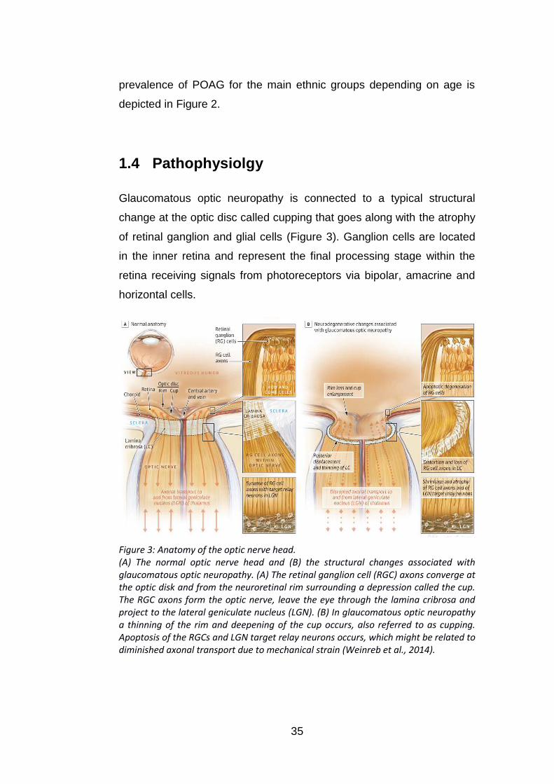
Glaucomatous optic neuropathy is connected to a typical structural
change at the optic disc called cupping that goes along with the atrophy
of retinal ganglion and glial cells (Figure 3). Ganglion cells are located
in the inner retina and represent the final processing stage within the
retina receiving signals from photoreceptors via bipolar, amacrine and
horizontal cells.
Figure 3: Anatomy of the optic nerve head. (A) The normal optic nerve head and (B) the structural changes associated with glaucomatous optic neuropathy. (A) The retinal ganglion cell (RGC) axons converge at the optic disk and from the neuroretinal rim surrounding a depression called the cup. The RGC axons form the optic nerve, leave the eye through the lamina cribrosa and project to the lateral geniculate nucleus (LGN). (B) In glaucomatous optic neuropathy a thinning of the rim and deepening of the cup occurs, also referred to as cupping. Apoptosis of the RGCs and LGN target relay neurons occurs, which might be related to diminished axonal transport due to mechanical strain (Weinreb et al., 2014).
36
Ganglion cell axon damage in glaucomatous optic neuropathy is
thought to originate at the lamina cribrosa where the axons exit the eye.
Retinal ganglion cell survival depends on neurotrophic support, which is
normally provided from their brain stem target cells and via retinal
interactions. The disrupted axonal transport causes a lower
concentration of trophic factors, which eventually leads to cell apoptosis
(Weinreb et al., 2014).
Traditionally there are two theories concerning the cause of ganglion
cell axon damage in glaucomatous optic neuropathies (Quigley, 1999).
The mechanical theory is that intraocular pressure directly impacts the
lamina cribrosa causing it to deform and restructure the lamina plates.
This also causes mechanical strain on the ganglion cell axons
eventually leading to ganglion cell death.
The vascular theory is that blood flow to ganglion cell axons at the optic
nerve head is abnormal. This in turn leads to hypoxia, a reduced
availability of oxygen or ischaemia, a reduced availability of nutrients
and oxygen. In the eye perfusion pressure is dependent on local arterial
pressure and IOP. Both raised IOP or low blood pressure may therefore
reduce blood flow (Weinreb et al., 2014).
1.5 Clinical management
1.5.1 Detection and diagnosis
Due to the typically slow progression in glaucoma, people often do not
notice a change in their vision until an advanced stage of the disease
earning it the name “the silent thief of sight”. Thus glaucoma is often
referred to as asymptomatic. An estimated number of 50% of glaucoma
cases remain undetected in developed countries (Quigley and Broman,
2006). In the UK, over 95% of referrals for suspected glaucoma are for
37
people who have visited their optometrist for a routine examination (Bell
and O'Brien, 1997b, Bell and O'Brien, 1997a).
For a diagnosis of glaucoma, typically the structure of the optic disc, the
intraocular pressure, and the visual field is examined. Gonioscopy or
imaging of the angle with optical coherence tomography (OCT) and
high resolution ultrasound permits differentiation between open-angle
and angle-closure glaucoma. The optic nerve head is typically
examined with ophthalmoscopy and imaging techniques such as OCT
and confocal laser tomography. Functional damage in the visual field is
examined with perimetry, which tests contrast sensitivity in a predefined
pattern of locations, typically within the central 30˚ of the visual field.
Due to variety in optic disc appearance and visual field test results in
the healthy population, judging a cup-disc ratio or visual field test as
abnormal is an uncertain decision. Thus there is not always a clear yes
or no diagnosis for glaucoma. Most typically both structural and
functional abnormalities have to be detectable for a clinical diagnosis of
glaucoma. However, a diagnosis of glaucoma can be made in the
absence of visual field loss, if the optic disc damage is unequivocal
(Kass et al., 2002).
1.5.2 Monitoring and treatment
Once patients have been diagnosed with glaucoma or are considered
as glaucoma suspects, they are monitored in regular visits examining
their IOP, functional and structural loss.
The general course of treatment for POAG is lowering IOP. Lowering
IOP is recommended irrespective of whether intraocular pressure is
normal (Collaborative Normal-Tension Glaucoma Study Group 1998).
For each patient a baseline IOP before treatment and an individual
target IOP is assessed. When baseline pressure is reduced by 20-40%,

38
the average rate of visual field loss progression is estimated to be
reduced by half (Jampel, 1997).
Currently, prostaglandin analogue eye drops are a first line treatment to
decrease IOP. If the target pressure is not achieved alternative eye
drops, laser treatment to the trabecular meshwork, or surgical
procedures are considered (Quigley, 2011).
39
2. The visual field
The visual field is the space a person perceives when eyes and body
are in a fixed position (Schiefer et al., 2005).
2.1 The normal visual field
The healthy visual field expands over 100˚ temporally, 70˚ inferiorly and
between 50˚ and 70˚ superiorly and nasally. The visual field extent was
first reported by Thomas Young in the 1800s and later refined by
Purkinje who used more detectable stimuli (Johnson et al., 2011). The
size of the visual field depends on each individual’s facial anatomy and
varies most nasally and superiorly depending on the shape and position
of nose and eye lid. The sensitivity throughout the visual field is not
uniform. In light-adapted conditions sensitivity is highest in the fovea –
where cone density is highest – and decreases with eccentricity of the
visual field.
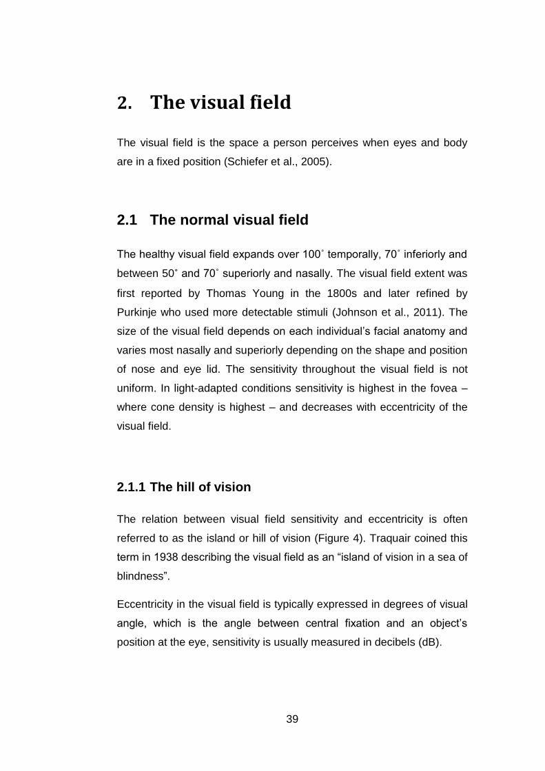
2.1.1 The hill of vision
The relation between visual field sensitivity and eccentricity is often
referred to as the island or hill of vision (Figure 4). Traquair coined this
term in 1938 describing the visual field as an “island of vision in a sea of
blindness”.
Eccentricity in the visual field is typically expressed in degrees of visual
angle, which is the angle between central fixation and an object’s
position at the eye, sensitivity is usually measured in decibels (dB).
40
The sensitivity described by the hill of vision is most typically the
contrast sensitivity, not an absolute sensitivity.
Figure 4: The island or hill of vision. The hill of vision illustrates the extent of and the contrast sensitivity throughout the visual field. Contrast sensitivity is highest at fixation and decreases with eccentricity in the visual field. The circular hole in the hill located temporally close by the horizontal meridian indicates the blind spot where the optic disc is located (Anderson, 1987).
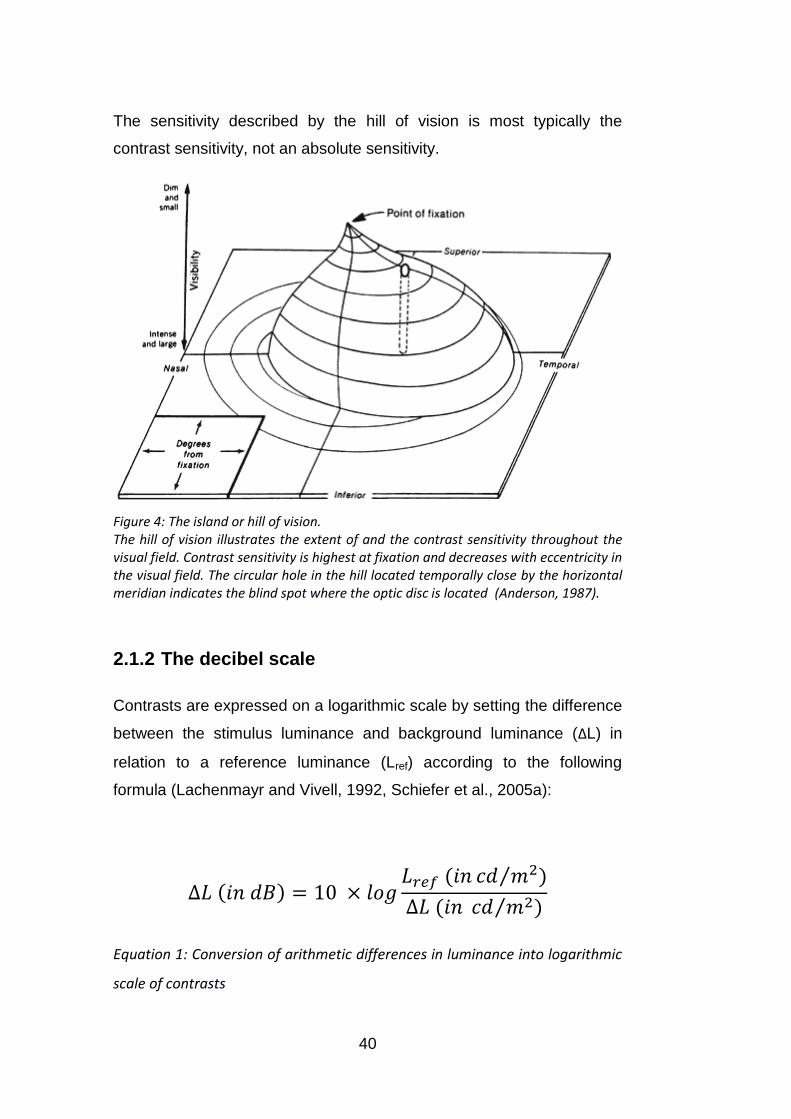
2.1.2 The decibel scale
Contrasts are expressed on a logarithmic scale by setting the difference
between the stimulus luminance and background luminance (ΔL) in
relation to a reference luminance (Lref) according to the following
formula (Lachenmayr and Vivell, 1992, Schiefer et al., 2005a):
Equation 1: Conversion of arithmetic differences in luminance into logarithmic
scale of contrasts

41
In perimetry contrast sensitivity is typically expressed in decibels (dB).
The decibel scales vary between perimeter types since the reference
luminance is chosen as the maximal stimulus luminance of the
respective instrument (Lachenmayr and Vivell, 1992, Heijl et al., 2012).
Thus 0 dB refers to the maximal stimulus luminance and lowest
measurable contrast sensitivity of an instrument and higher dB values
reflect attenuated stimulus intensities and higher contrast sensitivity.
The conversion of the decibel scale between instruments with different
maximal stimulus intensities can be easily made by adding a constant.
2.1.3 The psychometric function
The function describing the distribution of the probabilities to detect
different stimulus intensities is called the psychometric function
(Schiefer et al., 2005a, Wichmann and Hill, 2001a, Wichmann and Hill,
2001b). In a perfect observer without any false positive or negative
answers the psychometric function would be a sigmoid function with a
lower and upper asymptote at 0 and 1. In reality the false positive and
the false negative response rates determine the lower and upper
asymptote of the psychometric function respectively (see Figure 5). The
point with a 50% probability of detection determines the threshold and
the steepness of the curve indicates the response variability.

42
Figure 5: The psychometric function. Example illustrating two psychometric functions (Schiefer 2005). The x-axis gives the stimulus intensity the y-axis the probability to respond to stimuli. A response probability of 50% is defined as the threshold. The steepness of the curve indicates the response variability. The upper and lower asymptotes represent the false negative and false positive response rates, respectively. Both psychometric functions depicted have the same threshold. The slope of the red curve is steeper indicating a lower variance.
2.1.4 Factors affecting contrast sensitivity
The estimated contrast sensitivity in the healthy visual system depends
on a variety of factors. Some factors are physiological such as a decline
in sensitivity with age and variations due to media opacity in the eye,
other factors are related to the estimation technique such as stimulus
size and duration or on the constitution of the tested person, such as
attention and fatigue.
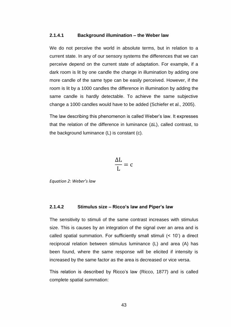
43
2.1.4.1 Background illumination – the Weber law
We do not perceive the world in absolute terms, but in relation to a
current state. In any of our sensory systems the differences that we can
perceive depend on the current state of adaptation. For example, if a
dark room is lit by one candle the change in illumination by adding one
more candle of the same type can be easily perceived. However, if the
room is lit by a 1000 candles the difference in illumination by adding the
same candle is hardly detectable. To achieve the same subjective
change a 1000 candles would have to be added (Schiefer et al., 2005).
The law describing this phenomenon is called Weber’s law. It expresses
that the relation of the difference in luminance (ΔL), called contrast, to
the background luminance (L) is constant (c).
Equation 2: Weber’s law
2.1.4.2 Stimulus size – Ricco’s law and Piper’s law
The sensitivity to stimuli of the same contrast increases with stimulus
size. This is causes by an integration of the signal over an area and is
called spatial summation. For sufficiently small stimuli (< 10’) a direct
reciprocal relation between stimulus luminance (L) and area (A) has
been found, where the same response will be elicited if intensity is
increased by the same factor as the area is decreased or vice versa.
This relation is described by Ricco’s law (Ricco, 1877) and is called
complete spatial summation:
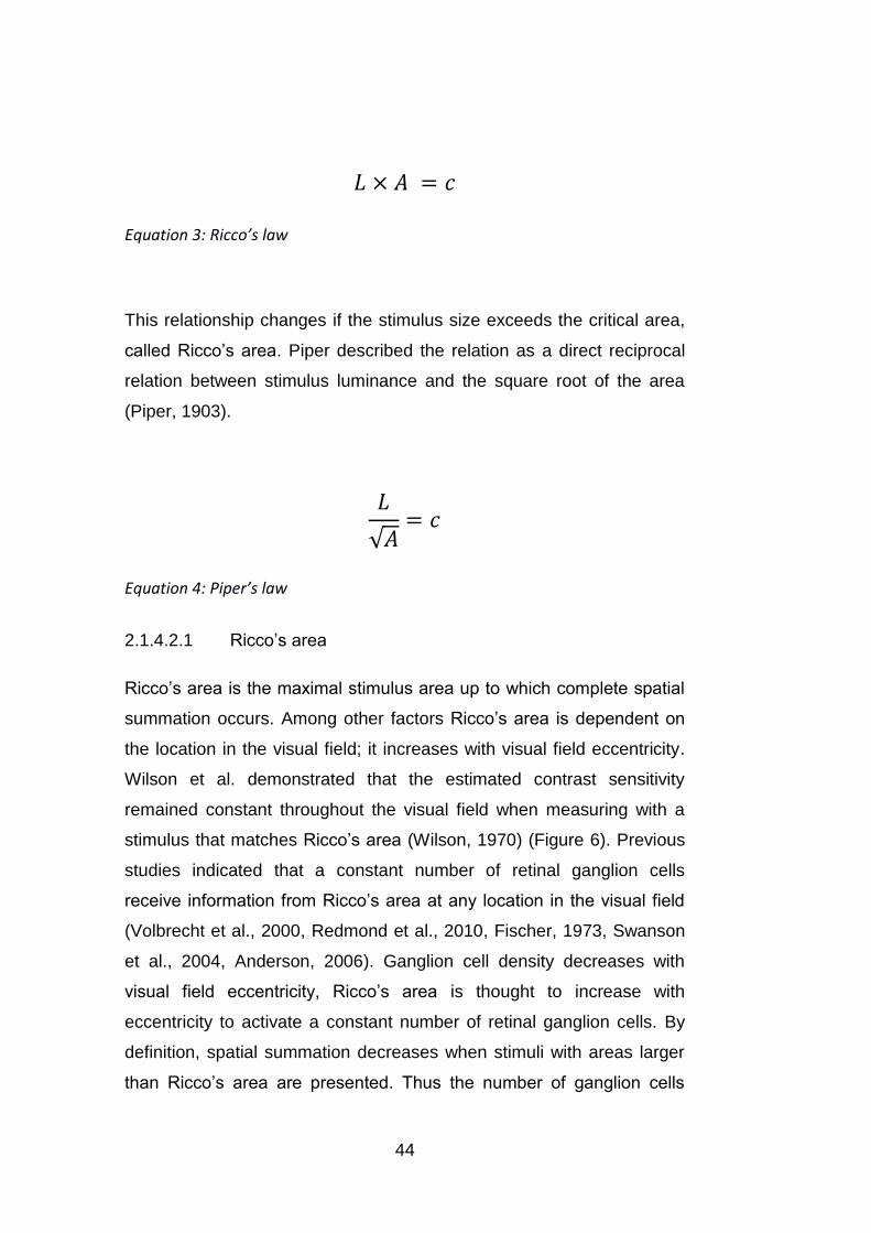
44
Equation 3: Ricco’s law
This relationship changes if the stimulus size exceeds the critical area,
called Ricco’s area. Piper described the relation as a direct reciprocal
relation between stimulus luminance and the square root of the area
(Piper, 1903).
Equation 4: Piper’s law
2.1.4.2.1 Ricco’s area
Ricco’s area is the maximal stimulus area up to which complete spatial
summation occurs. Among other factors Ricco’s area is dependent on
the location in the visual field; it increases with visual field eccentricity.
Wilson et al. demonstrated that the estimated contrast sensitivity
remained constant throughout the visual field when measuring with a
stimulus that matches Ricco’s area (Wilson, 1970) (Figure 6). Previous
studies indicated that a constant number of retinal ganglion cells
receive information from Ricco’s area at any location in the visual field
(Volbrecht et al., 2000, Redmond et al., 2010, Fischer, 1973, Swanson
et al., 2004, Anderson, 2006). Ganglion cell density decreases with
visual field eccentricity, Ricco’s area is thought to increase with
eccentricity to activate a constant number of retinal ganglion cells. By
definition, spatial summation decreases when stimuli with areas larger
than Ricco’s area are presented. Thus the number of ganglion cells

45
activated in Ricco’s area might reflect the number of cells up to which
additional activation of ganglion cells leads to a steady increase in the
neural signal and after which the signal starts to saturate. The size of
Ricco’s area has also been shown to increase in glaucoma (Redmond
et al., 2010). Glaucoma is related to a loss of retinal ganglion cells, thus
a larger stimulus area is required to activate the same number of
ganglion cells as in the equivalent region of the healthy retina.
Figure 6: Ricco’s area versus visual field eccentricity for achromatic stimuli (Anderson, 2006, Wilson, 1970). The upper plot with coloured filled circles indicates the increase in Ricco’s area diameter with eccentricity. The lower plot with unfilled black circles indicates the constancy of the contrast sensitivity ΔI/I when stimuli are matched to the localised Ricco’s area. The dotted lines indicate the eccentricity at which Goldmann stimuli (I-III) have a similar size to Ricco’s area (in the healthy visual field).
2.1.4.2.2 Goldmann stimuli
In 1945 Hans Goldmann introduced a system for perimetry stimuli that
is still widely used today (Goldmann, 1945, Gloor, 1992, Goldmann,
1999). He chose a range of stimulus sizes (sizes I-V) and contrasts

46
such that the effect of an increase from one stimulus size to the next is
equivalent to a one step increase in contrast regulated by a filter set
(filter 1-4, 5 dB steps). Notably, since Ricco’s area is dependent on
visual field eccentricity, it is questionable whether this relationship holds
in the entire visual field.
The range of Goldmann stimulus sizes is illustrated in Table 1 and the
set of filters used to attenuate stimulus contrast is described in Table 2.
Two different sets of filters to attenuate the stimulus contrast are
commonly used in Goldmann perimetry. The first set of filters (1-4)
attenuate the contrast sensitivity in steps of 5 dB from 15 to 0 dB. The
second set of filters (a-e) attenuate the contrast in steps of 1 dB from 4
to 0 dB. By combining both sets of filters a large range of stimulus
contrasts can be achieved.
Table 1: Range of Goldmann sizes with details on area in mm2 and diameter in degrees of visual angle. The area in mm2 is correct for the Goldmann perimeter with a bowl radius of 330 mm.
Goldmann sizes Area in mm2 Diameter in degrees
I
0.11˚
II 1 0.22˚
III 4 0.43˚
IV 16 0.86˚
V 64 1.72˚
Table 2: Sets of Goldmann filters used for attenuation of the stimulus contrast. The level of attenuation is given in dB.
Goldmann
Filter 1 2 3 4 a b c d E
Contrast
in dB 15 10 5 0 4 3 2 1 0

47
2.1.4.3 Stimulus duration – Bloch’s law
Contrast sensitivity also depends on the duration of the stimulus as the
visual system integrates signals over time. The maximum integration
time up to which temporal summation is present has been estimated to
lie at about 100 ms (Brindley, 1952, McDougall, 1904). For durations
below 100 ms, if stimulus luminance is increased, stimulus duration
needs to be decreased to elicit the same response (Bloch, 1885):
Equation 5: Bloch’s law
In perimetry stimulus durations typically lie between 100 and 200 ms to
avoid temporal summation and to not exceed the latency of a saccadic
eye movement (Schiefer et al., 2005a).
2.1.4.4 Observer dependent factors
With age physiological changes in the eye occur, which influence the
contrast sensitivity throughout the visual field (Spry and Johnson,
2001). The estimated decrease in contrast sensitivity per decade lies
around 0.5 dB in the central visual field and increases with eccentricity
(Heijl, 1997). Thus when interpreting the visual field age needs to be
taken into consideration to understand whether contrast sensitivity lies
within a normal range (see Chapter 3.3.3).
The visual field is determined by the individual facial anatomy. The
nasal visual field is limited by the nose and the superior visual field can
be limited by the upper eye lid. Droopy eyelids can be taped to prevent
artefacts in the superior visual field that might be misinterpreted as

48
visual field defects. Refractive errors can also diminish contrast
sensitivity. Thus an appropriate refractive correction that is adjusted to
the distance at which stimuli are presented is essential to measure the
visual field (Lachenmayr and Vivell, 1992, Heijl et al., 2012). The pupil
size can influence contrast sensitivity as it determines the amount of
light that can enter the eye. The pupil should have a diameter of at least
2 mm to prevent artefacts in visual field measures (Mikelberg et al.,
1987, Lachenmayr and Vivell, 1992).
While factors such as droopy eye lids, refractive errors or small pupil
size can be accounted for by ensuring that they are handled
appropriately, other factors are more difficult to control. Increased
medium opacity, as for example caused by cataract, leads to reduced
light levels at the retina and scattering of the light that enters the eye.
This can cause an effect in visual field results that looks similar to
diffuse visual field loss as it can occur in glaucoma (see Chapter 2.2.1).
Thus measuring medium opacity can help to interpret visual field results
correctly (Lachenmayr and Vivell, 1992).
Psychological factors of the examined person also affect the estimation
of contrast sensitivity. Fatigue or low attentional capacities can lead to
high false positive or false negative response rates that introduce noise
and result in imprecise estimates of contrast sensitivity. Learning effects
can play a role during the first visual field examinations. Low contrast
sensitivities might be related to an unfamiliarity with the task and
disappear during repeated examinations. False negative and false
positive response rates are often estimated in automated visual field
examinations (see Chapter 3.3.2) as indicators for test reliability.

49
2.2 Visual field damage in glaucoma
Functional loss in glaucoma to date is irreversible. Typically visual field
loss progresses slowly and people are often unaware of it until more
advanced stages. Glaucomatous visual field loss is usually bilateral, but
mostly asymmetric between eyes. On average, one eye presents with
twice as much damage as the other eye (Quigley, 2011, Broman et al.,
2008). Typically the deterioration of the visual field begins in the mid-
periphery and often progresses in a centripetal manner (Weinreb et al.,
2014). Only up to 15% of patients with glaucoma were found to present
with early damage in the far periphery (LeBlanc and Becker, 1971).
Central and far peripheral areas of the visual field are mostly affected at
a later stage of the disease. A variety of visual field loss patterns have
been described in glaucoma.
2.2.1 Diffuse visual field loss
Diffuse visual field loss describes a relatively uniform reduction in
sensitivity loss throughout the entire or a large portion of the visual field.
Henson et al. reported diffuse loss to be present in the most sensitive
region of the central visual field in most cases of early glaucoma
(Henson et al., 1999). However, the prevalence of diffuse loss in
glaucoma is a controversial topic. Since smaller regions with uniform
low sensitivity loss are often referred to as diffuse loss, the same region
might be classified as a localised loss at a later stage with deepening of
the scotoma (Mutlukan, 1995). Additionally generalised sensitivity loss
often might not be indicative of glaucomatous loss but rather of an
uncorrected refractive error or increased media opacity (Brusini, 1997).

50
2.2.2 Localised visual field loss
Localised visual field defects have been found to most likely occur in
the superior hemifield and the inferior nasal quadrant (Henson and
Chauhan, 1985, Henson and Hobley, 1986). First defects often start out
in the paracentral region called paracentral scotoma (Figure 7e). These
are independent of the blind spot (Drance, 1969). Paracentral scotoma
often progress by joining with the blind spot in a circular manner (Figure
7c, f). The form of this arc-shaped defect called arcuate scotoma or
Bjerrum scotoma (Harrington, 1964) closely resembles the arcuate path
of the retinal nerve fibers to the optic nerve. In later stages of glaucoma
inferior and superior arcuate defects often merge resulting in a ring
scotoma. Other localised defects described in glaucoma are an
enlargement of the blind spot (Drance, 1969) and the so called nasal
step (Figure 7a, c, f). The nasal step is an asymmetric nasal defect at
the border between inferior and superior quadrant, which is reflected in
a step-like appearance in kinetic perimetry. Examples of typical
glaucomatous visual field defects can be seen in Figure 7.
Figure 7: Various types of glaucomatous visual field defects as found with static perimetry of the central 30˚ of the visual field (Broadway, 2012).

51
3. Perimetry
Perimetry is the examination of a person’s visual field. Conventional
perimetry seeks to estimate contrast sensitivity throughout the visual
field. This is typically done in one of two ways: either by moving stimuli
from less sensitive towards more sensitive areas recording the point of
detection, called kinetic perimetry, or by presenting stimuli of different
contrast in the same location and recording detection, called static
perimetry.
3.1 A brief history of perimetry
This section reviews some of the highlights in the history of perimetry.
There are a number of reviews giving detailed accounts (Johnson et al.,
2011, Lachenmayr, 1988, Draeger and Hendriock, 1998, Thompson
and Wall, 2008).
The examination of our visual field has a long history, one of the first
recorded accounts of the evaluation of the peripheral visual field was
from Hippocrates in the late fifth century B.C. (Johnson et al., 2011).
First illustrations of the visual field stem from Ulmus published in 1602.
The blind spot was first described by Mariotte in 1668, who also related
it to the location of the optic disc (Johnson et al., 2011, Berens, 1923,
Justel and Mariotte, 1668). In the early 1800s Thomas Young measured
the extent of a normal visual field (Thompson and Wall, 2008, Johnson
et al., 2011). The step from qualitative to quantitative perimetry was
performed by Albrecht von Graefe inspired by Helmholtz’
recommendation to guide the fixation (Johnson et al., 2011). Von
Graefe introduced a screen with a fixation target and used a fixed
examination distance (Thompson and Wall, 2008, Johnson et al., 2011).
Visual field examinations that are performed on flat surfaces for
stimulus presentations are often referred to as campimetry. One of the

52
best known further developments of such a screen is the tangent
screen by Jannik Bjerrum, also referred to as Bjerrum screen (Johnson
et al., 2011).
A major step towards modern day perimetry was the work of Hans
Goldmann in the 1940s (Goldmann, 1999, Goldmann, 1945). The
largest contribution of Goldmann perimetry was its drive towards
standardisation. Building on the work of Ferree and Rand (Ferree and
Rand, 1930a, Ferree et al., 1926, Ferree et al., 1930b, Ferree et al.,
1931b, Ferree et al., 1929), Goldmann designed a bowl perimeter with
a uniform background illumination, a set of standard stimulus sizes and
a set of filters to regulate the stimulus contrast. Goldmann furthermore
standardised the charts for visual field recording and ensured a precise
recording through the use of a pantograph that simultaneously guided
the stimulus presentation and the recording of the examinee’s
responses.
In the age of computerization the next logical step was an automation of
perimetry. The pioneers in the automation of perimetry were F.
Fankhauser, J. Lynn, A. Heijl, C.E.T. Krakau and S. Drance
(Fankhauser et al., 1972, Fankhauser et al., 1977, Lynn and GW, 1972,
Heijl and Krakau, 1975b, Heijl and Krakau, 1975a, Heijl et al., 1980,
Thompson and Wall, 2008). The automation of perimetry focused
mainly on static perimetry. Computer based perimetry allowed an easy
use of adaptive techniques to determine detection thresholds in specific
locations of the visual field (Johnson et al., 1992). Over time the
efficiency of these techniques has been further refined from simple
staircase methods to more complex strategies e.g. including Bayesian
priors (Schiefer et al., 2009, Bengtsson and Heijl, 1998a, Bengtsson et
al., 1998, Bengtsson et al., 1997).
In the last decades alternative perimetric techniques such as short
wavelength automated perimetry (SWAP) (Heron et al., 1988) or
frequency-doubling perimetry (Johnson and Samuels, 1997) have been

53
suggested that focus mostly on early detection of glaucoma by tapping
into different visual pathways (Anderson, 2006).
3.2 Statistical properties of threshold estimates
Clinical perimetry needs to yield reliable threshold estimates, yet be
time efficient.
An optimal threshold estimate would be robust against patient errors,
accurate – which means the absence of bias, precise – which means
the absence of variance, and efficient – which means needing a
minimal number of stimulus presentations to reach precision.
The bias is the difference of the average estimated threshold from the
true threshold. Since the true threshold can never be known with real
observers, the bias can only be derived from simulations.
Precision is the inverse of the variance of the threshold estimates. A
distribution of threshold estimates with high variance around a mean at
the true value is imprecise but accurate. A distribution of threshold
estimates with low variance around a mean that differs from the true
value is precise but inaccurate.
3.3 Static automated perimetry
Since the introduction of computer supported static perimetry
(Fankhauser et al., 1972, Fankhauser et al., 1977, Lynn and GW, 1972,
Heijl and Krakau, 1975b, Heijl and Krakau, 1975a, Heijl et al., 1980),
automated static perimetry has been established as a standard in
clinics for patients with glaucoma. Static automated perimetry most
typically uses constant stimulus sizes and durations while varying
stimulus contrast to estimate the detection threshold. The locations are

54
often fixed to predefined patterns. Some of the most commonly used
test patterns are the 30-2, the 24-2, the G1 (Zulauf et al., 1994, Zulauf,
1994) and the 10-2 pattern, consisting of grids with 76, 54, 73 and 68
locations respectively (see Figure 8).
Figure 8: Visual field test patterns. The graph on the left depicts the 30-2 pattern (all dots) compared to the 24-2 pattern (dots in blue)(Heijl and Patella, 2002). The middle graph shows the 10-2 pattern (red dots) compared to the 24-2 pattern (blue dots)(Heijl et al., 2012). The graph on the right represents the G1 pattern (Schiefer et al., 2006b).
These test patterns can be used for suprathreshold or threshold
perimetry. Most commonly thresholds are estimated in each location.
Threshold perimetry is often referred to as standard or static automated
perimetry.
3.3.1 Threshold estimation procedures
3.3.1.1 Method of constant stimuli
One of the most accurate threshold estimation techniques is the method
of constant stimuli (Spearman, 1908, Urban, 1910, Treutwein, 1995).
Here, stimuli with different intensities spanning a range from detectable
to non-detectable are presented in randomised order, and the intensity
corresponding to the 50% point of detection is determined as the
threshold. However, this technique needs a large number of stimulus
presentations to get a fair estimate of the threshold and is thus too time-
consuming for clinical perimetry.

55
3.3.1.2 Adaptive procedures
In adaptive procedures stimulus values depend on previous responses
(Treutwein, 1995, Falmagne, 1986).
The staircase method changes stimulus intensity by a certain step size
depending on the response to previous stimuli. A stimulus that is
detected would be attenuated by the specified step size in the next
presentation until it is not seen anymore. The change from seen to not
seen, or from not seen to seen, is referred to as a reversal, which then
results in a change in the direction of attenuation typically with a smaller
step size. The staircase method terminates after a certain number of
reversals. Staircase methods tend to yield less precise threshold
estimates than the method of constant stimuli, they are however less
time consuming and thus more suitable for clinical perimetry.
Bayesian and maximum likelihood procedures appear similar to
staircase methods to the observer but differ profoundly in the estimation
technique of the threshold (Treutwein, 1995, Bengtsson et al., 1997). In
maximum likelihood techniques the threshold is calculated based on all
previous responses. Bayesian procedures include a prior likelihood in
the estimation. Bayesian procedures can be more efficient than
staircase methods however they are also more prone to bias than
staircase methods and the method of constant stimuli.
3.3.2 Threshold estimation strategies in perimetry
Various versions of adaptive procedures, such as full threshold and
SITA standard on Humphrey perimeters (Carl Zeiss Meditec., Inc.,
Dublin, CA) and GATE and TOP on the Octopus 900 (Haag-Streit,
Köniz, Switzerland), have been established in clinical perimetry, each
aiming for an efficient trade off between test time, accuracy and
precision of the threshold estimation.
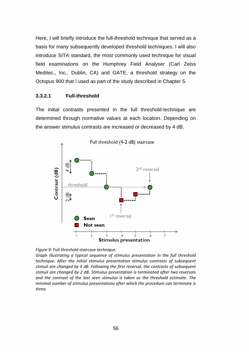
56
Here, I will briefly introduce the full-threshold technique that served as a
basis for many subsequently developed threshold techniques. I will also
introduce SITA standard, the most commonly used technique for visual
field examinations on the Humphrey Field Analyser (Carl Zeiss
Meditec., Inc., Dublin, CA) and GATE, a threshold strategy on the
Octopus 900 that I used as part of the study described in Chapter 5.
3.3.2.1 Full-threshold
The initial contrasts presented in the full threshold-technique are
determined through normative values at each location. Depending on
the answer stimulus contrasts are increased or decreased by 4 dB.
Figure 9: Full threshold staircase technique. Graph illustrating a typical sequence of stimulus presentation in the full threshold technique. After the initial stimulus presentation stimulus contrasts of subsequent stimuli are changed by 4 dB. Following the first reversal, the contrasts of subsequent stimuli are changed by 2 dB. Stimulus presentation is terminated after two reversals and the contrast of the last seen stimulus is taken as the threshold estimate. The minimal number of stimulus presentations after which the procedure can terminate is three.

57
After the first reversal the step size changes to 2 dB (4-2 dB staircase).
The stimulus presentation terminates after two reversals. The contrast
of the last detected stimulus determines the final threshold estimate
(Artes et al., 2002). A typical sequence of stimulus presentations for
threshold determination with the full-threshold technique is illustrated in
Figure 9.
3.3.2.2 SITA Standard
SITA Standard combines a 4-2 dB staircase method with a maximum
likelihood procedure for estimating thresholds.
The SITA strategy is approximately twice as fast as the full threshold
strategy. This reduction in time is achieved through the following
adjustments: A more efficient threshold estimation strategy; an
estimation of false positives through responses outside expected
response times, which eliminates catch trials; an adjustment of the
interstimulus interval to individual response times; and repeated
threshold estimation only from points where initial estimates differ from
expected values by more than 12 dB, instead of 4 dB as in the full
threshold strategy (Turpin et al., 2003).
The first four test locations, called primary locations, are estimated with
the full threshold strategy. Based on their thresholds the initial values
for other test locations are calculated. As prior knowledge SITA uses a
model incorporating distributions of age-corrected normal thresholds at
each test point, frequency-of-seeing curves and correlations between
threshold values at different test locations. The prior model consists of
two prior likelihood functions, one for normal, one for abnormal points,
describing the probability for estimated threshold values at each
location. The model is updated with each response and eventually the
maximum posterior estimate is chosen as the threshold estimate
(Bengtsson et al., 1997).

58
3.3.2.3 GATE
The German Adaptive Threshold Estimation (GATE) strategy uses a
modified 4-2 dB staircase terminating after two reversals (Schiefer et
al., 2009, Luithardt et al., 2015). At the outset of the initial test,
thresholds are determined at four “seed” locations. Start contrasts at
other locations are dependent on the thresholds at seed locations.
Subsequent start contrasts are suprathreshold to previous test results.
In contrast to the full threshold strategy, a non-seen initial stimulus is
followed by a stimulus at 0 dB (maximum intensity). If this stimulus is
not detected the procedure terminates, otherwise a stimulus 4 dB
brighter than the initial intensity is presented. The contrast midway
between the brightest stimulus not seen and dimmest stimulus seen is
chosen as the threshold estimate.
3.3.3 Interpretation of test results
Perimetry is frequently performed to find whether a single visual field
result or the change in a series of visual fields of the same patient is
within or outside normal limits in the respective age group. The change
in sensitivity with age in healthy subjects appears to be linear
throughout the visual field (Heijl et al., 1987). However, the rate of
visual field change seems to get steeper with eccentricity, which results
in a depressed and steeper hill of vision with age.
The response variability and retest variability of threshold estimates
depends on the location within the visual field. Heijl et al. found
variability to increase with eccentricity (Heijl et al., 1987). This increase
with eccentricity appears to be related to the decrease in contrast
sensitivity with visual field eccentricity (Henson et al., 2000) and holds
true for inter-subject variability, intra-subject (test-retest) variability
(Russell et al., 2012a, Artes et al., 2002), as well as intra-test variability

59
(Henson et al., 2000). Thus a given deviation from the normal average
could be clinically significant in the central, but not in the peripheral
visual field.
On Humphrey perimeters the package STATPAC provides a series of
analyses evaluating the test reliability and deviation from normal.
Raw test results:
On a typical printout threshold estimates are represented as numbers
and as a greyscale. The maximal stimulus contrast is 0 dB, which is
represented as black in the greyscale and reflects areas with lowest
sensitivity. Higher sensitivities are represented in lighter shades of grey.
Contrast sensitivities – even in young subjects – typically do not exceed
40 dB (Heijl et al., 2012).
Probability plots:
Total deviation probability plots give the deviation from age-corrected
normal values at each test point. Since the normal range of sensitivities
increases with eccentricity, the same total deviation might be clinically
significant in a central position, but not further in the periphery (Heijl et
al., 1987). The degree of the deviation from a healthy reference group is
indicated for sensitivities that are worse than the 5th, 2nd, 1st and 0.5th
percentile of the healthy reference group.
By correcting for generalised depression, the pattern deviation
probability plots highlight localised visual field defects. In very advanced
field loss (mean deviation worse than -15 dB) pattern deviation plots
become unreliable because diffuse and generalised loss can no longer
be distinguished from each other.
Global Indices:
Two widely used summary measures for static visual fields are mean
deviation (MD) and pattern standard deviation (PSD), which is referred

60
to as “loss variance” on Octopus perimeters (Tonagel et al., 2012). The
MD indicates how much the whole field differs on average from a
healthy reference group. It is a weighted average of the deviations
shown in the total deviation plot (Heijl et al., 2012). The PSD indicates
local irregularities in the visual field. It is the standard deviation of the
total deviations. Deep local defects result in higher PSD values than
diffuse loss (Tonagel et al., 2012, Heijl et al., 2012). Compared to
probability maps, global indices are less useful for diagnostic purposes;
they can be within normal limits when visual field loss is clearly present
(Heijl and Patella, Essential Perimetry).
Glaucoma Hemifield Test (GHT):
The Glaucoma Hemifield Test is an analysis based on the finding that
glaucomatous loss often occurs asymmetrically in the inferior and
superior hemifield. It directly compares pattern deviation probability
values of five zones above the horizontal midline with five mirror image
zones below the midline. The visual field printout indicates significantly
different results in one or more of the upper regions from the
corresponding lower regions as “Outside Normal Limits” at a p-value <
0.01 and as “Borderline” at a p-value <0.03 (Åsman and Heijl, 1992,
Heijl et al., 2012).
Reliability indices:
False positive (FP) rates indicate how prone a patient is to respond in
the absence of a stimulus. False positive response rates are typically
estimated by either introducing catch trials during which the perimeter
produces the usual sounds, but no detectable stimulus is presented or
by monitoring the number of responses occurring implausibly early after
a presentation. A high number of false positive responses can
adulterate test results and lead to unusually high threshold estimates.
False negative (FN) rates are typically estimated by presenting supra-
threshold stimuli at already measured test locations. The interpretation
61
of false negative rates needs to be treated carefully as a high response
variability, as present for example in defective areas, can lead to an
overestimation of the FN rate.
Fixation loss rates are normally estimated by presenting stimuli with
maximal contrast in the blind spot region. Some instruments additionally
monitor fixation via a gaze tracker.
3.3.4 Suprathreshold perimetry
Suprathreshold perimetry does not aim to estimate the threshold, but to
indicate whether sensitivity is abnormally low in any location of the
visual field. It is often referred to as a screening test. Suprathreshold
perimetry is faster than threshold perimetry since there is typically only
one stimulus presentation with an above-threshold stimulus at each
location. While suprathreshold perimetry might indicate some visual
field defects it has been criticised to be insensitive for early
glaucomatous loss (Mills et al., 1994).
3.4 Kinetic perimetry
In kinetic perimetry stimuli, typically with constant area and contrast, are
moved across the visual field. The direction of movement is from areas
with lower to higher expected sensitivity, thus from “non-seeing” to
“seeing”. The locations at which stimuli are first seen are recorded.
The standard background illumination used in kinetic perimetry was
established by the Goldmann perimeter and lies at 10 cd/m2 (31.4 asb).
This adaptation level approximates to the minimal brightness for
photopic vision that depends more on cone than on rod function (Heijl et
al., 2012). The slope of the hill of vision flattens with lower background
illumination (see Figure 10), which has an impact on the variability of

62
kinetic perimetry. In contrast to static perimetry, thresholds in kinetic
perimetry are mapped by moving stimuli horizontally across the hill of
vision. Thus the steepness of the hill of vision particularly influences the
variability of responses. If the stimulus is moved across a steep hill of
vision the contrast sensitivity of neighbouring locations changes rapidly.
Thus the area within which a stimulus is likely to be detected is small.
However with a shallow hill of vision the contrast sensitivity is similar
over a wider space, thus locations of detection for a stimulus with the
corresponding contrast might be widely spread, leading to higher
response variability.
Figure 10: Representation of background lighting effect on the hill of vision (Calixto et al., 2006). The hill of vision flattens with lower background illumination. As kinetic stimuli are moved horizontally across the hill of vision, its steepness affects the variability of the detection threshold. With a flatter hill of vision responses are more likely to be spread over a larger area.
In kinetic perimetry, locations at which the same stimulus intensity is
detected are connected to an isopter. Similar to contour lines in
cartography that indicate regions of equal elevation on a map, isopters
indicate regions of the same contrast sensitivity in the visual field. Due
to the form of the normal hill of vision, isopters have elliptic shapes.
Distortions from this shape can indicate areas of visual field loss.

63
For a complete examination of the visual field stimuli with different
intensities are presented to map out several isopters. The stimulus
intensity is adjusted by either changing the stimulus size or the stimulus
contrast, or both. Typically, stimuli are moved at speeds ranging from 1-
5˚ per second (Schiefer et al., 2005b, Lachenmayr and Vivell, 1992,
Goldmann, 1945). The choice of the stimulus velocity can depend on
the expected eccentricity of an isopter. In the central visual field a
slower motion of the stimuli is recommended (1˚-2˚/second), and faster
motion in the periphery (2˚-5˚/second) (Schiefer et al., 2005b,
Lachenmayr and Vivell, 1992, Goldmann, 1945, Vonthein et al., 2007,
Johnson and Keltner, 1987).
3.4.1 Kinetic test strategies
3.4.1.1 Goldmann manual kinetic perimetry
The development of Goldmann’s bowl perimeter was an important step
in the standardisation of quantitative perimetry as it provided a uniform
background illumination and standardised stimuli (Goldmann, 1945)
(Goldmann, 1999). The Goldmann perimeter (Figure 11) allows the
examiner to monitor fixation, adjust background illumination and control
stimulus size and contrast via a set of standardised filters. (The range of
Goldmann stimuli is described in Chapter 2.1.4.2.2, page 45). Notably,
the range of stimulus sizes and contrast increments were chosen such
that a gain in visual sensitivity at a certain location in the visual field
caused by an increase of one step size of stimulus area was equivalent
to that caused by an increase of one step size in contrast of one of the
filters. The visual field is recorded on standardised charts (Figure 12)
using a pantograph, which guides the stimulus presentation (Figure 11).

64
Figure 11: The Goldmann Perimeter. Left: side facing the patient with chin rest and hemispherical bowl . Right: side facing the examiner with pantograph for stimulus guidance and chart for visual field mapping (Pollack-Rundle).
Figure 12: Goldmann visual field chart. Isopters are drawn for a person with healthy vision from a typical examination with Goldmann perimetry (Haag-Streit-International).
In a typical clinical examination, each eye is tested individually.
Corrective lenses are used for the examination within the central 30˚

65
only. In general stimuli are moved from non-seeing towards seeing
areas at a speed around 5˚ per second.
According to the Goldmann perimeter manual (Haag-Streit-
International) an examination is started with a I4e stimulus, followed by
mapping a I3e, I2e and I1e isopter. If two isopters are too widely spaced
an additional greyscale filter is introduced to achieve an intermediate
stimulus intensity. The blind spot is examined with the stimulus of the
isopter including the blind spot region. Normally 8-12 vectors at every
30-45˚ are sufficient to map a single isopter. If a local abnormality is
detected, additional test vectors are introduced. Scotomas are mapped
by moving the stimulus perpendicularly to the expected isopter.
Goldmann perimetry has remained mostly unchanged and is still used
in clinics. More recent guidelines for kinetic perimetry suggest using the
III4e stimulus for the initial isopter or choosing the initial stimulus
depending on the subject’s visual acuity (Pollack-Rundle, Haag-Streit-
AG, 2013). Furthermore the blind spot is typically mapped with a I4e
stimulus. Since asymmetrical defects along the horizontal meridian,
such as the nasal step, are common in glaucoma, additional test
vectors temporally and nasally above and below the horizontal meridian
are often introduced for glaucoma examinations.
For a more thorough examination of the central 30˚, an additional static
examination following the Armaly-Drance technique can be performed
on the Goldmann perimeter (Rock et al., 1973, Armaly, 1971, Stewart
and Shields, 1991). The static examination consists of 76 test locations
and suprathrehold stimuli are presented at each location. Locations
marked as non-seen are usually rechecked with increasing stimulus
intensity. If the V4e stimulus is not detected the location is marked as
an absolute scotoma (Pollack-Rundle).
Manual kinetic perimetry requires well trained examiners and depends
on the examiner’s judgement.

66
3.4.1.1 Semi-automated and automated kinetic perimetry
Semi-automated and automated kinetic perimetry eliminates most of the
examiner dependence of manual Goldmann perimetry. Target speed
can be kept constant and a more accurate estimation of response times
is possible.
Semi-automated kinetic perimetry is available on the Octopus 900 by
Haag-Streit (Koeniz, Switzerland) (Figure 13). Kinetic visual field
examinations similar to Goldmann perimetry can be performed on the
Octopus 900 as it provides the same range of stimuli (Haag-Streit-AG,
2013).
Figure 13: The Octopus 900 (Haag-Streit, Koeniz, Switzerland). The chin rest is adjustable and the gaze is monitored through a camera (small screen on the perimeter). Perimetric examinations are run via the EyeSuite software on an external computer (Haag-Streit, 2014).
Additionally to semi-automated perimetry, the EyeSuite software allows
the user to customise basic automated tests for the Octopus 900.
No standard automated kinetic examination has been established to
date. However, different versions of automated kinetic perimetry have
been suggested. Johnson et al. designed an algorithm for stimulus

67
presentation that first determined the set of stimuli appropriate for the
individual patient during an exploratory scan along four meridians
(Johnson et al., 1987). A first scan was then performed along twelve
meridians. Stimulus presentations were repeated where isopter
locations fell outside of an age-matched normal range. The Allergan-
Humphrey Visual Field Analyser also provides an approach for
technician-assisted automated kinetic perimetry (Lynn et al., 1990). The
technique evaluates the visual field along 28 meridians, isopter
locations are determined with one stimulus presentation along each
meridian. An evaluation of the technique showed that spurious
responses lead to spikes in the isopter form in 80% of visual field
examinations (Lynn et al., 1990). Matsumoto et al.’s Program K
overcomes this problem and is a promising attempt to simulate the
typical decision making of a trained examiner in Goldmann perimetry in
an automated test (Wakayama et al., 2011, Hashimoto et al., 2012,
Hashimoto et al., 2015). Their algorithm accepts isopter locations after
one stimulus presentation if the response is within an expected normal
range at that location. If abnormal responses occur, additional stimuli
are presented along the same meridian. To map abnormal regions in
more detail additional test points are also introduced next to abnormal
isopter locations. The additional stimuli are moved perpendicularly to
the previously estimated isopter border. Another promising idea is the
combination of static automated perimetry of the central visual field with
the kinetic automated examination of peripheral isopters (Pineles et al.,
2006).
Automated kinetic perimetry holds the advantage to allow better
comparability between examinations due to more standardised test
procedures and digitalised data. The automation of kinetic perimetry
permits to establish normative isopter values (Vonthein et al., 2007) and
standardised analyses for test results of kinetic perimetry.

68
3.4.2 Interpretation of test results
There are no standard automated analyses of kinetic test results
comparable to the StatPac package (evaluation of static perimetry).
Instead results are mostly evaluated by eye or by customised programs.
For diagnostic purposes visual field results are typically compared
against normative values of healthy participants. The semi-automated
kinetic perimetry program on the Octopus 900 plots estimated isopters
against normative regions (Haag-Streit-AG, 2013). Variations from
normal, in the form of a general constriction of an isopter or a local
depression in an isopter, indicate abnormalities in the visual field. The
choice of summary measures, which indicate the size of isopters, varies
between studies (Christoforidis, 2011, Nevalainen et al., 2008). Most
commonly the isopter area is used as a summary measure (Nevalainen
et al., 2008, Nowomiejska et al., 2005, Ramirez et al., 2008). However,
the choice of units is not uniform throughout studies. The isopter area is
for example described in square degrees of visual angle in some
studies (Nevalainen et al., 2008, Nowomiejska et al., 2005) and in cm2
on a standard chart in other studies (Ramirez et al., 2008). An
alternative suggested measure taking contrast sensitivity in account as
a third dimension is visual field volume (Christoforidis, 2011). This
provides the advantage of allowing a comparison with static perimetry
results when applying the same calculation to static test results.
With recent efforts to automate kinetic perimetry, kinetic perimetry test
results are more closely examined aiming to evaluate variability of
responses to kinetic stimuli and to establish normative isopter values. A
model for estimating normative isopter values depending on patient age
and stimulus parameters based on semi-automated kinetic perimetry in
participants with healthy vision has been proposed by Vonthein and
colleagues (Vonthein et al., 2007). Kinetic perimetry was found to yield
reproducible results (Hirasawa and Shoji, 2014, Parrish et al., 1984,
Nevalainen et al., 2008, Nowomiejska et al., 2012, Bjerre et al., 2014).

69
Furthermore, test results from Goldmann manual perimetry and semi-
automated kinetic perimetry appear to be similar (Nowomiejska et al.,
2005, Ramirez et al., 2008, Rowe and Rowlands, 2014). Visual field
results from kinetic perimetry were found to add clinically relevant
information to visual field results from static automated perimetry of the
central 30˚ (Ballon et al., 1992, Miller et al., 1989, Nowomiejska et al.,
2014).
3.5 Practical application of static and kinetic
perimetry
3.5.1 Statokinetic dissociation
Having two different techniques to examine the visual field poses the
question how results of these examinations relate. Kinetic perimetry
keeps stimulus size and contrast constant and has visual field location
as its variable, static perimetry keeps the location and stimulus size
constant and uses stimulus contrast as its variable. Thus kinetic
perimetry results describe locations in degree of visual angle while
static perimetry results are detection thresholds in dB. In principle, both
techniques relate points in the visual field with contrast sensitivity.
However, the sensitivity to a moving versus a static stimulus appears to
differ. Riddoch et al. coined the term statokinetic dissociation,
describing the phenomenon that sensitivity appears to be higher to
moving than to static stimuli (Riddoch, 1917). This finding was
corroborated by various studies comparing static thresholds to locations
determined with kinetic stimuli (Safran and Glaser, 1980, Hudson and
Wild, 1992, Schiller et al., 2004). Hudson and Wild found sensitivity to a
range of kinetic Goldmann stimuli to be on average 4 dB higher than to
static stimuli. Within the range of stimuli they used this appeared to be
largely independent of age, eccentricity, stimulus size and meridian.

70
The exact cause for the difference in sensitivity is unknown. An
intrinsically higher sensitivity to motion by certain ganglion cell types
could be part of the explanation. However, it is unclear as to how far
differences in the two techniques contribute to the dissociation. The
kinetic stimulus can travel over a wide area of the retina until it is
detected. Responses of retinal ganglion cells that are not sufficient to
lead to a conscious percept of the stimulus might still contribute to the
later signal. Furthermore, the duration for which a stimulus is exposed
to receptive fields of retinal ganglion cells is likely to differ between
static and kinetic stimuli. Moreover, the response criterion of individual
patients could influence statokinetic dissociation. As kinetic stimuli are
likely to be detected at some point in the visual field, patients might tend
to choose more conservative response criteria.
3.5.2 Examination of the central versus peripheral visual
field
With the development of standard automated perimetry, the main focus
was directed to the central 30˚ of the visual field (Stewart and Shields,
1991). Since manual Goldmann perimetry requires well trained staff and
longer test durations, it is used less and less in clinics. It is, however,
unclear how much information is lost by not examining beyond 30˚.
Both kinetic and static perimetry allow examining large proportions of
the visual field. Test patterns for static perimetry going further in the
periphery are available, such as the 60-2 pattern on the Humphrey
perimeter and Program 07 on the Octopus 900, and using low intensity
stimulus parameters allows kinetic examination of the central visual
field. However, while SAP appears to be efficient for the central visual
field, static perimetry might require too many test locations for a good
resolution in the peripheral visual field. Which technique is more
efficient for examining the peripheral visual field needs further

71
investigation. A combined automated approach using static perimetry
for the central 30˚, and kinetic perimetry for the visual field beyond this
area (Pineles et al., 2006, Miller et al., 1989) might be useful to examine
the entire visual field. In late stage glaucoma, often only a central (close
to fixation) and peripheral island remain (Scheuerle et al., 2012,
Nowomiejska et al., 2014). In such cases a static macular examination
combined with a kinetic examination of the peripheral visual field might
be more suitable and less frustrating for the patient.

72
4. Visual disability in glaucoma
The human being is a visual being. We rely on our sense of vision when
navigating, remember visual landmarks for our orientation, use traffic
signs to communicate rules, use graphs to visualise complex statistics,
have a written visual representation of our language and a large part of
our communication is based on visual cues through gestures and facial
expressions. Even having lost our sense of vision, the neural capacities
of the visual cortex still help us to perform extraordinary tasks. As such,
fMRI and TMS studies showed that the primary visual cortex is involved
in Braille reading in the blind (Burton et al., 2002, Ptito et al., 2008).
Losing our ability to see makes it difficult or even impossible to perform
many tasks of our everyday life, can isolate us and reduce participation
in society.
The aim of this short chapter is to briefly outline some aspects of visual
disability that result from glaucomatous visual field loss. The focus here
is to highlight aspects of visual function that would be better measured
by a test that would measure the visual field in the far-periphery. After
all, this would be a strong motivation for developing such a test. This
section considers the impact of visual field loss on driving, reading and
mobility. The latter is most likely to benefit from a better assessment of
the peripheral visual field when compared to what is clinically used at
the moment.
Section 4.3 (Mobility, balance and risk of falling) of this chapter formed
part of a review published in the International Journal of Ophthalmic
Practice (Moenter et al., 2014).
Impairment is defined as: “any loss or abnormality of psychological,
physiological, or anatomical structure or function” (World-Health-
Organization, 1980). In contrast the term disability entails: “a restriction
or lack of ability to perform an activity in the manner or within the range

73
considered normal for a human being” (World-Health-Organization,
1980). Thus, the presence of impairment does not necessarily imply
that a person’s everyday life is affected while the presence of a
disability does. In the context of this thesis, a person may have visual
impairment because they have a scotoma in their peripheral visual field.
This impairment only leads to visual disability if it impacts on that
person’s everyday life. For instance, a person with central or peripheral
visual field loss may have difficulty locating objects or finding the next
line of print in a book they are reading. More visually disabling could be
problems navigating around a room or difficulty with driving – such
disabilities could have greater impact because they might lead to falls or
accidents.
A measurable functional impairment is often present in glaucoma.
However, this might only be discernible by perimetry and simply go
unnoticed during a patient’s daily activities. A better understanding of
the relation between impairment and disability in glaucoma is needed.
Establishing a link between functional loss measured in the clinic using
perimetry with patients’ visual disability would clearly be useful.
Moreover, this could inform clinical decisions such as when to intensify
treatment.
There are relatively few studies on disability and quality of life (QoL) in
glaucoma, but the interest seems to be increasing in recent years
(Figure 14) (Glen et al., 2011). Interestingly there are fewer QoL articles
in glaucoma compared to some other disabling chronic conditions.

74
Figure 14: Quality of life research in glaucoma. Number of quality of life papers per year as a percentage of all glaucoma papers (Glen et al., 2011). Twenty years ago there were no published studies on QoL in glaucoma. QoL studies in glaucoma are increasing in number but still represent a tiny minority of the total publications in glaucoma research.
Studies utilising questionnaires have yielded evidence that patients with
glaucoma have difficulties with reading, mobility and driving (Ramulu,
2009). Furthermore, glaucoma was found to be connected to increased
levels of anxiety and higher rates of depression (Janz et al., 2001, Ross
et al., 1984b, Skalicky and Goldberg, 2008) .
Questionnaires are certainly a useful research tool to gain insight about
how patients feel that the disease affects their life. However, answers
are subjective and can depend on many factors. Another, more
objective option is to evaluate disability by performing tasks in a lab
environment that simulate everyday activities.
4.1 Driving
This section does not review all the issues associated with vision and
driving because they are many and complex. For a more detailed
review on the topic see Owsley et al. (Owsley et al., 2015).
75
The loss of a driver’s licence because of visual impairment can
significantly impact on a person’s independence and well-being. Driving
cessation has also been connected with increased rates of depression
and a lower reported QoL (Ramulu, 2009, Marottoli et al., 1997,
Eberhard, 1998). Questionnaire studies indicated patient problems with
driving (Freeman et al., 2008) and several studies found an increased
rate of motor accidents in patients with glaucoma (Haymes et al., 2007,
McGwin et al., 2004, Szlyk et al., 2005, McGwin et al., 2015). However,
little is known about the type of visual field defects likely to cause
difficulties with driving. Studies using driving simulations, or on road
driving in an experimental setup, found that a restriction of the
peripheral visual field led to measurable decreases in driving
performance (Szlyk et al., 2005, Bowers et al., 2005). A recent study
demonstrated that simulated inferior and superior visual field defects
introduced to participants with healthy vision led to a significantly worse
performance in the Hazard Perception Test, a test that is used as part
of the theory driving test in the UK to assess the ability to detect
hazards in traffic scenes displayed via video clips (Glen et al., 2014).
Interestingly, defects in the superior visual field appeared to have a
stronger impact on the Hazard Perception Test performance. Results
from another recent study, examining the association between visual
field measures and self-reported driving accidents, suggest that people
with severe impairment in the lower or left region of the driving visual
field are more likely to have a history of at-fault collision involvement
(Huisingh et al., 2015).
The current test used to evaluate fitness to drive in the UK, the
Esterman visual field test, examines the inferior visual field at a higher
resolution. However, it is questionable whether this region is essential
for driving. More extensive research will be important to ensure the right
criteria are used when evaluating the visual field component of fitness
to drive. In the context of the subject matter of this thesis, developing a
better assessment of the visual field used for driving might be helped by
76
developing a perimetric test that can efficiently measure the visual field
beyond the central 20-30 degrees.
4.2 Reading
Difficulty with reading is a frequent complaint among patients with eye
diseases (Mangione et al., 1998, Ramulu, 2009, Burr et al., 2007).
Patients with glaucoma often report difficulty with reading (Nelson et al.,
1999). This is surprising since central vision loss is uncommon in
glaucoma apart from when it reaches end stage. While difficulty with
near vision tasks in patients with glaucomatous visual field loss has
been confirmed in several studies (Parrish et al., 1997, Sherwood et al.,
1998, Ringsdorf et al., 2006), data from the Salisbury Eye Evaluation
study showed that the self-reported reading difficulty does often not
agree with measured reading speed (Freeman et al., 2008). Few
studies exist that study the impact of glaucoma on actual reading
performance. Here, I highlight some of the findings on reading
performance in glaucoma. A study by Burton et al. implied that patients
with glaucoma have increased difficulty with reading low contrast text
(Burton et al., 2012). Worse reading performance in both out-loud and
silent reading has been found to be associated with lower contrast
sensitivity and increasing visual field loss (Mathews et al., 2015,
Nguyen et al., 2014). A recent study indicated that impact on reading
speed in patients with binocular glaucomatous visual field loss is
highest during sustained silent reading (Ramulu et al., 2013). Reading
speed was found to be significantly decreased in patients with
advanced, bilateral glaucoma (Ramulu et al., 2009, Burton et al., 2014).
In the SEE study this effect was not present when controlling for visual
acuity, highlighting the importance of good central vision. Similarly,
Fujita et al. found no difference in reading speed between patients with
glaucoma and people with normal vision unless defects were present in

77
the central 3˚ in two adjacent quadrants (Fujita et al., 2006). However,
peripheral visual field loss might also affect aspects of reading.
Viswanathan et al. found a relation between worse Esterman scores
and a difficulty to find the next line during reading (Viswanathan et al.,
1999). There might also be subtle interplay between how patients move
their eyes when reading with visual field loss. There is evidence that
patients with advanced visual field loss make different eye movements
to peers with healthy vision (Burton et al., 2014). A recent study
connected binocular visual field defects in the left inferior visual field to
difficulties with finding the next line of print in a reading task (Burton et
al., 2015). Still, in the context of the work reported in this thesis, it is
unlikely that a visual field measure beyond about 20-30˚ would be a
good predictor for near tasks like reading.
4.3 Mobility, Balance and risk of falling
Measuring the peripheral visual field beyond what is currently done
clinically might be useful in identifying patients at risk of falling. Falls are
common and often catastrophic events in the elderly (Tinetti et al.,
1988, Hausdorff et al., 2001, Campbell et al., 1989). One in three
people over the age of 65 fall at least once a year and this rate
increases further for the over 75 year olds (Todd and Skelton, 2004). In
the UK, annual costs due to falls in the elderly are estimated to be more
than a staggering £2.3 billion (NICE, 2003). These statistics will become
more challenging with the inevitable aging of our population.
Risk of falling is an often overlooked side effect of visual impairment.
Moreover, postural instability can be precipitated by impaired vision.

78
4.3.1 Balance
Reduced postural control has been identified as an important risk factor
for falling (Maki et al., 1994, Stalenhoef et al., 2002, Rubenstein and
Josephson, 2002). To maintain balance people rely on several senses,
integrating visual, somatosensory and vestibular input. Postural stability
was found to be affected in patients with glaucoma (Kotecha et al.,
2012, Kotecha et al., 2013). Interestingly, studies showed postural
instability among individuals with normal vision when restricting their
visual field (Berencsi et al., 2005) or when introducing a disturbance to
their vision (Anand et al., 2003). However, other evidence indicates
postural stability in patients with glaucoma was equivalent to people
with healthy vision (Shabana et al., 2005), but participants in this
experiment were younger than those in the other studies. As glaucoma
is a slow progressive disease, people might be able to adapt and
compensate for visual loss by relying more on the somatosensory and
vestibular input, yet these senses also decline with age (Sturnieks et al.,
2008).
4.3.2 Mobility and visual field loss
Binocular visual field loss has been indicated to be a leading visual risk
factor for falls and fractures among the elderly (Freeman et al., 2007,
Coleman et al., 2007, Coleman et al., 2009, Black et al., 2011) and a
diagnosis of glaucoma is connected to a higher rate of falls and injuries
(Ivers et al., 1998, Haymes et al., 2007, Black et al., 2011, Tanabe et
al., 2012). Visual field loss has also been shown to be associated with
slower walking speed and an increased number of obstacle contacts
(Turano et al., 1999, Friedman et al., 2007) in task-based studies.
Vision loss has also been associated with an increased fear of falling,
which in turn can result in a lower engagement in physical activity and
thus lower physical fitness (Arfken et al., 1994, Howland et al., 1998,

79
Scheffer et al., 2008, Ramulu et al., 2012, van Landingham et al., 2014,
Nguyen et al., 2015).
Some evidence suggests the location of the visual field defect is
important, although there is debate as to which locations have the
highest influence on risk of falling. Some studies suggest that scotoma
in the inferior (lower half) of the visual field are related to a higher
likelihood of falling (Coleman et al., 2007, Black et al., 2011). These
estimates were, however, based on a relatively small sample of people.
Freeman and colleagues found only peripheral, but not central visual
field defects to be significantly associated with a higher fall risk
(Freeman et al., 2007), whilst others concluded that both impaired
central and peripheral vision predict falls (Patino et al., 2010). Both
studies were prospective in design using fall diaries and examined large
numbers (>2000) of participants with various visual impairments
including glaucoma. However, the definition of peripheral and central
visual impairment differed in these studies. Patino and colleagues used
distance visual acuity as a measure for central vision and 24-2 SITA
standard tests performed on the Humphrey Field Analyser (HFA; Carl
Zeiss Meditec., Inc., Dublin, CA) as a measure for peripheral vision. In
contrast Freeman and colleagues considered a larger portion of the
visual field using a 81-point, single-intensity (24 dB), full-field (60°)
screen (Humphrey Instruments; Carl Zeiss Meditec, Dublin, CA). They
defined the central visual field as the region smaller than 20˚ and the
peripheral visual field as the region between 20˚ and 60˚. The definition
of central and peripheral vision often differs between studies and the
terminology can be misleading, making it difficult to interpret the
evidence. As of yet, no standard automated test has been established
for the peripheral visual field. The development of such a test might
lead to a higher number of studies that consider the far periphery, when
exploring the relation between visual field loss and disability.

80
Impoverished depth perception has also been identified as a major
visual risk factor for falls (Nevitt et al., 1989, Cummings et al., 1995,
Ivers et al., 2000). In other words, patients with severe visual field loss
in just one eye could also be at higher risk of falling as they are missing
binocular cues for depth perception such as stereopsis, convergence
and shadow stereopsis.
Many patients, especially in the early stages of glaucoma, are visually
asymptomatic or only report subtle visual symptoms (Crabb et al.,
2013). In itself this is a risk because scotoma might be more
‘dangerous’ when people are unaware of them.
4.3.3 Mobility and glaucoma medication
It has been speculated that some treatments for glaucoma, such as use
of beta-blockers might contribute to an increased risk of falls (Glynn et
al., 1991, Ivers et al., 1998). Beta-blockers not only reduce the heart
rate but can also cause hypoglycemia or low blood sugar, which can
lead to instability and increased risk of falling. However, prostaglandin
analogues are now typically the first line therapeutic treatment for
glaucoma. Interestingly a recent study directly comparing patients
taking beta-blockers against those taking prostaglandins failed to find
any difference in risk of falling between both groups (Ramdas et al.,
2009) and this was supported by an analysis in a study by Black et al.
(Black et al., 2011). Thus, evidence that specific treatment of glaucoma
increases the risk of falling is ambiguous. However, a systematic review
of the side effects of different treatments for glaucoma on risk of falling
would be a very useful addition to the literature.
4.3.4 Mobility and peripheral visual field loss
Peripheral vision seems to be more important for postural control than
central vision (Bardy et al., 1999, Berencsi et al., 2005). In a
comparative study of age-related macular degeneration and glaucoma

81
patients it was shown that a disruption to the somatosensory system
caused a significant decrease in postural control in patients with
glaucoma compared to healthy controls (Kotecha et al., 2013).
Interestingly patients with age-related macular degeneration were less
affected than those with glaucoma. These findings may indicate that
peripheral vision is more important for postural control than central
vision. Freeman and colleagues found that only peripheral defects
beyond 20˚, but not within, were associated with a higher fall risk
(Freeman et al., 2007). In contrast another study did not report any
difference between association of the different visual measurements
covering 30˚ or 60˚ from fixation and the rate of falls (Black et al., 2011).
They concluded that central visual field tests predict falls equally as well
as more peripheral visual field tests. This finding might, however be
related to the different resolutions of the test grids used in that study.
4.4 Discussion
This section of the thesis was not meant to be a review (systematic or
otherwise) of the literature concerning visual disability in glaucoma.
Rather the chapter highlights the areas of “measuring visual disability in
glaucoma” that are likely to benefit from a better test of the far
peripheral visual field. As discussed in Chapter 1.5 and 3.3, perimetry
testing in the glaucoma clinic only routinely assesses within the central
30˚ of the visual field. A test that measures the visual field beyond this
area might be useful in patients when an assessment of visual disability
caused by their field loss is to be made. It is unlikely that this type of
assessment would be useful for reading performance but it would likely
have utility when assessing mobility, driving performance and risk of
falling. Evaluating the entire visual field could allow for a better
understanding of a patient’s true visual functioning and in turn help to
better connect their visual impairment to potential disabilities.
82
In typical clinical visual field examinations each eye is also measured
separately. Monocular examinations make sense to monitor the
functional loss in each eye over time, however, in everyday life, patients
see with both eyes. Binocular visual field measurements or integrated
visual fields from both eyes could be more relevant to understand how a
patient is affected (Asaoka et al., 2011). Even moderate to quite
advanced visual field defects might not give rise to any impairment,
when the defects are asymmetrical between eyes. Moreover, even
when binocular defects are present patients are often unaware of their
impaired vision. Measuring the entire visual field and reporting back to
patients about the nature of their binocular visual impairment might
provide help to develop coping mechanisms, such as paying more
attention to regions in the visual field in which obstacles might go
unnoticed otherwise.
83
II. Experiments
5. Reclaiming the periphery:
Automated kinetic perimetry for
measuring the peripheral visual
fields in patients with glaucoma.
5.1 Introduction
Since the advent of computerized visual field testing in the 1970s,
almost all innovations in perimetry have focused either on improving the
sensitivity to early visual field damage in glaucoma (Baez et al., 1995,
Sample et al., 2000, Medeiros et al., 2004, Artes et al., 2005, Racette et
al., 2008, Mulak et al., 2012), or on increasing either efficiency
(Bengtsson and Heijl, 1998b, Bengtsson and Heijl, 1999, Artes et al.,
2002) or speed (Morales et al., 2000) of the tests. This drive towards
high diagnostic performance has led to a situation where almost all
visual field tests performed in glaucoma patients are confined to the
central 25-30 degrees of the visual field, an area that constitutes less
than 20% of the entire field of vision.
Peripheral vision contributes to postural stability (Berencsi et al., 2005,
Elliott et al., 1995, Kotecha et al., 2012, Kotecha et al., 2013) and the
guidance of attention (Muller and Rabbitt, 1989), and is important for
estimating motion from optical flow (Stoffregen, 1985, Stoffregen et al.,
1987, Brandt et al., 1973). Eliminating peripheral visual cues in people
with normal vision has been shown to decrease postural stability
(Berencsi et al., 2005), and patients with glaucoma rely more on

84
vestibular and proprioceptive cues than healthy controls to maintain
balance (Elliott et al., 1995, Kotecha et al., 2012, Kotecha et al., 2013).
Thus, the central visual field alone does not provide a complete picture
of the patients’ real-world field of vision, and examinations of the
peripheral visual field may help to more fully understand what impact
the disease has on individuals.
The peripheral visual field may also add information relevant to clinical
decision-making, for example for diagnosis (Stewart, 1992, Stewart and
Shields, 1991, Williams, 1995), phenotyping, and for monitoring
progression (Nowomiejska et al., 2014). Demonstrable peripheral visual
field damage has been found in 15% of glaucoma patients (LeBlanc
and Becker, 1971). Moreover, in 7% of glaucoma patients with normal
central visual fields, abnormalities were found in peripheral isopters
(Miller et al., 1989). On the other end of the spectrum, in patients with
more advanced damage in whom much of the central visual field may
be damaged beyond the useful dynamic range of static perimetry (Wall
et al., 2010), tracking peripheral vision may be useful to uncover further
deterioration (Nevalainen et al., 2008, Nowomiejska et al., 2014,
Scheuerle et al., 2012, Tonagel et al., 2012).
A key reason why peripheral visual fields are not measured more often
is the lack of fast, efficient, and automated tests. Manual kinetic
Goldmann perimetry (Goldmann, 1999) was introduced in 1945 and is
probably still the most extensively used technique for measuring the
peripheral visual field. It is very flexible, but can only be performed by a
highly trained examiner; it is hard to standardise, hard to quantify, and
its results are difficult to compare between different perimetrists. Fewer
and fewer centres possess the resources to perform this technique, and
manufacture of the original Goldmann instrument (Haag-Streit, Köniz,
Switzerland) has recently been discontinued. Semi-automated kinetic
perimetry (available on the Octopus 900 perimeter, the official
successor of the Goldmann instrument) retains much of the flexibility of

85
the manual technique but permits more precise control of stimulus
motion. But, since it still requires an interactive examination conducted
by an expert examiner with substantial training and experience, the
technique in its current form is unlikely to become widely used outside
specialist centers. Johnson et al.’s algorithm (Johnson et al., 1987),
Matsumoto et al.’s “Program K” (Kayazawa et al., 2010, Hashimoto et
al., 2010, Hashimoto et al., 2012, Hashimoto et al., 2015) and
approaches to combine static and kinetic perimetry (Pineles et al.,
2006), are promising attempts to fully automate the kinetic technique,
but the techniques are not widely available outside research settings
and only limited data have been published so far.
Programs for static perimetry that include the periphery are available on
both the Humphrey Field Analyzer (HFA, Carl Zeiss Meditec) and the
Octopus instruments (Haag-Streit, Köniz, Switzerland) (Brenton and
Phelps, 1986, Black et al., 2011, Rowe et al., 2013, Caprioli and
Spaeth, 1985, Young et al., 1990). Threshold examinations, for
example with the 60-4 test of the HFA (Berezina et al., 2011, Berezina
et al., 2012), usually take more than 10 minutes, in part because they
still rely on the classic “Full Threshold” procedures (Bebie et al., 1976)
rather than the more efficient techniques for threshold estimation and
stimulus pacing introduced by the SITA-Algorithms (Bengtsson and
Heijl, 1998b). Likewise, the supra-threshold tests of these instruments
have scarcely evolved since the 1980s. Last, but not least, statistical
tools for the interpretation of results (such as total- and pattern deviation
probability maps) are not available for the peripheral visual field.
In this chapter, I investigate a simple approach for estimating a single
mid-peripheral isopter using a fully-automated kinetic technique that
requires no interactive input from the examiner. I examine retest
variability, the relationship between global measures of central and
peripheral damage, and the relationship with patients’ fear of falling.
86
Finally, I suggest avenues for future work to improve approaches for
efficient perimetry of the peripheral visual field.
5.2 Methods
5.2.1 Participants
Thirty patients with open-angle glaucoma were recruited from
participants of previous studies at City University London (Smith et al.,
2014, Glen et al., 2013, Smith et al., 2012b). Patients had been
recruited from the glaucoma clinics at Moorfields Eye Hospital, and
inclusion criteria were a visual acuity of at least +0.30 log MAR (6/12),
ametropia within ±5.00 D equivalent sphere and ±2.50 D cylinder, and
no concomitant ocular or systemic disease. All patients were
experienced in static perimetry but none had previously performed
kinetic perimetry. The study adhered to the Helsinki declaration; the
protocol was approved by the School of Health Sciences Research
Ethics Committee at City University, and all patients provided written
informed consent.
5.2.2 Examinations
For each participant one study eye was randomly selected, in which two
static central and two kinetic peripheral visual field examinations were
performed. All tests were performed during a single session that lasted
approximately 2½ hours including breaks. At the outset, visual acuity
(ETDRS chart, distance 4 m) and contrast sensitivity (Pelli-Robson
chart, at 1 m) were measured in each eye. Central static visual field
tests were performed in both eyes and repeated once in the study eye.
In addition, 27 patients underwent a binocular kinetic test and
completed a fear-of-falling questionnaire (FES-I) (Yardley et al., 2005)
of 16 questions (see Appendix 2, page 211).

87
5.2.2.1 Visual Field Tests
All visual field tests were performed on an Octopus 900 (serial number
2249, EyeSuite software version 3.0.1, Köniz, Haag-Streit, Switzerland),
a projection perimeter with a hemispherical bowl (radius, 300 mm) with
a background luminance of 10 cd/m2. Stimuli were circular luminance
increments (Goldmann size III, subtending 0.43°). For kinetic perimetry,
the nominal maximum stimulus luminance was that of the Goldmann
perimeter (318 cd/m2 [1000 asb]); for static perimetry it was 1273 cd/m2
(4000 asb). Full aperture (diameter, 38 mm) trial lenses were used to
correct refractive errors for static perimetry of the central field. To avoid
lens rim artefacts, no refractive corrections were used for kinetic
perimetry of the peripheral visual field.
5.2.2.1.1 Kinetic automated perimetry of the peripheral visual field
The entire examination was programmed as a custom test in the XML
language of the EyeSuite software. Stimuli were circular luminance
increments (Goldmann stimulus size III subtending 0.43˚, filter 1e). The
“1e” designation of the Goldmann scale means that the luminance
increment of the stimulus was 10 cd/m2 (15 dB) (ie, a 1.5 log unit
attenuation of the 318 cd/m2 nominal maximum-intensity stimulus). In
terms of contrast, this luminance increment would correspond to a 25
dB stimulus with the Humphrey Field Analyzer (ΔL.max=3183 cd/m2
[10000 asb] and to a 21 dB stimulus with the static programmes of the
Octopus 900 (ΔL.max=1273 cd/m2 [4000 asb]).
Stimuli started well outside the normal range of visibility (Vonthein et al.,
2007) and moved at a speed of 5°/s from the periphery towards the
centre. The entire circumference was sampled along 16 meridians
(Figure 15). Three repetitions were performed for each vector, and the
final isopter was defined by the median (middle) of the three responses.
Parts of the isopter falling within the central 10˚ were treated as
“missing data” that would appear as a gap in the isopter (see Figure 20

88
[patient u] for an example). The mean radius of the isopter (MIR)
provided a global summary measure, and the median absolute
deviation (MAD) of individual responses from the isopter quantified the
reproducibility of an individual patient’s answers. I chose the MIR as
summary measure as this provides the same information as the isopter
area but in a more intuitively appealing form.
False positives catch trials (n=6) were performed by presenting stimuli
in the far nasal periphery (see Figure 15). In addition to the stimulus
vectors and the false positive catch trials, 16 stimuli were presented
well within the normal III1e isopter to estimate response times.
Altogether, each examination consisted of a total of 70 presentations
(48 kinetic stimuli, 6 false-positive catch trials, 16 response time stimuli)
and took approximately 11 minutes.
Figure 15: Kinetic automated perimetry. Goldmann III1e stimuli were moved along sixteen meridians (green arrows) at a speed of 5˚/sec. Three stimuli were shown on each meridian. Starting points of the arrows represent the start location of the stimuli. If not detected they moved to within 3 degrees of the fixation point. The dashed arrow represents the location of the 6 false positive catch trials. The light shaded region indicates the normative response range according to Vonthein et al. (Vonthein et al., 2007).
89
5.2.2.1.2 Static automated perimetry of the central visual field
Static perimetry of the central visual field was performed with the
German Adaptive Threshold Estimation (GATE) strategy with a 24-2
test pattern and a stimulus duration of 200 ms. The GATE strategy has
been described previously (Schiefer et al., 2009, Luithardt et al., 2015).
At the outset of the initial test, thresholds are determined at four seed
locations, and start intensities at other locations are then adjusted
accordingly. In subsequent examinations GATE starts slightly above the
thresholds estimated during the previous test. GATE then performs a 4-
2 dB staircase that normally terminates after two response reversals. In
contrast to the full threshold strategy (Bebie et al., 1976), however, a
maximally intense stimulus (0 dB) is presented if the initial stimulus had
not been seen. If this stimulus is not detected the procedure terminates,
otherwise a stimulus 4 dB brighter than the initial intensity is presented
next. Finally, the threshold is estimated as the intensity midway
between the brightest stimulus not seen and the dimmest stimulus
seen.
The mean deviation (MD), the mean difference of all 54 threshold
estimates from their age-corrected expected values, served as a
summary measure in this study. During the test ~10 false positive and
~10 false negative catch trials were presented to estimate the
observer’s reliability. GATE tests consisted of ~200 stimulus
presentations and took ~6 minutes.
5.2.3 Analyses
The relation between central and peripheral visual field damage was
examined via Spearman rank order correlation between MD (central
field) and MIR (peripheral field).
Retest variability was estimated with a modified version of Bland-Altman
analysis (Bland and Altman, 1986) which relates the differences

90
between repeated tests to the best available estimate of the true value
(the average of the repeated tests). The median of the retest
differences indicates systematic changes between the first and second
test that can arise from learning or fatigue effects, and the dispersion of
the differences indicates the retest variability. Because the standard
deviation of the differences is highly affected by outliers, I used the
median absolute deviation (MAD) of the retest differences to estimate
the limits of agreement. The limits of agreement were defined as the
median difference ± 2.44 * MAD, which estimates the range in which 9
out of 10 observations are expected to fall (if the data are normally
distributed). The rational for choosing the MAD instead of the standard
deviation as an indicator for retest variability is explained in more detail
in the Appendix (Appendix 3, page 212).
To explore the relation of fear of falling with visual field damage, the
FES-I index (Yardley et al., 2005) was correlated with central and
peripheral visual field indices, the MD of the better eye and the mean
isopter radius of the binocular visual field. Graphical representations of
the visual fields and all statistical analyses were performed in R (version
2.15.1, (R-Core-Team, 2012)).
5.3 Results
A description of patients’ age, visual measures and visual field results
can be found in Table 3, Table 4 and Table 5. Patients had mostly
moderate to advanced visual field damage (Table 5), and only one
patient had an MD better than -3 dB. To reduce learning effects in
kinetic automated perimetry (KAP), three training stimuli were
presented prior to the kinetic tests. Most patients completed the session
without any problems, but on two occasions the kinetic tests had to be
interrupted to re-instruct the patients to avoid frequent false-positive
responses. Several patients commented that they found it difficult to
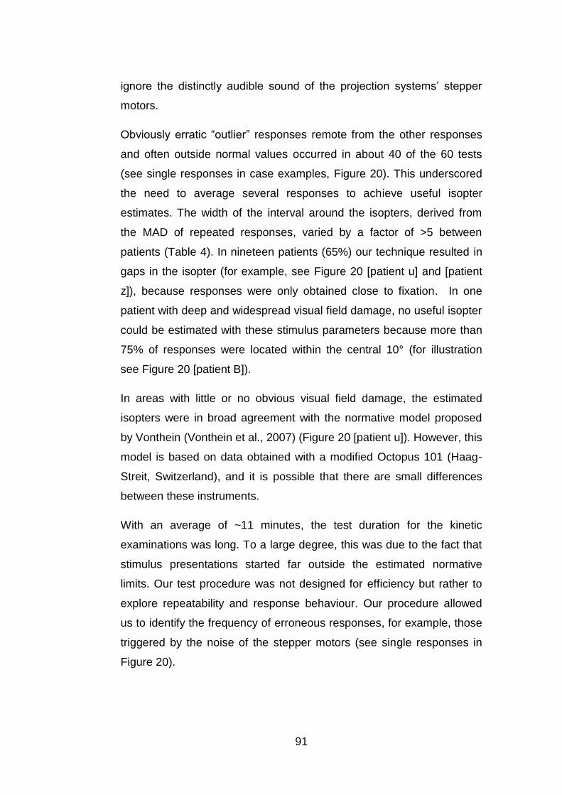
91
ignore the distinctly audible sound of the projection systems’ stepper
motors.
Obviously erratic “outlier” responses remote from the other responses
and often outside normal values occurred in about 40 of the 60 tests
(see single responses in case examples, Figure 20). This underscored
the need to average several responses to achieve useful isopter
estimates. The width of the interval around the isopters, derived from
the MAD of repeated responses, varied by a factor of >5 between
patients (Table 4). In nineteen patients (65%) our technique resulted in
gaps in the isopter (for example, see Figure 20 [patient u] and [patient
z]), because responses were only obtained close to fixation. In one
patient with deep and widespread visual field damage, no useful isopter
could be estimated with these stimulus parameters because more than
75% of responses were located within the central 10° (for illustration
see Figure 20 [patient B]).
In areas with little or no obvious visual field damage, the estimated
isopters were in broad agreement with the normative model proposed
by Vonthein (Vonthein et al., 2007) (Figure 20 [patient u]). However, this
model is based on data obtained with a modified Octopus 101 (Haag-
Streit, Switzerland), and it is possible that there are small differences
between these instruments.
With an average of ~11 minutes, the test duration for the kinetic
examinations was long. To a large degree, this was due to the fact that
stimulus presentations started far outside the estimated normative
limits. Our test procedure was not designed for efficiency but rather to
explore repeatability and response behaviour. Our procedure allowed
us to identify the frequency of erroneous responses, for example, those
triggered by the noise of the stepper motors (see single responses in
Figure 20).
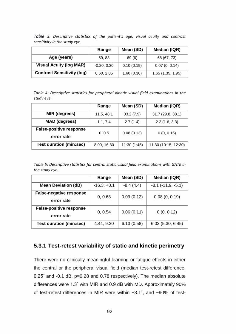
92
Table 3: Descriptive statistics of the patient’s age, visual acuity and contrast sensitivity in the study eye.
Range Mean (SD) Median (IQR)
Age (years) 59, 83 69 (6) 68 (67, 73)
Visual Acuity (log MAR) -0.20, 0.30 0.10 (0.19) 0.07 (0, 0.14)
Contrast Sensitivity (log) 0.60, 2.05 1.60 (0.30) 1.65 (1.35, 1.95)
Table 4: Descriptive statistics for peripheral kinetic visual field examinations in the study eye.
Range Mean (SD) Median (IQR)
MIR (degrees) 11.5, 48.1 33.2 (7.9) 31.7 (29.8, 38.1)
MAD (degrees) 1.1, 7.4 2.7 (1.4) 2.2 (1.6, 3.3)
False-positive response
error rate 0, 0.5 0.08 (0.13) 0 (0, 0.16)
Test duration (min:sec) 8:00, 16:30 11:30 (1:45) 11:30 (10:15, 12:30)
Table 5: Descriptive statistics for central static visual field examinations with GATE in the study eye.
Range Mean (SD) Median (IQR)
Mean Deviation (dB) -16.3, +0.1 -8.4 (4.4) -8.1 (-11.9, -5.1)
False-negative response
error rate 0, 0.63 0.09 (0.12) 0.08 (0, 0.19)
False-positive response
error rate 0, 0.54 0.06 (0.11) 0 (0, 0.12)
Test duration (min:sec) 4:44, 9:30 6:13 (0:58) 6:03 (5:30, 6:45)
5.3.1 Test-retest variability of static and kinetic perimetry
There were no clinically meaningful learning or fatigue effects in either
the central or the peripheral visual field (median test-retest difference,
0.25˚ and -0.1 dB, p=0.28 and 0.78 respectively). The median absolute
differences were 1.3˚ with MIR and 0.9 dB with MD. Approximately 90%
of test-retest differences in MIR were within ±3.1˚, and ~90% of test-

93
retest differences in MD were within ±2.10 dB (Figure 16 and Figure
17).
Figure 16: Test-retest variability of kinetic automated perimetry. Relationship between test-retest differences in mean isopter radius (MIR) and the range of peripheral visual field damage (mean of MIRs of 2 repeated tests). The height and width of the grey rectangle indicate the MAD scaled to a 90% range [-2.8˚, 3.3˚] and the range of mean MIRs [11.8˚, 48.1˚], respectively.
Figure 17: Test-retest variability of static automated perimetry. Relationship between test-retest differences in mean deviation (MD) and the range of central visual field damage (mean of MDs of 2 repeated tests). The height and width of the grey rectangle indicates the MAD scaled to a 90% range: [-2.2dB, 2.0dB] and the range of mean MDs [-16.3dB, 0.1dB], respectively.

94
A quantitative comparison of retest variability between SAP and KAP is
problematic – after all, different regions of the visual field are measured
with different estimation techniques and with different units of
measurement. I therefore related the spread of the retest differences to
the range of measures obtained in this sample (Figure 16 for peripheral
kinetic visual field tests, Figure 17 for central static visual field tests).
The range of the best estimate summary measures in this sample
(Figure 16 and Figure 17, width of the grey rectangle) to the spread of
test-retest differences (height of the rectangle) was similar for central
and peripheral examinations. Thus, the repeatability of KAP in the
peripheral field appears to be at least equivalent if not better than that of
SAP in the central visual field.
5.3.2 Relationship between peripheral and central visual
fields.
Our results confirmed the lack of a close relationship between
peripheral and central visual fields. The Spearman rank order
correlation between MIR and MD was rho = 0.51 (95% CI: [0.18, 0.74]).
This correlation is considerably lower than the correlations between test
and retest MD (rho = 0.89, 95% CI: [0.78, 0.95]) and MIR (rho = 0.92,
95% CI: [0.84, 0.96]). This suggests that the loose relationship between
central and peripheral visual field estimates in the data is not caused by
poor repeatability of the tests.
Some patients with deep central losses showed a nearly normal
peripheral isopter (Figure 20 [patient z]) while others with similar or less
severe central damage showed a severely constricted isopter (Figure
20 [patient e]). Similarly, in patients with severe central visual field
damage, the extent of the peripheral isopters varied substantially (for an
example see Figure 20 [patient B] and [patient f]).
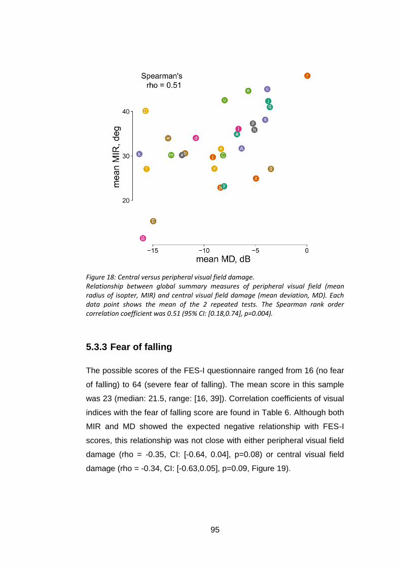
95
Figure 18: Central versus peripheral visual field damage. Relationship between global summary measures of peripheral visual field (mean radius of isopter, MIR) and central visual field damage (mean deviation, MD). Each data point shows the mean of the 2 repeated tests. The Spearman rank order correlation coefficient was 0.51 (95% CI: [0.18,0.74], p=0.004).
5.3.3 Fear of falling
The possible scores of the FES-I questionnaire ranged from 16 (no fear
of falling) to 64 (severe fear of falling). The mean score in this sample
was 23 (median: 21.5, range: [16, 39]). Correlation coefficients of visual
indices with the fear of falling score are found in Table 6. Although both
MIR and MD showed the expected negative relationship with FES-I
scores, this relationship was not close with either peripheral visual field
damage (rho = -0.35, CI: [-0.64, 0.04], p=0.08) or central visual field
damage (rho = -0.34, CI: [-0.63,0.05], p=0.09, Figure 19).
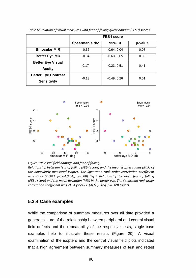
96
Table 6: Relation of visual measures with fear of falling questionnaire (FES-I) scores
FES-I score
Spearman’s rho 95% CI p-value
Binocular MIR -0.35 -0.64, 0.04 0.08
Better Eye MD -0.34 -0.63, 0.05 0.09
Better Eye Visual
Acuity 0.17 -0.23, 0.51 0.41
Better Eye Contrast
Sensitivity -0.13 -0.49, 0.26 0.51
Figure 19: Visual field damage and fear of falling. Relationship between fear of falling (FES-I score) and the mean isopter radius (MIR) of the binocularly measured isopter. The Spearman rank order correlation coefficient was -0.35 (95%CI: [-0.64,0.04], p=0.08) (left). Relationship between fear of falling (FES-I score) and the mean deviation (MD) in the better eye. The Spearman rank order correlation coefficient was -0.34 (95% CI: [-0.63,0.05], p=0.09) (right).
5.3.4 Case examples
While the comparison of summary measures over all data provided a
general picture of the relationship between peripheral and central visual
field defects and the repeatability of the respective tests, single case
examples help to illustrate these results (Figure 20). A visual
examination of the isopters and the central visual field plots indicated
that a high agreement between summary measures of test and retest

97
was reflected in similar shapes and patterns of the visual field plots
between test and retest (see Figure 20 [patient u, e, z and f]). Patient C
illustrates an example of a patient with high test-retest variability in both
the central and peripheral visual field. The high retest variability was
also reflected in a higher scatter of responses during each kinetic test of
patient C (MAD: test 1: 5˚, test 2: 4˚). The loose relation between the
extent of central and peripheral visual field damage also becomes
apparent in the visual field plots. Some patients showed a high
agreement between central and peripheral damage (see for example
Figure 20, patient u). Patient u’s central field showed a dense inferior
arcuate scotoma with a nasal step. The III1e isopter (dark green)
showed that the nasal step extended far into the periphery. Elsewhere
the isopter did not appear to be distinctly abnormal in comparison to
normative data. In other patients the relation was more ambiguous.
Patients e and z give an example of two patients with a similar degree
of central visual field loss, but very differently affected isopters. Patient
e had deep focal damage and some moderate diffuse damage in the
central superior visual field, but a substantially preserved peripheral
III1e isopter. Patient z had moderate diffuse central visual field damage,
but a substantially constricted III1e isopter (MIR: 25˚. In comparison, an
MIR around 47˚ would be expected in a healthy person of the same
age). Patient B shows an example of a patient with substantial central
and peripheral visual field loss. Only a central island of vision within the
central 5˚ appears to be preserved. A meaningful isopter could not be
estimated for patient B as most responses occurred close to fixation
within the central 10˚. The visual field plots for all participants of the
study are depicted in Appendix 1, from page 200 onwards.

98
Figure 20: Case examples of test and retest of the peripheral and central examination in one eye of six patients [patients u, e, z, f, B and C]. Both central and peripheral visual field examinations are depicted in one graphic by overlaying the greyscale representation of the GATE examination with a plot of the kinetic isopter. Eccentricities and test meridians are indicated by grey circles and dotted lines. Single responses to kinetic stimuli are shown as red dots. The measured isopter is plotted in dark green. Median responses < 10˚ were treated as “missing data” and appear as gaps in the isopter. The MAD measuring the scatter of single responses is shown as a green band surrounding the isopter, and normative values (Vonthein et al., 2007) are represented in light green.
99
5.4 Discussion
The objective of this study was to explore the relation between central
and peripheral visual field damage in glaucoma, and to investigate
retest variability of isopters that are estimated from repeated stimulus
presentations.
The results confirmed that patients with similar central visual field loss
may have rather different peripheral visual fields. The disparity in
central and peripheral visual field damage in patients with moderate to
severe glaucoma underscores that peripheral perimetry may be an
important step towards a more complete assessment of patients’ visual
field-related functional impairment. The results further suggest that a
simple approach of fully automated kinetic perimetry can reliably
estimate the extent of the peripheral visual field.
To avoid lens rim artefacts, refractive errors were not corrected for the
peripheral visual field test. However, both detection and resolution
acuity in the periphery are limited, not only through the lower cell
density in the peripheral retina, but also through optical defocus.
Detection acuity is more affected by defocus than resolution acuity,
which is mostly sampling-limited (Anderson, 1996). Non-corrected
refractive errors thus influence the detection rate and might lower
thresholds and introduce additional variability. Moreover, due to the
spherical nature of the lens, peripheral, off-axis stimuli cause
aberrations such as oblique astigmatism (Ferree et al., 1931a, Lotmar
and Lotmar, 1974, Millodot and Lamont, 1974). An off-axis circular
stimulus, for example, appears as an elliptic shape on the retina and not
as a circle and covers a wider space than the same stimulus in a central
region of the visual field. It should be noted that such aberrations
introduce differences between the same stimuli in the central versus
peripheral visual field and might influence their detection.
100
One of the pitfalls in automating kinetic perimetry is that isopter
locations based on single responses are highly error-prone. Lynn et al.
described the resulting phenomenon as “spurious spikes” in isopters
(Lynn et al., 1990). As in Lynn’s data, the results of this study revealed
obvious spurious responses in most of the automated kinetic exams.
One solution to reducing the impact of errors is to sample more
responses. Nowomiejska et al., for example, measured along 24
instead of the traditionally recommended 12 meridians (Nowomiejska et
al., 2005). In contrast, I increased the sampling by repeating
presentations; this approach also provides information about the
precision of the isopter estimates at each location.
Previous studies estimated repeatability of kinetic perimetry either
qualitatively, by comparing the classification of visual field results
according to defect types and locations, or quantitatively by comparing
visual field measures in test and retest (Quinn et al., 1991, Gramer et
al., 1980, Bittner et al., 2011, Ross et al., 1984a, Pineles et al., 2006,
Nowomiejska et al., 2005, Ramirez et al., 2008, Rowe and Rowlands,
2014, Hirasawa and Shoji, 2014, Bjerre et al., 2014). Reproducibility of
global estimates from SKP has previously been reported (Nevalainen et
al., 2008, Ramirez et al., 2008, Bjerre et al., 2014). MIR retest
differences of ±3.0˚ for III1e stimuli suggest that our approach of KAP
provides global estimates with at least equivalent precision. The
repeatability of this data also compare very favourably to those obtained
by Hirasawa et al. (Hirasawa and Shoji, 2014).
In this study the emphasis of the technique was not on efficiency, but
rather investigating repeatability and response behaviour in kinetic
perimetry. Large gains in efficiency may be achieved through an
adaptive technique which presents further stimuli according to the
already obtained responses. For example, a third presentation may not
be required when the previous two responses were close together. This
question is further explored in Chapter 6. This would allow for feasible

101
test durations without compromising reliability as in automated
approaches with only one stimulus presentation per meridian. Such
approaches are best designed with the help of simulations in which
responses similar to those of real patients are generated. In this way, a
large number of different scenarios with various test strategies and
visual field defects can be systematically explored in a short time. The
individual response data obtained as a by-product of this research will
contribute to the empirical data necessary for such work. Ultimately,
simulations will also be helpful for deciding in which situations kinetic
stimuli are more efficient than static stimuli for estimating the peripheral
visual field.
Also, it may be not be necessary to examine the entire circumference of
the isopter. Instead, a test could focus on those areas that are most
informative functionally (Black et al., 2011) or clinically (LeBlanc and
Becker, 1971). For a wider dynamic range stimulus parameters might
have to be adjusted in patients with end-stage glaucomatous visual field
defects (see Figure 20 [patient B]) (Nowomiejska et al., 2014, Tonagel
et al., 2012, Scheuerle et al., 2012). An exploratory scan prior to the
examination as suggested by Johnson et al. might be beneficial to
choose suitable stimulus parameters (Johnson et al., 1987).
Adaptive kinetic tests, perhaps in conjunction with static perimetry of the
central visual field (Johnson et al., 1987, Pineles et al., 2006, Miller et
al., 1989), might provide a fruitful avenue for further development of
perimetry for patients with moderate and advanced visual field damage.
While the current study was not designed to answer the question of
whether and by how much the visual field periphery contributes to real-
world visual problems (Haymes et al., 2007, Black et al., 2011, Glen et
al., 2014, Glen et al., 2011, Szlyk et al., 2005), such research will be
important to conduct in the future. Considering the many risk factors for
falls (Rubenstein and Josephson, 2002, Dhital et al., 2010, Moenter et
al., 2014), the lack of a close relationship between the visual field

102
indices and the fear-of-falling questionnaire scores (correlation
coefficients around -0.35) is not surprising. However, these
relationships appeared at least as strong if not stronger than those seen
with visual acuity (R=0.17) and contrast sensitivity (R=-0.13). Based on
the correlation coefficients estimated in this study, I estimate that
sample sizes of at least 100 patients would be required to investigate
the relation between visual field indices and fear of falling with sufficient
power, and substantially larger samples (around 300 patients) would be
required to distinguish between central and peripheral visual field
predictors.

103
6. Simulating response behaviour to
kinetic stimuli
6.1 Introduction
In the clinical environment short test durations are essential. A strategy
for automated kinetic perimetry in the peripheral visual field should be
efficient, i.e. it should achieve good accuracy and precision with a
minimal number of presentations. This chapter investigates the
relationship between the number of presented stimuli per meridian and
the accuracy and precision of the estimation of isopter locations with
repeated presentations through a simulation of responses to kinetic
stimuli.
A key advantage of simulations over experiments with human observers
is that the true underlying sensitivity is known, and therefore, the error
(difference between the estimate and the true value) can be
determined. Moreover, simulations make it possible to evaluate the
performance of many different test strategies in a short amount of time.
They have been extensively used to evaluate threshold estimation
procedures in static automated perimetry to estimate accuracy
(Spenceley and Henson, 1996) or compare the efficiency of different
test procedures (Turpin et al., 2003). Many of the simulations rely on
Henson et al.’s model of the relation between response variability and
contrast sensitivity (see Chapter 7) (Gardiner and Crabb, 2002a,
Gardiner and Crabb, 2002b, Turpin et al., 2003, Turpin et al., 2007,
Henson et al., 2000).
However, to my best knowledge, there is little literature on simulations
of kinetic perimetry (Schiefer et al., 2006a, Shapiro et al., 1988, Shapiro
and Johnson, 1990). Shapiro et al. developed a computer simulation

104
procedure for various types of perimetry including kinetic and static
perimetry called KRAKEN (Shapiro et al., 1988). The model for
simulating kinetic perimetry was based on data from manual Goldmann
examinations. The isopter locations estimated with Goldmann perimetry
were converted into contrast sensitivity values based on the size and
intensity of the respective Goldmann stimulus. They then introduced
variability to the contrast sensitivity in the form of a Gaussian that, as
chosen, could depend on eccentricity, age and area of visual field loss.
Additional noise in the form of false positive and false negative rates
could also be added.
However, it is unclear what the actual distribution of kinetic responses
around the isopter location looks like. In particular, a Gaussian
distribution might be unsuitable. In this chapter I will estimate the
distribution of responses to kinetic stimuli around isopter locations
based on the data from Chapter 5.
Due to the nature of kinetic perimetry (stimuli being moved from areas
with lower expected sensitivity to areas with higher expected sensitivity
of the visual field), response variability manifests in distances of
responses from the location of detection. Intrinsic variability in the
retinal location at which the signal becomes strong enough to elicit a
conscious percept of the stimulus is probably one part of that variability.
But other factors likely lead to much larger variations in the responses.
Fatigue or low attention could for example affect response times and
lead to increased false positive and false negative rates. False positive
responses can even occur at long distances from the true location of
detection. Notably, in kinetic perimetry, false negative responses cannot
simply be defined as the absence of a response to a stimulus
presentation, but rather the absence of the response at the time of first
detection of the stimulus. Since stimuli move across the visual field until
they are either detected or reach an endpoint (often at fixation), a
response is likely to still occur after a false negative at a later point of

105
the stimulus presentation. Thus even false negative responses
indirectly add to the variability of the distribution of response around the
location of detection.
To simulate response behaviour to kinetic stimuli in the entire visual
field, a model needs to be established that relates the parameters of the
stimuli (size, contrast, speed) to respective probability distributions of
responses around the isopter. In this chapter, only one stimulus type is
taken into account (Goldmann III1e), and simulations of kinetic
responses are based on the distribution of responses to Goldmann III1e
stimuli that were moved at a speed of 5˚/sec.
However, even when using the same stimulus parameters, several
factors might still affect response variability. There could be a
sequential dependency of response variability (caused by e.g. learning
effects or fatigue). The variability of responses might also differ
depending on the location in the visual field. It could change with visual
field eccentricity or differ for example between the nasal and temporal
visual field. Should these factors be closely related to response
variability they have to be included in a model to simulate responses to
kinetic stimuli.
Thus, in this chapter I (1) examine the dependency of response
variability on various factors (order of presentation, eccentricity,
meridian) (2) investigate the probability distribution of responses to
kinetic stimuli around the estimated isopter and (3) simulate kinetic
responses based on the probability distribution of responses to evaluate
how many responses are required to achieve good accuracy and
precision of isopter estimates.
The aim of this chapter is to demonstrate the usefulness of simulations
to develop efficient strategies for kinetic automated perimetry.
106
6.2 Methods
6.2.1 Kinetic visual field test:
The kinetic response data used in this study was the same as described
in Chapter 5. Thirty patients with glaucoma performed two automated
kinetic perimetry tests in one eye on the same day. Single peripheral
isopters were measured in each of the two tests along 16 meridians
with three Goldmann III1e stimuli presented per meridian at a speed of
5˚/sec (see Chapter 5.2.2.1.1, page 87, for further details on the
procedure). For the purpose of evaluating patients’ response behaviour
the response data from test and retest was pooled together resulting in
six stimulus presentations per meridian per person, thus giving a total of
96 presentations per person.
6.2.2 Analyses
The isopter location on each meridian was estimated as the median of
six responses, i.e. the mean of the two middle responses. The kinetic
response data was used to estimate the distribution of single responses
around the estimated isopter location. Since the proposed application of
automated kinetic perimetry is measuring the peripheral visual field, all
responses that resulted in isopter locations within the central 10˚ were
removed from the data set prior to any further analysis.
The difference of each response from the respective estimated isopter
location is referred to as scatter of responses. The response variability
for each isopter location of each patient was estimated by the median
absolute deviation (MAD) of responses from the estimated isopter
location at the respective meridian. To investigate whether response
behaviour changed with the time course of a test (related to fatigue or a
learning effect) or depending on the location in the visual field, we
tested for sequential dependencies of the scatter of responses and

107
examined the relation of response variability with eccentricity and
meridian position in the visual field, respectively.
Data analysis was performed in R (version 2.15.1, (R-Core-Team,
2012)) and Matlab (MathWorks, 2008). To estimate the sequential
dependency of scatter, the distances of each response from the isopter
location were correlated with the ordinal numbers reflecting the
sequence of the presentations of stimuli using a Spearman correlation.
The relation between the eccentricity of isopter locations in the visual
field and response variability was explored by correlating the
eccentricity of the estimated isopter locations with the median absolute
deviation of the responses around the respective isopter location.
Finally, a circular linear correlation between the median absolute
deviations and circular position in the visual field defined by the
meridian was performed.
The circular linear correlation was calculated with the CircStat Matlab
toolbox (Berens, 2009). There an association between a directional
variable α and a linear variable x is estimated by correlating x with cos α
and sin α individually. The individual Pearson correlation coefficients rsx
= c(sin α, x), rcx = c(cos α, x) and rcs = c(sin α, cos α) are correlated first.
Finally, the circular linear correlation ρcl is defined as:
Equation 6: Circular linear correlation ((Zar, 1999), Equation 27.47 cited in Berens 2009)
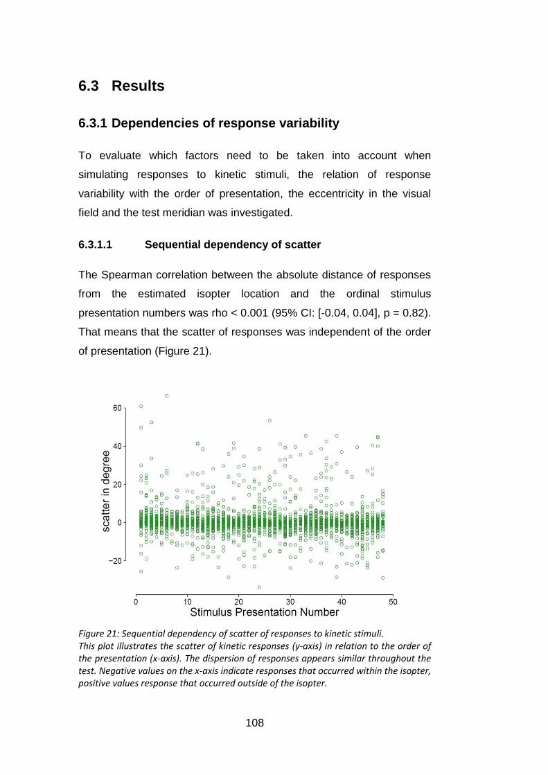
108
6.3 Results
6.3.1 Dependencies of response variability
To evaluate which factors need to be taken into account when
simulating responses to kinetic stimuli, the relation of response
variability with the order of presentation, the eccentricity in the visual
field and the test meridian was investigated.
6.3.1.1 Sequential dependency of scatter
The Spearman correlation between the absolute distance of responses
from the estimated isopter location and the ordinal stimulus
presentation numbers was rho < 0.001 (95% CI: [-0.04, 0.04], p = 0.82).
That means that the scatter of responses was independent of the order
of presentation (Figure 21).
Figure 21: Sequential dependency of scatter of responses to kinetic stimuli. This plot illustrates the scatter of kinetic responses (y-axis) in relation to the order of the presentation (x-axis). The dispersion of responses appears similar throughout the test. Negative values on the x-axis indicate responses that occurred within the isopter, positive values response that occurred outside of the isopter.
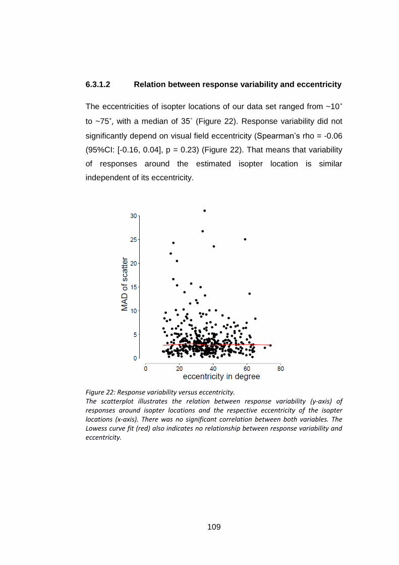
109
6.3.1.2 Relation between response variability and eccentricity
The eccentricities of isopter locations of our data set ranged from ~10˚
to ~75˚, with a median of 35˚ (Figure 22). Response variability did not
significantly depend on visual field eccentricity (Spearman’s rho = -0.06
(95%CI: [-0.16, 0.04], p = 0.23) (Figure 22). That means that variability
of responses around the estimated isopter location is similar
independent of its eccentricity.
Figure 22: Response variability versus eccentricity. The scatterplot illustrates the relation between response variability (y-axis) of responses around isopter locations and the respective eccentricity of the isopter locations (x-axis). There was no significant correlation between both variables. The Lowess curve fit (red) also indicates no relationship between response variability and eccentricity.
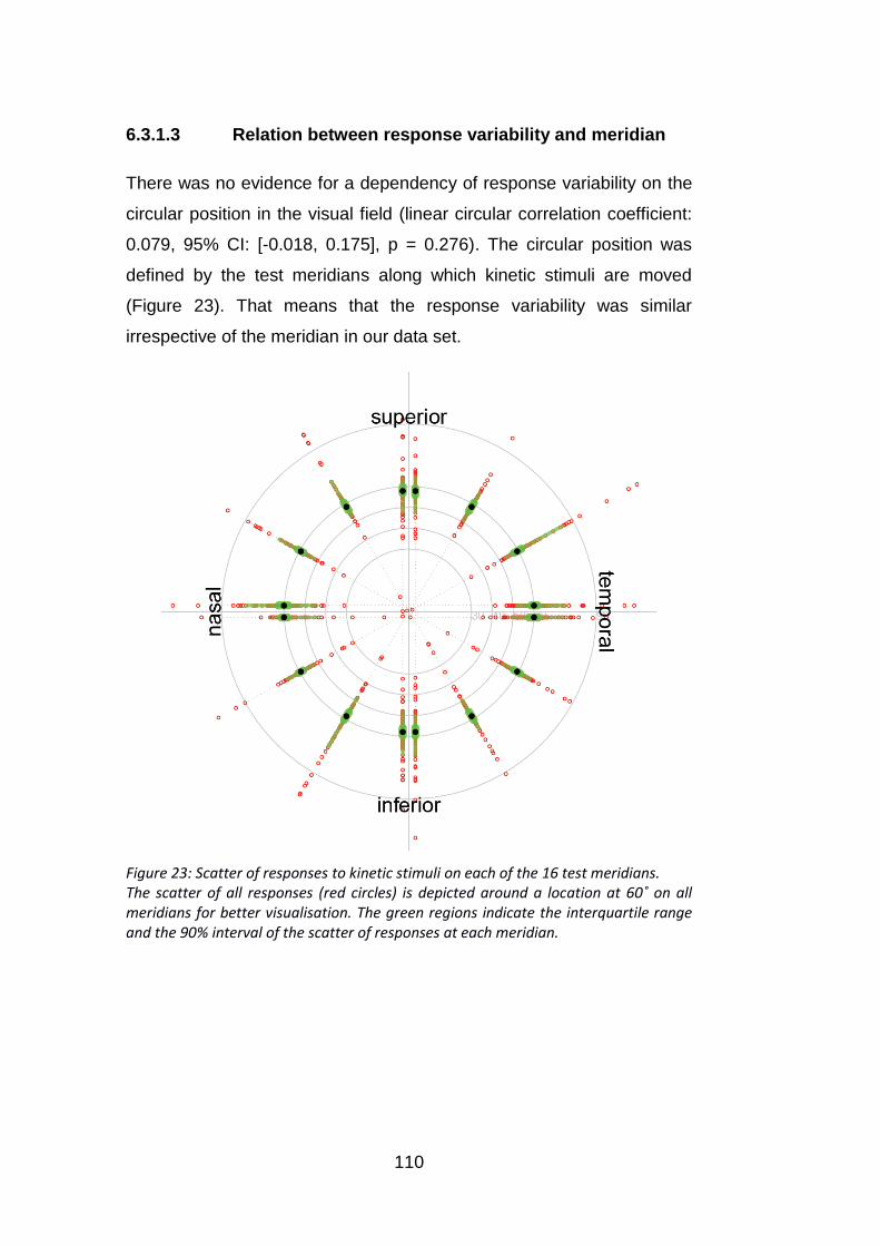
110
6.3.1.3 Relation between response variability and meridian
There was no evidence for a dependency of response variability on the
circular position in the visual field (linear circular correlation coefficient:
0.079, 95% CI: [-0.018, 0.175], p = 0.276). The circular position was
defined by the test meridians along which kinetic stimuli are moved
(Figure 23). That means that the response variability was similar
irrespective of the meridian in our data set.
Figure 23: Scatter of responses to kinetic stimuli on each of the 16 test meridians. The scatter of all responses (red circles) is depicted around a location at 60˚ on all meridians for better visualisation. The green regions indicate the interquartile range and the 90% interval of the scatter of responses at each meridian.

111
6.3.2 Estimation of the distribution of responses around
the isopter location
Since the data revealed no significant dependencies between response
variability and eccentricity, meridian or the order of stimulus
presentation, the distribution of the responses around isopter locations
was estimated independent of these factors.
The response variability of each patient was estimated via the median
absolute deviation of all responses around the estimated isopter
locations. Figure 24 (left) shows the probability density function of
response variability of all patients fitted with a Gaussian kernel with a
smoothing bandwidth (standard deviation) of 1.6.
Figure 24: Distribution of response variability over all patients. Left: Distribution of median absolute deviations of scatter for the 30 patients fitted with a Gaussian kernel with a bandwidth of 1.6. Right: The q-q plot compares the distribution of the response variability to a normal distribution. Data points deviating from the grey line indicate a non-normal distribution. The distribution has a tail to the right, which indicates that response variability substantially higher than average occasionally occurs.
The median absolute deviations of responses from isopter locations in
this data set ranged from 1˚ to 9˚ between patients with a median of 3˚.
Thus the overall scatter of responses around the isopter locations
ranged widely between participants (Figure 25, left). To estimate the

112
distribution of the scatter of the responses around the isopter locations,
it was first normalised by the response variability (MAD) of each patient.
Figure 25 shows the scatter of responses for each person before (left)
and after (right) normalisation by individual response variability.
Figure 25: Scatter of responses around the estimated isopter location for each participant. Letter identifiers for participants match the identifiers used in Chapter 5. Left: The distance of each response from the estimated isopter location is shown for each patient. Negative values represent responses within the estimated isopter, positive values those outside the estimated isopter. Right: the scatter of responses is normalised by the median absolute deviation of respective participants.
Following the normalisation the data were pooled together and the
overall distribution of responses around isopter locations was estimated
and fitted with a Gaussian kernel (Figure 26, left). The q-q plot (right)
emphasizes that the distribution is non-normal and positively skewed
with long tails. The slightly longer left tail indicates that responses occur
in larger distances outside of the isopter location than within. This could
be caused by a higher likelihood of early (false positive) than late
responses.

113
Figure 26: Distribution of normalised scatter of responses for all patients. Left: Distribution of normalised scatter of responses around isopter locations. Negative values on the x-axis indicate responses occurring within the estimated isopter and positive values indicate responses outside of the estimated isopter. The distribution is non-normal and has long tails and indicates that a vast majority of responses are closely spaced to isopter locations while occasional responses occur at larger distances from the isopter. The best fitting normal distribution is depicted in grey. Right: The q-q plot compares the distribution of the scatter of responses around the isopter to a normal distribution. Data points deviating from the grey line indicate a non-normal distribution. The distribution has long tails in both directions and is slightly skewed towards the right, which indicates that responses occur at larger distances outside than within the isopter.
6.3.3 Simulating kinetic responses
6.3.3.1 Simulating isopters based on kinetic response
behaviour
Since the data revealed no dependencies of response variability with
the order of stimulus presentation or the location in the visual field, the
same distribution of responses around the true isopter location is
assumed independent of eccentricity, meridian or test sequence.
Response variability differed strongly between patients. The simulation
of kinetic responses was based on two aspects: the distribution of
response variability present in different patients (Figure 24, left) and the
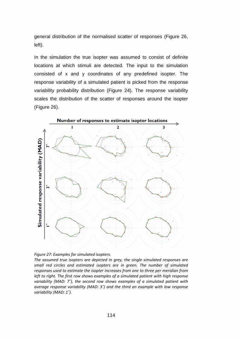
114
general distribution of the normalised scatter of responses (Figure 26,
left).
In the simulation the true isopter was assumed to consist of definite
locations at which stimuli are detected. The input to the simulation
consisted of x and y coordinates of any predefined isopter. The
response variability of a simulated patient is picked from the response
variability probability distribution (Figure 24). The response variability
scales the distribution of the scatter of responses around the isopter
(Figure 26).
Figure 27: Examples for simulated isopters. The assumed true isopters are depicted in grey, the single simulated responses are small red circles and estimated isopters are in green. The number of simulated responses used to estimate the isopter increases from one to three per meridian from left to right. The first row shows examples of a simulated patient with high response variability (MAD: 7˚), the second row shows examples of a simulated patient with average response variability (MAD: 3˚) and the third an example with low response variability (MAD: 1˚).
115
Consequently, a simulated patient with larger response variability has a
wider range of scatter of responses around the true isopter location
(Figure 27). The distance of responses from isopter locations is
determined by drawing from the scatter distribution scaled with the
chosen response variability. The scatter is added to the true isopter
location to determine the location of single simulated responses.
6.3.3.2 Accuracy and precision of isopter estimation with
increasing number of measures per meridian
Here, I used the simulation of kinetic responses to investigate how the
accuracy and precision of the estimation of isopter locations depends
on the number of stimuli used to estimate said isopter.
Isopters were simulated with increasing numbers of stimulus
presentations per meridian ranging from one stimulus to twenty. For
each number of stimuli, isopters were simulated 1000 times, with 16
isopter locations per iteration and responses were drawn according to
probability density functions of response variability (Figure 24) and
scatter (Figure 26). The absolute distance between estimated and true
isopter locations (error) was on average 5˚ (mean) with one response,
3.9˚ with two responses and 2.1˚ with three responses (Figure 28, right).
The interquartile ranges and 90% intervals illustrate a low precision of
the isopter estimation with one or two responses (Figure 28, left).
Adding a third stimulus decreases the 90% interval of the error by more
than half (Figure 28), which demonstrates a large gain in precision.
Adding further stimuli led to relatively small gains in precision. The
mean error showed that, on average, there is a bias towards estimating
the true isopter to be located further outside the isopter (mean error:
1.2˚) when using only one or two stimuli. This bias is reduced when
adding a third stimulus and is then close to zero (0.2˚) (Figure 28, left).

116
Figure 28: Precision of isopter location estimation with increasing number of measures per meridian. The deviation between estimated and true isopter locations (error) is displayed on the y-axis and the number of presentations per meridian on the x-axis. Left: Error versus number of questions: negative values of the error indicate estimated isopter locations within the isopter and positive values those outside. Right: Absolute error versus number of questions. Isopters were estimated 1000 times for each condition. Green dots indicate the median, green lines the interquartile range and errorbars give the 90% interval of the distances between true and estimated isopter locations over 16 locations and 1000 iterations. Small red dots indicate the mean error.
The relation between the number of stimuli to estimate isopter locations
and the accuracy of the locations indicates that at least three responses
are necessary to get accurate isopter estimates in most patients.
However, additional rules could be implemented into kinetic procedures.
For example a third stimulus could only be presented if the distance
between the first two responses exceeds a critical range. The accuracy
and precision of isopter locations estimated with two responses was
found to be similar to that of isopter locations estimated with three
responses, when the two stimuli were maximally spaced 10˚ apart from
each other (Figure 29). According to results of the simulation, two
responses to a kinetic stimulus occur in a distance of less than 10˚ from
each other in 80% of the cases. Thus a third stimulus would only be
required in 20% of the cases.
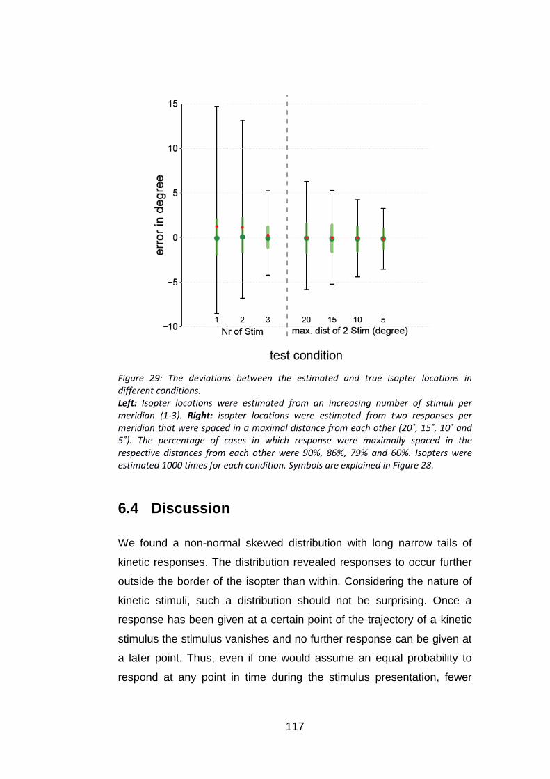
117
Figure 29: The deviations between the estimated and true isopter locations in different conditions. Left: Isopter locations were estimated from an increasing number of stimuli per meridian (1-3). Right: isopter locations were estimated from two responses per meridian that were spaced in a maximal distance from each other (20˚, 15˚, 10˚ and 5˚). The percentage of cases in which response were maximally spaced in the respective distances from each other were 90%, 86%, 79% and 60%. Isopters were estimated 1000 times for each condition. Symbols are explained in Figure 28.
6.4 Discussion
We found a non-normal skewed distribution with long narrow tails of
kinetic responses. The distribution revealed responses to occur further
outside the border of the isopter than within. Considering the nature of
kinetic stimuli, such a distribution should not be surprising. Once a
response has been given at a certain point of the trajectory of a kinetic
stimulus the stimulus vanishes and no further response can be given at
a later point. Thus, even if one would assume an equal probability to
respond at any point in time during the stimulus presentation, fewer
118
responses would be expected at a later point time. For example, if the
probability to respond at a certain location would be 25% (one fourth),
this would influence the next location, since the stimulus will not be
presented there if an answer already occurred. Thus the stimulus would
only reach the next location three out of four times. The probability for a
response in that location would thus be three fourth times one fourth
and would lie at only 18.75%. While this principle will govern the
distribution of responses to some extent the response behaviour is
certainly more complex. The probability to give a response once a
stimulus can be detected is certainly higher than to give a false positive
response. Furthermore the eagerness to press the button might
increase the longer a person waits for a stimulus to appear (change in
response criterion).
The scatter of responses did not depend on the order of stimulus
presentation. Thus there was no apparent fatigue or learning effect.
The response variability in our data set did not vary with the location in
the visual field, be it eccentricity or orientation of the meridian. Since the
same stimulus type (Goldmann III1e) was used, the locations of
detection should have similar contrast sensitivities independent of
eccentricity. Thus, the lack of a relationship between response
variability and eccentricity might be related to a constant relation
between contrast sensitivity and response variability. Such a constant
relation between response variability and contrast sensitivity has been
demonstrated for static stimuli (Henson et al., 2000).
A previous study found response variability to kinetic stimuli to increase
with visual field eccentricity in participants with normal vision (Parrish et
al., 1984). Parrish et al. related this increase in response variability to a
flattening of the hill of vision in the peripheral visual field. The similar
response variability independent of eccentricity in patients with
glaucoma might be related to a local flattening of the hill of vision in
areas of visual field loss. Notably, the measures of response variability
119
differ in this and Parrish et al.’s study (median absolute deviation versus
standard deviation).
The simulations showed that repeated presentations are required to
estimate isopter locations with good accuracy and precision. The
largest gain in both accuracy and precision in the estimation of isopter
locations is achieved when increasing the number of responses used to
estimate isopter locations up to three. Thus a minimum of three
responses should be used to get accurate isopter estimates. However,
the test duration of a kinetic visual field examination with three
repetitions per isopter location might still be too long for the clinical
environment. The use of adaptive kinetic procedures would therefore be
promising. For example, a third stimulus could only be presented if the
distance between the first two responses exceeds a certain criterion.
According to the simulation, a similar accuracy and precision to the
three repeated presentations technique could be reached with such a
rule. A third stimulus presentation would then only be required in an
estimated 20% of the cases. That means, in a test strategy
implementing such a rule, only about 75% of the stimulus presentations
of a test with three repeated presentations are required to reach similar
precision.
It is clear that large gains in efficiency could be achieved through
adaptive techniques which presents further stimuli depending on the
already obtained responses or based on prior knowledge about the
visual field. This could result in short test durations without
compromising reliability. Simulations based on response data to kinetic
stimuli, as performed in this study, could be a helpful tool to explore
different strategies for kinetic perimetry. In this way, a large number of
different scenarios with various test strategies and visual field defects
could be systematically explored in a short time.
Certain limitations of the simulation of kinetic responses in this study
should be taken into consideration. In a true experiment the response

120
distribution would always be limited by the start and stop location of the
trajectory of the kinetic stimulus and by the respective distance of the
true isopter location from the start and stop location. A long distance
between the start location and the isopter location would for example
lead to an increased probability for responses outside of the isopter
border, as the time during which these responses can occur increases.
On the other end a small distance to the stop location would decrease
the opportunity for responses within the true isopter. These factors were
not taken into account in this model. Moreover, the probability
distribution of response variability based on the 30 participants was
smoothed to prevent an inordinate influence of single data points on the
probability distribution. This led to an inclusion of response variability
close to zero in the distribution. Notably, while these occurred at a very
low probability, it is unlikely that such response variability would ever be
present in actual patients.
Furthermore, I only examined kinetic responses to one Goldmann
stimulus type (III1e). Response variability might differ depending on the
overall stimulus intensity (size and contrast). To simulate response
behaviour to other Goldmann stimuli, response data to a wide range of
stimuli would be required.

121
7. Frequency-of-Seeing for static
perimetry on estimated isopter
locations in the peripheral visual
field
7.1 Introduction
Simulations can be a useful tool to determine efficient strategies for
measuring the peripheral visual field (see Chapter 6). In previous
studies simulations have been used to determine the efficiency of static
perimetric strategies in the central visual field (Spenceley and Henson,
1996, Turpin et al., 2003, Turpin et al., 2007, Gardiner and Crabb,
2002a, Gardiner and Crabb, 2002b). However, for the peripheral visual
field little data is available to base such simulations on. For automated
kinetic perimetry this is the case, since no standard automated kinetic
perimetry technique has been established yet. For static automated
perimetry, this is the case since the most commonly used static tests
concentrate on the central visual field.
As of yet, it is unclear, whether static or kinetic automated perimetry is
more suitable in the peripheral visual field.
This chapter looks into the estimation of contrast sensitivity in the
peripheral visual field with static stimuli. (1) I explore how the larger
Goldmann V stimulus affects contrast sensitivity and response
variability throughout the visual field in comparison to the Goldmann III
stimulus, which is typically used in SAP. (2) I investigate the relationship
between contrast sensitivity and response variability in the peripheral
compared to the central visual field and (3) I examine the relationship
between kinetic and static peripheral visual field measures.
122
7.1.1 Stimulus size in static perimetry
It has been previously suggested that stimuli with a larger area are
more suitable for visual field examinations in glaucoma as they are
picked up with higher sensitivity and lower response variability (Wall et
al., 2010, Wall et al., 2009, Wall et al., 1997, Gardiner et al., 2013).
Standard automated perimetry with Goldmann V stimuli has been found
to have a higher dynamic range than size III SAP by about 1 log unit
(Wall et al., 2010).
In this chapter we compare contrast sensitivity and response variability
to size III (0.43˚ diameter) and size V (1.72˚ diameter) stimuli in patients
with glaucoma and participants with normal vision throughout the visual
field. The gain in contrast sensitivity has been estimated to lie at 5 dB
for each increase in Goldmann stimulus size (4-fold increase in area)
(see Chapter 2.1.4.2, page 43-47) (Goldmann, 1999, Goldmann, 1945).
Thus the change in sensitivity from a size III to size V stimulus is
expected to lie at 10 dB on average. However, the difference in contrast
sensitivity to different stimulus sizes has been shown to increase with
eccentricity (Wilson, 1970, Dannheim and Drance, 1971, Wald, 1938).
The relationship between contrast sensitivity and stimulus size has
been connected to the summation of ganglion cell responses (Wilson,
1970, Swanson et al., 2004, Fischer, 1973, Anderson, 2006).
Depending on the size of a stimulus, light covers a certain area of the
retina. A certain number of ganglion cells receive input from that retinal
area. The larger the stimulus is and thus the retinal area that is covered
by the stimulus, the more ganglion cells will respond to the stimulus.
The more ganglion cells respond, the stronger is the signal. Up to a
certain number of ganglion cells an increase in stimulus area leads to
an equivalent increase in contrast sensitivity. At a certain level an
increase of the area and thus an activation of additional ganglion cells
does not lead to a strong gain in the signal and the slope of the relation
between area and contrast sensitivity flattens. The area at which this

123
slope starts to flatten is called Ricco’s area. Since ganglion cell density
is high in the central visual field and decreases towards the periphery, a
larger number of ganglion cells will respond to the same stimulus when
it falls onto a central instead of a peripheral visual field area.
Consequently, a larger area is required to activate the same number of
ganglion cells in the peripheral visual field. Thus the size of Ricco’s area
increases with eccentricity. This relationship has been found repeatedly
in psychophysical studies (Wilson, 1970, Redmond et al., 2010). Wilson
et al. demonstrated that contrast sensitivity remains constant
throughout the visual field if the stimulus size is adjusted to Ricco’s area
(see Chapter 2.1.4.2.1, page 45, Figure 6). Ganglion cell density can
also decrease as a result of a disease, such as glaucoma. Ricco’s area
has been found to increase in patients with glaucoma (Fellman et al.,
1988, Redmond et al., 2010).
Since an increase in the stimulus area allows the stimulus to fall into the
receptive field of more ganglion cells, the signal-to-noise ratio improves
with stimulus area. This is also reflected in a lower response variability
to larger stimuli (Vislisel et al., 2011, Wall et al., 2013, Wall et al., 1997,
Gardiner et al., 2013). However, an increase in stimulus area only
substantially improves the signal-to-noise ratio until Ricco’s area is
reached after which spatial summation of the signal decreases.
Since Ricco’s area increases in glaucoma, we expect to find a gain in
contrast sensitivity when testing with a size V instead of size III stimulus
throughout the visual field in patients with glaucoma. For the same
reason we expect a reduction in response variability. In the normal
visual field the Goldmann size III (0.43˚ diameter) matches Ricco’s area
at about 40˚ eccentricity (see Chapter 2.1.4.2.1, page 45, Figure 6)
(Anderson, 2006, Wilson, 1970). That means complete spatial
summation beyond a size III stimulus only occurs beyond 40˚ of
eccentricity. Thus we expect to find a larger difference in contrast
sensitivity and response variability between size III and V stimuli in the

124
peripheral than in the central visual field in participants with normal
vision.
7.1.2 Response variability to static stimuli
Previous studies suggest that response variability increases with
decreasing sensitivity (Henson et al., 2000, Weber and Rau, 1992,
Olsson et al., 1993, Chauhan et al., 1993, Russell et al., 2012a). That
means that threshold estimates at locations with lower contrast
sensitivity are less reliable. The increase in response variability with
lower contrast sensitivity has been speculated to be connected to an
activation of fewer ganglion cells leading to a worse signal-to-noise ratio
(Vislisel et al., 2011, Wall et al., 2013, Wall et al., 1997, Gardiner et al.,
2013, Redmond et al., 2010). Since ganglion cell density and contrast
sensitivity decrease with visual field eccentricity this suggests that
response variability increases with eccentricity. Contrast sensitivities
estimated at peripheral locations have been found to have higher
response variability (Weber and Rau, 1992).
In this chapter I explored how response variability changes with contrast
sensitivity in the peripheral compared to the central visual field. I
furthermore examined whether this relation differs between patients
with glaucoma and participants with healthy vision. Henson et al. found
a linear relationship between contrast sensitivity and logarithmically
scaled response variability (Henson et al., 2000). This established
relationship often served as a model for simulating response variability
in static automated perimetry (Gardiner and Crabb, 2002a, Gardiner
and Crabb, 2002b, Turpin et al., 2007, Turpin et al., 2003). Henson et
al. found no difference in the relation between response variability and
contrast sensitivity between normal vision, glaucoma (POAG), optic
neuritis and ocular hypertension. This finding corroborated the theory
that response variability increases with decreasing ganglion cell density
125
irrespective of its cause, be it visual disease or visual field eccentricity
in the healthy visual field. However, Henson et al. only measured within
the central 30˚ of the visual field. Thus it is unclear whether the
relationship between contrast sensitivity and response variability
remains the same further in the periphery. If the relationship between
sensitivity and response variability is identical in centre and periphery,
the peripheral points (with their lower sensitivity) may provide a model
for damaged central locations in glaucoma. If the relationship between
sensitivity and response variability is different in the peripheral than in
the central visual field, it can indicate that a reduction in ganglion cell
density caused by disease affects response variability in a different way
from the normal physiological reduction of ganglion cell density in the
peripheral visual field.
7.1.3 Relation between static and kinetic measurements
Both static and kinetic perimetry provide a mapping between contrast
sensitivity and visual field locations. However, while in static perimetry a
series of stimuli are presented for a short amount of time (200 ms each)
at one location to estimate a detection threshold, in kinetic perimetry
stimuli are moved across the visual field, generally from the periphery
where they are “unseen” towards the centre until they are first detected.
Thus the properties of the measurements are very different. Static
perimetry provides a threshold estimate at a specific location. However,
the estimated threshold can vary from one examination to another.
Kinetic perimetry provides a location at which a certain stimulus
intensity can be detected. However, the measured location can vary
between examinations.
Even if the location at which a kinetic stimulus is detected could be
determined with absolute accuracy and precision, the sensitivity to a
static stimulus might still be different. A dissociation between contrast

126
sensitivity to kinetic and static stimuli (stato-kinetic dissociation) has
been described previously and was found to be present in normal
vision, as well as with pre- and post lateral geniculate nucleus lesions
(Schiller et al., 2004, Riddoch, 1917, Finkelstein and Johnson, 1989,
Safran and Glaser, 1980, Hudson and Wild, 1992, Schiller et al., 2006,
Casson et al., 1991). This dissociation is often referred to as the
Riddoch phenomenon (Riddoch, 1917, Safran and Glaser, 1980) or
statokinetic dissociation. Typically sensitivity appears to be greater to
moving than to static stimuli. In contrast, this appears to be reversed in
the macula, as sensitivity has been found to be higher to static stimuli at
2˚ eccentricity (Fankhauser and Schmidt, 1960). The cause for this
dissociation may be the activation of different visual pathways by
moving and kinetic stimuli, the longer presentation time of the kinetic
stimulus, the larger retinal area over which the kinetic stimulus is moved
until it is detected (spatial summation), or the possibility that observers
adopt different criteria in responding to static or kinetic stimuli. Given
the dissociation between static and kinetic stimuli it is hard to directly
compare visual field measures from static and kinetic procedures.
Therefore, to compare results from kinetic and static examinations, one
needs to know how to translate them into a common reference frame.
Here, I investigate the difference between sensitivity to kinetic III1e
stimuli and static size III stimuli. I also examine whether the difference
between the measures changes depending on visual field eccentricity
or test meridian.
7.1.4 Study design
In this study, I measured frequency-of-seeing to static Goldmann size III
stimuli at kinetically estimated III1e isopter locations. This design allows
a) to compare static and kinetic measurements and b) to estimate

127
sensitivity and response variability to static stimuli in peripheral
locations that are unlikely to fall into areas of deep losses (near 0 dB) in
patients with glaucoma.
Additional locations for the frequency-of-seeing test were chosen at
predefined locations in the central visual field to compare the relation
between sensitivity and response variability in the central and peripheral
visual field. Frequency-of-seeing was also measured with static
Goldmann V stimuli at all locations to investigate the influence of the
larger stimulus on contrast sensitivity and response variability in the
central and peripheral visual field.
The study was designed by VM Mönter and PH Artes. All tests were
designed to run on the Octopus 900 (Haag-Streit, Koeniz, Switzerland).
The kinetic test was implemented in XML by VM Mönter. Frequency-of-
seeing tests were programmed in R (version 2.15.1, (R-Core-Team,
2012)) by VM Mönter adjusting previous code by T Redmond using the
Open Perimetry Interface (Turpin et al., 2012).
Initially kinetic visual fields and frequency-of-seeing data to size III
stimuli on isopter locations were collected from eight patients with
glaucoma (median age: 60 years, MD: -7.2 dB) and eleven participants
with normal vision (median age: 39 years) in Halifax, Nova Scotia. This
first data set was compromised by an oversight concerning different
settings of the Octopus 900 in the kinetic and static perimetry mode,
which is described in more detail in the next section. The nominal
maximum stimulus intensity of the Octopus 900 differs between kinetic
and static perimetry. After using the instrument with kinetic settings, the
maximum stimulus intensity is only reset to static conditions if a
recalibration is performed prior to the frequency-of-seeing test. This was
not noticed until after data collection of the first set of data and
recalibrations might have occurred in some participants prior to
frequency-of-seeing tests but not in others. Thus the maximal stimulus
intensity might vary between different frequency-of-seeing sessions in
128
this data set. The first data set was excluded from the analysis in this
thesis. However, the data was presented at ARVO 2013 in form of a
poster, which can be viewed in Appendix 5.
The set of data presented here was collected by Bachelor students
Alexander Thal and Florian Fischl with Paul Artes in Halifax, Nova
Scotia. Prior to each frequency-of-seeing test the Octopus 900 was
recalibrated to ensure that the same maximum stimulus intensity was
used in each session.
7.1.5 Octopus 900: Static versus kinetic measurement
mode
The Octopus 900 is the official successor of the Goldmann perimeter.
To allow comparability of semi-automated kinetic perimetry (see
Chapter 3.4.1.1) to Goldmann perimetry (see Chapter 3.4.1), the
maximal stimulus intensity is set to the same value as in the original
Goldmann perimeter (318 cd/m2).
In this study III1e stimuli were used for kinetic perimetry. The
combination of the filters 1 and e attenuates the stimulus contrast by 1.5
log units (see Chapter 2.1.4.2.2, page 45). To compare stimulus
contrasts between the kinetic and static tests the equivalent contrast in
dB in the static mode to 15 dB in the kinetic mode needs to be
calculated.
During the kinetic test the maximal stimulus intensity (0 dB) lies at 318
cd/m2. Consequently, the 1e stimulus (15 dB) stimulus has a luminance
of 10 cd/m2. The maximal stimulus intensity during the FOS tests is
1273 cd/m2. Given this information one can calculate the respective dB
contrast in the static perimetry mode (see Chapter 2.1.2, Equation 1,
page 40):
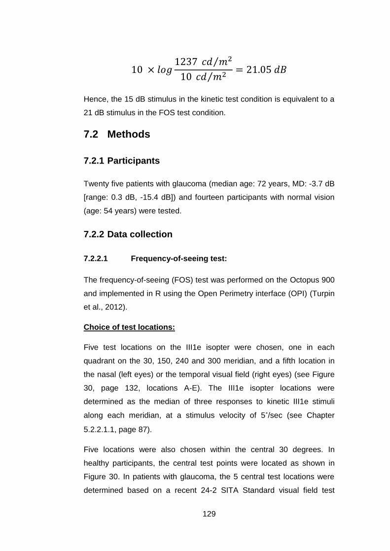
129
Hence, the 15 dB stimulus in the kinetic test condition is equivalent to a
21 dB stimulus in the FOS test condition.
7.2 Methods
7.2.1 Participants
Twenty five patients with glaucoma (median age: 72 years, MD: -3.7 dB
[range: 0.3 dB, -15.4 dB]) and fourteen participants with normal vision
(age: 54 years) were tested.
7.2.2 Data collection
7.2.2.1 Frequency-of-seeing test:
The frequency-of-seeing (FOS) test was performed on the Octopus 900
and implemented in R using the Open Perimetry interface (OPI) (Turpin
et al., 2012).
Choice of test locations:
Five test locations on the III1e isopter were chosen, one in each
quadrant on the 30, 150, 240 and 300 meridian, and a fifth location in
the nasal (left eyes) or the temporal visual field (right eyes) (see Figure
30, page 132, locations A-E). The III1e isopter locations were
determined as the median of three responses to kinetic III1e stimuli
along each meridian, at a stimulus velocity of 5˚/sec (see Chapter
5.2.2.1.1, page 87).
Five locations were also chosen within the central 30 degrees. In
healthy participants, the central test points were located as shown in
Figure 30. In patients with glaucoma, the 5 central test locations were
determined based on a recent 24-2 SITA Standard visual field test
130
(Humphrey, Carl Zeiss Meditec, CA, USA), to avoid visual field
locations with deep losses (near 0 dB).
Stimulus properties:
Two test stimulus sizes were used, Goldmann III and V, which subtend
0.43˚ and 1.73˚ of visual angle respectively (see Chapter 2.1.4.2.2,
page 45). Stimuli were presented with a duration of 200 ms. Frequency-
of-seeing was tested in separate sessions for Goldmann size III and V
stimuli with the method of constant stimuli (Urban, 1910).
Each frequency-of-seeing test session was separated into two blocks.
The first block was designed to optimize the distribution of the stimulus
contrasts used in the second block. The first block took ~10 minutes
and the second block ~20 minutes. In the second block a short break
was given after 10 minutes.
In the first block nine different stimulus contrasts were chosen and each
contrast was presented 5 times.
The results of block 1 were used to estimate an “expected contrast
sensitivity” to determine the stimulus contrasts for block 2. The data of
block 1 was fitted with a probit fitted cumulative normal function. For the
second block a different set of 8 contrasts were chosen, with each
contrast being presented 10 times. The stimulus contrasts were chosen
to lie at the 2.5th, 22.5th, 30th, 50th, 65th, 77.5th, and 97.5th percentiles of
the estimated normal distribution of responses measured in the first
block. One additional contrast was chosen to be 15 dB brighter than the
“expected contrast sensitivity” estimated in block 1 to ensure the
presence of a stimulus with a detection rate close to 100%.
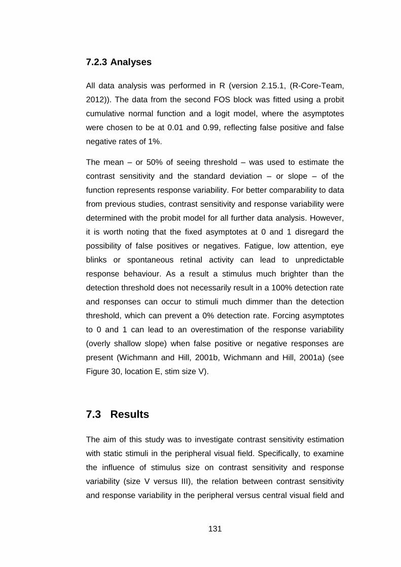
131
7.2.3 Analyses
All data analysis was performed in R (version 2.15.1, (R-Core-Team,
2012)). The data from the second FOS block was fitted using a probit
cumulative normal function and a logit model, where the asymptotes
were chosen to be at 0.01 and 0.99, reflecting false positive and false
negative rates of 1%.
The mean – or 50% of seeing threshold – was used to estimate the
contrast sensitivity and the standard deviation – or slope – of the
function represents response variability. For better comparability to data
from previous studies, contrast sensitivity and response variability were
determined with the probit model for all further data analysis. However,
it is worth noting that the fixed asymptotes at 0 and 1 disregard the
possibility of false positives or negatives. Fatigue, low attention, eye
blinks or spontaneous retinal activity can lead to unpredictable
response behaviour. As a result a stimulus much brighter than the
detection threshold does not necessarily result in a 100% detection rate
and responses can occur to stimuli much dimmer than the detection
threshold, which can prevent a 0% detection rate. Forcing asymptotes
to 0 and 1 can lead to an overestimation of the response variability
(overly shallow slope) when false positive or negative responses are
present (Wichmann and Hill, 2001b, Wichmann and Hill, 2001a) (see
Figure 30, location E, stim size V).
7.3 Results
The aim of this study was to investigate contrast sensitivity estimation
with static stimuli in the peripheral visual field. Specifically, to examine
the influence of stimulus size on contrast sensitivity and response
variability (size V versus III), the relation between contrast sensitivity
and response variability in the peripheral versus central visual field and

132
the difference between static and kinetic threshold estimates.
Frequency-of-seeing curves to size III and V stimuli at isopter locations
and in the central visual field were estimated for patients with glaucoma
and participants with normal vision. A typical example for the
frequency-of-seeing curves of an individual glaucoma patient at
different locations in the visual field is given in Figure 30.
Figure 30: Psychometric functions fitted to frequency-of-seeing data of a glaucoma patient. Test locations are indicated by letters with capital letters A-E representing the locations on the III1e isopter and small letter f-j representing central locations. Response frequencies to size III and V stimuli are depicted as filled and normal circles respectively. Psychometric functions belonging to the size III stimulus data are depicted as solid lines and as dashed lines for the size V stimulus data. Both psychometric functions fitted with a probit model and a logit model with fixed asymptotes at 0.01 and 0.99 are represented. The model with the better quality of fit is depicted as the thicker line.

133
Frequency-of-seeing curves to both size III and size V stimuli are
depicted for each test location. The position of the test locations within
the visual field is also illustrated in Figure 30. Steep slopes indicate low
response variability. The frequency-of-seeing curves to size III stimuli at
the peripheral locations A and E illustrate examples with higher
response variability. At location E the 100% detection rate was not
reached within the range of presented contrasts (Figure 30).
In patients with glaucoma the III1e isopter locations can fall within the
central visual field. This occurred in 11 out of 25 patients with
glaucoma. A total of twenty out of the 250 isopter locations were located
within the central 30˚. The data were grouped into central (≤30˚) and
peripheral (>30˚) data according to visual field eccentricity of each test
location. All data points with estimated thresholds <0 dB were excluded.
Table 7: Mean contrast sensitivity (50% of seeing threshold) and response variability (slope) for patients with glaucoma and participants with normal vision to size III and size V stimuli. Values are given for central (≤ 30˚) and peripheral test locations (> 30˚). Standard deviations are given in brackets.
Glaucoma (N=25) Normal (N=14)
Centre
(≤ 30˚)
Peri.
(> 30˚)
Centre
(≤ 30˚)
Peri.
(> 30˚)
Total Nr of locations 137 99 69 68
Eccentricity
16.15˚
(6.92)
42.98˚
(8.34)
10.95˚
(3.89)
57.20˚
(10.65)
III
50% of seeing threshold 16.79 dB
(6.79)
14.08 dB
(5.43)
28.09 dB
(3.54)
17.32 dB
(3.67)
Slope 5.94 dB
(3.77)
5.61 dB
(3.70)
1.65 dB
(1.40)
4.06 dB
(3.19)
V
50% of seeing threshold 24.69 dB
(5.95)
24.32 dB
(3.48)
33.80 dB
(1.78)
27.24 dB
(2.75)
Slope 3.43 dB
(3.20)
3.25 dB
(2.19)
1.44 dB
(1.26)
2.91 dB
(2.35)
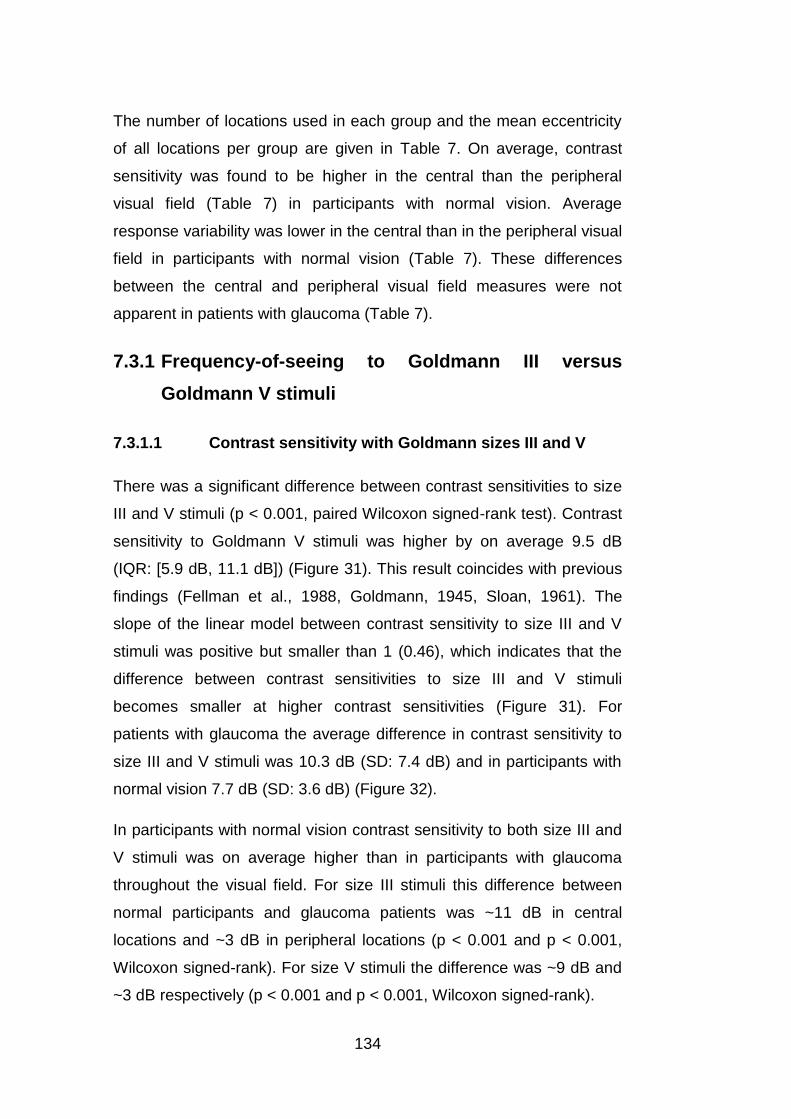
134
The number of locations used in each group and the mean eccentricity
of all locations per group are given in Table 7. On average, contrast
sensitivity was found to be higher in the central than the peripheral
visual field (Table 7) in participants with normal vision. Average
response variability was lower in the central than in the peripheral visual
field in participants with normal vision (Table 7). These differences
between the central and peripheral visual field measures were not
apparent in patients with glaucoma (Table 7).
7.3.1 Frequency-of-seeing to Goldmann III versus
Goldmann V stimuli
7.3.1.1 Contrast sensitivity with Goldmann sizes III and V
There was a significant difference between contrast sensitivities to size
III and V stimuli (p < 0.001, paired Wilcoxon signed-rank test). Contrast
sensitivity to Goldmann V stimuli was higher by on average 9.5 dB
(IQR: [5.9 dB, 11.1 dB]) (Figure 31). This result coincides with previous
findings (Fellman et al., 1988, Goldmann, 1945, Sloan, 1961). The
slope of the linear model between contrast sensitivity to size III and V
stimuli was positive but smaller than 1 (0.46), which indicates that the
difference between contrast sensitivities to size III and V stimuli
becomes smaller at higher contrast sensitivities (Figure 31). For
patients with glaucoma the average difference in contrast sensitivity to
size III and V stimuli was 10.3 dB (SD: 7.4 dB) and in participants with
normal vision 7.7 dB (SD: 3.6 dB) (Figure 32).
In participants with normal vision contrast sensitivity to both size III and
V stimuli was on average higher than in participants with glaucoma
throughout the visual field. For size III stimuli this difference between
normal participants and glaucoma patients was ~11 dB in central
locations and ~3 dB in peripheral locations (p < 0.001 and p < 0.001,
Wilcoxon signed-rank). For size V stimuli the difference was ~9 dB and
~3 dB respectively (p < 0.001 and p < 0.001, Wilcoxon signed-rank).

135
Figure 31: Contrast sensitivity for stimulus sizes III and V. Scatterplot of the estimated contrast sensitivity to size III (x-axis) versus size V stimuli (y-axis). Contrast sensitivity is higher to size V than to size III stimuli. The slope of the linear model is positive but smaller than 1 (0.46), which indicates that the difference between contrasts sensitivities to size III and V stimuli becomes smaller at higher contrast sensitivities. The relationship between contrast sensitivity to size III and V stimuli as predicted by Goldmann is indicated in grey.
The difference in contrast sensitivity to size III and V stimuli (ΔCSV,III)
correlated with visual field eccentricity in glaucoma patients
(Spearman’s rho = 0.27, p<0.001) and normal participants (Spearman’s
rho = 0.76, p<0.001) (Figure 32). The relationship between ΔCSV,III and
visual field eccentricity was significantly stronger in participants with
normal vision than in patients with glaucoma (Steiger’s z: -5.55,
p<0.001). Furthermore the slope of the linear model between contrast
sensitivity and eccentricity was steeper in the normal vision group than
in the glaucoma group (Figure 32). That means the gain in contrast
sensitivity caused by the larger stimulus area (size V) is stronger in the
peripheral than the central visual field of participants with normal vision.
In patients with glaucoma a similar gain is reached throughout the

136
visual field. The low r-squared (0.006) of the linear model in the
glaucoma group further indicates that little variance was explained by
eccentricity in the glaucoma group.
There was a significant difference in ΔCSV,III between patients with
glaucoma and participants with normal vision at central locations (≤30˚)
(Two-sample Wilcoxon signed-rank, p < 0.001), but not at peripheral
locations (>30˚) (p=0.42). This indicates that the gain in contrast
sensitivity caused by a size V stimulus differs between the glaucoma
and normal group in the central visual field, but not in the peripheral
visual field.
Table 8: Parameters of the linear models fitted to visual field eccentricity and the difference in contrast sensitivity to size III and size V stimuli (ΔCSV,III ) in patients with glaucoma and participants with normal vision.
Group N Slope: a (SE) Intercept: b (SE) R2 (p-value)
Glaucoma 236 0.04 (± 0.03) 9.33 (± 0.98) 0.006 (p=0.23)
Normal 137 0.1 (± 0.01) 4.42 (± 0.4) 0.44 (p<0.001)
Figure 32: Dependence of the change in contrast sensitivity for size III and V stimuli on visual field eccentricity. The difference in contrast sensitivity to size V and III stimuli ( ΔCSV,III ) (y-axis) is depicted against eccentricity of the test location in the visual field (x-axis). Data of participants with normal vision is on the left and data of glaucoma patients on the right. Red lines indicate the linear model fit. ΔCSV,III appeared to increase with eccentricity in both healthy participants and glaucoma patients. Parameters of the linear models are given in Table 8.
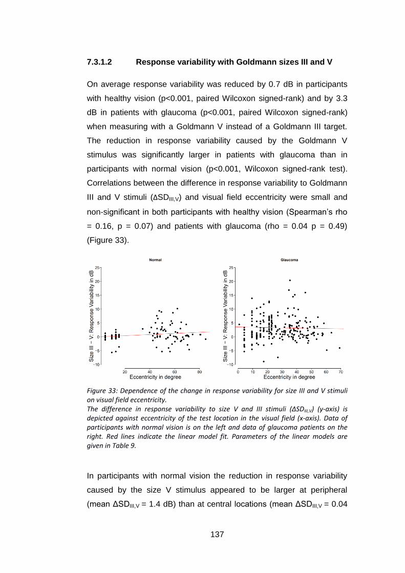
137
7.3.1.2 Response variability with Goldmann sizes III and V
On average response variability was reduced by 0.7 dB in participants
with healthy vision (p<0.001, paired Wilcoxon signed-rank) and by 3.3
dB in patients with glaucoma (p<0.001, paired Wilcoxon signed-rank)
when measuring with a Goldmann V instead of a Goldmann III target.
The reduction in response variability caused by the Goldmann V
stimulus was significantly larger in patients with glaucoma than in
participants with normal vision (p<0.001, Wilcoxon signed-rank test).
Correlations between the difference in response variability to Goldmann
III and V stimuli (ΔSDIII,V) and visual field eccentricity were small and
non-significant in both participants with healthy vision (Spearman’s rho
= 0.16, p = 0.07) and patients with glaucoma (rho = 0.04 p = 0.49)
(Figure 33).
Figure 33: Dependence of the change in response variability for size III and V stimuli on visual field eccentricity. The difference in response variability to size V and III stimuli (ΔSDIII,V) (y-axis) is depicted against eccentricity of the test location in the visual field (x-axis). Data of participants with normal vision is on the left and data of glaucoma patients on the right. Red lines indicate the linear model fit. Parameters of the linear models are given in Table 9.
In participants with normal vision the reduction in response variability
caused by the size V stimulus appeared to be larger at peripheral
(mean ΔSDIII,V = 1.4 dB) than at central locations (mean ΔSDIII,V = 0.04

138
dB) (Two-sample Wilcoxon signed-rank: p=0.02). This was not the case
in patients with glaucoma (p=0.82). The mean ΔSDIII,V of glaucoma
patients in the central and peripheral visual field was 3.4 dB and 3.2 dB
respectively.
Table 9: Parameters of the linear models fitted to visual field eccentricity and the difference in contrast sensitivity to size III and size V stimuli (ΔSDIII,V) in patients with glaucoma and participants with normal vision
Group N Slope: a (SE) Intercept: b (SE) R2 (p-value)
Glaucoma 236 -0.01 (± 0.02) 3.56 (± 0.76) -0.004 (p=0.71)
Normal 137 0.02 (± 0.01) 0.04 (± 0.39) 0.03 (p=0.03)
7.3.2 Relation between response variability and
sensitivity in the central versus peripheral visual
field
Response variability (SD) was found to increase as contrast sensitivity
decreases (Figure 34). The data collected with Goldmann size III stimuli
was compared to previous findings by Henson et al. (Henson et al.,
2000) (Figure 34). Henson et al. measured frequency-of-seeing curves
in participants with normal vision, glaucoma, ocular hypertension and
optic neuritis. They found a similar relationship between response
variability and contrast sensitivity independent of the visual disorder
(Figure 34).
Both our and Henson et al.’s data were fitted with a linear model
loge(SD) = a*sensitivity + b. The slope of the models for this data set
and Henson et al.’s data appeared similar (Figure 34) (Table 10).
The linear model described Henson et al.’s data better than the current
data. Residual standard errors were 0.37 and 0.63, respectively. While
the relation between log(SD) and sensitivity appears linear in Henson’s
data, our data appeared to asymptote at low sensitivity (Figure 34).
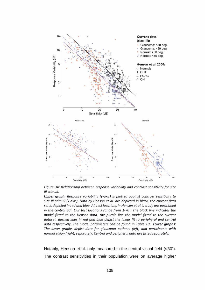
139
Henson et al, 2000:
Current data
(size III):
Figure 34: Relationship between response variability and contrast sensitivity for size III stimuli. Upper graph: Response variability (y-axis) is plotted against contrast sensitivity to size III stimuli (x-axis). Data by Henson et al. are depicted in black, the current data set is depicted in red and blue. All test locations in Henson et al.’s study are positioned in the central 30˚. Our test locations range from 1-70˚. The black line indicates the model fitted to the Henson data, the purple line the model fitted to the current dataset, dashed lines in red and blue depict the linear fit to peripheral and central data respectively. The model parameters can be found in Table 10. Lower graphs: The lower graphs depict data for glaucoma patients (left) and participants with normal vision (right) separately. Central and peripheral data are fitted separately.
Notably, Henson et al. only measured in the central visual field (≤30˚).
The contrast sensitivities in their population were on average higher

140
than in our population and were all higher than 10 dB. Thus the trend to
asymptote at lower sensitivities might not be detectable in Henson’s
data. Our data had a lower intercept, which hints at consistently lower
response variability at any sensitivity compared to Henson et al.’s data.
By tendency, peripheral locations appeared to have a slightly lower
response variability than central locations with respect to contrast
sensitivity, this is especially prominent in participants with normal vision
(see Figure 34, red data points).
Table 10: Parameters of the linear models between contrast sensitivity and response variability to size III stimuli in Henson et al.’s data and patients with glaucoma and participants with normal vision
Group N Slope: a (SE) Intercept: b (SE) R2 (p-value)
Henson et
al. 71 -0.08 (± 0.004) 3.27 (± 0.13) 0.57 (p<0.001)
Combined 373 -0.08 (± 0.005) 2.70 (± 0.09) 0.46 (p<0.001)
Central
(≤30˚) 206 -0.09 (± 0.12) 2.93 (± 0.006) 0.55 (p<0.001)
Peripheral
(>30˚) 167 -0.07 (± 0.15) 2.57 (±0.009) 0.29 (p<0.001)
Normal 137 -0.09 (± 0.007) 2.67 (± 0.17) 0.51 (p<0.001)
Glaucoma 236 -0.06 (± 0.007) 2.528 (± 0.12) 0.28 (p<0.001)
Normal
(≤30˚) 69 -0.11 (± 0.02) 3.31 (± 0.64) 0.25 (p<0.001)
Normal
(>30˚) 68 -0.13 (± 0.02) 3.32 (± 0.36) 0.37 (p<0.001)
Glaucoma
(≤30˚) 137 -0.07 (± 0.01) 2.72 (± 0.16) 0.32 (p<0.001)
Glaucoma
(>30˚) 99 -0.06 (± 0.01) 2.33 (± 0.16) 0.21 (p<0.001)
The frequency-of-seeing data set to Goldmann size V stimuli showed a
similar overall relationship between contrast sensitivity and response
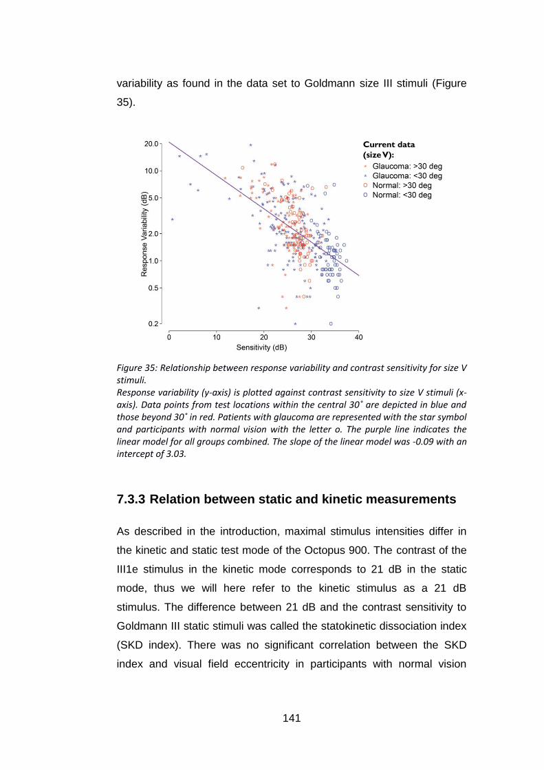
141
variability as found in the data set to Goldmann size III stimuli (Figure
35).
Current data
(size V):
Figure 35: Relationship between response variability and contrast sensitivity for size V stimuli. Response variability (y-axis) is plotted against contrast sensitivity to size V stimuli (x-axis). Data points from test locations within the central 30˚ are depicted in blue and those beyond 30˚ in red. Patients with glaucoma are represented with the star symbol and participants with normal vision with the letter o. The purple line indicates the linear model for all groups combined. The slope of the linear model was -0.09 with an intercept of 3.03.
7.3.3 Relation between static and kinetic measurements
As described in the introduction, maximal stimulus intensities differ in
the kinetic and static test mode of the Octopus 900. The contrast of the
III1e stimulus in the kinetic mode corresponds to 21 dB in the static
mode, thus we will here refer to the kinetic stimulus as a 21 dB
stimulus. The difference between 21 dB and the contrast sensitivity to
Goldmann III static stimuli was called the statokinetic dissociation index
(SKD index). There was no significant correlation between the SKD
index and visual field eccentricity in participants with normal vision

142
(Spearman’s rho = -0.14, p = 0.24) and patients with glaucoma (rho = -
0.07, p = 0.46) (Figure 36).
Figure 36: Statokinetic dissociation versus visual field eccentricity. Relationship between visual field eccentricity and the SKD index, which indicates the difference between kinetic and static contrast sensitivity at each location. There was no significant correlation between the SKD index and eccentricity. Interestingly, the three points measured within the central 5 degree (macula) had SKD indices close to 0 dB., this is in line with findings in previous literature (Fankhauser and Schmidt, 1960).
On average, contrast sensitivity to size III static stimuli was lower than
21 dB [median (m): 16.6 dB, 90% interval: 6.2 dB, 20.9 dB]. Our data
showed no apparent differences in the median contrast sensitivity
depending on the test meridian (Figure 37). Differences between
healthy observers and glaucoma patients were small (Figure 37) with
glaucoma patients being slightly less sensitive to the static stimulus.

143
Figure 37: Estimated contrast sensitivity (probit model) on isopter locations to size III stimuli compared to the kinetic stimulus contrast (21 dB). On the left hand side the five isopter locations are represented separately. On the right hand side glaucoma patients and participants with healthy vision are depicted separately. The small circles represent single contrast sensitivities of each subject at each location. Box plots give the inter quartile range with whiskers representing the 90% range.
7.4 Discussion
7.4.1 Influence of stimulus sizes (III and V) on contrast
sensitivity and response variability
In this chapter the following questions regarding stimulus size were
posed: How does the choice of a stimulus V instead of III affect contrast
sensitivity and response variability? Is this affected by the eccentricity in
the visual field? On average, there was an increase of contrast
sensitivity by 10 dB when using size V stimuli and a reduction in
response variability by 2 dB. The difference in contrast sensitivity to size
III and V stimuli increased with visual field eccentricity. These findings
were in agreement with previous studies (Wilson, 1970, Dannheim and
Drance, 1971, Wald, 1938, Redmond et al., 2010) and match the
predictions of a theory that connects the change in contrast sensitivity
caused by a change in stimulus size to ganglion cell density (Wilson,
1970, Swanson et al., 2004, Fischer, 1973, Anderson, 2006): Density of
144
retinal ganglion cells decreases with visual field eccentricity. A larger
area has to be covered to stimulate an equivalent number of ganglion
cells in the peripheral visual field compared to the central field. Up to a
certain number of responding retinal ganglion cells, and respectively up
to a certain increase in stimulus area a constant gain in contrast
sensitivity occurs. After that number and respective area is reached the
gain in contrast sensitivity becomes lower. Thus, in a location with low
ganglion cell density an increase in stimulus area can have a stronger
effect than in a location with high ganglion cell density. In glaucoma,
ganglion cell density is reduced. Consequently, a larger gain in contrast
sensitivity related to an increase in stimulus area is expected
throughout the visual field in glaucoma.
In line with this theory, the results showed a gain in contrast sensitivity
and a reduction in response variability in peripheral locations in
participants with normal vision and throughout the visual field in patients
with glaucoma. This gain in contrast sensitivity and reduction in
response variability was considerably smaller in the central visual field
of participants with normal vision.
The difference in contrast sensitivity to the two stimulus sizes was found
to increase with visual field eccentricity in participants with normal
vision. Thus the same reduction in stimulus area required a stronger
increase in stimulus contrast in the peripheral visual field than in the
central visual field to still be detected. This corroborates previous
findings that Ricco’s area increases with eccentricity (Wilson, 1970,
Redmond et al., 2010, Swanson et al., 2004, Fischer, 1973). In the
central visual field Ricco’s area is already covered with a size III
stimulus. There, an increase in size results in incomplete spatial
summation, which leads to a lower gain of contrast sensitivity. The
further a location is in the eccentricity, the wider is the range during
which complete spatial summation occurs and the higher is the potential
gain in contrast sensitivity.

145
The overall increase in contrast sensitivity to size V stimuli in patients
with glaucoma indicates that the dynamic range could be increased by
the use of a size V stimulus in perimetric tests for patients with
glaucoma. Wall et al. showed that the dynamic range increases by
about 1 log unit when using size V instead of size III stimuli in standard
automated perimetry (Wall et al., 2010, Wall et al., 2008). However, the
use of size V stimuli in the central visual field might not be a good
choice in tests that focus on the detection of glaucoma. In general it
might not be advisable to use a stimulus size that is larger than Ricco’s
area at any given location of the healthy visual field, when it comes to
detection of glaucoma. In a healthy location the larger stimulus area
would not lead to a strong gain in contrast sensitivity. However, in an
abnormal location, where ganglion cell density is decreased and thus
Ricco’s area is increased a large gain in contrast sensitivity would
occur. Thus in central visual field tests with size V stimuli, it would be
more difficult to distinguish abnormal from normal contrast sensitivities.
Since the gain in contrast sensitivity to size V compared to size III
stimuli is large in peripheral locations of the normal visual field, this
problem would not arise to the same extent in the periphery and size V
stimuli might be suitable in the peripheral visual field.
While a test with stimulus size V in the central visual field might not be
helpful for diagnosis, it could, however, be useful for monitoring of the
disease. The increase in contrast sensitivity caused by the larger size V
stimulus could increase the dynamic range and the lower response
variability could yield more reliable contrast sensitivity estimates.
Therefore it could be beneficial to have different tests for first detection
and for monitoring in later stages of disease. For detection either stimuli
that are consistently smaller than the respective Ricco’s area in the
normal visual field or stimuli that match Ricco’s area at each location
could be useful for detection. This would prevent that the gain in
contrast sensitivity, caused by additional complete summation at low

146
RGC locations, masks visual field deficits in glaucoma. For monitoring
of the progression of glaucoma at a later stage larger stimulus sizes
that increase the dynamic range and reduce response variability could
be useful (Wall et al., 2008, Wall et al., 2013, Wall et al., 1997).
7.4.2 Response variability to static stimuli in the central
versus peripheral visual field
The results showed that response variability increases with decreasing
contrast sensitivity. This relationship appeared similar to the relationship
predicted by Henson et al. (Henson et al., 2000). Other studies also
found a similar increase of response and measurement variability with
decreasing contrast sensitivity (Weber and Rau, 1992, Chauhan et al.,
1993, Olsson et al., 1993, Russell et al., 2012a, Artes et al., 2002).
While the slope of the relationship between contrast sensitivity and
response variability was almost identical in our data as in Henson et
al.’s, we found a consistent shift which suggested that response
variability with respect to contrast sensitivity was generally lower than
found by Henson et al. This shift could be due to due to differences in
the settings of the perimeters used in the two studies. Henson et al.’s
data were collected on a Henson 4000 perimeter. The Henson 4000
perimeter has a different maximal stimulus intensity (1000 cd/m2) than
the Octopus 900 (1237 cd/m2). A constant of 1 dB has to be added to
achieve the same stimulus luminance on the Henson 4000 perimeter as
on the Octopus 900. Therefore, the difference in maximal stimulus
intensity cannot explain the shift between these data and Henson et
al.’s data. Correcting for the maximal stimulus intensity would actually
further increase the effect. The Henson 4000 perimeter also uses a
lower background luminance (3.14 cd/m2) (Henson, 2007) than the
Octopus 900 (10 cd/m2). Fellman et al. found that a decrease in
background illumination from 10 cd/m2 to 1 cd/m2 led to an increase in
147
detection threshold by about 5 dB (Fellman et al., 1988). Thus the lower
background luminance, which leads to higher contrasts, in Henson et
al.’s study might contribute to the difference found between Henson et
al.’s and our data.
The linear fit between contrast sensitivity and the logarithmically scaled
response variability was less suitable in this data set than in Henson et
al.’s data. The response variability appears to asymptote at higher
contrast sensitivities. This effect is not apparent in Henson et al.’s data.
However, as they measured only within the central 30˚, contrast
sensitivities were generally higher. This tendency might also have
occurred at higher contrast sensitivities in their data.
By tendency, response variability at peripheral locations appeared to be
lower with respect to contrast sensitivity than at central locations. This
was especially the case in participants with normal vision. This
suggests that the relationship between contrast sensitivity and response
variability depends on visual field eccentricity. Thus, measurements of
contrast sensitivity in the peripheral field may be possible with greater
precision than one would suggest from Henson et al.’s model.
7.4.3 Relation between static and kinetic measurements
We found a higher sensitivity to kinetic stimuli than to static stimuli. On
average there was a difference of 4.4 dB. However, overall, the
difference between the kinetic and static measures was highly variable.
Thus while on average we can relate between the two measures by
adding a constant, it has to be noted that the prediction of the shift is
imprecise. A factor that might add to the variability in the difference
between kinetic and static thresholds is the response criterion used.
The level of uncertainty for detecting a stimulus may vary, leading to
changes in the measure threshold. In contrast to forced choice tasks,
148
both the kinetic and static perimetric “yes or no” tasks do not allow
control of the response criterion (Treutwein, 1995, Harvey, 1986).
Moreover, the different nature of the static and kinetic tasks might
influence the response criteria of participants. In the kinetic task a
stimulus is moved from “non-seeing” to “seeing” areas, thus the
probability of detection increases over time. In terms of the participant’s
perception, this could be regarded as similar to the ascending method
of limits in which the stimulus intensity is gradually raised, thus
increasing the probability of detection over time. Here, a participant
might be more inclined not to respond until he or she is more certain,
resulting in a conservative response criterion. The static test in this
study was performed with the method of constant stimuli. That means
static stimuli of different intensities are presented in a random order and
the probability of detection does not change over time. As the response
criterion may vary between individuals, between tasks, and even within
individuals within the same task, it might very well contribute to the
variability of the differences between static and kinetic thresholds found
in the current data.
Only one kinetic stimulus was used in this study, the III1e stimulus, the
dissociation of on average 4.4 dB might be different for other stimulus
sizes and contrasts. However, Hudson and Wild found similar
dissociations of between 4 and 5 dB for a wide range of Goldmann
stimuli (size I with filters 4d, 3b, 2e, 2c, 2a, 1e and 1d; and size III with
filters: 4e, 4c, 3e, 3d, 3c and 3b) (Hudson and Wild, 1992).
There was no significant correlation between the difference in static and
kinetic sensitivity and visual field eccentricity. Interestingly, the three
points measured within the central 5 degrees (macula) had differences
between kinetic and static sensitivity close to 0 dB, this is in line with
findings in previous literature (Fankhauser and Schmidt, 1960, Hudson
and Wild, 1992). The difference between kinetic and static sensitivity
also did not seem to depend on the meridians located in different

149
quadrants of the visual field. This agrees with previous findings by
Hudson and Wild who also found statokinetic dissociation to be largely
independent of eccentricity and meridian (Hudson and Wild, 1992).
The properties of kinetic and static measures differ. In one technique
the location of detection is estimated and in the other threshold
sensitivity is estimated at specific locations. However, on average there
appears to be a similar difference between kinetic and static
sensitivities independent of meridian and eccentricity. My findings and
findings by Hudson and Wild indicated that the same constant can be
added to relate between static and kinetic thresholds for Goldmann
stimulus sizes I and III (Hudson and Wild, 1992). It is still unclear
whether this also applies to larger stimulus sizes (e.g. Goldmann
stimulus V). Moreover, it is still unknown what causes the high
variability of the differences between static and kinetic thresholds.
In the previous chapters I explored the feasibility of automated kinetic
perimetry in the peripheral visual field. The results suggest that, in
automated kinetic perimetry, repeated presentations are necessary to
gain sufficient precision of the location estimates, thus the automated
measurement of several isopters to examine the entire visual field, as
e.g. done in Goldmann perimetry might be too time consuming. Static
automated perimetry has been shown to be an efficient method in the
central visual field. However, the large number of locations required to
cover the entire visual field would lead to long test durations. A
promising technique to examine the entire visual field could be a
combination of static and kinetic perimetry, wherein the isopter
establishes a “region of interest” within which a pattern of locations is
tested with static perimetry. Since kinetic and static measures appear to
be relatable to some extent, both static and kinetic visual fields could be
compared and combined into a common test.

150
8. Using eye tracking to assess
reading performance in patients
with glaucoma: A within-person
study
8.1 Introduction
The conventional view of vision loss in glaucoma suggests disruption of
peripheral vision and minimal impact on tasks that require good central
vision, like reading. However, as previously described in Chapter 4,
patients with glaucoma regularly self-report difficulties with reading
(Crabb et al., 2013, Nelson et al., 1999, Aspinall et al., 2008,
Viswanathan et al., 1999, Freeman et al., 2008). Furthermore, evidence
is emerging from experimental studies showing that patients with
glaucoma have impaired reading performance when compared to their
visually healthy peers. Theses impairments are particularly evident for
patients with advanced or bilateral visual field loss (Fujita et al., 2006,
Ramulu, 2009, Ishii et al., 2013); when reading small size text
(Altangerel et al., 2006); when reading text at low contrast (Burton et al.,
2012); or when reading for sustained periods of time (Ramulu et al.,
2013). However, not all patients displayed reduced reading speeds in
these studies, with some patients appearing to be much more affected
than others. A limiting feature of the studies that have generated these
results is that reading speed, as an experimental outcome measure, is
subject to much between-person variability: it is very difficult to isolate
the impact of the glaucoma visual field loss from all the other factors,
such as age, visual acuity, and cognitive and reading ability, that might
contribute to slower reading. Furthermore, differences in eye movement
patterns may also influence reading speed. Eye movements

151
supplement information about how long a person takes to read, by
giving insight into how they are reading. Previous research has
considered eye movements in patients with glaucoma compared to
visually healthy controls when carrying out a number of other visual
tasks, such as visual search (Smith et al., 2012b), face recognition
(Glen et al., 2013), viewing of photographs (Smith et al., 2012a), and
watching of driving videos (Crabb et al., 2010). In these studies,
patients sometimes displayed different eye movement patterns on
average to controls, although it was suggested that some patients may
“adapt” their eye movements in ways that enable them to function better
in the task (Glen et al., 2013, Smith et al., 2012b). However, the case-
control design that featured in all these studies again made it difficult to
discern the nature of the contribution of visual field loss to changes in
eye movement behaviour.
As yet no studies have considered performing a within-person, or
between-eye, reading study to examine the impact of glaucoma visual
field loss on reading performance: the idea here would be that a more
damaged eye could be compared with a less affected fellow eye. An
experimental design such as this might proffer advantages over studies
comparing patients to controls, where large numbers of people are
needed to demonstrate effects. In addition, experimental studies of
reading speed in glaucoma have been constrained to those where
reading “out loud” or timed silent reading is simply the main, or only,
outcome measure. One recent study incorporated eye tracking when
investigating reading performance in glaucoma (Cerulli et al., 2014): the
findings of that case-control study, which measured the maximum and
minimum sizes of eye movements made during a reading task by
patients compared to controls, hinted that glaucoma may lead to some
alterations in fixation behaviour. However, to date, no studies have
used an eye tracker to measure more task-specific saccades (i.e., rapid
eye movements occurring between locations on the text) to tease out
152
the effects that might result from glaucomatous visual field loss whilst
reading short passages of text.
In this chapter, I explore the usefulness of comparing monocular
reading performance in patients with asymmetric glaucomatous visual
field loss. The study measures reading performance using eye-tracking
whilst participants silently read very short passages of text. My main
hypothesis is that patients will take longer to read short passages of text
in what is considered to be their worse eye (most visual field damage)
when compared to their better eye (least visual field damage); I aimed
to do this in just a small sample of patients in order to demonstrate the
effectiveness of the experimental design. I also, as a secondary aim,
tested the idea of determining different types of reading-specific
saccadic eye movements, in an automated fashion, specifically eye
movements that occur in a forward direction (forward saccades),
saccades that “backtrack” over previously read text (regressions), those
that occur between the end of one line and the beginning of the next
(line change saccades), and eye movements that do not fit expected
patterns (unknown saccades). Next I investigated if any of these
measurements from this automated approach are associated with the
size of between-eye deficits in standard measures of visual function. In
the context of this thesis, this study illuminates the difficulty of
assessing patient performance in everyday tasks.
The results of this study have been previously published in the Journal
of Ophthalmology (Smith et al., 2014). ND Smith, VM Mönter and DP
Crabb designed the study. Patients were recruited by VM Mönter. All
testing was done by VM Mönter. The model for classification of eye
movement types was written by ND Smith, who also pre-processed the
eye movement data. The data analysis was chiefly done by ND Smith.
The final paper was written jointly by all the authors.
153
8.2 Methods
8.2.1 Participants
Participants were recruited from a database of patients that had taken
part in previous studies conducted at City University London (Smith et
al., 2012b, Glen et al., 2012). All patients had a clinical diagnosis of
primary open angle glaucoma and had no other ocular diseases.
Patients were contacted if they had previously presented with
asymmetric visual field loss between eyes as measured using a central
24-2 SITA Standard Test on the Humphrey Visual Field Analyzer (HFA,
Carl Zeiss Meditec, CA, USA). This was quantified by considering the
HFA mean deviation (MD); this summary measure expresses the
average reduction in the visual field relative to a group of visually
healthy age-matched observers (Artes et al., 2011). Participants were
only invited into the study if the MD differed by more than 6dB between
eyes. This value represents a clinically significant difference as used in
staging schemes for visual field severity (Hodapp et al., 1993).
The study was approved by the Ethics Committee for the School of
Health Science, City University London. All participants gave their
informed consent and the study conformed to the Declaration of
Helsinki.
8.2.2 Standard vision testing
Fourteen patients were recruited and all testing was carried out on one
day. Visual acuity (VA) as measured with the Early Treatment Diabetic
Retinopathy (ETDRS) chart and contrast sensitivity as measured with
the Pelli-Robson chart (PR Log CS) were assessed monocularly.
Astigmatic error was less than ±2.5 dioptres in all those recruited.
Visual field tests (central 24-2 and 10-2 SITA Standard) were conducted
in each eye using a HFA. On testing (central 24-2), two of the 14
patients had a between eye MD difference of less than 6 dB (4.7 and

154
4.8 dB). From this point the patient’s eye with the worse visual field
damage (worse MD) is referred to as the “worse eye” and the fellow eye
as the “better eye”.
8.2.3 Experimental setup and eye-tracking
The reading experiment was performed on a 56 cm CRT computer
monitor displaying at a resolution of 1600 by 1200 pixels and a refresh
rate of 100 Hz (Iiyama Vision Master PRO 514, Iiyama Corporation,
Tokyo, Japan). Participants were seated (with a head rest) in front of
the computer screen. Each participant was fitted with a set of trial
frames with the appropriate refractive correction. One eye was
randomly selected then occluded by inserting a blackout lens into the
trial frames. Participants were then presented with 50 different texts
(trials) on the screen, one at a time, and were asked to silently read
them, “as quickly and accurately as possible”. Once the participant had
read the 50 texts, they had a short break before repeating the task
using their alternate eye with 50 novel texts. Participants read the same
100 texts but in a randomised order. Each text consisted of one
sentence, distributed over two lines, using the “Courier New” font at size
38 in which each letter subtended a maximum height of 0.75° visual
angle and a constant width of 0.6°. The standardised passages of text
had an average Flesch-Kincaid readability score of 4.6 and were the
same as those used by Kabanarou and Rubin (Kabanarou and Rubin,
2006). The background brightness was 33.4 cd/m2 and the text was
displayed at 0.04 cd/m2. Each paragraph subtended 21° width and 3° in
height.
Eye movements were recorded simultaneously during the reading task
using an EyeLink 1000 (SR Research Ltd., Mississauga, Ontario,
Canada) which was set to record the participant’s eye location at 1000
Hz. It is claimed that the EyeLink 1000 measures at an average
accuracy of better than 0.5°. The saccade detection thresholds were

155
defined by a velocity greater than 30°/s and acceleration above
8000°/s2. Before the study commenced, a calibration was performed
and had to be classified as of a “good” standard as set by the
instrument. Furthermore, between each trial (each displayed sentence)
a drift check was performed and, if a substantial drift had occurred, a
recalibration would be carried out.
8.2.4 Analysis of Eye-Tracking data
To prepare the eye movement data for analysis, a novel preprocessing
technique was developed. These methods adjusted for calibration
errors in the eye tracking and ensured that only those saccades
relevant to the reading task were included. Secondly, a novel method
was designed that automatically classifies reading-specific eye
movements according to their saccade type, that is, whether they
occurred from left to right (forward saccade), right to left (regression), or
between lines (line change) or did not conform to expected reading
patterns (unknown saccade). These methods might also be useful
techniques in future studies using eye tracking to measure reading
performance. The techniques described below do not require
information about the specific content of the underlying text, such as
details of the words and characters, but only the locations of the start
and end of the text.
8.2.4.1 Preprocessing
Data from the eye-tracker was used to determine reading duration for
each trial in addition to identifying the key eye movement patterns made
whilst reading the texts. The eye tracker was running before the display
of each text in order to ensure that all eye movements were recorded,
meaning it was highly likely that some additional eye movements were
made prior to beginning to read each sentence that were irrelevant to
the task. Furthermore, the drift correction carried out before each trial
meant that the participant always began the trial by fixating in the

156
middle of the screen, therefore introducing bias into subsequent eye
movement recordings. It was therefore necessary to pinpoint the exact
points at which the person actually began reading the sentence and the
point at which they finished reading. Use of an automatic real-time start
and end point has the potential to misidentify when the person started
or finished reading, as this technique uses fixed points on the screen
and therefore assumes perfect calibration of the eye-tracker. To
address this issue, a novel ‘”preprocessing” method was therefore
implemented. Some example preprocessed scanpaths are shown in
Figure 38(a), showing additional saccades that occurred before and
after the patient read the passage.
The first stage of the preprocessing algorithm attempted to correct any
rotational errors in the eye movement data. As the text was displayed
centrally, small errors in edge calibration were not of huge concern for
this particular task; however inspection of scanpaths revealed that data
sometimes appeared to be rotated along the centre. To correct for this,
it was assumed that all small saccades running ±20° along the
horizontal (approximation of reading between words) should be
corrected to correspond with the angle of the text (average angle of
horizontal or 0°). Therefore, the circular median of all these ±20° angles
of the saccades was calculated per trial, and all saccades were rotated
(corrected) by this amount. Visual analysis of scanpaths also confirmed
that, on being first presented with a text, participants sometimes made
several involuntary eye movements at locations on the screen that were
irrelevant to the task itself, before adjusting their gaze position so that
they could start reading from the beginning of the sentence. In order
that the analysis would only include those eye movements that were
relevant to the task, an automated procedure was developed that
determined which eye movements coincided with the text’s start and
end location, thereby filtering out all other irrelevant eye movements.
This process involved a series of steps to identify the start and end
point locations signalling the start and end point of reading each text.

157
The standard preset SR Research EyeLink parser (edf2asc) results in
sharp downward movements being recorded at the point just before the
pupil disappears (i.e., during a blink). Sharp downward saccades do not
correspond with reading, so these were identified and excluded
specifically any saccade with an amplitude >6˚ and with an angle of
between 250˚ and 290˚. Next, the aim was to detect the starting point of
the saccade nearest to the first word of the text and the end point of the
saccade closest to the final word of the text. However, this procedure
was complicated by the fact that the text was rectangular in shape, with
the height being substantially smaller in size than the width, a factor that
would bias end point detection. For instance, the end point of a saccade
made at the end of the first line of text (i.e., top right of the text) could
be incorrectly classified as being nearer to the end of the text than a
saccade made on the line below. Therefore the locations of the saccade
start and end points were normalised in order to make the axes equal.
Specifically, the Euclidian distance from (0, 0) (top left) for each
saccade start point and the distance from (1, 1) (bottom right) for each
saccade end point were calculated, creating two sets of distances. An
exponential weighting was applied to these two sets of distances. As
such, the more the distance value increases the further the point is from
the start location. The start saccade was then selected as the minimum
distance from (0, 0) once the weights have been applied. The purpose
of this procedure was to “encourage” the algorithm to select the first
element in the set as the start of the sentence; however if, for example,
the distance of the first saccade’s start point is larger than another
saccade, the smallest distance from (0, 0) will be selected to be the
start point. To select the end point, the same process is applied to the
saccade end points, except that the weights are reversed to
“encourage” the algorithm to choose the final value. An example of this
process can be seen by viewing Figure 38, Participant 1: when viewing
the raw scanpath in column (a) and the processed path in column (b), it
can be observed that two points are a similar distance from (0, 0). Using

158
the weighting, the algorithm is “encouraged” to choose the earlier point
as the cut-off.
The reading duration was then defined as the time between the start of
the first saccade and the end of the final saccade (the rotation and the
reading extraction stages are shown in Figure 38(b). Once this was
complete, any trial shorter than 500 ms or less than 2 saccades per
second was excluded as it is likely the trial was of poor quality.
Figure 38: Four examples of reading scanpaths from four different glaucoma patients with their visual fields on the left. The start and end of each saccade are represented by a circle. Column (a) shows the original scanpaths made by the four participants reading the text. Column (b) shows the scanpath after the rotation has been corrected and reading-specific saccades have been extracted using the preprocessing algorithm. Column (c) shows the scanpath results from the clustering and classification algorithm.The number represents the order in which the saccades occurred, and the colours represent the classification that was attributed to them by the automated clustering algorithm (blue: forward saccade, green: between line saccade, red: regression, and brown: unknown).

159
8.2.5 An automated algorithm for classifying the reading
eye movements
Eye-tracking software typically expresses data with general measures,
such as the size (amplitude) or location of each saccade. However, in
tasks such as reading, the properties of each saccade will vary
according to the demands of the task. For instance, when reading, a
person will make small forward saccades (from left to right). It is also
common for people to “backtrack” to reread previous sections (referred
to as a “regression”). The properties of a saccade occurring between
the end of one line and the beginning of the line below “line change” will
again differ. Finally, readers may also make saccadic eye movements
that do not conform to expected patterns (unknown). For this
experiment an automated data analysis algorithm was developed for
classifying the types of saccade made during the task. This method
might also be of use in other eye-tracking experiments. At the centre of
this technique is a Gaussian mixture model (GMM) that mines for
clusters in the data. This approach was only possible due to the type of
texts used, where line length was consistent throughout, giving
predictable expected saccade angles and similar amplitudes per
person. Specifically, the information needed to classify the eye
movements is the amplitude (in degrees) of each saccade and the
angle of each saccade, for all 50 sentences (trials) read by the “better
eye” in each person. Next, it is necessary to acknowledge that the angle
of eye movements occurring in a forward direction (from left to right) will
occur at an average of 0˚; for example, some forward saccades could
occur at 340˚ and others at 20˚. The discrepancy between these values,
whilst indicating the same saccade type, will subsequently influence the
success of the classification algorithm by yielding two separate clusters
that actually give the same information. To avoid having to use circular
statistics to compensate for such a scenario, all angle values were
adjusted by −90˚, meaning that standard statistical methods could be
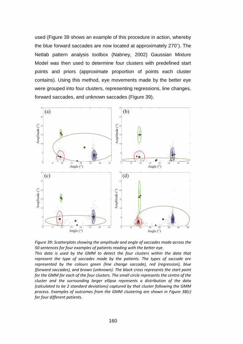
160
used (Figure 39 shows an example of this procedure in action, whereby
the blue forward saccades are now located at approximately 270˚). The
Netlab pattern analysis toolbox (Nabney, 2002) Gaussian Mixture
Model was then used to determine four clusters with predefined start
points and priors (approximate proportion of points each cluster
contains). Using this method, eye movements made by the better eye
were grouped into four clusters, representing regressions, line changes,
forward saccades, and unknown saccades (Figure 39).
Figure 39: Scatterplots showing the amplitude and angle of saccades made across the 50 sentences for four examples of patients reading with the better eye. This data is used by the GMM to detect the four clusters within the data that represent the type of saccades made by the patients. The types of saccade are represented by the colours green (line change saccade), red (regression), blue (forward saccades), and brown (unknown). The black cross represents the start point for the GMM for each of the four clusters. The small circle represents the centre of the cluster and the surrounding larger ellipse represents a distribution of the data (calculated to be 2 standard deviations) captured by that cluster following the GMM process. Examples of outcomes from the GMM clustering are shown in Figure 38(c) for four different patients.

161
Data yielded when reading with the worse eye was then classified in the
same way, so that the proportion of saccades that fell into each of the
four clusters could be calculated and compared.
8.2.6 Data analysis
A linear mixed effects ANOVA was performed in R (version 2.15.1, (R-
Core-Team, 2012)) using the linear and non-linear mixed effects
models (nlme) package to assess the reading duration per trial and
saccade rate between patients’ worse and better eyes. A mixed effects
model was chosen since different sentences were viewed by the worse
and better eye. The random effect was set as the patient. The ANOVA
was performed to test the null hypothesis, for each response, that the
means for the patients’ worse and better eyes are the same.
For each eye the percentage of eye movements were calculated that
were automatically classed as the four types of saccade by the
classification algorithm, namely, “forward saccades,” “regressions
(backwards saccades),” “between line (line change) saccades,” and
“unknown” across the 50 trials read by the better and worse eye,
respectively. Statistical differences in these proportions between the
worse and better eye were then assessed (Wilcoxon’s test).
To investigate whether the magnitudes of the change in the key
measured variables between eyes for each person were important, the
difference between eyes for reading duration and saccade rate (worse
eye minus better eye) was calculated next to create novel “change”
variables for each person. The differences between the worse and
better eye were also calculated for all the measured visual function
parameters (i.e., change in visual field severity, VA, and CS between
eyes) and then each of these resulting variables was compared to the
changes in reading duration and saccade rate between eyes.
Therefore, it could be determined whether larger reductions in visual
field defect severity, contrast sensitivity, or visual acuity were related to
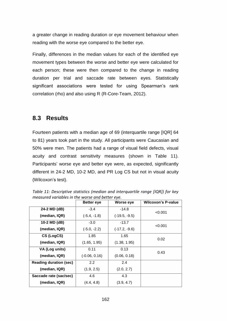
162
a greater change in reading duration or eye movement behaviour when
reading with the worse eye compared to the better eye.
Finally, differences in the median values for each of the identified eye
movement types between the worse and better eye were calculated for
each person; these were then compared to the change in reading
duration per trial and saccade rate between eyes. Statistically
significant associations were tested for using Spearman’s rank
correlation (rho) and also using R (R-Core-Team, 2012).
8.3 Results
Fourteen patients with a median age of 69 (interquartile range [IQR] 64
to 81) years took part in the study. All participants were Caucasian and
50% were men. The patients had a range of visual field defects, visual
acuity and contrast sensitivity measures (shown in Table 11).
Participants’ worse eye and better eye were, as expected, significantly
different in 24-2 MD, 10-2 MD, and PR Log CS but not in visual acuity
(Wilcoxon’s test).
Table 11: Descriptive statistics (median and interquartile range [IQR]) for key measured variables in the worse and better eye.
Better eye Worse eye Wilcoxon’s P-value
24-2 MD (dB)
(median, IQR)
-3.4
(-5.4, -1.8)
-14.8
(-19.5, -9.5) <0.001
10-2 MD (dB)
(median, IQR)
-3.0
(-5.0, -2.2)
-13.7
(-17.2, -9.6) <0.001
CS (LogCS)
(median, IQR)
1.85
(1.65, 1.95)
1.65
(1.38, 1.95) 0.02
VA (Log units)
(median, IQR)
0.11
(-0.06, 0.16)
0.13
(0.06, 0.18) 0.43
Reading duration (sec)
(median, IQR)
2.2
(1.9, 2.5)
2.4
(2.0, 2.7)
Saccade rate (sac/sec)
(median, IQR)
4.6
(4.4, 4.8)
4.3
(3.9, 4.7)
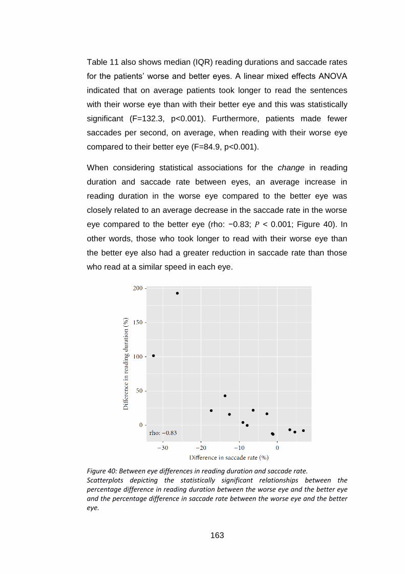
163
Table 11 also shows median (IQR) reading durations and saccade rates
for the patients’ worse and better eyes. A linear mixed effects ANOVA
indicated that on average patients took longer to read the sentences
with their worse eye than with their better eye and this was statistically
significant (F=132.3, p<0.001). Furthermore, patients made fewer
saccades per second, on average, when reading with their worse eye
compared to their better eye (F=84.9, p<0.001).
When considering statistical associations for the change in reading
duration and saccade rate between eyes, an average increase in
reading duration in the worse eye compared to the better eye was
closely related to an average decrease in the saccade rate in the worse
eye compared to the better eye (rho: −0.83; < 0.001; Figure 40). In
other words, those who took longer to read with their worse eye than
the better eye also had a greater reduction in saccade rate than those
who read at a similar speed in each eye.
Figure 40: Between eye differences in reading duration and saccade rate. Scatterplots depicting the statistically significant relationships between the percentage difference in reading duration between the worse eye and the better eye and the percentage difference in saccade rate between the worse eye and the better eye.

164
Associations in differences in visual function measures between the
better and worse eye compared with reading duration and saccade rate
are shown in Table 12.
Table 12: Spearman’s rho correlations comparing the difference in reading duration between the worse eye and the better eye and the difference in saccade rate between the worse eye and the better eye, with key measured variables relating to age and vision.
Difference between eyes
24-2 MD 10-2 MD
Mean
central
VF points
CS VA Age
Change in reading
duration per trial rho
(P-value)
-0.20
(0.48)
0.13
(0.65)
0.01
(0.99)
-0.41
(0.14)
0.35
(0.14)
0.17
(0.56)
Change in Saccade
rate rho (P-value)
0.19
(0.51)
-0.32
(0.26)
0.21
(0.47)
0.65*
(0.01)
-0.56*
(0.04)
-0.09
(0.76)
Figure 41: Relationship of between eye differences in saccade rate with differences in contrast sensitivity and visual acuity. Scatterplots depicting the statistically significant relationships between (left) the difference in contrast sensitivity (log) and percentage difference in saccade rate between eyes, and (right) the difference in logMAR visual acuity and the percentage difference in saccade rate between eyes.

165
There was noteworthy association between changes in saccade rate
and the extent of difference in contrast sensitivity between the better
and worse eye. So those with a greater reduction in contrast sensitivity
in the worse eye were more likely to have a reduced saccade rate in the
worse eye (Figure 41 (left)). Furthermore, those patients with a greater
drop in visual acuity in their worse eye also showed a greater reduction
in saccade rate (Figure 41 (right)). There were no other statistically
significant correlations (Table 12).
Table 13 shows the proportion of saccades classified as each of the
four eye movement types for the better and worse eyes, respectively.
There were no statistically significant differences in these values
between eyes. However, a larger increase in reading duration in the
worse eye compared to the better eye was associated with an increase
in the percentage of eye movements that were regressions in the worse
eye compared to the better eye (rho: 0.60; < 0.03; Figure 42 (left)). In
addition, a greater increase in reading duration in the worse eye
compared to the better eye was associated with making more unknown
eye movements in the worse eye compared to the better eye (rho: 0.59;
< 0.03; Figure 42 (right)).
Table 13: Proportion of saccades that were forward, between lines, regressions or unknown when reading with the best eye and worse eye, respectively.
Better eye Worse eye
Between word (%, median, IQR) 72.0 (70.1, 73.5) 67.2 (62.4, 75.1)
Line change (%, median, IQR) 10.6 (9.0, 11.3) 10.2 (9.0, 11.1)
Regressions (%, median, IQR) 11.4 (9.7, 15.4) 13.8 (10.9, 19.7)
Unknown (%, median, IQR) 5.6 (3.7, 8.4) 6.5 (4.2, 9.8)
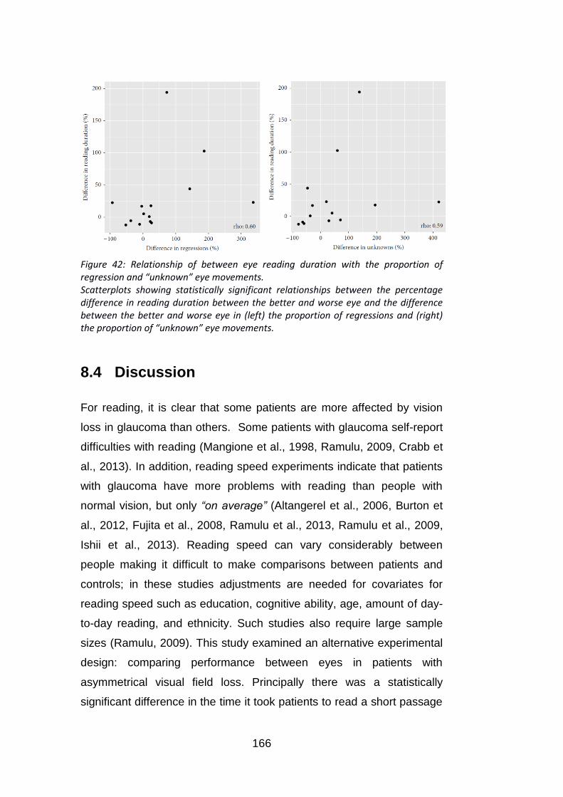
166
Figure 42: Relationship of between eye reading duration with the proportion of regression and “unknown” eye movements. Scatterplots showing statistically significant relationships between the percentage difference in reading duration between the better and worse eye and the difference between the better and worse eye in (left) the proportion of regressions and (right) the proportion of “unknown” eye movements.
8.4 Discussion
For reading, it is clear that some patients are more affected by vision
loss in glaucoma than others. Some patients with glaucoma self-report
difficulties with reading (Mangione et al., 1998, Ramulu, 2009, Crabb et
al., 2013). In addition, reading speed experiments indicate that patients
with glaucoma have more problems with reading than people with
normal vision, but only “on average” (Altangerel et al., 2006, Burton et
al., 2012, Fujita et al., 2008, Ramulu et al., 2013, Ramulu et al., 2009,
Ishii et al., 2013). Reading speed can vary considerably between
people making it difficult to make comparisons between patients and
controls; in these studies adjustments are needed for covariates for
reading speed such as education, cognitive ability, age, amount of day-
to-day reading, and ethnicity. Such studies also require large sample
sizes (Ramulu, 2009). This study examined an alternative experimental
design: comparing performance between eyes in patients with
asymmetrical visual field loss. Principally there was a statistically
significant difference in the time it took patients to read a short passage
167
of text in what is considered to be their worse eye (most visual field
damage) when compared to their better eye (least visual field damage).
This was done in a small sample of patients that carried out the reading
task many times. The effect size was, however, small and the difference
in reading duration between eyes was not associated with the
magnitude of the difference between visual field loss between the two
tested eyes. In other words there was no “dose” effect: larger
differences in severity of visual field defect between eyes were not
associated with worse performance. This was true for the MD from a
standard clinical visual field test (24-2 HFA) and a visual field test of
more central areas (10-2 HFA). It is therefore unclear if an overall
summary measure of visual field defect severity can be predictive of
worsening reading performance in glaucoma. There was no significant
difference between eyes for visual acuity when considering the average
of all patients; this finding likely reflects the fact that many patients with
worsening glaucoma maintain relatively good visual acuity while other
aspects of visual function decline. However, when considering within-
person differences in visual acuity in the worse versus the better eye, a
larger decline in visual acuity was associated with a greater reduction in
reading speed in the worse eye. This finding highlights the benefits of
considering performance changes within each individual in addition to
considering average effects across all participants. The magnitude of
the difference in contrast sensitivity between eyes was also related to
difference in reading performance between eyes. The important role of
contrast sensitivity in reading performance in glaucoma has been
emphasised elsewhere (Burton et al., 2012).
This experiment was novel in comparison with most other studies
investigating reading performance in people with glaucoma because it
took advantage of measurements from an eye tracker. Patients had a
reduced saccade rate (making fewer saccades per second) on average
when reading with their worse eye compared to their better eye.
Furthermore, average saccade rate was strongly associated with

168
reading duration. These findings imply that saccade rate, measured by
an eye tracker, could be a useful surrogate for reading performance. A
reduction in saccade rate in patients with visual field defects has also
been observed in other studies involving different visual tasks (Smith et
al., 2012b, Smith et al., 2012a) and other experimental results suggest
that saccadic initiation in patients with glaucoma is delayed relative to
controls with healthy vision (Kanjee et al., 2012). It may be that visual
function loss caused by glaucoma impairs the ability of the visual
system to process the surrounding information during each glance,
meaning that it takes longer to initiate a saccade towards relevant
information. Nevertheless, although reduced reading duration and
saccade rate were observed on average for the worse eye compared to
the better eye, the degree of change between eyes varied considerably
across patients. For example, Figure 40 showed that certain patients
had a much longer reading duration for the worse eye and also tended
to show a more reduced saccade rate. However, other patients
appeared to be less affected in terms of reading speed when reading
with their worse eye and these people also tended to maintain a similar,
or increased, saccade rate to the better eye.
Typically when reading, there will be a window of information that can
be absorbed during each fixation, referred to as the “perceptual span”.
Visual degradation caused by visual field defects can be expected to
reduce the number of characters that can be read with each fixation
(Loftus et al., 1992) (Bullimore and Bailey, 1995), suggesting that more
saccades must subsequently be made in order to process the same
quantity of information. Therefore, some patients may have maintained
an adequate reading speed when reading with their worse eye by
increasing their saccadic rate in order to overcome the impairment that
would normally be expected due to the visual degradation. This result
coincides, in part, with a finding that suggests glaucomatous visual field
loss restricts saccades during other tasks such as visual search, but
that increasing saccade rate is associated with maintaining good
169
performance (Smith et al., 2012b). It is unknown whether these eye
movements are adaptive behaviour, thus it would be worthwhile to
study this topic in future investigations.
Eye-tracking generates copious data that can be easily misidentified or
misinterpreted. Eye movement analysis software for reading
experiments typically provides scanpath data (Kabanarou and Rubin,
2006, Crossland and Rubin, 2006, Rubin and Feely, 2009) that has to
be manually delineated to extract specific saccades like regressions (a
backtracking saccade sometimes observed during reading). In this
study automated techniques were developed for identifying the different
types of eye movements made during the reading task. In this
experiment, there was no statistically significant difference in the types
of eye movements identified by the algorithm made by the eye with
more visual field damage compared to the eye with less visual field
damage. Still, there was a relationship between increases in the
proportion of regressions and worse reading performance. The
algorithm also automatically identified unknown or “irregular” eye
movements that were associated with poorer reading performance in
the worse eye compared to the better eye. Patients who followed more
conventional reading patterns (making a smaller proportion of
regressions and unknown eye movements compared to ‘forward’
saccades between words) in both eyes appeared to read equally
quickly in both eyes. These findings illustrate the utility of eye tracking in
studies of reading in glaucoma and hint at the design of future studies.
For example, recent research suggests that reading performance in
patients with glaucoma is particularly affected during sustained reading
as opposed to when reading short passages of text (Ramulu et al.,
2013); it might be useful to use eye tracking in future experiments of
that type.
There are limitations associated with our study. There was no
assessment of comprehension of the texts and the nature of the reading
170
experiment – large font size and reading from a computer screen –
does not mimic everyday reading. The sample size was not large
enough to tease out any statistically significant differences in the types
of eye movements that might be used by an eye with worse visual field
damage compared to one with less visual field damage. The small
sample size also did not allow to explore how reading performance is
affected by the precise location of a visual field defect or how a similar
visual field defect in the right eye as compared to the left eye might
influence performance; this awaits further study. Future research may
also wish to consider the performance of people with asymmetric visual
field loss when reading bilaterally and whether this is comparable to
reading monocularly with the better or worse eye. It is also important to
point out that the methods for preprocessing the eye movement data
and for automatically classifying their properties have not been
validated or compared with manual methods. Nevertheless, the study
still adds to the literature by showing the potential of eye tracking for
understanding how patients with visual field defects function in
everyday tasks such as reading.
In summary, this study has shown that patients with glaucoma will take
longer to read a short passage of text in what is considered to be their
worse eye (most visual field damage) when compared to their better
eye (least visual field damage). However, the effects were small.
Unexpectedly, reading performance did not worsen in the eye with most
visual field damage as the between-eye differences in visual field defect
severity increased (as measured by a single summary measure of the
visual field). The novel analytical eye movement data analysis
presented in this chapter might be useful for other reading studies. The
results suggest that regressions and unknown saccades result in slower
reading speeds. In conclusion, this novel experimental design might
help unravel the relationship between glaucomatous vision loss and
difficulties with reading. For example, a future study comparing
performance between eyes and using eye tracking could help
171
determine the precise location of visual field loss that inhibits reading
performance in glaucoma.

172
9. Conclusions and Future Research
The establishment of static automated perimetry as the gold standard
visual field examination in patients with glaucoma brought many
advantages: an easy operation of the test, efficient test procedures,
examiner independent measures, the evaluation of age-related
normative ranges of contrast sensitivity in the visual field and
standardised analyses of the results. However, it also led to a focus on
the central 30˚. Yet, the information that is lost regarding the peripheral
visual field might be of value. It could help to understand how patients
are affected in their everyday life and which disabilities might go along
with their individual visual field loss. It could increase the dynamic range
for monitoring progression of disease or in some cases might even help
detection.
The aim of this thesis was to lay groundwork for the development of a
fully automated test of the peripheral visual field.
9.1 Key findings
9.1.1 Automated kinetic perimetry in the peripheral visual
field
The examination of a peripheral isopter was found to provide additional
information about the overall visual field loss in patients with glaucoma.
The automated estimation of isopters was repeatable. The repeatability
of the kinetic test was similar to the repeatability of a static automated
test (GATE, 24-2) of the central visual field (see Chapter 5, page 83 ff).
I demonstrated that data-driven simulations can be a useful tool to
evaluate the efficiency of kinetic procedures. I showed that the

173
response behaviour did not follow a Gaussian distribution. Instead, the
distribution of responses was steep and positively skewed with long,
narrow tails indicating that most responses are closely located around
isopter locations with occasional responses in further distances. These
distances tended to be larger outside than inside the isopter. To
estimate isopters with good accuracy and precision, repeated
presentations were found to be essential. A large gain in precision was
achieved by using at least three responses per meridian to estimate the
isopter. The use of adaptive rules was shown to reduce the required
number of stimuli, while still achieving comparably high accuracy and
precision (see Chapter 6, page 103 ff).
9.1.2 Threshold estimation with static stimuli in the
peripheral visual field
Size V stimuli were found to be more suitable for threshold estimation
with static stimuli in the peripheral visual field than size III stimuli, as
they yielded higher contrast sensitivity and lower response variability.
The overall relation between response variability and contrast sensitivity
was in line with previous studies (Henson et al., 2000, Russell et al.,
2012a). Predictably, estimates with high contrast sensitivity were more
reliable than those with low contrast sensitivity. However, there was a
trend for response variability with respect to contrast sensitivity to be
slightly lower in the peripheral (beyond 30˚) than in the central visual
field (≤30˚). Thus static threshold estimation in the peripheral visual field
might be more reliable than predicted by a previous model between
response variability and contrast sensitivity (Henson et al., 2000).
I found contrast sensitivity to be lower for static than for kinetic III1e
stimuli. In accordance with a previous study, which examined the
dissociation of static and kinetic contrast sensitivity for a range of other
stimulus parameters, this difference was on average about 5 dB
(Hudson and Wild, 1992) (see Chapter 7, page 121 ff). There was large

174
variability in the difference between static and kinetic contrast
sensitivity. The cause of this variability is still unknown.
9.1.3 Reading performance in patients with glaucoma
I demonstrated that an intra-patient between-eye design in glaucoma
patients with greater visual field loss in one eye than the other permits
the investigation of the relationship between disability and visual field
loss even in small samples. There was a significant decrease in reading
performance when reading with the eye with greater visual field loss
compared to reading with the better eye. Worse reading performance
was found to be related to changes in eye movement patterns. A lower
reading speed was associated with a decreased rate of saccades in the
worse eye. A decrease in reading speed in the worse eye was also
associated with a relative increase in regressions (saccades that
backtrack to previous parts of text) (see Chapter 8, page 150 ff).
9.2 Implications of findings and future research
9.2.1 Development of a fully automated test strategy for
the peripheral visual field
9.2.1.1 Kinetic perimetry in the peripheral visual field
As part of this thesis, I designed an automated kinetic test that
examines a peripheral isopter with three repeated stimuli along each
meridian. I suggested the mean isopter radius as a summary measure,
as it provides a more intuitive idea of the size of the isopter than the
often used isopter area without compromising information. As several
responses were sampled per meridian in each test, I introduced an
estimate of response variability within single tests (median absolute
deviation of single responses) that can be used as an indicator of test

175
variability. I showed that isopters could be estimated with good
repeatability with this test. A data-driven simulation of responses to
kinetic stimuli revealed that at least three responses are required to
estimate isopters with good precision and accuracy.
However, tests with three repeated presentations per meridian are of
too long duration for a clinical application. Automated kinetic perimetry
with adaptive procedures has previously been suggested (Hashimoto et
al., 2015, Johnson et al., 1987). I therefore asked whether adaptive
rules could deliver a comparable information gain at smaller costs of
testing time. Indeed I found that such rules permit the estimation of
isopters more efficiently, while not compromising on accuracy or
precision. Using a computer simulation, I evaluated a simple adaptive
rule in which the presentation of a third stimulus per isopter depends on
the distance between the two previous responses. With this rule
isopters could be estimated with equal precision and accuracy as
provided by a test with three repetitions per isopter while reducing the
required stimulus number by about 25%.
A rule that is used in both Johnson’s strategy and Matsumoto et al.’s
Program K is that if responses occur within a normal range, the first
response is accepted as the isopter location (Hashimoto et al., 2015,
Johnson et al., 1987). Computer simulations, as performed in Chapter
6, could be used to estimate how likely it is that responses occur within
a normal range when the true isopter location is actually abnormal. To
establish automated kinetic tests as a standard test for the examination
of peripheral visual fields, the efficiency of test procedures needs to be
optimised. I propose to use simulations to evaluate the efficiency of
different strategies, as it permits the comparison of the performance of
many different versions of test procedures in a short amount of time.
Notably, in this thesis, I investigate responses to kinetic stimuli with only
one stimulus type (Goldmann III1e moved at 5˚/sec). However response
variability might vary depending on stimulus parameters (size, contrast,

176
speed). In Chapter 6 I found that response variability was independent
of eccentricity for III1e stimuli and speculated that it could be indicative
of a constant relationship between contrast sensitivity and response
variability as similarly found for static stimuli. Understanding the relation
between different stimulus parameters and response variability would
help to formulate models for response behaviour in kinetic perimetry.
Moreover, investigating the relationship between stimulus size and
response variability could help to determine what the most suitable
stimulus size is for kinetic perimetry of the peripheral visual field. For
example, in static perimetry, size V (diameter: 1.72˚) stimuli appear to
be more suitable in the far periphery. The kinetic automated test to
measure a peripheral isopter with repeated presentations introduced in
this thesis uses Goldmann size III stimuli (diameter: 0.43˚).
Traditionally, in Goldmann perimetry the smallest stimuli (size I,
diameter: 0.11˚) are used to examine the entire visual field and larger
sizes are only introduced when advanced visual field loss is present
and an increase of stimulus intensity through an increase in contrast is
not sufficient.
9.2.1.2 Threshold estimation with static stimuli in the
peripheral visual field
In Chapter 7 I investigated threshold estimation with static stimuli in the
peripheral visual field. Size V stimuli were shown to be most suitable for
static perimetry in the peripheral visual field as compared to size III
stimuli: Contrast sensitivity was higher and response variability lower
when measuring with size V stimuli in the peripheral visual field. Thus
they provide a larger dynamic range in which the visual field can be
measured reliably. My findings agreed with previous findings evaluating
the influence of stimulus size on contrast sensitivity and response
variability (Redmond et al., 2010, Fellman et al., 1988, Dannheim and
Drance, 1971, Wilson, 1970, Wald, 1938, Gardiner et al., 2013, Wall et

177
al., 2013, Wall et al., 1997) and corroborate the theory that response
variability and contrast sensitivity depend on the number of ganglion
cells that respond to a specific stimulus (Wilson, 1970, Swanson et al.,
2004, Fischer, 1973, Anderson, 2006). Since ganglion cell density is
lower in the peripheral visual field than in the central visual field, the
stimulus area needs to be increased in the peripheral field to activate
the same number of ganglion cells and thus to result in equivalent
contrast sensitivity. This is equally true in areas of visual field loss.
Crucially, this kind of spatial summation of the signal is thought to be
constant up to a certain area in the visual field in which is covered by
the receptive fields of a specific number of ganglion cells (Ricco’s area)
(see Chapter 2.1.4.2.1, page 44). When exceeding this area the
additional gain in signal decreases. Crucially, these properties predict
that increasing the stimulus area would lead to a larger gain in contrast
sensitivity in areas with lower ganglion cell density. In line with this
biologically inspired prediction, I found a smaller difference in contrast
sensitivity to size III and V stimuli in the central than the peripheral
visual field. But a similar increase in contrast sensitivity throughout the
visual field in patients with glaucoma. Therefore the optimal stimulus
size to achieve a good dynamic range without losing the power to
detect abnormal contrast sensitivities might be to match the stimulus
size to the size of Ricco’s area in the respective location of a normal
visual field.
On average, I found a similar relation between response variability and
contrast sensitivity for size III stimuli as in previous studies. However,
by tendency, the ratio of response variability over contrast sensitivity
was smaller in peripheral than central locations. To my best knowledge,
this has not been shown to date. If this difference in the relation
between contrast sensitivity and response variability in the periphery
holds true it implies that static threshold estimation is more reliable in
the periphery than expected. It also indicates that reduced central
ganglion cell density related to disease has a different effect on

178
response variability than physiologically low ganglion cell density in the
peripheral visual field. Further research here could lead to important
findings to conclusively study the relationship between response
variability and contrast sensitivity in the peripheral visual field.
9.2.1.3 Combined static kinetic automated perimetry
My findings in Chapter 7 indicated that results between kinetic and
static stimuli are different. On average, a simple constant could be
added to translate kinetic and static stimuli into the same reference
frame. However, the difference between kinetic and static contrast
sensitivity is strongly variable and the cause for this variability is still
unknown. Here, I only examined the relation for one stimulus type
(III1e), but a previous study found similar average differences for a
range of stimulus contrasts and sizes I and III.
A combined kinetic and static test might be an efficient way to examine
the entire visual field. Here, an isopter could be estimated first and
establish a region of interest within which thresholds are estimated with
static perimetry. The estimated isopter could provide prior information
about expected contrast sensitivities at nearby locations. This
information could be integrated as a prior into combined static kinetic
procedures to increase the efficiency of threshold estimation at such
locations. Moreover, such a test would eliminate static test locations in
regions with low contrast sensitivity near 0 dB. Static thresholds
estimated in such regions have high variability and thus do not provide
reliable information. Furthermore, in many procedures more stimuli are
required to estimate contrast sensitivities in regions with highly
abnormal contrast sensitivities. Thus time consuming threshold
estimation in regions of the peripheral visual field that do not provide
much information could be prevented by estimating a peripheral isopter
first. Further work might lead to a test that could save time when
examining the visual field in patients with advanced glaucomatous
damage.

179
9.2.2 Functional relevance of measuring the peripheral
visual field
9.2.2.1 Does an examination of the peripheral visual field
beyond 30˚ add information?
An examination beyond 30˚ in patients with glaucoma is only useful if it
adds valuable information. This could be clinically useful information for
glaucoma diagnosis or monitoring of disease progression. It may also
be relevant information about how an individual is affected by his or her
visual field loss. Simply put, if peripheral visual field loss cannot be
predicted based on information from the central visual field, then this
space might be clinically useful.
Indeed, I found that measuring the peripheral visual field added
information to results of static tests of the central visual field. There was
only a loose relationship between central and peripheral field loss and
the extent of peripheral loss could vary widely in patients with a similar
extent of central loss. Several patients with advanced central visual field
loss were found to have preserved areas in the peripheral visual field.
The examination of such preserved peripheral areas in addition to the
central visual field can improve the monitoring of disease progression in
advanced glaucoma (Nowomiejska et al., 2014). In the study presented
in Chapter 5 patients with various stages of central visual field loss were
recruited. In the range of patients with moderate to advanced central
visual field loss, central and peripheral visual field damage was loosely
related. Only one of the glaucoma patients in this study had little or no
central visual field loss. The specific recruitment of a group of patients
with no or low central visual field loss (e.g. patients with ocular
hypertension) would be useful to further investigate the relation
between central and peripheral visual field loss in early glaucoma.
Previous studies examining such groups found peripheral visual field

180
damage in the absence of central visual field loss in 7% and 4% of
patients respectively (Miller et al., 1989, Ballon et al., 1992).
The aim in this study was to investigate the relationship between central
and peripheral visual field damage based on commonly used summary
measures indicating the overall extent of visual field loss. An interesting
question that went beyond the scope of this thesis would be how the
exact patterns of central and peripheral visual field loss are related. A
detailed shape analysis of isopters and the topography of the central
visual field would be required to examine this topic further.
9.2.2.1 Which functional abilities are related to peripheral
vision?
I found that investigating the peripheral visual field adds information to
central visual field results. The question remains how peripheral visual
field loss affects a patient. Peripheral vision might be especially
essential when it comes to mobility. Peripheral vision has been shown
to contribute to postural control, which in turn when impaired can
increase the risk for falls. In Chapter 5 I found a relationship between
both, central (≤30˚) and peripheral (>30˚) visual field loss and self
reported fear of falling. However, the confidence intervals of the
correlation coefficients varied substantially. Larger sample sizes of at
least 100 participants would be needed to conclusively study this
relationship. In Chapter 8, in a departure from the central themes of the
thesis, I demonstrated that a between-eye, intra-subject design in
patients with greater visual field loss in one eye than the other is a
promising way to investigate the relationship between visual field loss
and reading performance even in small samples. Such a design could
also be utilised to examine the relationship between peripheral visual
field loss and other functional abilities such as postural control.
However, not just balance, but also other mechanisms that indirectly
influence mobility could be disturbed through peripheral visual field loss.

181
Peripheral vision is, for example, important to guide attention to salient
stimuli in the visual field. An orientation towards a salient stimulus in
extra-foveal regions occurs in an involuntary reflexive manner (Muller
and Rabbitt, 1989). The failure to detect such cues in the peripheral
visual field could lead to an increased risk for accidents. Indeed,
simulated visual field defects have been shown to significantly impair
hazard detection (Glen et al., 2014). Moreover, glaucoma was found to
be connected to a higher risk for car accidents (Haymes et al., 2007).
An investigation of the relation between visual field damage and the
guidance of attention to salient cues in different eccentricities in the
visual field could help to understand which decrease in contrast
sensitivity in specific locations of the visual field leads to a disturbance
of involuntary attention orienting mechanisms.
Peripheral vision has also been shown to be involved in differentiating
between egocentric versus exocentric motion in the absence of
vestibular input (Brandt et al., 1973). When stimuli could only be
perceived in the central 30˚ optokinetic stimuli were perceived as the
environment appearing to move, while optokinetic stimuli presented in
the entire or peripheral visual field led to a perception of self-motion.
The judgement of the velocity of self-motion matched the velocity of
optokinetic stimuli. When looking in the direction of our path of motion,
optic flow allows us to estimate motion speed. Optic flow is stronger the
further away visual input is from fixation, meaning that the effect of optic
flow is higher in the visual field periphery than in the central visual field.
Thus the judgement of self-motion and estimation of velocity might be
affected by peripheral visual field loss.
Vision loss in the periphery might have detrimental effects on functional
abilities, especially affecting mobility in various ways (disturbed postural
control, hazard detection and motion perception). Thus, a closer
examination of visual disabilities in patients with glaucoma and
peripheral visual field loss is needed. The availability of an efficient

182
automated standard examination of the peripheral visual field would
help such studies and would increase comparability between studies.
The findings in this thesis are an important step towards the
development of an efficient automated test for the peripheral visual
field.

183
References
ALTANGEREL, U., SPAETH, G. L. & STEINMANN, W. C. 2006. Assessment of Function Related to Vision (AFREV). Ophthalmic Epidemiology, 13, 67 - 80.
AMBLARD, B. & CARBLANC, A. 1980. Role of foveal and peripheral visual information in maintenance of postural equilibrium in man. Perceptual and Motor Skills, 51, 903-912.
ANAND, V., BUCKLEY, J. G., SCALLY, A. & ELLIOTT, D. B. 2003. Postural stability changes in the elderly with cataract simulation and refractive blur. Invest Ophthalmol Vis Sci, 44, 4670-5.
ANDERSON, D. R. 1987. Perimetry, With and Without Automation. Wiley Online Library.
ANDERSON, R. S. 1996. The selective effect of optical defocus on detection and resolution acuity in peripheral vision. Current eye research, 15, 351-353.
ANDERSON, R. S. 2006. The psychophysics of glaucoma: improving the structure/function relationship. Prog Retin Eye Res, 25, 79-97.
ARFKEN, C. L., LACH, H. W., BIRGE, S. J. & MILLER, J. P. 1994. The prevalence and correlates of fear of falling in elderly persons living in the community. Am J Public Health, 84, 565-70.
ARMALY, M. F. 1971. Visual field defects in early open angle glaucoma. Trans Am Ophthalmol Soc, 69, 147-62.
ARTES, P. H., HUTCHISON, D. M., NICOLELA, M. T., LEBLANC, R. P. & CHAUHAN, B. C. 2005. Threshold and variability properties of matrix frequency-doubling technology and standard automated perimetry in glaucoma. Invest Ophthalmol Vis Sci, 46, 2451-7.
ARTES, P. H., IWASE, A., OHNO, Y., KITAZAWA, Y. & CHAUHAN, B. C. 2002. Properties of perimetric threshold estimates from Full Threshold, SITA Standard, and SITA Fast strategies. Invest Ophthalmol Vis Sci, 43, 2654-9.
ARTES, P. H., O'LEARY, N., HUTCHISON, D. M., HECKLER, L., SHARPE, G. P., NICOLELA, M. T. & CHAUHAN, B. C. 2011. Properties of the Statpac Visual Field Index. Investigative Ophthalmology & Visual Science, 52, 4030-4038.
ASAOKA, R., CRABB, D. P., YAMASHITA, T., RUSSELL, R. A., WANG, Y. X. & GARWAY-HEATH, D. F. 2011. Patients have two eyes!: binocular versus better eye visual field indices. Investigative ophthalmology & visual science, 52, 7007-7011.
ÅSMAN, P. & HEIJL, A. 1992. Glaucoma hemifield test: automated visual field evaluation. Archives of ophthalmology, 110, 812-819.
ASPINALL, P. A., JOHNSON, Z. K., AZUARA-BLANCO, A., MONTARZINO, A., BRICE, R. & VICKERS, A. 2008. Evaluation of quality of life and priorities of patients with glaucoma. Invest Ophthalmol Vis Sci, 49, 1907-15.
ASSAIANTE, C. & AMBLARD, B. 1992. Peripheral vision and age-related differences in dynamic balance. Human Movement Science, 11, 533-548.
BAEZ, K. A., MCNAUGHT, A. I., DOWLER, J. G., POINOOSAWMY, D., FITZKE, F. W. & HITCHINGS, R. A. 1995. Motion detection threshold and field progression in normal tension glaucoma. Br J Ophthalmol, 79, 125-8.
184
BALLON, B. J., ECHELMAN, D. A., SHIELDS, M. B. & OLLIE, A. R. 1992. Peripheral visual field testing in glaucoma by automated kinetic perimetry with the Humphrey Field Analyzer. Arch Ophthalmol, 110, 1730-2.
BARDY, B. G., WARREN, W. H., JR. & KAY, B. A. 1999. The role of central and peripheral vision in postural control during walking. Percept Psychophys, 61, 1356-68.
BATHIJA, R., GUPTA, N., ZANGWILL, L. & WEINREB, R. N. 1998. Changing definition of glaucoma. J Glaucoma, 7, 165-9.
BEBIE, H., FANKHAUSER, F. & SPAHR, J. 1976. Static perimetry: strategies. Acta Ophthalmol (Copenh), 54, 325-38.
BENGTSSON, B. & HEIJL, A. 1998a. Evaluation of a new perimetric threshold strategy, SITA, in patients with manifest and suspect glaucoma. Acta Ophthalmol Scand, 76, 268-72.
BENGTSSON, B. & HEIJL, A. 1998b. SITA Fast, a new rapid perimetric threshold test. Description of methods and evaluation in patients with manifest and suspect glaucoma. Acta Ophthalmol Scand, 76, 431-7.
BENGTSSON, B. & HEIJL, A. 1999. Inter-subject variability and normal limits of the SITA Standard, SITA Fast, and the Humphrey Full Threshold computerized perimetry strategies, SITA STATPAC. Acta Ophthalmol Scand, 77, 125-9.
BENGTSSON, B., HEIJL, A. & OLSSON, J. 1998. Evaluation of a new threshold visual field strategy, SITA, in normal subjects. Swedish Interactive Thresholding Algorithm. Acta Ophthalmol Scand, 76, 165-9.
BENGTSSON, B., OLSSON, J., HEIJL, A. & ROOTZEN, H. 1997. A new generation of algorithms for computerized threshold perimetry, SITA. Acta Ophthalmol Scand, 75, 368-75.
BERENCSI, A., ISHIHARA, M. & IMANAKA, K. 2005. The functional role of central and peripheral vision in the control of posture. Hum Mov Sci, 24, 689-709.
BERENS, C. 1923. Examination of the Blind Spot of Mariotte. Trans Am Ophthalmol Soc, 21, 271-90.
BERENS, P. 2009. CircStat: a MATLAB toolbox for circular statistics. J Stat Softw, 31, 1-21.
BEREZINA, T. L., KHOURI, A. S., KOLOMEYER, A. M., CLANCY, P. S. & FECHTNER, R. D. 2011. Peripheral visual field thresholds using Humphrey Field Analyzer program 60-4 in normal eyes. Eur J Ophthalmol, 21, 415-21.
BEREZINA, T. L., KHOURI, A. S., WINSHIP, M. D. & FECHTNER, R. D. 2012. Visual field and ocular safety during short-term vigabatrin treatment in cocaine abusers. Am J Ophthalmol, 154, 326-332 e2.
BITTNER, A. K., IFTIKHAR, M. H. & DAGNELIE, G. 2011. Test-retest, within-visit variability of Goldmann visual fields in retinitis pigmentosa. Invest Ophthalmol Vis Sci, 52, 8042-6.
BJERRE, A., CODINA, C. & GRIFFITH, H. 2014. Peripheral Visual Fields in Children and Young Adults Using Semi-automated Kinetic Perimetry: Feasibility of Testing, Normative Data, and Repeatability. Neuro-Ophthalmology, Early Online, , 1744-506X online 1–10.
BLACK, A. A., WOOD, J. M. & LOVIE-KITCHIN, J. E. 2011. Inferior field loss increases rate of falls in older adults with glaucoma. Optom Vis Sci, 88, 1275-82.
BLAND, J. M. & ALTMAN, D. G. 1986. Statistical methods for assessing agreement between two methods of clinical measurement. Lancet, 1, 307-10.
BLOCH, A. 1885. Experiences sur la vision. CR Seances Soc. Biol. Paris, 37, 493-495.

185
BOWERS, A., PELI, E., ELGIN, J., MCGWIN, G., JR. & OWSLEY, C. 2005. On-road driving with moderate visual field loss. Optom Vis Sci, 82, 657-67.
BRANDT, T., DICHGANS, J. & KOENIG, E. 1973. Differential effects of central verses peripheral vision on egocentric and exocentric motion perception. Exp Brain Res, 16, 476-91.
BRENTON, R. S. & PHELPS, C. D. 1986. The normal visual field on the Humphrey field analyzer. Ophthalmologica, 193, 56-74.
BRINDLEY, G. 1952. The Bunsen‐Roscoe law for the human eye at very short durations. The Journal of physiology, 118, 135-139.
BROADWAY, D. C. 2012. Visual field testing for glaucoma - a practical guide. Community Eye Health, 25, 66-70.
BROMAN, A. T., QUIGLEY, H. A., WEST, S. K., KATZ, J., MUNOZ, B., BANDEEN-ROCHE, K., TIELSCH, J. M., FRIEDMAN, D. S., CROWSTON, J., TAYLOR, H. R., VARMA, R., LESKE, M. C., BENGTSSON, B., HEIJL, A., HE, M. & FOSTER, P. J. 2008. Estimating the rate of progressive visual field damage in those with open-angle glaucoma, from cross-sectional data. Invest Ophthalmol Vis Sci, 49, 66-76.
BRUSINI, P. 1997. A comparison of three methods for distinguishing between diffuse, localized and mixed visual field defects in glaucoma. Perimetry update 1996/1997. Kulger Amsterdam/New York.
BULLIMORE, M. A. & BAILEY, I. L. 1995. Reading and Eye Movements in Age-Related Maculopathy. Optometry & Vision Science, 72, 125-138.
BURR, J. M., KILONZO, M., VALE, L. & RYAN, M. 2007. Developing a preference-based Glaucoma Utility Index using a discrete choice experiment. Optom Vis Sci, 84, 797-808.
BURTON, H., SNYDER, A. Z., CONTURO, T. E., AKBUDAK, E., OLLINGER, J. M. & RAICHLE, M. E. 2002. Adaptive changes in early and late blind: a fMRI study of Braille reading. J Neurophysiol, 87, 589-607.
BURTON, R., CRABB, D. P., SMITH, N. D., GLEN, F. C. & GARWAY-HEATH, D. F. 2012. Glaucoma and reading: exploring the effects of contrast lowering of text. Optom Vis Sci., 89, 1282-7. doi: 10.1097/OPX.0b013e3182686165.
BURTON, R., SAUNDERS, L. J. & CRABB, D. P. 2015. Areas of the visual field important during reading in patients with glaucoma. Jpn J Ophthalmol, 59, 94-102.
BURTON, R., SMITH, N. D. & CRABB, D. P. 2014. Eye movements and reading in glaucoma: observations on patients with advanced visual field loss. Graefes Arch Clin Exp Ophthalmol, 252, 1621-30.
CALIXTO, N., SANTOS, R. M. D. O. & CRONEMBERGER, S. 2006. Visual field (Octopus 1-2-3) in normal subjects divided into homogeneous age-groups. Arquivos brasileiros de oftalmologia, 69, 637-643.
CAMPBELL, A. J., BORRIE, M. J. & SPEARS, G. F. 1989. Risk factors for falls in a community-based prospective study of people 70 years and older. J Gerontol, 44, M112-7.
CAPRIOLI, J. & SPAETH, G. L. 1985. Static threshold examination of the peripheral nasal visual field in glaucoma. Arch Ophthalmol, 103, 1150-4.
CASSON, E. J., OSAKO, M., JOHNSON, C. A. & HWANG, P. 1991. Temporal and spatial response properties of optic neuritis patients manifesting statokinetic dissociation. Appl Opt, 30, 2136-42.
CASSON, R. J., CHIDLOW, G., WOOD, J. P., CROWSTON, J. G. & GOLDBERG, I. 2012. Definition of glaucoma: clinical and experimental concepts. Clin Experiment Ophthalmol, 40, 341-9.

186
CERULLI, A., CESAREO, M., CIUFFOLETTI, E., MONTANARO, M. L., MANCINO, R., MIRISOLA, C., SORGE, R., CEDRONE, C., NUCCI, C. & CERULLI, L. 2014. Evaluation of eye movements pattern during reading process in patients with glaucoma: a microperimeter study. Eur J Ophthalmol, 24, 358-63.
CHAUHAN, B. C., TOMPKINS, J. D., LEBLANC, R. P. & MCCORMICK, T. A. 1993. Characteristics of frequency-of-seeing curves in normal subjects, patients with suspected glaucoma, and patients with glaucoma. Invest Ophthalmol Vis Sci, 34, 3534-40.
CHRISTOFORIDIS, J. B. 2011. Volume of visual field assessed with kinetic perimetry and its application to static perimetry. Clin Ophthalmol, 5, 535-41.
COLEMAN, A. L., CUMMINGS, S. R., ENSRUD, K. E., YU, F., GUTIERREZ, P., STONE, K. L., CAULEY, J. A., PEDULA, K. L., HOCHBERG, M. C. & MANGIONE, C. M. 2009. Visual field loss and risk of fractures in older women. J Am Geriatr Soc, 57, 1825-32.
COLEMAN, A. L., CUMMINGS, S. R., YU, F., KODJEBACHEVA, G., ENSRUD, K. E., GUTIERREZ, P., STONE, K. L., CAULEY, J. A., PEDULA, K. L., HOCHBERG, M. C. & MANGIONE, C. M. 2007. Binocular visual-field loss increases the risk of future falls in older white women. J Am Geriatr Soc, 55, 357-64.
COLEMAN, A. L. & MIGLIOR, S. 2008. Risk factors for glaucoma onset and progression. Surv Ophthalmol, 53 Suppl1, S3-10.
CRABB, D. P., SMITH, N. D., GLEN, F. C., BURTON, R. & GARWAY-HEATH, D. F. 2013. How does glaucoma look?: patient perception of visual field loss. Ophthalmology, 120, 1120-1126.
CRABB, D. P., SMITH, N. D., RAUSCHER, F. G., CHISHOLM, C. M., BARBUR, J. L., EDGAR, D. F. & GARWAY-HEATH, D. F. 2010. Exploring eye movements in patients with glaucoma when viewing a driving scene. PLoS One, 5, e9710.
CROSSLAND, M. D. & RUBIN, G. S. 2006. Eye movements and reading in macular disease: further support for the shrinking perceptual span hypothesis. Vision Res, 46, 590-7.
CUMMINGS, S. R., NEVITT, M. C., BROWNER, W. S., STONE, K., FOX, K. M., ENSRUD, K. E., CAULEY, J., BLACK, D. & VOGT, T. M. 1995. Risk factors for hip fracture in white women. Study of Osteoporotic Fractures Research Group. N Engl J Med, 332, 767-73.
DANDONA, L. & DANDONA, R. 2006. What is the global burden of visual impairment? BMC Med, 4, 6.
DANNHEIM, F. & DRANCE, S. 1971. Studies of spatial summation of central retinal areas in normal people of all ages. Canadian journal of ophthalmology. Journal canadien d'ophtalmologie, 6, 311.
DHITAL, A., PEY, T. & STANFORD, M. R. 2010. Visual loss and falls: a review. Eye (Lond), 24, 1437-46.
DRAEGER, J. & HENDRIOCK, C. 1998. [Development of perimetry since antiquity]. Klin Monbl Augenheilkd, 212, A67-73.
DRANCE, S. M. 1969. The early field defects in glaucoma. Invest Ophthalmol, 8, 84-91. EBERHARD, J. W. 1998. Driving is transportation for most older adults. Geriatrics, 53
Suppl 1, S53-5. ELLIOTT, D. B., PATLA, A. E., FLANAGAN, J. G., SPAULDING, S., RIETDYK, S., STRONG,
G. & BROWN, S. 1995. The Waterloo Vision and Mobility Study: postural control strategies in subjects with ARM. Ophthalmic Physiol Opt, 15, 553-9.
FALMAGNE, J.-C. 1986. Psychophysical measurement and theory. Handbook of perception and human performance, 1, 124-127.

187
FANKHAUSER, F., KOCH, P. & ROULIER, A. 1972. On automation of perimetry. Albrecht von Graefes Archiv für klinische und experimentelle Ophthalmologie, 184, 126-150.
FANKHAUSER, F. & SCHMIDT, T. 1960. Die optimalen Bedingungen für die Untersuchung der räumlichen Summation mit stehender Reizmarke nach der Methode der quantitativen Lichtsinnperimetrie. Ophthalmologica, 139, 409-423.
FANKHAUSER, F., SPAHR, J. & BEBIE, H. 1977. Some aspects of the automation of perimetry. Survey of ophthalmology, 22, 131-141.
FELLMAN, R. L., LYNN, J. R., STARITA, R. J. & SWANSON, W. H. 1988. Clinical importance of spatial summation in glaucoma. Perimetry update, 89, 313-324.
FERREE, C. & RAND, G. 1930a. Methods for increasing the diagnostic sensitivity of perimetry and scotometry with the form field stimulus. American Journal of Ophthalmology, 13, 118-120.
FERREE, C., RAND, G., MAWR, B. & MONROE, M. 1926. Studies in Perimetry. I. Preliminary Work on a Diagnostic Scale for the Form Field. American Journal of Ophthalmology, 9, 95-104.
FERREE, C., RAND, G. & MONROE, M. 1929. Studies in perimetry: 3, Errors of refraction, age, and sex in relation to size of the form field. American Journal of Ophthalmology, 12, 659-664.
FERREE, C., RAND, G. & MONROE, M. 1930b. A study of the factors which cause individual differences in the size of the form-field. The American Journal of Psychology, 63-71.
FERREE, C. E., RAND, G. & HARDY, C. 1931a. Refraction for the peripheral field of vision. Archives of ophthalmology, 5, 717-731.
FERREE, C. E., RAND, G. & SLOAN, L. 1931b. Sensitive methods for the detection of Bjerrum and other scotomas. Archives of ophthalmology, 5, 224-260.
FINKELSTEIN, J. I. & JOHNSON, L. N. 1989. Relative scotoma and statokinetic dissociation (Riddoch's phenomenon) from occipital lobe dysfunction. Trans Pa Acad Ophthalmol Otolaryngol, 41, 789-92.
FISCHER, B. 1973. Overlap of receptive field centers and representation of the visual field in the cat's optic tract. Vision Res, 13, 2113-20.
FOSTER, P. J., BUHRMANN, R., QUIGLEY, H. A. & JOHNSON, G. J. 2002. The definition and classification of glaucoma in prevalence surveys. Br J Ophthalmol, 86, 238-42.
FREEMAN, E. E., MUNOZ, B., RUBIN, G. & WEST, S. K. 2007. Visual field loss increases the risk of falls in older adults: the Salisbury eye evaluation. Invest Ophthalmol Vis Sci, 48, 4445-50.
FREEMAN, E. E., MUNOZ, B., WEST, S. K., JAMPEL, H. D. & FRIEDMAN, D. S. 2008. Glaucoma and quality of life: the Salisbury Eye Evaluation. Ophthalmology, 115, 233-8.
FRIEDMAN, D. S., FREEMAN, E., MUNOZ, B., JAMPEL, H. D. & WEST, S. K. 2007. Glaucoma and mobility performance: the Salisbury Eye Evaluation Project. Ophthalmology, 114, 2232-7.
FUJITA, K., YASUDA, N., NAKAMOTO, K. & FUKUDA, T. 2008. [The relationship between difficulty in daily living and binocular visual field in patients with glaucoma]. Nippon Ganka Gakkai Zasshi, 112, 447-50.

188
FUJITA, K., YASUDA, N., ODA, K. & YUZAWA, M. 2006. [Reading performance in patients with central visual field disturbance due to glaucoma]. Nihon Ganka Gakkai Zasshi, 110, 914-8.
GAASTERLAND, D. & KUPFER, C. 1974. Experimental glaucoma in the rhesus monkey. Invest Ophthalmol, 13, 455-7.
GARDINER, S., GOREN, D., GOLDMAN, C., SWANSON, W. & DEMIREL, S. 2013. The Effect of Stimulus Size on the Relation between Sensitivity and Variability in Perimetry. Investigative ophthalmology & visual science, 54, 2636-2636.
GARDINER, S. K. & CRABB, D. P. 2002a. Examination of different pointwise linear regression methods for determining visual field progression. Invest Ophthalmol Vis Sci, 43, 1400-7.
GARDINER, S. K. & CRABB, D. P. 2002b. Frequency of testing for detecting visual field progression. Br J Ophthalmol, 86, 560-4.
GLEN, F. C., CRABB, D. P. & GARWAY-HEATH, D. F. 2011. The direction of research into visual disability and quality of life in glaucoma. BMC Ophthalmol, 11, 19.
GLEN, F. C., CRABB, D. P., SMITH, N. D., BURTON, R. & GARWAY-HEATH, D. F. 2012. Do patients with glaucoma have difficulty recognising faces? Investigative Ophthalmology & Visual Science.
GLEN, F. C., SMITH, N. D. & CRABB, D. P. 2013. Saccadic eye movements and face recognition performance in patients with central glaucomatous visual field defects. Vision Res, 82, 42-51.
GLEN, F. C., SMITH, N. D. & CRABB, D. P. 2014. Impact of superior and inferior visual field loss on hazard detection in a computer-based driving test. Br J Ophthalmol.
GLOOR, B. P. 1992. Hans Goldmann. The British journal of ophthalmology, 76, 384. GLYNN, R. J., SEDDON, J. M., KRUG, J. H., JR., SAHAGIAN, C. R., CHIAVELLI, M. E. &
CAMPION, E. W. 1991. Falls in elderly patients with glaucoma. Arch Ophthalmol, 109, 205-10.
GOLDMANN, H. 1945. Grundlagen exakter Perimetrie. Ophthalmologica, 109, 57-79. GOLDMANN, H. 1999. Fundamentals of exact perimetry. 1945. Optom Vis Sci, 76,
599-604. GRAMER, E., PROLL, M. & KRIEGLSTEIN, G. K. 1980. [Reproducibility of central visual
field testing using kinetic or computerized static perimetry (author's transl)]. Klin Monbl Augenheilkd, 176, 374-84.
HAAG-STREIT-AG 2013. Octopus 900 and EyeSuite Manual. 6.6 Perimetry: Controlling a Goldmann kinetic test.
HAAG-STREIT-INTERNATIONAL Orignial Goldmann Perimeter 940: Instruction for use. HAAG-STREIT. 2014. [Accessed 10.11.2014 2014]. HARRINGTON, D. O. 1964. The Bjerrum Scotoma. Trans Am Ophthalmol Soc, 62, 324-
48. HARVEY, L. O. 1986. Efficient estimation of sensory thresholds. Behavior Research
Methods, Instruments, & Computers, 18, 623-632. HARWERTH, R. S., SMITH, E. L., 3RD & DESANTIS, L. 1997. Experimental glaucoma:
perimetric field defects and intraocular pressure. J Glaucoma, 6, 390-401. HASHIMOTO, S., MATSUMOTO, C., OKUYAMA, S., TAKADA, S., ARIMURA-KOIKE, E. &
SHIMOMURA, Y. 2015. Development of a New Fully Automated Kinetic Algorithm (Program K) for Detection of Glaucomatous Visual Field Loss. Invest Ophthalmol Vis Sci.
HASHIMOTO, S., MATSUMOTO, C., OKUYAMA, S., TAKADA, S., ARIMURA, E., NOMOTO, H., TANABE, F., KAYAZAWA, T., EURA, M. & SHIMOMURA, Y. 2012.

189
Characteristics of spikes-shaped isopters in automated kinetic perimetry. 20th International Visual Field & Imaging Symposium, Imaging and Perimetry Society, 20, 16.
HASHIMOTO, S., MATSUMOTO, C., OKUYAMA, S., TAKADA, S., ARIMURA, E., TANABE, F., PAETZOLD, J., SCHIEFER, U. & SHIMOMURA, Y. 2010. Effects of False-Positive and False-Negative Responses and FOS Curve on Fully Automated Kinetic Perimetry (Program K) in Virtual Patients. 19th International Visual Field & Imaging Symposium, Imaging and Perimetry Society, 19, 31.
HAUSDORFF, J. M., RIOS, D. A. & EDELBERG, H. K. 2001. Gait variability and fall risk in community-living older adults: a 1-year prospective study. Arch Phys Med Rehabil, 82, 1050-6.
HAYMES, S. A., LEBLANC, R. P., NICOLELA, M. T., CHIASSON, L. A. & CHAUHAN, B. C. 2007. Risk of falls and motor vehicle collisions in glaucoma. Invest Ophthalmol Vis Sci, 48, 1149-55.
HEIJL, A., DRANCE, S. M. & DOUGLAS, G. R. 1980. Automatic perimetry (COMPETER): ability to detect early glaucomatous field defects. Archives of ophthalmology, 98, 1560-1563.
HEIJL, A. & KRAKAU, C. 1975a. An automatic perimeter for glaucoma visual field screening and control. Albrecht von Graefes Archiv für klinische und experimentelle Ophthalmologie, 197, 13-23.
HEIJL, A. & KRAKAU, C. 1975b. An automatic static perimeter, design and pilot study. Acta ophthalmologica, 53, 293-310.
HEIJL, A., LINDGREN, G. & OLSSON, J. 1987. Normal variability of static perimetric threshold values across the central visual field. Arch Ophthalmol, 105, 1544-9.
HEIJL, A. & PATELLA, V. M. 2002. Essential perimetry: The field analyzer primer, Carl Zeiss Meditec.
HEIJL, A., PATELLA, V. M. & BENGTSSON, B. 2012. The field analyzer primer: effective perimetry.
HENSON, D. B. 2007. History of the Henson Perimeters [Online]. Imaging and Perimetry Society (IPS). Available: http://www.perimetry.org/PerimetryHistory/HensonHistory.htm [Accessed 14.08.2015 2015].
HENSON, D. B., ARTES, P. H. & CHAUHAN, B. C. 1999. Diffuse loss of sensitivity in early glaucoma. Invest Ophthalmol Vis Sci, 40, 3147-51.
HENSON, D. B., CHAUDRY, S., ARTES, P. H., FARAGHER, E. B. & ANSONS, A. 2000. Response variability in the visual field: comparison of optic neuritis, glaucoma, ocular hypertension, and normal eyes. Invest Ophthalmol Vis Sci, 41, 417-21.
HENSON, D. B. & CHAUHAN, B. C. 1985. Informational content of visual field location in glaucoma. Doc Ophthalmol, 59, 341-52.
HENSON, D. B. & HOBLEY, A. J. 1986. Frequency distribution of early glaucomatous visual field defects. Am J Optom Physiol Opt, 63, 455-61.
HERMANN, A., PAETZOLD, J., VONTHEIN, R., KRAPP, E., RAUSCHER, S. & SCHIEFER, U. 2008. Age-dependent normative values for differential luminance sensitivity in automated static perimetry using the Octopus 101. Acta Ophthalmol, 86, 446-55.
HERON, G., ADAMS, A. J. & HUSTED, R. 1988. Central visual fields for short wavelength sensitive pathways in glaucoma and ocular hypertension. Invest Ophthalmol Vis Sci, 29, 64-72.

190
HIRASAWA, K. & SHOJI, N. 2014. Learning effect and repeatability of automated kinetic perimetry in healthy participants. Curr Eye Res, 39, 928-37.
HODAPP, E., PARRISH, R. I. & ANDERSON, D. R. 1993. Clinical Decisions in Glaucoma, St Louis, MO, Mosby.
HOWLAND, J., LACHMAN, M. E., PETERSON, E. W., COTE, J., KASTEN, L. & JETTE, A. 1998. Covariates of fear of falling and associated activity curtailment. Gerontologist, 38, 549-55.
HUDSON, C. & WILD, J. M. 1992. Assessment of physiologic statokinetic dissociation by automated perimetry. Invest Ophthalmol Vis Sci, 33, 3162-8.
HUISINGH, C., MCGWIN, G., JR., WOOD, J. & OWSLEY, C. 2015. The driving visual field and a history of motor vehicle collision involvement in older drivers: a population-based examination. Invest Ophthalmol Vis Sci, 56, 132-8.
ISHII, M., SEKI, M., HARIGAI, R., ABE, H. & FUKUCHI, T. 2013. Reading performance in patients with glaucoma evaluated using the MNREAD charts. Jpn J Ophthalmol., 57, 471-4. doi: 10.1007/s10384-013-0259-3. Epub 2013 Jul 9.
IVERS, R. Q., CUMMING, R. G., MITCHELL, P. & ATTEBO, K. 1998. Visual impairment and falls in older adults: the Blue Mountains Eye Study. J Am Geriatr Soc, 46, 58-64.
IVERS, R. Q., NORTON, R., CUMMING, R. G., BUTLER, M. & CAMPBELL, A. J. 2000. Visual impairment and risk of hip fracture. Am J Epidemiol, 152, 633-9.
JAMPEL, H. D. 1997. Target pressure in glaucoma therapy. J Glaucoma, 6, 133-8. JANZ, N. K., WREN, P. A., LICHTER, P. R., MUSCH, D. C., GILLESPIE, B. W. & GUIRE, K. E.
2001. Quality of life in newly diagnosed glaucoma patients : The Collaborative Initial Glaucoma Treatment Study. Ophthalmology, 108, 887-97; discussion 898.
JOHNSON, C. A., CHAUHAN, B. C. & SHAPIRO, L. R. 1992. Properties of staircase procedures for estimating thresholds in automated perimetry. Invest Ophthalmol Vis Sci, 33, 2966-74.
JOHNSON, C. A. & KELTNER, J. L. 1987. Optimal rates of movement for kinetic perimetry. Arch Ophthalmol, 105, 73-5.
JOHNSON, C. A., KELTNER, J. L. & LEWIS, R. A. 1987. Automated kinetic perimetry: an efficient method of evaluating peripheral visual field loss. Appl Opt, 26, 1409-14.
JOHNSON, C. A. & SAMUELS, S. J. 1997. Screening for glaucomatous visual field loss with frequency-doubling perimetry. Invest Ophthalmol Vis Sci, 38, 413-25.
JOHNSON, C. A., WALL, M. & THOMPSON, H. S. 2011. A history of perimetry and visual field testing. Optom Vis Sci, 88, E8-15.
JUSTEL, M. & MARIOTTE, A. 1668. A new discovery touching vision. Philosophical Transactions, 3, 668-671.
KABANAROU, S. A. & RUBIN, G. S. 2006. Reading with central scotomas: is there a binocular gain? Optometry & Vision Science, 83, 789-796.
KANJEE, R., YÜCEL, Y. H., STEINBACH, M. J., GONZÁLEZ, E. G. & GUPTA, N. 2012. Delayed saccadic eye movements in glaucoma. Eye, 4, 63-68.
KASS, M. A., HEUER, D. K., HIGGINBOTHAM, E. J., JOHNSON, C. A., KELTNER, J. L., MILLER, J. P., PARRISH, R. K., 2ND, WILSON, M. R. & GORDON, M. O. 2002. The Ocular Hypertension Treatment Study: a randomized trial determines that topical ocular hypotensive medication delays or prevents the onset of primary open-angle glaucoma. Arch Ophthalmol, 120, 701-13; discussion 829-30.

191
KAYAZAWA, T., TAKADA, S., HASHIMOTO, S., MATSUMOTO, C., TANABE, F., NOMOTO, H., ARIMURA, E., OKUYAMA, S. & SHIMOMURA, Y. 2010. Utility of Fully Automated Kinetic Perimetry (Program K) in detecting and evaluating Visual Fields with Superior Segmental Optic Hypoplasia (SSOH). 19th International Visual Field & Imaging Symposium, Imaging and Perimetry Society, 19, 31.
KOTECHA, A., CHOPRA, R., FAHY, R. T. & RUBIN, G. S. 2013. Dual tasking and balance in those with central and peripheral vision losses. Invest Ophthalmol Vis Sci.
KOTECHA, A., RICHARDSON, G., CHOPRA, R., FAHY, R. T., GARWAY-HEATH, D. F. & RUBIN, G. S. 2012. Balance control in glaucoma. Invest Ophthalmol Vis Sci, 53, 7795-801.
LACHENMAYR, B. 1988. [Perimetry yesterday and today]. Klin Monbl Augenheilkd, 193, 80-92.
LACHENMAYR, B. J. & VIVELL, P. M. 1992. Perimetrie, Thieme Stuttgart; New York. LEBLANC, E. P. & BECKER, B. 1971. Peripheral nasal field defects. Am J Ophthalmol,
72, 415-9. LEE, Y. H., KIM, C. S. & HONG, S. P. 2004. Rate of visual field progression in primary
open-angle glaucoma and primary angle-closure glaucoma. Korean J Ophthalmol, 18, 106-15.
LESKE, M. C., WU, S. Y., HONKANEN, R., NEMESURE, B., SCHACHAT, A., HYMAN, L. & HENNIS, A. 2007. Nine-year incidence of open-angle glaucoma in the Barbados Eye Studies. Ophthalmology, 114, 1058-64.
LOFTUS, G., KAUFMAN, L., NISHIMOTO, T. & RUTHRUFF, E. 1992. Effects of Visual Degradation on Eye-Fixation Duration, Perceptual Processing, and Long-Term Visual Memory. In: RAYNER, K. (ed.) Eye Movements and Visual Cognition. Springer New York.
LOTMAR, W. & LOTMAR, T. 1974. Peripheral astigmatism in the human eye: experimental data and theoretical model predictions. JOSA, 64, 510-513.
LUITHARDT, A. F., MEISNER, C., MONHART, M., KRAPP, E., MAST, A. & SCHIEFER, U. 2015. Validation of a new static perimetric thresholding strategy (GATE). Br J Ophthalmol, 99, 11-5.
LYNN, J., SWANSON, W. & FELLMAN, R. 1990. Evaluation of automated kinetic perimetry (AKP) with the Humphrey Field Analyzer. Perimetry update, 1991, 433-452.
LYNN, J. R. & GW, T. 1972. Computer controlled method for automatic visual field examination. Google Patents.
MAKI, B. E., HOLLIDAY, P. J. & TOPPER, A. K. 1994. A prospective study of postural balance and risk of falling in an ambulatory and independent elderly population. J Gerontol, 49, M72-84.
MANCHESTER, D., WOOLLACOTT, M., ZEDERBAUER-HYLTON, N. & MARIN, O. 1989. Visual, vestibular and somatosensory contributions to balance control in the older adult. J Gerontol, 44, M118-27.
MANGIONE, C. M., BERRY, S., SPRITZER, K., JANZ, N. K., KLEIN, R., OWSLEY, C. & LEE, P. P. 1998. Identifying the content area for the 51-item National Eye Institute Visual Function Questionnaire: results from focus groups with visually impaired persons. Arch Ophthalmol, 116, 227-33.
MAROTTOLI, R. A., MENDES DE LEON, C. F., GLASS, T. A., WILLIAMS, C. S., COONEY, L. M., JR., BERKMAN, L. F. & TINETTI, M. E. 1997. Driving cessation and increased depressive symptoms: prospective evidence from the New Haven

192
EPESE. Established Populations for Epidemiologic Studies of the Elderly. J Am Geriatr Soc, 45, 202-6.
MATHEWS, P. M., RUBIN, G. S., MCCLOSKEY, M., SALEK, S. & RAMULU, P. Y. 2015. Severity of vision loss interacts with word-specific features to impact out-loud reading in glaucoma. Invest Ophthalmol Vis Sci, 56, 1537-45.
MATHWORKS 2008. MATLAB. Version R2008b. MathWorks Natick, Massachusetts, USA.
MCDOUGALL, W. 1904. The variation of the intensity of visual sensation with the duration of the stimulus. British Journal of Psychology, 1904-1920, 1, 151-189.
MCGWIN, G., JR., HUISINGH, C., JAIN, S. G., GIRKIN, C. A. & OWSLEY, C. 2015. Binocular visual field impairment in glaucoma and at-fault motor vehicle collisions. J Glaucoma, 24, 138-43.
MCGWIN, G., JR., MAYS, A., JOINER, W., DECARLO, D. K., MCNEAL, S. & OWSLEY, C. 2004. Is glaucoma associated with motor vehicle collision involvement and driving avoidance? Invest Ophthalmol Vis Sci, 45, 3934-9.
MEDEIROS, F. A., SAMPLE, P. A. & WEINREB, R. N. 2004. Frequency doubling technology perimetry abnormalities as predictors of glaucomatous visual field loss. Am J Ophthalmol, 137, 863-71.
MIKELBERG, F., DRANCE, S., SCHULZER, M. & WIJSMAN, K. Year. The effect of miosis on visual field indices. In: Seventh International Visual Field Symposium, Amsterdam, September 1986, 1987. Springer, 645-649.
MILLER, K. N., SHIELDS, M. B. & OLLIE, A. R. 1989. Automated kinetic perimetry with two peripheral isopters in glaucoma. Arch Ophthalmol, 107, 1316-20.
MILLODOT, M. & LAMONT, A. 1974. Refraction of the periphery of the eye. JOSA, 64, 110-111.
MILLS, R. P., BARNEBEY, H. S., MIGLIAZZO, C. V. & LI, Y. 1994. Does saving time using FASTPAC or suprathreshold testing reduce quality of visual fields? Ophthalmology, 101, 1596-603.
MITCHELL, P., HOURIHAN, F., SANDBACH, J. & WANG, J. J. 1999. The relationship between glaucoma and myopia: the Blue Mountains Eye Study. Ophthalmology, 106, 2010-5.
MOENTER, V. M., GLEN, F. C. & CRABB, D. P. 2014. Age-related eye disease and risk of falling: a review. International Journal of Ophthalmic Practice, 5, 79-83.
MONTER VM, C. D., ARTES PH 2014. Reclaiming the Periphery – Kinetic automated perimetry (KAP) of the peripheral visual field compared to static automated perimetry (SAP) of the central visual field. Imaging & Perimetric Society. 21st International Visual Field & Imaging Symposium Abstract Book, 59.
MONTER VM, C. D., ARTES PH 2013. Reclaiming the Periphery – Frequency of Seeing for Static Automatic Perimetry on Peripheral Isopters for Patients with Glaucoma and Healthy Controls. IOVS 2013, 54: ARVO, E-Abstract 3916.
MORALES, J., WEITZMAN, M. L. & GONZALEZ DE LA ROSA, M. 2000. Comparison between Tendency-Oriented Perimetry (TOP) and octopus threshold perimetry. Ophthalmology, 107, 134-42.
MUKESH, B. N., MCCARTY, C. A., RAIT, J. L. & TAYLOR, H. R. 2002. Five-year incidence of open-angle glaucoma: the visual impairment project. Ophthalmology, 109, 1047-51.
MULAK, M., SZUMNY, D., SIEJA-BUJEWSKA, A. & KUBRAK, M. 2012. Heidelberg edge perimeter employment in glaucoma diagnosis--preliminary report. Adv Clin Exp Med, 21, 665-70.

193
MULLER, H. J. & RABBITT, P. M. 1989. Reflexive and voluntary orienting of visual attention: time course of activation and resistance to interruption. J Exp Psychol Hum Percept Perform, 15, 315-30.
MUTLUKAN, E. 1995. Diffuse and localised visual field defects to automated perimetry in primary open angle glaucoma. Eye (Lond), 9 ( Pt 6), 745-50.
NABNEY, I. 2002. NETLAB: algorithms for pattern recognition, Springer Science & Business Media.
NELSON, P., ASPINALL, P. & O'BRIEN, C. 1999. Patients' perception of visual impairment in glaucoma: a pilot study. Br J Ophthalmol, 83, 546-52.
NEVALAINEN, J., PAETZOLD, J., KRAPP, E., VONTHEIN, R., JOHNSON, C. A. & SCHIEFER, U. 2008. The use of semi-automated kinetic perimetry (SKP) to monitor advanced glaucomatous visual field loss. Graefes Arch Clin Exp Ophthalmol, 246, 1331-9.
NEVITT, M. C., CUMMINGS, S. R., KIDD, S. & BLACK, D. 1989. Risk factors for recurrent nonsyncopal falls. A prospective study. JAMA, 261, 2663-8.
NGUYEN, A. M., ARORA, K. S., SWENOR, B. K., FRIEDMAN, D. S. & RAMULU, P. Y. 2015. Physical activity restriction in age-related eye disease: a cross-sectional study exploring fear of falling as a potential mediator. BMC Geriatr, 15, 64.
NGUYEN, A. M., VAN LANDINGHAM, S. W., MASSOF, R. W., RUBIN, G. S. & RAMULU, P. Y. 2014. Reading ability and reading engagement in older adults with glaucoma. Invest Ophthalmol Vis Sci, 55, 5284-90.
NICE. 2003. Falls: assessment and prevention of falls in older people [Online]. National Institute for Health and Care Excellence (NICE) clinical guidelines 161. Available: http://www.nice.org.uk/nicemedia/live/14181/64088/64088.pdf [Accessed 5 February 2014].
NOUGIER, V., BARD, C., FLEURY, M. & TEASDALE, N. 1998. Contribution of central and peripheral vision to the regulation of stance: developmental aspects. Journal of experimental child psychology, 68, 202-215.
NOWOMIEJSKA, K., BRZOZOWSKA, A., ZARNOWSKI, T., REJDAK, R., WELEBER, R. G. & SCHIEFER, U. 2012. Variability in isopter position and fatigue during semi-automated kinetic perimetry. Ophthalmologica, 227, 166-72.
NOWOMIEJSKA, K., VONTHEIN, R., PAETZOLD, J., ZAGORSKI, Z., KARDON, R. & SCHIEFER, U. 2005. Comparison between semiautomated kinetic perimetry and conventional Goldmann manual kinetic perimetry in advanced visual field loss. Ophthalmology, 112, 1343-54.
NOWOMIEJSKA, K., WROBEL-DUDZINSKA, D., KSIAZEK, K., KSIAZEK, P., REJDAK, K., MACIEJEWSKI, R., JUENEMANN, A. G. & REJDAK, R. 2014. Semi-automated kinetic perimetry provides additional information to static automated perimetry in the assessment of the remaining visual field in end-stage glaucoma. Ophthalmic Physiol Opt.
OLSSON, J., HEIJL, A., BENGTSSON, B. & ROOTZEN, H. 1993. Frequency-of-seeing in computerised perimetry. Perimetry Update 1992/
1993, 551–556. OWSLEY, C., WOOD, J. M. & MCGWIN, G., JR. 2015. A roadmap for interpreting the
literature on vision and driving. Surv Ophthalmol, 60, 250-62. PALETTA GUEDES, R. A. & PALETTA GUEDES, V. M. 2013. [How should we follow end-
stage glaucoma?]. J Fr Ophtalmol, 36, 442-8.

194
PARRISH, R. K., 2ND, GEDDE, S. J., SCOTT, I. U., FEUER, W. J., SCHIFFMAN, J. C., MANGIONE, C. M. & MONTENEGRO-PINIELLA, A. 1997. Visual function and quality of life among patients with glaucoma. Arch Ophthalmol, 115, 1447-55.
PARRISH, R. K., 2ND, SCHIFFMAN, J. & ANDERSON, D. R. 1984. Static and kinetic visual field testing. Reproducibility in normal volunteers. Arch Ophthalmol, 102, 1497-502.
PATINO, C. M., MCKEAN-COWDIN, R., AZEN, S. P., ALLISON, J. C., CHOUDHURY, F. & VARMA, R. 2010. Central and peripheral visual impairment and the risk of falls and falls with injury. Ophthalmology, 117, 199-206 e1.
PEDERSON, J. E. & GAASTERLAND, D. E. 1984. Laser-induced primate glaucoma. I. Progression of cupping. Arch Ophthalmol, 102, 1689-92.
PINELES, S. L., VOLPE, N. J., MILLER-ELLIS, E., GALETTA, S. L., SANKAR, P. S., SHINDLER, K. S. & MAGUIRE, M. G. 2006. Automated combined kinetic and static perimetry: an alternative to standard perimetry in patients with neuro-ophthalmic disease and glaucoma. Arch Ophthalmol, 124, 363-9.
PIPER, H. 1903. Uber die abhangigkeit des reizwertes leuchtender objekte von ihrer flachen-bezsw. Winkelgrosse. Zeitschrift fur Psychologie und Physiologie der Sinnesorgane, 32, 98-112.
POLLACK-RUNDLE, C. Goldmann Visual Fields: A Technician's Guide [Online]. Association of Technical Personnel in Ophthalmology. [Accessed 03.04.2015 2015].
PTITO, M., FUMAL, A., DE NOORDHOUT, A. M., SCHOENEN, J., GJEDDE, A. & KUPERS, R. 2008. TMS of the occipital cortex induces tactile sensations in the fingers of blind Braille readers. Exp Brain Res, 184, 193-200.
QUIGLEY, H. A. 1996. Number of people with glaucoma worldwide. Br J Ophthalmol, 80, 389-93.
QUIGLEY, H. A. 1999. Neuronal death in glaucoma. Prog Retin Eye Res, 18, 39-57. QUIGLEY, H. A. 2011. Glaucoma. Lancet, 377, 1367-77. QUIGLEY, H. A. & BROMAN, A. T. 2006. The number of people with glaucoma
worldwide in 2010 and 2020. Br J Ophthalmol, 90, 262-7. QUIGLEY, H. A. & VITALE, S. 1997. Models of open-angle glaucoma prevalence and
incidence in the United States. Invest Ophthalmol Vis Sci, 38, 83-91. QUIGLEY, H. A., WEST, S. K., RODRIGUEZ, J., MUNOZ, B., KLEIN, R. & SNYDER, R. 2001.
The prevalence of glaucoma in a population-based study of Hispanic subjects: Proyecto VER. Arch Ophthalmol, 119, 1819-26.
QUINN, G. E., FEA, A. M. & MINGUINI, N. 1991. Visual fields in 4- to 10-year-old children using Goldmann and double-arc perimeters. J Pediatr Ophthalmol Strabismus, 28, 314-9.
R-CORE-TEAM 2012. R: A language and environment for statistical computing. . R Foundation for Statistical Computing, Vienna, Austria.
RACETTE, L., MEDEIROS, F. A., ZANGWILL, L. M., NG, D., WEINREB, R. N. & SAMPLE, P. A. 2008. Diagnostic accuracy of the Matrix 24-2 and original N-30 frequency-doubling technology tests compared with standard automated perimetry. Invest Ophthalmol Vis Sci, 49, 954-60.
RAMDAS, W. D., VAN DER VELDE, N., VAN DER CAMMEN, T. J. & WOLFS, R. C. 2009. Evaluation of risk of falls and orthostatic hypotension in older, long-term topical beta-blocker users. Graefes Arch Clin Exp Ophthalmol, 247, 1235-41.
195
RAMIREZ, A. M., CHAYA, C. J., GORDON, L. K. & GIACONI, J. A. 2008. A comparison of semiautomated versus manual Goldmann kinetic perimetry in patients with visually significant glaucoma. J Glaucoma, 17, 111-7.
RAMULU, P. 2009. Glaucoma and disability: which tasks are affected, and at what stage of disease? Curr Opin Ophthalmol, 20, 92-8.
RAMULU, P. Y., SWENOR, B. K., JEFFERYS, J. L., FRIEDMAN, D. S. & RUBIN, G. S. 2013. Difficulty with out-loud and silent reading in glaucoma. Investigative Ophthalmology & Visual Science, 54, 666-672.
RAMULU, P. Y., VAN LANDINGHAM, S. W., MASSOF, R. W., CHAN, E. S., FERRUCCI, L. & FRIEDMAN, D. S. 2012. Fear of falling and visual field loss from glaucoma. Ophthalmology, 119, 1352-8.
RAMULU, P. Y., WEST, S. K., MUNOZ, B., JAMPEL, H. D. & FRIEDMAN, D. S. 2009. Glaucoma and Reading Speed: The Salisbury Eye Evaluation Project. Arch Ophthalmol, 127, 82-87.
REDMOND, T., GARWAY-HEATH, D. F., ZLATKOVA, M. B. & ANDERSON, R. S. 2010. Sensitivity loss in early glaucoma can be mapped to an enlargement of the area of complete spatial summation. Invest Ophthalmol Vis Sci, 51, 6540-8.
RICCO, A. 1877. Relazione fra il minimo angolo visuale e l'intensità luminosa. Memorie della Societa Degli Spettroscopisti Italiani, 6, 29-B58.
RIDDOCH, G. 1917. On the Relative Perceptions of Movement and a Stationary Object in Certain Visual Disturbances due to Occipital Injuries. Proc R Soc Med, 10, 13-34.
RINGSDORF, L., MCGWIN, G., JR. & OWSLEY, C. 2006. Visual field defects and vision-specific health-related quality of life in African Americans and whites with glaucoma. J Glaucoma, 15, 414-8.
RIPLEY, B. 2004. Robust Statistics. Department of Statistics, University of Oxford. ROCK, W. J., DRANCE, S. M. & MORGAN, R. W. 1973. Visual field screening in
glaucoma. An evaluation of the Armaly technique for screening glaucomatous visual fields. Arch Ophthalmol, 89, 287-90.
ROSS, D. F., FISHMAN, G. A., GILBERT, L. D. & ANDERSON, R. J. 1984a. Variability of visual field measurements in normal subjects and patients with retinitis pigmentosa. Arch Ophthalmol, 102, 1004-10.
ROSS, J. E., BRON, A. J. & CLARKE, D. D. 1984b. Contrast sensitivity and visual disability in chronic simple glaucoma. Br J Ophthalmol, 68, 821-7.
ROWE, F. J., NOONAN, C. & MANUEL, M. 2013. Comparison of octopus semi-automated kinetic perimetry and humphrey peripheral static perimetry in neuro-ophthalmic cases. ISRN Ophthalmol, 2013, 753202.
ROWE, F. J. & ROWLANDS, A. 2014. Comparison of diagnostic accuracy between Octopus 900 and Goldmann kinetic visual fields. Biomed Res Int, 2014, 214829.
RUBENSTEIN, L. Z. & JOSEPHSON, K. R. 2002. The epidemiology of falls and syncope. Clin Geriatr Med, 18, 141-58.
RUBIN, G. S. & FEELY, M. 2009. The Role of Eye Movements During Reading in Patients with Age-Related Macular Degeneration (AMD). Neuro-Ophthalmology, 33, 120-126.
RUSSELL, R. A., CRABB, D. P., MALIK, R. & GARWAY-HEATH, D. F. 2012a. The relationship between variability and sensitivity in large-scale longitudinal visual field data. Invest Ophthalmol Vis Sci, 53, 5985-90.
RUSSELL, R. A., MALIK, R., CHAUHAN, B. C., CRABB, D. P. & GARWAY-HEATH, D. F. 2012b. Improved estimates of visual field progression using bayesian linear

196
regression to integrate structural information in patients with ocular hypertension. Invest Ophthalmol Vis Sci, 53, 2760-9.
SAFRAN, A. B. & GLASER, J. S. 1980. Statokinetic dissociation in lesions of the anterior visual pathways. A reappraisal of the Riddoch phenomenon. Arch Ophthalmol, 98, 291-5.
SAMPLE, P. A., BOSWORTH, C. F., BLUMENTHAL, E. Z., GIRKIN, C. & WEINREB, R. N. 2000. Visual function-specific perimetry for indirect comparison of different ganglion cell populations in glaucoma. Invest Ophthalmol Vis Sci, 41, 1783-90.
SCHEFFER, A. C., SCHUURMANS, M. J., VAN DIJK, N., VAN DER HOOFT, T. & DE ROOIJ, S. E. 2008. Fear of falling: measurement strategy, prevalence, risk factors and consequences among older persons. Age Ageing, 37, 19-24.
SCHEUERLE, A. F., SCHIEFER, U. & ROHRSCHNEIDER, K. 2012. [Functional diagnostic options for advanced and end stage glaucoma]. Ophthalmologe, 109, 337-44.
SCHIEFER, U., NOWOMIEJSKA, K., KRAPP, E., PATZOLD, J. & JOHNSON, C. A. 2006a. K-Train--a computer-based, interactive training program with an incorporated certification system for practicing kinetic perimetry: evaluation of acceptance and success rate. Graefes Arch Clin Exp Ophthalmol, 244, 1300-9.
SCHIEFER, U., PASCUAL, J. P., EDMUNDS, B., FEUDNER, E., HOFFMANN, E. M., JOHNSON, C. A., LAGREZE, W. A., PFEIFFER, N., SAMPLE, P. A., STAUBACH, F., WELEBER, R. G., VONTHEIN, R., KRAPP, E. & PAETZOLD, J. 2009. Comparison of the new perimetric GATE strategy with conventional full-threshold and SITA standard strategies. Invest Ophthalmol Vis Sci, 50, 488-94.
SCHIEFER, U., PATZOLD, J. & DANNHEIM, F. 2005a. [Conventional perimetry I: introduction--basics]. Ophthalmologe, 102, 627-44; quiz 645-6.
SCHIEFER, U., PATZOLD, J. & DANNHEIM, F. 2005b. [Conventional techniques of visual field examination Part 2: confrontation visual field testing -- kinetic perimetry]. Ophthalmologe, 102, 821-7; quiz 828-9.
SCHIEFER, U., PATZOLD, J., WABBELS, B. & DANNHEIM, F. 2006b. [Conventional perimetry. Part 3: Static perimetry: grid--strategy--visualisation]. Ophthalmologe, 103, 149-63; quiz 164-5.
SCHILLER, J., PAETZOLD, J., VONTHEIN, R., HART, W. M., KURTENBACH, A. & SCHIEFER, U. 2006. Quantification of stato-kinetic dissociation by semi-automated perimetry. Vision Res, 46, 117-28.
SCHILLER, J., PAETZOLD, J., VONTHEIN, R. & SCHIEFER, U. 2004. Evaluation of stato-kinetic dissociation using examiner-independent automated perimetric techniques. Perimetry Update 2002/2003, 75-81.
SHABANA, N., CORNILLEAU-PERES, V., DROULEZ, J., GOH, J. C., LEE, G. S. & CHEW, P. T. 2005. Postural stability in primary open angle glaucoma. Clin Experiment Ophthalmol, 33, 264-73.
SHAPIRO, L., JOHNSON, C. & KENNEDY, R. 1988. Kraken: a computer simulation procedure for static, kinetic, supra-threshold and heuristic perimetry. Perimetry update, 9, 431-8.
SHAPIRO, L. R. & JOHNSON, C. A. 1990. Quantitative evaluation of manual kinetic perimetry using computer simulation. Appl Opt, 29, 1445-50.
SHERWOOD, M. B., GARCIA-SIEKAVIZZA, A., MELTZER, M. I., HEBERT, A., BURNS, A. F. & MCGORRAY, S. 1998. Glaucoma's impact on quality of life and its relation to clinical indicators. A pilot study. Ophthalmology, 105, 561-6.
SKALICKY, S. & GOLDBERG, I. 2008. Depression and quality of life in patients with glaucoma: a cross-sectional analysis using the Geriatric Depression Scale-15,
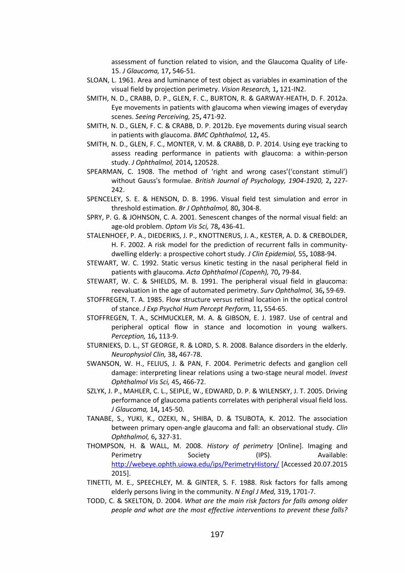
197
assessment of function related to vision, and the Glaucoma Quality of Life-15. J Glaucoma, 17, 546-51.
SLOAN, L. 1961. Area and luminance of test object as variables in examination of the visual field by projection perimetry. Vision Research, 1, 121-IN2.
SMITH, N. D., CRABB, D. P., GLEN, F. C., BURTON, R. & GARWAY-HEATH, D. F. 2012a. Eye movements in patients with glaucoma when viewing images of everyday scenes. Seeing Perceiving, 25, 471-92.
SMITH, N. D., GLEN, F. C. & CRABB, D. P. 2012b. Eye movements during visual search in patients with glaucoma. BMC Ophthalmol, 12, 45.
SMITH, N. D., GLEN, F. C., MONTER, V. M. & CRABB, D. P. 2014. Using eye tracking to assess reading performance in patients with glaucoma: a within-person study. J Ophthalmol, 2014, 120528.
SPEARMAN, C. 1908. The method of ‘right and wrong cases’(‘constant stimuli’) without Gauss's formulae. British Journal of Psychology, 1904-1920, 2, 227-242.
SPENCELEY, S. E. & HENSON, D. B. 1996. Visual field test simulation and error in threshold estimation. Br J Ophthalmol, 80, 304-8.
SPRY, P. G. & JOHNSON, C. A. 2001. Senescent changes of the normal visual field: an age-old problem. Optom Vis Sci, 78, 436-41.
STALENHOEF, P. A., DIEDERIKS, J. P., KNOTTNERUS, J. A., KESTER, A. D. & CREBOLDER, H. F. 2002. A risk model for the prediction of recurrent falls in community-dwelling elderly: a prospective cohort study. J Clin Epidemiol, 55, 1088-94.
STEWART, W. C. 1992. Static versus kinetic testing in the nasal peripheral field in patients with glaucoma. Acta Ophthalmol (Copenh), 70, 79-84.
STEWART, W. C. & SHIELDS, M. B. 1991. The peripheral visual field in glaucoma: reevaluation in the age of automated perimetry. Surv Ophthalmol, 36, 59-69.
STOFFREGEN, T. A. 1985. Flow structure versus retinal location in the optical control of stance. J Exp Psychol Hum Percept Perform, 11, 554-65.
STOFFREGEN, T. A., SCHMUCKLER, M. A. & GIBSON, E. J. 1987. Use of central and peripheral optical flow in stance and locomotion in young walkers. Perception, 16, 113-9.
STURNIEKS, D. L., ST GEORGE, R. & LORD, S. R. 2008. Balance disorders in the elderly. Neurophysiol Clin, 38, 467-78.
SWANSON, W. H., FELIUS, J. & PAN, F. 2004. Perimetric defects and ganglion cell damage: interpreting linear relations using a two-stage neural model. Invest Ophthalmol Vis Sci, 45, 466-72.
SZLYK, J. P., MAHLER, C. L., SEIPLE, W., EDWARD, D. P. & WILENSKY, J. T. 2005. Driving performance of glaucoma patients correlates with peripheral visual field loss. J Glaucoma, 14, 145-50.
TANABE, S., YUKI, K., OZEKI, N., SHIBA, D. & TSUBOTA, K. 2012. The association between primary open-angle glaucoma and fall: an observational study. Clin Ophthalmol, 6, 327-31.
THOMPSON, H. & WALL, M. 2008. History of perimetry [Online]. Imaging and Perimetry Society (IPS). Available: http://webeye.ophth.uiowa.edu/ips/PerimetryHistory/ [Accessed 20.07.2015 2015].
TINETTI, M. E., SPEECHLEY, M. & GINTER, S. F. 1988. Risk factors for falls among elderly persons living in the community. N Engl J Med, 319, 1701-7.
TODD, C. & SKELTON, D. 2004. What are the main risk factors for falls among older people and what are the most effective interventions to prevent these falls?

198
[Online]. Copenhagen, WHO Regional Office for Europe. Health Evidence Network report. Available: http://www.euro.who.int/document/E82552.pdf [Accessed 1 March 2014].
TONAGEL, F., VOYKOV, B. & SCHIEFER, U. 2012. [Conventional perimetry. Antiquated or indispensable for functional glaucoma diagnostics?]. Ophthalmologe, 109, 325-36.
TREUTWEIN, B. 1995. Adaptive psychophysical procedures. Vision Res, 35, 2503-22. TURANO, K. A., RUBIN, G. S. & QUIGLEY, H. A. 1999. Mobility performance in
glaucoma. Invest Ophthalmol Vis Sci, 40, 2803-9. TURPIN, A., ARTES, P. H. & MCKENDRICK, A. M. 2012. The Open Perimetry Interface:
an enabling tool for clinical visual psychophysics. J Vis, 12. TURPIN, A., JANKOVIC, D. & MCKENDRICK, A. M. 2007. Retesting visual fields: utilizing
prior information to decrease test-retest variability in glaucoma. Invest Ophthalmol Vis Sci, 48, 1627-34.
TURPIN, A., MCKENDRICK, A. M., JOHNSON, C. A. & VINGRYS, A. J. 2003. Properties of perimetric threshold estimates from full threshold, ZEST, and SITA-like strategies, as determined by computer simulation. Invest Ophthalmol Vis Sci, 44, 4787-95.
URBAN, F. M. 1910. The method of constant stimuli and its generalizations. Psychological Review, 17, 229.
VAN LANDINGHAM, S. W., MASSOF, R. W., CHAN, E., FRIEDMAN, D. S. & RAMULU, P. Y. 2014. Fear of falling in age-related macular degeneration. BMC Ophthalmol, 14, 10.
VISLISEL, J. M., DOYLE, C. K., JOHNSON, C. A. & WALL, M. 2011. Variability of rarebit and standard perimetry sizes I and III in normals. Optom Vis Sci, 88, 635-9.
VISWANATHAN, A. C., MCNAUGHT, A. I., POINOOSAWMY, D., FONTANA, L., CRABB, D. P., FITZKE, F. W. & HITCHINGS, R. A. 1999. Severity and Stability of Glaucoma: Patient Perception Compared With Objective Measurement. Arch Ophthalmol, 117, 450-454.
VOLBRECHT, V. J., SHRAGO, E. E., SCHEFRIN, B. E. & WERNER, J. S. 2000. Spatial summation in human cone mechanisms from 0 degrees to 20 degrees in the superior retina. J Opt Soc Am A Opt Image Sci Vis, 17, 641-50.
VONTHEIN, R., RAUSCHER, S., PAETZOLD, J., NOWOMIEJSKA, K., KRAPP, E., HERMANN, A., SADOWSKI, B., CHAUMETTE, C., WILD, J. M. & SCHIEFER, U. 2007. The normal age-corrected and reaction time-corrected isopter derived by semi-automated kinetic perimetry. Ophthalmology, 114, 1065-72.
WAKAYAMA, A., MATSUMOTO, C., OHMURE, K., INASE, M. & SHIMOMURA, Y. 2011. Influence of target size and eccentricity on binocular summation of reaction time in kinetic perimetry. Vision Res, 51, 174-8.
WALD, G. 1938. Area and visual threshold. The Journal of general physiology, 21, 269-287.
WALL, M., BRITO, C. F., WOODWARD, K. R., DOYLE, C. K., KARDON, R. H. & JOHNSON, C. A. 2008. Total deviation probability plots for stimulus size v perimetry: a comparison with size III stimuli. Arch Ophthalmol, 126, 473-9.
WALL, M., DOYLE, C. K., ZAMBA, K. D., ARTES, P. & JOHNSON, C. A. 2013. The repeatability of mean defect with size III and size V standard automated perimetry. Invest Ophthalmol Vis Sci, 54, 1345-51.
WALL, M., KUTZKO, K. E. & CHAUHAN, B. C. 1997. Variability in patients with glaucomatous visual field damage is reduced using size V stimuli. Invest Ophthalmol Vis Sci, 38, 426-35.

199
WALL, M., WOODWARD, K. R., DOYLE, C. K. & ARTES, P. H. 2009. Repeatability of automated perimetry: a comparison between standard automated perimetry with stimulus size III and V, matrix, and motion perimetry. Invest Ophthalmol Vis Sci, 50, 974-9.
WALL, M., WOODWARD, K. R., DOYLE, C. K. & ZAMBA, G. 2010. The effective dynamic ranges of standard automated perimetry sizes III and V and motion and matrix perimetry. Arch Ophthalmol, 128, 570-6.
WEBER, J. & RAU, S. 1992. The properties of perimetric thresholds in normal and glaucomatous eyes. Ger J Ophthalmol, 1, 79-85.
WEINREB, R. N., AUNG, T. & MEDEIROS, F. A. 2014. The pathophysiology and treatment of glaucoma: a review. JAMA, 311, 1901-11.
WICHMANN, F. A. & HILL, N. J. 2001a. The psychometric function: I. Fitting, sampling, and goodness of fit. Perception & psychophysics, 63, 1293-1313.
WICHMANN, F. A. & HILL, N. J. 2001b. The psychometric function: II. Bootstrap-based confidence intervals and sampling. Attention, Perception, & Psychophysics, 63, 1314-1329.
WILLIAMS, T. D. 1995. Goldmann field testing in glaucoma. Optom Vis Sci, 72, 532-4. WILSON, M. E. 1970. Invariant features of spatial summation with changing locus in
the visual field. J Physiol, 207, 611-22. WONG, T. Y., KLEIN, B. E., KLEIN, R., KNUDTSON, M. & LEE, K. E. 2003. Refractive
errors, intraocular pressure, and glaucoma in a white population. Ophthalmology, 110, 211-7.
WORLD-HEALTH-ORGANIZATION 1980. International classification of impairments, disabilities, and handicaps: a manual of classification relating to the consequences of disease, published in accordance with resolution WHA29. 35 of the Twenty-ninth World Health Assembly, May 1976.
YARDLEY, L., BEYER, N., HAUER, K., KEMPEN, G., PIOT-ZIEGLER, C. & TODD, C. 2005. Development and initial validation of the Falls Efficacy Scale-International (FES-I). Age Ageing, 34, 614-9.
YOUNG, W. O., STEWART, W. C., HUNT, H. & CROSSWELL, H. 1990. Static threshold variability in the peripheral visual field in normal subjects. Graefes Arch Clin Exp Ophthalmol, 228, 454-7.
ZAR, J. H. 1999. Biostatistical analysis, Pearson Education India. ZULAUF, M. 1994. Normal visual fields measured with Octopus Program G1. I.
Differential light sensitivity at individual test locations. Graefes Arch Clin Exp Ophthalmol, 232, 509-15.
ZULAUF, M., LEBLANC, R. P. & FLAMMER, J. 1994. Normal visual fields measured with Octopus-Program G1. II. Global visual field indices. Graefes Arch Clin Exp Ophthalmol, 232, 516-22.
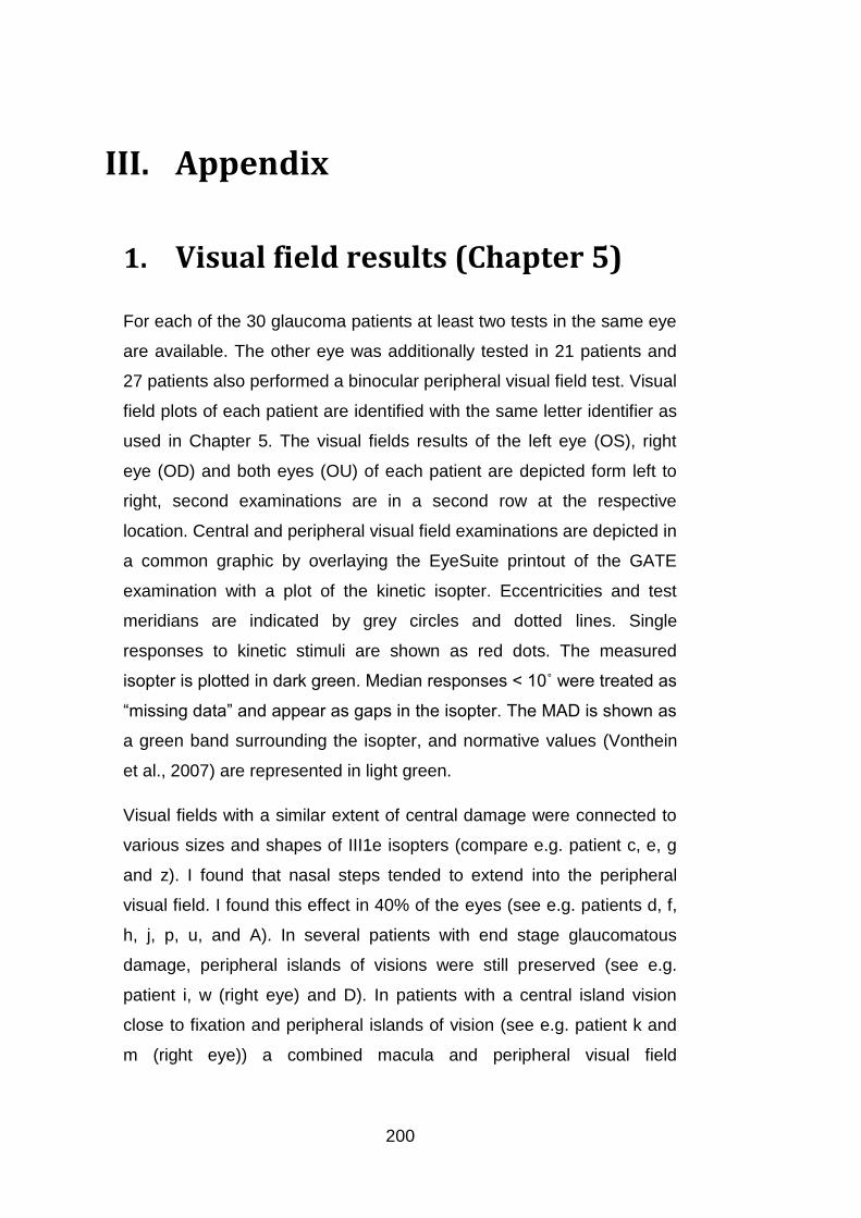
200
III. Appendix
1. Visual field results (Chapter 5)
For each of the 30 glaucoma patients at least two tests in the same eye
are available. The other eye was additionally tested in 21 patients and
27 patients also performed a binocular peripheral visual field test. Visual
field plots of each patient are identified with the same letter identifier as
used in Chapter 5. The visual fields results of the left eye (OS), right
eye (OD) and both eyes (OU) of each patient are depicted form left to
right, second examinations are in a second row at the respective
location. Central and peripheral visual field examinations are depicted in
a common graphic by overlaying the EyeSuite printout of the GATE
examination with a plot of the kinetic isopter. Eccentricities and test
meridians are indicated by grey circles and dotted lines. Single
responses to kinetic stimuli are shown as red dots. The measured
isopter is plotted in dark green. Median responses < 10˚ were treated as
“missing data” and appear as gaps in the isopter. The MAD is shown as
a green band surrounding the isopter, and normative values (Vonthein
et al., 2007) are represented in light green.
Visual fields with a similar extent of central damage were connected to
various sizes and shapes of III1e isopters (compare e.g. patient c, e, g
and z). I found that nasal steps tended to extend into the peripheral
visual field. I found this effect in 40% of the eyes (see e.g. patients d, f,
h, j, p, u, and A). In several patients with end stage glaucomatous
damage, peripheral islands of visions were still preserved (see e.g.
patient i, w (right eye) and D). In patients with a central island vision
close to fixation and peripheral islands of vision (see e.g. patient k and
m (right eye)) a combined macula and peripheral visual field

201
examination might be most suitable. The binocular isopter appeared to
coincide with the respective outer border of the isopters from both eyes,
but stimuli appeared to be detected even slightly further in the periphery
with both than with individual eyes (see e.g. patient a, c, d, m, n and z).

202
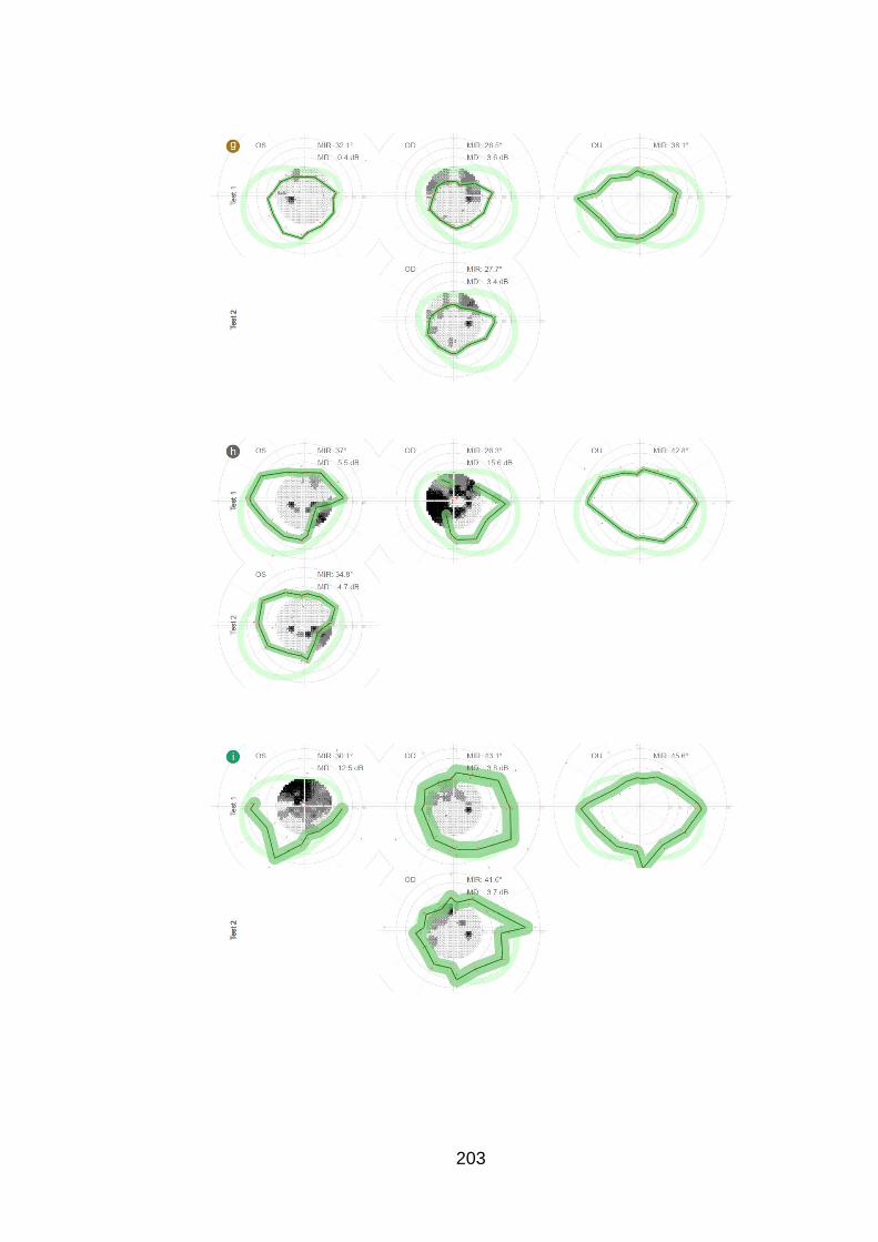
203

204
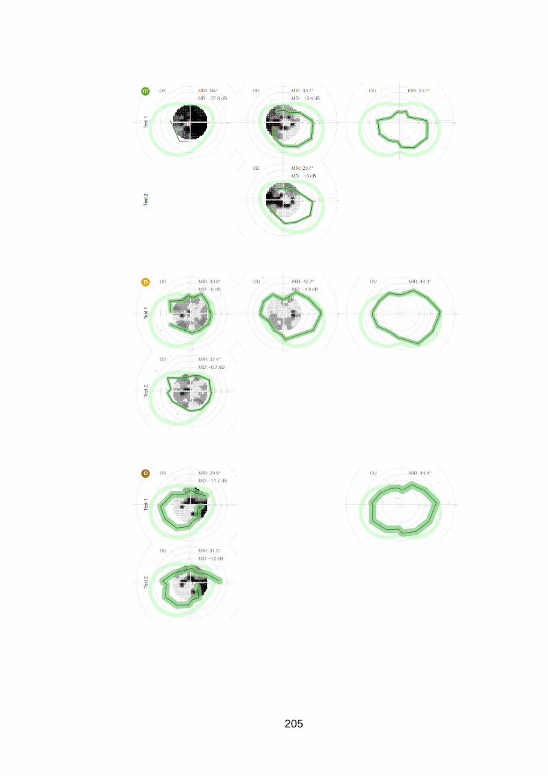
205

206

207
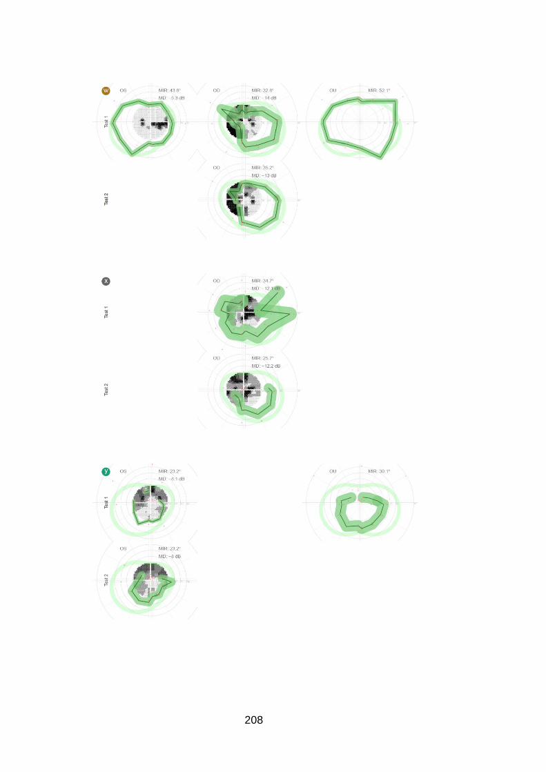
208
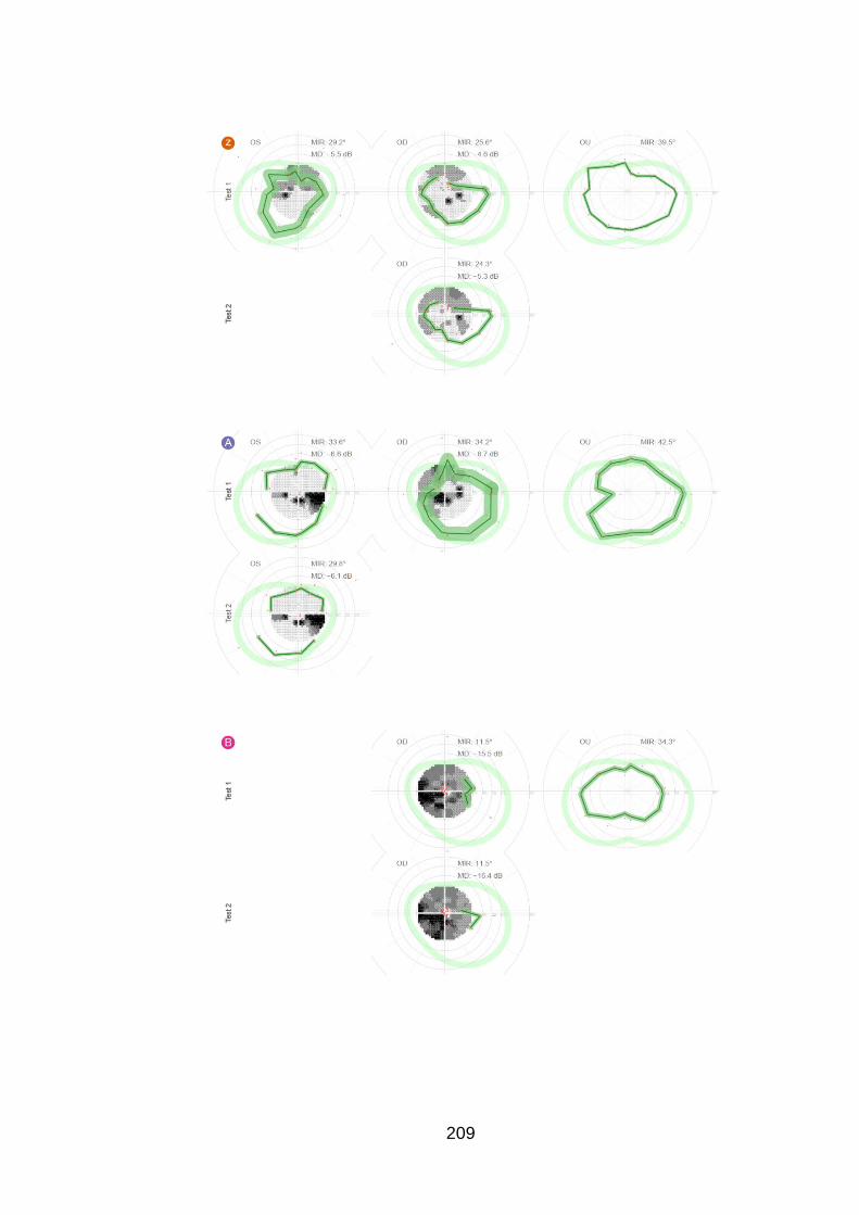
209

210

212
3. How to estimate Bland-Altman
retest intervals in long-tailed
distributions
3.1 Purpose
For clinically useful visual field examinations, it is important that results
are consistent between tests. Thus I investigated the test-retest
variability for a kinetic and static visual field examination (see Chapter
5, page 83). To get a precise estimate of test-retest variability despite
the small sample size, an efficient measure of statistical dispersion
needs to be chosen for the test-retest data. On the other hand, patient
errors occurred that, with a kinetic automatic strategy, are prone to
cause extreme data points, leading to a distribution of test-retest
differences that has long tails. In the kinetic automated procedure three
repeated presentations along each meridian are performed, and the
median is eventually chosen as the isopter position. However, obvious
“outlier” responses occurred in almost all tests of all participants. These
are responses that can be outside normal expected locations and are
often widely spaced away from the true isopter position (see Figure 43).

213
Figure 43: Example of kinetic automatic perimetry illustrating response behaviour. The single responses are marked by red circles. “Outlier” responses are highlighted by arrows.
One of the causes for these false positive responses might be the
audible onset of the projection system’s stepper motors, as many
participants reported to find these noises hard to ignore. If several of
these “outlier” responses occur along the same meridian, the estimated
isopter position can differ substantially from the actual position. This in
turn can lead to extreme differences in test and retest results that are
much stronger than normal response variability. Thus, I wish to use a
measure of dispersion that is representative of the main body of the
data and less sensitive to extreme observations (outliers).
One of the standard techniques to investigate test-retest variability is
Bland-Altman analysis (Bland and Altman, 1986). It analyses the
differences between repeated tests in relation to the true value
(estimated by the average between tests). As an indicator of the
dispersion the 95% limits of agreement give the range within which 19
out of 20 test-retest differences would fall. The 95% range in a Bland-
Altman analysis is defined by ±1.96 standard deviations. In a normal
distribution the standard deviation would be the most efficient measure

214
of statistical dispersion. However, this is not necessarily the case in
distributions that differ from normal. Furthermore using the standard
deviation in a distribution with long tails or outliers could lead to an
overestimation of the sample dispersion that is no longer characteristic
for the majority of observations. Neither the test-retest differences of the
MDs from the static field examinations, nor those of the MIRs from the
kinetic field examinations appear to follow a normal distribution (Figure
44).
Figure 44: Q-Q plots of test-retest distribution for central (MD) and peripheral test (MIR) respectively. Data points deviating from the grey line indicate a non-normal distribution.
The objective of this chapter is to explore, which measure of dispersion
– the standard deviation or the median absolute deviation – is more
efficient for the data in question.
Efficiency measures how precise a measure is depending on sample
size. Robustness of efficiency is precision in the presence of outliers
(Ripley, 2004). To achieve a precise estimate of test-retest variability in
our data, we want to use a measure that is robust. The mean for
example is the most efficient measure of central tendency in a normal
distribution. In samples of the same size the standard error of the mean

215
is lower than that of the median (Figure 45). However, this picture
changes quickly in the presence of outliers. In samples that have as few
as one outlier, the median becomes the more efficient measure of
central tendency. An indicator for the robustness of a measure is the
breakdown point. The breakdown point estimates which proportion of
data points in a distribution may approach infinity without causing the
statistical measure to approach infinity (Ripley, 2004). The breakdown
point for the mean is 0% compared to 50% for the median.
The relative efficiency (RE) of a statistical measure is determined by
comparing the variance of one estimate to the variance of a second
estimate . Unless otherwise stated, is typically assumed to be the
optimal estimator (Ripley, 2004).
Equation 7: Relative efficiency of estimates
The asymptotic relative efficiency (ARE) is the relative efficiency as the
sample size approaches infinity. The asymptotic relative efficiency of
the median is 0.64, which means that the mean is as precise as the
median with only 64% of the data points present (Ripley, 2004).

216
Figure 45: Standard error of mean and median and relative efficiency of median depending on sample size in a normal distribution.
Here, we want to compare efficiency and robustness of two measures
of statistical dispersion: the standard deviation (SD) and the median
absolute deviation (MAD). The standard deviation is defined as the
square root of the mean of the squared differences from the mean. The
median absolute deviation is the median of the absolute deviations from
the median. To compare the variance of standard deviation and median
absolute deviation, they need to be consistent. In normal distributions
the MAD can be scaled by a constant factor of 1.483 to correspond to
the same range as the standard deviation (Figure 46). The scaled MAD
will be referred to as MADsc from here on.

217
Figure 46: Example of normal distribution with SD and MAD and scaling factor to scale the MAD to the same range as one standard deviation.
3.2 Methods
Random samples with varying sample size and outlier proportion were
created in R (version 2.15.1, (R-Core-Team, 2012)) to explore the
efficiency of SD and MADsc through a simulation. Each type of sample
was created 10000 times and the standard error of the measures was
calculated. Normal and long-tailed distributions were specified with a
modified version of the rnorm() function:
rnorm.outl <- function (n=100, a.mean=0, a.sd=1, b.mean=0, b.sd=5,perc=10){
samp <- rnorm(n,0,a.sd) # Creates random normal distribution 1 (samp).
if (perc > 0) { # If percentage of outliers is larger than 0,
samp2 <- rnorm(n,0,b.sd) # creates random normal distribution 2(samp2)
outl <- (n*perc)/100 # and calculates nr of outliers for samp
if (outl%%1 >0) outl <- floor(outl) + rbinom(1,n=1,p=outl-floor(outl))
# with a probabilistic aspect for a non-integer outlier nr.
if (outl >0) samp[1:outl] <- sample(samp2,outl)
# Draws outliers in samp2 and replaces points in samp.
}
return(samp) #return sample
}
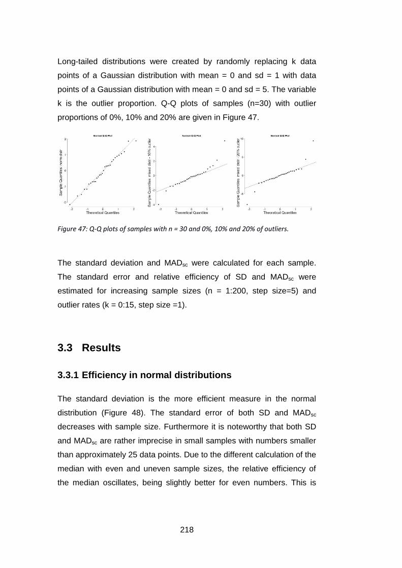
218
Long-tailed distributions were created by randomly replacing k data
points of a Gaussian distribution with mean = 0 and sd = 1 with data
points of a Gaussian distribution with mean = 0 and sd = 5. The variable
k is the outlier proportion. Q-Q plots of samples (n=30) with outlier
proportions of 0%, 10% and 20% are given in Figure 47.
Figure 47: Q-Q plots of samples with n = 30 and 0%, 10% and 20% of outliers.
The standard deviation and MADsc were calculated for each sample.
The standard error and relative efficiency of SD and MADsc were
estimated for increasing sample sizes (n = 1:200, step size=5) and
outlier rates (k = 0:15, step size =1).
3.3 Results
3.3.1 Efficiency in normal distributions
The standard deviation is the more efficient measure in the normal
distribution (Figure 48). The standard error of both SD and MADsc
decreases with sample size. Furthermore it is noteworthy that both SD
and MADsc are rather imprecise in small samples with numbers smaller
than approximately 25 data points. Due to the different calculation of the
median with even and uneven sample sizes, the relative efficiency of
the median oscillates, being slightly better for even numbers. This is

219
especially prominent in small data sets. The asymptotic relative
efficiency of MADsc is 37%.
Figure 48: Standard error of SD and MADsc (upper plot) and relative efficiency of the MADsc in relation to SD (lower plot) with increasing sample size of normally distributed data. The standard deviation is more efficient than the MADsc. In small samples both SD and MAD have large standard errors.
3.3.2 Robustness of efficiency depending on sample size
and outlier proportion
While the standard deviation is the more efficient measure in normally
distributed data, the scaled median absolute deviation is more robust. In
samples with outlier rates larger than 0% the MADsc becomes more
efficient than the SD. The precision of both measures increases with
sample size, however the relative efficiency stays approximately the
same independent of sample size (Figure 49 and Figure 50).

220
Figure 49: Standard error of SD and MADsc depending on outlier rates for sample sizes n = 30 (left) and n = 200 (right). The percentage of outliers ranged from 0 to 20%.
Figure 50: Relative efficiency of SD and MADsc depending on outlier rate for sample sizes of n = 30 (left) and n=90 (right). The percentage of outliers ranged from 0 to 20%.
3.4 Conclusions
While the standard deviation is more efficient in normally distributed
samples, the median absolute deviation is more robust. The MADsc
becomes the more efficient measure of the two as soon as just one
outlier is present in a sample. Since the standard deviation depends on
the mean, which is quite susceptible to extreme values in data sets, it
becomes less precise in data with long tails or outliers and easily
overestimates the statistical dispersion of the data. In contrast, the
median absolute deviation – looking at the differences from the median
– is much more robust. Thus the MAD appears to be the better choice
as a measure of dispersion for our test-retest distributions. One might
argue that the larger test-retest differences in the distributions are not
outliers, but part of the true distribution, thus the MAD would
underestimate dispersion. However, for the clinical relevance of visual

221
field tests, the SD scaled to a 95% range might be too conservative and
might lead to rejecting a test, that still gives valuable information for a
large part of the population.
Based on these findings the MAD was chosen as a measure of
dispersion to fit a 90% range in the Bland-Altman plot for our visual field
test-retest data.
222
4. Power to detect a difference in
dependent correlations
4.1 Purpose
In Chapter 5, I explored the relationship between self reported fear of
falling and summary measures of central and peripheral visual field
results. I found a small but significant relationship between fear of falling
with both central visual field and peripheral visual field test results. The
Spearman correlation coefficients were similar (-0.34 and -0.35
respectively) yet both had large confidence intervals ([-0.65, -0.04] and
[-0.63, -0.05] respectively). For a conclusive study of the relationship
between peripheral and central visual field results and fear of falling
larger samples would be required. Moreover, if one were to study
whether fear of falling is more closely related to one visual field
measure than the other even larger samples are necessary. The two
correlations of peripheral and central measures with fear of falling have
one common variable, here: the fear of falling index. Thus the two
correlations are dependent. This needs to be taken into account when
examining whether the correlations differ. This section is a small
excursion that illustrates this problem through a simulation. I assume
several underlying correlations of samples and evaluate the power of
detecting a significant correlation depending on the number of data
points. I also evaluate the power to detect a significant difference
between two dependent correlations assuming several underlying
correlations. Additionally, I illustrate the effect of noise in samples on
the power to detect a significant difference between dependent
correlations.

223
4.2 Methods
Simulations were programmed in R. To evaluate the power to detect
correlations samples from underlying normal distributions with specified
correlations were drawn with increasing sample sizes from n = 5 to n=
200. For each sample size 500 samples were created. Noise was
introduced by replacing data points of each sample by data points from
random samples with an underlying normal distribution with a standard
deviation of 5 and a mean of 0.
The power to detect a significant correlation or a significant difference
between two correlations was estimated as the percentage of significant
outcomes for each sample size. As a significance test for the difference
between dependent correlations (r12 and r13) Steiger’s z was used. The
equation for Steiger’s z is given below:
; ;
;
;
;
Equation 8: Significance test for dependent correlations: Steiger’s z
4.3 Results
4.3.1 Power to detect a correlation between two samples
Samples with underlying correlation coefficients of 0.25, 0.3, 0.5 and
0.7 were created. The power to detect such correlations depending on
sample size is illustrated in Figure 51. High correlations can be detected
even with relatively small sample sizes while large numbers are needed
to detect small correlations with equivalent power.

224
Figure 51: Power to detect significant correlations with increasing sample size using Spearman correlations. The significance level was chosen as α=0.05, the underlying correlation coefficients of the samples were 0.25, 0.3, 0.5 and 0.75.
4.3.2 Power to detect a difference between two
dependent correlations
Samples 1, 2 and 3 with different underlying dependent correlations (r12
and r13) were created. The correlation coefficients are given in Figure
52. The underlying correlation between sample 2 and 3 (r23) was kept
constant at 0.5. The power to detect a significant correlation depended
on various factors. The power decreased when a lower underlying
difference between the dependent correlations was present or when the
single underlying correlations r12 and r23 were low.
Additionally, the dependent correlations were kept constant and the
underlying correlation between sample 2 and 3 (r23) was varied. The
power to detect a difference between dependent correlations r12 and r13
increased with an increasing underlying correlation r23 (Figure 53).

225
Figure 52: Power of finding a significant difference between two dependent correlation r12 and r13 (with α=0.05) depending on sample size. Samples with various underlying dependent correlation coefficients were created with a constant underlying correlation in r23 of 0.5.
Figure 53: Power of finding a significant difference between two dependent correlation r12 and r13 (with α=0.05) depending on sample size. The samples were chosen to have a 100% increase in the underlying correlations r12 and r13 from 0.25 to 0.5. The underlying correlations in r23 were 0.25, 0.5 and 0.75.

226
4.3.3 Influence of noise in samples on power of detecting
a difference between two dependent correlations
Introducing outliers to the correlated samples expectedly further
decreased the power to detect a significant difference between two
dependent correlations. Figure 54 illustrates adding noise levels of 5%
or 10% has a strong impact on the performance of Spearman
correlations to detect significant correlations.
Figure 54: Influence of noise on detecting the difference between two dependent correlations with increasing sample size. Samples with constant underlying correlations were created and outliers were introduced depicted is the power to detect differences between the dependent correlations in samples without noise and with 5% and 10% outlier rates.
4.4 Conclusions
The results of the simulations demonstrated that the power to detect a
difference between dependent correlations is affected by various
factors. Larger sample sizes are required to have sufficient power when
the difference between the dependent correlations is low or when the
227
single correlation coefficients r12 and r13 are low and even a low
correlation between samples 2 and 3 r23 decreases the power.
Moreover noisy data further reduces the power to detect differences
between dependent correlations. Thus, should there be a difference
between the correlation of central or peripheral visual field summary
measures and fear of falling, large sample sizes would be required to
study such an effect. The correlation coefficients in our small sample
were r12= -0.34 and r13= -0.35 for central and peripheral measures
versus fear of falling respectively. The correlation between central and
peripheral measures was r23 = 0.56. Assuming fear of falling was
actually related more strongly to one visual field measure than the other
with say a difference of 0.2, sample sizes of at least about 250 would be
required for a power of 90%. This is assuming the data has no outliers
and is normally distributed. The sample size of 30 described in Chapter
5 is not sufficient to conclusively study the relation between self
reported fear of falling and central and peripheral visual results.
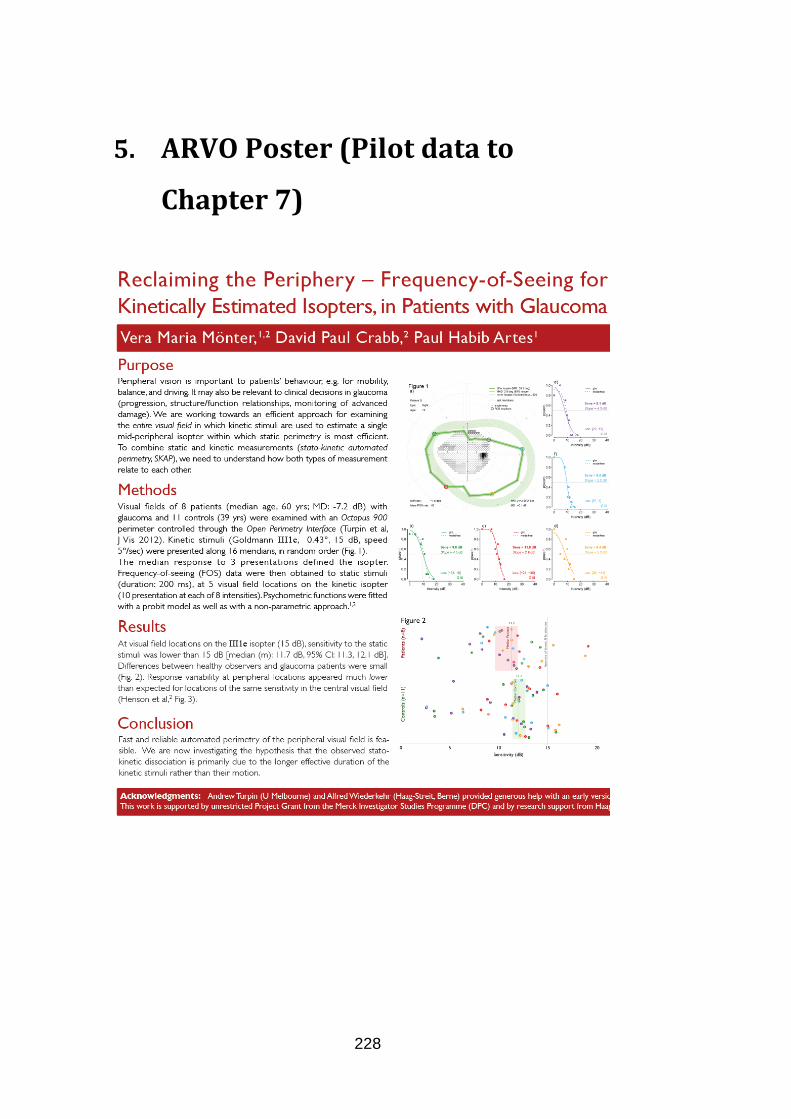
228
5. ARVO Poster (Pilot data to
Chapter 7)

229


![Untitled-5 [cms.esi.info] · Untitled-5 Author: nicole yeardley Created Date: 3/17/2016 3:39:27 PM](https://img.dokumen.tips/doc/110x75/5fd9761b500e945c2c11db24/untitled-5-cmsesiinfo-untitled-5-author-nicole-yeardley-created-date-3172016.jpg)