Embed Size (px)
Citation preview

Computer Science and Software Engineering, 2011
CITS3210 Algorithms
String and File Processing
Notes by CSSE, Comics by xkcd.com
1
Overview
In this topic we will look at pattern-matching
algorithms for strings. Particularly, we will look
at the Rabin-Karp algorithm, the
Knuth-Morris-Pratt algorithm, and the
Boyer-Moore algorithm.
We will also consider a dynamic programming
solution to the Longest Common Substring
problem.
Finally we will examine some file compression
algorithms, including Hu!man coding, and the
Ziv Lempel algorithms.
2
Pattern Matching
We consider the following problem. Suppose T
is a string of length n over a finite alphabet ",
and that P is a string of length m over ".
The pattern-matching problem is to find
occurrences of P within T . Analysis of the
problem varies according to whether we are
searching for all occurrences of P or just the
first occurrence of P .
For example, suppose that we have
" = {a, b, c} and
T = abaaabacccaabbaccaababacaababaac
P = aab
Our aim is to find all the substrings of the text
that are equal to aab.
3
Matches
String-matching clearly has many important
applications — text editing programs being
only the most obvious of these. Other
applications include searching for patterns in
DNA sequences or searching for particular
patterns in bit-mapped images.
We can describe a match by giving the number
of characters s that the pattern must be
shifted along the text in order for every
character in the shifted pattern match the
corresponding text characters. We call this
number a valid shift.
abaaabacccaabbaccaababacaababaac
aab
aab
aab
aab
aab
Here we see that s = 3 is a valid shift.
4

The naive method
The naive pattern matcher simply considers
every possible shift s in turn, using a simple
loop to check if the shift is valid.
When s = 0 we have
abaaabacccaabbaccaababacaababaac
aab
which fails at the second character of the
pattern.
When s = 1 we have
abaaabacccaabbaccaababacaababaac
aab
which fails at the first character of the pattern.
Eventually this will succeed when s = 3.
5
Analysis of the naive method
In the worst case, we might have to examine
each of the m characters of the pattern at
every candidate shift.
The number of possible shifts is n ! m + 1 so
the worst case takes
m(n ! m + 1)
comparisons.
The naive string matcher is ine#cient because
when it checks the shift s it makes no use of
any information that might have been found
earlier (when checking previous shifts).
For example if we have
000000001000001000000010000000
000000001
then it is clear that no shift s " 9 can possibly
work.
6
Rabin-Karp algorithm
The naive algorithm basically consists of two
nested loops — the outermost loop runs
through all the n ! m + 1 possible shifts, and
for each such shift the innermost loop runs
through the m characters seeing if they match.
Rabin and Karp propose a modified algorithm
that tries to replace the innermost loop with a
single comparison as often as possible.
Consider the following example, with alphabet
being decimal digits.
122938491281760821308176283101
176
Suppose now that we have computer words
that can store decimal numbers of size less
than 1000 in one word (and hence compare
such numbers in one operation).
Then we can view the entire pattern as a
single decimal number and the substrings of
the text of length m as single numbers.
7
Rabin-Karp continued
Thus to try the shift s = 0, instead of
comparing
1 ! 7 ! 6
against
1 ! 2 ! 2
character by character, we simply do one
operation comparing 176 against 122.
It takes time O(m) to compute the value 176
from the string of characters in the pattern P .
However it is possible to compute all the
n ! m + 1 decimal values from the text just in
time O(n), because it takes a constant number
of operations to get the “next” value from the
previous.
To go from 122 to 229 only requires dropping
the 1, multiplying by 10 and adding the 9.
8
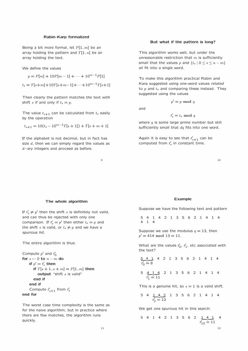
Rabin-Karp formalized
Being a bit more formal, let P [1..m] be an
array holding the pattern and T [1..n] be an
array holding the text.
We define the values
p = P [m] + 10P [m ! 1] + · · · + 10m!1P [1]
ts = T [s+m]+10T [s+m!1]+· · ·+10m!1T [s+1]
Then clearly the pattern matches the text with
shift s if and only if ts = p.
The value ts+1 can be calculated from ts easily
by the operation
ts+1 = 10(ts ! 10m!1T [s + 1]) + T [s + m + 1]
If the alphabet is not decimal, but in fact has
size d, then we can simply regard the values as
d!ary integers and proceed as before.
9
But what if the pattern is long?
This algorithm works well, but under the
unreasonable restriction that m is su#ciently
small that the values p and {ts | 0 " s " n ! m}
all fit into a single word.
To make this algorithm practical Rabin and
Karp suggested using one-word values related
to p and ts and comparing these instead. They
suggested using the values
p# = p mod q
and
t#s = ts mod q
where q is some large prime number but still
su#ciently small that dq fits into one word.
Again it is easy to see that t#s+1 can be
computed from t#s in constant time.
10
The whole algorithm
If t#s $= p# then the shift s is definitely not valid,
and can thus be rejected with only one
comparison. If t#s = p# then either ts = p and
the shift s is valid, or ts $= p and we have a
spurious hit.
The entire algorithm is thus:
Compute p# and t#0for s % 0 to n ! m do
if p# = t#s then
if T [s + 1..s + m] = P [1..m] then
output “shift s is valid”
end if
end if
Compute t#s+1 from t#send for
The worst case time complexity is the same as
for the naive algorithm, but in practice where
there are few matches, the algorithm runs
quickly.
11
Example
Suppose we have the following text and pattern
5 4 1 4 2 1 3 5 6 2 1 4 1 44 1 4
Suppose we use the modulus q = 13, then
p# = 414 mod 13 = 11.
What are the values t#0, t#1, etc associated with
the text?
5 4 1! "# $ 4 2 1 3 5 6 2 1 4 1 4t#0 = 8
5 4 1 4! "# $ 2 1 3 5 6 2 1 4 1 4t#1 = 11
This is a genuine hit, so s = 1 is a valid shift.
5 4 1 4 2! "# $ 1 3 5 6 2 1 4 1 4t#2 = 12
We get one spurious hit in this search:
5 4 1 4 2 1 3 5 6 2 1 4 1! "# $ 4t#10 = 11
12
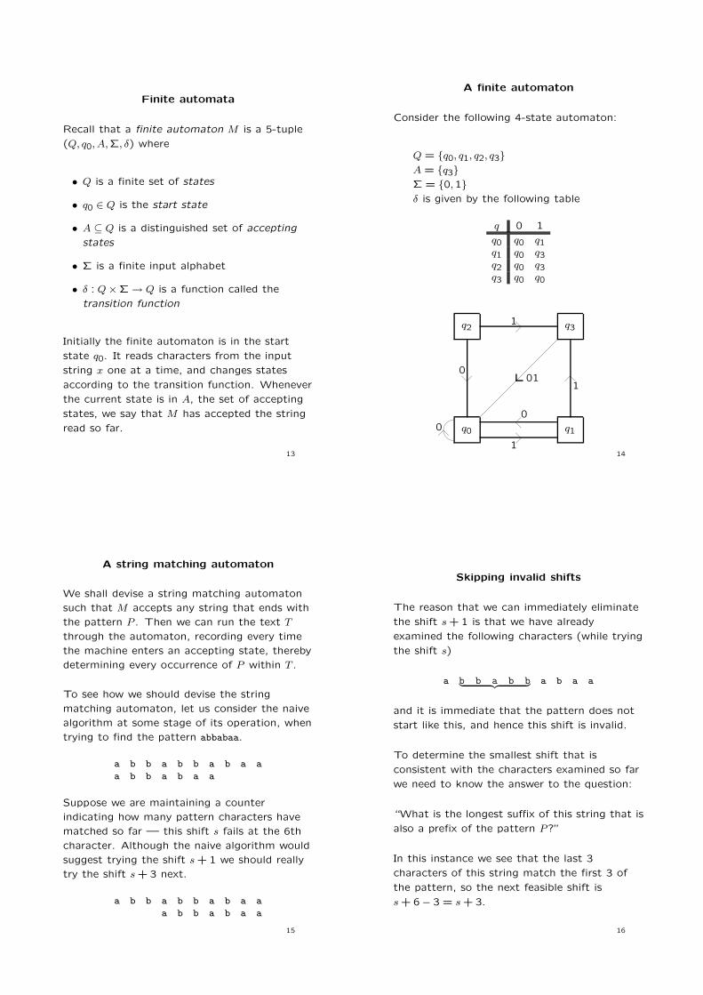
Finite automata
Recall that a finite automaton M is a 5-tuple
(Q, q0, A,", !) where
• Q is a finite set of states
• q0 & Q is the start state
• A ' Q is a distinguished set of accepting
states
• " is a finite input alphabet
• ! : Q ( " ) Q is a function called the
transition function
Initially the finite automaton is in the start
state q0. It reads characters from the input
string x one at a time, and changes states
according to the transition function. Whenever
the current state is in A, the set of accepting
states, we say that M has accepted the string
read so far.
13
A finite automaton
Consider the following 4-state automaton:
Q = {q0, q1, q2, q3}
A = {q3}
" = {0,1}
! is given by the following table
q 0 1
q0 q0 q1q1 q0 q3q2 q0 q3q3 q0 q0
q0 q1
q2 q3
!!
!!
!!
!!
!!
!!
!!
!
"! "!
!"
"!
"!
0
1
1
0
101
!""!
0
14
A string matching automaton
We shall devise a string matching automaton
such that M accepts any string that ends with
the pattern P . Then we can run the text T
through the automaton, recording every time
the machine enters an accepting state, thereby
determining every occurrence of P within T .
To see how we should devise the string
matching automaton, let us consider the naive
algorithm at some stage of its operation, when
trying to find the pattern abbabaa.
a b b a b b a b a aa b b a b a a
Suppose we are maintaining a counter
indicating how many pattern characters have
matched so far — this shift s fails at the 6th
character. Although the naive algorithm would
suggest trying the shift s + 1 we should really
try the shift s + 3 next.
a b b a b b a b a aa b b a b a a
15
Skipping invalid shifts
The reason that we can immediately eliminate
the shift s + 1 is that we have already
examined the following characters (while trying
the shift s)
a b b a b b! "# $ a b a a
and it is immediate that the pattern does not
start like this, and hence this shift is invalid.
To determine the smallest shift that is
consistent with the characters examined so far
we need to know the answer to the question:
“What is the longest su#x of this string that is
also a prefix of the pattern P?”
In this instance we see that the last 3
characters of this string match the first 3 of
the pattern, so the next feasible shift is
s + 6 ! 3 = s + 3.
16

The states
For a pattern P of length m we devise a string
matching automaton as follows:
The states will be
Q = {0,1, . . . , m}
where the state i corresponds to Pi, the
leading substring of P of length i.
The start state q0 = 0 and the only accepting
state is m.
0 1 2 3 4 5 6 7a b b a b a a
"!
"!
"!
"!
"!
"!
"!
This is only a partially specified automaton,
but it is clear that it will accept the pattern P .
We will specify the remainder of the
automaton so that it is in state i if the last i
characters read match the first i characters of
the pattern.
17
The transition function
Now suppose, for example, that the automaton
is given the string
a b b a b b · · ·
The first five characters match the pattern, so
the automaton moves from state 0, to 1, to 2,
to 3, to 4 and then 5. After receiving the sixth
character b which does not match the pattern,
what state should the automaton enter?
As we observed earlier, the longest su#x of this
string that is a prefix of the pattern abbabaa
has length 3, so we should move to state 3,
indicating that only the last 3 characters read
match the beginning of the pattern.
18
The entire automaton
We can express this more formally:
If the machine is in state q and receives a
character c, then the next state should be q#
where q# is the largest number such that Pq# is
a su#x of Pqc.
Applying this rule we get the following finite
state automaton to match the string abbabaa.
0 1 2 3 4 5 6 7a b b a b a a
! #! #
! #
$% $%" &
" &" &
! #
bbaab
a b
b
a
By convention here all the horizontal edges are
pointing to the right, while all the curved line
segments are pointing to the left.
19
Using the automaton
The automaton has the following transition
function:
q a b
0 1 01 1 22 1 33 4 04 1 55 6 36 7 27 1 2
Use it on the following string
ababbbabbabaabbabaabaaabababbabaabbabbaa
Character a b a b b b a b b a bOld state 0 1 2 1 2 3 0 1 2 3 4New state 1 2 1 2 3 0 1 2 3 4 5
Compressing this information:
ababbbabbabaabbabaabaaabababbabaabbabbaa
1212301234567234567211121212345672345341
20

Analysis and implementation
Given a pattern P we must first compute the
transition function. Once this is computed the
time taken to find all occurrences of the
pattern in a text of length n is just O(n) —
each character is examined precisely once, and
no “backing-up” in the text is required. This
makes it particularly suitable when the text
must be read in from disk or tape and cannot
be totally stored in an array.
The time taken to compute the transition
function depends on the size of the alphabet,
but can be reduced to O(m|"|), by a clever
implementation.
Therefore the total time taken by the program
is O(n + m|"|)
Recommended reading: CLRS, Chapter 32,
pages 906–922
21
Regular expressions
22
Knuth-Morris-Pratt
The Knuth-Morris-Pratt algorithm is a
variation on the string matching automaton
that works in a very similar fashion, but
eliminates the need to compute the entire
transition function.
In the string matching automaton, for any
state the transition function gives |"| possible
destinations—one for each of the |"| possible
characters that may be read next.
The KMP algorithm replaces this by just two
possible destinations — depending only on
whether the next character matches the
pattern or does not match the pattern.
As we already know that the action for a
matching character is to move from state q to
q + 1, we only need to store the state changes
required for a non-matching character. This
takes just one array of length m, and we shall
see that it can be computed in time O(m).
23
The prefix function
Let us return to our example where we are
matching the pattern abbabaa.
Suppose as before that we are matching this
against some text and that we detect a
mismatch on the sixth character.
a b b a b x y za b b a b a a
In the string-matching automaton we used
information about what the actual value of x
was, and moved to the appropriate state.
In KMP we do exactly the same thing except
that we do not use the information about the
value of x — except that it does not match
the pattern. So in this case we simply consider
how far along the pattern we could be after
reading abbab — in this case if we are not at
position 5 the next best option is that we are
at position 2.
24

The KMP algorithm
The prefix function " then depends entirely on
the pattern and is defined as follows: "(q) is
the largest k < q such that Pk is a su#x of Pq.
The KMP algorithm then proceeds simply:
q % 0
for i from 1 to n do
while q > 0 and T [i] $= P [q + 1]
q % "(q)
end while
if P [q + 1] = T [i] then
q % q + 1
end if
if q = m then
output “shift of i ! m is valid”
q % "(q)
end if
end for
This algorithm has nested loops. Why is it
linear rather than quadratic?
25
Heuristics
Although the KMP algorithm is asymptotically
linear, and hence best possible, there are
certain heuristics which in some commonly
occurring cases allow us to do better.
These heuristics are particularly e!ective when
the alphabet is quite large and the pattern
quite long, because they enable us to avoid
even looking at many text characters.
The two heuristics are called the bad character
heuristic and the good su!x heuristic.
The algorithm that incorporates these two
independent heuristics is called the
Boyer-Moore algorithm.
26
The algorithm without the heuristics
The algorithm before the heuristics are applied
is simply a version of the naive algorithm, in
which each possible shift s = 0, 1, . . . is tried in
turn.
However when testing a given shift, the
characters in the pattern and text are
compared from right to left. If all the
characters match then we have found a valid
shift.
If a mismatch is found, then the shift s is not
valid, and we try the next possible shift by
setting
s % s + 1
and starting the testing loop again.
The two heuristics both operate by providing a
number other than 1 by which the current shift
can be incremented without missing any
matches.
27
Bad characters
Consider the following situation:
o n c e _ w e _ n o t i c e d _ t h a t
i m b a l a n c e
The two last characters ce match the text but
the i in the text is a bad character.
Now as soon as we detect the bad character i
we know immediately that the next shift must
be at least 6 places or the i will simply not
match.
Notice that advancing the shift by 6 places
means that 6 text characters are not examined
at all.
28

The bad character heuristic
The bad-character heuristic involves
precomputing a function
# : " ) {0,1, . . . , m}
such that for a character c, #(c) is the
right-most position in P where c occurs (and 0
if c does not occur in P).
Then if a mismatch is detected when scanning
position j of the pattern (remember we are
going from right-to-left so j goes from m to
1), the bad character heuristic proposes
advancing the shift by the equation:
s % s + (j ! #(T [s + j]))
Notice that the bad-character heuristic might
occasionally propose altering the shift to the
left, so it cannot be used alone.
29
Good su!xes
Consider the following situation:
t h e _ l a t e _ e d i t i o n _ o f
e d i t e d
The characters of the text that do match with
the pattern are called the good su!x. In this
case the good su!x is ed. Any shift of the
pattern cannot be valid unless it matches at
least the good su#x that we have already
found. In this case we must move the pattern
at least 4 spaces in order that the ed at the
beginning of the pattern matches the good
su#x.
30
The good-su!x heuristic
The good-su#x heuristic involves
precomputing a function
$ : {1, . . . , m} ) {1, . . . , m}
where $(j) is the smallest positive shift of P so
that it matches with all the characters in
P [j + 1..m] that it still overlaps.
We notice that this condition can always be
vacuously satisfied by taking $(j) to be m, and
hence $(j) > 0.
Therefore if a mismatch is detected at
character j in the pattern, the good-su#x
heuristic proposes advancing the shift by
s % s + $(j)
31
The Boyer-Moore algorithm
The Boyer-Moore algorithm simply involves
taking the larger of the two advances in the
shift proposed by the two heuristics.
Therefore, if a mismatch is detected at
character j of the pattern when examining shift
s, we advance the shift according to:
s % s + max($(j), j ! #(T [s + j]))
The time taken to precompute the two
functions $ and # can be shown to be O(m)
and O(|"| + m) respectively.
Like the naive algorithm the worst case is when
the pattern matches every time, and in this
case it will take just as much time as the naive
algorithm. However this is rarely the case and
in practice the Boyer-Moore algorithm
performs well.
32

Example
Consider the pattern:
o n e _ s h o n e _ t h e _ o n e _ p h o n e
What is the last occurrence function #?
c #(c) c #(c) c #(c) c #(c)a 0 h 20 o 21 v 0b 0 i 0 p 19 w 0c 0 j 0 q 0 x 0d 0 k 0 r 0 y 0e 23 l 0 s 5 z 0f 0 m 0 t 11 - 0g 0 n 22 u 0 18
33
Example continued
What is $(22)? This is the smallest shift of P
that will match the 1 character P [23], and this
is 6.
o n e _ s h o n e _ t h e _ o n e _ p h o n e
o n e _ s h o n e _ t h e _ o n e
The smallest shift that matches P [22..23] is
also 6.
o n e _ s h o n e _ t h e _ o n e _ p h o n e
o n e _ s h o n e _ t h e _ o n e
so $(21) = 6.
The smallest shift that matches P [21..23] is
also 6
o n e _ s h o n e _ t h e _ o n e _ p h o n e
o n e _ s h o n e _ t h e _ o n e
so $(20) = 6.
34
However the smallest shift that matches
P [20..23] is 14
o n e _ s h o n e _ t h e _ o n e _ p h o n e
o n e _ s h o n e
so $(19) = 14.
What about $(18)? What is the smallest shift
that can match the characters p h o n e? A
shift of 20 will match all those that are still
left.
o n e _ s h o n e _ t h e _ o n e _ p h o n e
o n e
This then shows us that $(j) = 20 for all
j " 18, so
$(j) =
%
&'
&(
6 20 " j " 2214 j = 1920 1 " j " 18
35
Longest Common Subsequence
Consider the following problem
LONGEST COMMON
SUBSEQUENCE
Instance: Two sequences X and Y
Question: What is a longest common
subsequence of X and Y
Example
If
X = *A, B, C, B, D, A, B+
and
Y = *B, D, C, A, B, A+
then a longest common subsequence is either
*B, C, B, A+
or
*B, D, A, B+
36

A recursive relationship
As is usual for dynamic programming problems
we start by finding an appropriate recursion,
whereby the problem can be solved by solving
smaller subproblems.
Suppose that
X = *x1, x2, . . . , xm+
Y = *y1, y2, . . . , yn+
and that they have a longest common
subsequence
Z = *z1, z2, . . . , zk+
If xm = yn then zk = xm = yn and Zk!1 is a
LCS of Xm!1 and Yn!1.
Otherwise Z is either a LCS of Xm!1 and Y or
a LCS of X and Yn!1.
(This depends on whether zk $= xm or zk $= yn
respectively — at least one of these two
possibilities must arise.)
37
A recursive solution
This can easily be turned into a recursive
algorithm as follows.
Given the two sequences X and Y we find the
LCS Z as follows:
If xm = yn then find the LCS Z # of Xm!1 and
Yn!1 and set Z = Z #xm.
If xm $= yn then find the LCS Z1 of Xm!1 and
Y , and the LCS Z2 of X and Yn!1, and set Z
to be the longer of these two.
It is easy to see that this algorithm requires the
computation of the LCS of Xi and Yj for all
values of i and j. We will let l(i, j) denote the
length of the longest common subsequence of
Xi and Yj.
Then we have the following relationship on the
lengths
l(i, j) =
%
&'
&(
0 if ij = 0l(i ! 1, j ! 1) + 1 if xi = yjmax(l(i ! 1, j), l(i, j ! 1)) if xi $= yj
38
Memoization
The simplest way to turn a top-down recursive
algorithm into a sort of dynamic programming
routine is memoization. The idea behind this is
that the return values of the function calls are
simply stored in an array as they are computed.
The function is changed so that its first step is
to look up the table and see whether l(i, j) is
already known. If so, then it just returns the
value immediately, otherwise it computes the
value in the normal way.
Alternatively, we can simply accept that we
must at some stage compute all the O(n2)
values l(i, j) and try to schedule these
computations as e#ciently as possible, using a
dynamic programming table.
39
The dynamic programming table
We have the choice of memoizing the above
algorithm or constructing a bottom-up
dynamic programming table.
In this case our table will be an
(m + 1) ( (n + 1) table where the (i, j) entry is
the length of the LCS of Xi and Yj.
Therefore we already know the border entries
of this table, and we want to know the value of
l(m, n) being the length of the LCS of the
original two sequences.
In addition to this however we will retain some
additional information in the table - namely
each entry will contain either a left-pointing
arrow %, a upward-pointing arrow , or a
diagonal arrow -.
These arrows will tell us which of the subcases
was responsible for the entry getting that
value.
40
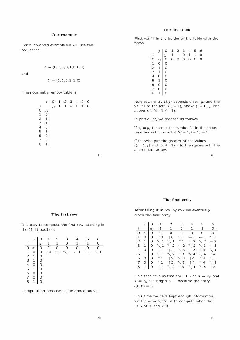
Our example
For our worked example we will use the
sequences
X = *0,1,1,0,1,0,0,1+
and
Y = *1,1,0,1,1,0+
Then our initial empty table is:
j 0 1 2 3 4 5 6i yj 1 1 0 1 1 00 xi1 02 13 14 05 15 07 08 1
41
The first table
First we fill in the border of the table with thezeros.
j 0 1 2 3 4 5 6i yj 1 1 0 1 1 00 xi 0 0 0 0 0 0 01 0 02 1 03 1 04 0 05 1 05 0 07 0 08 1 0
Now each entry (i, j) depends on xi, yj and thevalues to the left (i, j ! 1), above (i ! 1, j), andabove-left (i ! 1, j ! 1).
In particular, we proceed as follows:
If xi = yj then put the symbol - in the square,together with the value l(i ! 1, j ! 1) + 1.
Otherwise put the greater of the valuesl(i ! 1, j) and l(i, j ! 1) into the square with theappropriate arrow.
42
The first row
It is easy to compute the first row, starting in
the (1,1) position:
j 0 1 2 3 4 5 6i yj 1 1 0 1 1 00 xi 0 0 0 0 0 0 01 0 0 , 0 , 0 - 1 % 1 % 1 - 12 1 03 1 04 0 05 1 06 0 07 0 08 1 0
Computation proceeds as described above.
43
The final array
After filling it in row by row we eventually
reach the final array:
j 0 1 2 3 4 5 6i yj 1 1 0 1 1 00 xi 0 0 0 0 0 0 01 0 0 , 0 , 0 - 1 % 1 % 1 - 12 1 0 - 1 - 1 , 1 - 2 - 2 % 23 1 0 - 1 - 2 % 2 - 2 - 3 % 34 0 0 , 1 , 2 - 3 % 3 , 3 - 45 1 0 - 1 - 2 , 3 - 4 - 4 , 46 0 0 , 1 , 2 - 3 , 4 , 4 - 57 0 0 , 1 , 2 - 3 , 4 , 4 - 58 1 0 , 1 - 2 , 3 - 4 - 5 , 5
This then tells us that the LCS of X = X8 and
Y = Y6 has length 5 — because the entry
l(8,6) = 5.
This time we have kept enough information,
via the arrows, for us to compute what the
LCS of X and Y is.
44

Finding the LCS
The LCS can be found (in reverse) by tracingthe path of the arrows from l(m, n). Each
diagonal arrow encountered gives us another
element of the LCS.
As l(8,6) points to l(7,6) so we know that theLCS is the LCS of X7 and Y6.
Now l(7,6) has a diagonal arrow, pointing tol(6,5) so in this case we have found the last
entry of the LCS — namely it is x7 = y6 = 0.
Then l(6,5) points (upwards) to l(5,5), which
points diagonally to l(4,4) and hence 1 is thesecond-last entry of the LCS.
Proceeding in this way, we find that the LCS is
11010
Notice that if at the very final stage of the
algorithm (where we had a free choice) we had
chosen to make l(8,6) point to l(8,5) wewould have found a di!erent LCS
11011
45
Finding the LCS
We can trace back the arrows in our final array,
in the manner just described, to determine that
the LCS is 11010 and see which elements
within the two sequences match.
j 0 1 2 3 4 5 6
i yj 1 1 0 1 1 00 xi 0 0 0 0 0 0 01 0 0 , 0 , 0 - 1 % 1 % 1 - 1
2 1 0 - 1 - 1 , 1 - 2 - 2 % 2
3 1 0 - 1 - 2 % 2 - 2 - 3 % 3
4 0 0 , 1 , 2 - 3 % 3 , 3 - 4
5 1 0 - 1 - 2 , 3 - 4 - 4 , 4
6 0 0 , 1 , 2 - 3 , 4 , 4 - 5
7 0 0 , 1 , 2 - 3 , 4 , 4 - 5
8 1 0 , 1 - 2 , 3 - 4 - 5 , 5
A match occurs whenever we encounter a
diagonal arrow along the reverse path.
See section 15.4 of CLRS for the pseudo-code
for this algorithm.
46
Analysis
The analysis for longest common subsequence
is particularly easy.
After initialization we simply fill in mn entries
in the table — with each entry costing only a
constant number of comparisons. Therefore
the cost to produce the table is $(mn)
Following the trail back to actually find the
LCS takes time at most O(m + n) and
therefore the total time taken is $(mn).
47
Data Compression Algorithms
Data compression algorithms exploit patterns
in data files to compress the files. Every
compression algorithm should have a
corresponding decompression algorithm that
can recover (most of) the original data.
Data compression algorihtms are used by
programs such as WinZip, pkzip and zip. They
are also used in the definition of many data
formats such as pdf, jpeg, mpeg and .doc.
Data compression algorithms can either be
lossless (e.g. for archiving purposes) or lossy
(e.g. for media files).
We will consider some lossless algorithms
below.
48
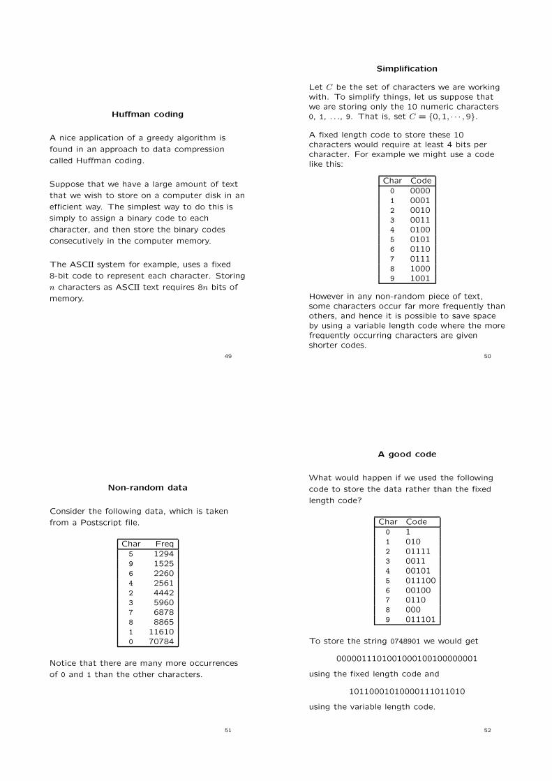
Hu"man coding
A nice application of a greedy algorithm is
found in an approach to data compression
called Hu!man coding.
Suppose that we have a large amount of text
that we wish to store on a computer disk in an
e#cient way. The simplest way to do this is
simply to assign a binary code to each
character, and then store the binary codes
consecutively in the computer memory.
The ASCII system for example, uses a fixed
8-bit code to represent each character. Storing
n characters as ASCII text requires 8n bits of
memory.
49
Simplification
Let C be the set of characters we are workingwith. To simplify things, let us suppose thatwe are storing only the 10 numeric characters0, 1, . . ., 9. That is, set C = {0,1, · · · ,9}.
A fixed length code to store these 10characters would require at least 4 bits percharacter. For example we might use a codelike this:
Char Code0 00001 00012 00103 00114 01005 01016 01107 01118 10009 1001
However in any non-random piece of text,some characters occur far more frequently thanothers, and hence it is possible to save spaceby using a variable length code where the morefrequently occurring characters are givenshorter codes.
50
Non-random data
Consider the following data, which is taken
from a Postscript file.
Char Freq5 12949 15256 22604 25612 44423 59607 68788 88651 116100 70784
Notice that there are many more occurrences
of 0 and 1 than the other characters.
51
A good code
What would happen if we used the following
code to store the data rather than the fixed
length code?
Char Code0 11 0102 011113 00114 001015 0111006 001007 01108 0009 011101
To store the string 0748901 we would get
0000011101001000100100000001
using the fixed length code and
10110001010000111011010
using the variable length code.
52
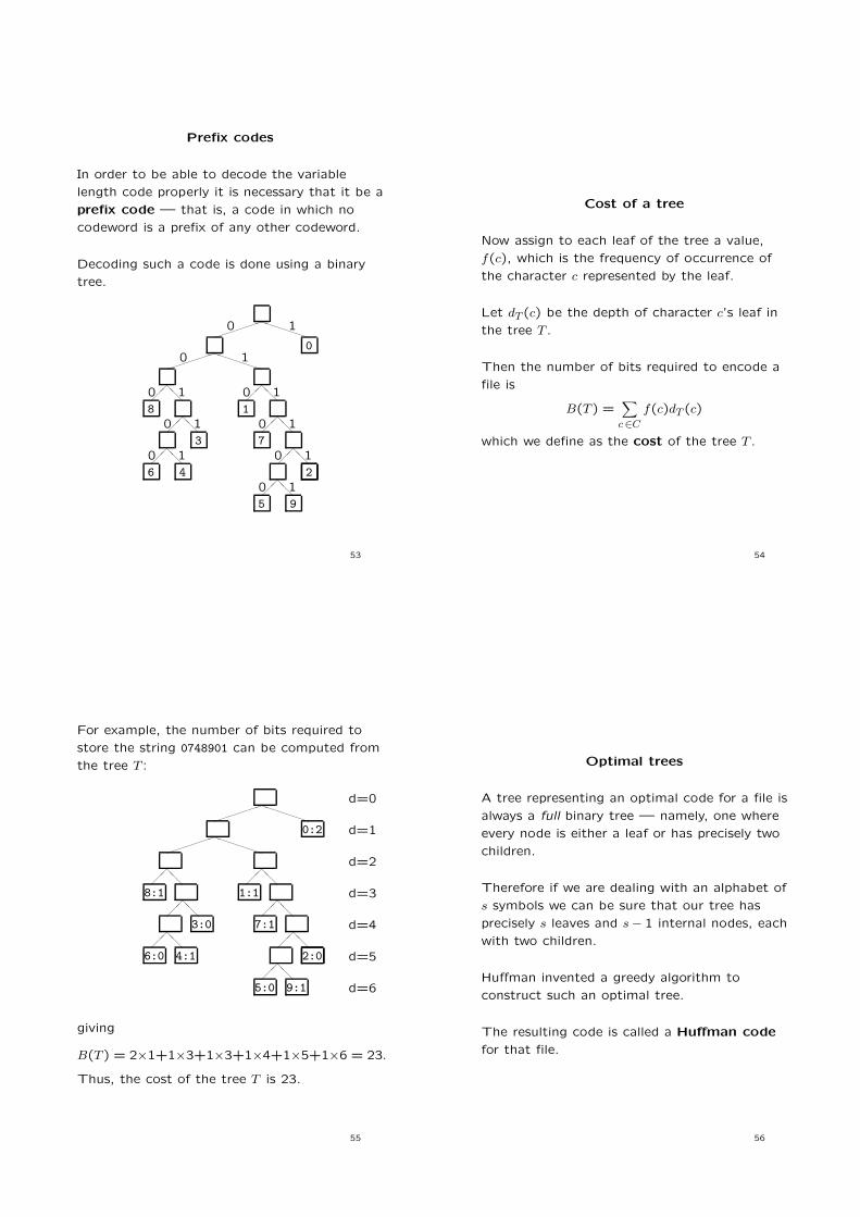
Prefix codes
In order to be able to decode the variable
length code properly it is necessary that it be a
prefix code — that is, a code in which no
codeword is a prefix of any other codeword.
Decoding such a code is done using a binary
tree.
5 9
6 4 2
3 7
8 1
0
!!!
!!!
!!!
!!!
!!!
!!!
!!!
########
########
"""
"""
"""
"""
"""
"""
"""
$$$$$$$$
$$$$$$$$
0
0
0
0 0
0 0
0
0
1
1 1
1 1
1 1
1
1
53
Cost of a tree
Now assign to each leaf of the tree a value,
f(c), which is the frequency of occurrence of
the character c represented by the leaf.
Let dT (c) be the depth of character c’s leaf in
the tree T .
Then the number of bits required to encode a
file is
B(T) =)
c&C
f(c)dT (c)
which we define as the cost of the tree T .
54
For example, the number of bits required to
store the string 0748901 can be computed from
the tree T :
5:0 9:1
6:0 4:1 2:0
3:0 7:1
8:1 1:1
0:2
!!!
!!!
!!!
!!!
!!!
!!!
!!!
########
########
"""
"""
"""
"""
"""
"""
"""
$$$$$$$$
$$$$$$$$
d=6
d=5
d=4
d=3
d=2
d=1
d=0
giving
B(T) = 2(1+1(3+1(3+1(4+1(5+1(6 = 23.
Thus, the cost of the tree T is 23.
55
Optimal trees
A tree representing an optimal code for a file is
always a full binary tree — namely, one where
every node is either a leaf or has precisely two
children.
Therefore if we are dealing with an alphabet of
s symbols we can be sure that our tree has
precisely s leaves and s ! 1 internal nodes, each
with two children.
Hu!man invented a greedy algorithm to
construct such an optimal tree.
The resulting code is called a Hu"man code
for that file.
56

Hu"man’s algorithm
The algorithm starts by creating a forest of s
single nodes, each representing one character,
and each with an associated value, being the
frequency of occurrence of that character.
These values are placed into a priority queue
(implemented as a linear array).
5:1294 9:1525 6:2260 4:2561 2:4442
3:5960 7:6878 8:8865 1:11610 0:70784
Then repeat the following procedure s ! 1
times:
Remove from the priority queue the two nodes
L and R with the lowest values, and create a
internal node of the binary tree whose left child
is L and right child R.
Compute the value of the new node as the
sum of the values of L and R and insert this
into the priority queue.
57
The first few steps
Given the data above, the first two entries o!
the priority queue are 5 and 9 so we create a
new node
5:1294 9:1525
2819!
!"
"
The priority queue is now one element shorter,
as shown below:
6:2260 4:2561 2819
5:1294 9:1525!
!!
"""
2:4442 ...
The next two are 6 and 4 yielding
5:1294 9:1525
2819!
!"
"
6:2260 4:2561
4821 · · ·!
!"
"2:4442
58
Now the smallest two nodes are 2 and the
internal node with value 2819, hence we now
get:
6:2260 4:2561
4821!
!"
"3:5960 7:6878
5:1294 9:1525
2819 2:4442
7261 · · ·!
!"
"
!!
""
Notice how we are growing sections of the tree
from the bottom-up (compare with the tree on
slide 16).
See CLRS (page 388) for the pseudo-code
corresponding to this algorithm.
59
Why does it work?
In order to show that Hu!man’s algorithm
works, we must show that there can be no
prefix codes that are better than the one
produced by Hu!man’s algorithm.
The proof is divided into two steps:
First it is necessary to demonstrate that the
first step (merging the two lowest frequency
characters) cannot cause the tree to be
non-optimal. This is done by showing that any
optimal tree can be reorganised so that these
two characters have the same parent node.
(see CLRS, Lemma 16.2, page 388)
Secondly we note that after making an optimal
first choice, the problem can be reduced to
finding a Hu!man code for a smaller alphabet.
(see CLRS, Lemma 16.3, page 391)
60

Adaptive Hu"man Coding
Hu!man coding requires that we have accurate
estimates of the probablities of each character
occuring.
In general, we can make estimates of the
frequencies of characters occuring in English
text, but these estimates are not useful when
we consider other data formats.
Adaptive Hu!man coding calculates character
frequencies on the fly and uses these dynamic
frequencies to encode characters. This
technique can be applied to binary files as well
as text files.
61
Algorithms: Adaptive Hu"man Coding
The Adaptive Hu"man Coding algorithmsseek to create a Hu!man tree on the fly. AHu!man Coding allows us to encode frequentlyoccurring characters in a lesser number of bitsthan rarely occurring characters. AdaptiveHu!man Coding determines determines theHu!man Tree only from the frequencies of thecharacters already read.
Recall that prefix codes are defined using abinary tree. It can be shown that a prefix codeis optimal if and only if the binary tree has thesibling property.
A binary tree recording the frequency ofcharacters has the sibling property i!
1. every node except the root has a sibling.
2. each right-hand sibling (including non-leafnodes) has at least as high a frequency asits left-hand sibling
(The frequency of non-leaf nodes ins the sumof the frequency of it’s children).
62
Adaptive Hu"man Coding
1 1
1 2 2 2
3 3 4 4
6 6 7 8
12 15
27 33
60
!!!
!!!
!!!
!!!
!!!
!!!
!!!
########
########
"""
"""
"""
"""
"""
"""
"""
$$$$$$$$
$$$$$$$$
0
0
0
0 0
0 0
0
0
1
1 1
1 1
1 1
1
1
63
Adaptive Hu"man Coding
As characters are read it is possible to
e#ciently update the frequencies, and modify
the binary tree so that the sibling property is
preserved. It is also possible to do this in a
deterministic way so that a similar process can
decompress the code.
See
http://www.cs.duke.edu/ jsv/Papers/Vit87.jacmACMversion.pdf
for more details.
As opposed to the LZ algorithms that follow,
Hu!man methods only encode one character
at a time. However, best performance often
comes from combining compression algorithms
(for example, gzip combines LZ77 and
Adaptive Hu"man Coding).
64

Ziv-Lempel compression algorithms
The Ziv-Lempel compression algorithms are a
family of compression algorithms that can be
applied to arbitrary file types.
The Ziv-Lempel algorithms represent recurring
strings with abbreviated codes. There are two
main types:
• LZ77 variants use a bu!er to look for
recurring strings in a small section of the
file.
• LZW variants dynamically create a
dictionary of recurring strings, and assigns
a simple code to each such string.
65
Algorithms: LZ77
The LZ77 algorithms use a sliding window.
The sliding window is a bu!er consisting of the
last m letters encoded (a0...am!1) and the next
n letters to be encoded (b0...bn!1).
Initially we let a0 = a1 = ... = an!1 = w0 and
output *0,0, w+ where w0 is the first letter of
the word to be compressed
The algorithm looks for the longest prefix of
b0...bn!1 appearing in a0...am!1. If the longest
prefix found is b0...bk!1 = ai...ai+k!1, then the
entire prefix is encoded as the tuple
*i, k, bk+
where i is the o"set, k is the length and bk is
the next character.
66
LZ77 Example
Suppose that m = n = 4 and we would like to
compress the word w = aababacbaa
Word Window Outputaababacbaa *0,0, a+
aababacbaa aaaa aaba *0,2, b+
abacbaa aaab a abac *2,3, c+
baa abac baa *1,2, a+
This outputs
*0,0, a+*0, 2, b+*2,3, c+*1,2, a+
67
LZ77 Example cont.
To decompress the code we can reconstruct
the sliding window at each step of the
algorithm. Eg, given
*0,0, a+*0, 2, b+*2,3, c+*1,2, a+
Input Window Output*0,0, a+
*0,2, b+ aaaa aab? aab
*2,3, c+ aaab a abac abac
*1,2, a+ abac baa? baa
Note the trick with the third triple *2,3, c+ that
allows the look-back bu!er to overflow into the
look ahead bu!er. See
http://en.wikipedia.org/wiki/LZ77 and LZ78 for
more information.
68

Algorithms: LZW
The LZW algorithms use a dynamic dictionary
The dictionary maps words to codes and is
initially defined for every byte (0-255). The
compression algorithm is as follows:
w = null
while(k = next byte)
if wk in the dictionary
w = wk
else
add wk to dictionary
output code for w
w = k
output code for w
69
Algorithms: LZW
The decompression algorithm is as follows:
k = next byte
output k
w = k
while(k = next byte)
if there’s no dictionary entry for k
entry = w + first letter of w
else
entry = dictionary entry for k
output entry
add w + first letter of entry to dictionary
w = entry
70
LZW Example
Consider the word w = aababa, and a dictionary
D where D[0] = a, D[1] = b and D[2] = c. The
compression algorithm proceeds as follows:
Read Do Outputa w = a !a w = a, D[3] = aa 0b w = b, D[4] = ab 0a w = a, D[5] = ba 1b w = ab !a w = a, D[6] = aba 4c w = c, D[7] = ac 0b w = b, D[8] = cb 2a w = ba !a w = a, D[9] = baa 5
0
71
LZW Example cont.
To decompress the code *00140250+ we
initialize the dictionary as before. Then
Read Do Output0 w = a a0 w = a, D[3] = aa a1 w = b, D[4] = ab b4 w = ab, D[5] = ba ab0 w = a, D[6] = aba a2 w = c, D[7] = ac c5 w = ba, D[8] = cb ba0 w = a, D[9] = baa a
See
http://en.wikipedia.org/wiki/LZ77 and LZ78,
also.
72

Summary
1. String matching is the problem of finding
all matches for a given pattern, in a given
sample of text.
2. The Rabin-Karp algorithm uses prime
numbers to find matches in linear time in
the expected case.
3. A String matching automata works in linear
time, but requires a significant amount of
precomputing.
4. The Knuth-Morris-Pratt uses the same
principal as a string matching automata,
but reduces the amount of precomputation
required.
73
Summary cont.
5. The Boyer-Moore algorithm uses the bad
character and good su!x heuristics to give
the best performance in the expected case.
6. The longest common subsequence problem
is can be solved using dynamic
programming.
7. Dynammic programming can improve the
e#ciency of divide and conquor algorithms
by storing the resul;ts of sub-computations
so they can be reused later.
8. Data Compression algorithms use pattern
matching to find e#cient ways to compress
file.
74
Summary cont.
9. Hu!man coding uses a greedy approach to
recode the alphabet with a more e#cient
binary code.
10. Adaptive Hu!man coding uses the same
approach, but with the overhead of
precomputing the code.
11. LZ77 uses pattern matching to express
segments of the file in terms of recently
occuring segments.
12. LZW uses a hash function to store
commonly occuring strings so it can refer
to them by their key.
75